Sensitivity Analysis of the Newsboy Model

Avijit Khanra

Chetan Soman

W.P. No. 2013-09-03

September 2013

'

&

$

%

The main objective of the working paper series of the IIMA is to help faculty members,

research stuff, and doctoral students to speedily share their research findings with

professional colleagues and test their research findings at the pre-publication stage. IIMA

is committed to maintain academic freedom. The opinion(s), view(s), and conclusion(s)

expressed in the working paper are those of the authors and not that of IIMA.

Sensitivity analysis of the newsboy model

Avijit Khanra∗1 and Chetan Soman†2

1Doctoral Student, Indian Institute of Management Ahmedabad2Faculty of Production and Quantitative Methods Area, Indian Institute of Management Ahmedabad

Abstract

Sensitivity analysis is an integral part of inventory optimization models due to uncertainty

associated with estimates of model parameters. Though the newsboy problem is one of the

most researched inventory problems, very little is known about its robustness. We study

sensitivity of expected demand-supply mismatch cost to sub-optimal ordering decisions in the

newsboy model. Conditions for symmetry (skewness) of cost deviation have been identified

and magnitude of cost deviation is demonstrated for normal demand distribution. We found

the newsboy model to be sensitive to sub-optimal ordering decisions, much more sensitive

than the economic order quantity model.

1 Introduction

In the newsboy problem, determination of the optimal order quantity (that minimizes expected

demand-supply mismatch cost) requires knowledge of cost parameters and demand distribution

function. All of these may not be known correctly during decision making.

Newsboy deals with stochastic demand, whose realization takes place after the procurement

decision. Hence, theoretically speaking, correct knowledge of the demand distribution (i.e., the

form and associated parameters) with certainty is impossible at the time of decision making.

Unit over-stocking cost is unit purchase cost less unit salvage value (if any). In general,

purchase cost is correctly known at the time of procurement decision. However, if the newsboy

itself is the manufacturer and the production environment is complex (involving multiple items,

etc), purchase cost (i.e., production cost specific to the concerned product) may not be known

correctly. The other component of over-stocking cost, i.e., salvage value, too, may not be known

correctly in many situations. Left-over inventory (if any) is sold at a secondary market (if exists)

and then the remaining stock (if any) is disposed off. This process begins after the selling season

is over and it involves multiple agents, thereby making the assessment of salvage value at the

time of procurement decision difficult.

∗avijitk@iimahd.ernet.in†chetan@iimahd.ernet.in

W.P. No. 2013-09-03 Page No. 2

Unit under-stocking cost is sum of unit profit and unit stock-out goodwill loss. Unit profit

is unit selling price less unit purchase cost. We have already seen that purchase cost may not

be known correctly in some situations. If the selling price is market-driven (e.g., commodity

products), due to time-precedence of the procurement decision over the selling season, actual

selling price may not be known correctly at the time of decision making. The other component

of under-stocking cost, i.e., stock-out goodwill loss is the most elusive cost component in the

newsboy model. Stock-out is reflected back as loss of future demand (of the concerned product

as well as other products) through complex human behaviour, which makes the quantification of

goodwill loss extremely difficult (Prichard & Eagle, 1965).

In absence of correct knowledge of one or more model parameters, estimates are used for

decision making. However, forecasts are rarely correct; the first law of forecasting is that

forecasts are almost always wrong (Bozarth & Handfield, 2006). The procurement decision

using parameter estimates, hence, is rarely optimal (a correct decision using forecasts is a happy

accident). Expected mismatch cost associated with a sub-optimal ordering decision is not the

minimum. Given this unavoidable deviation of operational decision from the optima, it is

important to study the nature of deviation of expected mismatch cost from its minimum (in

short, cost deviation1). Answer to this question, i.e., sensitivity analysis is necessary for better

implementation of the model.

The remainder of the paper is organized as follows. Different elements of sensitivity analysis

are identified in Section 2. Literature review and research objective are discussed in Section 3. In

Section 4, an expression for cost deviation is derived using standard results of the newsboy model.

Necessary and sufficient conditions for symmetry (skewness) of cost deviation are identified

in Section 5. In Section 6, magnitude of cost deviation is demonstrated for normal demand

distribution along with a discussion on “special place” of normal distribution in the family of

symmetric unimodal distributions. A brief study of order quantity deviation along with some

demonstrations is carried out in Section 7. Contributions and their implications are discussed in

Section 8. Finally, we conclude in Section 9.

2 Elements of sensitivity analysis

It is necessary to identify different elements of sensitivity analysis before performing it. Let us

consider a simple optimization problem: minimize y = g(x, p) in x ∈ X, where p represents model

parameter(s). Let us assume that x∗ = h(p) minimizes y. Newsboy model is very similar to this

problem. In fact, many inventory optimization models including the economic order quantity

(EOQ) model are like this. Now, p may not be known correctly; let p be its estimate. Then

the operational decision (probably sub-optimal) is x∗ = h(p). Let δp, δx, δy be the deviations of

p, x, y from their respective true/optimal values. In sensitivity analysis, we study δy.

1Similarly, deviation of order quantity from its optimum is termed as order quantity deviation.

W.P. No. 2013-09-03 Page No. 3

It can be noticed that parameter estimation error influences the objective function via the

decision variable, not “directly”. Sensitivity analysis of this this kind of models have two distinct

parts: i) sensitivity of objective function to sub-optimal decision (δy to δx) and ii) sensitivity of

decision variable to parameter estimation error (δx to δp). Combining these two parts, sensitivity

of objective function to parameter estimation error (δy to δp) can be constructed. In the presence

of multiple parameters, the question of parameter importance (in influencing the objective

function) arises too.

We need to identify what qualifies as component of “sensitivity of δy to δx”. Four components

are listed here: i) direction of deviation, ii) symmetry (skewness) of deviation, iii) magnitude of

deviation, and iv) distribution of deviation. In the literature review, we explore studies on these

four and other relevant components.

Scenario analysis: Before proceeding to the literature review, it is important to distinguish

sensitivity analysis from scenario analysis, a similar post-optimality analysis. In scenario analysis,

we study the nature of change in objective function and decision variable as scenario changes,

i.e., parameter value changes. The issue of sub-optimal decision does not arise here. Let

the new parameter value be p′. Let the deviations from old values be δp′ , δx′ , δy′ . If p = p′,

x∗ = h(p) = h(p′) = x′∗; however, y∗ = g(x∗, p) 6= g(x′∗, p′) = y′∗ as p 6= p′. Then sensitivity

of δx to δp is same as sensitivity of δx′ to δp′ , but other analogous parts differ from each other.

Hence, scenario analysis results regarding the decision variable are valid for sensitivity analysis;

however, the same is not true for the objective function. Scenario analysis studies are included

in literature review for its similarity with sensitivity analysis.

3 Literature review

Sensitivity analysis of some important inventory models are available in literature. EOQ model

is one of the most popular inventory models; one reason for its popularity is its robustness

(less sensitiveness). Sensitivity of cost deviation to sub-optimal order quantity in the EOQ

model can be found in standard textbooks on operations management or inventory management

(e.g., Nahmias, 2001). Cost deviation is left-skewed and relatively insensitive to order quantity

deviation; it grows with the second root of order quantity deviation. Lowe & Schwarz (1983)

and Dobson (1988) studied sensitivity of cost deviation to parameter estimation error in the

EOQ model. They observed insensitivity of cost deviation to parameter estimation error; cost

deviation grows with the fourth root of parameter estimation error. Borgonovo & Peccati (2007)

measured parameter importance in the EOQ model. Inventory holding cost is the most influential

parameter if parameter estimation errors are similar, while the other two parameters (demand

rate and ordering cost) are of equal importance.

Some sensitivity analysis results are available for popular stochastic inventory models. Zheng

(1992) compared stochastic (r,Q) inventory system with its deterministic counterpart (the EOQ

model) and found that the magnitude of cost deviation is less than that of the EOQ model

W.P. No. 2013-09-03 Page No. 4

(which is quite robust itself). F. Chen & Zheng (1997) found similar result for stochastic (s,S)

inventory system with exponential demand. A surprise omission from this list is the newsboy

model, one of the most researched inventory management problems. There are some good

reviews on the newsboy problem (Porteus, 1990; Silver, Pyke, & Peterson, 1998; Khouja, 1999;

Qin, Wang, Vakharia, Chen, & Seref, 2011; Choi, 2012); but, none mention a single focused

study on sensitivity analysis.

Direction of deviation of expected mismatch cost and order quantity can be understood easily

for most cases by having a careful look into the standard results of the newsboy model (available

in good textbooks, e.g., Silver et al., 1998). Since expected mismatch cost is convex in order

quantity, expected mismatch cost always increases whenever order quantity deviates from its

optima (irrespective of the cause for deviation). Order quantity increases with over-estimation

of under-stocking cost and decreases with its under-estimation. This relation is exactly opposite

for over-stocking cost. Order quantity is increasing in mean demand. Impact of demand variance

on order quantity is not so straight forward.

Using mean preserving transformation, Gerchak & Mossman (1992) showed that order

quantity is increasing in demand variability if cf > F (µ); the relation is opposite if cf < F (µ),

where cf, µ, F represent critical factor, mean demand, and demand distribution function. They

also showed that expected mismatch cost is increasing in demand variability (this is a scenario

analysis result regarding the objective function, not valid for sensitivity analysis). Ridder,

van der Laan, & Salomon (1998) provided counter-example to this result; they showed that

expected mismatch cost can be less for more variable demand.

Scenario analysis results (mainly regarding direction of deviation) of some generalized newsboy

problems (i.e., extensions of the standard problem) are available in literature. Lau & Lau (2002)

considered a supply chain with newsboy type retailer and identified impact of demand variability

on decision variables. Their conclusions are similar to that of Gerchak & Mossman (1992) when

order quantity is the only decision variable (i.e., the retailer faces the standard newsboy problem).

Eeckhoudt, Gollier, & Schlesinger (1995) studied risk-averse newsboy problem (risk-neutrality is

equivalent to the standard problem) and identified influence of cost parameters on order quantity;

their findings are similar to what we have already mentioned.

In the newsboy literature, there are studies that develop extensions of the standard newsboy

problem and study sensitivity of expected cost (or expected profit) and order quantity to the

parameter(s) that differentiate it from the standard problem, e.g., L.-H. Chen & Chen (2010)

solved the multi-product budget-constrained newsboy problem with a reservation policy and

studied sensitivity of expected profit and order quantity to budgeted amount. These studies,

being contextually different, do not add much to our understanding of sensitivity of the standard

newsboy model.

Based on the above literature review, the lack of focused studies on sensitivity of the newsboy

model is visible. Our understanding is limited to the knowledge of directions of cost and order

W.P. No. 2013-09-03 Page No. 5

quantity deviations. The questions regarding symmetry, magnitude, and distribution of cost and

order quantity deviations remain largely unanswered. The issue of parameter importance has

not been studied either. In this work, we study symmetry and magnitude of cost deviation as

order quantity deviates from its optimal. We briefly touch the topic of order quantity deviation

to reconfirm the necessity to study cost deviation.

Expected profit maximization objective is equally popular in newsboy set-up. Yet we study

sensitivity of cost deviation because number of parameters is less in the cost minimization

formulation of the newsboy model. Sensitivity of expected profit to sub-optimal order quantity

can be easily obtained from sensitivity of expected cost (see Appendix A).

4 Problem formulation

4.1 Notations and assumptions

a Lower limit of demand. a ≥ 0.

b Upper limit of demand. a < b <∞.

r Ratio of demand limits. r = a/b, r ∈ [0, 1).

F () Distribution function of stochastic demand. F (a) = 0 and F (b) = 1.

f() Density function associated with F . Mere existence of f is assumed; hence, f can

be discontinuous at countable number of points in [a, b]. We also assume existence

of F−1, i.e., f(x) > 0 for almost all x ∈ (a, b).

µ Mean demand.

σ Standard deviation of demand.

cv Coefficient of variation. cv = σ/µ, cv > 0.

cu Unit under-stocking cost. cu > 0.

co Unit over-stocking cost. co > 0.

cf Critical factor. cf = cu/(co + cu), cf ∈ (0, 1).

Q Order quantity. Q ≥ 0. Q∗ denotes its optimal.

C(Q) Demand-supply mismatch cost for a supply of Q.

δQ Deviation of order quantity from its optimal.

δC Deviation of expected mismatch cost from its minimum.

θ Estimate of θ (model parameter). θ can be µ, σ, cu, co, and cf .

δθ Deviation of θ from its true value. θ can be µ, σ, cu, co, and cf .

4.2 The mismatch cost formulation

We follow the mismatch cost formulation of the newsboy model (Silver et al., 1998). Let X be

the random demand. Then mismatch cost is given by

C(Q) = co(Q−X)+ + cu(X −Q)+. (1)

W.P. No. 2013-09-03 Page No. 6

A careful look into the above expression reveals that C(Q < a) > C(Q = a) and C(Q > b) >

C(Q = b) for every possible demand scenario. Thus, the cost minimizing order quantity is in

[a, b]. Expected mismatch cost is given by

E[C(Q)] = co

∫ Q

a(Q− x)f(x)dx+ cu

∫ b

Q(x−Q)f(x)dx

= cu(µ−Q) + (co + cu)

∫ Q

a(Q− x)f(x)dx. (2)

E[C(Q)] may not be differentiable everywhere in (a, b) as f is not necessarily continuous

everywhere in [a, b]. Still, it is fairly easy to establish strict convexity of E[C(Q)] and optimality

of Q∗ = F−1(cf) (see Appendix B). Note that Q∗ is unique as F−1 is strictly increasing.

Minimum expected mismatch cost is given by

E[C(Q∗)] = cuµ− (co + cu)

∫ Q∗

axf(x)dx. (3)

4.3 Expression for cost deviation

We use ratio-based measure for deviation. Ratio-based measure is unit-less; hence, comparison

among deviations is easy. δQ = (Q − Q∗)/Q∗ and δC = (E[C(Q)] − E[C(Q∗)])/E[C(Q∗)].

δQ ≥ −1 as Q ≥ 0 and δC ≥ 0 as E[C(Q)] ≥ E[C(Q∗)]. We derive an expressions for cost

deviation using the demand distribution function. Using (2) and (3),

E[C(Q)]− E[C(Q∗)] = −cuQ+ (co + cu)

[∫ Q

aQf(x)dx−

∫ Q

Q∗xf(x)dx

]= (co + cu)

[Q{F (Q)− cf} −

{QF (Q)−Q∗cf −

∫ Q

Q∗F (x)dx

}]= (co + cu)

∫ Q

Q∗{F (x)− cf}dx.

Similarly, E[C(Q∗)] = (co + cu)

[(µ−Q∗)cf +

∫ Q∗

aF (x)dx

].

Writing Q = Q∗(1 + δQ),

δC(δQ) =

∫ Q∗(1+δQ)Q∗ {F (x)− cf}dx

(µ−Q∗)cf +∫ Q∗a F (x)dx

. (4)

Unlike the EOQ model, where cost deviation is independent of model parameters, δC(δQ)

in the newsboy model depends on cf and F . These dependencies, particularly the presence of

demand distribution function, make the sensitivity analysis complicated. We begin our analysis

with the study of symmetry of δC(δQ) in the next section.

W.P. No. 2013-09-03 Page No. 7

5 Symmetry (skewness) of cost deviation

We identify the conditions for symmetry (skewness) of δC(δQ) w.r.t. δQ = 0. First, we formally

define symmetry, left-skewness, right-skewness, and asymmetry.

Definition 1. Let g be a real-valued function defined on interval I. Let x0 ∈ I and e0 > 0 such

that x0 − e0, x0 + e0 ∈ I. Then we say that g is

i) symmetric in x0 ± e0 if g(x0 − e) = g(x0 + e) ∀e ∈ (0, e0].

ii) left-skewed in x0 ± e0 if g(x0 − e) > g(x0 + e) ∀e ∈ (0, e0].

iii) right-skewed in x0 ± e0 if g(x0 − e) < g(x0 + e) ∀e ∈ (0, e0].

iv) asymmetric in x0 ± e0 if none among the above three holds.

Above definition can be easily modified for functions defined on integer domain.

Following results connect symmetry (skewness) of δC(δQ) in 0± e0 with symmetry (skewness)

of the demand density function, f in Q∗ ± e0Q∗. Since δQ ≥ −1, we restrict e0 ∈ (0, 1] so that

the above definition is valid for δC(δQ).

Proposition 1. δC(δQ) is symmetric in 0± e0 if and only if the demand density function, f is

symmetric almost everywhere in Q∗ ± e0Q∗.

Proof. Denominator of δC(δQ) in (4) is δQ-independent and positive. Then the numerator decides

symmetry (skewness) of δC(δQ). Let D be the denominator. Let ∆(e) = D{δC(0+e)−δC(0−e)}.For every e ∈ (0, e0],

∆(e) =

∫ Q∗(1+e)

Q∗{F (x)− F (Q∗)}dx−

∫ Q∗(1−e)

Q∗{F (x)− F (Q∗)}dx.

Replacing y = |x−Q∗|, i.e., x = Q∗ + y in the first and x = Q∗ − y in the second integral,

∆(e) =

∫ eQ∗

0{F (Q∗ + y)− F (Q∗)} dy −

∫ eQ∗

0{F (Q∗ − y)− F (Q∗)} (−dy)

=

∫ eQ∗

0

[∫ Q∗+y

Q∗f(z)dz −

∫ Q∗

Q∗−yf(z)dz

]dy.

Replacing t = |z −Q∗|, i.e., z = Q∗ + t in the first and z = Q∗ − t in the second inner integral,

∆(e) =

∫ eQ∗

0

[∫ y

0f(Q∗ + t)dt−

∫ 0

yf(Q∗ − t)(−dt)

]dy

=

∫ eQ∗

0

∫ y

0{f(Q∗ + t)− f(Q∗ − t)}dt dy.

W.P. No. 2013-09-03 Page No. 8

Let f be symmetric almost everywhere in Q∗ ± e0Q∗, i.e., f(Q∗ + t) = f(Q∗ − t) for almost

all t ∈ (0, e0Q∗]. Then∫ y

0{f(Q∗ + t)− f(Q∗ − t)}dt = 0 ∀y ∈ (0, e0Q

∗]

⇒∫ eQ∗

0

∫ y

0{f(Q∗ + t)− f(Q∗ − t)}dt dy = 0 ∀e ∈ (0, e0]

⇒ ∆(e) = 0 ≡ δC(e) = δC(−e) ∀e ∈ (0, e0].

Hence, δC(δQ) is symmetric in 0± e0 if f is symmetric almost everywhere in Q∗ ± e0Q∗.

Now, we need to show that if f is not symmetric almost everywhere in Q∗±e0Q∗, δC(δQ) is not

symmetric in 0±e0. If f is not symmetric almost everywhere in Q∗±e0Q∗, f(Q∗+ t) 6= f(Q∗− t)

for uncountable points, t ∈ (0, e0Q∗]. Then

i) ∃ e1 ∈ [0, e0) such that f is symmetric almost everywhere in Q∗ ± e1Q∗.

ii) ∃ e2 ∈ (e1, e0] such that either f(Q∗ + t) > f(Q∗ − t) or f(Q∗ + t) < f(Q∗ − t) for almost

all t ∈ (e1Q∗, e2Q

∗]. This is due to continuity of f almost everywhere in [a, b].

For every e ∈ (e1, e2] ⊆ (0, e0],

∆(e) =

∫ e1Q∗

0

∫ y

0{f(Q∗ + t)− f(Q∗ − t)}dt dy +

∫ eQ∗

e1Q∗

∫ y

0{f(Q∗ + t)− f(Q∗ − t)}dt dy

= 0 +

∫ eQ∗

e1Q∗

[∫ e1Q∗

0{f(Q∗ + t)− f(Q∗ − t)}dt+

∫ y

e1Q∗{f(Q∗ + t)− f(Q∗ − t)}dt

]dy

=

∫ eQ∗

e1Q∗

[0 +

∫ y

e1Q∗{f(Q∗ + t)− f(Q∗ − t)}dt

]dy 6= 0 ⇒ δC(e) 6= δC(−e).

Thus, δC(δQ) is not symmetric in 0±e0 if f is not symmetric almost everywhere in Q∗±e0Q∗.

Density function of uniformly distributed demand is symmetric in Q∗± e0Q∗ for any Q∗ (i.e.,

any cf) if e0 is not large (such that a ≤ Q∗(1 − e0) and Q∗(1 + e0) ≤ b). Then by the above

proposition, δC(δQ) is symmetric. The result related to skewness is somewhat different.

Proposition 2. δC(δQ) is left (right) skewed in 0± e0 if the demand density function, f is left

(right) skewed almost everywhere in Q∗ ± e0Q∗. Conversely, if δC(δQ) is left (right) skewed in

0± e0, f is left (right) skewed almost everywhere in Q∗ ± e′0Q∗ for some e′0 ∈ (0, e0].

Proof. Following the arguments of proposition 1, for every e ∈ (0, e0],

∆(e) =

∫ eQ∗

0

∫ y

0{f(Q∗ + t)− f(Q∗ − t)}dt dy.

W.P. No. 2013-09-03 Page No. 9

Let f be left-skewed almost everywhere in Q∗ ± e0Q∗, i.e., f(Q∗ + t) < f(Q∗ − t) for almost

all t ∈ (0, e0Q∗]. Then∫ y

0{f(Q∗ + t)− f(Q∗ − t)}dt < 0 ∀y ∈ (0, e0Q

∗]

⇒∫ eQ∗

0

∫ y

0{f(Q∗ + t)− f(Q∗ − t)}dt dy < 0 ∀e ∈ (0, e0]

⇒ ∆(e) < 0 ≡ δC(e) < δC(−e) ∀e ∈ (0, e0].

Hence, δC(δQ) is left-skewed in 0± e0 if f is left-skewed almost everywhere in Q∗ ± e0Q∗.

Now we prove the other part of the proposition. By contradiction, let us assume that δC(δQ)

is left-skewed in 0 ± e0, but @ e′0 ∈ (0, e0] such that f is left-skewed almost everywhere in

Q∗ ± e′0Q∗. Then ∃ e′ ∈ (0, e0] such that f(Q∗ + t) ≥ f(Q∗ − t) for almost all t ∈ (0, e′Q∗]. This

is due to continuity of f almost everywhere in [a, b]. Then∫ y

0{f(Q∗ + t)− f(Q∗ − t)}dt ≥ 0 ∀y ∈ (0, e′Q∗]

⇒∫ eQ∗

0

∫ y

0{f(Q∗ + t)− f(Q∗ − t)}dt dy ≥ 0 ∀e ∈ (0, e′]

⇒ ∆(e) ≥ 0 ≡ δC(e) ≥ δC(−e) ∀e ∈ (0, e′].

Hence, δC(δQ) is not left-skewed in 0 ± e′. Since e′ ≤ e0, δC(δQ) is not left-skewed in 0 ± e0,

which is in contradiction with our assumption. Thus, if δC(δQ) is left-skewed in 0 ± e0, f is

left-skewed almost everywhere in Q∗ ± e′0Q∗ for some e′0 ∈ (0, e0].

The proposition can be proved for the case of right-skewness in a very similar manner.

Proposition 1 states that symmetry of the demand density function, f almost everywhere

in Q∗ ± e0Q∗ is both necessary and sufficient for symmetry of cost deviation, δC(δQ) in 0± e0.

These conditions are slightly different for skewness. By proposition 2, left (right) skewness

of f almost everywhere in Q∗ ± e′0Q∗ for some e′0 ∈ (0, e0] is necessary, whereas the same in

Q∗ ± e0Q∗ is sufficient for left (right) skewness of δC(δQ) in 0± e0. Thus, asymmetric demand

density functions may lead to skewness of δC . Only asymmetric demand density functions can

lead to asymmetry of δC . Proposition 1 and 2 have an interesting consequence for symmetric

unimodal demand distributions.

Corollary 1. δC(δQ) is right-skewed if cf < 1/2, left-skewed if cf > 1/2, and symmetric if

cf = 1/2 for symmetric unimodal (in strong sense) demand distributions.

Proof. Here, mean and mode are same. Due to symmetry and strict unimodality, f(x1) < f(x2)

if |µ−x1| > |µ−x2|, f(x1) > f(x2) if |µ−x1| < |µ−x2|, and f(x1) = f(x2) if |µ−x1| = |µ−x2|for any x1, x2 ∈ [a, b]. F (µ) = 1/2 due to symmetry. Let cf, e0 are such that a ≤ Q∗(1− e0) and

Q∗(1 + e0) ≤ b.

W.P. No. 2013-09-03 Page No. 10

If cf < 1/2, Q∗ = F−1(cf) < µ. Then f is right-skewed in Q∗ ± e0 ·Q∗, i.e., f(Q∗ − q) <f(Q∗+q) for every q ∈ (0, e0 ·Q∗] as |µ−(Q∗−q)| = |q+(µ−Q∗)| > |q−(µ−Q∗)| = |µ−(Q∗+q)|.By proposition 2, δC(δQ) is right-skewed in 0± e0.

If cf > 1/2, Q∗ = F−1(cf) > µ. Then f(x) is left-skewed in Q∗ ± e0 ·Q∗, i.e., f(Q∗ − q) >f(Q∗+q) for every q ∈ (0, e0 ·Q∗] as |µ−(Q∗−q)| = |q−(Q∗−µ)| < |q+(Q∗−µ)| = |µ−(Q∗+q)|.By proposition 2, δC(δQ) is left-skewed in 0± e0.

If cf = 1/2, Q∗ = F−1(cf) = µ. Then f(Q∗− q) = f(µ− q) = f(µ+ q) = f(Q∗+ q) for every

q ∈ (0, e0 ·Q∗], i.e., f(x) is symmetric. By proposition 1, δC(δQ) is symmetric in 0± e0.

Many commonly used demand distributions like normal distribution (with proper truncation)

and symmetric triangular distribution are symmetric and unimodal (in strong sense). In these

cases, if cf < 1/2, it is better to under-estimate the order quantity (than over-estimating) and

if cf > 1/2, it is better to over-estimate the order quantity (than under-estimating). Table

1 illustrates this observation. Using (5), δC(δQ) are calculated for different cf for normally

distributed demand with cv = 0.25 (no truncation). It is evident that δC(δQ) is right-skewed for

cf = 0.25, left-skewed for cf = 0.75, and symmetric for cf = 0.5.

Table 1: Symmetry (skewness) of δC(δQ) for normal demand

cfδQ

-5% 5% -10% 10% -15% 15% -20% 20%

0.25 1.33 1.43 5.09 5.91 10.9 13.7 18.6 24.8

0.50 1.99 1.99 7.90 7.90 17.5 17.5 30.4 30.4

0.75 2.87 2.58 11.9 9.70 27.7 20.4 50.3 33.8

6 Normal demand distribution

Let us turn our attention to the study of magnitude of cost deviation. δC(δQ) depends on cf and

F . Since cf ∈ (0, 1), we can capture dependence of δC on cf by considering different scenarios

(different values of cf). On the other hand, F can be “anything”; there is no simple way to

capture dependence of δC on F . In this situation, study of specific demand distribution(s) is a

way-out. When it comes to demand modelling, normal distribution is the natural choice. It is

widely used for demand modelling in the newsboy and inventory management literature (Silver

et al., 1998). Another reason for choosing normal distribution is its “special place” in the family

of symmetric unimodal distributions (discussed next), which allows us to generalize our findings

from the study with normal distribution to the family of symmetric unimodal distributions.

W.P. No. 2013-09-03 Page No. 11

6.1 Symmetric unimodal demand

We assume following three properties to hold for stochastic demand in a newsboy set-up.

I. Boundedness: Demand has finite non-negative lower limit and positive upper limit, i.e., F

has a bounded interval support [a, b], 0 ≤ a < b <∞.

II. Unimodality : Demand distribution is unimodal, i.e., F is convex in [a, c] and concave in

[c, b], where c is the mode (Gkedenko & Kolmogorov, 1954).

III. Symmetry : Demand density is symmetric, i.e. f(a+ x) = f(b− x) ∀x ∈ [0, b− a].

It is impossible to find an exception to the boundedness property in a real life situation.

The unimodality property, too, holds in general; most demand distributions in the literature

are unimodal. The symmetry property is somewhat restrictive; still, many real life newsboy

demand can be adequately modelled by symmetric distributions. Popular distributions for

demand modelling such as uniform, symmetric triangular, and symmetric truncated normal

distributions satisfy above properties. The set of symmetric unimodal demand distributions in

[a, b] is denoted by Da,b.

We do not need to assume existence of F−1 separately for F ∈ Da,b because unimodality

ensures that f(x) > 0 ∀x ∈ (a, b). If f(a′ > a) = 0, F (a′) = 0; then a can not be the lower limit.

Similarly, if f(b′ < b) = 0, F (b′) = 1; then b can not be the upper limit. Here, mean and mode

are same due to symmetry of f . For the same reason, µ = (a+ b)/2 and F (µ) = 1/2 for every

F ∈ Da,b. F ∈ Da,b admits following bounds (see Appendix C for a proof).

Lemma 1. F0(x) < F (x) ≤ FU (x) if x ∈ (a, µ) and FU (x) ≤ F (x) < F0(x) if x ∈ (µ, b) for

every F ∈ Da,b, where F0(x) = 0 if x ∈ [a, µ), F0(x) = 1 if x ∈ [µ, b] and FU is the uniform

distribution in [a, b].

Figure 1 demonstrates the bounds of Da,b. The thick straight line is FU . The remaining

curves correspond to symmetric truncated normal distribution for different values of coefficient

of variation (in short, FN(cv)). cv = 0.01, 0.03, 0.05, 0.07, 0.1, 0.14, 0.2, 0.3 have been considered;

cv = 0.01 is closest to F0 and cv = 0.3 is closest to FU .

Any combination of a convex increasing curve connecting (a, 0), (µ, 0.5) and a concave

increasing curve connecting (µ, 0.5), (b, 1) with the additional property of symmetry is a member

of Da,b. FN(cv) assumes different forms between the bounds of Da,b for different values of cv. In

fact, FN(cv) asymptotically approaches bounds of Da,b.

Lemma 2. FN(cv) → FU as cv → ∞ and FN(cv) → F0 as cv → 0+ except around the mean,

where FU and F0 are bounds of F ∈ Da,b.

A proof of the above lemma appears in Appendix D. Due to versatility of shape of FN(cv),

by studying cost deviation for FN(cv) with different cv values, we can get a fair idea about the

magnitude of cost deviation for the newsboy model (for F ∈ Da,b).

W.P. No. 2013-09-03 Page No. 12

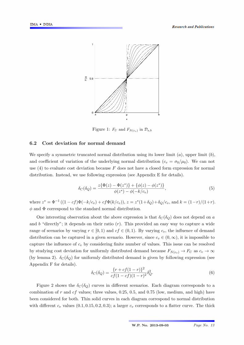
Figure 1: FU and FN(cv) in Da,b

6.2 Cost deviation for normal demand

We specify a symmetric truncated normal distribution using its lower limit (a), upper limit (b),

and coefficient of variation of the underlying normal distribution (cv = σ0/µ0). We can not

use (4) to evaluate cost deviation because F does not have a closed form expression for normal

distribution. Instead, we use following expression (see Appendix E for details).

δC(δQ) =z{Φ(z)− Φ(z∗)}+ {φ(z)− φ(z∗)}

φ(z∗)− φ(−k/cv), (5)

where z∗ = Φ−1 ((1− cf)Φ(−k/cv) + cfΦ(k/cv)), z = z∗(1+δQ)+δQ/cv, and k = (1−r)/(1+r).

φ and Φ correspond to the standard normal distribution.

One interesting observation about the above expression is that δC(δQ) does not depend on a

and b “directly”; it depends on their ratio (r). This provided an easy way to capture a wide

range of scenarios by varying r ∈ [0, 1) and cf ∈ (0, 1). By varying cv, the influence of demand

distribution can be captured in a given scenario. However, since cv ∈ (0,∞), it is impossible to

capture the influence of cv by considering finite number of values. This issue can be resolved

by studying cost deviation for uniformly distributed demand because FN(cv) → FU as cv →∞(by lemma 2). δC(δQ) for uniformly distributed demand is given by following expression (see

Appendix F for details).

δC(δQ) ={r + cf(1− r)}2

cf(1− cf)(1− r)2δ2Q. (6)

Figure 2 shows the δC(δQ) curves in different scenarios. Each diagram corresponds to a

combination of r and cf values; three values, 0.25, 0.5, and 0.75 (low, medium, and high) have

been considered for both. Thin solid curves in each diagram correspond to normal distribution

with different cv values (0.1, 0.15, 0.2, 0.3); a larger cv corresponds to a flatter curve. The thick

W.P. No. 2013-09-03 Page No. 13

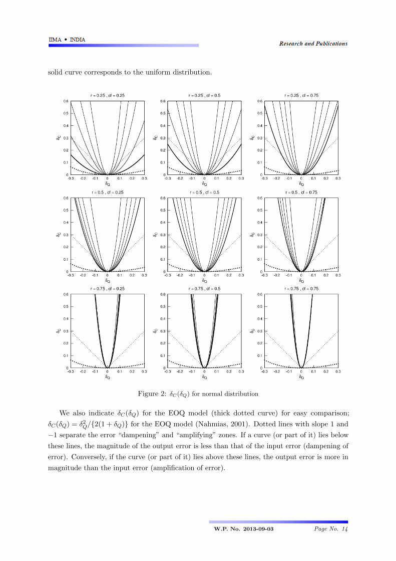
solid curve corresponds to the uniform distribution.

Figure 2: δC(δQ) for normal distribution

We also indicate δC(δQ) for the EOQ model (thick dotted curve) for easy comparison;

δC(δQ) = δ2Q/{2(1 + δQ)} for the EOQ model (Nahmias, 2001). Dotted lines with slope 1 and

−1 separate the error “dampening” and “amplifying” zones. If a curve (or part of it) lies below

these lines, the magnitude of the output error is less than that of the input error (dampening of

error). Conversely, if the curve (or part of it) lies above these lines, the output error is more in

magnitude than the input error (amplification of error).

W.P. No. 2013-09-03 Page No. 14

Key observations

i) FN(cv) and FU curves are steeper than the EOQ curve. Very small part of the FN(cv)

curves lie below the ±1 slope lines.

ii) Steepness of FN(cv) and FU curves decrease in cv and increase in r and cf .

Greater steepness of the FN(cv) and FU curves compared to the EOQ curve convincingly

demonstrates that the newsboy model is more sensitive to sub-optimal order quantities than the

EOQ model. Like EOQ curve, the ±1 slope lines act as benchmark. Locations of the FN(cv)

curves imply that amplification of error occurs in many situations.

From the behaviour of the FN(cv) and FU curves as cv and r change, we can conclude that

robustness of the newsboy model deteriorates with decrease in cv and increase in r. This

behaviour can be explained by flattening of the density function due to increased cv or decreased

r. In both cases, the numerator of cost deviation,∫ QQ∗{F (x) − cf}dx =

∫ QQ∗(Q − x)f(x)dx

decreases, thereby decreasing δC(δQ). The effect reverses when cv decreases or r increases.

When cf is high, Q∗ is high; then Q = Q∗(1 + δQ) is at a greater distance from Q∗ compared

to a low cf case. A higher |Q−Q∗| increases the numerator of cost deviation,∫ QQ∗{F (x)− cf}dx,

thereby increasing δC(δQ). This explains behaviour of the FN(cv) and FU curves as cf changes.

This behaviour is mainly due to the choice of measurement of deviation. We may not observe

the same pattern if deviation is measured by change in value.

The special case of r = 0

In Figure 2, r = 0.25, 0.5, 0.75 have been considered. Theoretically, r ∈ [0, 1). Though very high

value of r is uncommon, very low value, on the other hand, is quite common, e.g., demand limits

of 10 and 100 gives a r value of 0.1.

Figure 3: δC(δQ) for normal distribution when r = 0

Figure 3 demonstrates the special case of r = 0. The construction of the diagrams is very

similar to that of Figure 2. The magnitude of cost deviation decreases, but still remains at

W.P. No. 2013-09-03 Page No. 15

a much higher level than the benchmarks. Our observations with Figure 2 (and associated

conclusions) hold for this special case.

7 Order quantity deviation: Some remarks

Figure 2 demonstrates that the penalty for deviation from the optima in the newsboy model in a

“common” setting (i.e., normal demand distribution and practical values for model parameters)

can be very high. However, the knowledge of cost deviation without any understanding order

quantity deviation is incomplete. In this section, we study order quantity deviation.

Let Z = (X − µ)/σ be the standardized random variable associated with X. E[Z] = 0 and

V ar(Z) = 1. Let Fz be the distribution function associated with Z. Fz(z) = F (µ+ zσ). The

optimum order quantity in newsboy problem can be expressed as Q∗ = µ + σF−1z (cf). The

operational order quantity is given by Q∗ = µ + σF−1z (cf). It is assumed that the form of

demand distribution is correctly known. Using these expressions of Q∗ and Q∗, order quantity

deviation, δQ = (Q∗ −Q∗)/Q∗ can be expressed as

δQ ={µ(1 + δµ)− µ}+ {σ(1 + δσ)F−1

z (cf(1 + δcf ))− σF−1z (cf)}

µ+ σF−1z (cf)

⇒ δQ =δµ + cv{(1 + δσ)F−1

z (cf(1 + δcf ))− F−1z (cf)}

1 + cvF−1z (cf)

. (7)

Above equation can be rewritten as δQ = (δµ + cvδσ×cf )/{1 + cvF−1z (cf)}, where δσ×cf =

(1 + δσ)F−1z (cf(1 + δcf ))− F−1

z (cf) is the joint impact of δσ and δcf on δQ. Impact of δµ and

δσ×cf on δQ is straight forward; δQ increases in both. If cv < 1, impact of δµ is stronger than

that of δσ×cf (assuming magnitudes of δµ and δσ×cf of same level). Thus, mean demand may be

the most influential parameter in the newsboy model if cv is not very high.

δσ and δcf impact δσ×cf in a complex manner; a thorough investigation would require a

dedicated study. Here, we demonstrate the influence of δσ, δcf on δσ×cf and δµ, δσ×cf on δQ with

an example. Before that, it should be noted that δcf is determined by interaction of δcu and δco .

δcf = cf/cf − 1 can be expressed as

δcf =cu(co + cu)

(co + cu)cu− 1 =

cuco − cuco{(1 + δco) + (cu/co)(1 + δcu)}cuco

=(1 + δcu)− (1 + δco)

1 + δco + cf1−cf (1 + δcu)

⇒ δcf =(1− cf)(δcu − δco)

1 + cfδcu + (1− cf)δco. (8)

Two properties can be readily observed about δcf : i) high cf leads to lower magnitude level

of δcf compared to low cf and ii) same signs of δcu and δco leads to lower magnitude level of δcf

compared to opposite signs. Our demonstration confirms these observations.

Table 2 demonstrates δQ in different deviation scenarios for normal demand distribution

W.P. No. 2013-09-03 Page No. 16

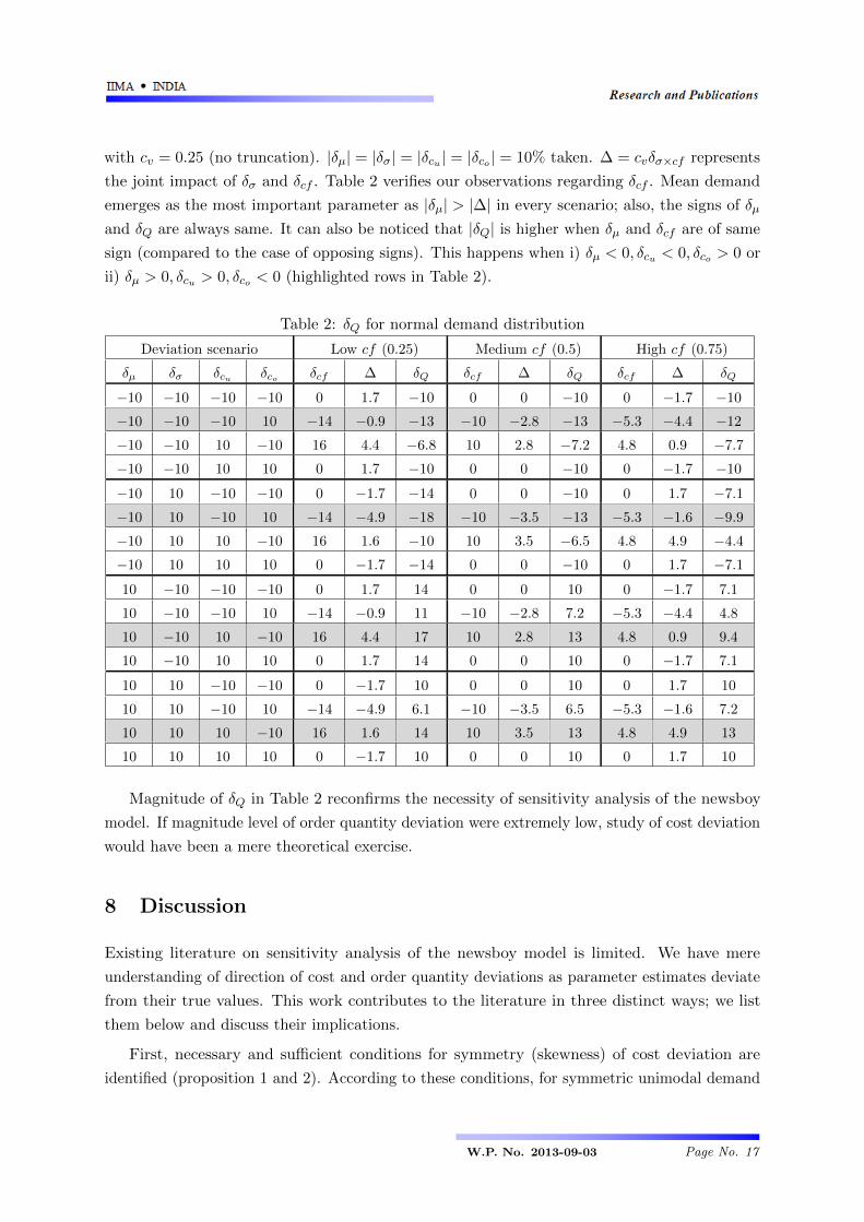
with cv = 0.25 (no truncation). |δµ| = |δσ| = |δcu | = |δco | = 10% taken. ∆ = cvδσ×cf represents

the joint impact of δσ and δcf . Table 2 verifies our observations regarding δcf . Mean demand

emerges as the most important parameter as |δµ| > |∆| in every scenario; also, the signs of δµ

and δQ are always same. It can also be noticed that |δQ| is higher when δµ and δcf are of same

sign (compared to the case of opposing signs). This happens when i) δµ < 0, δcu < 0, δco > 0 or

ii) δµ > 0, δcu > 0, δco < 0 (highlighted rows in Table 2).

Table 2: δQ for normal demand distribution

Deviation scenario Low cf (0.25) Medium cf (0.5) High cf (0.75)

δµ δσ δcu δco δcf ∆ δQ δcf ∆ δQ δcf ∆ δQ

−10 −10 −10 −10 0 1.7 −10 0 0 −10 0 −1.7 −10

−10 −10 −10 10 −14 −0.9 −13 −10 −2.8 −13 −5.3 −4.4 −12

−10 −10 10 −10 16 4.4 −6.8 10 2.8 −7.2 4.8 0.9 −7.7

−10 −10 10 10 0 1.7 −10 0 0 −10 0 −1.7 −10

−10 10 −10 −10 0 −1.7 −14 0 0 −10 0 1.7 −7.1

−10 10 −10 10 −14 −4.9 −18 −10 −3.5 −13 −5.3 −1.6 −9.9

−10 10 10 −10 16 1.6 −10 10 3.5 −6.5 4.8 4.9 −4.4

−10 10 10 10 0 −1.7 −14 0 0 −10 0 1.7 −7.1

10 −10 −10 −10 0 1.7 14 0 0 10 0 −1.7 7.1

10 −10 −10 10 −14 −0.9 11 −10 −2.8 7.2 −5.3 −4.4 4.8

10 −10 10 −10 16 4.4 17 10 2.8 13 4.8 0.9 9.4

10 −10 10 10 0 1.7 14 0 0 10 0 −1.7 7.1

10 10 −10 −10 0 −1.7 10 0 0 10 0 1.7 10

10 10 −10 10 −14 −4.9 6.1 −10 −3.5 6.5 −5.3 −1.6 7.2

10 10 10 −10 16 1.6 14 10 3.5 13 4.8 4.9 13

10 10 10 10 0 −1.7 10 0 0 10 0 1.7 10

Magnitude of δQ in Table 2 reconfirms the necessity of sensitivity analysis of the newsboy

model. If magnitude level of order quantity deviation were extremely low, study of cost deviation

would have been a mere theoretical exercise.

8 Discussion

Existing literature on sensitivity analysis of the newsboy model is limited. We have mere

understanding of direction of cost and order quantity deviations as parameter estimates deviate

from their true values. This work contributes to the literature in three distinct ways; we list

them below and discuss their implications.

First, necessary and sufficient conditions for symmetry (skewness) of cost deviation are

identified (proposition 1 and 2). According to these conditions, for symmetric unimodal demand

W.P. No. 2013-09-03 Page No. 17

distributions (e.g., normal distribution), it is better to under-estimate the order quantity (than

over-estimating) if cf < 1/2 and it is better to over-estimate the order quantity (than under-

estimating) if cf > 1/2 (corollary 1). Based on experiments, Schweitzer & Cachon (2000)

reported that managers order more than the optimal when cf < 1/2 and less than the optimal

when cf > 1/2. They considered symmetric unimodal demand distribution. Kevork (2010)

developed estimators for order quantity and expected profit for normal demand distribution.

He, too, observed that the order quantity is over-estimated when cf < 1/2 and under-estimated

when cf > 1/2. Our finding suggests that expected profit maximizing managers are better off

doing the opposite if one is uncertain about the optimal order quantity.

Second, we demonstrate magnitude level of cost deviation for normal demand distribution

(Figure 2) and compared it with two benchmarks (cost deviation of the EOQ model and ±1

slope lines). The EOQ model is robust, i.e., increase in inventory costs due to sub-optimal

ordering decision is very low. Popular stochastic inventory models like (r,Q) and (s,S) inventory

systems have been found to be more robust than the EOQ model (by Zheng, 1992; F. Chen &

Zheng, 1997). Newsboy model is an exception; it is much more sensitive to sub-optimal ordering

decisions than the EOQ model. In fact, in many situations, magnitude of cost deviation exceeds

the magnitude of the input error. This is a clear signal to the practitioners to take proper care of

the parameter estimation processes so that the order quantity deviation is small. Cost deviation

increases with ratio of demand limits (r) and decreases with coefficient of variation (cv). This

further signals the managers that the newsboy model is least robust in high r - low cv scenarios.

However, in absence of thorough investigation into influence of these factors on order quantity

deviation, we can not be conclusive about their impact.

Unlike the results regarding symmetry (skewness) of cost deviation, the results regarding

magnitude of cost deviation are applicable only for normal demand distribution. However, due

to versatility of shape of normal distribution (Figure 1), we can expect these conclusions to hold

for any symmetric unimodal distribution.

Third, a brief study of order quantity deviation is carried out. It has been observed that

the order quantity deviation can be high for moderate error in parameter estimation (Table 2).

This demonstration along with the results regarding cost deviation clearly suggests that the

penalty for error in parameter estimation can be very high in the newsboy model; input error is

amplified multiple times and a very high cost deviation is observed. Based on Table 2, we find

two scenarios to be most undesirable: i) δµ < 0, δcu < 0, δco > 0 and ii) δµ > 0, δcu > 0, δco < 0;

these situations should be avoided. We also found that mean demand is the most influential

parameter in the newsboy model; keeping δµ at a low magnitude level helps limiting order

quantity deviation, thereby limiting cost deviation.

W.P. No. 2013-09-03 Page No. 18

9 Conclusion

We perform sensitivity analysis of the newsboy model, one of the most popular inventory

models in the literature. We convincingly demonstrate that the newsboy model is sensitive

to sub-optimal ordering decisions, much more sensitive than the EOQ model. Necessary and

sufficient conditions for symmetry (skewness) of cost deviation are identified and magnitude

level of cost deviation is elaborately demonstrated for normal demand distribution. It has also

been manifested that order quantity deviation can be high for moderate input error.

Our conclusions regarding magnitude of cost deviation are limited to symmetric unimodal

demand distributions. However, most demand distributions are unimodal and symmetric; hence,

our study addresses the prevalent case. We did not study the distribution of cost deviation in

this work; it can be considered as a future extension.

We focused on the impact of sub-optimal ordering decisions on expected mismatch cost.

The investigation into the impact of parameter estimation error on order quantity lacks depth;

however, it is sufficient to establish relevance of the study of cost deviation. Some interesting

observations about order quantity deviation has been made. A thorough investigation will

further enhance our understanding of sensitivity of the newsboy model.

This work establishes high sensitivity of the newsboy model to sub-optimal ordering decisions.

To improve decision making, parameter estimation error needs to be reduced. Since the newsboy

model is multi-parameter model, the question of parameter importance becomes relevant.

Another way to tackle this issue is to minimize the cost deviation instead minimizing the cost.

Lowe, Schwarz, & McGavin (1988) took this approach assuming uncertain cost parameters; their

work can be extended to the case of uncertain demand parameters.

Appendix A

Profit in the newsboy model is maximum possible profit (when Q = X, i.e., no mismatch between

demand and supply) less mismatch cost. Let the unit profit be m and profit for order quantity

Q be Π(Q). Then Π(Q) = mX − C(Q) ⇒ E[Π(Q)] = mµ − E[C(Q)]. E[Π(Q)] is concave as

E[C(Q)] is convex. The cost minimizing order quantity maximizes profit, i.e., F (Q∗) = cf and

E[Π(Q∗)] = mµ− E[C(Q∗)]. Now,

δΠ =E[Π(Q)]− E[Π(Q∗)]

E[Π(Q∗)]=E[C(Q∗)]

E[Π(Q∗)]

E[C(Q∗)]− E[C(Q)]

E[C(Q∗)]= −E[C(Q∗)]

E[Π(Q∗)]δC .

E[C(Q∗)]/E[Π(Q∗)] is constant. Using above relation, sensitivity analysis results of δC can be

easily converted into corresponding results of δΠ.

W.P. No. 2013-09-03 Page No. 19

Appendix B

First, we show strict convexity of E[C(Q)] in [a, b]. Let us consider arbitrary Q1, Q2 ∈ [a, b]

(Q1 6= Q2) and λ ∈ (0, 1). Let Q = λQ1 + (1− λ)Q2. Without loss of generality, let us assume

that Q1 < Q2. Then Q1 < Q < Q2. Using (2),

λE[C(Q1)] + (1− λ)E[C(Q2)] = cu[λ(µ−Q1) + (1− λ)(µ−Q2)]

+ (co + cu)

{λ

∫ Q1

a(Q1 − x)f(x)dx+ (1− λ)

∫ Q2

a(Q2 − x)f(x)dx

}.

= cu(µ−Q) + (co + cu)

[{λ

∫ Q

a(Q1 − x)f(x)dx+ (1− λ)

∫ Q

a(Q2 − x)f(x)dx

}+

{λ

∫ Q

Q1

(x−Q1)f(x)dx+ (1− λ)

∫ Q2

Q(Q2 − x)f(x)dx

}]> cu(µ−Q) + (co + cu)

∫ Q

a(Q− x)f(x)dx = E[C(Q)].

Since Q1, Q2, λ are arbitrary, E[C(λQ1 +(1−λ)Q2)] < λE[C(Q1)]+(1−λ)E[C(Q2)] ∀Q1, Q2

∈ [a, b] (Q1 6= Q2) and ∀λ ∈ (0, 1). Hence, E[C(Q)] is strictly convex in [a, b].

Now, we establish optimality of Q∗ = F−1(cf) in minimizing E[C(Q)]. Let Q ∈ [a, b] \ {Q∗}.Note that F (x) < cf if x < Q∗ and F (x) > cf if x > Q∗. Using (2) and (3),

E[C(Q)]− E[C(Q∗)] = −cuQ+ (co + cu)

{∫ Q

aQf(x)dx−

∫ Q

Q∗xf(x)dx

}= (co + cu)

[−Qcf +QF (Q)−

{QF (Q)−Q∗cf −

∫ Q

Q∗F (x)dx

}]= (co + cu)

∫ Q

Q∗{F (x)− cf}dx > 0.

So, E[C(Q∗)] < E[C(Q)] ∀Q ∈ [a, b] \ {Q∗}. Since E[C(Q)] minimizing order quantity is in

[a, b], Q∗ = F−1(cf) minimizes E[C(Q)].

If we relax the assumption that f(x) > 0 for almost all x ∈ (a, b), E[C(Q)] is convex in [a, b]

(not strictly convex) and F (Q∗) = cf minimizes E[C(Q)] (not Q∗ = F−1(cf)).

Appendix C

We prove lemma 1 for an arbitrary F ∈ Da,b.

If x ∈ (a, µ), F (x) =∫ xa f(y)dy > 0 = F0(x) as f(y) > 0 ∀y ∈ (a, x]. Due to convexity

of F in [a, µ], F (λa + (1 − λ)µ) ≤ λF (a) + (1 − λ)F (µ) = (1 − λ)/2 ∀λ ∈ (0, 1). Denoting

λa + (1 − λ)µ = x, i.e., λ = (µ − x)/(µ − a) = 1 − 2FU (x), we get F (x) ≤ FU (x) ∀x ∈ (a, µ).

Hence, F0(x) < F (x) ≤ FU (x) if x ∈ (a, µ).

W.P. No. 2013-09-03 Page No. 20

Similarly, due to concavity of F in [µ, b], F (λµ + (1 − λ)b) ≥ λF (µ) + (1 − λ)F (b) =

1−λ/2 ∀λ ∈ (0, 1). Denoting λµ+ (1−λ)b = x, i.e., λ = (b−x)/(b−µ) = 2{1−FU (x)}, we get

F (x) ≥ FU (x) ∀x ∈ (µ, b). If x ∈ (µ, b), F (x) = 1−∫ bx f(y)dy < 1 = F0(x) as f(y) > 0 ∀y ∈ [x, b).

Hence, FU (x) ≤ F (x) < F0(x) if x ∈ (µ, b).

Appendix D

We say that FN(cv) → F if FN(cv)(x)→ F (x) ∀x ∈ [a, b].

Since f exists, for the first part of lemma 2, it is sufficient to show that fN(cv)(x)→ fU (x)

as cv →∞ for an arbitrary x ∈ [a, b]. Let µ0 and σ0 be the mean and standard deviation of the

underlying normal distribution. µ0 = µ = (a+ b)/2 and σ0 = cvµ0. Let ζx = (x− µ0)/σ0.

limcv→∞

fN(cv)(x) = limcv→∞

1

σ0

φ(ζx)

Φ(ζb)− Φ(ζa)= lim

cv→∞

2

cv(a+ b)

φ(

x−µ0cv(a+b)

)Φ(

b−acv(a+b)

)− Φ

(− b−acv(a+b)

)=

2

a+ blimcv→∞

exp

(− (x− µ0)2

2c2v(a+ b)2

)limcv→∞

1cv

Φ(kcv

)− Φ

(− kcv

) , where k =b− aa+ b

=2

a+ blimcv→∞

1cv∫ k/cv

−k/cv exp(−x2

2

)dx

=2

a+ blimcv→∞

− 1c2v

−2kc2v

exp(− k2

2c2v

) (by l’Hospital’s rule)

=1

(a+ b)klimcv→∞

exp

(− k2

2c2v

)=

1

b− a= fU (x).

For the second part of lemma 2, we need to show that FN(cv)(x)→ F0(x) ∀x ∈ [a, b] \ (µ−ε, µ+ ε) for any small (but fixed) ε > 0 as cv → 0+.

limcv→0+

FN(cv)(x) = limcv→0+

Φ(ζx)− Φ(ζa)

Φ(ζb)− Φ(ζa)= lim

Cv→0+

Φ(ζx)− Φ(−k/cv)Φ(k/cv)− Φ(−k/cv)

, where k =b− aa+ b

=limcv→0+ Φ(ζx)− 0

1− 0= lim

cv→0+Φ

(x− µ

cv(a+ b)

).

When x ∈ [a, µ− ε], −(b− a)/2 ≤ x− µ ≤ −ε and when x ∈ [µ+ ε, b], ε ≤ x− µ ≤ (b− a)/2.

Then ε ≤ |x− µ| ≤ (b− a)/2. So |x− µ|/(a+ b) is positive and bounded. As Φ is continuous,

If x ∈ [a, µ− ε], limcv→0+

FN(cv)(x) = Φ

(lim

cv→0+

−|x− µ|cv(a+ b)

)= 0 = F0(x).

If x ∈ [µ+ ε, b], limcv→0+

FN(cv)(x) = Φ

(lim

cv→0+

|x− µ|cv(a+ b)

)= 1 = F0(x).

One interesting observation: limcv→0+ FN(cv)(µ) = Φ(limcv→0+ 0/cv) = Φ(limcv→0+ 0/1) =

1/2 (by l’Hospital’s rule). For low values of cv, FN(cv) rapidly increases from 0+ to 1− around

the mean, maintaining FN(cv)(µ) = 1/2. F0, on the other hand, jumps from 0 to 1 at x = µ.

W.P. No. 2013-09-03 Page No. 21

This mismatch can be reduced to any level (but can not be eliminated) by reducing cv.

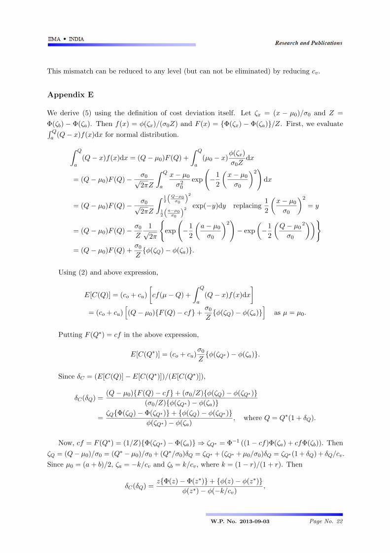
Appendix E

We derive (5) using the definition of cost deviation itself. Let ζx = (x − µ0)/σ0 and Z =

Φ(ζb) − Φ(ζa). Then f(x) = φ(ζx)/(σ0Z) and F (x) = {Φ(ζx) − Φ(ζa)}/Z. First, we evaluate∫ Qa (Q− x)f(x)dx for normal distribution.

∫ Q

a(Q− x)f(x)dx = (Q− µ0)F (Q) +

∫ Q

a(µ0 − x)

φ(ζx)

σ0Zdx

= (Q− µ0)F (Q)− σ0√2πZ

∫ Q

a

x− µ0

σ20

exp

(−1

2

(x− µ0

σ0

)2)

dx

= (Q− µ0)F (Q)− σ0√2πZ

∫ 12

(Q−µ0σ0

)2

12

(a−µ0σ0

)2exp(−y)dy replacing

1

2

(x− µ0

σ0

)2

= y

= (Q− µ0)F (Q)− σ0

Z

1√2π

{exp

(−1

2

(a− µ0

σ0

)2)− exp

(−1

2

(Q− µ0

σ0

2))}= (Q− µ0)F (Q) +

σ0

Z{φ(ζQ)− φ(ζa)}.

Using (2) and above expression,

E[C(Q)] = (co + cu)

[cf(µ−Q) +

∫ Q

a(Q− x)f(x)dx

]= (co + cu)

[(Q− µ0){F (Q)− cf}+

σ0

Z{φ(ζQ)− φ(ζa)}

]as µ = µ0.

Putting F (Q∗) = cf in the above expression,

E[C(Q∗)] = (co + cu)σ0

Z{φ(ζQ∗)− φ(ζa)}.

Since δC = (E[C(Q)]− E[C(Q∗)])/(E[C(Q∗)]),

δC(δQ) =(Q− µ0){F (Q)− cf}+ (σ0/Z){φ(ζQ)− φ(ζQ∗)}

(σ0/Z){φ(ζQ∗)− φ(ζa)}

=ζQ{Φ(ζQ)− Φ(ζQ∗)}+ {φ(ζQ)− φ(ζQ∗)}

φ(ζQ∗)− φ(ζa), where Q = Q∗(1 + δQ).

Now, cf = F (Q∗) = (1/Z){Φ(ζQ∗)− Φ(ζa)} ⇒ ζQ∗ = Φ−1 ((1− cf)Φ(ζa) + cfΦ(ζb)). Then

ζQ = (Q− µ0)/σ0 = (Q∗ − µ0)/σ0 + (Q∗/σ0)δQ = ζQ∗ + (ζQ∗ + µ0/σ0)δQ = ζQ∗(1 + δQ) + δQ/cv.

Since µ0 = (a+ b)/2, ζa = −k/cv and ζb = k/cv, where k = (1− r)/(1 + r). Then

δC(δQ) =z{Φ(z)− Φ(z∗)}+ {φ(z)− φ(z∗)}

φ(z∗)− φ(−k/cv),

W.P. No. 2013-09-03 Page No. 22

where z∗ = Φ−1 ((1− cf)Φ(−k/cv) + cfΦ(k/cv)) and z = z∗(1 + δQ) + δQ/cv.

Appendix F

For uniformly distributed demand, F (x) = (x− a)/(b− a). Using (4),

δC(δQ) =

∫ QQ∗{(x− a)/(b− a)− cf}dx

{(a+ b)/2−Q∗}cf +∫ Q∗a (x− a)/(b− a)dx

, where Q = Q∗(1 + δQ)

=

∫ QQ∗(x−Q

∗)/(b− a)dx

(1/2− cf)(b− a)cf +∫ Q∗a (x− a)/(b− a)dx

as cf = (Q∗ − a)/(b− a)

=(Q−Q∗)2/2

cf(1/2− cf)(b− a)2 + (Q∗ − a)2/2={a+ cf(b− a)}2

cf(1− cf)(b− a)2δ2Q.

Dividing the numerator and the denominator by b, we get (6).

References

Borgonovo, E., & Peccati, L. (2007). Global sensitivity analysis in inventory management.

International Journal of Production Economics, 108 (1-2), 302–313.

Bozarth, C. C., & Handfield, R. B. (2006). Introduction to Operations and Supply Chain

Management (1st ed.). Prentice Hall.

Chen, F., & Zheng, Y.-S. (1997). Sensitivity analysis of an (s,S) inventory model. Operations

Research Letters, 21 (1), 19–23.

Chen, L.-H., & Chen, Y.-C. (2010). A multiple-item budget-constraint newsboy problem with a

reservation policy. Omega, 38 (6), 431–439.

Choi, T.-M. (Ed.). (2012). Handbook of Newsvendor Problems (1st ed.). Springer.

Dobson, G. (1988). Sensitivity of the EOQ model to parameter estimates. Operations Research,

36 (4), 570–574.

Eeckhoudt, L., Gollier, C., & Schlesinger, H. (1995). The risk-averse (and prudent) newsboy.

Management Science, 41 (5), 786–794.

Gerchak, Y., & Mossman, D. (1992). On the effect of demand randomness on inventories and

costs. Operations Research, 40 (4), 804–807.

Gkedenko, B. V., & Kolmogorov, A. N. (1954). Limit Distributions for Sums of Independent

Random Variables (English translation by K. L. Chung). Massachusetts: Addison-Wesley

Publishing Company.

W.P. No. 2013-09-03 Page No. 23

Kevork, I. S. (2010). Estimating the optimal order quantity and the maximum expected profit

for single-period inventory decisions. Omega, 38 (3-4), 218–227.

Khouja, M. (1999). The single-period (news-vendor) problem: Literature review and suggestions

for future research. Omega, 27 (5), 537–553.

Lau, A. H.-L., & Lau, H.-S. (2002). The effects of reducing demand uncertainty in a manufacturer-

retailer channel for single-period products. Computers & Operations Research, 29 (11), 1583–

1602.

Lowe, T. J., & Schwarz, L. B. (1983). Parameter estimation for the EOQ lot-size model:

Minimax and expected value choices. Naval Research Logistics Quarterly , 30 (2), 367–376.

Lowe, T. J., Schwarz, L. B., & McGavin, E. J. (1988). The determination of optimal base-stock

inventory policy when the costs of under- and oversupply are uncertain. Naval Research

Logistics, 35 (4), 539–554.

Nahmias, S. (2001). Production and Operations Analysis (4th ed.). Boston: McGraw-Hill.

Porteus, E. L. (1990). Stochastic inventory theory. In D. P. Heyman & M. J. Sobel (Eds.),

Handbooks in or & ms, vol. 2 (pp. 610–628). Amsterdam: North-Holland Pub. Co.

Prichard, J. W., & Eagle, R. H. (1965). Modern Inventory Management (1st ed.). New York:

John Wiley & Sons.

Qin, Y., Wang, R., Vakharia, A. J., Chen, Y., & Seref, M. M. H. (2011). The newsvendor

problem: Review and directions for future research. European Journal of Operational Research,

213 (2), 361–374.

Ridder, A., van der Laan, E., & Salomon, M. (1998). How larger demand variability may lead

to lower costs in the newsvendor problem. Operations Research, 46 (6), 934–936.

Schweitzer, M. E., & Cachon, G. P. (2000). Decision bias in the newsvendor problem with a

known demand distribution: Experimental evidence. Management Science, 46 (3), 404–420.

Silver, E. A., Pyke, D. F., & Peterson, R. (1998). Inventory Management and Production

Planning and Scheduling (3rd ed.). New York: John Wiley & Sons.

Zheng, Y.-S. (1992). On properties of stochastic inventory systems. Management Science, 38 (1),

87–103.

W.P. No. 2013-09-03 Page No. 24