semi-quantitative evaluation of access and …...semi-quantitative evaluation of access and coverage...

Semi-Quantitative Evaluation of Access and Coverage (SQUEAC)/ Simplified Lot Quality Assurance Sampling Evaluation of Access and Coverage (SLEAC) Technical Reference

Mark Myatt, Brixton HealthErnest Guevarra, Valid InternationalLionella Fieschi, Valid InternationalAllison Norris, Valid InternationalSaul Guerrero, Action Against Hunger UKLilly Schofield, Concern WorldwideDaniel Jones, Valid InternationalEphrem Emru, Valid InternationalKate Sadler, Tufts University

October 2012

FANTAFHI 3601825 Connecticut Ave., NW Washington, DC 20009-5721Tel: 202-884-8000 Fax: 202-884-8432 [email protected] www.fantaproject.org THE SCIENCE OF

IMPROVING LIVES

Semi-Quantitative Evaluation of Access and Coverage (SQUEAC)/ Simplified Lot Quality Assurance Sampling Evaluation of Access and Coverage (SLEAC) Technical Reference Mark Myatt, Brixton HealthErnest Guevarra, Valid InternationalLionella Fieschi, Valid InternationalAllison Norris, Valid InternationalSaul Guerrero, Action Against Hunger UKLilly Schofield, Concern WorldwideDaniel Jones, Valid InternationalEphrem Emru, Valid InternationalKate Sadler, Tufts University October 2012

Food and Nutrition Technical Assistance III Project (FANTA)FHI 360 1825 Connecticut Avenue, NW Washington, DC 20009-5721 Tel: 202-884-8000 Fax: 202-884-8432 [email protected] www.fantaproject.org

This document was made possible by the generous support of the American people through the support of the U.S. Agency for International Development’s (USAID) Bureau for Global Health, Office of Health, Infectious Diseases, and Nutrition; Bureau for Democracy, Conflict, and Humanitarian Assistance, Office of U.S. Foreign Disaster Assistance; and USAID/Ghana, under terms of Cooperative Agreement No. GHN-A-00-08-00001-00 through the Food and Nutrition Technical Assistance II Project (FANTA-2), Cooperative Agreement No. AID-OAA-A-11-00014 through the FANTA-2 Bridge, and Cooperative Agreement No. GHN-A-00-08-00001-00 through FANTA III, all managed by FHI 360.

The contents are the responsibility of FHI 360 and do not necessarily reflect the views of USAID or the United States Government.

Recommended citation:

Myatt, Mark et al. 2012. Semi-Quantitative Evaluation of Access and Coverage (SQUEAC)/Simplified Lot Quality Assurance Sampling Evaluation of Access and Coverage (SLEAC) Technical Reference. Washington, DC: FHI 360/FANTA.

Contact information:

Food and Nutrition Technical Assistance III Project (FANTA)FHI 3601825 Connecticut Avenue, NWWashington, DC 20009-5721Tel: 202-884-8000Fax: [email protected]

AcknowledgementsThe authors wish to gratefully acknowledge the assistance of Megan Deitchler and Diana Stukel of the Food and Nutrition Technical Assistance Project (FANTA) for their invaluable technical advice.

SQUEAC/SLEAC Technical Reference i

ForewordDuring the past 10 years, the management of acute malnutrition has undergone a major paradigm shift that has changed the previous inpatient ‘clinical’ model of care into a community-based ‘public health’ model of care. Since 2007, this new model, called Community-Based Management of Acute Malnutrition (CMAM), has expanded rapidly and is now implemented in more than 55 countries worldwide.

In the old clinical model, the main determinant of impact was the quality of the inpatient medical and nutritional care provided in the centres and hospitals. By contrast, in the CMAM model, the key determinants of impact are the degree to which interventions treat people early in the course of their disease and the ability to treat as many of those affected as possible. This is a profound shift that requires an equivalent change in the protocols and indicators used to implement and monitor programs. Previously in the clinical model, impact was achieved using in-depth medical and nutritional protocols and results were monitored using clinicsimplicity and robustness of the CMAM treatment protocols

al outcomes indicators. Now, the are such that, as long as the basics such

as ready-to-use therapeutic food (RUTF) are available and those afflicted by acute malnutrition present early and in sufficient numbers, impact is ensured. In the new CMAM public health model, the focus on clinical guidelines has been replaced by protocols to ensure that those that are affected are admitted into programs early and the clinical outcome indicators have been supplemented by the direct assessment and monitoring of coverage.

The semi-quantitative evaluation of access and coverage (SQUEAC) and the simplified lot quality assurance sampling evaluation of access and coverage (SLEAC) assessment methods are an exciting new set of tools that draw together access and coverage, the two essential determinants of quality CMAM programming. SQUEAC combines an array of qualitative information about access and the perceptions of CMAM programs with small-sample quantitative surveys. These surveys test hypotheses generated during the qualitative work and establish levels of program coverage in key geographical areas. This combination both identifies key issues affecting presentation and program uptake whilst also establishing the actual levels of coverage attained. Vitally, all this can be done in real time, allowing the tool to be of immediate practical use to tweak program design and implementation in response to the information obtained.

The keys to the success of SQUEAC are diversity, triangulation, and iteration, which gradually build up a picture of the ‘truth’ about program coverage whilst simultaneously indicating what practical measures can be undertaken to improve access and coverage. The beauty of the technique is that it combines information that is often routinely collected but rarely used with other data specifically collected by fast, low-resource methods. Directly harnessing existing routine monitoring data to improve impact and program effectiveness greatly increases the cost efficiency of the additional time spent collecting new data, thereby decreasing the time and resource overhead required to implement SQUEAC.

SLEAC is a simple, low-cost, small-sample quantitative method. The keys to the success of SLEAC are simplicity, low cost, and versatility. SLEAC has the ability to map and estimate coverage over large areas.

As CMAM shifts from a donor-funded emergency intervention to a routine part of primary health-care programming, the resources available to implement these programs will inevitably decrease. In this environment, low-resource methods to increase timely access, monitor coverage, and allow program design to be proactively refined are essential if CMAM is to maintain its effectiveness. In my opinion, SQUEAC and SLEAC are major steps forward toward achieving these goals.

Steve CollinsMarch 2012

SQUEAC/SLEAC Technical Reference iii

Table of ContentsAcknowledgements..................................................................................................................................................iForeword................................................................................................................................................................iii

INTRODUCTION............................................................................................................................................................1Why Coverage Is Important....................................................................................................................................4

THE SQUEAC METHOD.................................................................................................................................................9Diverse Tools and Analyses...................................................................................................................................11Data Sources and Methods of Analysis: Routine Program Data...........................................................................12Information Provided by Routine Program Data...................................................................................................46Data Sources and Methods of Analysis: Qualitative Data.....................................................................................46Methods of Collecting Qualitative Data: Semi-Structured Interviews..................................................................47Methods of Collecting Qualitative Data: Simple Structured Interviews...............................................................50Methods of Collecting Qualitative Data: Informal Group Discussions..................................................................50Validating and Analysing Qualitative Data............................................................................................................50Storing, Organising, and Analysing Findings.........................................................................................................53Combining and Confirming Findings from Routine Program and Qualitative Data..............................................63Data Sources and Methods of Analysis.................................................................................................................68Using SQUEAC Data to Estimate Overall Program Coverage.................................................................................73An Example Conjugate Analysis............................................................................................................................85Beta-Binomial Conjugate Analysis Software.........................................................................................................88Diagnosing Coverage Estimates............................................................................................................................91Likelihood Surveys: Sampling and Sample Size.....................................................................................................93SQUEAC Survey Sample Size Example.................................................................................................................100A Note on Generating Random Numbers...........................................................................................................103Coverage Estimators...........................................................................................................................................104Reporting Overall Coverage Estimates................................................................................................................106Application of the SQUEAC Method...................................................................................................................110Clinical Audit, SQUEAC, and the Observer Effect................................................................................................112Conclusions.........................................................................................................................................................113

THE SLEAC METHOD.................................................................................................................................................114Classifying Program Coverage.............................................................................................................................117SLEAC Survey Sample Design..............................................................................................................................117SLEAC Survey Sample Size...................................................................................................................................118Classifying Coverage in Individual Service Delivery Units...................................................................................121Extending the Classification Method to Yield Finer Classifications.....................................................................122Estimating Coverage over Wide Areas................................................................................................................127Conclusions.........................................................................................................................................................133

SQUEAC AND SLEAC CASE STUDIES..........................................................................................................................134Case Study: Defining a Prior for Very High Coverage Programs..........................................................................134Case Study: Defining a Prior for Moderate Coverage Programs.........................................................................141Case Study: Defining a Prior by Wishful Thinking...............................................................................................148Case Study: Sampling without Maps or Lists......................................................................................................154Case Study: Using Satellite Imagery to Assist Sampling in Urban Settings.........................................................157Case Study: Active and Adaptive Case-Finding in a Rural Setting.......................................................................166Case Study: Within-Community Sampling in an Internally Displaced Persons Camp.........................................171Case Study: Within-Community Sampling in Urban Settings..............................................................................174Case Study: The Case of the Hidden Defaulters..................................................................................................178Case Study: Applying SLEAC: Sierra Leone National Coverage Survey................................................................182

APPENDIX 1. TECHNICAL APPENDIX.........................................................................................................................190APPENDIX 2. WORKING WITH FORMULAS...............................................................................................................207APPENDIX 3. GLOSSARY OF TERMS..........................................................................................................................211

SQUEAC/SLEAC Technical Reference v

List of Figures, Boxes, and TablesLIST OF FIGURES

Figure 1. Map showing the spatial distribution of point and period coverage in a CMAM program......................2Figure 2. Barriers to service access and uptake in a CMAM program reported by carers of non-covered cases....3Figure 3. Relations between factors influencing coverage and effectiveness.........................................................5Figure 4. Effect of coverage on met need in two programs....................................................................................7Figure 5. Tanahashi coverage diagram illustrating the effect of different types coverage barrier on service

achievement (met need)..........................................................................................................................8Figure 6. Complete seasonal calendar from a rapid rural appraisal (RRA) of a peasant association in Wollo,

Ethiopia..................................................................................................................................................10Figure 7. Plot of program admissions over time (with and without smoothing)..................................................13Figure 8. Admissions to a CMAM program over 6 years (with and without smoothing)......................................14Figure 9. Pattern of admissions over time over an entire program cycle for an emergency-response CMAM

program..................................................................................................................................................15Figure 10. Admissions over time in an emergency-response CMAM program with initially poor community

mobilisation...........................................................................................................................................15Figure 11. An example data collection form for collecting seasonal calendar data................................................16Figure 12. Pattern of CMAM admissions over time with seasonal calendars of human diseases associated

with SAM in children and household food availability...........................................................................17Figure 13. An example of a cycle of negative feedback (‘vicious circle’) associated with late presentation and

admission...............................................................................................................................................18Figure 14. Admission MUAC tabulated/plotted by hand using a tally sheet for a CMAM program admitting on

MUAC < 115 mm....................................................................................................................................19Figure 15. Admission MUAC plotted using a statistics package for a CMAM program admitting on

MUAC < 110 mm....................................................................................................................................20Figure 16. Admission MUAC in two programs admitting on MUAC < 115 mm.......................................................21Figure 17. Tally sheet showing an analysis of the duration of treatment episodes................................................23Figure 18. Standard therapeutic feeding program indicator graph.........................................................................25Figure 19. Pattern of defaulting rates over time with a seasonal calendar of household labour demand.............26Figure 20. Tally plot of number of visits before defaulting.....................................................................................27Figure 21. Home locations of program beneficiaries..............................................................................................28Figure 22. Villages visited by program outreach workers in the previous 2 months..............................................29Figure 23. Dates of outreach visits against a complete list of villages....................................................................30Figure 24. Home locations of program beneficiaries that defaulted in the previous 2 months.............................31Figure 25. A coverage assessment worker mapping the home locations of program beneficiaries.......................32Figure 26. Time-to-travel plots for formal discharges and defaulters.....................................................................34Figure 27. Time-to-travel for active (currently treated) cases for a single program site in a rural CMAM

program..................................................................................................................................................35Figure 28. Expected and observed pattern for time-to-travel for active (currently treated) cases within the

intended catchment area of a program site in a rural CMAM program.................................................37Figure 29. Creating the expected pattern of time-to-travel for cases within the intended catchment area of a

program site in a rural CMAM program given data on population and prevalence...............................38Figure 30. Simple approach to estimating the distance that carers will walk to access services............................40Figure 31. Mapping probable catchment areas of program sites to produce a first map of program coverage.....42Figure 32. Triangulation by source and method used to produce the map shown in Figure 31.............................43Figure 33. Cloakroom ticket/raffle ticket referral slip.............................................................................................44Figure 34. Example analysis of referrals from a CBV...............................................................................................44Figure 35. DNA rates for cases referred in the previous 2 months.........................................................................45Figure 36. Triangulation of SQUEAC data................................................................................................................52Figure 37. An example of a concept-map using explicitly defined relationship types............................................55Figure 38. An example of a concept-map using explicitly defined relationship types and an explanatory

annotation..............................................................................................................................................56Figure 39. An example mind-map from a SQUEAC investigation............................................................................57Figure 40. A mind-map being developed during a SQUEAC investigation..............................................................58Figure 41. A completed SQUEAC mind-map (following from Figure 40).................................................................59Figure 42. A mind-map being edited using XMind..................................................................................................62

SQUEAC/SLEAC Technical Reference vi

Figure 43. Area of probable low coverage identified by mapping of home locations (shown), analysis of outreach activities, defaulter follow-up, and qualitative data...............................................................64

Figure 44. Data from the small-area survey of the area shown in Figure 43..........................................................66Figure 45. Barriers to service uptake found in a SQUEAC small-area survey..........................................................67Figure 46. Reasons for defaulting found in a small study in a program with unacceptably high levels of

defaulting...............................................................................................................................................69Figure 47. Simplified LQAS nomogram for finding d given n and p........................................................................71Figure 48. Binomial probability density for coverage from a survey of 20 SAM cases of which 10 cases were

covered..................................................................................................................................................75Figure 49. Prior information from a SQUEAC investigation grouped into positive and negative findings with

simple and weighted scores...................................................................................................................76Figure 50. Deciding the mode of the prior as the product of program performance at key processes

associate with program coverage..........................................................................................................78Figure 51. Steps in drawing a histogram prior........................................................................................................80Figure 52. The Beta(16.02, 13.65) prior..................................................................................................................82Figure 53. A plot of the example beta-binomial conjugate analysis.......................................................................87Figure 54. Pocket calculator with square-root function.........................................................................................88Figure 55. The example beta-binomial conjugate analysis using BayesSQUEAC.................................................89Figure 56. Using BayesSQUEAC to calculate the sample size required to estimate coverage with a

precision of ± 10% using a Beta(29, 13) prior using the simulation approach.......................................90Figure 57. Illustration of the effect of the strength and accuracy of three different priors on the posterior

coverage estimate in a population with true coverage of 28% with identical likelihoods.....................92Figure 58. A coarse CSAS/quadrat sample of villages.............................................................................................94Figure 59. A finer and wider CSAS/quadrat sample of villages than in Figure 58...................................................95Figure 60. Villages selected using stratified systematic sampling...........................................................................96Figure 61. Selection of villages to be sampled using CSAS sampling....................................................................101Figure 62. Selection of villages to be sampled using spatially stratified sampling...............................................102Figure 63. Distribution of per-quadrat point coverage found by the survey reported in Figure 1.......................107Figure 64. Map of per-quadrat point coverage calculated using likelihood survey data......................................108Figure 65. Coverage over time..............................................................................................................................109Figure 66. The clinical audit cycle.........................................................................................................................110Figure 67. Using SLEAC and SQUEAC in failing service delivery units...................................................................115Figure 68. Using SLEAC and SQUEAC in succeeding and failing service delivery units ........................................115Figure 69. The level of mapping available from SLEAC and CSAS methods..........................................................116Figure 70. Algorithm for a three-class simplified LQAS classifier..........................................................................122Figure 71. Simplified LQAS nomogram for finding appropriate values for d1 and d2 given n, p1, and p2...........124Figure 72. Finding suitable αPrior and βPrior parameters for the prior using BayesSQUEAC.................................137Figure 73. Finding the likelihood survey sample size by simulation using BayesSQUEAC.................................138Figure 74. Grid (CSAS) sample used for the likelihood survey..............................................................................139Figure 75. Estimating period coverage using BayesSQUEAC.............................................................................141Figure 76. Simplified mind-map for the SQUEAC investigation findings...............................................................142Figure 77. Building the histogram prior................................................................................................................145Figure 78. A prior that is not symmetrical about the mode.................................................................................146Figure 79. Beta(15.4, 15.4) prior matching the histogram prior developed in Figure 78.....................................147Figure 80. Simplified mind-map of SQUEAC findings............................................................................................149Figure 81. The prior selected by the survey team................................................................................................150Figure 82. The prior selected by the SQUEAC trainer...........................................................................................150Figure 83. Results of the beta-binomial conjugate analysis performed with the team’s Beta(19, 24) prior

and the SQUEAC trainer’s Beta(7, 35) prior.........................................................................................152Figure 84. The most ‘detailed’ map available.......................................................................................................154Figure 85. The list of villages was sorted by sub-district and parish.....................................................................155Figure 86. Calculating a minimum sample size using the BayesSQUEAC calculator........................................158Figure 87. District boundaries marked on a low-resolution satellite image.........................................................160Figure 88. District boundary of Shingani district marked on a satellite image.....................................................160Figure 89. Sub-district boundaries added to the satellite image of Shingani district...........................................161Figure 90. Rough hand-drawn map use to create lists of locations by sub-district..............................................162Figure 91. Location boundaries added to the satellite image of Shingani district................................................162

SQUEAC/SLEAC Technical Reference vii

Figure 92. List of locations sorted by district and sub-district created from the mapping process (also showing systematic sampling with start = 3 and interval = 9).................................................163

Figure 93. Locations in Shingani district selected for sampling.........................................................................164Figure 94. Satellite image showing a single sampling location..........................................................................165Figure 95. The survey process using active and adaptive case-finding.............................................................169Figure 96. The Beta(12.9, 12.3) prior in BayesSQUEAC.................................................................................174Figure 97. Administrative hierarchy of the city.................................................................................................175Figure 98. Sample size by simulation approach using BayesSQUEAC............................................................175Figure 99. The conjugate analysis in BayesSQUEAC.......................................................................................177Figure 100. Number of visits before defaulting...................................................................................................179Figure 101. Trend of defaulting over time...........................................................................................................180Figure 102. Distance from home to a CMAM program site for active cases and defaulters...............................181Figure 103. Structure of samples in rural and peri-urban/urban districts...........................................................182Figure 104. Example of a large-scale map showing enumeration area boundaries used when sampling in an

urban district....................................................................................................................................184Figure 105. Map of per-district coverage............................................................................................................187Figure 106. Barriers to service uptake and access...............................................................................................188Figure 107. Calculation of a wide-area coverage estimate..................................................................................189Figure A1-1. Sample size calculation by simulation using BayesSQUEAC.........................................................193Figure A1-2. Uncertainty/precision associated with sample sizes between 34 and 68 over the typical range

of coverages achieved by CMAM programs ....................................................................................194Figure A1-3. Normal approximation to Beta(α, β) distributions with two different modes and different

values of α and β.............................................................................................................................196Figure A1-4. Operating characteristic and probability of classification plots found from simulations of

two-class and three-class SLEAC methods with n = 40....................................................................203Figure A1-5. Programming a spreadsheet for three different moving averages with a span of three

successive data points.....................................................................................................................204Figure A1-6. Effects of moving average smoothers of spans 3 (M3A3) and 13 (M13A13) on 6 years of

monthly admissions data.................................................................................................................205Figure A1-7. Seasonal component of 6 years of monthly admissions data found by subtracting data

smoothed using M13A13 from data smoothed using M3A3...........................................................206

LIST OF TABLESTable 1. Use of a table to investigate the effect of distance on admissions and defaulting in the previous

month in a single clinic catchment area................................................................................................32Table 2. Using lists to identify locations where coverage is likely to be poor or defaulting is likely to be high. .33Table 3. A data collection plan for triangulation by source and method of data regarding seasonal

calendars of disease, labour demand, and food availability.................................................................51Table 4. Approximate values for αPrior and βPrior for different prior modes at two different levels of

uncertainty............................................................................................................................................83Table 5. Target sample sizes for 50% and 70% coverage standards for use when surveying small service

delivery units and/or the prevalence of SAM is low............................................................................118Table 6. Critical values of the chi-square test statistic......................................................................................132Table 7. Summary of the findings of the initial SQUEAC assessment...............................................................135Table 8. Summary of the assessed effects of the identified barriers................................................................136Table 9. Boosters and barriers to coverage found in the SQUEAC investigation...............................................143Table 10. Ranking and weighting of boosters and barriers to find a credible prior mode..................................144Table 11. Coverage classification by district.......................................................................................................186Table A1-1. Finding a sample size for a desired precision using simulation and a simple directed search

strategy............................................................................................................................................192Table A2-1. Operators used in SQUEAC and SLEAC formulas..............................................................................208

LIST OF BOXESBox 1. Example interview guide for first interviews with carers of children in a program..............................48Box 2. Simple structured interview questionnaire to be applied to carers of non-covered cases...................49Box 3. Active and adaptive case-finding..........................................................................................................65Box 4. Using BayesSQUEAC to find α and β values that match a histogram prior....................................157

SQUEAC/SLEAC Technical Reference viii

IntroductionOne of the most important elements behind the success of the Community-Based Management of Acute Malnutrition (CMAM) model of service delivery is its proven capacity for achieving and sustaining high levels of coverage over wide areas.

Two-stage cluster sampled surveys have been used to estimate the coverage of selective feeding programs. This approach suffers from several important limitations. In response, Valid InternationalConcern Worldwide, and the Food and Nutrition Technical Assistance Project (FANTA) developed new survey method for estimating the coverage of selective feeding programs. This survey method, known as the Centric Systematic Area Sampling (CSAS) method, uses a combination of stratified and systematic area sampling and active and adaptive case-finding.

The CSAS survey method provides a rich set of information about program coverage. In particular, provides a ‘headline’ estimate of overall program coverage, a map of the spatial distribution of program coverage (Figure 1), and a ranked list of program-specific barriers to service access and uptake (Figure 2).

The CSAS method is, however, resource intensive. This has led to a tendency for it to be used for program evaluation rather than for day-to-day program planning and program monitoring purposesThe results of CSAS surveys have, therefore, often been able to explain why a particular program failed to achieve a satisfactory level and spatial pattern of coverage, but this information has tended to arrive too late in the program cycle to institute effective remedial action.

The CMAM model of service delivery is now being adopted in developmental and post-emergency settings. Programs in these settings tend to suffer from considerable resource scarcity compared to emergency-response programs implemented by non-governmental organisations (NGOs). There exists, therefore, a need for low-resource methods capable of evaluating program coverage, identifying barriers to service access and uptake, and identifying appropriate actions for improving access and program coverage. This document describes two such methods – the semi-quantitative evaluation of access and coverage (SQUEAC) method and the simplified Lot Quality Assurance Sampling evaluation of access and coverage (SLEAC) method – and how they can be used to investigate and improve three aspects of CMAM programs: effectiveness, coverage, and ability to meet need.

, a

it

.

SQUEAC/SLEAC Technical Reference 1

Figure 1. Map showing the spatial distribution of point and period coverage in a CMAM program

District boundary

Major road

Towns and villages

Program site

Legend

Left-hand bar represents pointcoverage on a scale of 0% to 100%

Right-hand bar represents periodcoverage on a scale of 0% to 100%

Data courtesy of Save the Children/United Kingdom


Figure 2. Barriers to service access and uptake in a CMAM program reported by carers of non-covered cases

Fear of rejection

Child not recognised as 'malnourished'

Program site too far away

Lack of program information

Relapse or deafult (not returned)

Other reasons

Inappropriately discharged

Interface problems

0 10 20 30 40 50 60 70 80

Number of non-covered cases

Data courtesy of Save the Children/United Kingdom

Note: This type of graph is most effective when you have a limited number (e.g., ≤ 10) of barriers to report. Similar barriers should be grouped together. For example, the barriers:

Carer not aware of program

Carer did not know location of program site

Carer did not know that the program site provided RUTF

could be merged into a single ‘Lack of knowledge about the program’ category.

Infrequently reported barriers should be grouped into a single ‘Other’ category. Pie charts should not be used to present this type of data.


Why Coverage Is Important

The efficacy of the CMAM protocol can be defined as how well the protocol works in ideal and controlled settings. It is measured by the cure rate:

Number CuredCureRate (%)= × 100

Number Treated

which is usually estimated in a clinical trial.

For the CMAM protocol, the cure rate is close to 100% in uncomplicated incident cases (i.e., in cases with mid-upper arm circumference [MUAC] at or just below the admission criteria and cases with mild oedema). There is, therefore, little room for large improvements in the efficacy of the CMAM protocol. Although we cannot significantly change the efficacy of the CMAM protocol, we can change the effectiveness of the CMAM protocol.

The effectiveness of the CMAM protocol can be defined as the cure rate in a beneficiary cohort under program conditions. Effectiveness depends, to a large extent, on:

Severity of disease. Early treatment seeking and timely case-finding and recruitment of severe acute malnutrition (SAM) cases will result in a beneficiary cohort in which the majority of cases are uncomplicated incident cases. The cure rate of the CMAM protocol in such a cohort is close to 100%. Late treatment seeking and weak case-finding and recruitment will result in a cohort of more severe and more complicated cases. The cure rate in such a cohort may be much lower than 100%.Compliance. Programs in which the beneficiary and the provider adhere strictly to the CMAM protocol have a better cure rate than programs in which adherence to the CMAM protocol is compromised. Poor compliance can be a problem with the beneficiary (e.g., sharing of ready-to-use therapeutic food [RUTF] within the household) or a problem with the provider (e.g., RUTF and drug stock-outs), and both have a negative impact on effectiveness.Defaulting. This is the ultimate in poor compliance.

An effective program must, therefore, have:Thorough case-finding and early treatment seeking. This ensures that the beneficiary cohort consists mainly of uncomplicated incident cases that can be cured quickly and cheaply.A high level of compliance. This ensures that the beneficiary receives a treatment of proven efficacy.Good retention from admission to cure (i.e., little or no defaulting). This also ensures that the beneficiary receives a treatment of proven efficacy.

Coverage is one factor (the other being effectiveness) in the capacity of a program to meet need. It can be expressed as:

Number in the programProgram Coverage (%)= × 100

Number who should be in the program

Coverage depends directly on:Thorough case-finding and early treatment seeking. This ensures that the majority of admissions are uncomplicated incident cases, which leads to good outcomes (i.e., close to 100% cure rate).Good retention from admission to cure. This is the absence of defaulting.

Coverage also indirectly depends on compliance (see Figure 3).


Figure 3. Relations between factors influencing coverage and effectiveness

EarlyAdmission

FewComplications

OutpatientCare

ShortStay

Low Levelsof Defaulting

GoodOutcomes

PositiveOpinions

GoodCompliance

encourages

leads to

associated with

allows

leads to

leads to

leads toleads to

leads to

associated with

leads to

encourages

CommunitySensitisation

encourages

CommunityMobilisation

ActiveCase-Finding

needed for needed for

EarlyTreatment

Seeking

leads to

leads to

leads to

leads to


Meeting need requires both high effectiveness and high coverage:

Met Need = Effectiveness × Coverage

Coverage and effectiveness depend on the same things (see Figure 3) and are linked to each other:

Effectiveness Coverage

Effective programs have high coverage

High coverage programs have high cure rates

Good coverage supports good effectiveness. Good effectiveness supports good coverage. Maximizing coverage maximises effectiveness and met need.

The implications of:

Met Need = Effectiveness × Coverage

are illustrated in Figure 4 and Figure 5. Programs with low coverage fail to meet need.


Figure 4. Effect of coverage on met need in two programs


Figure 5. Tanahashi coverage diagram illustrating the effect of different types coverage barrier on service achievement (met need)


TARGET POPULATION

AVAILABILITY COVERAGE

People for whom the service is available

ACCESSIBILITY COVERAGE

People that can use the service

ACCEPTIBILITY COVERAGE

People that are willing to use service

CONTACT COVERAGE

People that use the service

EFFECTIVENESS

People that receive effective care

GOAL OF SERVICE ACHIEVEMENT

OPERATION CURVE

Number of People

Proc

ess

of S

ervi

ce P

rovi

sion

CoverageBarriers

Effect of Coverage Barrierson Service Achievement

The following two sections describe the SQUEAC and SLEAC methods for investigating and improving the coverage, effectiveness, and met need of CMAM programs. These sections are followed by 10 case studies, each of which presents useful insights into how SQUEAC and SLEAC can and should be applied; a technical appendix, which provides greater detail about case-finding, survey sample sizes, calculations used in SQUEAC and SLEAC, and smoothing of time-series data; a brief tutorial on working with the formulas used in this document; and a glossary of SQUEAC and SLEAC terms.

The SQUEAC MethodSQUEAC is a coverage assessment method developed by Valid International, FHI 360/FANTA, UNICEF, Concern Worldwide, World Vision International, Action Against Hunger, Tufts University, and Brixton Health.

After discussions with implementing partners in the NGO, U.N., and government sectors, the following attributes were considered important:

• The method must be both quick and cheap to allow frequent and ongoing evaluation of program coverage and identification of barriers to service access and uptake.

• The method must provide a similar richness of information as that provided by the CSAS method, including:

• Evaluation of the spatial pattern of coverage• Identification of barriers to service access and uptake

• Estimation of overall program coverage was considered to be desirable but not essential.• The method should encourage the routine collection, analysis, and use of program planning

and evaluation data.• Individual components of the method should provide information capable of informing

program activities and reforms.• The method should not require the use of computers.

The SQUEAC method presented here:

• Is semi-quantitative, using a mixture of quantitative (numerical) data collected from routine program monitoring activities, small studies, small surveys, and small-area surveys, as well as qualitative data collected using informal group discussions and interviews with a variety of informants.

• Makes use of routine program monitoring data (e.g., charts of trends in admission, exit, recovery, in-program deaths, and defaulting) and data that are already collected on beneficiary record cards (e.g., admission MUAC and the home villages of program beneficiaries).

• Makes use of data such as agriculture, labour, disease, and food-consumption calendars as well as market price monitoring data that might already be available from such sources as nutritional anthropometry surveys, agricultural assessments, livelihood surveys, and food-security assessments (see Figure 6). When these data are not readily available, they may be collected using informal group discussions and interviews with a variety of informants.

• Makes use of data that may already be collected routinely by programs or may be collected with little additional work. These additional data have been selected to provide benefits to programs outside the narrow requirement of evaluating access and coverage.

• Uses small studies, small surveys, and small-area surveys to confirm or deny hypotheses about program coverage that arise from the analysis of program and qualitative data.

• Uses Bayesian techniques to estimate overall program coverage with a small-sample survey.

The SQUEAC method achieves rapidity and low cost by collecting and analysing diverse data intelligently, rather than by using the mechanistic and more focussed data collection and analysis techniques employed by the CSAS method.


Figure 6. Complete seasonal calendar from a rapid rural appraisal (RRA) of a peasant association in Wollo, Ethiopia

This seasonal calendar was adapted from:

McCracken, J.A.; Pretty, J.N.; and Conway, G.R. 1988. An introduction to rapid rural appraisal for agricultural development. London: International Institute for Environment and Development.

Data courtesy of the Ethiopian Red Cross Society


The SQUEAC method uses a two-stage screening test model:Stage 1 identifies areas of low and high coverage as well as reasons for coverage failure using routine program data, already available data, quantitative data that may be collected with little additional work, and qualitative data.Stage 2 confirms the location of areas of high and low coverage and the reasons for coverage failure identified in Stage 1 using small studies, small surveys, small-area surveys.

If appropriate and required, an additional stage may be performed:Stage 3 provides an estimate of overall program coverage using Bayesian techniques.

SQUEAC consists of a set of tools each of which is designed to identify and investigate coverage and factors influencing coverage.

The tools presented here have been developed and tested in use-studies and by SQUEAC practitioners that have undertaken more than 50 SQUEAC investigations of CMAM programs in many countries in Africa and Asia.

It is expected that new tools will be added and existing tools refined as practitioners gain more experience with the SQUEAC method. A SQUEAC investigation will typically use some (but not all) of the tools described here.

Diverse Tools and Analyses

SQUEAC relies on a diversity of analyses pursued through the use of diverse sources of information, diverse means of collecting information, and diverse methods of analysing information (triangulation). Accuracy and completeness are achieved by investigating coverage and factors influencing coverage in a variety of ways. The ‘truth’ about coverage is approached by a rapid and intelligent accumulation of diverse information, rather than by a single process of dumb statistical replication (although some dumb statistical replication will play a useful role in almost all SQUEAC investigations). Use of routine data, secondary data (e.g., from food-security assessments and nutritional anthropometry surveys), semi-structured interviews, case-histories, informal group discussions, small studies, small surveys, small-area surveys, and the preparation of maps and diagrams all contribute to a progressively accurate and complete analysis of program coverage.

SQUEAC is a semi-structured activity designed to rapidly accumulate new and relevant information about coverage and factors influencing coverage and to develop and test hypotheses about coverage and factors influencing coverage.


SQUEAC is:• Investigative. SQUEAC is not a survey technique. It is a technique for investigating

coverage and factors influencing coverage. A SQUEAC investigation will, if needed, include surveys, but should never be limited to undertaking surveys.

• Iterative. The process of a SQUEAC investigation is not fixed, but is modified as knowledge is acquired. This can be thought of as a process of ‘learning as you go’. New information is used to decide the next steps of the investigation.

• Innovative. There is no standardised SQUEAC method. SQUEAC is a set of tools for investigating coverage and factors influencing coverage. If, when, and how these tools are used depends on the particular setting and the skills of the investigator. Different tools may be used and new tools may be developed as required.

• Interactive. The method collects information through intelligent interaction with program staff, program beneficiaries, and community members using semi-structured interviews, case histories, and informal group discussions.

• Informal. The method uses informal but guided interview techniques as well as formal survey instruments to collect information about coverage and factors influencing coverage.

• In the community. Much of the information used in SQUEAC investigations is collected in the community through interaction with community members. SQUEAC lets you see your program as it is seen by the community.

• Intelligent. Triangulation is a purposeful and intelligent process. Data from different sources and methods are compared with each other. Discrepancies in the data are used to inform decisions about whether to collect further data. If further data collection is required, these discrepancies help determine which data to collect, as well as the sources and methods to be used to collect them.

When done correctly, a SQUEAC investigation will contain all these elements and provide useful information about coverage and factors influencing coverage.

Data Sources and Methods of Analysis: Routine Program Data

The most important item of routine program data is the number of admissions over time. This should be graphed with time on the x axis and number of admissions on the y axis. Since there is likely to be considerable weekly or monthly variation in the number of admissions it is advisable to apply some form of smoothing using, for example, the method of moving averages to the data (Figure 7 and Figure 8). Smoothing time-series data using moving averages is discussed in Appendix 1.

Experience with CMAM programs in a variety of emergency settings shows that programs with reasonable coverage display a distinctive pattern in the plot of admissions over time. Figure 9 shows this pattern over an entire program cycle for an emergency-response program. The number of admissions increases rapidly, falls slightly before stabilising, and finally drops away as the emergency abates and the program is scaled down and approaches closure. Major deviations from this pattern in the absence of evidence of mass migration or significant improvements in the health, nutrition, and food-security situation of the program’s target population indicates a potential problem with a program’s recruitment procedures. For example, Figure 10 shows a plot of admissions over time in an emergency-response CMAM program that had neglected to undertake effective community mobilisation and outreach activities. Admissions initially increased rapidly and then fell away rapidly. Such a pattern is indicative of a program with limited spatial coverage relying on self-referrals. An acceptable pattern was established in this program after effective remedial action was undertaken.


The pattern of admissions in a non-emergency setting is likely to be more complicated and, once the program has been established, should vary with the incidence of SAM in the program’s catchment area (e.g., as in Figure 8). Making sense of the plot of admissions over time in such settings requires information about the probable or expected incidence of SAM. This can be determined using seasonal calendars of human diseases associated with SAM in children (e.g., diarrhoea, fever, and acute respiratory tract infection) and food availability. This information may be available from health and nutrition or food-security assessments (e.g., as in Figure 6). If this information is not already available, it should be collected at the start of the program or during the SQUEAC investigation. Figure 11 shows an example data collection form. Prevalence and incidence data may be available from previous nutritional anthropometry surveys, surveillance systems, and clinic workload returns. Figure 12, for example, shows a plot of admissions over time with seasonal calendars of human diseases and food availability. The pattern of the plot of admissions over time conforms to expectations (i.e., the program treated more cases at times when the incidence of SAM was likely to be high). Deviation from the expected pattern indicates a potential problem with a program’s recruitment procedures.

Figure 7. Plot of program admissions over time (with and without smoothing)


Raw data smoothed using moving medians of span = 3 followed by moving averages of span = 3.

Data courtesy of Concern Worldwide

0 1 2 3 4 5 6 7 8 9 10 11 12 13 14 15 16 17 18 19 20

50

75

100

125

150

Months since start of program

Ad

mis

sion

s

Figure 8. Admissions to a CMAM program over 6 years (with and without smoothing)

M3A3: Raw data smoothed using moving medians of span = 3 followed by moving averages of span = 3 (showing seasonality and trend).M13A13: Raw data smoothed using moving medians of span = 13 followed by moving averages of span = 13 (showing trend only).

Data courtesy of Brixton Health


Figure 9. Pattern of admissions over time over an entire program cycle for an emergency-response CMAM program

Time

Figure 10. Admissions over time in an emergency-response CMAM program with initially poor community mobilisation


Time

Figure 11. An example data collection form for collecting seasonal calendar data

Data courtesy of UNICEF Sudan


Figure 12. Pattern of CMAM admissions over time with seasonal calendars of human diseases associated with SAM in children and household food availability


Time

Num

ber

of n

ew

ad

mis

sio

ns

Diarrhoea

ARI

Fever Fever

ARI

Fever

Dis

eas

e

Diarrhoea

Foo

d e

ate

n

Plotting admissions over time is useful but ignores the issue of the timeliness of admissions. Children with MUAC below program admission criteria or with nutritional oedema should be in the program. If many of these children are not in the program then program coverage will be low. These children can be divided into two groups:

• Children that meet program admission criteria but never get admitted to the program. These children either recover outside of the program or die. It is possible to identify some of these children using referral monitoring or surveys.

• Children that are admitted to the program, but only after they have met program admission criteria for a considerable period of time. These children are late admissions and can be identified using data that are usually recorded on the beneficiary record card.

Late admissions are direct coverage failures (because they will have been non-covered SAM cases for a considerable period of time before admission) but they also affect coverage indirectly. Late admission is associated with the need for inpatient care, longer treatment, defaulting, and poor treatment outcomes (e.g., death). These can lead to poor opinions of the program circulating in the host population, which may lead to more late presentations and admissions and a cycle of negative feedback may develop (Figure 13).

Figure 13. An example of a cycle of negative feedback (‘vicious circle’) associated with late presentation and admission


Late admissions may be investigated by plotting MUAC at admission. Data can be tabulated and plotted by hand using a tally sheet (Figure 14) or using a spreadsheet, graphics, or statistics package (Figure 15). Summary measures may be calculated, but visual inspection and interpretation of the plot is usually more informative. A plot of admission MUAC from a program with high coverage is likely to have a very large number of admissions close to the program admission criteria, as in Figure 14, Figure 15, and Figure 16.A. Plots that differ markedly from this (e.g., as in Figure 16.B) are indicative of problems with case-finding and recruitment and low program coverage.

The interpretation of plots of admission MUAC should take into account the phase of the program being investigated. For example, during the start-up phase of a program, the plots of admission MUAC will usually look something like Figure 16.B. This is because, in the first few months of program operation, both prevalent cases (i.e., cases that have been SAM for some time and may have very low MUACs) and incident cases (i.e., cases that have only recently developed SAM and have MUACs close to the program admission criteria) are found and admitted. When investigating the coverage of an established program, it is often useful, therefore, to plot admission MUAC for recent program admissions only (e.g., admissions occurring in the previous 6 months).

Figure 14. Admission MUAC tabulated/plotted by hand using a tally sheet for a CMAM program admitting on MUAC < 115 mm

Data courtesy of World Vision International


Figure 15. Admission MUAC plotted using a statistics package for a CMAM program admitting on MUAC < 110 mm

Data courtesy of Save the Children (USA) and the Friedman School of Nutrition Science and Policy (Tufts University)


Figure 16. Admission MUAC in two programs admitting on MUAC < 115 mm


114 113 112 111 110 109 108 107 106 105 104 103 102 101 100 99 98 97 96 95 94 93 92 91 92 91 90 89

Admission MUAC

Num

ber

of a

dmis

sion

s

114 113 112 111 110 109 108 107 106 105 104 103 102 101 100 99 98 97 96 95 94 93 92 91 92 91 90 89

Admission MUAC

Num

ber

of a

dm

issi

ons

A : High-coverage program

B : Problems with case-finding and recruitment (low coverage) or new program

Another way of investigating late admissions is to calculate the proportion of program beneficiaries requiring inpatient care at admission:

Number of program beneficaries requiring inpatient care at admission × 100Total number of inpatient and outpatient admissions

Interpretation of the proportion of program beneficiaries requiring inpatient care at admission should also take into account the phase of the program being investigated. The proportion of program beneficiaries requiring inpatient care at admission is likely to be high during the start-up phase of a program. In an established program, however, the proportion of program admissions requiring inpatient care should not exceed 5%.

Note that the calculation of the proportion of program beneficiaries requiring inpatient care at admission uses the number of program beneficiaries requiring inpatient care at admission rather than the number of program beneficiaries admitted to inpatient care as the numerator. This is because many carers may not accept a referral to an inpatient facility.

The proportion of program beneficiaries requiring inpatient care at admission may also be analysed (classified) using the simplified Lot Quality Assurance Sampling (LQAS) classification technique presented later in this section.

An investigation of late admissions will usually identify some very late admissions (e.g., the three cases with MUAC < 90 mm in Figure 14). Children that remain untreated for such long periods with declining nutritional status should be treated as critical incidents. Investigation of critical incidents often reveals useful information about program performance. For example, a SQUEAC investigation of a CMAM program in Bangladesh reported:

A child was admitted to the program with a MUAC of 82 mm. The mother of this case had moved (within the program catchment area) to live with her father because of family problems. While at her grandfather’s house, the child developed diarrhoea with fever and rapid weight loss. The child spent 12 days in the local hospital before being discharged with a MUAC approaching 82 mm. The community nutrition volunteers at the grandfather’s home union and the mother’s home union were not informed by the hospital. Program staff were also not informed by the hospital. The case was, however, picked up by the community nutrition volunteer at the grandfather’s home union, referred to the community nutrition volunteer at the case’s home union, and admitted to the program. The referring community nutrition volunteer also informed program staff of the referral.

In this example, the investigation of a critical incident revealed good communications within the program but a problem with the interface between the local hospital and the program and prompted further investigation into the interface between the local hospital and the program.

Examining the duration of the treatment episode (i.e., the time from admission to discharge) may also provide useful information about program coverage. The duration of the treatment episode is sometimes called the ‘length of stay’.

Long treatment episodes may be due to late admission or poor adherence to the CMAM treatment protocol by program staff (e.g., failure to give a systemic antimicrobial, RUTF stock-outs) and beneficiaries (e.g., intra-household sharing of RUTF, lack of continuity of care). Programs with long treatment episodes tend to be unpopular with beneficiaries and suffer from late treatment seeking and high levels of defaulting (both of which are failures of coverage).


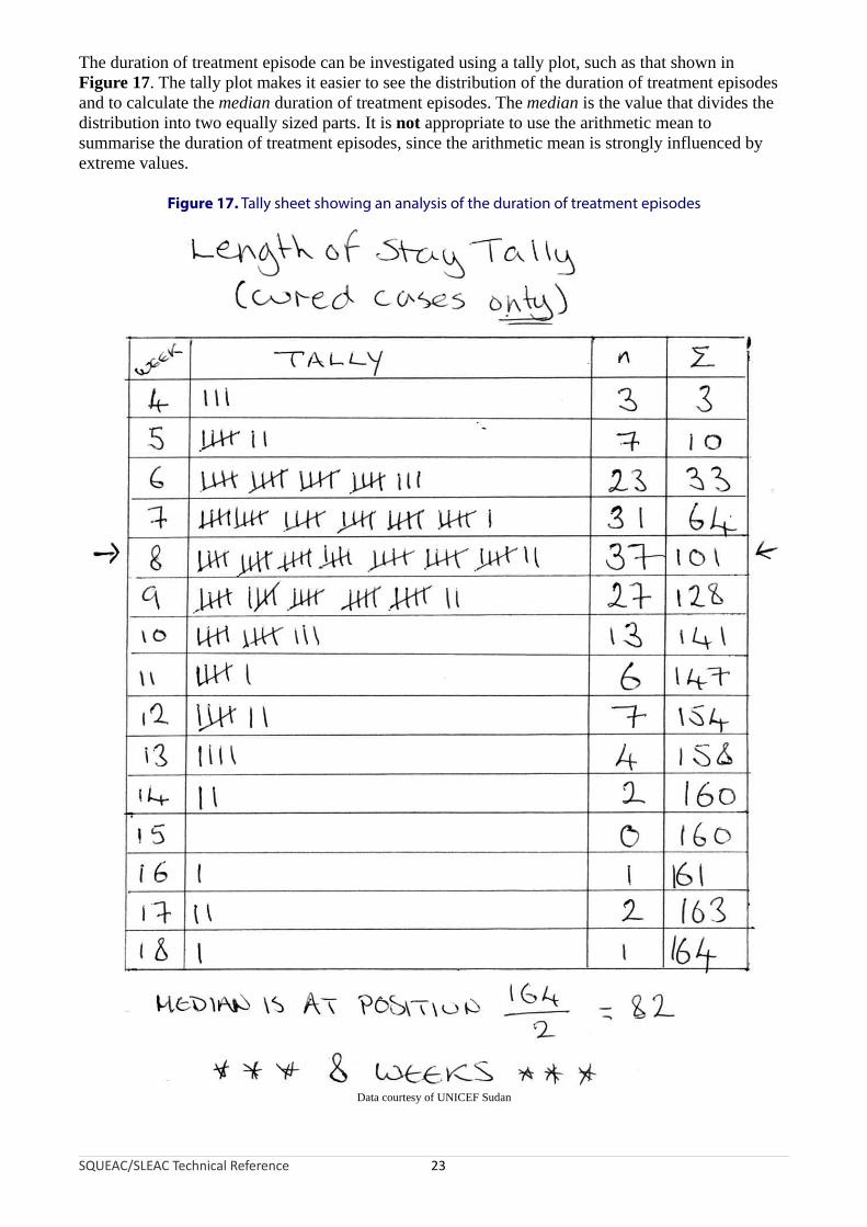
The duration of treatment episode can be investigated using a tally plot, such as that shown in Figure 17. The tally plot makes it easier to see the distribution of the duration of treatment episodes and to calculate the median duration of treatment episodes. The median is the value that divides the distribution into two equally sized parts. It is not appropriate to use the arithmetic mean to summarise the duration of treatment episodes, since the arithmetic mean is strongly influenced by extreme values.

Figure 17. Tally sheet showing an analysis of the duration of treatment episodes



Higher coverage programs tend to have a median duration of treatment episodes of less than or equal to about 8 weeks.

When examining the duration of treatment episodes you should restrict the analysis to planned discharges (i.e., include cases discharged as cured and as non-responders in the analysis, but exclude defaulters and transfers to other programs from the analysis). The analysis presented in Figure 17, for example, was restricted to cured cases only.

The interpretation of plots and summaries of duration of treatment episodes should take into account the phase of the program being investigated. For example, during the start-up phase of a program, there may be many long duration treatment episodes. This is because, in the first few months of program operation, both prevalent (old) and incident (new) cases are found and admitted. When investigating the coverage of an established program, it is often useful, therefore, to plot and summarise duration of treatment for recent discharges only (e.g., discharges occurring in the previous 6 months).

Plots of admissions over time and admission MUAC can reveal potential problems with a program’s recruitment procedures, but ignore the problem of defaulters. Defaulters are children that have been admitted to the program but leave the program without being formally discharged, without being transferred to another service, or without having died. Defaulters are, therefore, children that should be in the program but are not in the program. This means that high defaulting rates are associated with low program coverage. Standard program indicator graphs should show a consistently low rate of defaulting. Figure 18 shows a standard program indicator graph from a CMAM program. This graph shows an increasing defaulting rate. This was due to the program having too few sites. More cases were found and admitted as the program’s outreach activities were expanded, but more of these cases defaulted after the initial visit because beneficiaries and carers had to travel too far to access services. Note that deaths in Figure 18 show a similar pattern to defaulters. The bulk of these deaths were in late admissions from communities furthest from program sites.


Figure 18. Standard therapeutic feeding program indicator graph


In some programs, defaulting rates may vary over time. This will usually be due to a deterioration in the security situation, meteorological conditions (e.g., difficulties travelling in rainy or hot seasons), or patterns of labour demand. Figure 19, for example, shows a plot of the defaulting rate over time with a seasonal calendar of household labour demands. In this example, defaulting is associated with household labour demands. Such a problem could be corrected by reducing the cost of attendance by, for example, opening additional program sites, using mobile clinics, reducing contact frequency from weekly to fortnightly contact, or reducing waiting times at program sites. Plots of defaulting rates over time should present defaults as a proportion of all program exits, as in Figure 18. As with admissions data, it is advisable to apply smoothing to the raw data before plotting.


Figure 19. Pattern of defaulting rates over time with a seasonal calendar ofhousehold labour demand

Time

De

fau

ltin

g ra

teL

abo

ur d

eman

d

Prepare land Harvest(main)Weeding

Harvest(beans)

Birdscaring

Time

It should be recognised that some defaulters will be current cases and some defaulters will be recovering or recovered cases:

• Beneficiaries that default early in the treatment episode are likely to be current cases.

• Beneficiaries that default later in the treatment episode are likely to be recovering cases.

• Beneficiaries that default immediately prior to the final proof-of-cure visit are likely to be recovered cases.

In some situations, it may be useful to categorise defaulters into two or three classes:

Classes Probable case status Example definition

Current SAM case Defaulted within 4 weeks of admission*

TwoRecovering or recovered SAM case Defaulted after 4 weeks of admission*

Current SAM case Defaulted while still meeting admission criteria**

Three Recovering SAM case*** Defaulted while above admission criteria but before meeting discharge criteria**

Recovered SAM case*** Defaulted after meeting discharge criteria but before being formally discharged**

* These definitions depend on the average speed of recovery in the program and should be decided on a per-program basisby examination of beneficiary cards and discussions with program staff.

** These definitions depend on program admission and discharge criteria and should be decided on a per-program basis.*** These should be mutually exclusive categories.


If, for example, a program admits on MUAC < 115 mm, discharges on MUAC ≥ 125 mm for two consecutive visits, and has a median length of stay (i.e., between admission and discharge) of about 8 weeks then the following classes might be used:

Classes Probable case status Example definition

Current SAM case Defaulted within 4 weeks of admissionTwo

Recovering or recovered SAM case Defaulted after 4 weeks of admission

Current SAM case Defaulted while MUAC < 115 mm

Three Recovering SAM case Defaulted while MUAC ≥ 115 mm but MUAC < 125 mm

Recovered SAM case Defaulted while MUAC ≥ 125 mm but not formally discharged

Defaulting rates can then be calculated and presented for each class separately. High defaulting rates amongst probable current SAM cases indicate a serious problem.

Another way of investigating defaulting is to tally or plot the number of visits to the clinic that were made by defaulters. Figure 20, for example, shows a tally plot of defaulters from a program with a serious defaulting problem. A large number of defaulters default after only one or two visits. These are likely to be current SAM cases.

Figure 20. Tally plot of number of visits before defaulting

The extra work that an analysis of defaulting involves is unlikely to provide sufficient benefit for it to be worth doing on a routine basis. An analysis of defaulters by probable case status may be useful if a routine analysis of defaulting rates were to find either high or increasing rates of defaulting such as was found in the program described by Figure 18.

Beware of very low or zero defaulting rates found using routine program data. This may be due to the program failing to identify and/or record defaulting cases. These activities should be scrutinised in programs that report very low or zero defaulting rates. It is probably best to confirm that defaulters are being identified by a brief examination of patient record cards.


The home location of the beneficiary is usually recorded on the beneficiary record card. Mapping the home locations of beneficiaries attending each program site is a simple way of defining the actual (rather than the intended) catchment area of each program site. Figure 21, for example, shows the home location of each beneficiary attending a program site who was admitted to the program in the previous 2 months. This plot suggests that the program has limited spatial coverage, with coverage restricted to areas close to program sites or along the major roads leading to program sites.

Mapping is also a useful way of assessing outreach activities. Figure 22, for example, shows the villages visited by program outreach workers in the previous 2 months. The pattern is similar to that observed on the map of the home locations of beneficiaries attending the program site (Figure 21) with outreach activities having limited spatial coverage (i.e., restricted to areas close to program sites or along the major roads leading to program sites).

Figure 21. Home locations of program beneficiaries

Size of symbol is proportional to the number of admissions from each location.

Intended catchment

Major road

Towns and villages

Program site

Legend

Home locations


Figure 22. Villages visited by program outreach workers in the previous 2 months


Intended catchment

Major road

Towns and villages

Program site

Legend

Outreach visits

A complementary way of assessing outreach activities is to record the dates of outreach visits against a complete list of villages in the program’s intended catchment area (Figure 23). The performance categories in Figure 23 corresponds to:

Poor : Zero, one, or two outreach visits in the previous 6 monthsOK : Three or four outreach visits in the previous 6 monthsGood : Five or more outreach visits in the previous 6 months

Other categories could be used (e.g., based on the date of the most recent outreach visit) but it is usually best to work with three categories.

Mapping and tabulation complement each other. Maps allow simple spatial analysis (e.g., Figure 22). Tables allow more complicated analyses. For example, Figure 23 shows an analysis of outreach activities by place and time that:

• Presents a calender of recent outreach activities• Identifies coverage failures localised in both place and time• Shows level of success achieved by place• Assesses the performance of outreach teams

It should be noted that, despite the multi-variable sophistication of the tabular analysis presented in Figure 23, it fails to make explicit that outreach activities were restricted to areas close to program sites or along the major roads leading to program sites. Mapping and tabulation complement each other.

From Figure 22 and Figure 23 it can be seen that this program has both poor spatial and temporal coverage of outreach activities. Maps or lists of the home locations of community-based volunteers (CBVs) and community health workers (CHWs) provide similar information for programs that use CBVs and CHWs for case-finding and carer support and mentoring. The spatial and/or temporal coverage of outreach activities may also be analysed using the simplified LQAS classification technique presented later in this section.

Figure 23. Dates of outreach visits against a complete list of villages


Month of visit

Village Team Jun Jul Aug Sep Oct NovNumber

of visitsLevel ofsuccess

Bene Mukenda A 4/6/10 5/7/10 13/8/10 3/9/10 8/10/10 5/11/10 6 Good

Bwanaali A 4/6/10 13/8/10 3/9/10 8/10/10 5/11/10 5 Good

Bwese A 11/6/10 30/7/10 24/8/10 3 OK

Kasha A 11/6/10 30/7/10 27/8/10 24/9/10 4 OK

Kingombe A 4/6/10 5/7/10 13/8/10 3/9/10 15/10/10 19/11/10 6 Good

Kiyana A 11/6/10 9/7/10 6/8/10 3/9/10 22/10/10 5 Good

Lumanisha A 18/6/10 1 Poor

Mupuluzi A 23/7/10 20/8/10 2 Poor

Mushanyondo A 4/6/10 9/7/10 6/8/10 10/9/10 15/10/10 26/11/10 6 Good

Muyumba A 25/6/10 1 Poor

Muzee A 18/6/10 1 Poor

Mwaka A 4/6/10 2/7/10 13/8/10 3 OK

Mwaza A 4/6/10 9/7/10 13/8/10 17/9/10 19/11/10 5 Good

Mwendebule A 18/6/10 23/7/10 2 Poor

Kamangu B 18/6/10 1 Poor

Kandolu B 0 Poor

Kasangati B 0 Poor

Kikumbi B 18/6/10 1 Poor

Lwanga B 25/6/10 1 Poor

Mbaruku B 0 Poor

Milambi B 18/6/10 9/10/10 2 Poor

Misuyu B 4/6/10 1 Poor

Mubonga B 0 Poor

Munganga B 11/6/10 1 Poor

Mwezia B 25/6/10 23/7/10 2 Poor

Note: Tables like this are useful for analysing spatial data over time. In this table:

Location (i.e., village) is shown in rows.

Time (i.e., month) is shown on in columns.

Empty cells represent coverage failures at particular places at particular times.

It is possible to add more dimensions to the analysis. In this table, the numbers of visits to each village are tallied and used to classify levels of success achieved over the entire reporting period (see text). Analysis by outreach team, for example, is possible. Team A is doing better than Team B:

Team A Team B

Mean number of visits 3.50 0.82

Level ofsuccess

Good 6 (43%) 0 (0%)

OK 3 (21%) 0 (0%)

Poor 5 (36%) 11 (100%)

This analysis is simpler when the table is sorted by outreach team (as above).

It is also useful to map the home locations of defaulting cases. Figure 24, for example, shows the home locations of beneficiaries that defaulted in the previous 2 months. Most defaulting cases come from villages far from the program site, suggesting that lack of proximity to services (either to the program site or to outreach and support services) is a leading cause of defaulting. It may also be useful to record and map cases that did not attend (DNA) the program despite having been referred to the program. DNA cases can be identified by referral monitoring (see below). Follow-up of defaulting and DNA cases (with home visits) should also be undertaken to identify reasons for defaulting and non-attendance.

Figure 24. Home locations of program beneficiaries that defaulted in the previous 2 months


Intended catchment

Major road

Towns and villages

Program site

Legend

Defaulting cases

Mapping does not require the use of sophisticated mapping or geographical information system (GIS) software packages or the use of Global Positioning System (GPS) receivers. All of the mapping work outlined in this section can be performed with a paper map of useful scale, transparent plastic sheets, adhesive masking tape (masking tape can be written on and is easy to remove, which reduces damage to paper maps), Post-it™ notes, and marker pens. Figure 25, for example, shows a coverage assessment worker mapping the home locations of admissions and defaulters (labelled ‘ABANDONS’) on a map covered by a transparent plastic sheet. The use of transparent plastic sheets, masking tape, and Post-it™ notes preserves paper maps for later coverage assessments or other purposes. Recording different data on separate transparent plastic sheets and overlaying these on the map is very useful because it allows several dimensions of data to be compared and analysed at the same time.

Figure 25. A coverage assessment worker mapping the home locations of program beneficiaries

Photograph courtesy of Save the Children (Canada)

An alternative to mapping is to use lists and tables. This approach is useful for analysing spatial data over time. This is illustrated in Figure 23, which shows how a table can be used to identify gaps (in both space and time) in program outreach activities.

Lists and tables are also useful when maps are not available or where mapping may prove difficult, such as in urban, peri-urban, or ‘shanty’ areas. For example, Table 1 shows how a table can be used to investigate the effect of distance (travel time) on admissions and defaulting in an urban program. The data in Table 1 suggests that, in this program, distance has an effect on both admissions (higher close to the clinic) and defaulting (higher further from the clinic). Listing is a useful and simple way of identifying locations where coverage is likely to be poor (i.e., locations from which there are very few or no admissions) or defaulting is likely to be high (see Table 2). This approach requires you to have a complete list of locations (e.g., villages) in the catchment area of a program or program site.

Table 1. Use of a table to investigate the effect of distance on admissions and defaulting in the previous month in a single clinic catchment area

Healthzone

Distance(time-to-travel)

Admissions DefaultersGrouped distance

(time-to-travel)Admissions Defaulters

DefaultersAdmissions × 100

2 10 minutes 3 1

1

4

5

15 minutes

2 0

1 1

2 2

6

720 minutes

0 0

3 0

≤ 20 minutes 11 4 36.00%

3 30 minutes 0 0

8

945 minutes

1 0

0 0

10 60 minutes 0 0

11 90 minutes 1 1

> 20 minutes 2 1 50%

Data courtesy of Lusaka District Health Management Team


Table 2. Using lists to identify locations where coverage is likely to be poor or defaulting is likely to be high

CMAM site: ________________________________________________________

From: ____________________________ To: ___________________________

Village* Distance** Admissions*** Defaulters*** Notes

* A complete list of villages in catchment area or program or program site

** Distance, time-to-travel, or fuzzy class (e.g., ‘very near’, ‘far’, etc.)

*** Counts determined by examination of beneficiary record cards

A graphical alternative to using lists and tables is to plot distance or time-to-travel for active (i.e., currently treated) cases, admissions, formal discharges, and defaulters. Time-to-travel between different locations can be determined by a quick survey of carers of current program beneficiaries and program staff. Figure 26, for example, shows plots of time-to-travel from home to program site for patients that were discharged as cured and defaulters in a rural CMAM program. In this example, defaulters tend to live further away from the program site than patients that were discharged as cured, suggesting that time-to-travel is a possible cause of defaulting in this program.


Figure 26. Time-to-travel plots for formal discharges and defaulters


1 2 3 4 5 6

Time to travel from home to program site (hours)

Num

ber

of p

atie

nts

form

ally

dis

char

ge

dA : Formal discharges

1 2 3 4 5 6

Time to travel from home to program site (hours)

Num

ber

of d

efa

ulte

rs

B : Defaulters

7

7

Plotting time-to-travel is also useful for checking assumptions regarding program site catchment areas. Figure 27 shows a plot of the time-to-travel for active (i.e., currently treated) cases for a single program site in a rural CMAM program. When this program was established, it was assumed that beneficiaries would attend from as far as 18 km away from this program site. Examination of Figure 27 reveals that this assumption was probably optimistic. Assuming that a mother carrying a sick child over rough and forested terrain can sustain a walking speed of about 3 km/hour, the actual boundary of the effective (actual) catchment area for the program site was unlikely to extend beyond about 12 km from the program site.

Figure 27. Time-to-travel for active (currently treated) cases for a single program site in a rural CMAM program

Data courtesy National Food and Nutrition Council of Zambia


It is important to realise that shrinking the distance from the program site to the boundary of the catchment area can have a large effect on the area (A) covered by the program site:

18 km

12 km

8 km6 km

A=1018km2 A=452km2 A=201km 2 A=113km2

The intended catchment area of the program site illustrated in Figure 27 was about:

AreaIntended = π r 2 = π × 182 = π × 324 = 1018km 2

Figure 27 shows that no currently treated case came from villages more than 4 hours’ walk (i.e., about 12 km) from the program site. This means that the effective catchment area of the program site is unlikely to have extended more than about 12 km from the program site. The effective (actual) catchment area of the program site illustrated in Figure 27 was about:

Area 2 2 2Effective = πr = π × 12 = π × 144 = 452km

The effective catchment area includes:

AreaEffective 452× 100= × 100= 44.4%AreaIntended 1018

of the intended catchment area. This means that more than half of the intended catchment area for this program site was probably not covered.

When examining plots of time-to-travel, such as those shown in Figure 27, it is important to consider the pattern of settlement in the intended program site catchment area. This can be used to create an expected distribution of time-to-travel that can be compared to the observed distribution of time-to-travel. The expected distribution need only be approximate. Discrepancies between the shapes of the expected and the observed distributions are suggestive of problems with program coverage. In this approach, ‘expected distribution’ means the shape of the distribution we would expect to see if coverage were spatially even and the comparison is between the shapes of the expected and observed distributions. The expected distribution shown in Figure 28, for example, was created using a simple count of villages within each hour-wide ring (with the main town where the program site is located being counted as four villages) and assumes that villages were similar in population size and the incidence of SAM did not vary much over the program site’s intended catchment area.


Figure 28. Expected and observed pattern for time-to-travel for active (currently treated) cases within the intended catchment area of a program site in a rural CMAM program

Comparing the shapes of the expected and observed distribution of active cases in Figure 28 reveals that recruitment tends to decrease with increasing distance, when it is expected to increase with increasing distance (because the number of villages in the intended catchment area increases with increasing distance from the program site). This suggests that coverage is likely to be poor in villages located more than about 3 hours’ walk from the program site.


0 to 1 hour

1 to 2 hours

2 to 3 hours

3 to 4 hours

4 to 5 hours

Time-to-travel

4

2

6

6

9

Villages

0-1 1-2 2-3 3-4 4-5

0

1

2

3

4

5

6

7

8

9

1 0

Expected Distribution

Time-to-travel

Nu

mb

er

of

vill

ag

es

0-1 1-2 2-3 3-4 4-5

0

1

2

3

4

5

6

7

8

9

1 0

Observed Distribution

Time-to-travel

Nu

mb

er

of

ca

se

s

Rings are spaced about 1 hour's travelling time apart

Count villages in each ring

Town countedas four villages

Compare the shapesof the two distributions

Village counts

Counts taken fromroutine program data

Approximate boundary ofintended clinic catchment area

The expected distribution shown in Figure 28 was created using the assumption that villages were similar in size over the program site’s intended catchment area. If this is not the case and you have village-level population data or can rank villages by population size then you should use this information when creating the expected distribution. Another assumption used to create the expected distribution shown in Figure 28 was that the incidence of SAM did not vary much over the program site’s intended catchment area. If you have reason to believe that this is not the case (e.g., the program site’s intended catchment area may include different livelihood zones, agro-ecological zones or food-economy zones) then you should use this information when creating the expected distribution (see Figure 29).

Figure 29. Creating the expected pattern of time-to-travel for cases within the intended catchment area of a program site in a rural CMAM program given data on population and prevalence

Time-to-travel Village Population Zone* Prevalence** Expected*** Sum**** Expected Distribution***

0 – 1 hours

1 3640 1 1.2% 44

61

0-1 1-2 2-3 2-4 4-5

0

10

20

30

40

50

60

70

80

90

100

2 743 1 1.2% 9

3 378 1 1.2% 5

4 240 1 1.2% 3

1 – 2 hours5 760 1 1.2% 9

256 1348 1 1.2% 16

2 – 3 hours

7 332 1 1.2% 4

638 654 2 2.1% 14

9 140 2 2.1% 3

10 1980 2 2.1% 42

3 – 4 hours

11 1423 2 2.1% 305912 812 1 1.2% 10

13 920 1 2.1% 19

4 – 5 hours

14 887 2 2.1% 19

82

15 553 1 1.2% 7

16 525 2 2.1% 11

17 1967 1 2.1% 41

18 172 2 2.1% 4

* Food-economy zone in which each village is located.** Prevalence of SAM taken from recent nutritional anthropometry surveys of the two food-economy zones.

*** This is calculated as population × prevalence rounded to the nearest whole number. The result is not incidence,but is proportional to incidence.

**** This is the sum of the expected values for each time-to-travel grouping of villages.

The type of test exemplified in Figure 28 is a ‘rough and ready’ visual test. Differences in the shapes of the observed and expected distributions (as in Figure 28) are suggestive of problems with coverage and should be investigated further using other data.


Experience with CMAM programs shows that the distance or time that carers are willing or able to walk to access services varies greatly between settings. A simple way of estimating this distance is to identify hamlets, villages, and towns on a map:

Typeof place

Populationrange* Features

Hamlet < 1,000 Very small local market or no market

Village 1,000 – 4,000 Market and small shops serving the village and the surrounding hamlets

Town > 4,000 Large market, many shops (some specialised), guest houses, bus station, government offices

* These ranges may need to be adjusted to match local circumstances.

Then, measure the distances (d) between the neighbouring villages and towns with markets and calculate the mean (average) of these distances:

Mean distance = ∑ d

n

where:

∑ d : Sum of the distances between neighbouring villages and towns with markets

n : The number of distances between neighbouring villages and towns with markets

The distance that carers are willing or able to walk to access services will be approximately half of this mean distance. A worked example of this ‘half-distance between markets’ approach is shown in Figure 30.


Figure 30. Simple approach to estimating the distance that carers will walk to access services

Pair d Calculations

1 21

Add the distances (d) together:

∑ d = 343

Divide the result by the number of distances (n):

∑ dn

= 34324

= 14.29

Divide the result by 2:

14.29

2= 7.15≈ 7km

This is an estimate of the distance that carers are willing or able to walk to access services.

This estimate should be confirmed by other means (e.g., time-to-travel plots, discussion with carers and program staff).

Only distances between towns and villages with markets are used in this calculation.

2 14

3 13

4 17

5 11

6 14

7 12

8 15

9 16

10 12

11 17

12 14

13 13

14 11

15 12

16 15

17 13

18 16

19 18

20 13

21 8

22 16

23 18

24 14

21 km

14 km

17 km11 km

14 km

13 km

12 km

17 km

14 km

16 km

13 km

18 km

14 km8 km

18 km

16 km

15 km

13 km

12 km

11 km

13 km

16 km

15 km

12 km


The half-distance between markets approach should be used to provide a first estimate only. This estimate should be confirmed by other means (e.g., time-to-travel plots, discussion with carers and program staff). It is very important that the cultural and security context are taken into consideration. For example:

• In some settings, women may not engage in trade or may not engage in trade outside of their home community. This often means that women are reluctant to travel far from their home community in order to access CMAM services.

• In other settings, women must be accompanied by a male family member when they leave their immediate neighbourhood.

• In other settings, it may be dangerous for women to leave their home community.

The half-distance between markets approach may overestimate the distance or time that carers are willing or able to walk to access services in such settings. The estimate should, therefore, always be confirmed by other sources and methods.

A useful way to confirm the results from the half-distance between markets approach is to use group discussions with carers to find the ranges of time-to-travel or distance associated with descriptions such as ‘very near’, ‘near’, ‘not far’, ’not near’, ‘far’, and ‘very far’ and to plot these as as fuzzy numbers:

very not notnear far very far

near far near

0 5 10 15 20 30 60

Time-to-travel (minutes)

In this example, the boundary between far and very far (i.e., just under one hour’s walk) is the probable limit of a program site’s effective catchment area.

Data on program site catchment areas collected using one or more of the suggested methods allows you to map the probable spatial coverage of a program. In Figure 31, for example, the large filled circles around the program sites have a radius of approximately 7 km. This is the distance found by the half-distance between markets approach applied to the program area. This is also the distance that could be comfortably walked in about one-and-a-half hours by a woman carrying a sick child (confirmed by interviews with carers at program sites, program staff, and CBVs) and was consistent with time-to-travel plots of recent program admissions. It is clear from Figure 31 that a large proportion of the population resides a considerable distance from program sites and that coverage is likely to be very low in areas that are distant from program sites. This hypothesis was confirmed by small-area surveys.


Figure 31. Mapping probable catchment areas of program sites to produce a first map of program coverage

Data courtesy of Save the Children (UK)

The map in Figure 31 was based on more than three different sets of data collected using three different techniques (Figure 32). This is an example of triangulation by source and method in which data from different sources collected using different methods are used to validate (confirm) each other and, when combined, provide a more robust answer than could be produced using a single data source. This sort of triangulation is used throughout SQUEAC assessments.


Figure 32. Triangulation by source and method used to produce the map shown in Figure 31


Interviewswith carers

Time-to-travelplots

Half-distancebetween markets

Probablespatial pattern

of coverage

Interviewswith CBVs

Interviewswith program

staff

Referrals that do not attend the program (DNA referrals) are, like defaulters, children that should be in the program but are not in the program. DNA referrals are also more likely than defaulters to be current cases. This means that high DNA rates are associated with low program coverage. DNA rates can be calculated by monitoring referrals. Mapping of DNA cases can provide information about problems of proximity to services and other barriers to service access and uptake that may also be spatially distributed (e.g., ethnic or religious groups). Follow-up of DNA cases with home visits should be undertaken to identify reasons for non-attendance.

CBVs often have low levels of literacy and numeracy. This means that a different approach to referral monitoring may have to be adopted in programs that use CBVs instead of (or as well as) program extension workers and/or CHWs. One approach is to use ‘cloakroom tickets’ or ‘raffle tickets’ for referral slips (Figure 33). These have two unique identifying numbers (which may be used to identify the referring CBV and the sequence number of the referral) and are available in a variety of colours (which can be used, for example, to identify a particular zone of program operations, program site, or intervention). Routine analysis of referral slips can identify CBVs that may not be making referrals and, using a simple listing technique, provide data that can be used to estimate DNA rates. Figure 34 shows an example of an analysis of referrals from a single CBV. In the example illustrated in Figure 34, it is easy to identify DNA cases, inappropriate referrals, and

attending cases. We have a rough idea of how many cases have been referred by this particular CBV (15) and the number of DNA cases (7). The estimated DNA rate for referrals from this particular CBV is:

7DNArate = × 100= 47%

15

Defaulting and DNA rates may also be analysed (classified) using the simplified LQAS classification technique presented later in this section. The Sphere standard for defaulting is that the defaulters should not exceed 15% of program exits. This standard (i.e., ≤ 15%) may also be used for DNA rates (i.e., in the absence of an internationally agreed standard).

Figure 33. Cloakroom ticket/raffle ticket referral slip


1 9AC2V YR4R

Referring CBV :

CBV Referral Number :

AC2V YR4R

19

Figure 34. Example analysis of referrals from a CBV

AC2V YR4R

Referralnumber

Truecase

Date ofadmission

1 Yes 3/6/10

2 Yes 12/8/10 *

3

4

5

6 Yes 22/7/10

7

8

9 No 12/8/10 **

10

11 Yes 19/8/10

12 Yes 19/8/10

13 Yes 19/8/10

14

15 Yes 07/10/10* This admission appears to be out of sequence, suggesting late treatment seeking behaviour.

This admission could be investigated as a critical incident.** This child was briefly admitted to the program to prevent the negative impact on coverage

that is associated with rejected referrals in CMAM programs.

Mapping of DNA cases (or DNA rates) can provide information about problems of proximity to services and other barriers to service access and uptake that may be spatially distributed. Follow-up of DNA cases (i.e., with home visits) may not be feasible with cases referred by CBVs because identifying and location data might not be immediately available. This should not, however, be assumed and attempts should be made to follow up on DNA cases.

Figure 35 shows a map of DNA rates for cases referred to the program in the previous 2 months. DNA rates are highest in villages farthest from program sites, suggesting that lack of proximity to services (either to program sites or to outreach and support services) is a leading cause of referrals not attending the program. In some situations, it may be easier and more informative to map individual DNA cases rather than DNA rates. The interpretation of the spatial pattern of DNA cases can be more complicated than lack of proximity (i.e., too few centres located too far from the home locations of SAM cases). For example, one SQUEAC investigation found high DNA rates in Moslem but not Christian or Animist sections of the program area. This appeared to be due to a rumour that the RUTF used by the program contained pig fat (a taboo food for Moslems) as well as to the absence of Moslems amongst program staff.

If the program is not operating a referral monitoring system then CBVs and CHWs may be able to identify DNA cases and information regarding reasons for non-attendance collected using interviews with CBVs, CHWs, and the carers of DNA cases. Group discussions with CBVs and CHWs may also provide useful information about reasons for non-attendance.

Figure 35. DNA rates for cases referred in the previous 2 months


Intended catchment

Major road

Towns and villages

Program site

Legend

DNA rate (shaded area)

Information Provided by Routine Program Data

Routine program data and readily available contextual data can provide useful information about program coverage:

• Examination of the pattern of admissions over time, admission MUAC, and the need for inpatient facilities can identify potential problems with recruitment procedures.

• Examination of the pattern of defaulters and DNA cases over time can identify potential problems with attendance costs, beneficiary retention, proximity to services, and contact frequency.

• Mapping of beneficiary home locations and outreach activities can identify potential problems with the spatial reach of a program. Simple listing and plotting techniques can identify potential problems with the spatial and temporal coverage of a program.

• Mapping of the home locations of defaulting and DNA cases can identify potential problems with proximity to services and other barriers to service access and uptake that may be spatially distributed. Simple listing and plotting techniques can be used to estimate or classify defaulting and DNA rates.

Routine program data can provide a great deal of useful information about program coverage but it is important to realise that the information provided is limited. Routine program data can identify whether distance is a factor influencing program attendance. Routine program data cannot identify, for example, rude and insulting behaviour toward unmarried mothers by program staff as a leading cause of defaulting and DNA cases. Investigation of these sorts of barriers to access and uptake requires different data collected using different approaches. For example, follow-up visits to defaulting and DNA cases identified from simple analyses of routine program data may be used to identify barriers to service access and uptake.

Data Sources and Methods of Analysis: Qualitative DataThree methods of collecting qualitative data from a variety of sources are commonly used in SQUEAC investigations. These are:

1. Semi-structured interviews with key informants such as:• Program staff• Clinic staff• Community-based informants such as schoolteachers, traditional healers,

traditional birth attendants (TBAs), health extension workers, agriculture extension workers, and CBVs

• Carers of children in the program• Carers of non-covered, defaulting, and DNA cases

2. Simple structured interviews, undertaken as part of routine program monitoring and during small-area surveys, with:

• Carers of defaulting and DNA cases• Carers of non-covered cases found by surveys

3. Informal group discussions with:• Carers of children attending program sites• Relatively homogenous groups of key informants (e.g., community leaders and

religious leaders) and lay informants (e.g., mothers and fathers)• Program staff• CBVs


Other methods of collecting qualitative data (e.g., formal focus groups and more structured and in-depth interviews) may also prove useful in some contexts.

The collection of qualitative data should concentrate on discovering reasons for both non-attendance and defaulting.

Methods of Collecting Qualitative Data: Semi-Structured Interviews

Semi-structured interviews are based on an interview guide. This is a set of clear instructions comprising a list of questions that should be asked and topics that should be covered in the interview. Box 1, for example, shows an interview guide for use early in a SQUEAC investigation with carers of children in the program.

The exact order and wording of questions may differ from informant to informant and is likely to change as data collection proceeds and the focus of the data-collection effort changes. The interviewer does not have to stick strictly to the questions in the interview guide and may follow ‘leads’ and new topics as they arise in the course of an interview, although all questions and topics outlined in the interview guide should be covered in each interview.

The use of an interview guide helps the interviewer make efficient use of the time available for an interview. This is important when interviewing informants that may not be able or willing to spend a lot of time in an open-ended discussion with the interviewer.

The structure imposed on the interview by the interview guide shows the informant that you are clear about what you want from the interview. This is important when dealing with, for example, clinic staff and government officials.

The flexibility of being able to investigate new ‘leads’ introduced by the informant sets this method apart from simple structured interviews (see below).

Two types of semi-structured interview have proved useful in SQUEAC investigations:

Focussed interviews (in-depth interviews). Focussed interviews are used to intensively investigate a single topic. The purpose of a focused interview is to gain a complete and detailed understanding of the topic under investigation. Focussed interviews are very useful toward the end of the data-collection effort to resolve discrepancies in previously collected data or when collecting data from informants with an in-depth knowledge about a single topic (e.g., asking outreach workers, CHWs, and CBVs about probable reasons for non-attendance and defaulting). Case histories (case studies). A case history is similar to history-taking in clinical medicine, except that the emphasis of the history is less on eliciting a history of symptoms (although this is useful for identifying mismatches between program and community aetiologies/definitions of malnutrition as in Box 1) and more on eliciting the context to a specific situation. Case histories are most useful when you need to understand a situation in depth and when information-rich cases (e.g., carers of defaulting and DNA cases) can be found.


Box 1. Example interview guide for first interviews with carers of children in a program

How did this child get to be in this program?

The intention of this question is to:

Elicit a history.

Explore local SAM aetiologies.

Explore treatment seeking behaviour/pathways to care (i.e., for contrast with the program’s case-finding and referral methods).

The carer may start by, for example, describing events around case-finding and referral. Keep this as a ‘reference point’ during the interview and probe:

‘What happened after that?’

‘What happened before that?’

Do you know of any children in your village that are like your child that are not attending this program?

When asking and following up on this question, refer to/ask about:

The index child’s specific history (from above).

Common SAM aetiologies (e.g., not recovered well after an illness).

Specific signs (e.g., thin arms, swollen feet, kwashiorkor signs).

Treatment seeking behaviour/pathways to care.

Encourage narratives/histories.

If YES: Why do you think the child is not attending this program?

Reflect back responses to elicit further information.

Probe: ‘How do you know this?’, ‘Any other reasons?’, ‘Any other children?’.

Encourage narratives/histories.

Record the name and home location of the informant for follow-up.

If NO: If there were children like your child that are not attending this program, why do you think they would not attend the program?

Note the question is hypothetical. This may need explaining.

Reflect back responses to elicit further information.

Probe: ‘Any other reasons?’

If I wanted to find children like your child and the children we have spoken about, how would I best describe them to other people?

The intention of this question is to discover local terms and aetiologies for SAM. Probe for definitions of local terms. Some terms will be descriptive. Other terms will reflect local/folk aetiologies (e.g., kwashiorkor is a Ga language term for ‘the sickness the baby gets when the new baby comes’). You will find this useful for case-finding in surveys and to contrast with program messages.

Give examples of specific signs and ask for local terms.

Probe: ‘Any other names for this?’, ‘Will most people understand what I am asking if I ask about [TERM]?’.

Ask about how this differs from the program messages (e.g., ‘Are these [TERMS] the same thing as “malnutrition”?’).

If I wanted to find children like your child and the children we have spoken about, who would best be able to help me to find them?

Probe: ‘Anyone else?’. Make sure you ask directly about midwives/traditional birth attendants, traditional healers, the people mentioned in histories when exploring treatment seeking behaviour/pathways to care (above), and the people used by the program for case-finding and referral.

Probe: ‘Why?’ and ‘Why not?’.

Confirm: ‘You are saying that I should ask [PERSON] to take me to see children with [TERMS]. Is that right?’

This information will be used for case-finding in surveys.


Box 2. Simple structured interview questionnaire to be applied to carers of non-covered cases

Questionnaire for carers of cases not in the program

Village: __________________________________________________________

Program site: __________________________________________________________

Name: __________________________________________________________

__ 1. Do you think that this child is malnourished? |__|

If YES ...

2. Do you know of a program that can treat malnourished children?

__ |__| If YES ...

3. What is the name of this program?

___________________________________________________

4. Where is this program?

___________________________________________________

5. Why is this child not attending this program?

Do not prompt. Probe ‘Any other reason?’ __ |__| Program site is too far away |__| No time/too busy to attend the program |__| Carer cannot travel with more than one child |__| Carer is ashamed to attend the program |__| Difficulty with childcare |__| The child has been rejected by the program

Record any other reasons ...

__________________________________________________

__________________________________________________

__________________________________________________

6. Has this child ever been to the program site or examined by program staff? __ |__| If YES ...

7. Why is this child not in the program now? __ |__| Previously rejected |__| Defaulted |__| Discharged as cured |__| Discharged as not cured

Thank carer. Issue a referral slip. Inform carer of site and date to attend.

The tick box items for question 5 were selected after analysis of the collected program and qualitative data. Using tick boxes forthe most commonly expected responses simplifies both data collection and analysis. See Figure 2 and Figure 45 for

examples of how this type of data should be presented.


Methods of Collecting Qualitative Data: Simple Structured Interviews

Structured interviews expose every informant to the same stimulus. This usually means that the same questions are asked in the same order. Survey questionnaires are an example of a simple structured interview and are used in both SQUEAC assessments and CSAS surveys. Box 2 (previous page) shows an example of a simple structured interview questionnaire that may be applied to carers of non-covered cases found during SQUEAC small-area surveys. A similar questionnaire could be applied to carers of defaulting and DNA cases. The questionnaire shown in Box 2 yields qualitative data (i.e., questions regarding the how? and why? of decision making in carers of non-covered cases) that can be analysed using simple quantitative techniques as in Figure 2 and Figure 45. It should be noted that the use of the case-history approach (see above) may yield important data from carers of defaulting and DNA cases that cannot be captured by a simple structured interview.

Methods of Collecting Qualitative Data: Informal Group Discussions

With informal group discussions, the interviewer has an idea of the topics that are to be covered in the interview, but there is no strict order in which the topics are to be covered and there is no strict wording of the questions to be asked. The discussion should be informal and conversational. Informants are encouraged to express themselves in their own terms rather than those dictated by the interviewer.

The key skill for the leader of a successful informal group discussion is the ability to stimulate informants to provide useful data without injecting too many of the interviewer’s words and concepts into the discussion. The group discussion approach allows the interviewer to respond to differences between informants and to follow and explore ‘leads’ as they arise.

The basic focus of informal group discussions in SQUEAC investigations is to discover reasons for non-attendance and defaulting. The informants usually either will not have a child eligible for entry into the program (e.g., community leaders) or will already have a child attending the program (e.g., carers of children attending program sites). This means that the collected data are often limited to perceptions of the motivations of others, rather than direct reports of personal motives. Data collected using informal group discussions in these groups are, therefore, most useful for finding relevant questions and wordings for later semi-structured and structured interviews with other informants and should always be triangulated with data collected using other methods.

Informal group discussions can be useful sources of information about perceptions of health services and consumer experiences with health services. It is particularly important to collect this data when investigating the coverage of integrated CMAM services (e.g., CMAM services delivered using government-run health facilities as part of an integrated management of childhood illness [IMCI] package). In this context, informants may not be able to distinguish between CMAM services and general healthcare provision, and negative opinions and negative experiences of clinics might act to reduce the coverage of all services, including CMAM services.

Validating and Analysing Qualitative Data

It is important that the collected qualitative data are validated. In practice, this means that data are collected from as many different sources as possible. Data sources are then cross-checked against each other. If data from one source are confirmed by data from another source then the data can be considered to be useful. If data from one source is not confirmed by data from other sources then more data should be collected, either from the same sources or from new sources, for confirmation. This process is known as triangulation.


There are two types of triangulation:• Triangulation by source refers to data confirmed by more than one source. It is better to

have data confirmed by more than one type of source (e.g., community leaders and clinic staff) rather than just by more than one of the same type of source. Type of source may also be defined by demographic, socio-economic, and spatial attributes of informants. Lay informants such as mothers and fathers are sources of differing gender. Lay informants from different economic strata, different ethnic groups, different religious groups, or widely separated locations are also different types of source.

• Triangulation by method refers to data confirmed by more than one method. It is better to have data confirmed by more than one method (e.g., semi-structured interviews and informal group discussions) than by a single method.

You should plan data collection to ensure triangulation by both source and method. Table 3, for example, shows an example data collection plan for triangulation regarding seasonal calendars.

Table 3. A data collection plan for triangulation by source and method of data regarding seasonal calendars of disease, labour demand, and food availability

Data Source Method Person Notes

Diseasecalendar

Medical assistant SSI Farah

Nursing staff SSI Farah

Carers IDI Sara Add to histories

Carers IGD Iptihalat

Clinic returns Data extraction Farah Clinic and state Ministry of Health

TBA SSI Iptihalat

Traditional healer SSI Farah

Labourcalendar

Tea-shop customers IGD Taj El Dein


Clinic guard SSI Farah

Agriculture extension worker SSI Taj El Dein

Foodavailability

calendar

Tea-shop customers IGD Taj El Dein

Agricultureextension worker SSI Taj El Dein


Market data Dataextraction Farah WFP monitoring data

SSI = Semi-structured interview; IDI = In-depth (focussed) interview; IGD = Informal group discussion

Data courtesy UNICEF Sudan


Data from qualitative sources and methods are also triangulated with routine program data and data from small studies, small surveys, and small-area surveys (Figure 36).

Figure 36. Triangulation of SQUEAC data


Routineprogram data

Small-areasurveys

Informalgroup

discussions

Semi-structuredinterviews

Structuredinterviews

Reasons fornon-attendanceand defaulting

Spatial patternof coverage

Small surveys

Small studies

Data collection using triangulation is a purposeful and intelligent process. Data from different sources and methods should be regularly and frequently compared with each other. Discrepancies in the data are then used to inform decisions about whether to collect further data. If further data collection is required, these discrepancies help determine which data to collect, as well as the sources and methods to be used.

It is important that the data are exhaustive. This means identifying as many useful data sources as possible and continuing to collect data until no new information is coming to light. This process is known as sampling to redundancy.

Collection, validation, and analysis of qualitative data are not separate processes. Data are analysed during collection and more data are collected to confirm or deny findings using both triangulation and sampling to redundancy.

Storing, Organising, and Analysing Findings

The semi-quantitative approach used in SQUEAC investigations collects a broad set of data using a variety of methods from diverse sources in an intelligent and purposive manner. This is very different from the traditional survey approach in which a narrow set of data is collected using a single method (e.g., structured interview by formal questionnaire) from a large number of the same type of data source in a mechanistic manner.

Both the SQUEAC and traditional survey approaches need tools to store and organise findings. The survey approach uses tools such as spreadsheets and databases. These tools are well suited to working with survey data. Data are entered and stored as rows in a spreadsheet or as records in a database. Data analysis is usually performed only when all data has been collected, entered, checked, and cleaned. Data collection, validation (checking), and analysis are separate processes that follow each other in time.

Spreadsheets and databases are useful in SQUEAC investigations for working with data from purely quantitative sources, such as standard program indicators, admission over time, MUAC at admission, and time-to-travel. SQUEAC data are simple enough to be collected and analysed using paper databases and spreadsheets (e.g., Figure 23; Table 1, page 31; and Figure 34) and tally sheets (e.g., Figure 14, Figure 27, and Figure 44). SQUEAC treats this sort of data just like survey data, with data being collected, entered, checked, and then analysed numerically or graphically. These are, however, just components of a much broader SQUEAC dataset collected using the principles of triangulation (by source and method) and sampling to redundancy.

Spreadsheets and databases are not very useful when dealing with data collected using the principles of triangulation (by source and method) and sampling to redundancy. This is because:

• The data are in a variety of formats ranging from, for example, a simple column of numbers representing admission MUACs to a detailed discussion of local/folk aetiologies and traditional treatment of SAM with a traditional healer. Each type of data is organised, stored, analysed, and presented in different ways. Spreadsheets and databases work best when all data are organised, stored, analysed, and presented in the same way.

• Data are analysed as they are collected. Data from different sources and methods are compared with each other. Discrepancies in the data are then used to inform decisions about whether to collect further data. If further data collection is required, these discrepancies help determine which data to collect, as well as the sources and methods to be used. Spreadsheets and databases work best when data analysis is performed after all data have been collected.


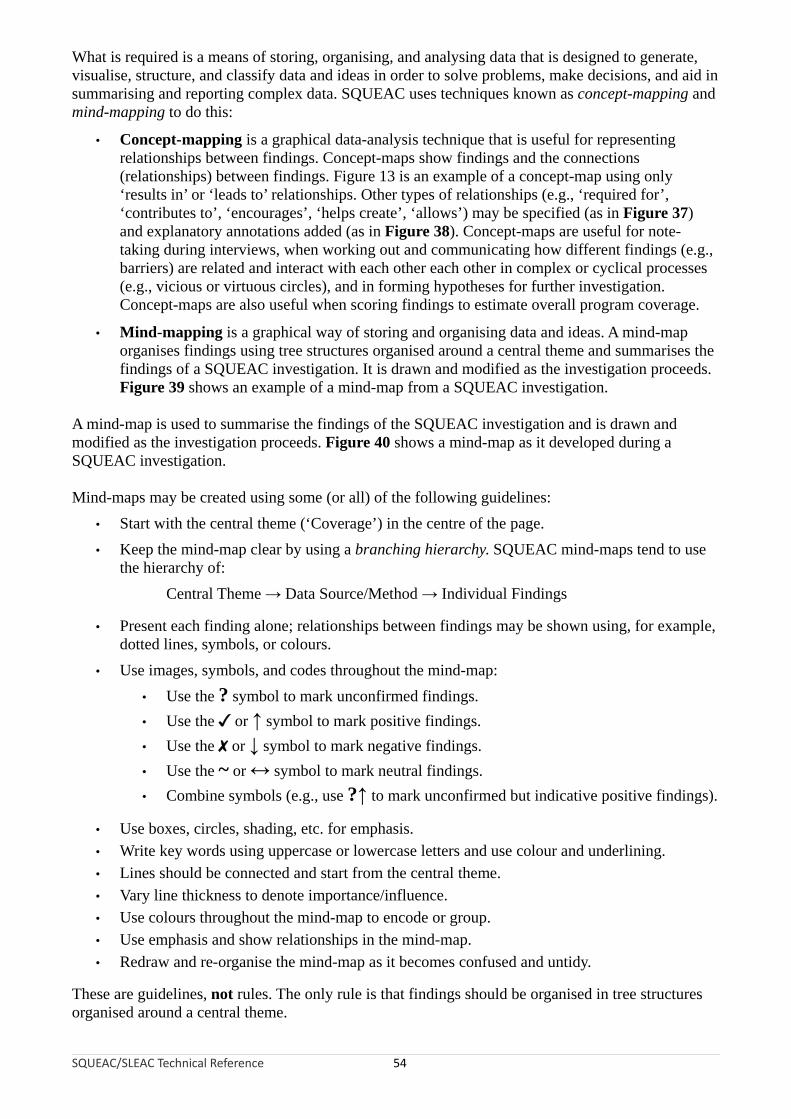
What is required is a means of storing, organising, and analysing data that is designed to generate, visualise, structure, and classify data and ideas in order to solve problems, make decisions, and aid in summarising and reporting complex data. SQUEAC uses techniques known as concept-mapping and mind-mapping to do this:

• Concept-mapping is a graphical data-analysis technique that is useful for representing relationships between findings. Concept-maps show findings and the connections (relationships) between findings. Figure 13 is an example of a concept-map using only ‘results in’ or ‘leads to’ relationships. Other types of relationships (e.g., ‘required for’, ‘contributes to’, ‘encourages’, ‘helps create’, ‘allows’) may be specified (as in Figure 37) and explanatory annotations added (as in Figure 38). Concept-maps are useful for note-taking during interviews, when working out and communicating how different findings (e.g., barriers) are related and interact with each other each other in complex or cyclical processes (e.g., vicious or virtuous circles), and in forming hypotheses for further investigation. Concept-maps are also useful when scoring findings to estimate overall program coverage.

• Mind-mapping is a graphical way of storing and organising data and ideas. A mind-map organises findings using tree structures organised around a central theme and summarises the findings of a SQUEAC investigation. It is drawn and modified as the investigation proceeds. Figure 39 shows an example of a mind-map from a SQUEAC investigation.

A mind-map is used to summarise the findings of the SQUEAC investigation and is drawn and modified as the investigation proceeds. Figure 40 shows a mind-map as it developed during a SQUEAC investigation.

Mind-maps may be created using some (or all) of the following guidelines:• Start with the central theme (‘Coverage’) in the centre of the page.• Keep the mind-map clear by using a branching hierarchy. SQUEAC mind-maps tend to use

the hierarchy of:Central Theme → Data Source/Method → Individual Findings

• Present each finding alone; relationships between findings may be shown using, for example, dotted lines, symbols, or colours.

• Use images, symbols, and codes throughout the mind-map:• Use the ? symbol to mark unconfirmed findings.• Use the ✓ or ↑ symbol to mark positive findings.• Use the ✗ or ↓ symbol to mark negative findings.• Use the ~ or ↔ symbol to mark neutral findings.• Combine symbols (e.g., use ?↑ to mark unconfirmed but indicative positive findings).

• Use boxes, circles, shading, etc. for emphasis.• Write key words using uppercase or lowercase letters and use colour and underlining.• Lines should be connected and start from the central theme.• Vary line thickness to denote importance/influence.• Use colours throughout the mind-map to encode or group.• Use emphasis and show relationships in the mind-map.• Redraw and re-organise the mind-map as it becomes confused and untidy.

These are guidelines, not rules. The only rule is that findings should be organised in tree structures organised around a central theme.


Figure 37. An example of a concept-map using explicitly defined relationship types


Note: This concept-map shows an example of a virtuous cycle driving coverage up and keeping coverage high.


Figure 38. An example of a concept-map using explicitly defined relationship types and an explanatory annotation

Data courtesy of UNICEF Sierra Leone, MOH Sierra Leone, and Valid International.

Note: This concept-map shows an example of a vicious cycle driving coverage down and keeping coverage low.


Figure 39. An example mind-map from a SQUEAC investigation

Original data courtesy of World Vision International

Coverage < 50%if > 5 km from site

CarerInterviews

Coveragequestions

Mismatch incase definition

Male permission?

Paths to treatment

Referral source

Active CBVs

Waiting time

Case-finding

Program sites

Stigma?

PHC

SFP

Community

Self

RoutineData

Monitoring

Default < 15%

Deaths < 5%

Cured < 80%

Admissions

Seasonality

Fits context?

Trend

Distance

Timely?

CBVInterviews

Motivation

Feel undervalued

TBAs and THPsinvolved?

Stigma?

CommunityIGDs

Stigma

Chief referrals

TBA referrals

THP referrals

Kwashiorkor?

Distance

No mobile clinics

Kwash.Study

Kwashiorkornot Included incase definition

SFPStudy

Weak interfacePoor monitoring

Small-AreaSurveys

SFP Interface

Coverage ≥ 50%if ≤ 5 km from site

ProgramCoverage

✘

✘

✘

✘

✘

✘

✘

✘

✘

✘

✔

✔

✔

✔

✔

✔

✘

✘

✘

✘

✔

✔

✔

✔

✔

✔

✔

✔

✔

✔

✔

✔

✔

✔

✔

108106

104102

10098

9694

9290

0

50

100

150

200

250

300

350

Admission MUAC

Treatment seeking


Figure 40. A mind-map being developed during a SQUEAC investigation

Photographs courtesy of World Vision International

Many people develop a personal style of mind-mapping. For example:

• The mind-map shown in Figure 39 uses symbols to mark positive (✓) and negative (✗) findings.

• The mind-map shown in Figure 40 and Figure 41 uses simple labels for findings; colours and labels to denote different data sources; symbols to denote positive, negative, and neutral findings; brackets and ‘clouds’ to group findings; and dashed lines to link findings from different data sources/methods.

These maps employ different styles to encode very similar information.


Figure 41. A completed SQUEAC mind-map (following from Figure 40)

Photograph courtesy of World Vision International

The style of mind-mapping extends to the organisation or branching hierarchy of the tree structure around the central theme. Trees may be organised using source → method → issue as branching hierarchy:


CentralTheme

Source

IssueMethod

Method

Method

Issue

Method

Findings

FindingsSource

Issue

Method Method

Issue

Method

Findings Findings

Source

Issue

Method

Method

MethodIssue

Method

Findings

Findings

or issue → source → method as the branching hierarchy:


CentralTheme

Issue

MethodSource

Source

Source

Method

Source

Findings

Findings

Issue

Method

Source Source

Method

Source

Findings Findings

Issue

Method

Source

Source

SourceMethod

Source

Findings

Findings

Other (or mixed) branching hierarchies may be used.

The branching hierarchy that is used may be suggested by the structure and progress of the SQUEAC investigation. Start by using the branching hierarchy that you are most comfortable with but be willing to redraw the mind-map using a different branching hierarchy should the original branching hierarchy prove awkward to use.

Mind-maps can be drawn by hand, using drawing software, or using mind-mapping software:

• Drawing mind-maps by hand is quick and simple and allows maps to be built collaboratively and encourages debate within the investigating team. Hand-drawn maps may also be used as ‘interactive exhibits’ in interviews. The untidy appearance (see, for example, Figure 41) emphasises the interim nature of findings during the early stages of an investigation.

• Drawing a mind-map on the computer using drawing software is useful for producing a fair copy of a hand-drawn mind map for inclusion in reports.

• Using mind-mapping software has many advantages:

• The mind-map can be restructured without having to redraw it from scratch.

• Mind-mapping software can also act as a sort of database with charts, spreadsheets, interview transcripts, interview summaries, concept-maps, etc. being stored ‘behind’ each node or leaf on the mind-map.

• The mind-map can easily be included in reports.

• Some mind-mapping software can use stored data to produce a report automatically.

Figure 42 shows a SQUEAC mind-map being edited using an open-source mind-mapping software package called XMind. This is available free from:

http://www.xmind.net/

This screenshot shows the text stored ‘behind’ the node for the findings of interviews with village doctors as well as a graph of routine program monitoring data. The XMind software can automatically produce a formatted and illustrated report using the entered findings and the hierarchical structure of the mind-map.

Most SQUEAC investigators use both hand-drawn mind-maps and mind-mapping software. It is particularly useful to use both methods during training. A large hand-drawn mind-map, such as is shown in Figure 40 and Figure 41, is useful for managing a SQUEAC investigation, providing a rich summary of the current state of the investigation and can serve as a focal point when deciding data-collection needs and dividing tasks between team members. The collaborative focus provided by the mind-map facilitates team building and improves the quality of the investigation.


Figure 42. A mind-map being edited using XMind



Combining and Confirming Findings from Routine Program and Qualitative Data

The data collected from routine program data and qualitative data, when combined, provide information about where coverage is likely to be satisfactory and where coverage is likely to be unsatisfactory, as well as information about the likely barriers to service access and uptake that exist within a program (Figure 36). This information can be considered or stated as a set of hypotheses that can be tested. The SQUEAC method uses small studies, small surveys, and small-area surveys to test these hypotheses.

Organising findings using concept-maps and mind-maps helps in formulating hypotheses. The findings shown in the mind-map in Figure 39, for example, suggested (amongst other things) the following hypotheses:

1. There will be a number of cases that were admitted to a supplementary feeding program (SFP) but that failed to respond and have become severely malnourished. This has not been recognised and they are now in the wrong program. These cases are not covered. This hypothesis was suggested by the absence of referrals from the SFP to the therapeutic feeding program (TFP). This hypothesis was tested by a small study at SFP sites, which revealed that there was no effective monitoring system in the SFP (leaving SAM cases undetected) and that SFP staff were unsure how to transfer cases from the SFP to the TFP. Small-area surveys also found SAM cases that were (inappropriately) in the SFP.

2. Distance between program sites and communities is a significant barrier to access. This is suggested by the analysis of admissions, by informal group discussions in outlying communities, and by the request for mobile clinics made in pastoralist communities. This hypothesis was tested using several small-area surveys undertaken in communities at different distances from program sites. These surveys found good coverage in communities located within 5 km of a program site and poor coverage in communities located further than 5 km from a program site.

Hypotheses about coverage should always be stated before undertaking small studies, small surveys, or small-area surveys. Hypotheses about coverage will usually take the form of identifying areas where the combined data suggest that coverage is likely to be satisfactory and areas where the combined data suggest that coverage is likely to be unsatisfactory. Figure 43, for example, shows an area of probable low coverage identified by mapping beneficiary home locations, analysis of outreach activities, defaulter follow-up, and qualitative data. The hypothesis about coverage in this area was:

• Coverage is below the Sphere minimum standard for coverage of TFPs in rural settings of 50% due to:

• A mismatch between the program’s definition of malnutrition (i.e., anthropometric criteria and problems of food-security) and the community’s definition of malnutrition (i.e., as a consequence of illness, particularly diarrhoea with fever).

• Patchy coverage of outreach services, particularly with regard to the ongoing follow-up of children with marginal anthropometric status.

• Distance to program sites and other opportunity costs.

A small-area survey was undertaken in this area to confirm this hypothesis. This survey involved using active and adaptive case-finding (see Box 3, page 65) in all villages in the area identified (shaded) in Figure 43 and the application of a questionnaire similar to that shown in Box 2 (page 49) to carers of non-covered cases found by the survey. Analysis of the collected data confirmed that coverage in the identified area was likely to be below 50%. The data are shown in Figure 44 and the details of the analysis are shown below.


Figure 43. Area of probable low coverage identified by mapping of home locations (shown), analysis of outreach activities, defaulter follow-up, and qualitative data

Photograph courtesy of Concern Worldwide


Box 3. Active and adaptive case-finding

The within-community case-finding method used in both SQUEAC small-area surveys, SQUEAC likelihood surveys, SLEAC, and CSAS surveys is active and adaptive:

Active. The method actively searches for cases rather than just expecting cases to be found in a sample.

Adaptive. The method uses information found during case-finding to inform and improve the search for cases.

Active and adaptive case-finding is sometimes called snowball sampling, optimally biased sampling, or chain-referral sampling.

The following method provides a useful starting point:

Ask community health workers, traditional birth attendants, traditional healers, or other key informants to take you to see ‘children that are sick, thin, have swollen legs or feet, or have recently been sick and have not recovered fully, or are attending a feeding program’ and then ask mothers and neighbours of confirmed cases to help you find more cases using existing cases as exemplars.

The basic case-finding question (i.e., ‘children that are sick, thin, have swollen legs or feet, or have recently been sick and have not recovered fully, or are attending a feeding program’) should be adapted to reflect community definitions/aetiologies of malnutrition and to use local terminology (e.g., using data collected in interviews such as those outlined in Box 1 (page 48), which will also help you choose appropriate key informants to assist you with case-finding). Markers of risk (e.g., orphans, twins, single parents, neglected or abused children, households without land or livestock) may also be included in the case-finding question. It is important to avoid, if possible, highly stigmatised terms (e.g., terms associated with poverty, child abuse or neglect, sexual libertinage, alcoholism) because community members may be reluctant to slander their neighbours to help you find SAM cases. It is important to ask about children attending a feeding program (or specific feeding programs). Failure to do this may result in bias toward low coverage in your surveys.

It is important that the case-finding method you use finds all or nearly all cases in the sampled communities. Formal evaluations of the type of active and adaptive case-finding described here have found that the method does find all or nearly all cases in the sampled communities provided that appropriate local terms and appropriate key informants are used. Interviews such as those outlined in Box 1 (page 48) are useful in designing the case-finding question and selecting the most useful key informants. Sampling stops only when you are sure that you have found all SAM cases in the community. Sampling in a community should not stop because you have reached a quota or met the sample size required by the survey. Such early stopping is not allowed.

Care needs to be exercised in the choice of key informant. Community leaders are a useful point of entry, but seldom make useful key informants. They are most useful in helping you find and recruit useful key informants. You should avoid relying solely on community health workers or volunteers that are attached to the program since they may be unable or reluctant to take you to see children that are not in the program.

It is important to realise that the active and adaptive case-finding method will fail in some settings. The method has been found not to work well in some refugee and IDP camp settings, in urban locations where there is a high population turnover (e.g., around railway and bus stations, newly established or growing peri-urban ‘shanties’), and in displaced and displacing populations. These settings are typified by a lack or loss of strong extra-familial relationships, extended familial relationships, strong local kinship ties, collective loyalty, and simple (traditional) social structures. In these settings, it may be very difficult to find useful key informants or local guides, and snowball sampling will not work well for finding SAM cases when people do not know their neighbours well. In these settings, it is also sensible to search for cases by moving house-to-house and door-to-door, making sure that you measure all children by taking a verbal household census before asking to measure children. This avoids sick or sleeping children being ‘hidden’ to avoid them being disturbed by the survey team.


Figure 44. Data from the small-area survey of the area shown in Figure 43


Program Site : Mwene-Ndeke

Note: Using the data presented in this table:

Point coverage:

Numerator = SAM cases in program= 3

Denominator = SAM cases= 12

Checking this against the 50% Sphere standard using simplified LQAS:

d =⌊ Denominator 12= = ⌊ 6 ⌋= 62 ⌋ ⌊ 2 ⌋

Since the numerator (3) is not greater than 6, the point coverage in the surveyed area is classified as being below 50%.

Period coverage:

Numerator = SAM cases in program + Recovering cases= 3 + 3= 6

Denominator = SAM cases in program + Recovering cases +SAM casesnot in program= 3 + 3 + 9= 15

Checking this against the 50% Sphere standard using simplified LQAS:

d =⌊ Denominator2 ⌋= ⌊ 15

2 ⌋= ⌊ 7.5 ⌋ = 7

Since the numerator (6) is not greater than 7, the period coverage in the surveyed area is classified as being below 50%.

Figure 45 shows the barriers to service access and uptake identified by analysis of questionnaire data from the small-area survey.


Figure 45. Barriers to service uptake found in a SQUEAC small-area survey








The findings of the small-area survey confirmed, in general terms, the hypothesis under test and also identified a problem with the application of case definitions leading to some cases being admitted to the wrong program (i.e., some SAM cases were admitted to the SFP due to confusion around the use of weight-for-height and MUAC in admission criteria).

Information collected regarding barriers to service access and uptake may also be used to inform the design of a questionnaire that is applied to carers of non-covered cases found by small-area surveys. A variation on the standard CSAS questionnaire, such as that shown in Box 2 (page 49), will usually be used for this purpose.

Small-area surveys are used to test hypotheses regarding the spatial distribution of coverage:• If previously collected data indicates that coverage is likely to be patchy then small-area

surveys are used to test this hypothesis. This requires surveys in areas where coverage is believed to be high as well as in areas where coverage is believed to be low.

• If previously collected data indicates that coverage is likely to be even then small-area surveys are used to test this hypothesis. The hypothesis states that coverage will be high (or low) wherever we look. This hypothesis can be tested by selecting survey areas at random. A better approach might be to select survey areas purposively (e.g., at different distances from program sites). A convenience sampling approach should never be used to test this hypothesis, as this is likely to sample areas close to program sites or along roads connecting program sites where coverage is expected to be similar.

Small-area surveys are used in almost all SQUEAC investigations.


Data Sources and Methods of Analysis

SQUEAC uses small studies and surveys to test hypotheses about coverage generated by the analysis of routine program data and qualitative data. Three types of investigation are commonly used:

Small studies. Small studies are usually short, semi-quantitative pieces of work that focus on testing a single hypothesis. The hypothesis being tested usually relates to processes that affects coverage rather than to coverage directly. Sampling and study design are directed by the hypothesis being tested. For example, testing a hypothesis that patient monitoring in an SFP was poor might be investigated by an observational study (i.e., a study in which the SFP processes are observed) at one or more SFP sites. If the hypothesis being tested can be expressed quantitatively (e.g., ‘less than 80% of cases that have been in the program for at least 4 weeks and have failed to gain weight have received counselling from clinic staff’) then data can be analysed using the simplified LQAS classification technique outlined below. Some small studies may be descriptive. In programs with high defaulting rates, for example, a small study finding defaulters and asking about reasons for non-attendance may provide information that can guide program reforms. Figure 46, for example, displays a ranked list of reasons for defaulting found in a rural CMAM program with unacceptably high levels of defaulting.

Small surveys. Small sample surveys are undertaken in population groups that are hypothesised to have high or low coverage (e.g., agrarians and pastoralists, Christians and Moslems). Each and every group is surveyed separately. If population groups live apart and members of each group are relatively easy to identify (e.g., agrarians and pastoralists) then separate small-area surveys (see below) in each population group may be undertaken. If population groups do not live apart then a single survey may be undertaken and data on group membership collected for all cases. The survey dataset may then be divided after data collection and the data from the different groups analysed separately. When using a single survey to collect data on two or more groups, you need to make sure that you use all appropriate local terms in case-finding questions. You may also need to recruit different key informants to help with case-finding in different groups. Data from small surveys may be analysed using the simplified LQAS classification technique outlined below.

Small-area surveys. Small-area surveys are small sample size surveys used to test hypotheses regarding the spatial distribution of coverage. Results may be combined with previously collected data (e.g., time-to-travel plots, carer interviews, half-distance between markets) to draw maps of coverage.

Small surveys and small-area surveys tend to use the same in-community sampling and data-collection methods as CSAS surveys, with communities or sub-communities selected purposively (i.e., directed by the hypothesis being tested). Cases are found using an active and adaptive case-finding method (Box 3, page 65). When a case is found, the carer is asked whether the child is already in the program. A short questionnaire (Box 2, page 49) is administered if the malnourished child is not already in the program.


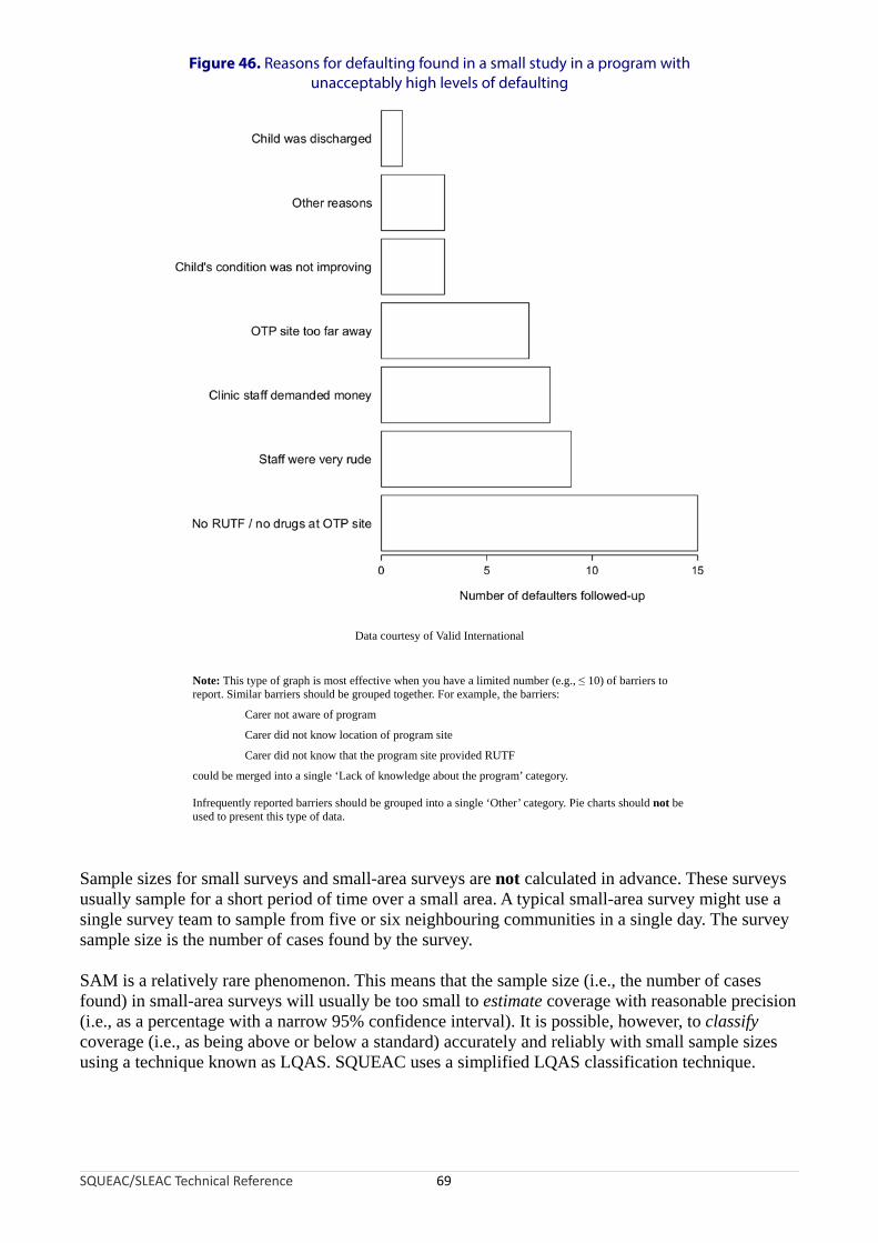
Figure 46. Reasons for defaulting found in a small study in a program with unacceptably high levels of defaulting

Data courtesy of Valid International







Sample sizes for small surveys and small-area surveys are not calculated in advance. These surveys usually sample for a short period of time over a small area. A typical small-area survey might use a single survey team to sample from five or six neighbouring communities in a single day. The survey sample size is the number of cases found by the survey.

SAM is a relatively rare phenomenon. This means that the sample size (i.e., the number of cases found) in small-area surveys will usually be too small to estimate coverage with reasonable precision (i.e., as a percentage with a narrow 95% confidence interval). It is possible, however, to classify coverage (i.e., as being above or below a standard) accurately and reliably with small sample sizes using a technique known as LQAS. SQUEAC uses a simplified LQAS classification technique.


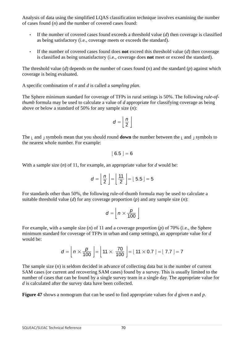
Analysis of data using the simplified LQAS classification technique involves examining the number of cases found (n) and the number of covered cases found:

• If the number of covered cases found exceeds a threshold value (d) then coverage is classified as being satisfactory (i.e., coverage meets or exceeds the standard).

• If the number of covered cases found does not exceed this threshold value (d) then coverage is classified as being unsatisfactory (i.e., coverage does not meet or exceed the standard).

The threshold value (d) depends on the number of cases found (n) and the standard (p) against which coverage is being evaluated.

A specific combination of n and d is called a sampling plan.

The Sphere minimum standard for coverage of TFPs in rural settings is 50%. The following rule-of-thumb formula may be used to calculate a value of d appropriate for classifying coverage as being above or below a standard of 50% for any sample size (n):

d = ⌊ n2 ⌋

The ⌊ and ⌋ symbols mean that you should round down the number between the ⌊ and ⌋ symbols to the nearest whole number. For example:

⌊ 6.5 ⌋ = 6

With a sample size (n) of 11, for example, an appropriate value for d would be:

⌊ n ⌋ ⌊ 11d = =

2 2 ⌋= ⌊ 5.5 ⌋ = 5

For standards other than 50%, the following rule-of-thumb formula may be used to calculate a suitable threshold value (d) for any coverage proportion (p) and any sample size (n):

d = ⌊ pn ×

100 ⌋For example, with a sample size (n) of 11 and a coverage proportion (p) of 70% (i.e., the Sphere minimum standard for coverage of TFPs in urban and camp settings), an appropriate value for d would be:

d = ⌊ pn ×

100 ⌋= ⌊ 7011 ×

100 ⌋= ⌊ 11 × 0.7 ⌋ = ⌊ 7.7 ⌋ = 7

The sample size (n) is seldom decided in advance of collecting data but is the number of current SAM cases (or current and recovering SAM cases) found by a survey. This is usually limited to the number of cases that can be found by a single survey team in a single day. The appropriate value for d is calculated after the survey data have been collected.

Figure 47 shows a nomogram that can be used to find appropriate values for d given n and p.


Figure 47. Simplified LQAS nomogram for finding d given n and p


0 5 10 15 20 25 30 35 40 450

10

20

30

40

50

d (round down to nearest whole number)

Sam

ple

size

(n

)p = 10% p = 20% p = 30% p = 40% p = 50% p = 60% p = 70% p = 80% p = 90%

Example showing d = 15 when n = 22 and p = 70%

Figure 44 shows the data collected in the small-area survey of the area shown in Figure 43. The survey found 12 current SAM cases and 3 of these cases were in the program. The appropriate value of d for a sample size (n) of 12 and a coverage standard of 50% is:

d = ⌊ n ⌋= ⌊ 12 = ⌊2 2 ⌋ 6 ⌋ = 6

Since 3 is not greater than 6, the coverage in the surveyed area is classified as being below 50% (i.e., coverage does not meet the 50% standard).

In a small-area survey undertaken in a rural CMAM program, nine current SAM cases were found and six of these cases were in the program. The appropriate value of d for a sample size (n) of 9 and a coverage standard of 50% is:

9d ⌊ n=

2 ⌋= ⌊ 2 ⌋= ⌊ 4.5 ⌋ = 4

Since 6 is greater than 4, the coverage in the surveyed area is classified as being greater than or equal to 50% (i.e., coverage meets or exceeds the 50% standard).

In a small-area survey undertaken in an urban CMAM program, nine current SAM cases were found and six of these cases were in the program. The appropriate value of d for a sample size (n) of nine and a coverage standard (p) of 70% (i.e., the Sphere minimum standard for coverage of TFPs in urban settings) is:

d = ⌊ pn ×

100 ⌋= ⌊ 709 ×

100 ⌋= ⌊ 9 × 0.7 ⌋ = ⌊ 6.3 ⌋ = 6

Since 6 is not greater than 6, the coverage in the survey area is classified as being below 70% (i.e., coverage does not meet the 70% standard).

If the hypothesis being tested in a small study can be expressed quantitatively then the simplified LQAS classification technique may be used to analyse the study data. For example, the study hypothesis is:

Less than 80% of cases that have been in the supplementary feeding program (SFP) for at least 4 weeks and have failed to gain weight have received counselling from clinic staff

Examination of 102 beneficiary record cards found 13 children that had been in the program for at least 4 weeks and had failed to gain weight. Short interviews with the carers of these children revealed that 4 of them had received counselling from SFP staff. The decision threshold is:

d = ⌊ pn × ⌋= ⌊ 80

13 × ⌋= ⌊ 13 × 0.8 ⌋ = ⌊ 10.4 ⌋ =10100 100

Since 4 is not greater than 10, the hypothesis is confirmed.

The simplified LQAS classification technique may be used to test whether the proportion of program beneficiaries requiring inpatient care at admission is not above a 5% standard. For example, an examination of beneficiary record cards for the 140 most recent program admissions found 5 cases requiring inpatient care:

d = ⌊ pn × ⌋= ⌊ 5

140 × 7100 ⌋= ⌊140 × 0.05⌋ =

100


Since 5 is not greater than 7, the proportion of program beneficiaries requiring inpatient care at admission is classified as being satisfactory (i.e., not above 5%).

The simplified LQAS classification technique may be used to classify the coverage of outreach activities. For example, using the data presented in Figure 23 and a coverage standard of 50% of villages in the program’s intended catchment area receiving five or more outreach visits in the previous 6 months:

d = ⌊ n2 ⌋= ⌊ 25

2 ⌋= ⌊ 12.5 ⌋ = 12

In this example, there are 25 villages in the program’s intended catchment area and 6 of them had received five or more outreach visits in the previous 6 months. Since 6 is not greater than 12, the coverage of outreach activities is classified as being unsatisfactory (i.e., below 50%). Note that the definition of success used here has both a spatial component (i.e., it is applied to each village separately) and a temporal component (i.e., frequency of five or more visits over a recent fixed period of the previous 6 months).

The simplified LQAS classification technique may also be used to classify defaulting and DNA rates. For example, using the data presented in Figure 34 and a standard for DNA rates of 15% (maximum):

d = ⌊ p 15n ×

100 ⌋= ⌊15 ×100 ⌋= ⌊ 15 × 0.15 ⌋ = ⌊ 2.25 ⌋ = 2

In this example, there are 7 DNA cases from 15 referrals. Since 7 is greater than 2, the DNA rate for referrals from this particular CBV is classified as being unsatisfactory (i.e., above 15%).

The results of all small studies, small surveys, and small-area surveys undertaken should be recorded on the investigation’s mind-map as results become available.

Using SQUEAC Data to Estimate Overall Program Coverage

The tools already presented in this section are capable of revealing a great deal about coverage and are sufficient to identify barriers to access and care and to devise appropriate remedial action. They do not, however, provide an overall estimate of program coverage. SQUEAC uses a Bayesian technique to provide this information when it is required.

In classical (frequentist) statistics, data collected using, for example, a survey are used to learn about unknown quantities, such as the coverage of a program. This is the approach used by the CSAS and SLEAC coverage survey methods. The classical approach uses only the survey data to estimate overall coverage. The survey data are treated as the only relevant source of information about coverage.

In Bayesian statistics, any relevant information may be used in addition to survey data. This is a useful approach for SQUEAC investigations because the analysis of routine program data; the intelligent collection of qualitative data; and the finding of small studies, small surveys, and small-area surveys can provide a great deal of relevant information about program coverage.

The main advantage to using the Bayesian approach is that smaller survey sample sizes are required. This is particularly useful when dealing with a rare condition, such as SAM. Another advantage of the Bayesian approach is that it provides a framework for thinking about SQUEAC data. The process of creating the prior (see below) has been found to be useful to SQUEAC investigators even when there was no intention of estimating overall coverage.


Bayesian methods allow findings from work done prior to a survey to be combined with data from the survey. Survey data are treated as just another source of information and are used to update the prior information:

Prior information Estimate of(SQUEAC tools) overall coverage

New information(SURVEY)

The prior information, survey data, and the resulting estimate have special names:

PRIOR POSTERIOR

LIKELIHOOD

The process of combining the prior and the likelihood to arrive at the posterior is known as a conjugate analysis. A conjugate analysis requires that the prior and the likelihood are expressed in similar ways.

The result of a survey may be viewed as a probability distribution. Figure 48, for example, shows the binomial probability density arising from a survey of 20 SAM cases of which 10 were covered:

• The point estimate (i.e., 50%) is the most likely value (mode) for coverage but other values, such as 35%, 42%, 48%, 58%, and 68%, are also probable values for coverage.

• Values for coverage below about 27% and above about 73% are not probable. These are the upper and lower 95% confidence limits for the point estimate.

• Values for coverage below about 18% and above about 82% are extremely unlikely.

The distribution of the likelihood in a Bayesian analysis of coverage will look something like the probability density shown in Figure 48.


Figure 48. Binomial probability density for coverage from a survey of 20 SAM cases of which 10 cases were covered

A conjugate analysis requires that the prior and the likelihood are expressed in similar ways. This means that the prior information about coverage (i.e., the findings from the analysis of routine programs data; the intelligent collection of qualitative data; and the finding of small studies, small surveys, and small-area surveys) must, like the likelihood, be expressed as a probability density.

The first step in expressing the prior information as a probability density is to make an informed guess about the most likely coverage value (the mode of the probability density) given the prior information. One way to do this is to use positive findings to ‘build up’ from zero (i.e., the lowest possible) coverage and to use negative findings to ‘knock down’ from 100% (i.e., highest possible) coverage.

Figure 49 shows the prior information from a SQUEAC investigation grouped into positive and negative findings.


Positive Findings Negative Findings

Finding

Scores

Finding

Scores

Simple Weighted Simple Weighted

Self-referrals 5% 5% Poor interface with SFP 5% 5%

Referrals from the community:

Carers of previous patients

Village leaders

Traditional healers

TBAs

5% 5%Lack of formal involvement of traditional healers and TBAs for case-finding and referral

5% 5%

Timely treatment seeking (admission MUAC) 5% 5% Poor remuneration of CBVs 5% 3%

Program indicators:

High proportion cured

Low mortality

Low defaulting

5% 5% Lack of oedema a sign in program messages and training of CBVs 5% 3%

Reduction of stigma associated with malnutrition 5% 3% Declining trends in admissions 5% 3%

Active cadre of CBVs 5% 3% SUM OF SCORES 25% 19%

Spatial homogeneity (small-area surveys) 5% 3%

Coverage questions (from carer interviews) 5% 1%

Short waiting times/efficient patient flow at program sites 5% 1%

Admissions respond by season 5% 1%

SUM OF SCORES 50% 32%


Figure 49. Prior information from a SQUEAC investigation grouped into positive and negative findings with simple and weighted scores


The simplest approach to deciding the mode of the prior is to score all findings equally (labelled ‘Simple’ in Figure 49, which uses a score of 5 for all findings). The positive scores are added together. The sum of the negative scores is subtracted from 100%. The average of the two resulting numbers is then taken. Using the ‘Simple’ scores presented in Figure 49:

50 % + (100% − 25%) 50 % + 75 %Prior Mode = = = 62.5%

2 2

Another approach to deciding the mode of the prior is to use scores or weights that reflect the relative importance or likely effect on coverage of each finding (labelled ‘Weighted’ in Figure 49, which uses scores between 1 and 5 to denote importance or the likely effect of each finding). The positive scores are added together. The sum of the negative scores is subtracted from 100%. The average of the two resulting numbers is then taken. Using the ‘Weighted’ scores presented in Figure 49:

32% +(100% − 19%) 32 % + 81 %Prior Mode = = = 56.5%

2 2

The ‘Weighted’ approach requires a more thorough review of the prior information than the simpler method. The principal advantage of this approach is that it is likely to yield a more credible value for the mode of the prior than the simpler method. This approach does not involve any extra work, because ranking of findings by their relative importance is something that will need to be done for reporting purposes.

It should be noted that these methods can produce silly results (i.e., prior modes below 0% or above 100%). For example, with an investigation with 24 positive results and 3 negative results all receiving a score of 5, this method would give an impossible value for the prior mode of:

120% +(100% − 15%) 120% + 85%Prior Mode = = = 102.5%

2 2

In cases such as this, the maximum score could be scaled so that neither the sum of positive scores or the sum of negative scores can exceed 100%. In the example given above a suitable maximum score might be:

Maximum score = ⌊10024 ⌋= 4

Using a maximum score of 4 gives:

96 % + (100% − 12 %) 96 %+ 88 %Prior Mode = = = 92%

2 2

Figure 50 presents an alternative approach to deciding the mode of the prior using estimates of program performance for key processes associated with coverage (i.e., recruitment, treatment seeking, defaulting).

These methods can yield a first guess at a credible value for the mode of the prior and should be reviewed by returning to the prior information and, if necessary, recalculated or adjusted. The value of the mode of the prior may be changed at any time before you start collecting data for the likelihood survey. If data from previous CSAS surveys, SLEAC surveys, or SQUEAC investigations are available then they may also be used to help decide a credible value for the mode of the prior.


Figure 50. Deciding the mode of the prior as the product of program performance at key processes associated with program coverage



There is always uncertainty about the value of the prior mode. The amount of uncertainty about the mode of the prior is the same as the probable range of values of coverage that is consistent with the prior information. This is specified using:

• The minimum probable value for coverage that is consistent with the prior information

• The maximum probable value for coverage that is consistent with the prior information

A simple way of doing this is to use a fixed quantity, such as ± 25 percentage points. For example, with the prior information summarised in Figure 49, a value of 56.5% for the prior mode was decided. A suitable minimum probable value for this prior might be:

Minimum probablevalue = 56.5% − 25% = 31.5%

A suitable maximum probable value for this prior might be:

Maximum probable value = 56.5% + 25% = 81.5%

If there is very little uncertainty about the value of the prior mode then ± 20 percentage points might be used. It is seldom appropriate (and particularly in a program’s first SQUEAC investigation) to use a smaller value than ± 20 percentage points when specifying uncertainty about the prior mode.

There is no requirement that the distribution of the prior be symmetrical about its mode. If, for example, the maximum probable value of 81.5% calculated above is considered to be extremely unlikely (i.e., it is considered extremely unlikely that coverage could be as high as 81.5%) then it could be replaced with a more credible value (e.g., 75%).

Another situation when a symmetrical prior is likely to be unsuitable is when coverage is expected to be either very low or very high. If, for example, coverage is expected to be about 20% then values for the minimum and maximum probable values of 10% and 40% might be specified.

Note that coverage cannot be below 0% or above 100%. This means that the minimum probable value cannot be below 0% and the maximum probable value cannot be above 100%.

Another way of deciding minimum and maximum probable values is to draw a histogram prior:1. Draw x and y axes. Label the x axis ‘Coverage’ and mark a scale of 0% to 100% in 10%

intervals (decades). Label the y axis ‘Probability’ or ‘Belief’.2. Mark the prior mode with a tall column.3. Mark the extremely unlikely values with horizontal lines close to the x axis.4. Mark the relative (i.e., to the prior mode) probability of coverage for each remaining decade.5. Draw a smooth line that captures the shape of the histogram.6. Mark the position of the minimum and maximum probable values.

This process is illustrated in Figure 51. In this example, the prior mode is about 55% and the minimum and maximum probable values are about 25% and 80%, respectively.

When deciding suitable values to describe the prior, it is important to be realistic about the strength of the prior information. The use of a narrow range of probable values should only be used when there is very little uncertainty about coverage. The mode and the minimum and maximum probable values of the prior distribution should be credible and reflect the prior information, not wishful thinking.


Figure 51. Steps in drawing a histogram prior


Drawx-y axes

Markprior mode

Mark decadeson x axis

Draw a smoothline to representthe prior density

Minimumprobable

value

Maximumprobable

value

Mark extremelyunlikely values

Mark probabilityfor each coverage

decade

Continue tomark probability

for each coveragedecade


The conjugate analysis method used in SQUEAC requires the distribution of the prior to be summarised by two numbers called shape parameters, which are labelled αPrior and βPrior. Suitable values for αPrior and βPrior may be calculated using the mode and the minimum probable value and maximum probable value of the prior with the following formulas:

minimum + 4 × mode + maximumμ =6

maximum − minimumσ =6

αPrior = μ ×(μ × (1 − μ)σ2 − 1)

(μ × (1 − μ)βPrior =(1 −μ) ×

σ 2 − 1)It should be noted that these formulas require values to be expressed as proportions, not percentages.

To convert a percentage to a proportion:

PercentageProportion =

100

For example, 55% expressed as a proportion is:

55 = 0.55100

Applying the formulas for calculating αPrior and βPrior to a prior with a mode of 55% and the minimum and maximum probable values of 25% and 80% (from Figure 51) yields:

0.25 + 4 × 0.55 + 0.80μ = = 0.546

0.80 − 0.25σ = = 0.096

0.54 × (1 − 0.54)αPrior = 0.54 × ( − 1

0.0081 )= 16.02

βPrior =(1 − 0.54)× (0.54 ×(1 − 0.54)−1)= 13.65

0.0081

A prior distribution created using these αPrior and βPrior is shown in Figure 52. Note how similar this is to the prior distribution in the histogram prior (Figure 51).


25% 55% 80%

Figure 52. The Beta(16.02, 13.65) prior

The formulas for calculating αPrior and βPrior given above provide approximate values. The approximate values produced by these formulas are, however, accurate enough for practical purposes.

Table 4 shows approximate values for αPrior and βPrior for different prior modes at two different levels of uncertainty (i.e., ± 25 percentage points and ± 20 percentage points) calculated using these formulas. The values given in Table 4 are likely to be useful in the majority of SQUEAC investigations.

When deciding a suitable range for the prior, it is important to be realistic about the strength of the prior information. In SQUEAC investigations, values of αPrior and βPrior above 35 are likely to be inappropriately high. Values of αPrior and βPrior that are much above 35 should be used only when you are very certain about the true value of program coverage and will usually only be appropriate after a series of SQUEAC investigations or if coverage has been been estimated by a reasonably recent CSAS survey or classified by a reasonably recent SLEAC survey.


Table 4. Approximate values for αPrior and βPrior for different prior modes at two different levels of uncertainty


Uncertainty

± 25 percentage points ± 20 percentage points

Prior mode αPrior βPrior αPrior βPrior

20% 7.0 28.0

25% 6.5 19.5 10.3 30.9

30% 8.8 20.5 13.9 32.4

35% 11.1 20.6 17.6 32.6

40% 13.4 20.1 21.2 31.8

45% 15.6 19.1 24.6 30.1

50% 17.5 17.5 27.6 27.6

55% 19.1 15.6 30.1 24.6

60% 20.1 13.4 31.8 21.2

65% 20.6 11.1 32.6 17.6

70% 20.5 8.8 32.4 13.9

75% 19.5 6.5 30.9 10.3

80% 28.0 7.0

Example of use

Prior mode : 55%Uncertainty : ± 25%

αPrior : 19.1From table

βPrior : 15.6

The values given in the table are approximate but are accurateenough for practical purposes.

Prior information expressed using the αPrior and βPrior shape parameters can be combined with survey (likelihood) data using a conjugate analysis:

Conjugateanalysis

PRIOR POSTERIOR

LIKELIHOOD

Survey (likelihood) data can be summarised using a numerator and a denominator. For example, the formula for a simple (point) coverage estimator is:


Coverage = Number of current cases attending the programNumber of current cases

Numerator

Denominator

A conjugate analysis combines the αPrior and βPrior shape parameters for the prior with the numerator and denominator of the likelihood survey estimator to give the posterior probability density:

Conjugateanalysis

PRIOR POSTERIORBeta(α

Prior , β

Prior) Beta(α

Prior+ numerator, β

Prior+ denominator - numerator)

LIKELIHOODBinomial(denominator, numerator)

The posterior probability density is:

Posterior = Beta prior numerator, prior denominator − numerator

The terms:

prior numerator and priordenominator − numerator

in the formula used to calculate the posterior are the αPosterior and βPosterior shape parameters for the posterior.

The αPosterior and βPosterior shape parameters may be used to find the mode of the posterior:

αmode = Posterior − 1

αPosterior + βPosterior − 2

The mode of the posterior is the estimate of program coverage.

An approximate 95% credible interval (i.e., the Bayesian equivalent of a 95% confidence interval) on the mode of the posterior may be calculated using the following formula:

α ×β95% CI = mode ± 1.96 ×√ Posterior Posterior

(α 2Posterior + βPosterior ) × (αPosterior + βposterior + 1)

These formulas return values expressed as proportions rather than as percentages. To convert a proportion to a percentage:

Percentage =Proportion × 100

For example, 0.55 expressed as a percentage is:

0.55 × 100 = 55%

The formula for calculating the 95% credible interval returns reasonably accurate results when the values of the αPosterior and βPosterior shape parameters are both greater than or equal to 10 and:

αPosterior +βPosterior − 2 ≥ 30

The formula for calculating the 95% credible interval may return inaccurate results when either of the αPosterior and βPosterior shape parameters have a value below 6 and the posterior mode is very different from 50%.

An Example Conjugate Analysis

Evaluation of the prior information in a SQUEAC assessment led to the selection of a prior with the distribution Beta(34, 27). The likelihood survey found 24 SAM cases (the denominator) of which 9 (the numerator) were covered.

The resulting posterior is:

Posterior = Beta 34 9, 27 24 − 9 = Beta 43,42

The values 43 and 42 are the αPosterior and βPosterior shape parameters for the posterior.

The estimate of program coverage is:

43 − 1 42mode = = = 0.506 (50.6%)

43 + 42 − 2 83


The αPosterior and βPosterior shape parameters are both greater than or equal to 10 and:

αPosterior +βPosterior − 2 = 83 (which is ≥ 30)

So we can calculate an approximate 95% credible interval for this estimate:

×95%CI 0.506 ± 1.96 ×√ 43 42= 2 = {0.400, 0.612 } = { 40.0% , 61.2%}(43 + 42) × (43 + 42 + 1)

This example conjugate analysis may be summarised as:


PRIORDistribution = Beta(34, 27)

Mode = 56.0% (95% CI ≈ 43.6%; 68.4%)

LIKELIHOODDistribution = Binomial(24, 9)

Mode = 37.5% (95% CI = 18.8%; 59.4%)

POSTERIORDistribution = Beta(43, 42)

Mode = 50.6% (95% CI ≈ 40.0%; 61.2%)

Conjugateanalysis

and is plotted in Figure 53.

The conjugate analysis combines a beta distributed prior with a binomial distributed likelihood to produce a beta distributed posterior:

Conjugateanalysis

PRIOR POSTERIORBeta(α

Prior , β

Prior) Beta(α

Prior+ numerator, β

Prior+ denominator - numerator)

LIKELIHOODBinomial(denominator, numerator)

This procedure is known as a beta-binomial conjugate analysis.

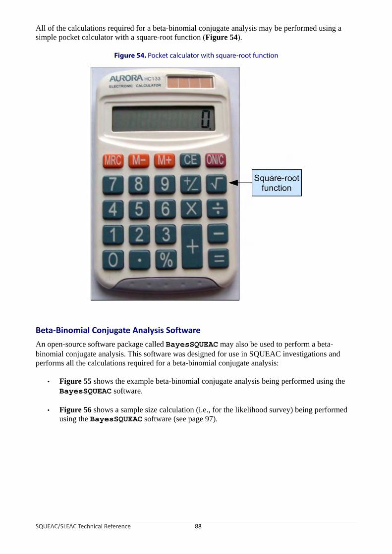
All of the calculations required for a beta-binomial conjugate analysis may be performed using a simple pocket calculator with a square-root function (Figure 54).

Figure 54. Pocket calculator with square-root function

Beta-Binomial Conjugate Analysis Software

An open-source software package called BayesSQUEAC may also be used to perform a beta-binomial conjugate analysis. This software was designed for use in SQUEAC investigations and performs all the calculations required for a beta-binomial conjugate analysis:

• Figure 55 shows the example beta-binomial conjugate analysis being performed using the BayesSQUEAC software.

• Figure 56 shows a sample size calculation (i.e., for the likelihood survey) being performed using the BayesSQUEAC software (see page 97).


Figure 55. The example beta-binomial conjugate analysis using BayesSQUEAC


Figure 56. Using BayesSQUEAC to calculate the sample size required to estimate coverage with a precision of ± 10% using a Beta(29, 13) prior using the simulation approach

Different numerators and denominators are tried until the displayed estimate shows the required precision

The BayesSQUEAC software also simplifies the process of performing a beta-binomial conjugate analysis by:

• Allowing the specification of the prior as a curve that matches the shape of a histogram prior without the need to calculate the αPrior and βPrior shape parameters.

• Automatic calculation of the posterior mode and 95% credible interval.

• Production of summary/diagnostic plots of the beta-binomial conjugate analysis.

• Allowing calculation of the likelihood sample size by simulation.

The BayesSQUEAC software is available for free from:

http://www.brixtonhealth.com/bayessqueac.html


Diagnosing Coverage Estimates

It is important to realise that the beta-binomial conjugate analysis method used in SQUEAC has an important limitation. If the sample size used for the likelihood survey is small and the prior is both inaccurate and strong then the prior will dominate the analysis and the resulting coverage estimate will be biased (i.e., inaccurate). An inaccurate prior is one in which the mode of the prior is very different from the the true coverage proportion. The tendency is for the prior to overestimate coverage. This mistake is common when investigating the coverage of your own programs. It is also commonly made by inexperienced SQUEAC investigators who tend to favour evidence from program staff over other evidence from other sources. A strong prior is one with a narrow range of probable values and large values of the αPrior and βPrior shape parameters. The use of a narrow range of probable values should only be used when there is very little uncertainty about coverage and is almost never appropriate in the first SQUEAC investigation of a program.

The sample size that can be collected for the likelihood survey is limited by prevalence and the time and resources available. This means that the only way to avoid this bias problem is to be scrupulous when specifying the prior. This means being realistic about the position of the prior mode and realistic about how much the prior information can tell you about coverage. If you are unsure about the position of the prior mode then you should specify a weak prior with a wide range of probable values by using small values for the αPrior and βPrior shape parameters.

You will only know if you have specified a prior that is both inaccurate and strong after you have analysed the data. If you find that coverage estimated from the likelihood data alone using:

NumeratorCoverageLikelihood = × 100

Denominator

is very different from the position of the prior mode then the prior and the likelihood are said to conflict and the results of the beta-binomial conjugate analysis should be treated with caution.

The BayesSQUEAC software automatically produces a summary/diagnostic plot of the beta-binomial conjugate analysis. If there is little or no overlap between the distributions of the prior and the likelihood then the prior and likelihood conflict (see Figure 57). Note that the posterior is of similar width to the prior when the prior and the likelihood conflict. This means that the likelihood survey has not reduced uncertainty about coverage (i.e., it was a waste of time and resources).

There is nothing that you can do to fix the problem if the prior and the likelihood conflict other than report the problem or start the survey from scratch with a more realistic prior and collect new data. It is better, therefore, to avoid the problem by being scrupulous when specifying the prior.


Figure 57. Illustration of the effect of the strength and accuracy of three different priors on the posterior coverage estimate in a population with true coverage of 28% with identical likelihoods


Likelihood Surveys: Sampling and Sample Size

The likelihood survey will usually use a two-stage sampling procedure:

First stage sampling method. This is the sampling method that is used to select the villages to be sampled. CSAS assessments use the centric systematic area sampling or quadrat method to select villages to be sampled. A similar method could be used to select villages to be sampled for the SQUEAC likelihood survey. The number of quadrats drawn on the map may be much smaller than would be used for a CSAS assessment (this is the same as using larger quadrats). The villages to be sampled may be selected by their proximity to the centre of each quadrat, as is done in a standard CSAS survey (Figure 58 and Figure 59). The number and size of quadrats should be selected so as to spread the sample of villages over the entire program area. Many small quadrats are better than few large quadrats. For example, the sample illustrated is Figure 59 (19 quadrats) spreads the sample more evenly and over more of the program catchment area than the sample illustrated in Figure 58 (8 quadrats). You should use as many quadrats as is feasible with the time and resources available for the survey. The CSAS/quadrat sampling method is appropriate for estimating coverage over a wide area such as a health district. Another useful approach is to stratify by clinic catchment area and select villages systematically from a complete list of villages sorted by clinic catchment area (Figure 60). This approach may be used with any areas (e.g., administrative areas) for which complete lists of villages are available. The first stage sampling method should be a spatial sampling method that yields a reasonably even spatial sample from the entire program catchment area. Cluster sampling using population proportional sampling (PPS), such as that used for Standardised Monitoring and Assessment of Relief and Transition (SMART) surveys, is not appropriate. The stratified approach outlined above and illustrated in Figure 60 provides a reasonably even spatial sample using village lists and does not require the use of maps. It is important to note that sampling should not stop when the survey has reached its required sample size. Sampling stops only after you have sampled all of the selected villages.

A within-community sampling method. This will usually be an active and adaptive case-finding method or a house-to-house census sampling method (see Box 3, page 65). These methods find all, or nearly all, current and recovering SAM cases in a sampled village. Sampling should be exhaustive. This means that you stop sampling only when you are sure that you have found all cases in the community. Sampling should not stop when you have met a quota or when the wider survey has reached its required sample size.

This is a two-stage sample because a sample of villages in the program catchment area is taken first (Stage 1) and then a ‘census’ sample of current and recovering SAM cases is taken from each and every one of the selected villages (Stage 2). The likelihood survey is a wide-area survey of the entire program catchment area.

The CSAS/quadrat approach is useful for a single survey. If you repeat the survey then the same villages will be sampled. This may cause the survey to overestimate coverage because we expect coverage to have been improved by case-finding and referral in the sampled villages. One way around this problem is to sample villages at random from each quadrat. This will yield independent samples at each survey round. Do not exclude previously sampled villages. This may cause the survey to underestimate coverage and you will eventually run out of villages to sample.


Figure 58. A coarse CSAS/quadrat sample of villages

Intended catchment

Major road

Towns and villages

Sampling locations

Legend


Figure 59. A finer and wider CSAS/quadrat sample of villages than in Figure 58

Intended catchment

Major road

Towns and villages

Sampling locations

Legend


Figure 60. Villages selected using stratified systematic sampling

Intended catchment

Major road

Towns and villages

Sampling locations

Legend

Clinic catchment

Program site

Sampling locations (villages) were selected systematically from a complete list of villages sorted by cliniccatchment area. This method can be performed using village lists and does not require a map.

Note that the sample is reasonably evenly spread over the entire survey area.


The sample size required for a likelihood survey depends on the prior and the precision required for the posterior estimate and can be calculated using the following formula:

mode ×(1 −mode )nLikelihood =⌈ (precision ÷ 1.96)2

− (αPrior +βPrior − 2)⌉where mode is the mode of the prior, αPrior and βPrior are the shape parameters of the prior, and precision is the precision required for the posterior estimate.

The ⌈ and ⌉ symbols mean that you should round up the number between the ⌈ and ⌉ symbols to the nearest whole number. For example:

⌈ 24.5 ⌉ = 25

It should be noted that this formula requires mode and precision values to be expressed as proportions, not percentages.

For example, estimating coverage with a precision of ± 10% using a Beta(29, 13) prior with a mode of 70% would require a likelihood survey with a sample size:

0.7 ×(1 − 0.7)nLikelihood =⌈ 29

( ÷ 1.96)2−( + 13 − 2)

0.1 ⌉= 41

Sample sizes for likelihood surveys are usually calculated to achieve a precision of ± 10 percentage points or better on the posterior estimate. This is the same precision as provided by the Expanded Program of Immunisation (EPI) vaccine coverage survey method. It is common practice to specify broader precisions (e.g., ± 15 percentage points or even ± 20 percentage points) and use smaller sample sizes when populations are sparse or small and the prevalence of SAM is low. In these contexts, it will be very difficult to collect a large sample and the sample size of the likelihood survey will be decided by what can be collected with the time and resources available for the survey.

The precision of the posterior estimate can be improved by increasing the sample size of the likelihood survey or by using a stronger prior (i.e., a prior with larger αPrior and βPrior shape parameters). It is only legitimate to use a stronger prior if you collect more data that allows you to specify a stronger prior. It is never legitimate to use a stronger prior to increase precision of the posterior estimate without collecting more data.

It is a good idea to use a minimum sample size of about:

nmin = αPrior + βPrior − 2

Using the example above:

nmin = αPrior +βPrior − 2

nmin = 29 + 13 − 2 = 40

Since 40 is less than or equal to 41, it would be safe, in this example, to use n = 41 in the likelihood survey.


The purpose of this minimum sample size guideline is to ensure that the sample size of the likelihood survey is sufficiently large to be able to correct a poorly specified prior. Since a prior defined as Beta(αPrior, βPrior) is equivalent to a survey with a sample size of:

n = αPrior + βPrior − 2

the formula for nmin:


ensures that the likelihood is at least as strong as the prior.

It is important to apply the minimum sample size guideline when there is considerable uncertainty about the accuracy of the prior (which should also be reflected in small values of αPrior and βPrior shape parameters of the prior).

If you are using a prior with small values of αPrior and βPrior and will be analysing data by hand using the formulas presented above then you should check that your survey sample size is likely to result in values of αPosterior and βPosterior that are greater than or equal to 10:

⌊ αPrior + mode × nLikelihood ⌋ ≥ 10 and ⌊ βprior + nLikelihood − mode × nLikelihood ⌋≥ 10

You should also check that:

αPrior + βprior + nLikelihood − 2 ≥ 30

If, for example, you are using a Beta(5, 7) prior that has a mode of 40% then a sample size of at least n = 20 is required since:

⌊ 5 + 0.4 × 20 ⌋ = 13 and ⌊ 7 + 20 − 0.4 × 20 ⌋ = 19 and 5 + 7 + 20 − 2 = 30

The purpose of this minimum sample size guideline is to ensure that the formula for calculating the 95% credible interval returns reasonably accurate results.

BayesSQUEAC can be used to calculate sample sizes using a simulation approach:

• The prior is specified using the ‘Prior α’ and ‘Prior β’ sliders.

• The expected survey data (i.e., different numerators and denominators) are simulated so that:

numerator ≈ demominator × prior mode

A convenient way of doing this is to change the sample size using the ‘Denominator’ slider and then change the numerator using the ‘Numerator’ slider so that the modes of the prior and the likelihood coincide. This is usually much quicker than calculating the numerator for each change in the denominator.

• Different numerators and denominators are tried systematically until the displayed estimate shows the required precision. The denominator at this point is the required sample size.

Figure 56 shows BayesSQUEAC being used to calculate a sample size to estimate coverage with a precision of ± 10% using a Beta(29, 13) prior with a mode of 70%.


A similar approach may be used to find a minimum sample size. Different numerators and denominators are tried systematically until the likelihood has the same mode and the same strength and width as the prior, as is the case in Figure 56.

The calculated sample size is the number of SAM cases (n) required. This needs to be translated into the minimum number of villages that need to be sampled to achieve this sample size. This is done using the following formula:

nvillages = ⌈ npercentage of population

average village population 6 – 59 months SAM prevalenceall ages × ×

100 100 ⌉The percentage of children aged between 6 and 59 months is usually assumed to be about 20% in developing countries. You should use 20% unless you have better information from, for example, a recent census or population survey or Demographic and Health Survey (DHS).

SAM prevalence refers to the average SAM prevalence in the program catchment area. It is unlikely that this will be known or known with good precision. SAM prevalence estimates may be available from previous nutritional anthropometry surveys (e.g., SMART surveys). SAM prevalence varies throughout the year (e.g., prevalence is usually higher before harvests than after harvests). This means that you should use the results from a nutritional anthropometry survey undertaken at the same time of year as the current SQUEAC assessment.

It is better to use a low rather than a high estimate of SAM prevalence for this sample size calculation. A value midway between the point estimate and the lower 95% confidence limit for SAM prevalence could be used. For example, if the prevalence of SAM is estimated as 1.2% (95% CI = 0.6% – 2.6%) then a suitable low estimate would be:

1.2 − 0.6Prevalence = 1.2 − = 0.9%

2

Using a low estimate helps ensure that the survey will achieve the target sample size.

Note that prevalence here is the estimated prevalence of the program’s admitting case definition. This will usually not be the weight-for-height based ‘headline’ prevalence estimate reported by a SMART survey. The required estimate will usually be found in the needs assessment section of a SMART survey report.

If you do not have nutritional anthropometry survey results from the same time of year as the current SQUEAC assessment then you should use results from the most recent nutritional anthropometry survey and adjust them using, for example, seasonal calendars of human disease (Figure 6, Figure 11, and Figure 12), calendars of food availability (Figure 6, Figure 11, and Figure 12), agricultural calendars (Figure 6, Figure 11, and Figure 19), long-term admissions data from nutrition programs (Figure 8), and long-term returns from growth monitoring programs.

The formula for the calculation of the minimum number of villages that need to be sampled to achieve the required sample size shown above assumes that the case-finding method being used will find all, or nearly all, current and recovering SAM cases in sampled villages. If you are unsure of this then you should sample a larger number of villages.

You should monitor the number of cases that are found during the likelihood survey and be prepared to increase the number of villages that will be sampled if many fewer cases than expected are being found.


SQUEAC Survey Sample Size Example

Here is an example of the required sample size calculations:

Target sample size. A target sample size (n) of 41 cases was calculated using a Beta(29, 13) prior and a desired precision of ± 10%:

n = ⌈ 0.7 × (1 − 0.7)− (29 + 13− 2) = 41

(0.1 ÷ 1.96)2 ⌉Number of villages to be sampled. The following information was used to calculate the number of villages to be sampled:

Target sample size : 41Average village population (all ages) : 600

Prevalence of SAM : 1%Percentage of children aged between 6 and 59 months : 20%

Using this information, the minimum number of villages to be sampled was calculated to be:

nvillages = ⌈ 41 =20 1 35600 × ×100 100 ⌉

When area sampling is used (see Figure 58 and Figure 59) then the villages to be sampled are distributed evenly between the areas. For example, if a CSAS/quadrat sample with eight quadrats, such as that shown in Figure 58, is used and at least 35 villages are to be sampled then:

⌈ 35 ⌉= ⌈4.38⌉ = 58

villages will need to be sampled from each quadrat.

If a CSAS/quadrat sample with 19 quadrats, such as that shown in Figure 58, is used and at least 35 villages are to be sampled then:

⌈ 3519 ⌉= ⌈1.84 ⌉ = 2


If a first stage sample such as that shown in Figure 60 is used then 35 villages need to be sampled systematically from a complete list of villages sorted by stratum.

In the case of a CSAS sample (e.g., Figure 58 and Figure 59), villages to be sampled are selected by their proximity to the centre of each quadrat (Figure 61). This selects clusters of villages and reduces the travel time between villages selected to be sampled. This allows more villages to be sampled by a survey team in a day.


Figure 61. Selection of villages to be sampled using CSAS sampling

Quadratboundary

Villagenot selected

Selected villages (5)

Centre of quadrat

×××

×

×

×××

××

×

××

×

×

A CSAS sample requires a map. If a map is not available then an alternative spatial stratification method may be used. Figure 60 shows a sample stratified by clinic catchment area. Any areal unit or subdivision for which complete lists of villages are available (e.g., counties, vice-counties, chiefdoms, electoral divisions) may be used. Figure 62, for example, illustrates the process of taking a spatially stratified systematic sample from a list of villages sorted by chiefdom. This type of sample also spreads the sample over the entire survey area.

Box 2 (page 49) shows an example of a simple structured interview questionnaire that may be applied to carers of non-covered cases found during likelihood surveys. The questionnaire shown in Box 2 yields qualitative data (i.e., questions regarding the how? and why? of decision making in carers of non-covered cases) that can be analysed using simple quantitative techniques as in Figure 2 and Figure 45.


Figure 62. Selection of villages to be sampled using spatially stratified sampling


1

2

3

4

5

6

7

8

9

10

11

12

13

14

15

16

17

18

19

20

21

22

23

24

Benguema

Fabaina

Koya

Gbendembu

Songo

Madonkeh

Urugli

Bottomupi

Redpu

Borioboolagah

Portei

Tombo

Ashu

Foulah

Juba-Kaningo

Sattia

Kissykissy

Low Cost Housing

Magbafti

Adonkia

Pamaronku

Fourah

Kokupa

Jalloh

Kuntola

Mayankeni

Kroo

Chiefdom Village Number

Villages sorted by chiefdom(stratification is by chiefdom)

We need a random startingpoint between one and the

sampling interval

There are 211 villages in the district. We need to sample 35 villages:

Sampling Interval = ⌊N villages

n villages ⌋= ⌊ 21135 ⌋=⌊ 6.03 ⌋ = 6

ApplySamplinginterval



Continue applying thesampling interval untilthe end of the list is

reached

Note. not to round down sampling interval. Forexample, if we need to sample 20 villages from 56 villages the sampling interval would be :

Rounding down is done after

Sampling Interval =N villages

nvillages=

5620 = 2.8

⌊1 × 2.8⌋ = 3 ; ⌊2 × 2.8 ⌋ = 5; ⌊3 × 2.8⌋ = 8; ⌊4 × 2.8⌋ = 11; …; ⌊19 × 2.8⌋ = 53

A Note on Generating Random Numbers

Random and systematic sampling both make use of random numbers. Random numbers can be generated by tossing a coin. Tossing a coin has two outcomes (i.e., heads and tails) and the method of generating random numbers by tossing a coin works by using powers of 2.

Here are some powers of 2:

Power of 2 Value Power of 2 Value

20 1 26 64

21 2 27 128

22 4 28 256

23 8 29 512

24 16 210 1024

25 32 211 2048

Each power of 2 is double the previous number so, for example, 212 = 2048 × 2 = 4096.

To generate a random number between 1 and x by tossing coins, you must work out how many coin tosses are needed. This is the smallest power of 2 that is greater than or equal to x. If, for example, you need to generate a random number between 1 and 28, you would use 25 (32) since this is the smallest power of 2 that is greater than or equal to 28. This power of 2, in this case 5, is the number of coin tosses (t) required to generate a random number between 1 and 28.

Write down powers of two starting at 20 and stopping at 2t - 1. For example:

1 2 4 8 16 Write down powers of 2 starting at 20 andstopping at 2t - 1.

Toss a coin t times and record the result of the tosses below each power of 2. For example:

1 2 4 8 16

H T H H T Toss a coin t times and record the result of thetosses below each power of 2.

Replace each heads result with its associated power of 2 and replace each tails result with 0. For example:

1 2 4 8 16

H T H H T

1 0 4 8 0 Replace each head result with its associated powerof 2 and replace each tail result with 0.


Add up these numbers and then add 1. This is the random number. For example:

1 2 4 8 16

H T H H T

1 0 4 8 0

1 + 4 + 8 + 1 = 14 Add up these numbers and then add 1.This is the random number.

If a random number generated by this method is out of range (i.e., larger than you need) then you should discard that number and start again.

Coverage Estimators

Two estimators of coverage of selective feeding programs are in common use:

Point coverage. This estimator uses data for current cases only. It is calculated using the following formula:

Number of current cases attending the programPoint coverage = Number of current cases

Period coverage. This estimator uses data for both current and recovering cases. It is calculated using the following formula:

Period Number of current and recovering cases attending the program=

coverage (Number of current and recovering cases attending the program+ Number of current cases notattending the program )

Sphere project guidelines are unclear with regard to which coverage estimator should be used.

Both estimators have value:

• The point coverage estimator provides a snapshot of program performance and places a strong emphasis on the coverage and timeliness of case-finding and recruitment.

• The period coverage estimator includes recovering cases. These are children that should be in the program because they have not yet met program discharge criteria.


Both estimators also have problems.

The point coverage estimator can give a misleading picture of program coverage in high-coverage programs with good case-finding and recruitment and short lengths of stay. In such cases, the two estimators will yield very different results. For example, a survey found:

Number of current cases : 2Number of current cases in the program : 0

Number of current cases not in the program : 2Number of recovering cases in the program : 34

The point coverage estimator returns:

0Point coverage = = 0= 0%2

but the period coverage estimator returns:

0+ 34Period coverage = = 0.944 = 94.4%0 + 34 + 2

In this example, the point coverage estimate penalises good performance, and the period coverage estimator is probably the better indicator of program coverage.

On the other hand, the period coverage estimator can give a misleading picture of program coverage in programs with poor case-finding and recruitment and long lengths of stay due to late presentation and/or late admission. In such cases, the two estimators will yield very different results. For example:


Number of current cases not in the program : 9Number of recovering cases in the program : 22

The point coverage estimator returns:

3Point coverage = = 0.250 = 25.0%12

but the period coverage estimator returns:

3 + 22Period coverage = = 0.735 = 73.5%

3 + 22 + 9

In this example, the point coverage estimator is probably the better indicator of program coverage.

The overall coverage estimate varies with the estimator used and results can be difficult to interpret without contextual information.


Reporting Overall Coverage Estimates

The choice of estimator to report should be informed by context:

• If the program has good case-finding and recruitment and short lengths of stay then the period coverage estimator is likely to be appropriate.

• If the program has poor case-finding and recruitment and long lengths of stay due to late presentation and/or late admission then the point coverage estimator is likely to be appropriate.

You should decide which estimator is most appropriate to report and report that indicator. You should justify the selection of point or period coverage estimator in the body of the report with reference to findings regarding case-finding and recruitment and lengths of stay. You should only report the most appropriate estimator. It is not legitimate to report both estimators. It is not legitimate to pick the estimator on the basis of it yielding the higher coverage estimate.

It should be noted that a natural definition of program coverage would be:

Number of current and recovering cases attending the programProgram coverage = Total number of current and recovering cases

The denominator (i.e., the total number of current and recovering cases) in this definition is, however, difficult to collect accurately. The exclusion of recovering cases not in the program from the denominator of the period coverage estimator causes it to overestimate coverage, particularly when there are a large number of recovering cases that are not in the program, as will be the case in programs with high levels of defaulting.

It is tempting to place considerable emphasis on the overall coverage estimate from a SQUEAC investigation when reporting results. This emphasis is usually inappropriate:

• The overall coverage estimate varies with the estimator used, and estimates can be misleading (see above) and results may be difficult to interpret without contextual information.

• Overall coverage is the average coverage across the entire survey area. It conveys no information about the spatial pattern of coverage. If there is considerable spatial variation (patchiness) in coverage then the average can be misleading. Figure 1, for example, shows a map from a CSAS survey of the point coverage in a program with (generally) low and patchy coverage:

• The overall point coverage found for this program was 17.6%.

• Zero coverage was found in 8 of the 26 (31%) quadrats surveyed.

• Coverage in 16 of the 26 (62%) quadrats surveyed differed from the overall coverage estimate by more than 15 percentage points.

Figure 63 shows the distribution of per-quadrat point coverage presented in Figure 1:

• Coverage is close to the overall estimate in only about one-fifth of the areas (quadrats) surveyed.


Figure 63. Distribution of per-quadrat point coverage found by the survey reported in Figure 1

Data courtesy of Save the Children (UK)

Both a program in which overall coverage is 17.6% but is not patchy and a program in which overall coverage is 17.6% and is patchy are failing programs, but will probably need very different reforms to improve coverage. Overall coverage results should, therefore, be accompanied by some indication of the patchiness of coverage.

If coverage is patchy, it is reasonable to not estimate overall program coverage and report the results of small-area surveys and present a map showing areas of probable high and low coverage areas.

Data collected in SQUEAC investigations include:• Maps of home locations of beneficiaries (Figure 21 and Figure 25)• Maps of recent outreach activity (Figure 22)• Tabular analyses of outreach activities (Figure 23)• Maps of homes locations of defaulting cases (Figure 24 and Figure 25)• Tabular analysis of distance on admissions and defaulters (Table 1, page 31; and Table 2,

page 32)• Time-to-travel plots (Figure 26 and Figure 27)• Comparison of expected and observed time-to-travel (Figure 28)• Catchment mapping (Figure 31)• Maps of DNA rates (Figure 35)• Results from small-area surveys and small surveys


This information will indicate whether coverage is likely to be patchy and can be used to produce maps of probable coverage (Figure 43).

Patchiness of coverage may also be investigated by calculating per-quadrat or per-stratum coverage using the data collected for the likelihood survey and presenting results as a histogram (as in Figure 63) or as a map (as in Figure 1 and Figure 64). Data may also be analysed using the simplified LQAS classification technique with quadrats or strata classified as having either poor or acceptable coverage. It is possible to analyse data using a beta-binomial conjugate analysis but this requires that you have per-quadrat or per-stratum priors.

Figure 64. Map of per-quadrat point coverage calculated using likelihood survey data


Coverage is complicated and can rarely be adequately summarised by one number (i.e., the overall coverage estimate). Any report of overall program coverage should be accompanied by contextual information that enables the overall coverage estimate to be interpreted correctly.

Any report of program coverage also needs to place results within the context of the program cycle. For example, low coverage concentrated around clinic sites is expected and acceptable at the start of a program, but is not acceptable once the program has been running for some time. Coverage in a mature program should be uniformly high. The expected pattern of coverage over time is shown in Figure 65. The duration of the ‘attack’ phase will depend on program context. In an emergency-response program this may be as short as 1 or 2 months.

Figure 65. Coverage over time


The purpose of SQUEAC investigations is to provide the information required for a program to achieve and sustain spatially uniform high coverage over time. This means identifying and ranking (i.e., by their relative importance) barriers to access and care and devising appropriate remedial actions. The overall coverage estimate is usually of little use in this regard.

Application of the SQUEAC Method

The SQUEAC method has been designed to allow periodic assessment of program coverage at reasonable cost. This means that it is suited to being used within a clinical audit framework.

Clinical audit is a quality improvement and monitoring method that seeks to improve service delivery through systematic review against specific criteria and standards and the implementation of change. The most commonly used framework for clinical audit is the audit cycle (Figure 66).

Figure 66. The clinical audit cycle


Identify topic

Comparewith standard

Repeat audit

Identify andimplement change

Set criteriaand standard

Establishcurrent practice

The six components of the audit cycle are:

Identify topic. In SQUEAC assessments, the topic is usually ‘program coverage’. In some cases, a SQUEAC investigation may focus on one aspect of a program (e.g., program outreach activities). In such cases, the topic will reflect the focus of the investigation.

Set criteria and standard. The criteria is what should be happening. In SQUEAC assessments, this is usually:

A child suffering from, or recovering from, severe acute malnutrition should be attending a therapeutic feeding program

The standard is how frequently the criteria should be happening. The standard used for SQUEAC assessments should, as a starting point, be the appropriate Sphere minimum standard (e.g., 50% coverage for a TFP in a rural setting). Sphere standards are minimum standards, and CMAM programs are capable of delivering coverage levels that are much higher than Sphere minimum standards. Initial SQUEAC assessments are likely to use the appropriate Sphere minimum standard (or a lower standard), but this standard should be increased (e.g., for coverage) or decreased (e.g., for defaulting and DNA rates) in subsequent SQUEAC assessments (i.e., once the program is consistently meeting the appropriate Sphere minimum standard). The standard used should be informed by the program cycle (see Figure 65). Initial SQUEAC investigations (i.e., during the ‘attack’ phase) may legitimately use standards lower than the Sphere minimum standards.

Establish current practice. This is done using the SQUEAC method or another method designed to classify or estimate program coverage and identify barriers to service access and uptake (e.g., CSAS, SLEAC).

Compare with standard. The results of the SQUEAC investigation are compared with the current standard.

Identify and implement change. The results of the SQUEAC investigation should indicate that the standard is not being met and why and where this is the case. The SQUEAC assessment identifies problems with the program and suggests remedial actions to be implemented.

Repeat audit. Audit is a cyclical process and SQUEAC investigations should be repeated every 3 or 4 months to investigate how effective any changes have been and whether further work is required.

The audit cycle aims to provide continual and incremental improvements to practice. This means that the standard should be increased once a previous standard has been met. The aim of clinical audit is to approach best practice over a number of audit cycles. Once best practice has been achieved (e.g., in CMAM programs in rural settings this means coverage levels of 80% or higher), the audit process continues in order to confirm that best practice is being sustained.


Clinical Audit, SQUEAC, and the Observer Effect

SQUEAC and other coverage assessments tend to create an observer effect, with the assessment itself acting to improve program coverage in the short term regardless of whether or not remedial action has been implemented. There are many reasons for this:

• Follow-up of defaulting cases may result in some cases returning to the program.

• Follow-up of DNA cases may result in some cases attending the program for the first time.

• Outreach workers, CBVs, and other program staff may perform better when they know that their work is being assessed.

• Collection of qualitative data may have a ‘community mobilisation’ effect and increase awareness in the community with regard to the program’s existence, purpose, location, clinic days and times, and admission criteria.

• Small-area and likelihood surveys refer cases to the program from areas in which coverage was previously unsatisfactory.

SQUEAC investigations that are repeated too frequently are likely to observe these short-term improvements in program coverage and spatial reach and, mistakenly, attribute such improvements to the remedial actions implemented as a result of the assessment. It is advisable, therefore, that SQUEAC investigations are performed at intervals of no shorter than 3 or 4 months. This will allow time for the observer effect to ‘fade’ and for changes to be implemented and take effect. Analysis of, for example, the home locations of beneficiaries should be restricted to admissions in the 2 months prior to the start of the SQUEAC investigation.

The interval between SQUEAC investigations should be informed by context. In NGO-implemented emergency-response programs, remedial actions may be implemented quickly. In this context, an interval of 3 months between investigations would be reasonable. In developmental and post-emergency settings, remedial actions tends to be implemented less rapidly, and longer intervals (e.g., 6 or 12 months) between SQUEAC investigations might be reasonable. It should also be noted that, in many settings, SAM is highly seasonal and that finding cases of SAM outside of the ’hunger season’ can be both difficult and time-consuming. This means that survey-based activities are best left to SQUEAC investigations that are carried out during the ‘hunger season’. SQUEAC investigations that are carried out at other times might concentrate on program activities, such as staff training, community mobilisation, CBV recruitment and training, and program logistics.

These time frames apply to full SQUEAC investigations. Some SQUEAC activities can and should be done more frequently. For example, routine program monitoring data should be analysed and plotted on a monthly basis, short interviews and informal group discussions with carers at clinic sites can be done on a weekly or monthly basis, and discussions with outreach workers and volunteers can be done on a monthly basis. The aims of these activities is to reduce the work required for future full SQUEAC investigations and to provide a way of identifying potential problems with coverage as they occur to allow prompt remedial actions to be taken.


Conclusions

The SQUEAC approach meets the design goals of a low-resource method for evaluating access and coverage:

• It is a suitable method for frequent and ongoing evaluation of program coverage and identification of barriers to service access and uptake. Initial SQUEAC investigations are unlikely to be quicker and cheaper than CSAS surveys. Subsequent SQUEAC investigations become both quicker and cheaper over time.

• The SQUEAC approach provides a similar or greater richness of information than the CSAS method provides (i.e., evaluation of the spatial pattern of coverage, identification of barriers to service access and uptake, and an estimate of overall program coverage).

• Adoption of the SQUEAC approach encourages the routine collection, analysis, and use of program planning and evaluation data.

• Individual components of the SQUEAC method provide information capable of informing program activities and reforms.

• The SQUEAC approach does not require the use of computers.


The SLEAC Method

SLEAC is a low-resource method for classifying and estimating the coverage of selective feeding programs. It was designed to complement the SQUEAC method and is intended for use in programs delivering CMAM services over many service delivery units. Examples of such programs include:

• National or regional programs delivering CMAM services through health districts

• District programs delivering CMAM services through primary healthcare centres

SLEAC surveys classify coverage at the level of the service delivery unit. This will vary with the scale of the program. For example:

• In the case of a national or regional program delivering CMAM services through health districts (or the equivalent local administrative unit), the service delivery unit is the heath district and coverage is classified for an entire health district using a single SLEAC survey.

• In the case of a district program delivering CMAM services through primary healthcare centres, the service delivery unit is the primary healthcare centre and coverage is classified for each clinic’s catchment area using separate SLEAC surveys.

It is not usually sensible to treat units larger than a health district or units smaller than a clinic catchment area as service delivery units.

SLEAC can also be used to estimate coverage over wide areas. SLEAC has been used for regional and national coverage surveys. In these surveys coverage is usually classified and mapped at the district level and estimated at the regional and national levels.

SLEAC may be used in a number of ways:

• As a quick and simple way of investigating (classifying) coverage in service delivery units that returns limited information on barriers to service access and uptake.

• To identify service delivery units that are failing to achieve coverage targets. SQUEAC investigations undertaken in some or all of the failing service delivery units are then used to inform program reforms. SLEAC surveys are repeated (after a suitable interval) to confirm progress. This process is illustrated in Figure 67.

• To identify service delivery units that are successfully meeting coverage targets and service delivery units that are failing to meet coverage targets. SQUEAC investigations are then undertaken in one or more of the succeeding and one or more of the failing service delivery units so that factors influencing program success and failure can be identified and used to inform program reforms. SLEAC surveys are repeated (after a suitable interval) to confirm progress. This process is illustrated in Figure 68.

• To classify and map coverage over wide areas in district, regional, and national coverage surveys.

• To estimate coverage over wide-areas in district, regional, and national coverage surveys.

The design intention is that rapid and relatively cheap SLEAC surveys can be used to effectively target more intensive and more expensive SQUEAC investigations, which are then used to inform program reforms (Figure 67 and Figure 68). SLEAC surveys are then used to confirm progress.


Figure 67. Using SLEAC and SQUEAC in failing service delivery units

StartSLEACsurveys

CoverageOK?

SQUEACinvestigation(s)

Reformprogram

Stop

Yes

No

Figure 68. Using SLEAC and SQUEAC in succeeding and failing service delivery units

Start SLEACsurveys

CoverageOK?


Reformprogram

Yes

No


Compare& contrast

SQUEAC and SLEAC are designed to complement each other:

SLEAC SQUEAC

SLEAC is a wide-area method that can be used to SQUEAC is a local method used to identify factors classify and map the coverage of CMAM service at influencing program success and failure at the local district, national, or regional levels. (i.e., district or clinic) level.

SLEAC provides a coarse overview of program coverage (i.e., coverage class) with only limited information on barriers.

SQUEAC provides a detailed view of program coverage and detailed information on barriers.


SLEAC may appear similar to the CSAS method. The key differences between the two methods are:

• SLEAC classifies coverage (e.g., as meeting or failing to meet a standard) at small scales, whereas CSAS estimates coverage at small scales (i.e., it returns a coverage proportion with a confidence interval).

• SLEAC can be used to map coverage classifications at the level of service delivery unit, whereas CSAS is intended to be used to map coverage in greater detail and usually within a service delivery unit (Figure 69).

• SLEAC can estimate coverage over several service delivery units, whereas CSAS usually estimates coverage for and within a single service delivery unit.

• A SLEAC survey will usually be very much quicker and very much cheaper than a CSAS survey of the same area.

Figure 69. The level of mapping available from SLEAC and CSAS methods

The SLEAC map shows coverage classified separately for 16 health districts in a single administrative region.The CSAS map shows coverage estimated for small areas within a single health district.

SLEACDistricts are classified as having low, moderate,

or high coverage. Regional or national mapping ofprogram coverage is possible.

CSASMapping of program coverage

within districts.

High

Moderate

Low

Shaded area represents period coverageon a scale of 0% to 100%.


Classifying Program Coverage

The SLEAC method classifies program coverage for a service delivery unit such as a health district.

A SLEAC survey does not provide an estimate of overall program coverage with a confidence interval or credible interval for a single service delivery unit. Instead, a SLEAC survey identifies the category of coverage (e.g., ‘low coverage’ or ‘high coverage’) that describes the coverage of the service delivery unit being assessed. The advantage of this approach is that relatively small sample sizes (e.g., n = 40) are required to make an accurate and reliable classification.

SLEAC can estimate coverage over several service delivery units. Coverage is still classified for individual service delivery units. Data from the individual service delivery units are combined and coverage for this wider area is estimated from this combined sample.

SLEAC Survey Sample Design

The sample design used in SLEAC surveys is the same as that used in SQUEAC likelihood surveys:

First stage sampling method. This is the sampling method that is used to select the villages to be sampled. CSAS assessments use the centric systematic area sampling or quadrat method to select villages to be sampled. A similar method could be used to select villages to be sampled for the SQUEAC likelihood survey. The number of quadrats drawn on the map may be much smaller than would be used for a CSAS assessment (this is the same as using larger quadrats). The villages to be sampled may be selected by their proximity to the centre of each quadrat as is done in a standard CSAS survey (Figure 58 and Figure 59). The number and size of quadrats should be selected so as to spread the sample of villages over the entire program area. Many small quadrats are better than few large quadrats. For example, the sample illustrated in Figure 59 (19 quadrats) spreads the sample more evenly and over more of the program catchment area than the sample illustrated in Figure 58 (8 quadrats). You should use as many quadrats as is feasible with the time and resources available for the survey. The CSAS/quadrat sampling method is appropriate for estimating coverage over a wide area such as a health district. Another useful approach is to stratify by clinic catchment area and select villages systematically from a complete list of villages sorted by clinic catchment area (Figure 60). This approach may be used with any areas (e.g., administrative areas) for which complete lists of villages are available. The first stage sampling method should be a spatial sampling method that yields a reasonably even spatial sample from the entire program catchment area. Cluster sampling using PPS, such as that used for SMART surveys, is not appropriate. The stratified approach outlined above and illustrated in Figure 60 provides a reasonably even spatial sample using village lists and does not require the use of maps. It is important to note that sampling should not stop when the survey has reached its required sample size. Sampling stops only after you have sampled all of the the selected villages.

A within-community sampling method. This will usually be an active and adaptive case-finding method or a house-to-house census sampling method (see Box 3, page 65). These methods find all, or nearly all, current and recovering SAM cases in a sampled village. Sampling should be exhaustive. This means that you stop sampling only when you are sure that you have found all cases in the community. Sampling should not stop when you have met a quota or when the wider survey has reached its required sample size.

This is a two-stage sample because a sample of villages in the survey area is taken first (Stage 1) and then a ‘census’ sample of current and recovering SAM cases is taken from each and every one of the selected villages (Stage 2).


The CSAS/quadrat approach is useful for a single survey. If you repeat the survey then the same villages will be sampled. This may cause the survey to overestimate coverage because we expect coverage to have been improved by case-finding and referral in the sampled villages. One way around this problem is to sample villages at random from each quadrat. This will yield independent samples at each survey round. Do not exclude previously sampled villages. This may cause the survey to underestimate coverage and you will eventually run out of villages to sample.

SLEAC Survey Sample SizeSLEAC uses a target sample size (n) which, together with prevalence and population estimates, is used to decide the number of villages (nvillages) that should be sampled to achieve the target sample size.

A target sample size of 40 (n = 40) cases from each service delivery unit in which coverage is to be classified is usually large enough for most SLEAC applications.

In some settings, it may be difficult or even impossible to find 40 (n = 40) cases. This will be the case if service delivery units are small and/or the prevalence of SAM is low. In these situations, it is possible to use a smaller target sample size without increasing error. Table 5 shows target sample sizes that may be used when the total number of cases in a service delivery unit is likely to be small. If, for example, the total number of cases in a service delivery unit is estimated to be about 60 cases then a target sample size of 25 cases may be used.

Table 5. Target sample sizes for 50% and 70% coverage standards for use when surveying small service delivery units and/or the prevalence of SAM is low

Target sample size for …

Total number ofcases in the service

delivery unit*50% standard

70% standard or 30%/70% class thresholds

500 37 33

250 35 32

125 31 29

100 29 26

80 27 26

60 25 25

50 23 22

40 21 19

30 17 18

20 15 15* This is an estimate of the number of SAM cases in a service delivery unit at the time of the survey:

⌊Populationall ages ×percentage of population 6– 59months

100× SAM prevalence

100 ⌋The target sample size (n), together with estimates of the prevalence of SAM in the survey area and population data, is used to calculate the number of villages (nvillages) that will need to be sampled to achieve the target sample size:

nvillages = ⌈ npercentage of population

average village population × 6 -59 months SAM prevalenceall ages ×

100 100 ⌉SQUEAC/SLEAC Technical Reference 118

SAM prevalence refers to the average SAM prevalence in the catchment area of the service delivery unit. It is unlikely that SAM prevalence will be known or known with good precision. SAM prevalence estimates may be available from previous nutritional anthropometry surveys (e.g., SMART surveys). SAM prevalence varies throughout the year (e.g., prevalence is usually higher before harvests than after harvests). This means that you should use the results from a nutritional anthropometry survey undertaken at the same time of year as the current SLEAC assessment. It is better to use a low rather than a high estimate of SAM prevalence for this sample size calculation. A value midway between the point estimate and the lower 95% confidence limit for SAM prevalence could be used. For example, if the prevalence of SAM is estimated as 1.2% (95% CI = 0.6% – 2.6%) then a suitable low estimate would be:

1.2 − 0.6Prevalence = 1.2 − = 0.9%

2

Using a low estimate helps ensure that the survey will achieve the target sample size.

Note that prevalence here is the estimated prevalence of the program’s admitting case definition. This will usually not be the weight-for-height based ‘headline’ prevalence estimate reported by a SMART survey. The required estimate will usually be found in the needs assessment section of a SMART survey report.

If you do not have nutritional anthropometry survey results from the same time of year as the current SQUEAC assessment then you should use results from the most recent nutritional anthropometry survey and adjust them using, for example, seasonal calendars of human disease (Figure 6, Figure 11, and Figure 12), calendars of food availability (Figure 6, Figure 11, and Figure 12), agricultural calendars (Figure 6, Figure 11, and Figure 19), long-term admissions data from nutrition programs (Figure 8), and long-term returns from growth monitoring programs.

The formula for the calculation of the minimum number of villages that need to be sampled to achieve the required sample size shown above assumes that the case-finding method being used will find all, or nearly all, current and recovering SAM cases in sampled villages. If you are not sure of this then you should sample a larger number of villages. You should monitor the number of cases that are found during the survey and be prepared to increase the number of villages that will be sampled if many fewer cases than expected are being found.

Once these decisions and calculations have been made, sampling locations can be identified and the survey undertaken. A standard questionnaire, such as that shown in Box 2 (page 49), should be applied to carers of non-covered cases found by the survey. Data collected using the standard questionnaire (Box 2) can be presented using a Pareto chart (a bar chart in which the bars are ordered by frequency) similar to those shown in Figure 2, Figure 45, and Figure 46).


Here is an example of the calculations required to decide the number of villages (nvillages) to sample:

Target sample size. A target sample size of n = 40 cases was selected. This is the standard sample size for a SLEAC survey.

Number of villages to be sampled. The following information was used to calculate the number of villages (nvillages) to be sampled:

Target sample size : 40Average village population (all ages) : 475

Prevalence of SAM : 1.5%Percentage of children aged between 6 and 59 months : 18%

The percentage of children aged between 6 and 59 months is usually assumed to be about 20% in developing countries. You should use 20% unless you have better information from, for example, a recent census or population survey.

Using this information, the number of villages to be sampled was calculated to be:

nvillages = ⌈ 40 =18 1.5475 × ×100 100 ⌉ 32

When area sampling (see Figure 58 and Figure 59) is used, then the villages to be sampled are distributed evenly between the areas. For example, if a CSAS/quadrat sample with eight quadrats such as that shown in Figure 58 is used and 32 villages are to be sampled then:

⌈ 32 ⌉= 48


In the case of a CSAS sample (e.g., Figure 58 and Figure 59), villages to be sampled are selected by their proximity to the centre of each quadrat (Figure 61). This selects clusters of villages and reduces the travel time between villages selected to be sampled. This allows more villages to be sampled by a survey team in a day.

A CSAS sample requires a map. If a map is not available then an alternative spatial stratification method may be used. Figure 60 shows a sample stratified by clinic catchment area. Any areal unit or subdivision for which complete lists of villages are available (e.g., counties, vice-counties, chiefdoms, electoral divisions) may be used. Figure 62, for example, illustrates the process of taking a spatially stratified systematic sample from a list of villages sorted by chiefdom. This type of sample also spreads the sample over the entire survey area.

Box 2 (page 49) shows an example of a simple structured interview questionnaire that may be applied to carers of non-covered cases found during the survey. The questionnaire shown in Box 2 yields qualitative data (i.e., questions regarding the how? and why? of decision making in carers of non-covered cases) that can be analysed using simple quantitative techniques as in Figure 2, Figure 45, and Figure 46).


Classifying Coverage in Individual Service Delivery Units

SLEAC uses the same simplified LQAS classification technique that is used in SQUEAC small-area surveys. The differences between how the simplified LQAS classification technique is used in SQUEAC and SLEAC are:

• The SLEAC survey sample is designed to represent the entire program area.• A target sample size for SLEAC surveys is decided in advance of data collection.• SLEAC surveys may classify coverage into three or more classes.

Analysis of data using the simplified LQAS classification technique involves examining the number of cases found in the survey sample (n) and the number of covered cases found:

• If the number of covered cases found exceeds a threshold value (d) then coverage is classified as being satisfactory.

• If the number of covered cases found does not exceed this threshold value (d) then coverage is classified as being unsatisfactory.

The threshold value (d) depends on the number of cases found (n) and the standard (p) against which coverage is being evaluated. A specific combination of n and d is called a sampling plan.

The following rule-of-thumb formula may be used to calculate a suitable threshold value (d) for any coverage proportion (p) and any sample size (n):

d = ⌊ pn ×

100 ⌋For example, with a sample size of n = 40 and a coverage proportion (p) of 70% an appropriate value for d would be:

d = ⌊ pn × ⌋= ⌊ 70

40 × ⌋= ⌊ 40 × 0.7 ⌋ = 28100 100

It is unlikely that a SLEAC survey will return the target sample size (n) exactly. If a survey does not return the target sample size (n) exactly then the classification threshold value (d) should be recalculated using the achieved sample size. For example:

Target sample size : 40Achieved sample size : 43

Standard : 70%70

d : ⌊43 ×100 ⌋= 30

Coverage is classified using the same technique as is used for SQUEAC small-area surveys. For example:

n : 43d : 30

Covered cases found : 34Coverage classification : Satisfactory (since 34 > 30)


Extending the Classification Method to Yield Finer Classifications

The simplified LQAS classification technique provides binary or two-tier classifications.

The method may be extended to provide more granular classifications.

Three classes are sufficient for most SLEAC applications. A three-tier classification method is particularly useful for identifying very high coverage service delivery units and very low coverage service delivery units for inclusion in subsequent SQUEAC investigations when using the SLEAC/SQUEAC strategy illustrated in Figure 68.

Three-tier classifications require two sampling plans/decision rules. These are created using the rule-of-thumb formula presented earlier.

For three-tier classifications there are two coverage proportions:

p1 : The upper limit of the ‘low coverage’ tier or class

p2 : The lower limit of the ‘high coverage’ tier or class

The ‘moderate coverage’ class runs from p1 2

p1

p2

to p . For example:


0% 10% 20% 30% 40% 50% 60% 70% 80% 90% 100%

High coverageLow coverage Moderate coverage

Program coverage

Two classification thresholds (d1 and d2) are used and are calculated as:

pd 1 p2

1 =⌊ n ×100 ⌋ d 2 = ⌊ n ×

100 ⌋Classifications are made using the algorithm illustrated in Figure 70.

Figure 70. Algorithm for a three-class simplified LQAS classifier

Sample

Classifyas high

coverage

Classifyas moderate

coverage

Classifyas low

coverage

Number ofcovered casesexceeds d

2?

Yes

No

Yes

NoNumber of

covered casesexceeds d

1?

This three-tier classification works well with small sample sizes (e.g., n = 40) provided that the difference between p1 and p2 is greater than or equal to about 20 percentage points.

Here is an example of the calculations required:

Sample size (n) : 40p1 : 30%p2 : 70%

d1 : ⌊ pn × 1 ⌋ 30=⌊ 40 × =

100 100 ⌋ 12

d2 : ⌊ pn × 2

100 ⌋= ⌊ 7040 ×100 ⌋= 28

Classifications are made using the algorithm illustrated in Figure 70. For example, using the calculations:

Sample size (n) : 40p1 : 30%p2 : 70%

d1 : ⌊ pn × 1

100 ⌋= ⌊ 3040 ×100 ⌋= 12

d2 : ⌊ pn × 2

100 ⌋ 70=⌊ 40 ×100 ⌋= 28

the following classifications are made:

Number of Classificationcovered cases

1, 2, …, 12 LOW (i.e., < 30%) coverage13, 14, …, 28 MODERATE (i.e., between 30% and 70%) coverage29, 30, …, 40 HIGH (i.e., ≥ 70%) coverage

Figure 71 shows a nomogram that can be used to find appropriate values for d1 and d2 given n, p1, and p2.


Figure 71. Simplified LQAS nomogram for finding appropriate values for d1 and d2 given n, p1, and p2


0 5 10 15 20 25 30 35 40 4530

40

50

d (round down to nearest whole number)

Sam

ple

size

(n

)p = 10% p = 20% p = 30% p = 40% p = 50% p = 60% p = 70% p = 80% p = 90%

Example showing d = 27 when n = 39 and p = 70%

If a survey does not return the target sample size (n) exactly then the classification thresholds (d1 and d2) should be calculated using the achieved sample size and classifications made using the algorithm illustrated in Figure 70. For example, a survey classifying coverage in individual clinic catchment areas using a target sample size of 40 (n = 40) cases for each catchment area and the class boundaries p1 = 30% and p2 = 70% returned the following data:

Cliniccatchment area

Samplesize

*d1*d2

Number ofcovered cases

Classification

Chawama 38 11 26 29 High

Matero 32 9 22 18 Moderate

Makeni 43 12 30 36 High

Chipata 35 10 24 15 Moderate

Ngombe 42 12 29 14 Moderate

Kalingalinga 37 11 25 10 Low

Mtendere 39 11 27 5 Low

Kanyama 42 12 29 23 Moderate

All 308 92 215 150 Moderate* d1 and d2 calculated after data collection using achieved sample sizes.

In this example, the target sample size was applied to each of the clinic catchment areas separately. This allows coverage classifications to be made for individual clinic catchment areas. This approach enables the identification of low coverage and high coverage service delivery units (clinics in this example) for subsequent SQUEAC investigations when using the SLEAC/SQUEAC strategies illustrated in Figure 67 and Figure 68.The example given here classifies coverage in clinic catchment areas in a single health district. These coverage classifications could be presented as a map:


High

Moderate

Low

10 km

NgombeKanyama

Mtendere

Kalingalinga

ChawamaMakeni

Matero

Chipata

A similar approach is applied to national or regional coverage surveys. In the case of national and regional coverage surveys, the service delivery units assessed by SLEAC should not be larger than individual health districts.

National and regional coverage surveys using SLEAC are stratified sample surveys in which strata are defined by health districts and sampled exhaustively (i.e., a SLEAC survey is undertaken in each and every health district in the nation). Such a survey will produce classifications of program coverage in each and every health district that can be mapped. Regional and national estimates of program coverage may also be produced (see below).

An alternative approach for identifying very high coverage service delivery units and very low coverage service delivery units for inclusion in subsequent SQUEAC investigations when using the SLEAC/SQUEAC strategies illustrated in Figure 67 and Figure 68 is to use coarse estimates of coverage:

Number of covered casesCoverage =

Sample size

in each surveyed area and pick the extreme values for further investigation:

Cliniccatchment

area

Samplesize

Number ofcovered cases

Coverage (%)Selected

for strategy inFigure ...

Chawama 38 29 2938

× 100= 76 % Figure 68*

Matero 32 181832

× 100= 56%

Makeni 43 363643

× 100= 84 % Figure 68

Chipata 35 151535

× 100= 43%

Ngombe 42 141442

× 100= 33%

Kalingalinga 37 101037

× 100= 27% Figure 67* and Figure 68*

Mtendere 39 5539

× 100= 13% Figure 67 and Figure 68

Kanyama 42 232342

× 100= 55%

* More than one ‘best’ and more than one ‘worst’ may be selected if there are a large number of areasand funding is available for additional SQUEAC investigations.

The advantage of using this approach is that there is no need to define high and low coverage categories in advance. This approach is also useful when the three-class method ‘fails’ and, for example, classifies all service delivery units as having low coverage.

Note that the coverage estimate is used solely for identifying the probable best and probable worst performing service delivery units.


Estimating Coverage over Wide Areas

It is also possible to estimate coverage over several service delivery units.

The number of SAM cases will vary between service delivery units in the program area. This means that the results from any one service delivery unit should be weighted by the number of cases in that service delivery unit.

The number of cases in each service delivery is unknown but can be estimated as:

⌊ percentage of populationN SAM prevalence= population of service delivery unit all ages ×

6- 59months ×100 100 ⌋

The percentage of children aged between 6 and 59 months is usually assumed to be about 20% in developing countries. You should use 20% unless you have better information from, for example, a recent census or population survey.

If SAM prevalence is not known then a sensible guess should be used.

The weighting factor for each survey is:

Nw =

∑N

where:

N : Estimated number of cases in a surveyed service delivery unit

∑ N : The sum of N over all surveyed service delivery units

The weighting factors for each survey (w) is based on estimates of the number of cases in each service delivery unit (N). These estimates are based on estimates of population size, population structure, and the prevalence of SAM:


N =⌊ population of service delivery unit all ages ×percentage of population6 -59 months


100 ⌋

Population size Population structure Prevalence of SAM

The weighting factors should be as accurate as possible and be local to each survey. This means that, whenever possible, accurate and local estimates should be used to calculate the weighting factor (w).

Failure to use local estimates may cause too much or too little weight to be given to particular surveys. This may result in biased (i.e., inaccurate) wide area estimates of coverage. It may also make coverage appear to be patchy when it is, in fact, even (or vice versa).

Populations can change rapidly due to, for example, crisis displacement and population estimates from, for example, a past census may need to be adjusted.

The prevalence of SAM varies over both time and space. For example, neighbouring populations may have different prevalences of SAM due to differing food-economies, childcare practices, or patterns of disease. You should take care to use the appropriate local SAM prevalence estimate that is

available to you. It is almost never appropriate to use regional or national estimates of SAM prevalence from DHS or Multiple Indicator Cluster Survey (MICS) surveys.

Point coverage is estimated as:

Coverage =∑[ cw ×

n ]where:

Nw : weighting factor w =

∑ for each survey (see above)N

c : number of covered cases found in each survey

n : number of current cases attending the program plus the number of current casesnot attending the program found in each survey

Period coverage may be estimated using the same formula with:

c : number of current and recovering cases attending the program found in each survey

n : number of current and recovering cases attending the program plus the number ofcurrent cases not attending the program found in each survey

The example data are for clinics within a single health district. The same method is used for national or regional coverage surveys that sample all districts in a nation (national coverage survey) or all districts within a region (regional coverage survey).

Applying this method to the example clinic-level data gives:

Population data Survey data Result

6 – 59 SAM N c cClinic Pop. w=N n c w ×

months* prevalence* ∑N n n

115 29Chawama 28750 18.4% 2.2 % ⌊28750×0.184×0.022⌋=115 =0.13 38 29 =0.76 0.13×0.76=0.0988900 38

90 18Matero 22456 18.4% 2.2 % ⌊22456×0.184×0.022⌋=90 =0.10 32 18 =0.56 0.10×0.56=0.0560900 32

121 36Makeni 30050 18.4% 2.2 % ⌊30050×0.184×0.022⌋=121 =0.13 43 36 =0.84 0.13×0.84=0.1092900 43

114 15Chipata 28308 18.4% 2.2 % ⌊28308×0.184×0.022⌋=114 =0.13 35 15 =0.43 0.13×0.43=0.0559900 35

98 14Ngombe 24335 18.4% 2.2 % ⌊24335×0.184×0.022⌋=98 =0.11 42 14 =0.33 0.11×0.33=0.0363900 42

104 10Kalingalinga 25737 18.4% 2.2 % ⌊25737×0.184×0.022⌋=104 =0.12 37 10 =0.27 0.12×0.27=0.0324900 37

132 5Mtendere 32767 18.4% 2.2 % ⌊32767×0.184×0.022⌋=132 =0.15 39 5 =0.13 0.15×0.13=0.0195900 39

125 23Kanyama 31043 18.4% 2.2 % ⌊31043×0.184×0.022⌋=125 =0.14 42 23 =0.55 0.14×0.55=0.0770900 42

SUM 18.4 % 2.2 % 899 1.00 308 150 0.4851

* These data were available only at the district level and are the same for each clinic. If prevalence data for each clinic catchment area were available then N (the number of SAM cases) and w (the weighting factor) would have been calculated using the prevalence specific to each clinic catchment area.

The estimated coverage in the area served by the eight clinics is 0.4851 or 48.51%.


A 95% confidence interval on the estimated coverage can be calculated using the following formula:

√∑ w 2 c× ×n

95%CI = Coverage ±1.96 ×( c1 −

n )n

Applying this formula to the example data gives:

2 c cw ×

2 c c ×(1 − )Clinic n c w w 1− n nn n

n

29 0.0169×0.76×0.24Chawama 38 29 0.13 0.0169 =0.76 0.24 =0.00008112

38 38

18 0.0100×0.56×0.44Matero 32 18 0.10 0.0100 =0.56 0.44 =0.00007700

32 32

36 0.0169×0.84×0.16Makeni 43 36 0.13 0.0169 =0.84 0.16 =0.00005282

43 43

15 0.0169×0.43×0.57Chipata 35 15 0.13 0.0169 =0.43 0.57 =0.00011835

35 35

14 0.0121×0.33×0.67Ngombe 42 14 0.11 0.0121 =0.33 0.67 =0.00006370

42 42

10 0.0144×0.27×0.73Kalingalinga 37 10 0.12 0.0144 =0.27 0.73 =0.00007671

37 37

5 0.0225×0.13×0.87Mtendere 39 5 0.15 0.0225 =0.13 0.87 =0.00006525

39 39

23 0.0196×0.55×0.45Kanyama 42 23 0.14 0.0196 =0.55 0.45 =0.00011550

42 42

SUM 308 150 0.00065045

The 95% confidence interval is:

95%CI = 0.4851 ±1.96 × √0.00065405 = { 43.51% , 53.51%}

It is usually only sensible to report an overall coverage estimate if:

• The overall sample size is about 96 (or larger). This sample size is usually sufficient for a 95% confidence interval of ± 10 percentage points or better.

• Coverage is not patchy (i.e., coverage is broadly similar in each of the areas surveyed).

The patchiness of coverage can be assessed ‘by eye’ or using a chi-square test.

The chi-square test is a statistical hypothesis test. Statistical hypothesis tests such as the chi-square test rely on a null hypothesis. The null hypothesis states that nothing interesting is happening in the data other than random variation (e.g., coverage is not patchy). The null hypothesis is paired with an alternative hypothesis that states that something interesting or systematic is happening in the data (e.g., coverage is patchy).

Statistical hypothesis testing involves comparing what we would expect the data to look like if the null hypothesis were true with the collected or observed data. If the expected and observed data are very different from each other then we reject the null hypotheses and accept the alternative hypothesis.


If we are testing whether coverage is patchy then:• The null hypothesis is that coverage is not patchy.• The alternative hypothesis is that coverage is patchy.

The simplest illustration of using a chi-square test is to use it to compare the coverage of two service delivery units.

Consider the following data:

Observed data

Clinic n O

Chawama 38 29

Kalingalinga 37 10

The null hypothesis is that coverage is not patchy. Another way of saying this is that coverage is uniform (i.e., the same) in both service delivery units. If the null hypothesis were true then we would expect the data to look like this:

Observed data Expected data*

Clinic n O E

39Chawama 38 29 ×38=19.7675

39Kalingalinga 37 10 ×37=19.2475

SUM 75 39 39* These are the numbers we would expect to see if coverage in each

clinic catchment area were the same as the average coverageacross all clinic catchment areas.

These expected values (E) are the values we would expect to see if the null hypothesis were true.

The expected values are compared with the observed values (O) by subtracting them from the observed values:

Observed data Expected data

Clinic n O E O−E

39Chawama 38 29 ×38=19.76 29−19.76=+9.2475

39Kalingalinga 37 10 ×37=19.24 10−19.24=−9.2475

SUM 75 39 39 0

The positive and negative differences cancel each other out. We square each difference to make them positive numbers:


Clinic n O E O−E (O−E )2

39Chawama 38 29 ×38=19.76 29−19.76=+9.24 85.3875

39Kalingalinga 37 10 ×37=19.24 10−19.24=−9.24 85.3875

SUM 75 39 39 0


Before dividing them by the expected values:


OClinic n O E O−E (O E )2 ( −E )2−E

39 85.38Chawama 38 29 ×38=19.76 29−19.76=+9.24 85.38 =4.3275 19.76

39 85.38Kalingalinga 37 10 ×37=19.24 10−19.24=−9.24 85.38 =4.4475 19.24

SUM 75 39 39 0 8.76

The sum of these two numbers (8.76 in this example) is a measure of how much the observed data differ from the expected values under the null hypotheses and is called the chi-square test statistic.

Under the null hypothesis there is a fixed probability (called the p-value or just p) of obtaining a particular value for the chi-square test statistic:

• If the probability of obtaining a particular chi-square test statistic under the null hypothesis is large then the probability that the null hypothesis is true is also large. In this case, we would accept the null hypothesis (i.e., coverage is uniform) as being true.

• If the probability of obtaining a particular chi-square test statistic under the null hypothesis is small then the probability that the null hypothesis is true is also small. In this case, we would reject the null hypothesis and accept the alternative hypothesis (i.e., coverage is patchy) as being true.

It is common practice to define large as p ≥ 0.05 and to define small as p < 0.05.

The value of the chi-square test statistic at p = 0.05 is known as the critical value. The value of the chi-square test statistic is compared to the critical value. If the chi-square test statistic is greater than the critical value then p < 0.05 and the null hypothesis is rejected.

The critical value of the chi-square test statistic changes with the number of surveys used to calculate the chi-square test statistic and is shown in Table 6.

There are two surveys in this example. The critical value of the chi-square test statistic for two surveys is 3.84 (see Table 6). Since 8.76 is greater than 3.84, we reject the null hypothesis and conclude that coverage is patchy.


Table 6. Critical values of the chi-square test statistic

Numberof surveys

Criticalvalue*

Numberof surveys

Criticalvalue*

Numberof surveys

Criticalvalue*

1 NA 13 21.03 25 36.42

2 3.84 14 22.36 30 42.56

3 5.99 15 23.68 40 54.57

4 7.81 16 25.00 50 66.34

5 9.49 17 26.30 60 77.93

6 11.07 18 27.59 70 89.39

7 12.59 19 28.87 80 100.75

8 14.07 20 30.14 90 112.02

9 15.51 21 31.41 100 123.23

10 16.92 22 32.67

11 18.31 23 33.92

12 19.68 24 35.17* Corresponds to p = 0.05 on a chi-square statistic with N – 1 degrees of freedom

The chi-square test statistic can be used to assess patchiness over any number of service delivery units. The formula to calculate the chi-square test statistic is:

χ2=∑ (O − E )2

Ewhere:

O : Number of covered cases observed in each surveyed service delivery unit.

E : Number of covered cases expected in each surveyed service delivery unit ifcoverage is not patchy. You will need to calculate this.

The chi-square test presented here evaluates how much the observed numbers deviate from the numbers expected if coverage in each service delivery unit were the same as the overall coverage estimate.

If coverage is patchy then this should be noted in any report of the overall coverage estimate.


The table below applies the chi-square test to the example data:

Cliniccatchment

area

Samplesize

O * E ** 0 − E 2 0 − E 2

E

Chawama 38 29 38 ×150308 = 18.51 29 − 18.512 = 110.04

110.0418.51 = 5.94

Matero 32 18 32 ×150308 = 15.58 18 − 15.582 = 5.86

5.8615.58 = 0.38

Makeni 43 36 43 ×150308 = 20.94 36 − 20.942 = 226.80

226.8020.94 = 10.83

Chipata 35 15 35 ×150308 = 17.05 (15 − 17.05)2 = 4.20

4.2017.05 = 0.25

Ngombe 42 14 42 ×150308 = 20.45 14 − 20.452 = 41.60

41.6020.45 = 2.03

Kalingalinga 37 10 37 ×150308 = 18.02 10 − 18.022 = 64.32

64.3218.02 = 3.57

Mtendere 39 5 39 ×150308 = 18.99 5 − 18.992 = 195.72

195.7218.99 = 10.31

Kanyama 42 23 42 ×150308 = 20.45 23 − 20.452 = 6.50

6.5020.45 = 0.32

SUM 308 150*** 150*** 2= 33.63

**

* The number of covered cases observed in each survey

The number of covered cases expected in each survey if coverage is *** These columns should have the same total

not patchy

The chi-square test statistic for the example data is 33.63.

The value of the chi-square test statistic is compared to a critical value. If the chi-square statistic is greater than the critical value then the coverage is patchy and it is more meaningful to report the disaggregated results than an overall coverage estimate. If you do report an overall coverage estimate then you should also report that the coverage was found to be patchy.

The critical value of the chi-square test statistic changes with the number of surveys used to calculate the chi-square test statistic and is shown in Table 6 (page 130). There are eight surveys in the example data. The critical value of the chi-square statistic for eight surveys is 14.07 (see Table 6). Since 33.63 is greater than 14.07, we conclude that coverage is patchy and it is better to report disaggregated results than an overall coverage or to report the overall coverage estimate and report that the coverage was found to be patchy.

Conclusions

SLEAC provides a quick and simple method for classifying coverage in program service delivery units and provides limited data (i.e., reasons for non-attendance collected from a single informant type using a single method with a small sample size) on barriers to service uptake and analysis. SLEAC offers program managers a method of targeting more intensive and expensive SQUEAC investigations when gathering evidence to inform program reforms. SLEAC also offers regional and national program managers a reasonably quick and simple method for mapping coverage over very wide areas.


SQUEAC and SLEAC Case Studies

The case studies presented in this section were written by experienced SQUEAC and SLEAC practitioners and were drawn from their experiences applying the SQUEAC and SLEAC methods and in training others to use the SQUEAC and SLEAC methods.

The first three case studies provide insight into defining priors for programs with varying levels of coverage. The opening case study describes how the prior of a very high (> 80%) coverage program was defined. This is followed by a case study of defining a prior for a program with a moderate (about 50%) coverage. The third case study is an example of a prior that was set unrealistically high and illustrates the need for realism when defining the prior.

The next five case studies describe various sampling strategies that have been applied in conducting SQUEAC likelihood surveys. Two of these case studies illustrate techniques to address issues frequently encountered when selecting villages in the first-stage sample of the likelihood survey. One case study shows what to do when there are no maps or lists of villages or when the available maps and lists of villages are not useful. The other case study illustrates the use of satellite imagery for selecting and mapping areas to survey. The next three case studies present the use (and misuse) of active and adaptive case-finding during the within-community sampling stage of the likelihood survey. The lessons of these case studies also apply to small studies and small-area surveys that use active and adaptive case-finding. The first of these three case studies describes how to conduct active and adaptive case-finding in a rural setting. This is followed by a case study of how active and adaptive case-finding was adapted for use in an internally displaced persons (IDP) camp setting. The third case study shows how the use of active and adaptive case-finding may fail in urban settings and suggests alternative sampling strategies.

The final two case studies are special cases. One case informationthe coverag

study de and da

scribes an investigation of ‘hidden ta. The final case study presents the

e of a national CMAM program.defaulapplication o

Case Stud

SLEA o the assessment ofters’ through triangulation of various

f C t

y: Defining a Prior for Very High Coverage Programs

This case study describes a method that may be used to define a prior for a program in which coverage is believed to be very high (> 80%). It is taken from a SQUEAC assessment of the coverage of a program implementing community-based management of SAM, acute respiratory infection (ARI), and diarrhoea delivered by CHWs within a growth monitoring and promotion (GMP) program in Southern Bangladesh.

The Prior

Table 7 summarises the findings of the initial SQUEAC assessment of the program. Negative findings are highlighted in the table and are described in more detail in Table 8. The collected data indicated that coverage was likely to be very high.

The probable range of the impact on coverage associated with each negative finding was decided by presentation and consideration of the available data with program staff, including CHWs (see Table 8). The prior was defined by assuming that coverage could be 100% (no uncovered cases were found in small-area surveys of probable poor coverage areas) and that a reasonable prior could be defined by accounting for the probable range of impacts on coverage associated with the negative findings in the collected data.


Table 7. Summary of the findings of the initial SQUEAC assessment


Method Source Topic Summary findings*

Quantitative

Routine dataAdmissions Consistent with high coverageCure, default, etc. Consistent with high coverage

Patient records Admission MUAC Consistent with high coverageSmall-area surveys Coverage No uncovered cases foundGMP coverage data Coverage GMP coverage below 100%

Semi-structured interviews

Carers of active cases

CHW activities

Regular screeningWatch-list systemCHWs recruit carersPost-discharge screeningCHWs well regarded

SAM - Aetiology

InfectionInfection-nutrition cycleEarly weaningHousehold economy

SAM - AwarenessSigns recognisedTreatablePreventable

Pathways to care

CHW case-findingSelf-referral welcomed by CHWsCommunity referrals welcomed by CHWsNo referrals from hospitalReferrals between CHWs

‘Coverage’Migrating children not coveredIslamist agitation against the program

CHWs

Case-finding

Small catchment for each CHWARI and diarrhoea cases screenedIntegrated with GMP and EPIReferrals from village doctors/pharmacistsSelf-referralsReferral by community leadersRoutine screeningWeekly screening of borderline casesNo referrals from hospital

LogisticsNo problems with RUTF and SAM drugsProblems with supply of ORS and ARI drugsRUTF well accepted

AwarenessMUAC had raised awareness of SAMAcceptance of program by ‘grandmothers’Islamist agitation against the program

Key informants SeveralProgram accepted, well known, well regardedInformants recruited as case-finders

Community leaders SeveralProgram accepted, well known, well regardedInformants recruited as case-findersRegular contact with program staff

Informal group discussions

Male-only groups Several Limited awareness of the program

Female-only groups SeveralGood awareness of SAMGood awareness of the program

Mixed sex groups Several Limited awareness in males.

‘Baday’ nomads SeveralNo awareness of the programNo contact with the program

* White cells indicate positive findings (boosters), shaded cells indicate negative findings (barriers).

Table 8. Summary of the assessed effects of the identified barriers

Probable impact (percentage points)*

Barrier MaximumMost

LikelyMinimum

GMP coverage below 100%

Government and NGO sources estimated the coverage of GMP services to be about 95%. A few sub-villages without GMP coverage were found in some villages. Informal group discussions with female caregivers in these communities indicated that distance from GMP stations was an issue only in areas where women’s movements were restricted to their immediate home neighbourhood. The program recruited cases by means other than screening at GMP sessions, but it was believed likely that some SAM cases may have remained undetected in areas where GMP coverage was poor.

10% 5% 5%

No referrals from hospital

Program staff and CHWs were confident that SAM cases discharged from hospital would be identified and admitted shortly after their return home. This was confirmed by a small study. This problem had already been identified by program managers and staff appointed to review hospital discharges and create watch lists for CHWs. It was thought likely that cases may remain uncovered for a maximum of about 2 weeks.

5% 1% 0%

Migrating children not covered

Program staff, CHWs, and community members were confident that SAM cases entering the area would be picked up by CHWs shortly after their arrival in the program area.

5% 1% 0%

Islamist agitation against the program

A small study indicated that some agitation against the program had occurred at the start of the program but was not ongoing at the time of the SQUEAC assessment.

2% 1% 0%

Problems with supply of ORS and ARI drugs

Further interviews with CHWs suggested that problems with the supply of ORS and ARI drugs may have had an effect on the timeliness of case-finding, because carers of children with diarrhoea or ARI tended to seek care from village doctors or pharmacists. CHWs reported that village doctors and pharmacists usually referred such cases to them for screening. This was confirmed by interviews with village doctors and pharmacists.

5% 2% 0%

Limited male awareness of SAM and the SAM program

Care decisions in the program area were made by the mother and grandmother of the case. Very little impact expected.

1% 0% 0%

Exclusion of nomads

A small survey that screened all children in the nomad troupes present in the program area at the time of the SQUEAC assessment found no SAM cases. There is only a small number of nomads in the program area at any one time.

1% 0% 0%

Sums of probable impacts 29% 10% 5%

* Expected magnitude (in percentage points) of the drop in coverage associated with the listed barrier


The mode and range of the prior was decided using the probable impacts of the identified barriers:

Prior parameter Value

Mode 100% − 10 % = 90 %

Lower limit 100% − 29%= 71%

Upper limit 100%− 5% = 95%

Suitable αPrior and βPrior parameters for the prior were found by experimenting with the BayesSQUEAC calculator to find a combination of αPrior and βPrior parameters that yielded a prior with the desired mode, minimum, and maximum values (Figure 72).

Figure 72. Finding suitable αPrior and βPrior parameters for the prior using BayesSQUEAC

Sample Size and Sample Design for the Likelihood Survey

The sample size for the likelihood survey was calculated, using the simulation approach with the BayesSQUEAC calculator (see Figure 73). The minimum sample size needed was found to be n = 8 current or recovering SAM cases. It was estimated, from program data and recent survey work that 13 GMP station catchment areas would need to be exhaustively sampled to find eight current or recovering SAM cases:

nnGMP =⌈ cases

SAM prevalenceaverage GMP catchment population × 100 ⌉= ⌈ 8

1.5938.9 × 100 ⌉= ⌈12.93⌉ = 13


Figure 73. Finding the likelihood survey sample size by simulation using BayesSQUEAC

A grid (CSAS) sampling framework was used. Thirteen e catce th

4). Active and adaptive case-finding was used to find . PSUs wert (Figure 7s.

(PSUs) quadrated PSU

shc

ampling unitcentre of eacithin the sele

the primary sclosest to the SAM cases w

3 km × 3 km quadrats were used to locate hment areas of the GMP station located


Figure 74. Grid (CSAS) sample used for the likelihood survey

The catchment areas of the GMP stations located closest to the centre or each quadrat (marked with a ●) weresampled using active and adaptive case-finding

Selecting the Appropriate Coverage Estimator

The p gram admitt n MU < 0 or ema. bula n of issi MU C indic ed timely

ro ed o AC 11 mm oed A ta tio adm on A atcase-finding, treatment seeking, and admission:

Admission MUAC (mm)

Oedema 108–109 106–107 104–105 102–103 100–101 98–99 96–97 94–95 92–93 ≤ 90

Number of admissions 5 308 55 17 5 15 3 4 6 3 4

Proportion of admissions 1.2% 72.5% 12.9% 4.0% 1.2% 3.5% 0.7% 0.9% 1.4% 0.7% 0.9%

The mean duration of treatment episode from admission to cure was 30.44 days. This is shorter than is seen in many CMAM programs and probably reflects timely case-finding, resulting in a patient cohort dominated by uncomplicated SAM cases.


Routine program monitoring statistics were:

All exits 512

Cured 478 93.4%

Deaths 1 0.2%

Non-response 1 0.2%

Defaulters 32 6.2%

Defaulting was highest in the first few months of program operation. CHWs reported that many defaulters had returned to the program as ‘new admissions’ and completed treatment. This was confirmed by a review of patient records.

The collected quantitative and qualitative data were consistent with a high coverage program with timely admissions and short length of stay, so the period coverage estimator:

Period =coverage

Number of current and recovering cases attending the program

(Number of current and recovering cases attending the program+ Number of current cases not attending the program )

was considered to be the most appropriate indicator of program coverage to use for this program.

The likelihood survey found:


Number of recovering cases in the program : 6

The numerator for the period coverage estimator was:

Number of current and recovering cases attending the program = 6 + 0 = 6

The denominator for the period coverage estimator was:

(Number of current and recovering cases attending the program+ Number of current cases not attending the program )= 6+ 1 = 7

Data were analysed using the BayesSQUEAC calculator (see Figure 75). Coverage of the program was estimated to be 88.9% (95% CI = 76.8%–95.0%). The precision of the coverage estimate was slightly worse than expected from Figure 73 because the likelihood survey found fewer cases than expected.


Figure 75. Estimating period coverage using BayesSQUEAC

Case Study: Defining a Prior for Moderate Coverage Programs

This case study describes how the prior for a program with coverage between the typically observed limits of about 20% and 80% can be defined. The case study is taken from a SQUEAC investigation of a program implementing CMAM in an east African country. The intervention was implemented through selected government primary healthcare centres and supported by an international NGO.

Figure 76 presents a simplified mind map of the SQUEAC investigation findings. Table 9 summarises boosters and barriers to coverage found in the SQUEAC investigation and triangulated by source and method.


Figure 76. Simplified mind-map for the SQUEAC investigation findings


Table 9. Boosters and barriers to coverage found in the SQUEAC investigation


Boosters Findings

High numbers of self-referrals

High numbers of peer-to-peer referrals

Volunteer referrals respected

Data on referral source showing about 50% of admissions are self-referrals.

Informal group discussions with program beneficiaries found that other mothers with children in the program were referring cases.

Case histories of children currently in the program found that many came to the program after having been referred by volunteers.

Early treatment-seeking behaviour

Plots of MUAC on admission revealed that the majority of cases were admitted at or close to the programs admission criteria.

Informal group discussion with program beneficiaries found that carers were seeking care at CMAM sites when they thought that their child was wasting or wasted.

Informal group discussions with the community members found that they sought care at the CMAM clinic for wasting.

Community perception of wasting is consistent with program case definition

Community members, community-based volunteers, and program beneficiaries all identified and described wasting consistent with the program's case-definition of wasting.

General community understanding and acceptance of program admission criteria

Community members, community-based volunteers, and program beneficiaries all understood and accepted the program’s admission criteria.

Discretionary admissions

Examination of plots of MUAC at admission revealed a number of admissions with MUAC above the program admission criteria but without oedema. Discussions with program staff revealed that these were discretionary admissions based on visible severe wasting or moderate wasting with infection. Staff reported that they felt that they should err on the side of sensitivity (or caution) rather than specificity.

Barriers Findings

Movement of nomadic populations

Mapping of defaulters found high defaulting in nomadic populations.

Case histories of recent defaulters revealed that movement as part of nomadic practices was an important reason for defaulting.

Interviews with community leaders and NGO staff found that nomadic populations were most prone to defaulting.

Disconnect between volunteers and the program staff

Observations during CMAM sessions at clinics revealed that volunteers did not perform any specific function.

Interviews with volunteers found that NGO staff did not routinely co-ordinate or communicate with volunteers.

Interviews with NGO staff previously in charge of community mobilisation activities revealed that meetings with volunteers were not held regularly.

Lack of motivation for volunteers

Trend of admissions and defaulting revealed that program recruitment and retention was highest when volunteers were incentivised (e.g., by training sessions).

Interviews with volunteers found that they felt unappreciated.

Community leaders reported that volunteers needed more practical support from the program in order to perform their duties.

Kwashiorkor is not recognised by the community as treatable within the CMAM program

Community members, program beneficiaries, and community leaders all reported that libai and lobute (local terms for kwashiorkor) cannot be treated in the clinic.

Lack of communication between program staff and the community regarding CMAM schedule

Program beneficiaries, community-based volunteers, and NGO staff all reported a recent lack of co-ordination and communication between the program and the community regarding the schedule of clinic days.

The findings suggested a moderate level of coverage (about 50%), with boosters and barriers appearing to mitigate each other. The prior was determined by ranking and weighting the boosters and barriers according to their perceived relative contribution to overall coverage. The weights were then summed for the positive and negative factors. The sum of the weights of the boosters was added to 0%. The sum of the weights of the barriers was subtracted from 100%. The resulting figures were then averaged to come up with the mode of the prior. The mode of the prior was located at 50%. This process is summarised in Table 10.

Table 10. Ranking and weighting of boosters and barriers to find a credible prior mode

Rank Boosters Weight Rank Barriers Weight

1 Self-referrals +5% 1 Lack of communication between volunteers and program staff -5%

2 Early treatment-seeking behaviour +4% 2Lack of information dissemination from program staff regarding OTP schedule

-3%

3 Perception of wasting consistent with program definition +3% 3 Motivation of volunteers -3%

4 Population understands and accepts criteria for admission +1% 4 Kwashiorkor not seen as treatable -2%

5 Discretionary admissions +1% 5 Nomadic populations -1%

Sum : +14% Sum : -14%

Lower value anchor : 0% Upper value anchor : 100%

Total : 14% Total : 86%

Prior mode = 14 % + 86%2

= 50%

The range of the prior was decided by drawing a histogram prior. This was done as a group exercise involving the SQUEAC investigation team. The histogram was drawn on flipchart paper:

1. The peak of the histogram was set at 50%, since this was the most credible value for coverage consistent with the available data.

2. Highly unlikely values were identified by starting at 0% and asking ‘Do we believe coverage could level data w

be 0%?’ and ‘If not, then why not?’. This was repeated for 10%, 20%, 30%, etc., until a of coverage that was not extremely unlikely was identified. At each step, the available ere reviewed and debated. It was agreed that coverage was unlikely to be below about

30%.

3. Step 2 was repeated starting at 100% and working down in 10% steps (i.e., 90%, 80%, 70%, etc.)avaiabo

until a level of coverage that was not extremely unlikely was identified. At each step, the lable data were reviewed and debated. It was agreed that coverage was unlikely to be ve about 70%.

4. The group was then asked to judge how likely coverage was to be 30%, 35%, 40%, 45%, 55%, 60%, 65%, and 70%. At each step, the available data were reviewed and debated.


This inves

process is illustrated in Figure 77. Sufficient information to define the prior for this SQUEAC tigation was available after Step 3 of this process was completed. Step 4 is usually required

when the prior mode is considerably above or below 50% and the histogram prior is not symmetrical about the mode, as in Figure 78.

Figure 77. Building the histogram prior


Figure 78. A prior that is not symmetrical about the mode


This process generated a prior range of 30% to 70%. The αPrior and βPrior shape parameters for the prior were found by experimentation with the BayesSQUEAC calculator (see Figure 79). A Beta(15.4, 15.4) summarised prior belief as described by the histogram prior.

Subsequent data collection and analysis revealed that the selected prior was reasonable (i.e., the prior and likelihood did not conflict and coverage was estimated to be 58%).

Figure 79. Beta(15.4, 15.4) prior matching the histogram prior developed in Figure 78


Case Study: Defining a Prior by Wishful Thinking

This case study illustrates how wishful thinking can lead to defining a prior with an inappropriate mode, resulting in potentially misleading coverage estimates and additional work. The case study is taken from a SQUEAC investigation of a program implementing CMAM in a west African country. The intervention was implemented through government health facilities and supported by an international NGO. The survey team was drawn from the supporting NGO. Team members had no prior SQUEAC experience and were undergoing on-the-job training in the SQUEAC method.

Figure 80 shows a simplified (i.e., detailed findings are not shown) mind-map of the findings of the SQUEAC investigation. It is evident from the mind-map that coverage is likely to be very low (< 20%). Identified boosters to coverage are greatly outnumbered by identified barriers to coverage. Some very important barriers to coverage have been identified, including the use of weight-for-height as the sole admission criteria coupled with the use of MUAC by community-based volunteers. This pairing gives rise to the problem of rejected referrals. This is one of the earliest and most consistently identified barriers negatively affecting CMAM program coverage. Programs in which the problem of rejected referrals operates seldom achieve coverage above 20%. As can be seen from Figure 80, the program under investigation suffers from many additional problems. A sensible choice for the mode of the prior would be a value considerably below 20%.


Figure 80. Simplified mind-map of SQUEAC findings(mind-map created with XMind)

Unshaded boxes show positive findings (boosters). Shaded boxes show negative findings (barriers).

The survey team was divided into three groups, each of which was asked by the SQUEAC trainer to define an appropriate prior based on the results of the SQUEAC investigation. All three groups returned strong priors, with modes of 40%, 44%, and 48%. It was decided that the average (44%) of these three modes would be used.

The αPrior and βPrior shape parameters for the prior were found by experimentation with the BayesSQUEAC calculator. A Beta(19, 24) prior was selected using input values of mode = 44% and a range of about 30% to 60% (see Figure 81).


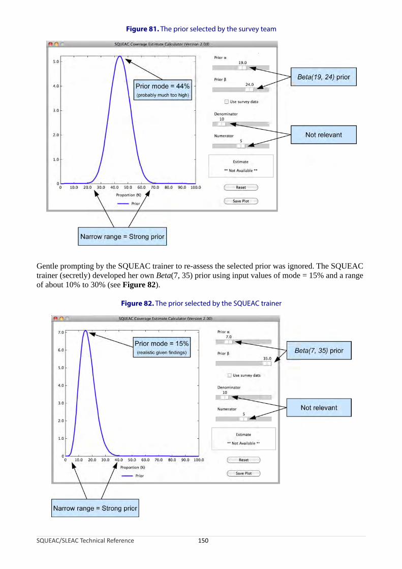
Figure 81. The prior selected by the survey team

Gentle prompting by the SQUEAC trainer to re-assess the selected prior was ignored. The SQUEAC trainer (secretly) developed her own Beta(7, 35) prior using input values of mode = 15% and a range of about 10% to 30% (see Figure 82).

Figure 82. The prior selected by the SQUEAC trainer


Using the survey team’s prior, a likelihood sample size of n = 54 cases was selected. This was calculated to yield an estimate with a precision of about ± 10 percentage points:

n = ⌈ 0.44 ×(1 − 0.44)2 −(19 + 24 − 2)

(0.1 ÷ 1.96) ⌉= 54

Using the SQUEAC trainer’s prior, a likelihood sample size of n = 9 cases would have been selected:

n = ⌈ 0.15 ×(1 − 0.15)+ 9

( 1.96)2−(7 35 − 2)

0.1 ⌉=÷

This was also calculated to yield an estimate with a precision of about ± 10 percentage points.

The likelihood sample returned:

Numerator : 9 current cases in the program

Denominator : 89 current cases (including current cases in the program)

Figure 83 shows the results of the beta-binomial conjugate analyses performed with the team’s Beta(19, 24) prior and the SQUEAC trainer’s Beta(7, 35) prior. The results of the two analyses are very different from each other.


Figure 83. Results of the beta-binomial conjugate analysis performed with the team’s Beta(19, 24) prior and the SQUEAC trainer’s Beta(7, 35) prior

A : Team’s prior and likelihood conflict

B : SQUEAC trainer’s prior and likelihood do not conflict

In the analysis performed using the team’s Beta(19, 24) prior there is no overlap between the prior and the likelihood, and the coverage estimate calculated using the likelihood survey data alone:

CoverageLikelihood =9

89× 100 =10.1 %

is very different from the prior mode of 44%. The prior and likelihood are said to conflict. When this happens, the results of the analysis are suspect and are usually discarded. In this case, the problem was caused by the use of a strong prior with an unrealistic mode. It is not reasonable to use the results of this analysis.


In the analysis performed using the SQUEAC trainer’s Beta(7, 35) prior there is considerable overlap between the prior and the likelihood, and the coverage estimate calculated using the likelihood survey data alone (10.1%) is not very different from the prior mode of 15%. The prior and the likelihood do not conflict. It is reasonable to use the results of the analysis.

The use of the unrealistic prior would have led to a gross overestimation of coverage. Checking for a conflict between the prior and the likelihood identified the problem and the misleading results were rejected. When this happens, a new prior needs to be defined (i.e., by re-examination of existing data and incorporation of the data collected for the likelihood survey) and a new likelihood survey undertaken. This is a lot of additional work. It is best to avoid the problem by being scrupulous and realistic when specifying the prior.

The mode of the prior chosen by the survey team was unrealistic in this case because they wanted the coverage to be high, and this led them to underestimate the effect of negative findings and overestimate the effects of positive findings. The survey team’s prior reflected what the team wanted the coverage to be rather than what the collected data indicated the coverage was likely to be.


Case Study: Sampling without Maps or Lists

This case study describes how a likelihood survey sample was taken in a SQUEAC assessment when neither maps nor useful village lists were available. A similar method could also be used for a SLEAC survey.

Figure 84 shows the most detailed map of the program area that was available at the time of the assessment. The map showed only district and sub-district boundaries. The shaded areas on the map represent the sub-districts in which the CMAM program was active. The filled circles on the map represent the approximate locations of CMAM clinic sites.

Figure 84. The most ‘detailed’ map available

s t ys mp vill g ial illa ea strved difficult because administrative boundaries, the names of administrative areas, and the

fficial names of villages had been subject to frequent change as the result of ongoing government r organisation. It was found that a large number of villages had official names that were different

om their everyday ‘folk names’ and were not recognised by residents. Village names recorded on tient records cards often did not match official village names.

fter spending 2 days trying to find villages using official names the assessment team decided that y needed to create their own list of villages. Interviews with program outreach workers validated informal group discussions in markets, guesthouses, ‘tearooms’, and at CMAM clinic sites

dicated that the ‘parish’ (i.e., the catchment area of a named church) was a stable areal designator at was readily recognisable by the entire population regardless of their religion. Key informants ogram outreach workers, priests, council leaders, and agricultural extension workers) were asked ist the parishes in their home sub-district. They were then asked to list the villages belonging to

ch of the listed parishes. A second list was made using different key informants. The two lists were mpared and discrepancies resolved with the assistance of a third, fourth, or fifth key informant.

he list was then (partially) checked for completeness by checking that all of the village names corded on patient records cards were also present in the list. This process resulted in a list of lages in each sub-district stratified by parish and validated by triangulation by source and method.


N

Attempt o take a s tematic sa le of ages usin an offic list of v ges in ch sub-di ict prooe

frpa

Atheby inth(prto leacoTrevil

A systematic sample was selected from this list:

• It was calculated that a sample of 40 villages was required.

• The list of villages was sorted by sub-district and parish (see Figure 85).

• There were 218 villages in the list, so a sampling interval of:

Sampling interval = ⌊ 21840 ⌋= ⌊ 5.45 ⌋ = 5

was used. A random starting position of 2 (selected using =RANDBETWEEN(1,5) in a Microsoft Excel spreadsheet) was used. This lead to a systematic sample of 44 villages being selected.

Figure 85. The list of villages was sorted by sub-district and parish

e ted ges e ed hou ho cre g se-t ho r was u because it was the case-finding method used by program outreach workers and each survey

m contained at least one program outreach worker who could share their experience with other embers of the team. The adoption of house-to-house screening reduced training overheads and

aved the time and effort required to develop and test an adaptive and active case-finding proced

llages close to a market town were not visited on the market day. Also, sampling did not take place days when CMAM sessions were held at the local CMAM clinic site.


Sub-district

Parish

Parish

Parish

Village

Village

Village

Village

Village

Village

Village

Village

Village

Sub-district

Parish

Parish

Parish

Village

Village

Village

Village

Village

Village

Village

Village

Village

District

Th selec villa wer sampl using se-to- use s enin . Hou o- use sc eening sed

teams ure.

Vion

The use of parish as the areal designator proved easy to use in the field. Teams started bng by the parish

y finding the parish church and were then directed to the villages selected for sampli priest or another church official.

Additional validation of the within-parish lists of villages with the parish priest or church official revealed very few errors. An additional seven small villages were identified (i.e., the list was estimated to be about 97% complete). These additional villages were not sampled.

The process of creating the list in each sub-district took 1 day. The process of creating the complete list, selecting the sample, and planning the fieldwork took 4 days.


Case Study: Using Satellite Imagery to Assist Sampling in Urban Settings

This case study illustrates the use of lists, maps, and satellite images when sampling for a likelihood survey for a SQUEAC assessment of program coverage in Mogadishu, Somalia.

A histogram prior was developed using routine program data, qualitative data, and the findings of small studies and small-area surveys. The prior had a mode of 60% with credible values ranging between about 40% and about 75%. Experimentation with the BayesSQUEAC calculator found that a prior defined as Beta(15.0, 10.3) provided a reasonable match to the histogram prior (Box 4).

Box 4. Using BayesSQUEAC to find α and β values that match a histogram prior


The minimum sample size required for the likelihood survey (nmin = 25) was calculated by simulation using BayesSQUEAC so that the expected likelihood had the same mode and the same strength and width as the prior (Figure 86). Calculating the minimum sample size in this way ensures that the sample size of the likelihood survey is sufficiently large to be able to correct a poorly specified prior.

Figure 86. Calculating a minimum sample size using the BayesSQUEAC calculator


Note: This approach will yield a similar (but not necessarily the same) value to that obtained using the formulasfor calculating the sample size for the likelihood survey presented in the SQUEAC section of this document

Sampling locations were selected using a spatial hierarchy:

ec org na hy pro m t wa orga d stric chf ub-districts each containing four locations. The city and the districts within the city had well-efined ‘official’ boundaries. Sub-districts and locations were program entities and, at the time of the QUEAC coverage assessment, had poorly defined boundaries. It was necessary, therefore, to create map of sub-district and location boundaries for the purposes of sampling.

o recent map of the city was available. A low-resolution satellite image of the city was available. strict boundaries were marked on this satellite image (Figure 87).


DistrictCity

Sub-district

Location

Location

Location

Location

Sub-district

Location

Location

Location

Location

Sub-district

Location

Location

Location

Location

Sub-district

Location

Location

Location

Location

that refl ted the anisatio l hierarc of the gra tha s nise by di t, ea with our s

dSa

NDi

Figure 87. District boundaries marked on a low-resolution satellite image

ghe olut llite s o in idu tri ha gra activ an d access at the time of the SQUEAC assessment were downloaded using Google Earth

( tp://earth.google.com). District boundaries were marked on these higher resolution ellite images (Figure 88).


Hi r res ion sate image f the div al dis cts t t the pro m was e in d coulsafelyht

sat

Figure 88. District boundary of Shingani district marked on a satellite image

Sub-district boundaries were decided by discussion with program staff and marked on the satellite image (Figure 89). Main roads, shorelines, rivers, drains and canals, and obvious landmarks were used to locate boundaries. This simplified fieldwork by making sub-districts and their boundaries easy to locate and sample.

Figure 89. Sub-district boundaries added to the satellite image of Shingani district


Lists of locations and their boundaries were decided by discussion with program staff using rough hand-drawn maps to focus discussion (Figure 90). Location boundaries were marked on the higher resolution satellite images of the districts (Figure 91). Again, main roads, shorelines, rivers, drains and canals, and obvious landmarks were used to locate boundaries. This simplified fieldwork by making locations and their boundaries easy to locate and sample.

Figure 90. Rough hand-drawn map use to create lists of locations by sub-district


Figure 91. Location boundaries added to the satellite image of Shingani district

At the end of this process, there was a set of district maps showing sub-district and location boundaries. These maps were translated into a list of locations sorted by district and sub-district (Figure 92).

Figure 92. List of locations sorted by district and sub-district created from the mapping process (also showing systematic sampling with start = 3 and interval = 9)

Note: The sampling interval is applied until the end of the list is reached. In this example the methodselected 11 sampling locations. All 11 locations were sampled.

Shingani

Hawd

Mooyale

Midnimo

Jabuuti

DegmadaFiimoSportigaCurubaBaer ItaliaSharif AbowDalsanSharud ZenowCaymiskaBortamahaJubbaIshimaMadbacaddaHawlaha MareekubtaSafeeroda EtobiaGiisha Baraa

Waberi

Hawl Wadaag

Xawo TakoLulyoJabuuti26 Juun

Horseed

HillacIskaashiAdariHalgan

Ida Mayo

Ahmed Gurey1 MayMohamed HassanBolotikniko

October

XoogeWajeerJ. Da'udDhagextuur

Wadajir

Hawo Tako

NasteexoHilaacGelowAli Hussein

Tima Cadde

HeeganAargoSudiHassan Jiis

J. Da'ud

Buula XubeyDanwadaagahaWasaradda MacdenBadaadir Hospital

Xalane

TimankaQurunbowHorseedAdon Gabyow

Dharkeynley

Xanaono

1 aad2 aad3 aad4 aad

Dhagaxfur

XooshWarshsadaGaras BaalayNuur Aduunyo

Sacud Reorge

DahageynkoShawridaAbe GeddoKaxda

Dhamme Yasun

HeganHalgariHorseedIftin

Hamar-Jajab

Gahayr

Horseed

J. Da'ud

Ida Mayo

XaleneSh'ShaacirAhmed GureySaqawadinMohamud HorbiWajeerNashib BundoHawass26 JuunIda JulyIftimTaleexAhmed GureyJabuuti12 OctoberId Luulyo

Hamar-Weyne

Gobamimo

KoodkaCadaygaW'LacoqteBuur Fuule

Kacaan

AweyskaVia RomeYunlayeAweys Geedow

Horseed

RapaygaBinguberCadule ShideyaDacarey

Hilaac

YoobsenMacian JacmocVia EjatoHawo Take

•

•

•

•

•

•

•

•

•

•

… from previous column

to next column ...

+ 9

+ 9

+ 9

+ 9

+ 9

+ 9

+ 9

+ 9

+ 9

+ 9

A systematic sample was taken using this list. The number of locations to sample was calculated using the standard formula:

nlocations =⌈ n

average location populationall ages ×percentage of population6 – 59 months


100 ⌉


The average population in each location was estimated to be 500 people, the percentage of the population aged between 6 and 59 months was estimated to be 20%, and SAM prevalence estimated to be 2.5% (this was taken from a recent nutritional anthropometry survey) giving:

nlocations =⌈ 25

500 × 20100 × 2.5

100 ⌉= 10

The sampling interval was calculated as:

Sampling Interval = ⌊ Total number of locationsNumber of locations to sample ⌋= ⌊ 96

10 ⌋= ⌊9.6⌋ = 9

A random sample location was selected using a random number between 1 and 9 generated using coin tosses. The generated random number was 3, so the third location on the list was selected. The method for generating random numbers by tossing coins is described under “A Note on Generating Random Numbers” in the SQUEAC section of this document. Subsequent sampling locations were selected by repeated addition of the sampling interval. This process (see Figure 92) ensured that the sample was distributed over the entire program area. Figure 93, for example, shows the two locations selected for sampling from Shingani district.

Figure 93. Locations in Shingani district selected for sampling


Selected locations were sampled using building-to-building and door-to-door sampling to account for multiple occupancy of compounds and buildings. Satellite images, such as the one shown in Figure 94, provided sufficient detail to allow fieldworkers to reliably identify locations, location boundaries, and dwellings in each of the selected locations.

Figure 94. Satellite image showing a single sampling location


Case Study: Active and Adaptive Case-Finding in a Rural Setting

This case study describes the procedure used to conduct active and adaptive case-finding (see Box 3, page 65) during SQUEAC investigations in two rural districts of Niger.

The case-finding method described here was used for both the small-area surveys and the likelihood survey and was based on the following two principles:

The method is active. SAM cases were specifically targeted. Case finders did not go house to house in the selected villages measuring all children aged between 6 and 59 months. Instead, only houses with children with locally understood and accepted descriptions of malnutrition and its signs were visited.The method is adaptive. At the outset, key informants helped with case-finding in the community, but other sources of information found during the survey were used to improve the search for cases.

Preparatory Research

For the active and adaptive case-finding method to be effective, research must be conducted during the qualitative phase of the SQUEAC investigation to determine:

• The appropriate case-finding question• The most useful key informants to assist with case-finding•

he C

Any context-specific factors affecting the case-finding process

T ase-Finding Question

Appropriate local terminology used by the population to describe the signs of SAM had to be identified and community definitions and aetiologies understood so that these could be used to facilitate the active search for cases. Carers of children with SAM enrolled in the CMAM program and carers of children recovering from SAM enrolled in the CMAM program were asked:

• To describe the condition of their child• What terms should be used and how the signs should be described in local languages if we

wanted to find children with the same condition in other villages• To explain the signs and symptoms that led them to consult the CHW or attend the health

centre

Pictures of children with SAM were shown to a wide variety of community members who were asked to name the local terms for particular signs (e.g., skin signs, hair signs, baggy-pants, thin arms, swollen feet), the conditions (i.e., severe wasting and kwashiorkor), and their causes. Care was taken to identify derogatory and insulting terms.

The research indicated that the following terms were understood and used by the community to describe children with malnutrition:

• Tamowa (flaccid and/or wrinkled skin)• Kwamaso and kwameshewa (wasting)• Raama (thin, wasted)• Tsimbirewa (child is small and resembles an old man)• Koumbiri (swelling)


The research also revealed that malnutrition was not always recognised as a specific condition but as the outcome of illnesses (predominantly diarrhoea and fever). It was considered important, therefore, to ask for children that currently had or were recovering from conditions such as:

• Masas sara (fever)• Zawo (diarrhoea)

It should be noted that the information collected while determining the appropriate case-finding question is often useful in other aspects of a SQUEAC or SLEAC investigation. For example, these findings should be compared with program messages. If program messages do not match all of these findings (e.g., the program messages do not explicitly mention diarrhoea and fever or exclude some local language terms), there may be a negative impact on coverage. Also, if program messages use derogatory or insulting terms, there may be a negative impact on coverage, since not many people would proudly identify themselves as, for example, dirty, ignorant, drunken whores.

Identifying Key Informants

It was necessary to identify the types of people who, because of their position in the community or their contact with and knowledge of small children, were likely to be able to identify SAM children.

Such key informants would be able to direct survey teams to the homes of potential SAM cases and avoid the need to conduct a house-to-house search for SAM cases. Specifically:

Carers of children with SAM enrolled in the CMAM program and carers of children recovering from SAM enrolled in the CMAM program were asked:

Who would know which children were sick or had the same condition as your own child in the village and could help us find cases?

A wide variety of community members were asked:Who in your village is best placed to tell us about the health of young children and to know which children are sick?

Treatment-seeking behaviours were also explored to see which people were first consulted for help and advice when a child became sick or wasted.

The following people were identified as useful key informants:The matrone (senior TBA in a village)The kungiya (women’s leader)Grandmothers and respected older womenVillage and religious leadersTraditional health practitionersVillage pharmacists

It should be noted that this information is often useful in other aspects of a SQUEAC or SLEAC investigation. For example, these findings should be compared with the types of people that are recruited as community-based case-finders or that are regularly and frequently contacted in program outreach activities. If some types of people are not recruited as community-based case-finders or are not in regular and frequent contact with the program, there may be a negative impact on coverage. Also, if carers initially seek treatment with traditional health practitioners and traditional health practitioners are not recruited as community-based case-finders or are not in regular and frequent contact with the program, there may be negative impact on coverage.


Context-Specific Factors Affecting the Case-Finding Process

Any potential cultural or practical constraints that could influence the conduct of the case-finding haif

d to be identified to ensure that these were taken into account and the method adapted accordingly necessary. Specifically:•

•

•

Community members were asked about daily activity patterns so as to inform timing of case-finding activities (e.g., to know when carers and children are likely to be at home, to avoid sampling at meal times or on market days).Cultural norms regarding the acceptability of male case-finders speaking to women and entering houses and compounds were discussed with the SQUEAC team and verified during village visits.Observations were made with respect to the general structure of villages.

Nanho

o major constraints were identified. However, findings showed that it was important to establish if y hamlets were attached to the village or if the village was made up of more than one cluster of uses so that these populations were not overlooked during sampling.

Survey Stage

Active and adaptive case-finding proceeded in the following way in each village selected for the surveys:

1. The survey team presented themselves to the village leaders and requested the help of a key informant.

2.

3.

The case-finding question and, in addition, knowledge of children attending a feeding program were asked of the key informant.The team arrived at the first house indicated by the key informant and, after checking that the identified child was aged between 6 and 59 months and explaining the purpose of the visit to the carers, the team measured the identified child as a potential case.

4. If the child was found to be a SAM case, confirmation was sought as to whether the child was enrolled in the CMAM program. If the child was not in the CMAM program, then a short questionnaire (similar to that shown in Box 2, page 49) was administered to discover the reasons for coverage failure and the child was referred to the nearest CMAM program site. If the child was not currently a SAM case, confirmation was sought as to whether the child was enrolled in the CMAM program to check whether the child was a recovering SAM case.

5. All cases identified (i.e., covered and uncovered SAM cases and recovering SAM cases in the CMAM program) were noted on a tally sheet.

6. Before proceeding to the next potential SAM case known to the key informant, the carers of the case just identified were asked if they knew of any children with a similar condition or who were in a feeding program.

Case-finding was considered to be exhaustive when no new leads to potential cases were forthcoming and when information given by different sources (e.g., key informants and carers) identified children that had already been seen by the team.

The survey process is summarised in Figure 95.


Figure 95. The survey process using active and adaptive case-finding


Ask the village leader to provide you with a key informant of your choosing

Ask the key Informant the case-finding question

Go to the first house where a potential case may be found

Check the child is aged between 6 and 59 months

Explain the purpose of the survey to the parents and what you will do

Measure the MUAC of the child

Check for the oedema sign

Does the child have bilateral oedema or is the MUAC < 115 mm?

Use additional sources or other key informants to inform and improve the search

Always ask parents of SAM children identified whether they know of other cases

Continue until no new cases are indicated by any source or all leads point to previously identified cases

Fill out the tally sheet

Apply questionnaire

Refer the child to CMAM program site

Thank the mother

Ask case-finding question

Current SAM case not in program

Current SAM case

Is the child in the OTP?

Ask to see sachet of RUTF and health card

Not a current SAM case

Is the child in the OTP?

Ask to see sachet of RUTF and health card


Thank the mother


Current SAM case in program Recovering SAM case


Thank the mother


Observations

The case-finding method targeted SAM cases and recovering SAM cases. Case-finding was quicker and more effective than if a blanket screening method had been used. It was possible for each survey team to sample at least two villages per day, even when villages had more than 3,000 inhabitants.

Using familiar terms and definitions understood by the community enabled a large number of cases to be identified, including many severe kwashiorkor cases whose condition had not been recognised as malnutrition.

Potential cases were identified that were not in the village at the time of the survey because they had gone to a CMAM program site. The names of these children were checked on the CMAM register in the health centre at the end of the day and their current measurements verified on the beneficiary card to determine whether they were current or recovering SAM cases.

The matrone (the senior TBA in a village) proved to be a very useful key informant and was the usual starting point. Her knowledge was often supplemented by that of the kungiya (women’s leader) as the search progressed.

A snowball effect was often seen once the first SAM case was identified. The carer of the first case gave information on another child with the same signs as her own, the carer of that case and their neighbours in turn gave leads to further potential cases, the carers of these cases in turn knew of other cases, and so on.

During the search, a number of carers with uncovered SAM cases also approached the case-finding team, having heard of the survey from others in the village.

Summary

Before undertaking active and adaptive case-finding determine:

The case-finding question. Appropriate definitions, terms, and descriptions for malnutrition, its signs, and its aetiology in the local language(s).

Key informants. People that have frequent contact with small children or know which children are or have recently been sick.

Context-specific factors affecting the case-finding process. These are cultural or practical constraints that need to be considered.


Case Study: Within-Community Sampling in an Internally Displaced Persons Camp

This case study describes an application of active and adaptive case-finding in IDP camps. A SQUEAC investigation was carried out in two IDP camps, Adn and Nu’ma, in a north African country to assess coverage for an established NGO-implemented TFP. The surveys reported here are small-area surveys of suspected low coverage areas, but the approach used and the lessons learned could be applied to wider-area likelihood surveys in similar settings.

Challenges and Constraints

An initial investigation identified two challenges to within-community sampling in the camps:

1. The physical and social boundaries of ‘communities’ in the camps were not known.

2. There was an absence of persons typically recruited as key informants to assist with case-finding.

Security constraints also limited access to the camps.

Physical and Social Boundaries of Communities

Adn and Nu’ma camps were nominally divided into ‘sectors’. Each sector accommodated the influx of a new group of IDPs. A sector was not a cohesive unit, but was composed of a set of smaller communities based on pre-displacement community of origin. Each community identified with a particular sheikh (village leader). Sector numbers were not recorded in the OTP registration book because these were were often not known to carers. The name of the sheikh was, however, always recorded.

The influx of large numbers of IDPs resulted in organic growth. Individual sectors and communities were not clearly delineated and ‘official’ sector boundaries varied both within and between agencies working in the camps. There was no obvious structure in terms of the arrangement of streets and houses in the camps. Communities were not always accommodated together and some were dispersed throughout the camp. The population and extent of each community was not, therefore, immediately or easily identifiable.

The reproduction of home communities also meant that, although some new acquaintances were made, it was common for people to have limited knowledge of and contact with members of neighbouring households if they belonged to different communities. Initial case-finding efforts in Nu’ma camp proved ineffective until it was realised that the failure to find SAM cases in a particular area of the camp was due to the informant’s lack of knowledge of people that they lived in close proximity to but who belonged to different communities.

Absence of Typical Key Informants

The need to gain an income meant that looking for work and maximising opportunities for casual labour were household priorities. People tended to leave the camps during the day to find work in neighbouring towns. Many houses stood empty or were occupied only by children during the day.

The need for income also applied to those in positions of responsibility. These included many of the key informants that are typically used for active and adaptive case-finding in SQUEAC investigations. TBAs were prohibited from working as midwives in the camps.

It was not possible to survey in the evening, when many would have returned from work in the town, due to security restrictions.


Active and Adaptive Sampling

One sector was selected for assessment of coverage by small-area survey in each camp. These sectors were selected because routinely collected and qualitative data indicated that coverage was likely to be low in these sectors.

Adn – Sector 5 Nu’ma – Sector 7

Vulnerable sector: High population movement:

• Many recent arrivals • Daily workers to local towns

• Poor sanitation and hygiene • High numbers of defaulters

• Risk of flooding • Many children left alone or with neighbours

Pockets of malnutrition identified by screening Small number of admissions for population size

Very few admissions to CMAM program Low awareness of malnutrition

Very low awareness of malnutrition Low awareness of the CMAM program

Very low awareness of the CMAM program Large number of women-headed households

Neglected sector: Large number of children-headed households

• No responsible NGO

• Focus of activities on Sector 10

• Known poor coverage of general ration

Each sector contained 100 or more communities.

Communities were mapped by a process of determining belonging (see below).

Case-finding was done using community-specific informants identified by social network analysis (see below).

Mapping by Determining Belonging

To ensure that case-finding was exhaustive, each community in the selected sector was sampled separately, assisted by informants specific to that community. The number and location of houses belonging to each community was established and boundaries were continually reconfirmed during the exercise to avoid:

a. Eligible houses being missed

b. Straying inadvertently into a different community

c. Getting lost

This mapping of communities involved moving from house to house and asking:

Which sheikh do you belong to?

Do the adjacent houses belong to the same sheikh?

Are there people that belong to the same sheikh but that live in a different part of the camp?

Communities were sampled one at a time using key informants specific to each community.

Communities were not ‘mapped’ in the usual sense of the term (i.e., a diagrammatic representation of an area drawn on paper). The process of mapping was dynamic, with community boundaries located and membership confirmed during case-finding by constant questioning. This way a working mental map of communities was built up.


Exploit Social Networks for Case-Finding

Social networks were explored to facilitate the identification of potential SAM cases when no obvious key informant was available. Family members of persons typically recruited as key informants in SQUEAC assessments were recruited because they often shared knowledge of the wider community. Some women were able to provide information that extended beyond their immediate neighbours because they were often linked in both formal and informal ways. Faced with a common problem, social ties had frequently been strengthened and groups of women would join together to travel in safety to undertake work outside of the camps. Similarly, they would take turns collecting rations to enable others to continue working. A number of women also participated in NGO-organised craft activities and, as a consequence, widened their social networks.

Although they were no longer practising, the continued friendship of TBAs with different families proved useful in identifying potential cases. Common interests also drew wider groups of people together at water points, shops, and ceremonies (e.g., christenings, marriages, and funerals), which often transcended community boundaries. The awareness and contacts of people found at these sites were also exploited to ensure exhaustive sampling. Communities were sampled one at a time using informants specific to each community. These informants were identified and recruited as case-finding moved from community to community.

Lessons Learned

Conducting a SQUEAC assessment in these camps raised a number of sampling issues and underlined the importance of adapting methods to the particular context. Case-finding methods need to be designed and adapted for specific contexts. There is no guarantee that a method that works well in one setting will work well in another.

For future SQUEAC investigations in camp settings the following steps are recommended:

• Allow time to understand the complexities of camp structure.

• Allow time to understand the social and economic realities of camp life.

• Allow time to identify and map individual communities during case-finding.

• Allow time to identify and recruit (key) informants during case-finding.

Conclusions

It should not be assumed that active and adaptive case-finding methods that usually work well in rural communities will also work in other settings. Our experience is that active and adaptive sampling can work in IDP camps, but only if efforts are made to identify and map communities and social networks during case-finding.


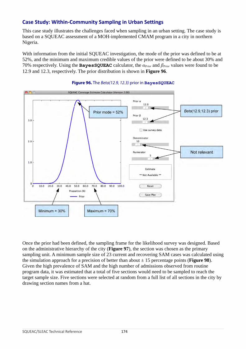
Case Study: Within-Community Sampling in Urban Settings

This case study illustrates the challenges faced when sampling in an urban setting. The case study is based on a SQUEAC assessment of a MOH-implemented CMAM program in a city in northern Nigeria.

With information from the initial SQUEAC investigation, the mode of the prior was defined to be at 52%, and the minimum and maximum credible values of the prior were defined to be about 30% and 70% respectively. Using the BayesSQUEAC calculator, the αPrior and βPrior values were found to be 12.9 and 12.3, respectively. The prior distribution is shown in Figure 96.

Figure 96. The Beta(12.9, 12.3) prior in BayesSQUEAC

nce the prior had been defined, the sampling frame for the likelihood survey was designed. Based n the administrative hierarchy of the city (Figure 97), the section was chosen as the primary am ng it. mi um am e si of 2 curr nt rec rin A ca wa lc ed u ng he simulation approach for a precision of better than about ± 15 percentage points (Figure 98). iven the high prevalence of SAM and the high number of admissions observed from routine rogram data, it was estimated that a total of five sections would need to be sampled to reach the rget sample size. Five sections were selected at random from a full list of all sections in the city by awing section names from a hat.


Oos pli un A nim s pl ze 3 e and ove g S M ses s ca ulat sitGptadr

Figure 97. Administrative hierarchy of the city


Local GovernmentArea (LGA)

Ward

Ward

Ward

Section

Section

Section

Section

Section

Section

Section

Figure 98. Sample size by simulation approach using BayesSQUEAC

Different numerators and denominators are tried until the displayed estimate shows the required precision

The active and adaptive case-finding method (see Box 3, page 65) was used for within-section sampling in each of the five selected sections. The district or ward heads served as the community entry points and were consulted to determine the boundaries of the selected sections. Once the boundaries were determined, the sections were divided into smaller geographical blocks in which different survey teams were assigned to conduct case-finding. This was initiated by locating identified key informants, such as district or ward heads, imams or sheikhs, TBAs, traditional healers or wanzami (persons who perform circumcisions). Key informants were asked whether they knew of children suffering from olu, tamuwa, sefa or nono (the terms that most people in the city use for children that are very thin or have distended abdomens, brownish or discoloured hair, and scaling of the skin) or children that had kumburi (the term used for children with kwashiorkor). In addition, the key informants were asked if they knew of children that had kurga, a condition in which the child is passing loose or watery stools and was associated by most local people with wasting and kwashiorkor. If they knew of such children, they were asked to lead the team to the children’s homes, where the children were examined and their MUACs measured. The same case-finding questions described above were asked of carers of children examined and of other key informants identified. This process was repeated until all identified key informants had been consulted.

Active and adaptive case-finding was unsuccessful in this context. Only five current and recovering SAM cases were found. During the case-finding process, key informants were unable to lead the survey teams to more SAM cases despite high prevalence in the area and many current cases in the program at the time of the survey reported to be living in the selected sections. One possible explanation for this failure is that social dynamics in a big town or city are different from those in villages or rural areas, where active and adaptive case-finding has been shown to work well. The method is based on the assumption that the community being sampled has considerable social connections amongst its members. In large towns and cities, such assumptions often do not hold true.

As can be seen in Figure 99, the posterior distribution is only marginally stronger/narrower than the prior distribution. This is because the small sample size likelihood adds little new information to inform the posterior. The effect of not finding enough SAM cases on the coverage estimate is that the coverage estimate is dominated by the prior. The prior and likelihood do not conflict so any bias is likely to be small.

The problems finding cases suggests that building-to-building and door-to-door sampling would have been better in this urban setting and should probably be used as an alternative to active and adaptive case-finding in situations where the assumption of social connectedness amongst people in the survey area is uncertain.


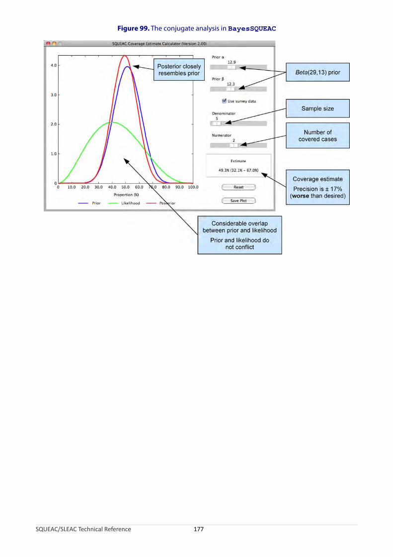
Figure 99. The conjugate analysis in BayesSQUEAC


Case Study: The Case of the Hidden Defaulters

This case study describes how a SQUEAC investigation identified and investigated the issue of ‘hidden defaulters’ in a CMAM program implemented in a southern African country by the MOH supported by an international NGO.

Routine program monitoring data were analysed. A plot of admissions over time revealed that the program was probably responsive to need. Rises in admissions coincided with periods when SAM incidence was expected to be high (e.g., during periods of food insecurity and of increased incidence of infections associated with wasting). The results of the analysis of program exits were consistent with a well-performing program. Cure, default, and death rates were all within Sphere minimum standards:

Cured : 81%Default : 8%Transfers to hospital : 9%Deaths : 2%

Qualitative data revealed that carers heard of the CMAM program from their local health centres and through program-sponsored announcements on local radio. Carers of children in the program and other informants reported that they were unaware of malnourished children in their communities that were not already covered by the program.

The quantitative and qualitative data described above were consistent with a program achieving moderate or high levels of coverage.

During mapping of home locations of beneficiaries using data from admission records, a considerable number of record cards with only one or two visits recorded were found. It was suspected, therefore, that there was likely to be considerably more defaulting than was recorded in the routine program monitoring data. Interviews with program staff revealed that program activity had focussed on delivering services to beneficiaries at clinics and that absences were not well recorded. This had led to an under-reporting of defaulters. These findings prompted an investigation focussed on defaulting.

Current and past beneficiary record cards were examined and discharges classified according to the program’s own discharge criteria. This exercise resulted in a very different picture of the program:

Cured : 40%Default : 49%Transfers to hospital : 9%Deaths : 2%

Further analysis revealed that a large majority (approximately 90%) of defaulters defaulted after only one or two visits to a program site (Figure 100). These were early defaulters and, therefore, probable current SAM cases at the time of defaulting.


Figure 100. Number of visits before defaulting

1

2

3

4

≥ 5

20 40 60 80 100 120 140

Number of defaulters

Nu

mbe

r of

vis

its


The trend of defaulting over time was analysed. This revealed that defaulting peaked during periods of higher agricultural labour demand (Figure 101).

Figure 101. Trend of defaulting over time

xam e c aul

The majority of active cases came from villages within 5 km of program sites.

The majority of defaulters came from villages farther than 5 km from program sites.


Malaria

Diarrhoea

ARIs

Clearing/Sowing Harvest Clearing/Sowing

Rainy season Rainy season

Peaks of defaulting when agricultural workload higher

Jan Feb Mar Apr May Jun Jul Aug Sep Oct Nov Dec0

10

20

30

40

50

60

E ination of the home locations of activ ases and def ters (Figure 102) indicated that:

•

•

Figure 102. Distance from home to a CMAM program site for active cases and defaulters

h fin ng p b n r w t d u e ie t n reported that the most important factors affecting their decision to default was the amount of

cultural work that they had to do (i.e., the higher the workload the more likely they were to default) and the distance between their homes and the program sites. It should be noted that these

ere not independent findings since time-to-travel is an opportunity cost (longer times to travel to he program sites mean less time for work).

hese new findings caused the SQUEAC investigators to revise their initial belief of moderate to gh program coverage and changed the focus of the investigation report and recommendations.

his case study highlights the importance of:• epticism when working with routine program monitoring data. In this case, defaulting was

rossly under-reported.• nvestigation and the triangulation process in ensuring the robustness of findings. In this case,

he investigators were presented with conflicting data (i.e., routine program monitoring data howed low levels of defaulting but coverage mapping suggested high levels of defaulting).

This prompted further investigation using a variety of sources and methods (i.e., triangulation y source and method).


T ese di s were sup orted y i te vie s wi h carers of efa lt d pat n s. These key i formants

agri

wt

Thi

TScgIts

b

Case Study: Applying SLEAC: Sierra Leone National Coverage Survey

The CMAM approach to treating cases of SAM in government health facilities was piloted in four districts of Sierra Leone in 2008. The program was expanded to provide CMAM services in selected health centres in all 14 districts of the country in 2010. This case study describes the application of SLEAC to the assessment of the coverage of this national CMAM program.

SLEAC Sampling Design

SLEAC was used as a wide-area survey method to classify coverage at the district level. The district was selected as the unit of classification because service delivery of the national program was managed and implemented at the district level.

The PSUs used in the SLEAC surveys were census enumeration areas (EAs). In rural districts, EAs were individual villages and hamlets. In urban and peri-urban districts, EAs were city blocks. In rural districts, lists of potential PSUs were sorted by chiefdom. In urban and peri-urban districts, lists of potential PSUs were sorted by electoral ward (sections). This approach ensured a near-even spatial spread of the selected villages across rural districts and a near-even spatial spread of selected EAs across urban and per-urban districts. The structure of the district-level samples are shown in Figure 103.

Figure 103. Structure of samples in rural and peri-urban/urban districts

t et m e ze n 0 re S se a ed b h n rb di ct T s the standard SLEAC sample size for large populations. A lower target sample size (n = 33) was used

the single peri-urban district because this district had a much lower population than the other istricts.


District

Chiefdom

Chiefdom

Chiefdom

District

Section

Section

Section

Village

Village

Village

Village

Village

Village

Village

Village

Village

Village

B : Urban and peri-urban districtsA : Rural districts

City Block

City Block

City Block

City Block

City Block

City Block

City Block

City Block

City Block

City Block

A arg sa pl si of = 4 cur nt AM ca s w s us in ot rural a d u an stri s. his i

in d

The number of PSUs (nPSU) needed to reach the target sample size in each district was calculated using estimates of average EA population and SAM prevalence using the following formula:

target samnPSU =⌈ ple size (n)

percentage of populationaverage EA population 6 – 59months SAM prevalence

all ages × ×100 100 ⌉

Average EA population was estimated as:

District populationAverage EA population =

Total number of EAs in the district

using data from the most recent (2004) Sierra Leone Population and Housing Census.

The percentage of the population aged between 6 and 59 months was estimated as 17.7%. This is a national average taken from the Sierra Leone 2004 Population and Housing Census. This estimate was used by Sierra Leone government departments, United Nations organisations, and NGOs.

SAM prevalences were taken from reports of SMART surveys of prevalence in each district that had been undertaken in the lean period of the previous year. The prevalence of SAM using MUAC and oedema was used since this matched program admission criteria.

The Sierra Leone Central Statistics Bureau provided information on the total district populations and total number of EAs in each district. The Sierra Leone Central Statistics Bureau also provided lists of EAs for the Western Area (urban and peri-urban) districts and large-scale maps (see Figure 104) of the EAs that were selected for sampling.


Figure 104. Example of a large-scale map showing enumeration area boundaries used when sampling in an urban district

Map courtesy of the Sierra Leone Central Statistics Bureau

PSUs were selected using the following systematic sampling procedure:

Step 1. The lists of EAs were sorted by chiefdom for rural districts and by section for urban and peri-urban districts.

Step 2. A sampling interval was calculated using the following formula:

NumSampling interval = ⌊ ber of EAs in district

nPSU ⌋Step 3. A random starting PSU from the top of the list was selected using a random number between 1 and the the sampling interval. The random number was generated by the coin-tossing method described under ‘A Note on Generating Random Numbers’ in the SQUEAC section of this document.


The PSUs selected by this procedure were sampled using a case-finding method tailored to the particular district:

• In rural districts, a district-specific case-finding question was developed from the base case-finding question:

Where can we find children that are sick, thin, have swollen legs or feet, or have recently been sick and have not recovered fully, or are attending a feeding program?

This question was adapted and improved using information collected from TBAs, female elders, traditional health practitioners, carers of children in the program, and other key informants to include local terms (in all local languages) and local aetiological beliefs regarding wasting and oedema. This question was used as part of an active and adaptive case finding method (see Box 3, page 65).

• In urban and peri-urban districts, house-to-house and door-to-door case-finding was used. This was done because it was felt that active and adaptive case-finding would not work well in these districts. Sampling was aided by the use of large-scale maps showing EA boundaries provided by the Sierra Leone Central Statistics Bureau (see Figure 104).

After all selected PSUs in a district had been sampled, the survey team met at the district headquarters for data collation and analysis. The simplified LQAS classification technique was applied to the collated data.

The coverage standards:

Low coverage: Below 20%

Moderate coverage: Between 20% and 50%

High coverage: Above 50%

were decided centrally by MOH and UNICEF staff before the start of the surveys. These standards were used to create decision rules using the rule-of-thumb formulas:

d 1 = ⌊ n × p 1 ⌋ = ⌊n × 20100 ⌋= ⌊ n

5 ⌋ and d 2 = ⌊ n × p 2 ⌋ = ⌊n × 50100 ⌋= ⌊ n

2 ⌋where n is the sample size achieved by the survey, p1 is the lower coverage threshold (i.e., 20%), and p2 is the upper coverage threshold (i.e., 50%).

Coverage in each district was classified using the algorithm presented in Figure 70. Table 11 presents the results of the surveys. Figure 105 presents the same results as a map of per-district coverage.


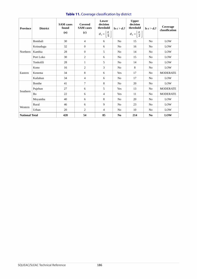
Table 11. Coverage classification by district

Province DistrictSAM cases

found

(n)

CoveredSAM cases

(c)

Lowerdecision

threshold

d 1 = ⌊ n5 ⌋

Is c > d1?

Upperdecision

threshold

d 2 =⌊ n2 ⌋

Is c > d2?Coverage

classification

Northern

Bombali 30 4 6 No 15 No LOW

Koinadugu 32 0 6 No 16 No LOW

Kambia 28 0 5 No 14 No LOW

Port Loko 30 2 6 No 15 No LOW

Tonkolili 28 1 5 No 14 No LOW

Eastern

Kono 16 2 3 No 8 No LOW

Kenema 34 8 6 Yes 17 No MODERATE

Kailahun 34 4 6 No 17 No LOW

Southern

Bonthe 41 7 8 No 20 No LOW

Pujehun 27 6 5 Yes 13 No MODERATE

Bo 22 6 4 Yes 11 No MODERATE

Moyamba 40 6 8 No 20 No LOW

WesternRural 46 6 9 No 23 No LOW

Urban 20 2 4 No 10 No LOW

National Total 428 54 85 No 214 No LOW


Figure 105. Map of per-district coverage

sh es re, r t a wn Bo pa 49) g a ut b rrie to era wstered to carers of non-covered cases found. Data were tabulated from the questionnaires

ng a tally sheet and presented as a Pareto chart (Figure 106).


Koinadugu

Bombali

Tonkolili

Kono

Kambia

Port Loko

Moyamba

BoKenema

Kailahun

Pujehun

Bonthe

Western

Low (< 20%)

Moderate (20% to 50%)

High (> 50%)

Peri-urban

Urban

Legend

A ort qu tionnai simila o th t sho in x 2 ( ge askin bo a rs cov ge as adminiusi

Figure 106. Barriers to service uptake and access

Lack of knowledge about the program

Lack of knowledge about SAM

No RUTF

Distance

No time/too busy

Discharged then relapsed

Other reasons

Previously rejected

0 50 100 150 200 250 300

Number

SLEAC Implementation Process

The process as described above was completed in 8 weeks (44 working days) staffed by 15 mid-level health management staff and a principal surveyor provided by Valid International. Three survey teams with five members each were used. The teams were divided into two sub-teams. A survey team was headed by a ‘captain’ who was in charge of managing the sub-teams, organising travel and survey logistics, and co-ordinating survey activities with the principal surveyor.

Each district was divided into three segments. Segmentation was informed by logistics, with each segment being served by a road (when possible).

Each survey team was assigned to one of the three segments and provided with:• A list of PSUs (sorted my chiefdom) to be sampled• A list of the locations of CMAM program sites• A list of the names and home villages of chiefs and chief’s assistants for each PSU to be

sampled

Eafor

ch survey team started case-finding in the farthest PSU and then moved to the next-farthest PSU case-finding and so-on. At the end of each day, the survey teams lodged in health centres, local

guunthesta

esthouses, or in villagers’ homes. They restarted case-finding on the following day. This continued il all the PSUs had been sampled. The survey teams then came together at the district

adquarters for data collation and analysis and results shared with district-level health management ff.

Upon completion, the survey team was able to:• Classify coverage in each district (Table 11, page 185)• Map coverage by district for the whole country (Figure 105)• List barriers to coverage ranked by their relative importance (Figure 106)


An overall coverage estimate was calculated but not reported. Figure 107 shows the calculation of a weighted point coverage estimator using spreadsheet software.

Figure 107. Calculation of a wide-area coverage estimate


Appendix 1. Technical Appendix

This appendix provides additional technical information regarding the choices of methods that are used in SQUEAC and SLEAC.

Active and Adaptive Case-Finding

The active and adaptive case-finding method (see Box 3, page 65) was originally developed for use in CSAS coverage surveys. Active and adaptive case-finding was tested during the development of the CSAS coverage survey method using capture-recapture studies. It was also common practice to test active and adaptive case-finding procedures using capture-recapture studies when the CSAS coverage survey method was used to assess program coverage in a particular area for the first time. These tests found that, when well done, the active and adaptive case-finding method:

• Finds all or nearly all SAM cases in sampled communities

• Consistently performed better than central-location screening and house-to-house screening

• Performed as well as house-to-house screening with local informants and verbal household censuses at finding sick or sleeping children that may be ‘hidden’ to avoid them being disturbed by the survey team

• Is more efficient than other case-finding methods

It should be noted that these findings apply only to using the active and adaptive case-finding method to find cases of SAM.

The active and adaptive case-finding method has been tested for finding cases of moderate acute malnutrition (MAM) and has been found to perform considerably worse than house-to-house screening. If SQUEAC or SLEAC are used to assess the coverage of, for example, an SFP, then house-to-house screening should be used and extra time allocated to survey activities.

The active and adaptive case-finding method has been known to fail in some urban and camp settings. Some examples of this may be found in the case studies section of this document. In such settings, it is advisable to use house-to-house screening and allow additional time for survey activities.

When finding cases of SAM using house-to-house screening, it is advisable to use local informants and to take a (verbal) household census before asking to measure children. This avoids the problem of sick or sleeping children being ‘hidden’ to avoid them being disturbed by the survey team.

Calculating the Required Likelihood Survey Sample Size

The formula for calculating the sample size for a likelihood survey is:

mnLikelihood =⌈ ode ×(1 − mode )

− (α +β − 2)(precision ÷ 1.96)2 Prior Prior ⌉

where mode is the mode of the prior, αPrior and βPrior are the shape parameters of the prior, and precision is the precision (i.e., the approximate half-width of the 95% credible interval) required for the posterior estimate.


The first part of the formula:

mode × (1 − mode )(precision ÷ 1.96)2

is the standard formula for calculating the required sample size for a survey with a non-informative prior. The value 1.96 closely approximates the standard normal deviate for the 97.5th percentile point of the standard normal distribution and is used to specify a 95% credible interval. Other values (e.g., 2.58 for a 99% credible interval) may be used.

The second part of the formula:

(αPrior +βPrior − 2)

arises from a Beta(αPrior, βPrior) prior being equivalent to finding:

αPrior − 1

successes in:

αPrior + βPrior − 2

trials. A prior specified as Beta(αPrior, βPrior) provides the same information as a survey with a sample size of:


The required sample size for the likelihood survey is the sample size required when using a non-informative prior minus the sample size that is represented by the information summarized by an informative prior.

The Simulation Approach to Calculating the Required Likelihood Survey Sample Size

The simulation approach to calculating the required likelihood survey sample size can be thought of as a directed search for the required sample size. The general approach can be illustrated using the example of a likelihood survey and a non-informative prior (i.e., a Beta(1, 1) prior). If we have an expected coverage (p) of 50% and we want the survey to estimate this with a 95% credible interval of ± 10 percentage points, then we might start with a test sample size (nLikelihood) of 60. If we performed a survey with p = 0.5 (i.e., 50%) and nLikelihood = 60, we would have an approximate 95% credible interval with width:

p±1.96 × √ ×(1 − p )

= ± 1.96 ×nLikelihood √0.5 ×(1 − 0.5)

= ± 0.126560

This is wider than desired (i.e., 12.65% is greater than 10%). The test sample size is, therefore, smaller than that required to deliver the desired precision.

Simulating surveys with different test sample sizes selected using a simple directed search strategy can quickly find the required sample size. This is illustrated in Table A1-1.


Table A1-1. Finding a sample size for a desired precision using simulation and a simple directed search strategy

Test Sample

SizePrecision Interpretation Action

60 ± 1.96×√0.5×(1−0.5)60 =± 0.1265

The test sample size is too small to deliver the desired precision.

Double the test sample size and simulate.

120 ± 1.96×√0.5×(1−0.5)120 =± 0.0895

The test sample size is more than adequate to deliver the desired precision.

Choose a new test sample size that is half-way between 60 and 120 and simulate.

90 ± 1.96×√0.5×(1−0.5)90 =± 0.1033

The test sample size almost delivers the desired precision.

Choose a new test sample size that is half-way between 90 and 120 and simulate.

105 ± 1.96×√0.5×(1−0.5)105 =± 0.0956

The test sample size is more than adequate to deliver the desired precision.

Choose new a test sample size that is half-way between 90 and 105 and simulate.

97 ± 1.96×√0.5×(1−0.5)97 =± 0.0995

The test sample size may be a little larger than is required to deliver the desired precision.

Choose a new test sample size that is very slightly smaller than 97 and simulate.

96 ± 1.96×√0.5×(1−0.5)96 =± 0.1000 This is the required sample size. Plan the survey to achieve a

minimum sample size of 96.

It is possible to use a similar approach with an informative prior. In this case, the precision of a simulated survey is calculated as:

±1.96 × √ p × (1 − p )test sample size + (αPrior + βPrior − 2)

When doing calculations by hand, it is much easier to use the sample size formula:

nLikelihood =⌈mode ×(1 −mode )(precision ÷ 1.96)2

− (αPrior +βPrior − 2)⌉It is easier to use the simulation approach if you have software, such as BayesSQUEAC, that reduces the overhead of having to perform repeated hand calculations. Spreadsheet software could also be used.

The simulation approach will return the same (or very similar) results as when the sample size formula is used. For example, Figure A1-1 shows the likelihood survey sample size required to estimate coverage of 40% with a 95% credible interval of about ± 10 percentage points with a Beta(21, 30) prior found by simulation using BayesSQUEAC. The sample size found by the simulation shown in Figure A1-1 (nLikelihood = 44) is the same as that found using the sample size formula.

nLikelihood =⌈ 0.4 ×(1 − 0.4)(0.1 ÷ 1.96)2

−(21 + 30 − 2)⌉= 44


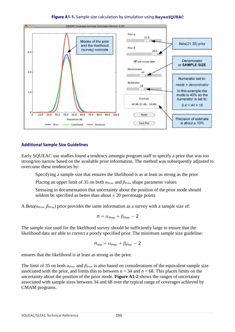
arly QU C use studies found a tendency amongst program staff to specify a prior that was too strong o n ow b d on e av abl ior orm n m d s tl djus d

er e t es en ci by:pecifying a sample size that ensures the likelihood is as at least as strong as the prioracing an upper limit of 35 on both αPrior and βPrior shape parameter valuesressing in documentation that uncertainty about the position of the prior mode should

eldom be specified as better than about ± 20 percentage points

Beta(αPrior, βPrior) prior provid the m f on a su y with a sample size of:

he m si sed r like ho urve sh be ffi ntly large to ensure that the elihood data are able to correct a poorly specified prior. The minimum sample size guideline:

sur ha li od t as s n th

e limit of 35 on both αPrior and βPrior is also based on consid io of e va sa le e associated with the prior, and limits this to between n = 34 and n = 68. This places limits on the

certainty about the position of the prior mode. Figure A1-2 shows the ranges of uncertainty associated with sample sizes between 34 and 68 over the typical range of coverages achieved by

MAM programs.


Figure A1-1. Sample size calculation by simulation using BayesSQUEAC

E S EA/to arr ase th ail e pr inf atio . The etho was ubsequen y a te to

ov com h e t den es SPlSts

A es sa e in ormati as rve


T sa ple ze u fo the li od s y ould su cielik


en es t t the keliho is a least tro g as e prior.

Th erat ns the qui lent mp siz

un

C

Additional Sample Size Guidelines

Figure A1-2. Uncertainty/precision associated with sample sizes between 34 and 68 over the typical range of coverages achieved by CMAM programs

The stress that uncertainty about the position of the prior mode should seldom be specified as better than about ± 20 percentage points means that a sample size for the likelihood survey larger than about:

7nlikelihood =⌈ 7 14α

9 Prior + β9 Prior − 9 ⌉

is required to estimate coverage with a precision of ± 15 percentage points or better and a sample size for the likelihood survey larger than about:

nlikelihood = ⌈ 3αPrior + 3βPrior − 6 ⌉

is required to estimate coverage with a precision of ± 10 percentage points or better.

The guidelines related to sample size help to ensure a reasonably large sample size for the likelihood survey and help prevent posterior estimates being dominated by an overly strong prior.

Additional sample size guidelines apply when using small values of αPrior and βPrior and analysing data by hand. These are discussed in the following section on ‘Formula for the 95% Credible Interval on the Posterior Mode’.


Formula for the 95% Credible Interval on the Posterior Mode

The formula given to calculate the 95% credible interval on the posterior mode:

× βode √ α

95%CI = m ± 1.96 × Posterior Posterior

(α 2Posterior + βPosterior) × (αPosterior + βposterior + 1)

returns an approximate equal-tailed 95% credible interval on the posterior mode rather than an exact highest posterior density (HPD) 95% credible interval on the posterior mode. The term:

αPosterior × βPosterior

(αPosterior +β 2Posterior) × (αPosterior + βposterior + 1)

is the variance of Beta(αPosterior, βPosterior), and 1.96 closely approximates the standard normal deviate for the 97.5th percentile point of the standard normal distribution. This approach is analogous to using the normal approximation when calculating an approximate 95% confidence interval on a binomial proportion. This is considered safe when:

np > 5 and n – np > 5

where:

n = α Posterior + β Posterior – 2

p = posterior mode

Problems occur at extremely low and extremely high values of p or when very small effective sample sizes (n) are used. The purpose of the guideline:


is to ensure that a safe effective sample size (n) is used for values of p between about 17% and 83%. Most CMAM programs achieve levels of coverage within this range.

A normal approximation will only be safe when the Beta(αPosterior, βPosterior) distribution can be approximated by a normal distribution. A Beta(α, β) distribution can be approximated by a normal distribution when α and β are sufficiently large such that:

α+ 1 β + 1≈ 1 and ≈ 1α− 1 β − 1

A common rule-of-thumb is that a normal approximation is probably safe to use when both α and β are greater than or equal to 6 and that the normal approximation is safe to use when both α and β are greater than or equal to 10. For example, Figure A1-3 shows how well the normal approximation fits Beta(α, β) distributions with two different modes and different values of α and β. The purpose of the guideline:

⌊ αPrior + mode × nLikelihood ⌋ ≥ 10 and ⌊ βprior + nLikelihood − mode ×nLikelihood ⌋ ≥ 10

is to ensure that the normal approximation returns reasonably accurate results.


Figure A1-3. Normal approximation to Beta(α, β) distributions with two different modes and different values of α and β


The 95% Credible Interval on the Posterior Mode in BayesSQUEAC

BayesSQUEAC estimates the mode of the posterior from αPrior and βPrior using the standard formula:

αmode = Posterior − 1

αPosterior +βPosterior − 2

The 95% credible interval is found by a bootstrap aggregation (‘bagging’) method:

1. 100 sets of 100 replicates drawn at random from the Beta(αPosterior, βPosterior) distribution are generated.

2. The 0.025 and 0.975 quantiles of each of the 100 sets of replicates are found.

3. The means of the sets of 0.025 and 0.975 quantiles from Step 2 are calculated.

The bagging algorithm is faster and more accurate than a simple bootstrap algorithm. Using 10,000 (i.e., 100 sets of 100) replicates the bagging algorithm provides an ‘approximately exact’ equal-tailed 95% credible interval.

BayesSQUEAC does not use a normal approximation to Beta(αPosterior, βPosterior). This means that the guidelines:


and:

⌊ αPrior + mode × nLikelihood ⌋ ≥ 10 and ⌊ βprior + nLikelihood − mode ×nLikelihood ⌋ ≥ 10

need not be applied if data are to be analysed using BayesSQUEAC.

Formulas for Finding Suitable Values for αPrior and βPrior

The formulas used for finding suitable values for αPrior and βPrior are:



μ ×αPrior = μ ×( (1 − μ)

σ2 − 1)μ ×

βPrior =(1 −μ) ×( (1 − μ)σ 2 − 1)

The formulas for μ and σ are taken from the three-point estimation approach to task-duration modelling used in the Project Evaluation and Review Technique (PERT) and Critical Path Method (CPM) project management techniques.


Distributions that can be defined by the three points of mode, minimum, and maximum values are useful in PERT and CPM because task completion times are commonly specified as the most likely case (mode), the worst case (maximum), and the best case (minimum). The reason that the three-point estimation approach is used in PERT and CPM is because it is quick, easy, accurate, reliable, and easy to teach.

The approach used in PERT and CPM is:

1. Make informed guesses of the mode, minimum, and maximum.

2. Estimate the mean (µ) and the standard deviation (σ) of a beta distribution using the mode, minimum and maximum:



3. Find suitable values for the α and β shape parameters of the required beta distribution using the standard formulas:

μ ×αPrior = μ ×( (1 − μ)

σ2 − 1)μ ×

βPrior =(1 −μ) ×( (1 − μ)σ 2 − 1)

The same process is used in SQUEAC. The method is approximate. This is acceptable in Bayesian analysis because a prior is never exact.

Simplified LQAS and the Rule-of-Thumb Formula

The simplified LQAS method was developed to meet the need for SQUEAC and SLEAC assessments to be conducted without using computers. The method is ‘simplified’ because it does not bother the user with such matters as the selection of appropriate probability distributions, specification of lower and upper triage thresholds, or the specification of provider and consumer errors. Unlike conventional sequential methods, the simplified LQAS method starts with a given sample size and works from that. The rule-of-thumb formula provides a ‘rough and ready’ way of creating an LQAS sampling plan.


pl the - b m o sta w s le giv

on t LQ wo u h ib f prob mis drawn without replacement from a (usually) small population of SAM cases. Using a reverse

pergeometric LQAS calculator designed to find the best sampling plan for a given sample size:

pe u 0Th c

wer value : 0.40mpl ze

he ram Us fau al

ca n 5, i sam a retu d ru hu rm

rule-of-thumb formula will return the same or very similar values for a given sample size and ng point as conventional LQAS using the binomial or hypergeometric distribution.

simplified LQAS method does not quantify error, but there are good reasons to believe that errors will be small. The population size is small and the active and adaptive case-finding metho

plied correctly) yield a large sampling proportion. Assuming the case-finding method has an 80% exhaustivity (i.e., the method finds 80% of all SAM cases in the area sampled) and continuing with

= 50%, n = 11 example, then the population size would be:


Ap ying rule of-thum for ula t 50% ndard (p) ith a amp size of 11 es:

11d = ⌊ 2 ⌋= ⌊5.5⌋ = 5 which is the same as d = ⌊ p

11 ×100 ⌋= ⌊ 50

11 ×100 ⌋= ⌊5.5⌋ = 5

C ven ional AS uld se t e hypergeometric distr ution or this lem because the sa ple

hy

http://www.brixtonhealth.com/hyperLQAS.findD.html

and specifying:

Up r val e : 0.6 ese spe ify a 50% swing point

LoSa e si : 11

Ot r pa eters : e de lt v ues

the calculator returns:

The lculator retur s d = which s the e v lue as rne by the le-of-t mb fo ula.

Theswi

The d (if

ap

the p

1Population size = ⌈11 ×

0.8 ⌉= 14

ng eve hyp et Q culat spe

per value : 0.60 These specify a 50% swing point

wer value : 0.40mple size : 11

pulation size : 14

he errors associated with the decision rule found using the rule-of-thumb formula are reasonably all. It is important to realize that error in small-area surveys is more complicated than classifying

coverage without a prior hypothesis about a proportion. SQUEAC uses a two-stage model that aims confirm or deny a prior hypothesis regarding coverage. In such circumstances, the practical

meaning of errors (i.e., the positive and negative predictive values) are very different from the naive QAS case. This is analogous to a two-stage screening-test model.

g s ci s Q me ho is s to ur erro er er by altering the rounding rule used in the rule-of-thumb formula:

• rule-of-thumb formula used in the SQ um ation employs the rounding down (floor) rule. For measures of success (e.g., coverage), this favours the provider. For measures

ailure (e.g., defaulting), this favours the consumer.

• ounding to the nearest whole number favours neither consumer nor the provider.

ou up vou c r fo s of s ess , c ge d fa u ovid or sur of f re , de lti


Usi the r rse ergeom ric L AS cal or and cifying:

UpLoSa

PoOther parameters : Use default values

the calculator returns:

Tsm

to

L

Althou h error i not spe fied in the implified L AS t d, it po sible favo one r ovanoth

Rounding rule

Round down (floor) Round to nearest whole number Round up (ceiling)

pd = n ×⌊ ⌋100

pd =∥n ×

100∥ pd = n ×⌈ ⌉100

Different rounding rules favour different errors:

The UEAC doc ent

of f

R

• R nding fa rs the onsume r measure ucc (e.g. overa ) an vo rs thepr er f mea es ailu (e.g. fau ng).

To avoid confusion, the SQUEAC documentation presents a single rounding rule. The rounding down (floor) rule was chosen for simplicity. More advanced users of the simplified LQAS method might like to use rounding up for measures of success (e.g., coverage) and rounding down for measures of failure (e.g., defaulting). Such a strategy will always favours the consumer.

Modelling Coverage Using the Binomial Distribution

The use of the beta-binomial conjugate analysis assumes that it is safe to model likelihood survey data using the binomial distribution. The binomial model assumes that the likelihood survey samples n observations from a population of size N with replacement. The likelihood survey violates this assumption by sampling without replacement. This violation is not usually considered to be problematic if the sampling proportion:

nSampling proportion =

N

remains small. The most frequently used rule-of-thumb is that it is safe to use the binomial model when:

n ≤ N × 0.1

At this sampling proportion (10%), under-dispersion (the ‘finite population correction’) is just below 0.95. With a sampling proportion of 20%, it is just below 0.90.

The likelihood survey estimates coverage in the program area using a sample of current and recovering SAM cases in the program area found in a sample of villages in the program area. Experience with CSAS, SQUEAC, and SLEAC indicates that it is rare for more than about 10% or 15% of villages to be sampled to achieve the required sample size. The proportion of villages sampled may be used as a proxy for the sampling proportion and will usually overestimate the true sampling proportion because villages are not selected using population proportional sampling.

Data arising from a sample drawn from a small population without replacement should be modelled using the hypergeometric distribution. Working with the hypergeometric distribution requires good estimates of the population size (i.e., the total number of current and recovering SAM cases in the program area). It is uncommon to have good estimates of the population size with which to calculate exact hypergeometric probabilities. The binomial model does not require this information. SQUEAC likelihood surveys, therefore, use the binomial approximation for the hypergeometric. The nature of the error associated with the use of the binomial distribution is related to the relative under-dispersion of the hypergeometric compared to the binomial. The estimate of mode (i.e., the point estimate of coverage) is not affected. Use of the binomial model results in the use of a slightly larger sample size and produces slightly wider credible intervals than if the hypergeometric model were used.

It is important to note that the beta-binomial conjugate analysis is convenient in the sense that the method of analysis is relatively simple. This informed the choice of method because of the need to provide methods that could be performed without using a computer. It is not feasible to use the hypergeometric distribution without using a computer. Software to perform the required analysis (e.g., winBUGS, openBUGS, JAGS) is designed to be used by professional statisticians and is probably too complicated for the majority of the SQUEAC user group.


The Use of n = 40 as the Standard Sample Size for SLEAC

The use of n = 40 as the standard sample size for SLEAC surveys was informed by the need to provide accurate and reliable classification of coverage as being above or below Sphere minimum standards using small sample sizes. This sample size was selected after computer-based simulation of the two-class and three-class simplified LQAS methods. Simulation parameters were:

Parameter Values

Sample sizes 20, 25, 30, 35, 40, 45, 50, 55, 60, 65, 70, 75, 80Coverage proportion 0%, 1%, 2%, …, 98%, 99%, 100%Simulated surveys 1,000 simulated surveys at each coverage proportionPopulation size 400

ThresholdsTwo classes

50% (Sphere rural)70% (Sphere urban/camp)

Three classes20%/50%30%/70%

The population size of 400 is derived from the following assumptions:

• The thes

largest service delivery unit for which coverage will be classified is a health district and e are seldom larger than 100,000 total population.

• Approximately 20% of the population are aged between 6 and 59 months.

• A SAM prevalence of 2%.

These parameters yielded a population size of:

20 2Population Size = 100,000 × × = 400

100 100

High parameter values were selected to maximise the population size.

The performance of the method was assessed by examination of operating characteristic curves and probability of classification plots.

A minimum sample size of n = 40 was selected as appropriate for SLEAC surveys. Figure A1-4 shows the operating characteristic plots and probability of classification plots found for n = 40. The curves are steep and there are no gross misclassifications. At lower prevalences or in smaller populations, the method will perform better than indicated by the operating characteristic curves and probability of classification plots shown in Figure A1-4 as the sampling proportion increases.


Figure A1-4. Operating characteristic and probability of classification plots found from simulations of two-class and three-class SLEAC methods with n = 40

Two-class, n = 40, d = 20 (50%: Sphere rural) Two-class, = 40, = 28 (70%: Sphere urban/camp)

Three-class, = 40, 1 d2 n d1 = 12, = 28 (30%/70%)

Smoothing Time-Series Data Using Moving Averages

SQUEAC requires you to analyse a variety of time-series, such as admissions and exits over time. This type of data usually requires smoothing before being plotted using line charts.

You can smooth data using the charting functions in spreadsheet applications. If you do this, make sure that you use a smoothing function that is suited to time-series data. These will usually be called something like ‘moving average’ or ‘running average’.

Do not worry if your spreadsheet package does not provide moving average functions. It is easy to program these functions yourself. Figure A1-5 shows how to program a spreadsheet for three different types of moving average and the effect that these have on a time-series.


Figure A1-5. Programming a spreadsheet for three different moving averages with a span of three successive data points

A

1

B

2

3

4

5

6

7

8

9

10

11

12

13

14

=MEDIAN(A2:A3)

=MEDIAN(A2:A4)

=MEDIAN(A3:A5)

=MEDIAN(A4:A6)

=MEDIAN(A5:A7)

=MEDIAN(A6:A8)

=MEDIAN(A7:A9)

=MEDIAN(A8:A10)

=MEDIAN(A9:A11)

=MEDIAN(A10:A12)

=MEDIAN(A11:A13)

=MEDIAN(A12:A14)

=MEDIAN(A13:A14)

98

112

122

83

104

125

112

125

121

100

107

147

127

Raw M3

A

1

B

2

3

4

5

6

7

8

9

10

11

12

13

14

98

112

122

83

104

125

112

125

121

100

107

147

127

Raw M3

105

112

112

104

104

112

125

121

121

107

107

127

135

A

1

B

2

3

4

5

6

7

8

9

10

11

12

13

14

98

112

122

83

104

125

112

125

121

100

107

147

127

Raw A3

A

1

B

2

3

4

5

6

7

8

9

10

11

12

13

14

98

112

122

83

104

125

112

125

121

100

107

147

127

Raw A3

105

111

106

103

104

114

121

119

115

109

116

125

135

=AVERAGE(A2:A3)

=AVERAGE(A2:A4)

=AVERAGE(A3:A5)

=AVERAGE(A4:A6)

=AVERAGE(A5:A7)

=AVERAGE(A6:A8)

=AVERAGE(A7:A9)

=AVERAGE(A8:A10)

=AVERAGE(A9:A11)

=AVERAGE(A10:A12)

=AVERAGE(A11:A13)

=AVERAGE(A12:A14)

=AVERAGE(A13:A14)

A

1

C

2

3

4

5

6

7

8

9

10

11

12

13

14

98

112

122

83

104

125

112

125

121

100

107

147

127

Raw A3

B

M3

=MEDIAN(A2:A3)

=MEDIAN(A2:A4)

=MEDIAN(A3:A5)

=MEDIAN(A4:A6)

=MEDIAN(A5:A7)

=MEDIAN(A6:A8)

=MEDIAN(A7:A9)

=MEDIAN(A8:A10)

=MEDIAN(A9:A11)

=MEDIAN(A10:A12)

=MEDIAN(A11:A13)

=MEDIAN(A12:A14)

=MEDIAN(A13:A14)

=AVERAGE(B2:B3)

=AVERAGE(B2:B4)

=AVERAGE(B3:B5)

=AVERAGE(B4:B6)

=AVERAGE(B5:B7)

=AVERAGE(B6:B8)

=AVERAGE(B7:B9)

=AVERAGE(B8:B10)

=AVERAGE(B9:B11)

=AVERAGE(B10:B12)

=AVERAGE(B11:B13)

=AVERAGE(B12:B14)

=AVERAGE(B13:B14)

A

1

B

2

3

4

5

6

7

8

9

10

11

12

13

14

98

112

122

83

104

125

112

125

121

100

107

147

127

Raw M3

105

112

112

104

104

112

125

121

121

107

107

127

135

C

A3

109

110

109

107

107

114

119

122

116

112

114

123

131

Running medians-of-three (M3)

Running averages-of-three (A3)

Running medians-of-three followed by running averages-of-three (M3A3)


Moving averages can be applied several times. This involves applying a smoothing method to previously smoothed data, as is done with the M3A3 smoother shown in Figure A1-5. With the M3A3 smoother, the data are smoothed by taking the medians of sets of three successive data points (M3). The results are then smoothed by taking the arithmetic means of sets of three successive smoothed data points (A3). The more times you apply a moving average, the more smoothing is applied to the data.

A time-series can be thought of as a combination of random (irregular or ‘noise’), seasonal, and trend components. Judicious application of smoothing techniques, such as moving averages, hides some of these components and helps uncover other components of the time-series:

• Smoothing using moving averages of short spans (i.e., of just a few successive data points) will tend to hide the random ‘noise’ component and help reveal the seasonal and trend components of the time-series.

• Smoothing using moving averages of longer spans (i.e., of enough data points to cover an entire seasonal cycle) will tend to hide both the random ‘noise’ and seasonal components and help reveal the trend component of the time-series.

Figure A1-6 shows the effect of smoothing 6 years of monthly data using smoother spans of 3 to hide the random (irregular or ‘noise’) component and smoother spans of 13 to hide both the random (irregular or ‘noise’) and seasonal components.

Figure A1-6. Effects of moving average smoothers of spans 3 (M3A3) and 13 (M13A13) on 6 years of monthly admissions data


Mid-yearpeaks

1 year 4 years

Seasonalcycle No simple trend, but a possible long-term cycle

Noise + Season + TrendSeason + Trend

Trend

It is also possible to find the seasonal component alone by subtracting the trend component (i.e., the data smoothed using M13A13) from the combined season and trend components (i.e., the data smoothed using M3A3). This is shown in Figure A1-7.

Figure A1-7. Seasonal component of 6 years of monthly admissions data found by subtracting data smoothed using M13A13 from data smoothed using M3A3


Appendix 2. Working with Formulas

Formulas are devices that precisely describe calculations. A number of mathematical formulas are presented in this document. This appendix contains some basic information to help you work with these formulas.

Parts of Formulas

Formulas are made up from a number of basic parts. These are:Sides. A formula usually has two sides. One side, usually the left-hand side

side (RH(LHS)S), pr

, is ecise

reserved for the result of the calculation. The other side, usually the right-hand ly describes the data and calculations required to find the result. The two sides are separated by an assignment (=) operator. For example:

stants. Constants are numbers that are the same for all contexts. They are shown in formulas num n this formula:

number 100 is a constant. The value 100 is used whenever this formula is used. It is a nstant because it does not change.

ables. Variables are placeholders for values that change (i.e., are different in different exts). You have to provide the appropriate values for each of the variables when you use a ula this formula:

e letters n and p are variables. The letters or names given to variables frequently indicate the type of data that is required to perform the calculation and the type of data that is produced as the

ult of the calculation. In the example formula, d is a number that is used to make a decision (i.e., d for ‘decision’), n is used to indicate a sample size (i.e., n for ‘number’) and p is used to

dicate a percentage (i.e., p for ‘percentage’). The use of variables allows formulas to present calculations and methods in a way that enables the same formula to be used in different contexts

th different data.

ators. Operators specify the operations that are performed on the constants and variables in ormul T era ed in SQUEAC and SLEAC formulas are shown in Table A2-1. This mu

s th flo o n tip d op . T rat re d c nts and variables in a specific order called the order of precedence.


LHS

(Result) Assignment operator

pd = ⌊n ×

100 ⌋

RHS

(Calculation)

Conas bers. I

pd =⌊n×

100 ⌋the co

Varicontform . In

d = ⌊ pn ×

100 ⌋th

res

in

wi

Opera f a. he op tors usfor la:

d = ⌊ pn ×

100 ⌋use e ‘ or’ (r und dow ), mul ly, an divide erators he ope ors a applie to the onsta

Table A2-1. Operators used in SQUEAC and SLEAC formulas

Symbol Meaning Example Notes

x = y Assignment d =⌊n × p100 ⌋ Separates the result and the calculations in a formula.

+ Add 4 + 2 = 6 Simple addition

− Subtract 4 − 2 = 2Also used to indicated negation as in:

−2 = 0 − 2 or ‘minus 2’ or ‘negative 2’

× Multiply 4 × 2 = 8

A ‘dot-product’ operator may be used in formulas. The operator may also be missing in formulas. For example:

a × b = a⋅b = ab

÷ Divide 4 ÷ 2 = 2 or 42 = 2

The ‘over’ operator is useful for grouping expressions. For example:

2 + 23 − 1 =(2 + 2) ÷ (3 − 1) = 4 ÷ 2 = 2

± Add and subtract 6 ± 3 = { 3, 9 }

This operator return two values. It is used when calculating credible limits. For example:

95%CI = mode ± 1.96×√ α×β(α +β)2×(α + β +1)

∑ Sum a series ofnumbers ∑ { 1, 2, 3 } = 1 + 2 + 3 = 6

Used when calculating a mean (average) value. If, for example:

x = { 6, 9, 7 }

Then the mean value is:

Mean =∑ x3

= 6 + 9 + 73

= 223

= 7.33

⌊ x ⌋ Round x towardszero (floor) ⌊ 2.7 ⌋ = 2

Used when finding classification thresholds for simplified LQAS sampling plans. For example:

d =⌊11 × 70100 ⌋= ⌊ 11 × 0.7 ⌋ = ⌊ 7.7 ⌋ = 7

Rounding operators act like brackets grouping expressions and altering the normal order of precedence.

⌈ x ⌉ Round x away fromzero (ceiling) ⌈ 2.7 ⌉ = 3

Use in sample size calculations. For example:

n =⌈ 41

600 × 20100

× 1100 ⌉= ⌈ 34.17 ⌉= 35

Rounding operators act like brackets grouping expressions and altering the normal order of precedence.

∥ x ∥ Round to nearestwhole number ∥2.3∥= 2 and ∥2.7∥= 3

May be used when finding classification thresholds for simplified LQAS sampling plans as explained in Appendix 1. Rounding operators act like brackets grouping expressions and altering the normal order of precedence.

( x ) Group expression 3 × (2 + 1) = 3 × 3 = 9Brackets alter the order of precedence. The calculations in brackets are completed before all other calculations.

[ x ] Group expression 3 × [2 + 1] = 3 × 3 = 9

As above. Square brackets are used to help avoid confusion in long or complicated calculations. For example:

Coverage =∑[( N∑ N )× c

n ]x y Power or

exponentiation 32 = 3 × 3 = 9Exponentiation and roots are the same underlying operation as with, for example:

√x = x 0.5√x Square root √ 9 = 3


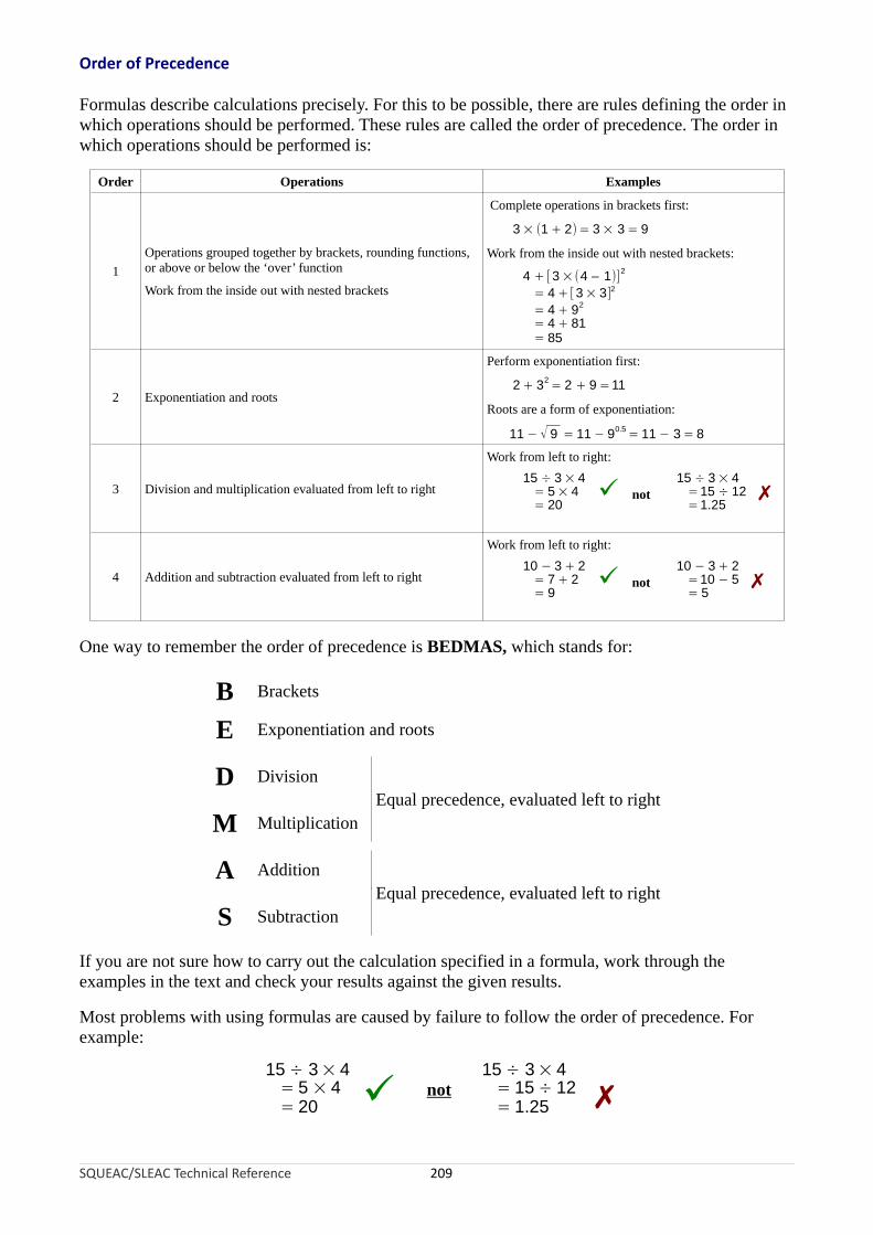
Order of Precedence

Formulas describe calculations precisely. For this to be possible, there are rules defining the order in which operations should be performed. These rules are called the order of precedence. The order in which operations should be performed is:

Order Operations Examples

Complete operations in brackets first:

3 × (1 + 2) = 3 × 3 = 9

1Operations grouped together by brackets, rounding functions, or above or below the ‘over’ function

Work from the inside out with nested brackets

Work from the inside out with nested brackets:

4 +[3 ×(4 – 1)]2

= 4 +[3 × 3]2 = 4 + 92

= 4 + 81= 85

2 Exponentiation and roots

Perform exponentiation first:

2 + 32 = 2 + 9 =11

Roots are a form of exponentiation:

11 − 90.511 − √ 9 = = 11 − 3 = 8

3 Division and multiplication evaluated from left to right

Work from left to right:15 ÷ 3 × 4

= 5 × 4 ✓ not = 20

15 ÷ 3 × 4=15 ÷ 12=1.25

✗

4 Addition and subtraction evaluated from left to right

Work from left to right:10 − 3 + 2

= 7 + 2 ✓ not = 9

10 − 3 + 2=10 − 5= 5

✗

One way to remember the order of precedence is BEDMAS, which stands for:

B Brackets

E Exponentiation and roots

D DivisionEqual precedence, evaluated left to right

M Multiplication

A AdditionEqual precedence, evaluated left to right

S Subtraction

If you are not sure how to carry out the calculation specified in a formula, work through the examples in the text and check your results against the given results.

Most problems with using formulas are caused by failure to follow the order of precedence. For example:


15 ÷ 3 × 4 15 ÷ 3 × 4= 5 × 4 = 15 ÷ 12= 20 ✓ not

= 1.25 ✗

Percentages and Proportions

Many formulas in this document require you to use proportions or return a result that is expressed as a proportion. Conversions between proportions and percentages are straightforward:

PercentageProportion = and Percentage = Proportion × 100

100

Chains of Formulas

Some formulas are chained together. This is done to simplify calculations, with the results of one formula being used in subsequent formulas. For example:



μ ×αPrior = μ ×( (1 − μ)

σ2 − 1)μ ×

βPrior =(1 −μ) ×( (1 − μ)σ 2 − 1)

In this set of formulas, the results that we are interested in are αPrior and βPrior, which are calculated using μ and σ, which are calculated from the variables called minimum, mode, and maximum.

It is possible, for example, to calculate βPrior directly using minimum, mode, and maximum as:

[minimum+4×mode+maximum minimum+4×mode+maximum× 1−β = ( minimum+4×mode+maximum 6 ( 6 )

Prior 1 − )× − 16 (maximum−minimum )

2

6]

but the calculation would be complicated, repetitious, and prone to error.

If in Doubt …

If you are not sure how to carry out the calculation specified in a formula, work through the examples given in the text and check your results against the results given in the text. Most problems are caused by failure to follow the order of precedence. Another common problem is using percentages when proportions are required. Most formulas in the text require you to use proportions and return proportions.


Appendix 3. Glossary of terms

Accuracy. The degree of closeness of a measurement of a quantity to the measured quantity’s true value. See precision.

Active and adaptive case-finding. A type of sampling used in SQUEAC small-area surveys, SQUEAC likelihood surveys, and SLEAC surveys. This type of sampling searches actively for cases of SAM with the intention of finding all (or nearly all) cases of SAM in sampled communities. This type of sampling is also known as ‘snowball sampling’, ‘optimally biased sampling’, or ‘chain-referral sampling’. See sample, sampling.

Active case. See current case.

Acute malnutrition. A form of undernutrition caused by infection and/or a decrease in food intake or uptake resulting in rapid weight loss (wasting) or bilateral pitting oedema. Acute malnutrition is defined by the presence of bilateral pitting oedema or wasting (low MUAC or low weight-for-height). See bilateral pitting oedema, global acute malnutrition, kwashiorkor, mid-upper arm circumference, moderate acute malnutrition, severe acute malnutrition, visible severe wasting.

Admission criteria. Rules describing individuals that are eligible for admission to a program. Also known as the program’s ‘case definition’. In CMAM programs, the admission criteria is usually ‘MUAC < 115 mm or bilateral pitting oedema or visible severe wasting in a child aged between 6 months and 5 years’. Some CMAM programs may also use weight-for-height for admission. See bilateral pitting oedema, case definition, discharge criteria, visible severe wasting.

Aetiology. The cause, origin, or reason for something (usually of a disease or abnormal condition).

Anthropometric criteria. Admission or discharge criteria using anthropometry (usually MUAC). See admission criteria, anthropometry, discharge criteria, mid-upper arm circumference.

Anthropometry. Measurement of the proportion, size, or weight of the human body or a human body part. Anthropometric measurements are used to assess the nutritional status of individuals and population groups, and as admission and discharge criteria for nutrition support programs. CMAM programs use MUAC (for screening/case-finding, admission, monitoring response to treatment, discharge) and weight (for monitoring response to treatment and discharge). Some CMAM programs may also use weight-for-height for admission. See case-finding, mid-upper arm circumference, screening.

Areal. A description of one of more areas. In SLEAC and SQUEAC, for example, quadrats may be described as ‘areal sampling units’. See centric systematic area sampling, quadrat, systematic area sampling.

ARI. Acronym for ‘acute respiratory infection’. The acronym ARTI (for ‘acute respiratory tract infection’) is also in common use.

Attack phase. A phase in the program cycle during which coverage is increased. The term is usually applied to the first few months of program activity, but may be used to describe the period following program reforms designed to improve coverage.

Bar chart. A chart drawn using rectangular bars with lengths proportional to the values that they represent. The bars may be drawn vertically or horizontally. See Pareto chart.


Barrier. Anything that restrains, obstructs, or delays access to a program or restrains coverage. See booster.

Bayesian. The interpretation of probability as a measure of confidence (or belief) that something is true. In Bayesian inference, belief is modified as fresh evidence is observed. At each step, the initial belief is called the ‘prior’, the fresh evidence is called the ‘likelihood’, and the modified belief is called the ‘posterior’. See frequentist, likelihood, posterior, prior.

Beneficiary record card. A card recording beneficiary data, including (but not limited to) identifying, locating, demographic, clinical, and anthropometric data. The card is used to record all relevant information about a beneficiary and the treatment episode. Beneficiary record cards usually follow the design developed by Valid International for use in CTC programs.

Best practice. A method or technique that has consistently shown results superior to those achieved by other means. In addition, a ‘best’ practice can evolve to become better as improvements are discovered. SQUEAC uses the clinical audit approach to evolve best practice (i.e., the practices that maximise program coverage). See clinical audit.

Beta-binomial conjugate analysis. In Bayesian inference, a type of conjugate analysis in which the prior and posterior are modelled using the beta distribution and the likelihood is modelled using the binomial distribution. See beta distribution, binomial distribution, conjugate analysis, likelihood, posterior, prior.

Beta distribution. A family of probability distributions defined on the interval [0, 1] parameterised by two positive shape parameters denoted α and β. The beta distribution is suited to the statistical modelling of proportions. SQUEAC uses the beta distribution to model the coverage proportion.

Bilateral pitting oedema. A sign of SAM caused by an accumulation of fluid in the interstitial tissue spaces (the areas surrounding the body’s cells and blood vessels). See acute malnutrition, kwashiorkor, severe acute malnutrition.

Binary variable. A variable that can take one of two complementary values. In SQUEAC, this is usually the coverage status of a SAM case (i.e., the SAM case is either ‘covered’ or ‘not covered’). See variable.

Binomial distribution. A probability distribution suited to the statistical modelling of proportions of a binary variable. SQUEAC uses the binomial distribution to model coverage in likelihood surveys. See binary variable, likelihood, variable.

Booster. Anything that encourages or enables access to a program or leads to an increase in coverage. See barrier.

Branching hierarchy. A way of organising findings in a mind-map. SQUEAC investigations tend to use mind-maps organised using a Central Theme → Data Source/Method → Individual Findings hierarchy. See mind-map.

Case, active. See current case.

Case, current. See current case.

Case, recovering. See recovering case.


Case definition. The method by which cases of SAM are defined for purposes of admission to a program. The term may apply to other situations, such as defining defaulters, defining failure to respond to treatment, or defining when a beneficiary has recovered and may be discharged from a program. See admission criteria, discharge criteria.

Case-finding. Activities aimed at finding and recruiting current cases. Effective CTC/CMAM programs usually employ many case-finding strategies, including screening children attending health centres, screening children in the community by program staff or CHWs, screening children attending vaccination sites, screening children attending growth monitoring programs, screening children by CBVs, and referring cases to the program by carers of program beneficiaries. The use of MUAC facilitates the use of diverse case-finding strategies. See community-based volunteer, community health worker, current case, mid-upper arm circumference, screening.

Case history. A detailed account of the facts affecting the development or condition of a person (or group) under treatment or study.

Catchment area. The area served by a service delivery unit such as a health centre or health post. See service delivery unit.

CBV. See community-based volunteer.

Census. The procedure of systematically acquiring and recording information about all members of a given population or household. See census sample.

Census sample. A sample that is designed to include all (or nearly all) members of a given population. SQUEAC uses census samples in small-area surveys and in likelihood surveys through the use of active and adaptive case-finding and house-to-house/door-to-door sampling. See active and adaptive case-finding, sample, sampling.

Centric systematic area sampling (CSAS). A way of taking a spatially stratified/spatially representative sample that involves drawing a grid of equally sized squares (‘quadrats’) over the area to be sampled and sampling the community or communities located closest to the centre of each square. See sample, sampling, spatial, systematic area sampling, systematic sampling.

CHW. See community health worker.

Clinic workload returns. Routine statistics on clinic activities usually including (but not limited to) counts of cases of specific diseases seen at a clinic in a reporting period.

Clinical audit. A quality improvement and monitoring method that seeks to improve service delivery through systematic review against specific criteria and standards and the implementation of change. SQUEAC uses clinical audit to evolve best practice. See best practice.

Clinical trial. A carefully controlled study conducted to test the effectiveness and safety of new drugs, medical products, protocols, or techniques

CMAM. See Community-Based Management of Acute Malnutrition.

Community-Based Management of Acute Malnutrition (CMAM). Refers to a program delivering therapeutic feeding to the majority of cases of severe wasting as outpatients. Effective CMAM programs include community outreach, mobilisation, and sensitisation activities to help ensure early detection, referral, and recruitment of cases and the follow-up of cases in the community. See Integrated Community-Based Management of Acute Malnutrition, Community-Based Therapeutic Care, mobilisation, outpatient, outreach, sensitisation.


Community-Based Therapeutic Care (CTC). Usually refers to NGO-run programs delivering therapeutic feeding to the majority of cases of severe wasting as outpatients in natural and civil emergencies. Effective CTC programs include community outreach, mobilisation, and sensitisation activities to help ensure early detection, referral, and recruitment of cases and the follow-up of cases in the community. See Community-Based Management of Acute Malnutrition, Integrated Community-Based Management of Acute Malnutrition, mobilisation, outpatient, outreach, sensitisation.

Community-based volunteer (CBV). A member of the community who assists with program activities (usually community mobilisation and case-finding and referral). CBVs typically do unpaid work on a ‘little and often’ basis. A CBV can receive an incentive (e.g., for attending training or per-referral), but no regular remuneration. Effective CTC and CMAM programs usually recruit and involve very many CBVs to assist with program activities. See case-finding, community health worker, mobilisation.

Community health worker (CHW). A member of a community who provides basic health and medical care to the community. CHWs may deliver CMAM services, such as community-based screening and referral, facility-based screening and diagnosis, and treatment. See community-based volunteer.

Community mobilisation. See mobilisation.

Community sensitisation. See sensitisation.

Compliance. The degree of constancy and accuracy with which a prescribed regimen (treatment protocol) is followed. The term is usually applied in the negative sense (i.e., non-compliance or poor compliance). The term may be applied to beneficiaries when, for example, RUTF is shared within the household, clinic visits are missed, or drugs are not given/taken. The term may be applied to a program or to program staff when, for example, the full CMAM protocol is not delivered.

Concept map. A diagram showing the relationships between findings. A graphical tool for organising and representing knowledge. Findings are represented as boxes or circles and connected using labeled arrows. The relationship between findings may be expressed using such phrases as ‘gives rise to’, ‘contributes to’, ‘results in’, and ‘is required by’. See mind-map.

Confidence interval. In frequentist inference, an interval used to indicate the reliability (precision) of an estimate. See credible interval, frequentist.

Confidence limits. Upper and lower end-points of a confidence interval. See confidence interval.

Conjugate analysis. In Bayesian inference, a prior can be used that produces a posterior distribution of the same form as the prior distribution. Such a prior is called a ‘conjugate prior’. When a conjugate prior is used, the prior to posterior Bayesian analysis is called a ‘conjugate analysis’. SQUEAC uses beta-binomial conjugate analysis in which a beta-distributed prior is modified by a binomially distributed likelihood, resulting in a beta-distributed posterior. See beta-binomial conjugate analysis, beta distribution, binomial distribution, likelihood, posterior, prior.

Consumer. A synonym for beneficiary. A term used in LQAS. See consumer probability of error, Lot Quality Assurance Sampling, provider, provider probability of error.

Consumer probability of error (CPE). The risk that an investigation will conclude that coverage is high when it is (in fact) low. Also known as ‘consumer risk’. See Lot Quality Assurance Sampling, provider probability of error.


Coverage. The proportion of all people needing or eligible to receive a service that actually receive that service. Also known as ‘treatment coverage’.

Coverage failure. An event or circumstance that results in people that need a service or are eligible for a service failing to receive that service. Examples of coverage failures are defaulters, DNA referrals, late admissions, and lack of proximity of services to the beneficiary population.

CPE. See consumer probability of error.

CPM. See Critical Path Method, Program Evaluation and Review Technique.

Credible interval. In Bayesian inference, a way of summarising the posterior distribution that gives an interval within which most (usually 95%) of the posterior distribution lies. A credible interval predicts that the true value of a parameter has a particular probability (usually 95%) of being in the credible interval given the observed data. The credible interval may be seen as the Bayesian equivalent of the frequentist confidence interval. See Bayesian, confidence interval, frequentist, posterior.

Credible limits. Upper and lower end-points of a credible interval. See credible interval.

Credible value. In Bayesian inference, a value for a parameter that is consistent with the available data about that parameter. See Bayesian.

Critical incident. An event in which there has been a significant or extreme occurrence (usually, but not necessarily, involving an undesirable outcome for the beneficiary) that is analysed in a systematic and detailed way to ascertain what can be learned about the overall quality of care and to indicate changes that might lead to future improvements. Also known as a ‘significant event’.

Critical Path Method (CPM). See Program Evaluation and Review Technique.

CSAS. See centric systematic area sampling.

CTC. See Community-Based Therapeutic Care.

Current case. A child meeting the program’s admission criteria. See admission criteria.

Cyclical process. A process that is characterised by moving in cycles or by happening at regular intervals. SQUEAC uses the cyclical process of clinical audit to evolve best practice. See best practice, clinical audit.

Defaulter. A beneficiary who was admitted to a program but who left the program without being formally discharged. Note that some beneficiaries may leave the program because they have moved away from the program area or have died. If they can be identified, such cases should be classified as having moved or died rather than as defaulters.

Denominator. The number or expression written below the line in a fraction (e.g., a coverage estimator). See estimator, numerator.

Did not attend (DNA). Used to indicate a case who was referred to a program but did not attend the program. A DNA case is a direct coverage failure. See coverage failure, direct coverage failure.


Direct coverage estimate. An estimate of coverage made by finding cases and ascertaining whether or not they are in a suitable treatment program. CSAS, S3M, SLEAC, and SQUEAC are direct methods. See centric systematic area sampling, indirect coverage estimate, simple spatial survey method.

Direct coverage failure. An event or circumstance that has a direct and immediate negative effect on coverage. Examples of direct coverage failures are DNA cases, defaulters, and late admissions. See coverage failure, defaulter, did not attend, indirect coverage failure.

Discharge criteria. Rules describing the circumstances in which beneficiaries may be discharged from a program. Discharge criteria vary between programs and will depend on whether beneficiaries are discharged to the community or to a less intense nutritional support program (e.g., an SFP). Discharge criteria will typically include loss of oedema, consistent weight gain, being clinically well, MUAC above a given threshold, or proportional weight gain above a given threshold. Discharge criteria may also include rules for transferring patients to more intensive nutritional support (e.g., inpatient therapeutic feeding) and for discharging cases as not responding to treatment. See admission criteria, inpatient, supplementary feeding program.

Distribution. The arrangement of the values of a variable. Usually represented using histograms and summary statistics (continuous variables, probability distributions) or using bar charts, Pareto charts, and tables (categorical variables). See bar chart, histogram, Pareto chart, variable.

DNA. See did not attend.

Equal-tailed credible interval. In Bayesian inference, a credible interval in which the probability that the parameter’s value is below the lower end of the credible interval is equal to the probability that it is above the upper end of the credible interval. Also known as a ‘central interval’. An equal-tailed credible interval is usually slightly wider than the equivalent HPD credible interval. The hand calculation methods given in SQUEAC documentation and the BayesSQUEAC software both produce equal-tailed 95% credible intervals. See credible interval, highest posterior density (HPD) credible interval.

Estimator. A function applied to a sample of a population used to estimate a parameter (e.g., the coverage proportion) of the whole population.

Evaluation. A management information process that measures how well a program’s activities have met expected objectives and/or the extent to which changes in outcomes can be attributed to program activities. See management information, monitoring.

Food security. The availability of safe and nutritious food and access to it. A household is considered ‘food secure’ when its occupants do not live in hunger or in fear of hunger. A population is ‘food secure’ when all people at all times have physical, social, and economic access to sufficient, safe, and nutritious food that meets their dietary needs and food preferences for an active and healthy life.

Frequency distribution. See distribution.

Frequentist. The interpretation of probability that defines the probability of an event as the limit of the relative frequency of the event in a large number of trials. See Bayesian.


Fuzzy number. An extension of a regular number in the sense that it does not refer to one single value but rather to a connected set of possible values. The set is usually a range of possible values attached to a descriptive term. In SQUEAC, fuzzy numbers are used to link times or distances to the descriptive terms ‘very near’, ‘near’, ‘not far’, ‘not near’, ‘far’, and ‘very far’ when investigating distance as a barrier to accessing CMAM services. See barrier.

GAM. See global acute malnutrition.

Geographical coverage. The availability of CMAM through the decentralisation and scale-up of CMAM services. Geographical coverage can be defined as the ratio of primary healthcare facilities in a program area that deliver CMAM services to the total number of primary healthcare facilities in the program area. This indicator should not be confused with treatment coverage and can be biased by the use of different numerators and denominators. Geographic coverage is an indirect or proxy estimator of treatment coverage and should not be confused with spatial coverage. See coverage, denominator, direct coverage estimate, indirect coverage estimate, numerator, spatial coverage, treatment coverage.

Geographical information system (GIS). A system (usually computerised) designed to capture, store, manipulate, analyse, manage, and present geographically referenced data. GIS merges cartography (mapping), statistical analysis, and database management. SLEAC and SQUEAC were designed to be used without computerised GIS, but can make use of computerised GIS if available.

GIS. See geographical information system.

Global acute malnutrition (GAM). Usually defined as MUAC < 125 mm or bilateral pitting oedema. Some programs and surveys may also use a weight-for-height case definition. GAM is the sum of MAM and SAM. See acute malnutrition, moderate acute malnutrition, severe acute malnutrition.

Global Positioning System (GPS). A space-based global navigation satellite system that provides accurate and precise location information (latitude, longitude, altitude, and time) anywhere on the Earth. The system is maintained by the United States government and is freely accessible by anyone with a GPS receiver. Other satellite navigation systems are available, but not in common use.

GPS. See global positioning system.

Half-distance. An approximate method for finding distances that carers are willing or able to walk to access services, namely, half of the average distance between villages and towns with markets in the program area.

Headline coverage estimate. See overall coverage estimate.

Highest posterior density (HPD) credible interval. In Bayesian inference, the narrowest interval within which most (usually 95%) of the posterior distribution lies. An HPD credible interval is usually slightly narrower than the equivalent equal-tailed credible interval. See credible interval, equal-tailed credible interval.

Histogram. A graphical representation of the distribution of data in which tabulated frequencies are presented using adjacent rectangles with areas proportional to frequency in non-overlapping intervals. Histograms can be used to show an estimate of a probability distribution. Histograms are used in SQUEAC to describe and summarise prior belief about coverage. See histogram prior, prior.

Histogram prior. In Bayesian inference, a graphical tool used to describe and summarise prior belief.


Household census. A list of all individuals belonging to a single household.

Hypergeometric distribution. A probability distribution suited to the statistical modelling of proportions of a binary variable when data are sampled without replacement from a small population. SQUEAC does not use the hypergeometric distribution because of uncertainty over population sizes. See binary variable, binomial distribution, sampling without replacement, variable.

Hypothesis. A tentative theory about the world that is not yet verified but that if true would help explain certain facts or phenomena.

IDP. See internally displaced person(s).

IGD. See informal group discussion.

IMCI. See Integrated Management of Childhood Illness.

IMNCI. See Integrated Management of Neonatal and Childhood Illness.

Incidence. The number of new cases of a condition occurring in a population over a given time. See prevalence.

Indirect coverage estimate. An estimate of coverage made using data collected for other purposes (‘secondary data’) or proxy measures of coverage. For example, coverage of a CMAM program may be estimated by comparing program numbers with numbers predicted from the estimate of the prevalence of SAM found in a nutritional anthropometry survey multiplied by an estimate of the population in the program area and adjusted (using informed guesses) for incidence, spontaneous recovery, and death. Indirect estimates are usually inaccurate and imprecise. See direct coverage estimate, geographical coverage, incidence, prevalence.

Indirect coverage failure. An event or circumstance that has an indirect, delayed, and probable long- term negative effect on coverage. For example, late admission is an indirect coverage failure because it is associated with the need for inpatient care, longer treatment, defaulting, and poor treatment outcomes (e.g., death). These can all lead to the circulation of poor opinions of a program in the host population which can, in turn, lead to more late presentations and admissions and a cycle of negative feedback may develop. See coverage failure, direct coverage failure.

Informal group discussion (IGD). A data collection technique base on group discussion in which the discussion is informal and conversational and informants are encouraged to express themselves in their own terms rather than those dictated by the interviewer.

Informant. A person able to provide (useful) information.

Informative prior. In Bayesian inference, a prior that contains information about the value of a quantity. See non-informative prior, prior.

Inpatient. A patient who stays in a hospital while under treatment. See outpatient.

Integrated Community-Based Management of Acute Malnutrition. A CMAM program delivered by a local MOH or by an NGO in partnership with the local MOH as a component of an IMCI strategy. Note that ‘integrated’ usually indicates more than delivery of a vertical program at MOH facilities. See Community-Based Management of Acute Malnutrition, Integrated Management of Childhood Illness.


Integrated Management of Childhood Illness (IMCI). A systematic approach to children’s health, including curative care and prevention of disease. The approach was developed by the World Health Organisation (WHO) and UNICEF. The management of SAM may be integrated into both facility-based or community-based IMCI. See Community-Based Management of Acute Malnutrition, severe acute malnutrition.

Integrated Management of Neonatal and Childhood Illness (IMNCI). May be used instead of IMCI. See Integrated Management of Childhood Illness.

Interface. Communication between different health facilities or programs for the purpose of transferring patients between facilities or programs.

Internally displaced person(s) (IDP). IDPs are people that are forced to flee their home but that remain within the borders of their home country. IDPs are often referred to as ‘refugees’, although they do not fall within the recognised legal definition of a refugee. See refugee.

Interview. A conversation between two people (the interviewer and the interviewee/informant/ respondent) where questions are asked by the interviewer in order to obtain (useful) information from the interviewee/informant/respondent.

Iterative process. A method by which progress is made in a stepwise fashion with new depth and detail of information added and incorporated at each step. SQUEAC may be described as an iterative method.

Key informant. A person able to provide collective and important viewpoints and opinions. Key informants usually have a special role in the community (e.g., religious leaders, teachers, traditional healers, TBAs, village chiefs). See lay informant.

Kwashiorkor. A clinical term for a form of SAM. Bilateral pitting oedema is always present in kwashiorkor. Other clinical signs or symptoms of kwashiorkor include irritability; poor appetite; (pigmentary) dermatosis; depigmentation of hair; and hair that is sparse, loose, or unusually straight. See bilateral pitting oedema.

Late admission. An admission that is late in the course of a disease. In the management of SAM, for example, a MUAC < 105 mm or severe (+++) oedema is a late admission. Late admissions are both direct and indirect coverage failures. Very late admissions (e.g., MUAC < 95 mm) should be treated as critical incidents. See coverage failure, critical incidents, direct coverage failure, indirect coverage failure.

Lay informant. A person able to provide individual viewpoints and opinions. Lay informants usually have no special role in the community (e.g., carers of SAM cases). See key informant.

Leading question. A question in an interview that prompts a respondent to answer in a particular way. Leading questions are undesirable because they result in false or biased information. See interview, open-ended question.

Likelihood. In Bayesian inference, the information provided by new evidence. The likelihood is used to modify the prior to arrive at the posterior. In SQUEAC, this is the information provided by a survey (the likelihood survey). See beta-binomial conjugate analysis, conjugate analysis, posterior, prior.

Likelihood survey. In SQUEAC, a survey designed to provide evidence to modify prior belief about coverage using a beta-binomial conjugate analysis. See beta-binomial conjugate analysis, conjugate analysis, posterior, prior.


Line chart. A type of graph that displays information as a series of data points connected by lines. Line charts are often used to plot data over intervals of time (a time-series). SQUEAC uses line charts to plot time-series, such as admissions and exits over time. See time-series.

Lot Quality Assurance Sampling (LQAS). A classification and hypothesis testing technique used in both SLEAC and SQUEAC surveys. SLEAC and SQUEAC use a simplified approach to LQAS that uses simple rule-of-thumb formulas to create sampling plans. See sampling plan.

LQAS. See Lot Quality Assurance Sampling.

MAM. See moderate acute malnutrition.

Management information. Information that is needed and used to manage a program efficiently and effectively.

Maximum probable value. The maximum value that the coverage proportion is likely to be (given all available evidence).

Mean. The arithmetic mean or ‘standard’ average (i.e., the sum of all values divided by the number of values summed). See median.

Median. The value separating the upper half of a sample (or population or distribution) from the lower half. The median of a list of numbers is found by arranging the numbers from lowest value to highest value and picking the middle one. If there is an even number of observations, then the median is the mean of the two middle values. See mean.

Migration. The movement of persons from one country or locality to another.

Mid-upper arm circumference (MUAC). The circumference of the upper arm measured at the mid-point between the tip of the shoulder and the tip of the elbow. MUAC is the best available and practical indicator of mortality risk associated with acute malnutrition. See acute malnutrition, admission criteria, anthropometric criteria, anthropometry, case-finding, discharge criteria, late admission.

Mind-map. A graphical way of storing and organising data and ideas. A mind-map organises findings using tree structures organised around a central theme. See branching hierarchy, concept map.

Minimum probable value. The minimum value that the coverage proportion is likely to be (given all available evidence).

Mobilisation. Activities designed to foster the participation of the host population in key program activities, such as sensitisation, case-finding/referral, and the follow-up of cases. See case-finding, sensitisation.

Mode. The mode is the value that occurs most frequently in a data set or a probability distribution. In SQUEAC, the mode is used to summarise belief about coverage in both the prior and the posterior. See posterior, prior.

Moderate acute malnutrition (MAM). MAM or moderate wasting is defined as MUAC between 115 mm and 125 mm without bilateral pitting oedema in children between 6 and 59 months old. Some programs and survey reports may also use a weight-for-height case definition. See acute malnutrition, bilateral pitting oedema, global acute malnutrition, severe acute malnutrition.


Monitoring. A management information process that focusses on implementation and the progress made toward the achievement of program objectives. See evaluation, management information.

Morbidity. A diseased state, disability, or poor health due to any cause.

Mortality. Death.

Moving average. In statistics, a method of smoothing a set of data points (usually a time-series) by creating a series of averages of ordered subsets of the full data set. A moving average is obtained by taking the average of the first subset. The fixed subset size (the ‘span’) is then shifted forward by a single unit in time, creating a new subset of data to be averaged. This process is repeated over the entire dataset. A moving average smooths away short-term fluctuations to highlight longer-term trends or cycles in the data. The threshold between short term and long term depends on the application, and the span of the moving average is set accordingly. Different types of average (e.g., mean, median) may be used. Moving averages can be applied several times (i.e., the method can be applied to previously smoothed data). SQUEAC uses moving averages (medians with a span of 3 months followed by means with a span of 3 months) to reveal seasonality and trend in time-series of admissions and exits. SQUEAC investigations may also use moving averages (medians with a span of 13 months followed by means with a span of 13 months) to reveal longer-term trends in, for example, time-series of admissions and exits. See smoothing, time-series.

MUAC. See mid-upper arm circumference.

NGO. See non-governmental organisation.

Nomogram. A graphical device designed to allow the approximate (graphical) computation of a formula or function. A nomogram is the graphical equivalent of a look-up table. Nomograms can be used to calculate the threshold value (d) for a given sample size (n) and standard (p) for use in a simplified LQAS sampling plan. See Lot Quality Assurance Sampling, sampling plan.

Non-governmental organisation (NGO). Used to refer to an organisation that does not form part of the government and is not a conventional for-profit business.

Non-informative prior. In Bayesian inference, a prior that contains no information, reflecting a state of total ignorance about the value of a quantity. In SQUEAC, a non-informative prior is defined as Beta(1, 1). See informative prior, prior.

Normal approximation. The practice of using the normal distribution as an approximation to, for example, the binomial distribution to simplify calculations. SQUEAC uses this approach for the hand calculation of 95% credible intervals.

Normal distribution. A theoretical frequency distribution for a set of data usually represented by a bell-shaped curve that is symmetrical about the mean and is defined by the mean and standard deviation. See mean, standard deviation, standard normal distribution.

Numerator. The number or expression written above the line in a fraction (e.g., a coverage estimator). See denominator, estimator.

Observational study. In SQUEAC, a study that relies on observing behaviours or processes (also called ‘naturalistic observation’). Note that this is a different meaning from the epidemiological term, namely, a study that draws inferences about the effect of a treatment on subjects where the assignment of subjects into treatment and control groups is outside the control of the investigator (also known as a ‘natural experiment’).


Observer effect. In SQUEAC, this is the short-term boost in coverage caused by a SQUEAC investigation that is independent of program reform. It is due to, among other things, case-finding and referral, defaulter tracing, DNA tracing, and the mobilising effect of observation. SQUEAC investigations that are repeated too frequently are likely to observe these short-term improvements in program coverage and spatial reach and, mistakenly, attribute such improvements to the remedial actions implemented as a result of the assessment.

Open-ended question. An investigative tool designed to encourage a full and meaningful answer using the subject’s own knowledge. It is the opposite of a closed-ended question, which encourages short (usually single-word) answers. Open-ended questions (or discussions) tend to be less ‘leading’ than closed-ended questions. See leading question.

OTP. See outpatient therapeutic program.

Outpatient. A patient who receives medical treatment without being admitted to a hospital. See inpatient.

Outpatient therapeutic program (OTP). A program treating cases of uncomplicated SAM as outpatients. OTP is the central CTC/CMAM program service. See outpatient.

Outreach. Program activities that connect a program to the efforts of other organisations, groups, specific audiences, or the general public. Outreach implies active engagement and mobilisation rather than just dissemination of program messages. Effective CTC and CMAM programs usually have specific outreach activities for community mobilisation, case-finding, and referral.

Outreach worker. A member of program staff undertaking outreach work. See outreach.

Overall coverage estimate. A summary coverage estimate for an entire program area. Only useful when coverage is similar across the entire program area.

Pareto chart. A type of bar chart in which the bars are organised in order of ascending or descending size. Pareto charts may also use a line to represent cumulative totals. SLEAC and SQUEAC use Pareto charts to analyse and present findings, such as the relative importance of barriers to service access and uptake. See bar chart.

Participatory rural appraisal (PRA). See rapid rural appraisal.

Patchy. Adjective describing spatially uneven coverage (also called ‘spatial heterogeneity’).

Peri-urban. Relating to or characteristic of areas immediately adjoining an urban area (i.e., between the suburbs and the countryside). See rural, urban.

Period coverage. Coverage estimated using both current and recovering cases. The rationale for using recovering cases is that they are children that should be in the program because they have not yet met program discharge criteria. See coverage, point coverage.

PERT. See Program Evaluation and Review Technique.

Pie chart. A circular chart divided into sectors intended to illustrate (relative) proportion. The arc length, central angle, and area of each sector is proportional in size to the quantity it represents. SQUEAC does not use pie charts to analyse or present findings because many people find it difficult to compare the sizes of items in a chart when area is used instead of length and when different items have different shapes. SQUEAC uses bar charts and Pareto charts to investigate and illustrate proportion. See bar chart, Pareto chart.


Planned discharges. Cases discharged as cured or as not responding to treatment (i.e., all discharges excluding transfers, deaths, and defaulters). This group of beneficiaries are used to investigate the duration of treatment episodes.

Plot. A graphical device used for analysing and presenting data. SQUEAC uses a broad variety of plots to present and analyse data.

Point coverage. Coverage estimated using current cases only. See coverage, period coverage.

Posterior. In Bayesian inference, the posterior is the result of modifying prior belief using new evidence. See beta-binomial conjugate analysis, beta distribution, conjugate analysis, likelihood, prior.

Powers of 2. The result of exponentiation with the number 2 as the base and any non-negative whole number (including 0) as the exponent. SQUEAC uses powers of 2 to generate random numbers from coin tosses.

PPE. See provider probability of error.

PRA. See rapid rural appraisal.

Precision. The degree to which repeated measurements under unchanged conditions show the same results. See accuracy.

Prevalence. The proportion of a population with a given condition at a given time. See incidence.

Prior. In Bayesian inference, the prior is a probabilistic representation of available knowledge about a quantity. In SQUEAC, the prior is a probabilistic representation of knowledge relating to program coverage. SQUEAC uses a beta-distributed prior. See beta-binomial conjugate analysis, beta distribution, conjugate analysis, likelihood, posterior.

Probability density. A function that describes the relative likelihood for a particular value of a variable. See variable.

Probability distribution. A function that describes the relative likelihood for a particular value of a variable. See variable.

Producer. See provider.

Program Evaluation and Review Technique (PERT). A statistical tool used in project management that is designed to analyse and represent the tasks involved in completing a given project. It is commonly used in conjunction with the Critical Path Method (CPM), which is a systematic approach to scheduling a set of project activities. SQUEAC uses the three-point estimation technique (used in PERT and CPM for task-duration modelling) to find appropriate shape parameters for the prior. See prior, task duration modelling, three-point estimation approach.

Proof-of-cure. A period of time (usually 2 weeks) during which a beneficiary is retained in a TFP after having met the program’s discharge criteria that is intended to ensure that the beneficiary has been cured and is unlikely to relapse. The beneficiary is discharged at the ‘proof-of-cure visit’. See relapse.

Protocol. A plan for a course of medical treatment.

Provider. A provider of CTC/CMAM services.


Provider probability of error (PPE). The risk that an investigation will conclude that coverage is low when it is in fact high. Also known as ‘provider risk’. See consumer probability of error, Lot Quality Assurance Sampling.

Proximity. Nearness (usually in space).

Quadrat. A square area defined for sampling purposes. SQUEAC uses quadrats to locate sampling points in some survey activities. See centric systematic area sampling.

Qualitative research. A method of inquiry employed in the social sciences. Qualitative research aims to provide an in-depth understanding of human behaviours and the reasons that govern such behaviours. SQUEAC uses both qualitative and quantitative research methods. See quantitative research.

Quantitative research. The systematic and empirical investigation of social phenomena using statistical, mathematical, or computational techniques. SQUEAC uses both qualitative and quantitative research methods. See qualitative research.

Range. The extent to which (or the limits between which) variation is possible. The set of all possible values of a variable. The lowest and highest values of a variable. The difference between the lowest and highest values of a variable. See variable.

Rapid rural appraisal (RRA). Also known as ‘participatory rural appraisal’ (PRA). An approach used by NGOs and other agencies involved in community development. The RRA approach aims to incorporate the knowledge and opinions of rural people in the planning and management of development projects and programs. SQUEAC uses some elements of the RRA approach.

Ready-to-use therapeutic food (RUTF). A prepared and packaged nutrient- and energy-dense therapeutic food designed to require no preparation by the end-user and to be shelf-stable for extended periods. RUTF has a similar nutritional profile to Formula-100 therapeutic milk. A common RUTF is a spread made of ground peanuts with milk powder, sugar, oil, minerals, and vitamins.

Recovering case. A child who recently met a program’s admission criteria (i.e., was recently a SAM case but is no longer a SAM case), but does not yet meet the program’s discharge criteria. Usually applied to children in the program. See admission criteria, discharge criteria, severe acute malnutrition.

Refugee. Someone who has been forced to flee his or her home country. Refugee is a legal definition under Article (1)(A) of the United Nations Convention Relating to the Status of Refugees (1951) and the Convention’s 1967 Protocol. See internally displaced person(s).

Relapse. To suffer deterioration after a period of improvement (of someone suffering from a disease). This term is also used, particularly when reporting routine program data, to mean a new episode of SAM in a patient who was previously discharged as cured. See routine program data.

Retention. The ability of a program to keep beneficiaries in the program until they are formally discharged. Retention is achieved by minimising defaulting. See defaulter.

Rounding rule. A rule regarding the expression of a rational or real number as a whole number. Rounding rules include ‘always round down’ (‘floor’), ‘always round up’ (‘ceiling’), and ‘round to nearest integer’ (‘round’). SQUEAC and SLEAC use rounding rules to decide LQAS sampling plans and when calculating sampling intervals when using systematic sampling to select communities to be sampled. See Lot Quality Assurance Sampling, systematic sampling.


Routine program data. Data that should be collected and reported by all TFPs, including (but not limited to) admissions, proportion of exits cured, proportion of exits defaulting or lost to follow-up, proportion of exits died, proportion of exits transferred to another facility or program, and proportion of exits discharged as not responding to treatment.

RRA. See rapid rural appraisal.

Rule-of-thumb. A simple method of wide applicability not intended to be strictly accurate or reliable in every possible situation. SQUEAC and SLEAC use rule-of-thumb formulas to define LQAS sampling plans. See Lot Quality Assurance Sampling.

Rural. Relating to or characteristic of the countryside rather than towns or cities. See peri-urban, urban.

RUTF. See ready-to-use therapeutic food.

S3M. See simple spatial survey method.

SAM. See severe acute malnutrition.

Sample. A subset of a population. Samples are collected in surveys and studies, and statistics are calculated from the samples to make inferences about the population from which the samples are collected. See survey.

Sample size. The number of observations in a sample.

Sampling. The process of collecting a sample. See sample.

Sampling frame. The source from which a sample is drawn. See sample.

Sampling plan. In LQAS, a set of rules that may include minimum and maximum sample sizes and decision rules that when applied to survey data are used to make classifications (or test hypotheses) about the level of an indicator. See Lot Quality Assurance Sampling.

Sampling to redundancy. A social science technique in which data are collected until no new information comes to light. This technique is often combined with triangulation. SQUEAC makes extensive use of both triangulation and sampling to redundancy. See triangulation.

Sampling with replacement. A sampling method that allows members of a population to be chosen more than once. This is not the usual survey process. See sampling.

Sampling without replacement. A sampling method that deliberately avoids choosing any member of a population more than once. This is the usual survey process. See sampling.

Satellite imagery. Images of the Earth made by means of sensors (e.g., cameras, radar) carried by artificial satellites. SLEAC and SQUEAC may use satellite imagery when useful maps are not available.

Scaling. In SQUEAC, a method of adjusting weights or scores associated with individual findings so that the mode of the prior is constrained to lie between 0% and 100%. See prior, weight, weighting.


Screening. A strategy used in a population to detect disease in individuals usually without overt symptoms of that disease. The intention of screening is to identify cases early to provide early intervention and reduce morbidity and mortality. See case-finding, morbidity, mortality, two-stage screening test model.

Seasonal calendar. An ordered collection of events and activities usually related to changes in the weather and how they tend to affect health, food availability, food prices, terms of trade, farming, labour demand, migration, etc.

Secondary data. Data collected by someone other than the current user or for purposes other than the current purpose.

Selective feeding program. A feeding program that admits individuals based on anthropometric, clinical, or social criteria. Programs such as CMAM (for SAM) and targeted SFPs (for MAM) are selective feeding programs. General food distributions and blanket SFPs are not selective feeding programs.

Self-referral. A patient who arrives at a health facility without being referred by program outreach staff, CHWs, CBVs, other clinical staff, or other program staff.

Semi-structured interview. An interview technique using a set of clear instructions comprising a list of questions that should be asked and topics that should be covered (the ‘interview guide’). The exact order and wording of questions may differ from informant to informant and change as data collection proceeds. See interview.

Sensitisation. Activities that promote understanding of program objectives and methods. Sensitisation activities include holding information sessions with community leaders and training sessions with CHWs and CBVs, announcing schedules of program activities (e.g., clinic days) to local people, and describing the target population based on local understanding of acute malnutrition and using local terminology to describe it. See mobilisation.

Sensitivity. The ability of a (screening) test to identify correctly those that have the disease being screened for. See screening, specificity.

Service delivery unit. The administrative unit or health facility responsible for delivering CMAM services. In the case of a national or regional program delivering CMAM services through health districts the service delivery unit is the health district. In the case of a district program delivering CMAM services through primary healthcare centres the service delivery unit is the primary healthcare centre.

Service provider. See provider.

Severe acute malnutrition (SAM). Usually defined as MUAC < 115 mm and/or bilateral pitting oedema in children between 6 and 59 months old. Some programs and survey reports may also use a weight-for-height case definition. See acute malnutrition, bilateral pitting oedema, global acute malnutrition, moderate acute malnutrition.

SFP. See supplementary feeding program.

Shape parameter. A parameter of a probability distribution that affects the shape of the distribution rather than simply shifting it (as a location parameter does) or stretching/shrinking it (as a scale parameter does). See beta distribution, probability distribution.


Simple spatial survey method (S3M). S3M is a development of the CSAS method that makes more effective use of survey data. S3M is a general survey method and can be used for purposes other than coverage assessment. See centric systematic area sampling.

Simple structured interview. An interview technique that exposes every informant to the same stimulus by asking the same questions in the same order.

Simulation. The imitation of a state of a system or a process. In SQUEAC, suitable sample sizes for likelihood surveys may be found by simulating surveys with different sample sizes using the BayesSQUEAC software.

Small area. An area smaller (usually much smaller) than the entire program area. See small-area survey.

Small-area survey. A survey investigating coverage in a small area. See small area.

Small study. A short, usually semi-quantitative piece of work focussing on testing a single hypothesis. The hypothesis being tested usually relates to processes that affect coverage rather than to coverage directly. Sampling and study design are directed by the hypothesis being tested. See sampling.

Small survey. A small-sample survey undertaken in population groups that are hypothesised to have high or low coverage.

SMART. See Standardised Monitoring and Assessment of Relief and Transitions.

Smoothing. In statistics, to create an approximating function that removes noise and fine-scale or rapidly changing phenomena from data (usually time-series or image data) in order to reveal patterns(trends) in the data. SQUEAC uses the ‘moving average’ algorithm to smooth data from time-series, such as admissions and exits over time. See moving average, time-series.

Spatial. Methods or findings regarding the relationship between coverage and location. SQUEAC uses maps (e.g., of outreach activities and the home locations of beneficiaries, defaulters, and DNA referrals), tables (e.g., of outreach activities and distance/time-to-travel), and plots (e.g., of time-to-travel) to analyse and present findings about coverage and location. SQUEAC also uses spatial sampling methods (e.g., CSAS, stratified spatial sampling) in wide-area surveys. See centric systematic area sampling, defaulter, did not attend, stratified spatial sampling.

Spatial coverage. The pattern of treatment coverage measured using a direct coverage method over the entire program area. Spatial coverage should not be confused with geographical coverage. See coverage, denominator, direct coverage estimate, geographical coverage, indirect coverage estimatenumerator, treatment coverage.

Spatial distribution. The pattern of an indicator over an entire program area. May also refer to the distribution of clinic sites over a program area.

,

Specificity. The ability of a (screening) test to correctly identify those that do not have the disease being screened for. See screening, sensitivity.


Sphere. A project launched by a group of humanitarian NGOs and the Red Cross and Red Crescent movements. The Sphere Project is an initiative to define and uphold the standards by which the global community responds to the plight of people affected by disasters, principally through a set of guidelines that are set out in the Humanitarian Charter and Minimum Standards in Disaster Response (commonly referred to as the ‘Sphere Handbook’). SQUEAC assessments may use the Sphere minimum standards for TFPs for coverage, cure, and defaulting.

Standard. The level of an indicator, for example, that defines satisfactory performance. Standards may be set as minimum acceptable performance levels (e.g., as in Sphere) or as interim performance targets on the way to achieving best practice (e.g., as in clinical audit). See best practice, clinical audit, Sphere.

Standard deviation. A quantity calculated to indicate the extent of variation or ‘dispersion’ there is from the average (mean) of a variable. A low standard deviation indicates that the data points tend to be very close to the mean. A high standard deviation indicates that the data points are spread out over a large range of values. See variable.

Standard normal distribution. A normal distribution with mean of 0 and standard deviation of 1. All normal distributions are equivalent to this distribution when the unit of measurement is changed to measure standard deviations from the mean. This allows the standard normal distribution to be used to model any problem involving any normal distribution. See normal distribution, z-score.

Standard program indicator graph. A line chart showing the pattern of program exits over time, usually broken down into discharged as cured, discharged as not responding to treatment, died, defaulted, and transferred. Data are usually presented as proportions of the total number of exits at each time point.

Standardised Monitoring and Assessment of Relief and Transitions (SMART). A survey method for nutritional anthropometry, mortality, and household economy surveys. In SQUEAC documentation, SMART refers to the nutritional anthropometry surveys.

Stratification. The process of dividing members of a population into subgroups (strata) before sampling. SLEAC and SQUEAC frequently use spatial stratification. See centric systematic area sampling, stratified spatial sampling, systematic area sampling, systematic sampling.

Stratified spatial sampling. A systematic area sample. In SQUEAC, this refers to taking a systematic sample from lists of communities sorted by one or more areal (spatial) variables (e.g., district, chiefdom within district, village within chiefdom). See centric systematic area sampling, systematic area sampling, systematic sampling, variable.

Supplementary feeding program (SFP). A program intending to treat MAM or prevent MAM or SAM. See moderate acute malnutrition, severe acute malnutrition.

Survey. A research tool that uses a sample of individuals from a population to make (statistical) inferences about the population from which the sample is collected. See sample.

Swing point. In LQAS, a term applied to a threshold that defines different qualitative levels (e.g., high or low) of an indicator. See Lot Quality Assurance Sampling.

Symmetrical prior. A prior that is symmetrical about its mode. See prior.


Systematic area sampling. A sampling method that samples areal (spatial) units spread relatively evenly over the wider survey area. SQUEAC uses CSAS and systematic sampling from lists of communities sorted by area to take samples that are relatively evenly spread over wider survey areas. See centric systematic area sampling, stratified spatial sampling.

Systematic sampling. A sampling method involving the non-random selection of elements from an ordered sampling frame. See sampling frame.

Taboo. A strong social prohibition relating to any area of human activity or a behaviour that is forbidden based on moral judgement or religious belief.

Tabular analysis. A method of organising, analysing, and presenting data using tables.

Tabulation. The process of organising data using tables.

Tally plot. An integrated data collection, analysis, and presentation device. A tally sheet that draws a histogram as data are collected. SQUEAC uses tally plots for admission MUAC, time-to-travel, clinic visits made by defaulters, and the durations of treatment episodes. See histogram, tally sheet.

Tally sheet. An integrated data collection, analysis, and presentation device. SQUEAC uses tally sheets for data from surveys, such as counts of cases and counts of barriers. See tally plot.

Task-duration modelling. A method used in management and information systems for constructing an approximate probability distribution representing the duration of individual project activities. SQUEAC uses the three-point estimation technique (used in PERT and CPM for task-duration modelling) to find appropriate shape parameters for the prior. See prior, Program Evaluation and Review Technique, three-point estimation approach.

TBA. See traditional birth attendant.

Temporal. Relating to time.

Temporal coverage. The pattern of coverage over time.

TFC. See therapeutic feeding centre.

TFP. See therapeutic feeding program.

Therapeutic feeding centre (TFC). A facility treating all SAM cases as inpatients. CTC/CMAM programs usually treat cases of complicated SAM for short periods in inpatient facilities known as ‘stabilisation centres’. See inpatient.

Therapeutic feeding program (TFP). A program treating SAM. See Community-Based Management of Acute Malnutrition, Community-Based Therapeutic Care, therapeutic feeding centre.

Three-point estimation approach. In program management, an approach to task-duration modelling in which the duration of individual project activities is modelled using three parameters (best case = shortest time, worst case = longest time, and most likely case = mode) based on prior experience and informed guesses. SQUEAC borrows elements of this approach to find appropriate shape parameters for the prior. See prior, Program Evaluation and Review Technique, task-duration modelling.

Threshold value. A component of an LQAS sampling plan used to make a classification. See Lot Quality Assurance Sampling, sampling plan.


Time-series. A sequence of data points measured at successive times, usually at uniform time intervals. Time-series are frequently smoothed and plotted using line charts. SQUEAC investigations typically collect and analyse a number of time-series, such as admissions and exits over time. See line chart, moving average, smoothing.

Time-to-travel. A proxy for distance. In SQUEAC, methods and data used to investigate the relationship between location (or distance from CMAM sites) and coverage. See spatial, spatial coverage.

Traditional birth attendant (TBA). Also known as ‘traditional midwife’, ‘community midwife’, or ‘lay midwife’. TBAs provide basic health care, support, and advice during and after pregnancy and childbirth, usually based on experience and knowledge acquired informally through the traditions and practices of the community in which they live. In SQUEAC, TBAs are an important type of key informant.

Traditional healer. A practitioner of traditional, indigenous, or folk medicine. Traditional healers are recognised by the community in which they live as competent to provide health care, using vegetable, animal, and mineral substances, as well as other methods derived from the knowledge, attitudes, and beliefs prevalent in a community. In some settings, traditional healers may also be religious leaders. In SQUEAC, traditional healers are an important type of key informant. Also known as ‘indigenous healer’ and ‘traditional health practitioner’ (abbreviated to THP).

Treatment coverage. See coverage.

Triangulation. A social science technique in which different methods and sources are used in an investigation to confirm findings. The rationale for triangulation is that the use of multiple methods and sources overcomes the weaknesses, intrinsic biases, and problems associated with using individual methods and sources. SQUEAC makes extensive use of triangulation. See sampling to redundancy.

Two-stage cluster sample. A two-stage sampling method that typically selects communities to sample using population proportional sampling (PPS) in the first stage and households to sample by proximity to a randomly selected household in the second stage. This type of sample is commonly used in nutritional anthropometry (e.g., SMART) surveys. SLEAC and SQUEAC do not use this type of sampling. See Standardised Monitoring and Assessment of Relief and Transition.

Two-stage screening test model. A method of screening that uses two tests. The first-stage test is typically of low cost with high sensitivity. The second-stage test is typically of higher cost and applied only to persons tested positive by the first-stage test; it also has high specificity. A combination of tests used in this way provides a low-cost screening method with low levels of error. SQUEAC uses a similar approach when, for example, using small-area surveys to identify areas of high and low coverage. The methods and data used to identify the areas to be surveyed can be seen as the first-stage test and the small-area survey as the second-stage test. The use of this model provides acceptably low levels of error with small sample sizes. See screening, sensitivity, specificity.

U.N. See United Nations.

United Nations (U.N.). An international organisation whose stated aims are facilitating cooperation in international law, international security, economic development, social progress, human rights, and achievement of world peace. The U.N. was founded in 1945 after World War II to replace the League of Nations, to stop wars between countries, and to provide a platform for dialogue. It contains multiple subsidiary organisations to carry out its missions.

Urban. Relating to or characteristic of towns or cities. See peri-urban, rural.


Validation. A process that ensures the soundness of findings. SQUEAC uses triangulation by source and method and sampling to redundancy to validate findings. See sampling to redundancy, triangulation.

Variable. A quantity or function that can assume any given value or set of values.

Visible severe wasting. A sign of SAM. Loss of muscles mass on the arms, thighs, and buttocks and/or sagging skin and buttocks (‘baggy pants’) evident from visible inspection of a child. See acute malnutrition.

Wasting. A form of acute malnutrition. It is defined by a MUAC < 125 mm (or a weight-for-height z-score < −2). See acute malnutrition.

Weight. In SQUEAC, the emphasis given to individual findings when deciding the prior. Also known as ‘score’. In SLEAC, the emphasis given to the results of individual small-area surveys when they are combined to produce a wide-area estimate. See prior.

Weighting. The process of emphasising the contribution of some aspects of a set of data to a final result by giving them more ‘weight’ in the analysis. Some findings contribute more to the final result, rather than each finding contributing equally to the final result. SQUEAC uses weighting to help decide the prior. SLEAC uses weighting when estimating coverage over wide areas. See prior.

Wide area. An entire program area (usually a health district or larger). See wide-area survey.

Wide-area survey. A survey investigating coverage over an entire program area (usually a health district or larger). See wide area.

x axis. The horizontal axis of a chart. See y axis.

y axis. The vertical axis of a chart. See x axis.

z-score. In statistics, a z-score (or standard score) indicates how many standard deviations an observation is above or below the sample (or reference) mean.


semi-quantitative evaluation of access and …...semi-quantitative evaluation of access and coverage...

Documents