selection and economic gains in the great migration of
TRANSCRIPT

220
American Economic Journal: Applied Economics 2014, 6(1): 220–252 http://dx.doi.org/10.1257/app.6.1.220
Selection and Economic Gains in the Great Migration of African Americans:
New Evidence from Linked Census Data†
By William J. Collins and Marianne H. Wanamaker*
The onset of World War I spurred the “Great Migration” of African Americans from the US South, arguably the most important internal migration in US history. We create a new panel dataset of more than 5,000 men matched from the 1910 to 1930 census manuscripts to address three interconnected questions: To what extent was there selection into migration? How large were the migrants’ gains? Did migration narrow the racial gap in economic status? We find evidence of positive selection, but the migrants’ gains were large. A substantial amount of black-white convergence in this period is attributable to migration. (JEL J15, J61, N32, N92, R23)
In this paper, we create a new panel dataset to study labor market outcomes of African American men during the early decades of the “Great Migration” from
the US South. This unique and detailed dataset allows us to estimate the migrants’ gains while narrowing the scope for bias from selection into migration.
Although there is some evidence of positive selection, we estimate that the migrants’ gains were large, on average, between 60 and 70 log points. Moreover, to the extent that we can gauge black-white convergence in economic status between 1910 and 1930, it appears that blacks’ relative gains may be accounted for fully by their interregional migration.
The Great Migration was a pivotal event in American history, with close con-nections to the origins of the Civil Rights Movement, the redistribution of black workers across industries and occupations, and the rise of black ghettos. It began in earnest during World War I, as more African Americans left the region than during the previous four decades combined (Eldridge and Thomas 1964, 90). It continued
* Collins: Terence E. Adderley Jr. Professor of Economics, Vanderbilt University and Research Associate of the NBER, VU Station B #351819, 2301 Vanderbilt Place, Nashville, TN 37235 (e-mail: [email protected]); Wanamaker: Assistant Professor of Economics, University of Tennessee, 524 Stokely Management Center, Knoxville, TN 37996 (e-mail: [email protected]). The authors are grateful for suggestions from Ran Abramitzky, Jeremy Atack, Hoyt Bleakley, Leah Boustan, Rick Hornbeck, Robert Margo, Chris Minns, Greg Niemesh, and seminar participants at the University of Chicago, Northwestern University, University of Tennessee, Vanderbilt University, European Historical Economics Society Congress (2011), and Economic History Association Meetings (2011). Ye Gu, Greg Niemesh, Tom Markle, Dawn Edwards, and Kiana Jackson have provided excellent research assistance. The Grey and Dornbush Funds at Vanderbilt University and Office of Research at the University of Tennessee have provided generous research support. NSF support (SES 1156085 and 1156057) is gratefully acknowledged. Any opinions, findings, and conclusions or recommendations expressed in this material are those of the authors and do not necessarily reflect the views of the National Science Foundation.
† Go to http://dx.doi.org/10.1257/app.6.1.220 to visit the article page for additional materials and author disclo-sure statement(s) or to comment in the online discussion forum.
VOL. 6 NO. 1 221COLLINS AND WANAMAKER: GAINS IN THE GREAT MIGRATION
through the 1920s, and by 1930, approximately one-quarter of 30-to-40 year-old southern-born black men resided outside the South. After slowing during the Depression, there was a resurgence in migration during World War II. The move-ment stalled in the 1970s, but not before reducing the share of African Americans residing in the South from approximately 90 percent in 1910 to 50 percent in 1970.
The Great Migration raises economic questions and empirical challenges that are common to studies of interregional migration.1 Although it is evident from the vast literature on this event that black migration from the South had profound economic and social ramifications, fundamental questions about the migrants and their out-comes have been obscured by the limitations of existing datasets and basic econo-metric concerns.2 In particular, it is difficult to measure the migrants’ income gains due to self-selection into the migrant stream.3 Without such measures, it is impossi-ble to assess the Great Migration’s contribution to black-white income convergence, a key theme in the long-run story of American economic inequality.
This paper makes significant advances in the face of these measurement prob-lems. First, as mentioned above, we have created a new dataset that matches south-ern-resident African American males from the public-use microdata sample of the 1910 Census of Population (Ruggles et al. 2010) to the same men in the hand-written manuscripts of the 1930 census. We have transcribed key variables on labor market outcomes from the 1930 manuscripts. The resulting linked dataset includes an extensive set of personal, family, and local characteristics for more than 5,000 black males before and after the start of the Great Migration.
With this new information, we can document and account for selection into migration to a far greater extent than with cross-sectional data. In the initial year, 1910, we observe the sample’s younger men while they still resided with their parents and siblings. The analysis of later outcomes, therefore, can control for a rich set of observable background characteristics, as well as county-of-origin and household-of-origin unobservable fixed effects using pairs of brothers (i.e., by com-paring brothers who left to brothers who stayed in the South). In this, our paper has much in common with Abramitzky, Boustan, and Eriksson’s (2012) study of Norwegian migrants to the United States. In addition, we first observe the sample’s older men after they have entered the southern labor force but before the start of the Great Migration. This provides direct evidence of selection on the basis of pre-World War I labor market outcomes, and it allows us to measure the migrants’ gains from individual-level changes in outcomes relative to those of similar nonmigrants. Comparisons of naïve estimates of the migrants’ gains with estimates from the fully specified regressions provide empirical perspective on the scope for selection bias
1 For contemporary examples, see Zhao (1999); Hatton and Williamson (2003); Chiquiar and Hanson (2005); and Blanchflower, Saleheen, and Shadforth (2007) among others.
2 The economics literature on the Great Migration includes US Department of Labor (1919); Lewis (1931); Higgs (1976); Vickery (1977); Gill (1979); Wright (1986); Margo (1988); Collins (1997); Vigdor (2002); Boustan (2009); and Black et al. (2011). The Great Migration has also been a prominent area of study for historians (e.g., Woodson 1918; Gottlieb 1987), sociologists (e.g., Long and Heltman 1975; Lieberson 1978; Tolnay 2003; Eichenlaub, Tolnay, and Alexander 2010), and journalists (Lemann 1991 and Wilkerson 2010).
3 For discussion and examples in other migration settings, see inter alia Borjas (1987); Chiquiar and Hanson (2005); Hanson (2006); McKenzie, Gibson, and Stillman (2010); or Abramitzky, Boustan, and Eriksson (2012).

222 AMERICAN ECONOMIC JOURNAL: APPLIED ECONOMICS JANUARY 2014
(Altonji, Elder, and Taber 2005). None of this is possible in standard cross-sectional data sources.
Finally, with more reliable measures of the migrants’ gains, we can assess the contribution of interregional migration to black-white convergence in economic status in the early twentieth century by using the IPUMS microdata samples of black and white men in 1910 and 1930 (Ruggles et al. 2010). Economists studying long-run black-white income convergence have focused primarily on the 1940s and 1960s, periods of relatively rapid black progress (Smith and Welch 1989; Donohue and Heckman 1991; Maloney 1994; Margo 1995; Chay 1998; Bailey and Collins 2006). By the 1960s, migration played a small role in promoting convergence. In comparison, the quantitative significance of black migration for income conver-gence before World War II is relatively unexplored and potentially much different from what is observed in the postwar years.
Our analysis focuses on the period from 1910 to 1930 for several reasons. Constructing a dataset that links individuals across census years requires full information on the names of individuals and access to the entire collection of handwritten census manuscripts. Until very recently, 1930 was the latest census year for which this was possible.4 This vantage point captures the experiences of the first major wave of black migrants. This group blazed the trail for subsequent migration from the South, but comparatively little is known about their origins, outcomes, and role in narrowing the racial gap in economic status. We observe them before the full effects of the Great Depression were felt and, of course, before the extraordinary expansion of industrial production in World War II reig-nited migration flows from the South.
A significant limitation of studying this period is that the census did not collect individual-level income data before 1940. Therefore, we must rely on information on earnings by industry, occupation, region, and race from a variety of sources to create detailed earnings estimates (“scores”) and to check the sensitivity and plau-sibility of the results.
Despite this limitation, there are advantages to studying long-distance migration in the United States in this period. Because the movement was internal to the United States, the migrants were not filtered by selective immigration policies, which often complicate international migration patterns. And because regional income gaps at this time were large and southern black human capital levels were low, the Great Migration provides perspective on migration’s potential for alleviating poverty (Clemens 2011). Finally, with historical census manuscripts, it is possible to cre-ate a large, representative panel dataset that connects the origins and outcomes of those who left the South and those who chose to stay in the early years of the Great Migration.
4 Linking census data requires access to information (full name) that is confidential in later years. The 1940 census manuscripts have very recently been released to the public. These should, in principle, be useful for char-acterizing the Depression’s effects on worker outcomes (after transcription of the handwritten manuscripts), but in this paper we focus on the first decades of the Great Migration.
VOL. 6 NO. 1 223COLLINS AND WANAMAKER: GAINS IN THE GREAT MIGRATION
I. Background on the Great Migration
A. Brief History
Relatively few southern blacks migrated to the North prior to World War I. Existing scholarship suggests that a number of factors restrained out-migration. First, fol-lowing the Civil War, newly emancipated African Americans had extremely low levels of human and physical capital and were heavily concentrated in agricultural employment (Ransom and Sutch 1977; Margo 1990).5 It is common for such groups to have low rates of long-distance migration, even when there are large differences in prevailing wage levels and few policy barriers to mobility (Hatton and Williamson 1998).6 Second, there was widespread and open reluctance among northern indus-trial employers to hire black workers, except as occasional strikebreakers, prior to World War I (Myrdal 1944; Collins 1997). Third, it has been argued that northern employers’ recruiting networks did not extend into the South but did extend across the Atlantic, a legacy of slavery’s regional concentration and the timing of mass European immigration (Wright 1987; Rosenbloom 2002).
Exogenous events decisively altered the patterns of interregional migration in the early part of the twentieth century. World War I was accompanied by both a labor demand boom in northern industrial centers and a temporary halt to mass European immigration. In turn, many northern employers recruited large numbers of south-ern black migrants for the first time. This was sustained through the 1920s, as new immigration policies tightly restricted European immigration and as northern firms became accustomed to employing black laborers and drawing on the southern labor supply (Whatley 1990; Foote, Whatley, and Wright 2003).
In addition, to the extent that ignorance, illiteracy, and sheer poverty constrained interregional migration after the Civil War, this constraint loosened with each gener-ation’s educational and economic advances in the South (Higgs 1982; Margo 1990; Collins and Margo 2006).7 As the stock of black migrants in the North increased, the dynamics of chain migration were set in motion—migration became less costly once friends and family were able to assist (Carrington, Detragiache, and Vishwanath 1996; Chay and Munshi 2012). Improved transportation networks within the South also may have diminished the cost of out-migration. Finally, after the Reconstruction period, local amenities for African Americans appear to have deteriorated in many facets in the late nineteenth and early twentieth centuries, including political dis-enfranchisement, mob violence, de jure segregation, and, in general, the ominous ascendance of the Jim Crow regime.8
5 In 1870, only 17 percent of African Americans over age 9 could read and write, and less than 5 percent of men, age 20 to 60, owned real property. Calculations are based on the Integrated Public Use Microdata Series (IPUMS, Ruggles et al. 2010). Learning to read was generally prohibited under slavery (Williams 2005), and there was no large-scale redistribution of land after the war.
6 Impediments to economic mobility among sharecroppers may have been significant (Ransom and Sutch 1977; Naidu 2010), but there were no formal barriers to internal migration in the United States.
7 Only 13 percent of southern blacks (age 20 – 40) were literate in 1870, whereas 83 percent were literate in 1930. However, there is evidence that the black-white gap in educational attainment widened in the early twentieth century (Collins and Margo 2006).
8 See Kousser (1974) and Woodward (1974) on disenfranchisement. See Tolnay and Beck (1995) on mob violence and lynching. See Margo (1990) on widening racial gaps in school quality. Myrdal emphasized that blacks
224 AMERICAN ECONOMIC JOURNAL: APPLIED ECONOMICS JANUARY 2014
B. Selection and Key Measurement Challenges
There are straightforward connections between the economics of the Great Migration and other migration flows from low-wage to high-wage regions (Sjaastad 1962; Todaro 1969; Borjas 1987; Carrington, Detragiache, and Vishwanath 1996). A simple starting point posits that a person would move from the South to the North if the expected benefits of residing in the North exceeded those of residing in the South, net of the cost of relocating and conditional on having sufficient resources to cover the cost of migrating. The expected benefits of residing in the North may have included higher lifetime income, consumption, and amenities (e.g., more secure civil rights), whereas the costs would have included travel, searching for a new job and housing, and other aspects of assimilating to a new environment and leaving behind a familiar one. Because expectations about the costs and benefits of migra-tion may vary substantially from worker to worker and may depend on workers’ characteristics, the nature of selection into migration is an important consideration.
In this paper we seek to estimate black migrants’ average gain in earnings—essen-tially the average treatment effect on the treated—to better assess the contribution of the Great Migration to blacks’ economic progress relative to whites in the early twentieth century. Net welfare gains, which we cannot identify, could be greater than or less than gross income gains depending on migration costs and the value of place- and job-specific amenities (and disamenities) in the North relative to the South.9
To fix ideas, if a worker’s productivity were uncorrelated with the likelihood of migration (e.g., if migrants were randomly selected from the southern population), then a simple comparison of migrants’ and nonmigrants’ ex post earnings would measure the average gain associated with migration. In practice, however, assuming (quasi) random migrant selection is untenable. In migration-based interpretations of the Roy model (Roy 1951; Borjas 1987), a worker’s net benefit from migration is related to his skill level, and skilled workers tend to move (or stay) where skills are relatively highly rewarded. The model can be modified so that migration costs are also a function of skill, and Chiquiar and Hanson (2005) show that different patterns of selection can result depending on the nature of the costs and distribution of skill within the population. In any case, self-selected migrants complicate the interpreta-tion of earnings differences between migrants and nonmigrants, potentially con-founding measurement of the gains from migration.
In the context of the Great Migration, there is some evidence that the stock of southern-born blacks residing in the North had more formal education than south-ern-born nonmigrants (Margo 1990; Vigdor 2002), which is consistent with positive selection on worker productivity. But one might hypothesize that the labor demand shock of World War I drew migrants disproportionately from those who were less
were shut out of growing employment in southern manufacturing (Myrdal 1944, 188). “Jim Crow” is a commonly used embodiment of the segregated South.
9 This point is clear in standard models of spatial equilibrium with mobile workers and firms (Roback 1982; Moretti 2011). In this setting, we interpret the early years of the Great Migration as a response to what blacks would perceive as a productivity shock in northern cities. The large and continuing volume of migration suggests that establishing a spatial equilibrium took several decades. We address potential general equilibrium effects later in the paper.

VOL. 6 NO. 1 225COLLINS AND WANAMAKER: GAINS IN THE GREAT MIGRATION
experienced, less skilled, or faced worse labor market opportunities in the South than others. In addition, there is some evidence suggesting that returns to literacy for African Americans were higher in the South than in the North in this period (Collins and Margo 2006).10 If so, it would tend to induce negative selection on edu-cation in a simple Roy model. Finally, the best evidence on international migrants to the US North at the turn of the twentieth century reveals negative selection among Norwegian immigrants (Abramitzky, Boustan, and Eriksson 2012).
Overall, in the early decades of the Great Migration, the nature and strength of migrant selection are not easily documented—some factors may have promoted positive selection while others may have worked in the opposite direction. The central empirical challenge of this paper is to measure the migrants’ gains as accurately as possible in the presence of these selection issues. Better data can help meet this challenge.11
II. New Data
A. Linking Micro-Level Census Data from 1910 to 1930
Scholarship on the Great Migration has traditionally relied on aggregate data found in published census volumes or, more recently, from cross-sectional public use samples of census microdata.12 But, as discussed above, the absence of premi-gration characteristics in cross-sectional datasets and the nature of self-selection into the migrant stream have made credible measures of the migrants’ gains elusive. Our approach to the problem entails the construction of a new panel dataset, which links a large and representative sample of men from 1910 to 1930.
We started with the IPUMS one-percent cross-section of the 1910 Census of Population (Ruggles et al. 2010), limiting it to black male residents of southern states between the ages of 0 and 40.13 This generated an initial sample of 28,215 indi-viduals, some of whom were brothers. Images of the handwritten manuscripts of the 1930 Census of Population are indexed and can be searched by name, age, and place of birth via the genealogy website Ancestry.com. We used each individual’s name, age, and place-of-birth information from the 1910 IPUMS sample as search criteria
10 Collins and Margo (2006) rely on occupational scores that are derived from earnings in the 1960 census, sepa-rately by race and region. In the 1940 IPUMS microdata, where years of schooling and wage and salary income are first recorded, the coefficient on the interaction of years-of-education and South is positive in a sample of black men, controlling for age. This pattern might reflect the relative scarcity of education in the South, but more research is needed.
11 An alternative approach to the challenge entails finding a valid instrumental variable for migration, but even this is likely to entail constructing better data than a post-migration census cross section can provide because can-didates for valid instruments are likely to be associated with premigration information whereas the outcomes of interest are naturally post-migration.
12 There are some exceptions. For the pre-Great Migration period, Logan (2009) examines migration in the Colored Troops Sample of the Civil War Union Army Data. Collins (2000) studies retrospective data for workers in six nonsouthern cities to characterize black occupational upgrading during the 1940s and its connection to interregional migration. Bodnar, Simon, and Weber (1982) study migrants in Pittsburgh prior to 1920. Maloney (2001) studies migrants in Cincinnati between 1910 and 1920. Doetsch (2011) links 1930 census data to World War I draft records. Black et al. (2011) study mortality rates of migrants and nonmigrants using Social Security and Medicare data.
13 Southern states for our purposes are Alabama, Arkansas, Florida, Georgia, Kentucky, Louisiana, Mississippi, North Carolina, Oklahoma, South Carolina, Tennessee, Texas, Virginia, and West Virginia. Despite the official census classification, we exclude Delaware, Maryland, and the District of Columbia from the list of southern states.
226 AMERICAN ECONOMIC JOURNAL: APPLIED ECONOMICS JANUARY 2014
in the 1930 manuscript database.14 A successful match was generated by locating exactly one person with these characteristics in the 1930 manuscripts. This linking process yielded 5,929 successful matches (a 21 percent match rate).15 Deleting dupli-cate matches (different individuals in 1910 matched to the same individual in 1930) and other discrepancies leaves a sample size of 5,465 individuals. In addition to the individual and household data from the census manuscripts, we have appended data specific to the 1910 county of residence from the National Historical Geographical Information System (Minnesota Population Center 2011) and Haines and Inter-university Consortium for Political and Social Research (2010).
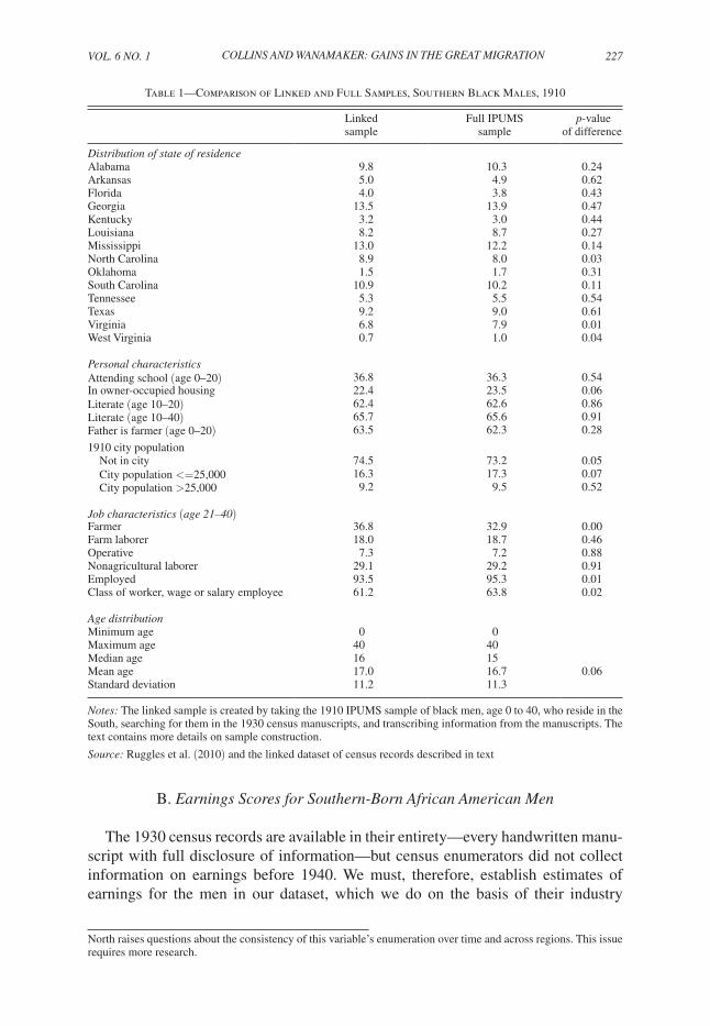
An important challenge for linked datasets is to ensure that selection into the matched sample is not biased. For example, if children from wealthier or more urban households were more likely than others to be found and matched in the 1930 manuscripts, the sample would provide a skewed perspective on the experiences of African Americans in this period. Table 1 compares the 1910 characteristics of the matched sample and the full 1910 IPUMS sample of southern black males (age 0 to 40). It is reassuring that the matched sample’s properties are very similar to those of the full sample in terms of state-of-residence, literacy and school attendance, likeli-hood of residing in owner-occupied housing, urban residence, and age distribution. The statistically significant differences (as indicated by the p-value in the last col-umn) in owner-occupied housing residence, city residence, and job characteristics are small in magnitude, suggesting limited scope for bias in the linked sample to skew our interpretation. In sum, we find no strong evidence of biased selection into the matched sample relative to the base 1910 IPUMS cross-sectional sample.
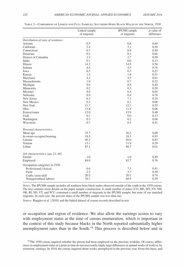
A separate check with the 1930 IPUMS cross-sectional sample of southern-born black men, age 20 to 60 (to correspond to those zero to 40 in 1910), reveals that 22.0 percent resided outside the South at the time of the 1930 census. This is close to the 20.2 percent of our matched sample who resided in the South in 1910 but not in 1930.16 For more detail, Table 2 compares the 1930 characteristics of matched black migrants in the linked sample (first column) with the 1930 IPUMS cross-sectional sample of southern-born, northern-resident black men (second column). A caveat here is that some of the northern-resident men in the IPUMS cross-section may have migrated prior to 1910, whereas all the men in the linked sample migrated after 1910. Nonetheless, we find relatively minor differences across the samples. Statistically significant differences are apparent in age (35.7 compared to 36.2), urban residence (87.1 compared to 89.7), and residence in Ohio and Missouri, but again these differences are quantitatively small.17
14 Our search criteria include a SOUNDEX version of the individual’s last name, the first three letters of the individual’s first name, the individual’s state of birth and their birth year within two years. SOUNDEX is a common algorithm used to generate alternative spellings of a surname. SOUNDEX matches include the exact last name and any reasonably close approximation to that last name. We ran a sensitivity test on our results, restricting the sample to exact last name matches and found no significant change in our estimates. See Section 1 of the online Appendix.
15 This match rate is similar to that in Long and Ferrie (2013) and Abramitzky, Boustan, and Eriksson (2012) who also create samples of linked census records.
16 We do not expect these numbers to be exactly the same because of interregional mobility prior to 1910 and sample variability.
17 A puzzling aspect of the 1930 data is the high level of literacy recorded for southern-born blacks in the North. While it is likely that some men acquired literacy between 1910 and 1930, the extremely high rate recorded in the
VOL. 6 NO. 1 227COLLINS AND WANAMAKER: GAINS IN THE GREAT MIGRATION
B. Earnings Scores for Southern-Born African American Men
The 1930 census records are available in their entirety—every handwritten manu-script with full disclosure of information—but census enumerators did not collect information on earnings before 1940. We must, therefore, establish estimates of earnings for the men in our dataset, which we do on the basis of their industry
North raises questions about the consistency of this variable’s enumeration over time and across regions. This issue requires more research.
Table 1—Comparison of Linked and Full Samples, Southern Black Males, 1910
Linked sample
Full IPUMS sample
p-value of difference
Distribution of state of residenceAlabama 9.8 10.3 0.24Arkansas 5.0 4.9 0.62Florida 4.0 3.8 0.43Georgia 13.5 13.9 0.47Kentucky 3.2 3.0 0.44Louisiana 8.2 8.7 0.27Mississippi 13.0 12.2 0.14North Carolina 8.9 8.0 0.03Oklahoma 1.5 1.7 0.31South Carolina 10.9 10.2 0.11Tennessee 5.3 5.5 0.54Texas 9.2 9.0 0.61Virginia 6.8 7.9 0.01West Virginia 0.7 1.0 0.04
Personal characteristicsAttending school (age 0–20) 36.8 36.3 0.54In owner-occupied housing 22.4 23.5 0.06Literate (age 10–20) 62.4 62.6 0.86Literate (age 10–40) 65.7 65.6 0.91Father is farmer (age 0–20) 63.5 62.3 0.28
1910 city population Not in city 74.5 73.2 0.05 City population <=25,000 16.3 17.3 0.07 City population >25,000 9.2 9.5 0.52
Job characteristics (age 21–40)Farmer 36.8 32.9 0.00Farm laborer 18.0 18.7 0.46Operative 7.3 7.2 0.88Nonagricultural laborer 29.1 29.2 0.91Employed 93.5 95.3 0.01Class of worker, wage or salary employee 61.2 63.8 0.02
Age distribution Minimum age 0 0Maximum age 40 40Median age 16 15Mean age 17.0 16.7 0.06Standard deviation 11.2 11.3
Notes: The linked sample is created by taking the 1910 IPUMS sample of black men, age 0 to 40, who reside in the South, searching for them in the 1930 census manuscripts, and transcribing information from the manuscripts. The text contains more details on sample construction.
Source: Ruggles et al. (2010) and the linked dataset of census records described in text
228 AMERICAN ECONOMIC JOURNAL: APPLIED ECONOMICS JANUARY 2014
or occupation and region of residence. We also allow the earnings scores to vary with employment status at the time of census enumeration, which is important in the context of this study because blacks in the North reported substantially higher unemployment rates than in the South.18 This process is described below and in
18 The 1930 census inquired whether the person had been employed on the previous workday. Of course, differ-ences in employment status at a point in time do not necessarily imply large differences in annual weeks of work or, by extension, earnings. In 1910, the census inquired about weeks unemployed in the previous year. From this basis, and
Table 2—Comparison of Linked and Full Samples, Southern-Born Black Males in the North, 1930
Linked sample of migrants
IPUMS sample of migrants
p-value of difference
Distribution of state of residenceArizona 0.5 0.6 0.69California 3.4 3.1 0.59Connecticut 0.7 0.9 0.50Delaware 0.2 0.3 0.66District of Columbia 3.3 3.7 0.50Idaho 0.1 0.0 0.13Illinois 14.2 14.9 0.56Indiana 4.4 4.5 0.76Iowa 0.5 0.3 0.23Kansas 1.5 1.8 0.51Maryland 4.2 4.5 0.61Massachusetts 1.0 0.7 0.22Michigan 9.6 8.9 0.45Minnesota 0.2 0.3 0.50Missouri 8.0 6.4 0.04Nebraska 0.4 0.4 0.78New Jersey 6.2 7.1 0.24New Mexico 0.3 0.1 0.08New York 11.7 12.3 0.52Ohio 13.8 11.9 0.06Pennsylvania 15.0 15.9 0.40Utah 0.1 0.0 0.13Washington 0.3 0.2 0.68Wisconsin 0.7 0.5 0.41
Personal characteristicsMean age 35.7 36.2 0.08In owner-occupied housing 18.5 18.3 0.93Literate 95.2 95.0 0.83Veteran 13.1 11.9 0.29Urban 87.1 89.7 0.01
Job characteristics (age 21– 40)Farmer 1.0 1.0 0.89Employed 84.0 83.7 0.76
Occupation categories in 1930Professional/clerical 6.6 7.3 0.41Farm 2.2 2.7 0.30Crafts/semi-skill 20.5 20.1 0.74Nonagricultural laborer 70.7 69.9 0.59
Notes: The IPUMS sample includes all southern-born black males observed outside of the south in the 1930 census. The text contains more details on the paper sample construction. A small number of states (CO, ME, MT, NV, NH, OR, RI, SD, VT, and WY) contained a small number of migrants in the IPUMS sample, but none of our matched migrants. In each case, the percent share of the IPUMS sample was less than one.
Source: Ruggles et al. (2010) and the linked dataset of census records described in text
VOL. 6 NO. 1 229COLLINS AND WANAMAKER: GAINS IN THE GREAT MIGRATION
more detail in Appendix A. We refer to workers’ “scores” throughout the analysis to emphasize that earnings per se are not reported at the individual level in the 1930 census records. The scores will allow us to estimate the returns to migration based on differences or changes in industry or occupation, region, and employment status (conditional on background characteristics). But we cannot observe differences or changes in earnings within job-region-employment status categories. Abramitzky, Boustan, and Eriksson (2012) face a similar challenge and develop an approach that is similar in spirit.
We have taken two independent routes to assigning annual earnings scores to the men in our sample. In the first method, we matched each individual to industry-specific average annual earnings data in 1928, as reported in Margo (1996) based on Lebergott (1964). Then, we adjusted the industry-level average earn-ings to reflect southern-born black-male-specific earnings levels in each industry for the South and non-South, conditional on employment status at the time of cen-sus enumeration. This adjustment factor is based on individual-level census data from the 1940 IPUMS, the first year in which enumerators collected annual earn-ings data, which pertain to the previous calendar year. For example, if construction workers earned X in 1928 according to Lebergott, and the average southern-born, southern-resident, employed, black male construction worker earned 50 percent of the average for all construction workers according to the 1940 microdata, then the assigned annual earnings score for southern, employed, black construction work-ers in the linked dataset is 0.5X.19 Note that workers who were unemployed at the time of census enumeration are assigned a different earnings score than those who were employed. If unemployed southern-born, southern-resident black males who previously worked in construction earned 25 percent of the average of all construc-tion workers in the 1940 microdata, then the assigned score would be 0.25X in the linked dataset. The industry categories in Lebergott (1964) are broad (we work with 18 industry categories), but this approach brings us as close as possible to pre-Depression, black-specific earnings levels that vary by industry, region of resi-dence, and employment status.20
using the IPUMS data, it appears that black men in the North who were unemployed at the time of enumeration worked approximately 85 percent as many weeks in the previous year as those who were employed at the time of enumeration. In 1940, the census inquired directly about weeks worked in the previous year, and the ratio was only about 65 percent.
19 There is no presumption in our approach that the unemployment rate was the same in 1930 as in 1940, only that the ratios of annual earnings for the unemployed were similar. Industry and occupation were asked of all men in the labor force in 1940. Enumerators were instructed to record the last industry and occupation for those unem-ployed. The modern definition of “labor force” did not apply in 1930, but industry and occupation were asked of all men in 1930, whether employed or unemployed. Those retired or incapable of work were to be recorded as having no occupation or industry. We report the sensitivity of our main results to alternative methods of assigning earnings to the unemployed, including an assumption that the unemployed had $0 in annual earnings, in online Appendix, Section 5. These adjustments reduce the estimated return to migration by about 10 to 16 percent compared to the paper’s base results.
20 Rather than base our estimates on Lebergott’s reported figure for agricultural workers, we dug deeper into Lebergott’s original source (US Department of Agriculture 1957) to find an income figure that covered both farmers and farm laborers, including the estimated value of perquisites and in-kind income. This figure is substantially higher than that for farm workers alone and, if overestimated, will bias our estimated returns to migration toward zero as most farm sector workers were southern residents. The adjustment factor derived from 1940 microdata is by necessity based on earnings of black farm laborers relative to other farm laborers. If within this category, black workers received more income in kind than whites, then the adjustment factor could be too low. We undertake two robustness tests to assess the sensitivity of our results to reasonable alternatives. First, we use an adjustment factor equal to the average income ratio across all nonagricultural industries rather than in agriculture itself. Second, we
230 AMERICAN ECONOMIC JOURNAL: APPLIED ECONOMICS JANUARY 2014
For an alternative and fully independent approach, we used the individual-level data from the 1960 IPUMS sample to calculate average annual earnings for southern-born black men in each three-digit occupation category within each major region (South, Northeast, Midwest, and West) by employment status.21 The within-cell average earnings are assigned directly to men in the linked dataset according to their occupation, region, and employment status. The advantages of this approach are that the 1960 microdata provide a direct measure of all black workers’ earnings, and the sample is large enough to allow detailed coverage across hundreds of occupation-region-employment-status cells for southern-born black men. Of course, 1960 is far from 1930, and this method could understate the 1930 earnings differences between migrants and nonmigrants to the extent that regional convergence in wages occurred between 1930 and 1960 among black workers.22 An offsetting factor is that the 1960 census did not count in-kind income, which may be disproportionately important for southern agricultural workers. We examine sensi-tivity to this issue in Section IV’s discussion of “base results.”
Nominal earnings score differences between migrants and nonmigrants will tend to overstate the real income gains associated with migration because price levels were, on average, higher outside the South. We rely on work by Stecker (1937), who studied cost of living (COL) differences across cities, and Koffsky (1949), who studied rural-urban cost of living differences, to adjust nominal earnings scores. Stecker’s original city-based COL measures are used for those who lived in cities, and a Koffsky-based adjustment sets relative COLs for those residing outside cities within each state. Appendix A describes this approach in more detail.
III. Evidence on Selection into the Great Migration
Different workers perceived different expected utility to living in the North rela-tive to the South, and because these expectations may have been systematically correlated with observable and unobservable characteristics (e.g., age and ability, respectively) there may have been nonrandom selection into the migrant stream. Table 3 splits the linked sample into two groups for comparison: those who left the South after 1910 and resided in the North in 1930 (“migrants”), and those who resided in the South in both 1910 and 1930 (“nonmigrants”).23 The last column of
limit the universe of individuals used to calculate the 1940 adjustment factor to only those who received less than $50 in in-kind income (the only census variable that attempts to capture in-kind pay). Our estimated magnitudes of earnings score gains for migrants are essentially unchanged. See online Appendix Section 4 for further discussion.
21 This is similar in spirit to the IPUMS “occscore” variable, which is based on median income in occupations in 1950, but it improves on the occscore variable by focusing specifically on the earnings of southern-born black men within each region, occupation, and employment status. We do not use the 1940 census here because it does not report the earnings of self-employed workers, such as farmers, and because we wanted a set of estimates that were fully independent of the first approach, which is based on a combination of Lebergott (1964) and 1940 microdata. The 1950 IPUMS sample reports income for a “sample line” subset of observations, and the resulting sample is too small to support a fine division of southern-born black workers across occupation-region-employment status cells.
22 Easterlin (1960) estimates significant interregional convergence in personal income per capita between 1930 and 1950, and Mitchener and McLean (1999) estimate convergence in income per worker between 1940 and 1960.
23 A preliminary link to the 1920 census manuscripts indicates that less than 5 percent of men in our sample are return migrants (i.e., in South in 1910, in North in 1920, and back in South in 1930). Return migrants will tend to attenuate the measured effects of migration if return migrants acquired human capital or financial capital while in the North relative to those who never left the South.
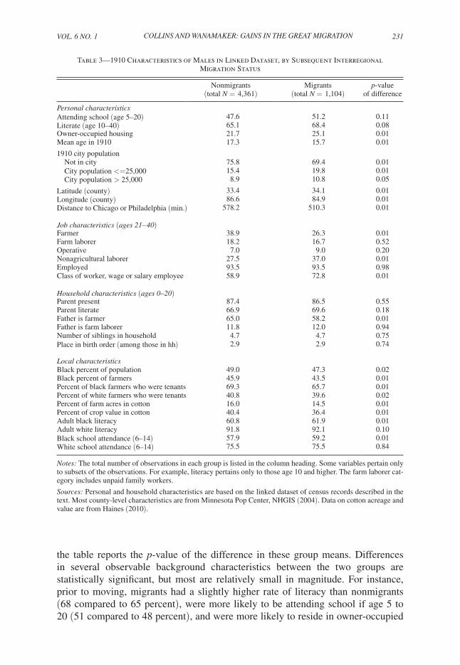
VOL. 6 NO. 1 231COLLINS AND WANAMAKER: GAINS IN THE GREAT MIGRATION
the table reports the p-value of the difference in these group means. Differences in several observable background characteristics between the two groups are statistically significant, but most are relatively small in magnitude. For instance, prior to moving, migrants had a slightly higher rate of literacy than nonmigrants (68 compared to 65 percent), were more likely to be attending school if age 5 to 20 (51 compared to 48 percent), and were more likely to reside in owner-occupied
Table 3—1910 Characteristics of Males in Linked Dataset, by Subsequent Interregional Migration Status
Nonmigrants (total N = 4,361)
Migrants (total N = 1,104)
p-value of difference
Personal characteristicsAttending school (age 5–20) 47.6 51.2 0.11Literate (age 10– 40) 65.1 68.4 0.08Owner-occupied housing 21.7 25.1 0.01Mean age in 1910 17.3 15.7 0.01
1910 city population Not in city 75.8 69.4 0.01 City population <=25,000 15.4 19.8 0.01 City population > 25,000 8.9 10.8 0.05
Latitude (county) 33.4 34.1 0.01Longitude (county) 86.6 84.9 0.01Distance to Chicago or Philadelphia (min.) 578.2 510.3 0.01
Job characteristics (ages 21– 40)Farmer 38.9 26.3 0.01Farm laborer 18.2 16.7 0.52Operative 7.0 9.0 0.20Nonagricultural laborer 27.5 37.0 0.01Employed 93.5 93.5 0.98Class of worker, wage or salary employee 58.9 72.8 0.01
Household characteristics (ages 0–20)Parent present 87.4 86.5 0.55Parent literate 66.9 69.6 0.18Father is farmer 65.0 58.2 0.01Father is farm laborer 11.8 12.0 0.94Number of siblings in household 4.7 4.7 0.75Place in birth order (among those in hh) 2.9 2.9 0.74
Local characteristicsBlack percent of population 49.0 47.3 0.02Black percent of farmers 45.9 43.5 0.01Percent of black farmers who were tenants 69.3 65.7 0.01Percent of white farmers who were tenants 40.8 39.6 0.02Percent of farm acres in cotton 16.0 14.5 0.01Percent of crop value in cotton 40.4 36.4 0.01Adult black literacy 60.8 61.9 0.01Adult white literacy 91.8 92.1 0.10Black school attendance (6–14) 57.9 59.2 0.01White school attendance (6–14) 75.5 75.5 0.84
Notes: The total number of observations in each group is listed in the column heading. Some variables pertain only to subsets of the observations. For example, literacy pertains only to those age 10 and higher. The farm laborer cat-egory includes unpaid family workers.
Sources: Personal and household characteristics are based on the linked dataset of census records described in the text. Most county-level characteristics are from Minnesota Pop Center, NHGIS (2004). Data on cotton acreage and value are from Haines (2010).
232 AMERICAN ECONOMIC JOURNAL: APPLIED ECONOMICS JANUARY 2014
housing (25 compared to 22 percent).24 On average, they were also about 70 miles closer to major destinations in the urban North, such as Chicago and Philadelphia. Differences in county-level economic characteristics are also relatively small.
Larger differences are evident in 1910 job categories for those old enough to be in the labor force. The eventual migrants had disproportionately sorted out of agricul-tural occupations prior to leaving the South; 43 percent of migrants worked as farm-ers or farm laborers in 1910 compared to 57 percent of nonmigrants. This difference extends backward at least one generation, to the cohort of parents who would have been born soon after Emancipation. In the subsample where we observe young males living with their parents in 1910 (those aged 0–20), the fathers of migrants were 7 percentage points less likely to be farmers than the fathers of nonmigrants.
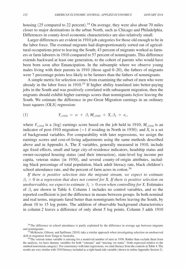
A simple metric for selection comes from examining the subset of men who were already in the labor force in 1910.25 If higher ability translated into better-paying jobs in the South and was positively correlated with subsequent migration, then the migrants should exhibit higher earnings scores than nonmigrants before leaving the South. We estimate the difference in pre-Great Migration earnings in an ordinary least squares (OLS) regression:
(1) Y i,1910 = α + β 1 M i,1930 + X i β 2 + e i ,
where Y i,1910 is a (log) earnings score based on the job held in 1910; M i,1930 is an indicator of post-1910 migration (=1 if residing in North in 1930); and X i is a set of background variables. For comparability with later regressions, we assign the earnings scores and cost-of-living adjustments using the same methods described above and in Appendix A. The X variables, generally measured in 1910, include age fixed effects, small and large city-of-residence indicators, headship status and owner-occupied housing status (and their interaction), state-level log income per capita, veteran status (in 1930), and several county-of-origin attributes, includ-ing black percentage of total population, black adult literacy rate, black children’s school attendance rate, and the percent of farm acres in cotton.26
If there is positive selection into the migrant stream, we expect to estimate β 1 > 0 in a regression that does not control for X. If there is positive selection on unobservables, we expect to estimate β 1 > 0 even when controlling for X. Estimates of β 1 are shown in Table 4. Column 1 includes no control variables, and so the reported coefficient is just the difference in means between groups. In both nominal and real terms, migrants fared better than nonmigrants before leaving the South, by about 10 to 15 log points. The addition of observable background characteristics in column 2 leaves a difference of only about 5 log points. Column 3 adds 1910
24 The difference in school attendance is partly explained by the difference in average age between migrants and nonmigrants.
25 McKenzie, Gibson, and Spillman (2010) take a similar approach when investigating selection on unobserved skill in migration from Tonga to Australia.
26 The veteran status variable is missing for a nontrivial number of men in 1930. Rather than exclude them from the analysis, we have dummy variables for both “veterans” and “missing vet status” (both expressed relative to the omitted nonveteran category). For consistency with later regressions, we omit literacy from the controls in Table 4. The results are very similar with 1910 literacy included as a right-hand side variable (shown in online Appendix Section 2).
VOL. 6 NO. 1 233COLLINS AND WANAMAKER: GAINS IN THE GREAT MIGRATION
county-of-residence fixed effects, which further reduces the estimates of β 1 to less than 2.5 log points, and the differences are no longer statistically significant.
Despite this evidence of limited selection into the migrant stream, conditional on observables, the underlying differences in earnings scores might mask differ-ences between migrants and nonmigrants in earnings within industry or occupation categories. Given the data limitations, we simply cannot see whether migrants were relatively high earners within job categories. However, for variables that are observ-able prior to migration, we find no evidence of significant differences in 1910 lit-eracy, home ownership, employment status, or residence in a large city between migrants and nonmigrants, conditional on occupation or industry category and age.27 In other words, observable characteristics that are often associated with earnings are similar for migrants and nonmigrants within job categories. It is also reassuring that the results are similar whether based on broad industry groups or narrow occupation groups. That is, using finer job categories to allow more differentiation among work-ers does not reveal larger pre-WWI differences between migrants and nonmigrants. Nonetheless, we return to this issue at the end of Section IV.
27 See online Appendix Section 7.
Table 4—1910 log Earnings Score Differences between Subsequent Migrants and Nonmigrants
(1) (2) (3)
Panel A. Earnings score based on Lebergott (1928)Nominal 0.126 0.0468 0.0221
(0.0249) (0.0198) (0.0225)Real 0.115 0.0443 0.0230
(0.0238) (0.0200) (0.0227)
Panel B. Earnings score based on IPUMS (1960)Nominal 0.152 0.0519 0.0160
(0.0287) (0.0228) (0.0264)Real 0.142 0.0495 0.0169
(0.0277) (0.0230) (0.0265)
Controls for personal, household and county characteristics in 1910
No Yes Yes
1910 County fixed effects No No Yes
Observations 2,079 2,079 2,079
Notes: Each coefficient is from a separate regression of log earnings score on migrant status (=1 if interregional migrant). Earnings are assigned according to the industry or occupation held in 1910, as described in the text. The control variables differ across the columns. Standard errors are adjusted for clustering at the household level. Column 1 has no control variables. Column 2 controls for age fixed effects, veteran status, a binary variable for blank veteran status, city status, owner-occupied housing interacted with headship status, state-level log income per capita, black percent of county population, black adult literacy rate in the county, black children’s school attendance in the county, and percent of farm acres in cotton. All variables pertain to 1910 status except veteran status. The specification in column 3 includes county fixed effects.
Sources: Linked dataset of census records. See the text and data Appendix for description of industry and occupation-based earnings scores, which draw on Lebergott (1964) and Ruggles et al. (2010).
234 AMERICAN ECONOMIC JOURNAL: APPLIED ECONOMICS JANUARY 2014
The premigration differences found in Table 4, in combination with the simple comparisons in Table 3, suggest that there was some positive selection into the migration stream, which is consistent with other views of the Great Migration (Margo 1990; Vigdor 2002). But we find that the differences are diminished substantially by including controls for background observables and county-of-origin fixed effects. This suggests that the new panel dataset may provide a useful basis for estimating the migrants’ gains, one that leaves a reasonably small scope for selection bias.
IV. Measuring the Migrants’ Gains
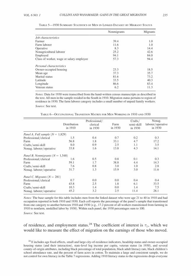
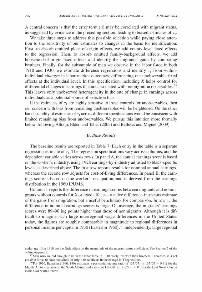
Although the migrants and nonmigrants had much in common in terms of 1910 observables (Table 3), by 1930, their lives had clearly taken divergent paths. Table 5 shows that more than half of the nonmigrants were farmers or farm laborers in 1930, compared to just 2 percent of the migrants. The migrants were disproportionately employed as operatives and unskilled laborers (in sum, nearly 60 percent). Given their overwhelmingly urban destinations, it is not surprising that migrants had higher rates of unemployment and lower rates of owner-occupancy in 1930. Table 6 shows the occupational transition matrix for migrants, nonmigrants, and the full sample of men who were age 21 to 40 in 1910 and reported an occupation in both cen-sus enumerations. For this exercise, farmers and farm workers have been grouped together, as have nonagricultural laborers and operatives, and the occupation distri-bution includes the relatively rare professional and clerical/semi-skilled categories. The majority of those who worked in farming in 1910, whether as a farmer or farm laborer, still worked in farming in 1930 (panel A, 58 percent = 33.1/56.8), espe-cially if they stayed in the South (panel B, 66 percent = 38.8/59.1). The single larg-est cell among the regional migrants in panel C is the group that shifted from farm to nonfarm labor (33.5 percent), but this group is nearly matched in size by the group that worked as nonfarm laborers before leaving the South.
The question at hand is whether these divergent career paths led to significant gains in average earnings for the migrants. It is well understood that the North was no “Promised Land.” Discrimination in labor and housing markets was pervasive (Sundstrom 1994; Meyer 2000), and events like the 1919 Chicago riot underscored the degree of racial tension in some northern cities. Moreover, recent sociological work has questioned whether the migrants gained much at all by leaving the South in later periods (Eichenlaub, Tolnay, and Alexander 2010). The linked census data provide a new and unique opportunity to measure the migrants’ gains circa 1930, while addressing the potentially confounding influence of selection.
A. Empirical Framework and Strategy
We consider the following baseline regression, estimated by OLS:
(2) Y i,1930 = λ + τ 1 M i,1930 + X i τ 2 + u i ,
where the M and X variables are similar to those described in equation (1), but Y i,1930 is log earnings score based on the observation’s 1930 industry or occupation, region
VOL. 6 NO. 1 235COLLINS AND WANAMAKER: GAINS IN THE GREAT MIGRATION
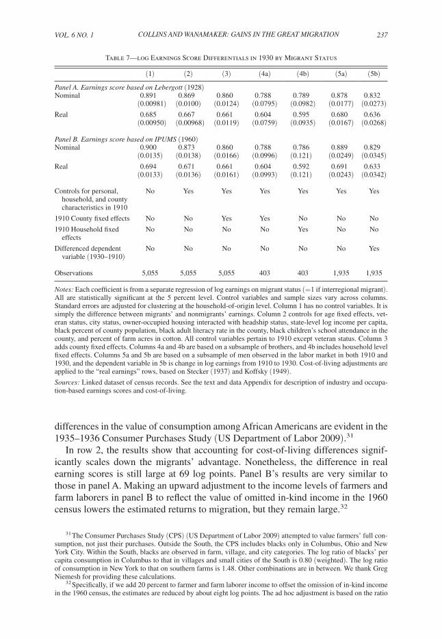
of residence, and employment status.28 The coefficient of interest is τ 1 , which we would like to measure the effect of migration on the earnings of those who moved.
28 X includes age fixed effects, small and large city-of-residence indicators, headship status and owner-occupied housing status (and their interaction), state-level log income per capita, veteran status (in 1930), and several county-of-origin attributes, including black percentage of total population, black adult literacy rate, black children’s school attendance rate, and the percent of farm acres in cotton. To maintain a large and consistent sample, we do not control for own literacy in the Table 7 regressions. Adding 1910 literacy status to the regressions drops everyone
Table 5—1930 Summary Statistics of Men in Linked Dataset by Migrant Status
Nonmigrants Migrants
Job characteristicsFarmer 39.4 1.0Farm laborer 11.6 1.0Operative 8.3 14.4Nonagricultural laborer 25.2 42.6Employed 94.1 84.0Class of worker, wage or salary employee 57.3 94.4
Personal characteristicsOwner-occupied housing 23.3 18.5Mean age 37.3 35.7Marital status 81.6 73.2Latitude 33.5 40.3Longitude 86.6 83.4Veteran status 6.2 11.3
Notes: Data for 1930 were transcribed from the hand-written census manuscripts as described in the text. All men in the sample resided in the South in 1910. Migration status pertains to region of residence in 1930. The farm laborer category includes a small number of unpaid family workers.
Source: See text.
Table 6—Occupational Transition Matrix for Men Working in 1910 and 1930
Distributionin 1910
Professional/clericalin 1930
Farmin 1930
Crafts/semi-skillin 1930
Nonag.laborer/operative
in 1930
Panel A. Full sample (N = 1,829)Professional/clerical 1.5 0.4 0.7 0.2 0.3Farm 56.8 1.8 33.1 4.7 17.2Crafts/semi-skill 8.0 0.9 2.5 1.1 3.5Nonag. laborer/operative 33.8 1.6 13.8 4.3 14.1
Panel B. Nonmigrants (N = 1,548)Professional/clerical 1.6 0.5 0.8 0.1 0.3Farm 59.1 1.7 38.8 4.4 14.3Crafts/semi-skill 7.6 0.8 3.0 1.0 2.8Nonag. laborer/operative 31.7 1.3 15.9 3.0 11.6
Panel C. Migrants (N = 281)Professional/clerical 0.7 0.0 0.0 0.4 0.4Farm 43.8 2.5 1.8 6.1 33.5Crafts/semi-skill 10.3 1.4 0.0 1.4 7.5Nonag. laborer/operative 45.2 3.2 2.5 11.4 28.1
Notes: The base sample for this table includes men from the linked dataset who were age 21 to 40 in 1910 and had occupation reported in both 1910 and 1930. Each cell reports the percentage of the panel’s sample that transitioned from one category to another between 1910 and 1930 (e.g., 17.2 percent of all workers transitioned from farming in 1910 to nonfarm, unskilled labor by 1930). Within each panel, the 1930 percentages sum to 100.
Source: See text.
236 AMERICAN ECONOMIC JOURNAL: APPLIED ECONOMICS JANUARY 2014
A central concern is that the error term (u) may be correlated with migrant status, as suggested by evidence in the preceding section, leading to biased estimates of τ 1 .
We take three steps to address this possible selection while paying close atten-tion to the sensitivity of our estimates to changes in the basis for identification. First, to absorb omitted place-of-origin effects, we add county-level fixed effects to the regression. Then, to absorb omitted family-background effects, we add household-of-origin fixed effects and identify the migrants’ gains by comparing brothers. Finally, for the subsample of men we observe in the labor force in both 1910 and 1930, we estimate difference regressions and identify τ 1 from within-individual changes in labor market outcomes, differencing out unobservable fixed effects at the individual level. In this specification, including X helps control for differential changes in earnings that are associated with premigration observables.29 This leaves only unobserved heterogeneity in the rate of change in earnings across individuals as a potential source of selection bias.
If the estimates of τ1 are highly sensitive to these controls for unobservables, then our concern with bias from remaining unobservables will be heightened. On the other hand, stability of estimates of τ 1 across different specifications would be consistent with limited remaining bias from unobservables. We pursue this intuition more formally below, following Altonji, Elder, and Taber (2005) and Bellows and Miguel (2009).
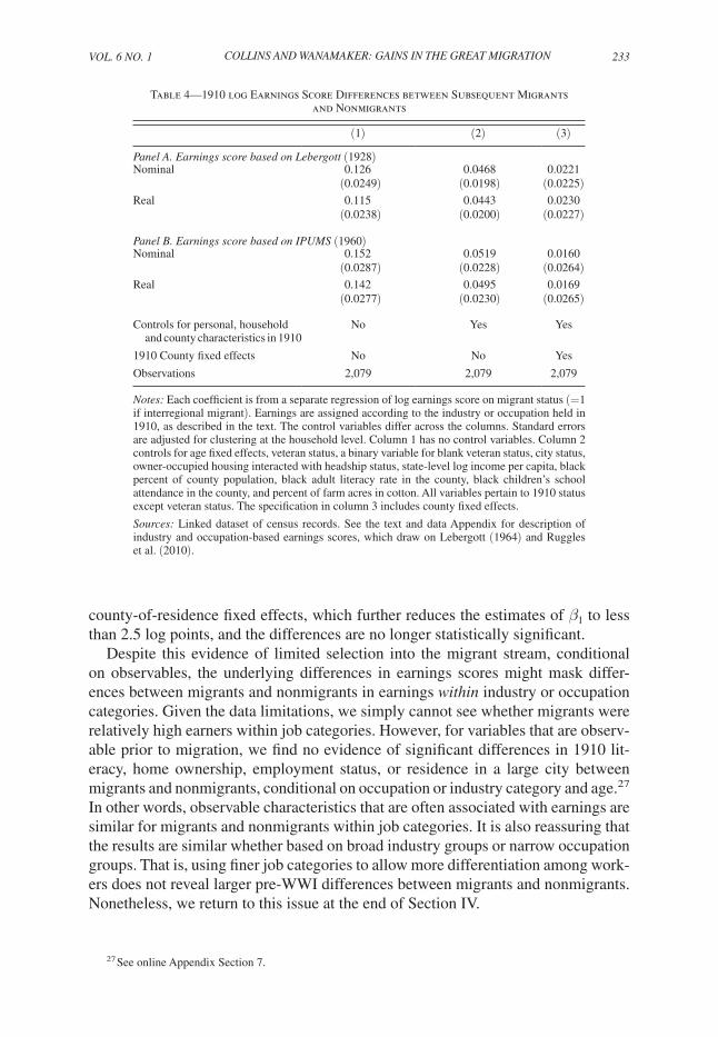
B. Base Results
The baseline results are reported in Table 7. Each entry in the table is a separate regression estimate of τ 1 . The regression specifications vary across columns, and the dependent variable varies across rows. In panel A, the annual earnings score is based on the worker’s industry, using 1928 earnings-by-industry adjusted to black-specific levels as described above. The first row reports results for nominal annual earnings, whereas the second row adjusts for cost-of-living differences. In panel B, the earn-ings score is based on the worker’s occupation, and is derived from the earnings distribution in the 1960 IPUMS.
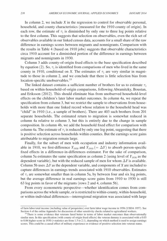
Column 1 reports the difference in earnings scores between migrants and nonmi-grants without controls for X or fixed effects—a naïve difference-in-means estimate of the gains from migration, but a useful benchmark for comparison. In row 1, the difference in nominal earnings scores is large. On average, the migrants’ earnings scores were 89–90 log points higher than those of nonmigrants. Although it is dif-ficult to imagine such large interregional wage differences in the United States today, the figures are roughly comparable in magnitude to regional differences in personal income per capita in 1930 (Easterlin 1960).30 Independently, large regional
under age 10 in 1910 but has little effect on the magnitude of the migrant-status coefficient. See Section 2 of the online Appendix.
29 Men who are old enough to be in the labor force in 1910 rarely live with their brothers. Therefore, it is not possible for us to have household-of-origin fixed effects in the change-in-Y regressions.
30 For 1930, Easterlin (1960, 140) estimates a per capita income ratio of 137/55 (ln 137/55 = 0.91) for the Middle Atlantic relative to the South Atlantic and a ratio of 115/50 (ln 115/50 = 0.83) for the East North Central to the East South Central.
VOL. 6 NO. 1 237COLLINS AND WANAMAKER: GAINS IN THE GREAT MIGRATION
differences in the value of consumption among African Americans are evident in the 1935–1936 Consumer Purchases Study (US Department of Labor 2009).31
In row 2, the results show that accounting for cost-of-living differences signif-icantly scales down the migrants’ advantage. Nonetheless, the difference in real earning scores is still large at 69 log points. Panel B’s results are very similar to those in panel A. Making an upward adjustment to the income levels of farmers and farm laborers in panel B to reflect the value of omitted in-kind income in the 1960 census lowers the estimated returns to migration, but they remain large.32
31 The Consumer Purchases Study (CPS) (US Department of Labor 2009) attempted to value farmers’ full con-sumption, not just their purchases. Outside the South, the CPS includes blacks only in Columbus, Ohio and New York City. Within the South, blacks are observed in farm, village, and city categories. The log ratio of blacks’ per capita consumption in Columbus to that in villages and small cities of the South is 0.80 (weighted). The log ratio of consumption in New York to that on southern farms is 1.48. Other combinations are in between. We thank Greg Niemesh for providing these calculations.
32 Specifically, if we add 20 percent to farmer and farm laborer income to offset the omission of in-kind income in the 1960 census, the estimates are reduced by about eight log points. The ad hoc adjustment is based on the ratio
Table 7—log Earnings Score Differentials in 1930 by Migrant Status
(1) (2) (3) (4a) (4b) (5a) (5b)
Panel A. Earnings score based on Lebergott (1928) Nominal 0.891
(0.00981)0.869
(0.0100)0.860
(0.0124)0.788
(0.0795)0.789
(0.0982)0.878
(0.0177)0.832
(0.0273)Real 0.685
(0.00950)0.667
(0.00968)0.661
(0.0119)0.604
(0.0759)0.595
(0.0935)0.680
(0.0167)0.636
(0.0268)
Panel B. Earnings score based on IPUMS (1960)Nominal 0.900
(0.0135)0.873
(0.0138)0.860
(0.0166)0.788
(0.0996)0.786
(0.121)0.889
(0.0249)0.829
(0.0345)Real 0.694
(0.0133)0.671
(0.0136)0.661
(0.0161)0.604
(0.0993)0.592
(0.121)0.691
(0.0243)0.633
(0.0342)
Controls for personal, household, and county characteristics in 1910
No Yes Yes Yes Yes Yes Yes
1910 County fixed effects No No Yes Yes No No No
1910 Household fixed effects
No No No No Yes No No
Differenced dependent variable (1930–1910)
No No No No No No Yes
Observations 5,055 5,055 5,055 403 403 1,935 1,935
Notes: Each coefficient is from a separate regression of log earnings on migrant status (=1 if interregional migrant). All are statistically significant at the 5 percent level. Control variables and sample sizes vary across columns. Standard errors are adjusted for clustering at the household-of-origin level. Column 1 has no control variables. It is simply the difference between migrants’ and nonmigrants’ earnings. Column 2 controls for age fixed effects, vet-eran status, city status, owner-occupied housing interacted with headship status, state-level log income per capita, black percent of county population, black adult literacy rate in the county, black children’s school attendance in the county, and percent of farm acres in cotton. All control variables pertain to 1910 except veteran status. Column 3 adds county fixed effects. Columns 4a and 4b are based on a subsample of brothers, and 4b includes household level fixed effects. Columns 5a and 5b are based on a subsample of men observed in the labor market in both 1910 and 1930, and the dependent variable in 5b is change in log earnings from 1910 to 1930. Cost-of-living adjustments are applied to the “real earnings” rows, based on Stecker (1937) and Koffsky (1949).Sources: Linked dataset of census records. See the text and data Appendix for description of industry and occupa-tion-based earnings scores and cost-of-living.
238 AMERICAN ECONOMIC JOURNAL: APPLIED ECONOMICS JANUARY 2014
In column 2, we include X in the regression to control for observable personal, household, and county characteristics (measured for the 1910 county of origin). In each row, the estimate of τ 1 is diminished by only one to three log points relative to the first column. This suggests that selection on observables, even the rich set of observables available in our linked census data, accounts for a small share of the raw difference in earnings scores between migrants and nonmigrants. Comparison with the results in Table 4 (based on 1910 jobs) suggests that observable characteristics circa 1910 account for a diminished portion of the difference in earnings between migrants and nonmigrants in 1930.
Column 3 adds county-of-origin fixed effects to the base specification described by equation (2). So, τ 1 is identified from comparisons of men who lived in the same county in 1910, conditional on X. The estimates of τ 1 are very similar in magni-tude to those in column 2, and we conclude that there is little selection bias from location-specific unobservables.33
The linked dataset contains a sufficient number of brothers for us to estimate τ 1 based on within-household-of-origin comparisons, following Abramitzky, Boustan, and Eriksson (2012). This should eliminate bias from unobserved household-level effects on the children’s later labor market outcomes. In column 4a, we repeat the specification from column 3, but we restrict the sample to observations from house-holds with more than one linked record whose relation to the household head was “child” in 1910 (i.e., a sample of brothers). There are 403 such brothers from 201 separate households. The estimated return to migration is somewhat reduced in column 4a relative to column 3, but this is entirely due to the change in sample composition. In column 4b, we add the household fixed effect for comparison with column 4a. The estimate of τ 1 is reduced by only one log point, suggesting that there is positive selection across households within counties. But the earnings score gains attributable to migration remain large.
Finally, for the subset of men with occupation and industry information avail-able in 1910, we first-difference Y 1930 and Y 1910 (= ΔY ) to absorb person-specific fixed effects in a difference-in-differences estimator. For the sake of comparison, column 5a estimates the same specification as column 2 (using level of Y 1930 as the dependent variable), but with the reduced sample of men for whom ΔY is available. Column 5b uses ΔY as the dependent variable, and components of X are included to capture differences in earnings trends associated with 1910 observables. Estimates of τ 1 are somewhat smaller than in column 5a, by between four and six log points, but the average difference in real earnings score gains from 1910 to 1930 is still 63 log points in favor of the migrants (rows 2 and 4, column 5b).
From every econometric perspective—whether identification comes from com-parisons across the whole sample, or is restricted to within-county, within-household, or within-individual differences—interregional migration was associated with large
of farm labor total income (including value of perquisites) over farm labor wage income in 1956 (USDA 1957). See Section 4 of the online Appendix for discussion of other sensitivity checks related to agricultural workers.
33 There is some evidence that veterans fared better in terms of labor market outcomes than observationally similar men. In this specification (with county-of-origin fixed effects) the veteran dummy is associated with a 0.03 to 0.06 higher score in 1930 (t-statistics are from 1.5 to 2.1), depending on which method is used to assign earnings scores. This could be a causal effect of military experience or evidence of positive selection into veteran status.
VOL. 6 NO. 1 239COLLINS AND WANAMAKER: GAINS IN THE GREAT MIGRATION
increases in measures of nominal and real earnings scores. We discuss the implica-tions of these gains for changes in black-white inequality in Section V.
C. Further Analysis of Unobservables and Potential Omitted Variable Bias
Because an extensive set of observable characteristics and fixed effects account for a relatively small share of the earnings difference between migrants and non-migrants in Table 7, we believe that the scope for unobservables to account for the difference is also small. Altonji, Elder, and Taber (2005) and Bellows and Miguel (2009) establish a more formal approach to assessing the plausibility that omitted variables may account for differences in outcomes. In essence, the difference in estimates of τ1 from a regression specification without controls for observables and a specification with controls provides quantitative perspective on how strong selection on unobservables would have to be, relative to selection on observables, to generate enough bias to result in an OLS estimate of τ1 equal to that observed in column 2 if the null hypothesis ( τ 1 = 0) were actually true. We provide the details of the argu-ment and calculations in Appendix B.
The key result is that selection on unobservables would have to be much stronger than selection on observables to fully account for the estimated return to migration. Given the rich set of observable background characteristics in the linked dataset, it therefore seems highly unlikely that selection on unobservables can account for a large share of the estimated returns to migration in Table 7.34
An additional concern relates to selection on unobservables and the nature of the earnings score assignments. Recall that after controlling for observables (Table 4, column 3), there is little evidence of selection into the migrant stream among workers observed in 1910 (based on earnings in their 1910 occupation or indus-try). It is possible, however, that we miss selection from within job-specific cells.35 Because score assignments are based on the earnings of black men observed in the 1940 or 1960 microdata, such selection could lead us to misinterpret the earnings advantage of migrants relative to nonmigrants. In this scenario, the estimated returns to migration would exhibit an upward bias even in a difference-in-differences frame-work akin to columns 5a and 5b of Table 7.
To develop an approach in which the assigned scores do not depend on the observed earnings of black migrants, we proceeded in two steps. First, we assigned scores to the black migrants that are equal to those of southern blacks in the same industry or occupation, conditional on employment status. In measuring the migrants’ gains, this isolates the role of industry/occupation upgrades while omitting North-South
34 Following Bellow and Miguel (2009), the results suggest that selection on unobservables would have to be between 52 and 72 times as strong as selection on observables to fully account for the estimated return to migration. Recent work by Oster (2013) points out that the Bellows and Miguel approach contains an imbedded assumption about the underlying variances of observed and unobserved covariates, and proposes an alternative application of the Altonji, Elder, and Taber (2005) result. Following Oster’s approach under extremely limiting assumptions, we still find that selection on unobservables would need to be 3–8 times as strong as selection on observables to account for the observed earnings score premium among migrants.
35 As mentioned in the previous section, we have run simple regressions of observables in 1910 on migrant sta-tus and job-specific fixed effects, to see whether there are systematic differences between nonmigrants and migrants within pre-World War I job categories. For 1910 literacy, home ownership, employment status, and large-city resi-dence, we find no statistically significant differences.
240 AMERICAN ECONOMIC JOURNAL: APPLIED ECONOMICS JANUARY 2014
differences in wage levels. Next, we adjust the migrants’ scores upward accord-ing to the regional wage premium found among whites within industry/occupation and employment status cells (based on 1940 or 1960 microdata). This incorpo-rates a regional wage premium that is insulated from unobserved selection of black migrants, though it also omits any black-specific northern wage premium within job categories (e.g., from entering a less discriminatory market). The results are comparable in magnitude to our baseline results, typically about 80 percent as large as those estimated in Table 7. These are reported in the online Appendix Section 6.
V. The Great Migration’s Contribution to African Americans’ Relative Economic Status
An important corollary of the finding that the migrants’ gains were large is that the opportunities afforded by the Great Migration may have been a central avenue for overall black economic advances in this period. To date, economists have focused primarily on two periods in which the black-white income gap narrowed rapidly—the 1940s and 1965 to 1975.36 In the 1940s, it appears that interregional migration played a positive but secondary role in blacks’ relative gains (Maloney 1994; Margo 1995), and it played only a minor role after 1964 (Donohue and Heckman 1991), by which time migration had slowed considerably. Prior to the 1940s, where our paper focuses, the story is comparatively uncharted.
We are constrained here, as elsewhere, by the lack of direct, micro-level informa-tion on workers’ earnings in this period. Consequently, our insights are limited to changes that are associated with relative improvements in job-specific and place-specific earnings scores. This may lead us to understate the change in blacks’ rela-tive status after 1910 because we cannot observe within-cell racial convergence in earnings, where a cell is defined by industry, region, and employment status, or across-cell compression of the earnings structure.37
We quantify the Great Migration’s role in raising the national average black-white earnings ratio by combining the key results from the previous section’s analy-sis of the linked dataset (i.e., the magnitude of the migrants’ gains) with information from the full IPUMS cross-sectional datasets for 1910 and 1930. Because we are interested in the national black-white earnings ratio, we need nationally representa-tive datasets for both black and white men, hence our reliance on the IPUMS cross sections. The cross-sectional data cover a broader sample of men than our linked dataset, but of course they are not as rich in terms of background characteristics.
The first step is to estimate the baseline change in the black-white earnings score ratio between 1910 and 1930, following the methods described above and in Appendix A, to assign earnings on the basis of industry, region of residence, region of birth, employment status, and race. In this framework, as emphasized above,
36 See Freeman (1973); Smith and Welch (1989); Donohue and Heckman (1991); Maloney (1994); Margo (1995); Chay (1998); and Bailey and Collins (2006).
37 This is in the spirit of Smith (1984), but our approach allows the index to reflect changes in the distribution of workers across regions and is based on pre-World War II earnings levels. Smith estimates roughly similar ratios using the 1970 income distribution, which he allows to vary across occupation and race, but not across region. His index rises from 0.455 to 0.479 from 1910 to 1930.

VOL. 6 NO. 1 241COLLINS AND WANAMAKER: GAINS IN THE GREAT MIGRATION
changes in relative earnings scores are driven chiefly by changes in industry of employment and region of residence. This abstracts from black migration’s potential general equilibrium effects, which we believe were small in comparison to the direct effects on blacks’ earnings.38 In the absence of general equilibrium effects, the full impact of the Great Migration on the black-white earnings gap would have operated through the returns to interregional migration for black migrants.
We estimate that the black-white real earnings score ratio among men ages 20 to 60 and in the labor force, increased from 0.44 to 0.47 from 1910 to 1930.39 What portion of this change is attributable to the Great Migration of African Americans? To answer this, we estimate a counterfactual black-white earnings ratio in which the gains from migration are stripped away from black men who migrated from the South between 1910 and 1930. There are two main challenges in making this calculation—one must have a tenable estimate of the gains from migration for this group of migrants, which we take from the previous section’s results, and one must have an estimate of the share of southern-born black men residing in the non-South who departed between 1910 and 1930. (Stripping the gains from migration from all migrants in 1930, including those who left the South before 1910, would over-state the role of the Great Migration per se in driving black-white convergence after 1910.)
Equation (3) describes the counterfactual estimate of black earnings in 1930:
(3) W black,1930 counterfactual = θ W non−mig,1930 + ( 1 − θ ) μ ( W mig,1930 _
e τ 1 )
+ (1 − θ)(1 − μ) W mig,1930 ,
where W is average earnings, θ is the share of nonmigrant black men (age 20–60 in 1930), μ is the share of migrants who moved between 1910 and 1930, and e τ 1 scales the post-1910 migrants’ earnings scores by the average migration effect (e.g., e 0.65 = 1.9), based on the coefficient from the previous section’s log earnings regres-sions. In this equation, “migrants” are southern-born blacks who reside outside the South in 1930; “nonmigrants” are all other blacks.
Unfortunately, it is impossible to know from the 1930 cross section when men moved from the South—the data reveal only birthplace and place of residence. We therefore estimate μ by following the geographic distribution of the southern-born black male birth cohorts that were age 0 to 40 in 1910 and 20 to 60 in 1930, based on full counts of census manuscript data. The change in the number of men from these cohorts who reside outside the South between 1910 and 1930, with an adjustment for mortality between 1910 and 1930, reflects interregional migration in
38 Our expectation is that the Great Migration tended to raise black wages in the South and lower black wages in the North. This would have offsetting effects in the numerator of the overall black-white income ratio in 1930. For empirical perspective, Boustan (2009) estimates that from 1940 and 1970, when the volume of black migration was even higher than from 1910 to 1930, migration lowered black wages in the North by 7 percent and had no effect on white wages. There is no comparable estimate for wage effects in the South.
39 This gain might seem modest relative to the changes witnessed in the 1940s, when the black-white ratio increased by about 13 percentage points (Maloney 1994, 358; Smith and Welch 1989, 522). The 1940s were a truly extraordinary decade of economic and geographic mobility as well as wage compression.
242 AMERICAN ECONOMIC JOURNAL: APPLIED ECONOMICS JANUARY 2014
that period.40 Expressed relative to the stock of such men in 1930, this provides a measure of μ.
Our best estimates of the key parameters are: θ = 0.81 and μ = 0.74. With estimates of τ 1 falling in the range of 0.6 and 0.7 in the real earnings regressions (panel A of Table 7), equation (3) implies that in the absence of the Great Migration, the counterfactual black-white real earnings score ratio would have been between 0.42 and 0.43 in 1930. This is 4 to 5 percentage points lower than the actual ratio (0.47) and slightly lower than the 1910 ratio (0.44), suggesting that blacks might have lost ground relative to whites were it not for the opportunities afforded by migration from the South. This counterfactual relative decline seems plausible given that white workers were rapidly urbanizing and acquiring high-school degrees in this period (Goldin 1998). Blacks in these birth cohorts were likely falling behind native-born whites in educational attainment (Collins and Margo 2006) and contin-ued to be shut out of most manufacturing opportunities in the South (Myrdal 1944), as well as most lines of clerical, sales, and professional work. Against these trends, regional migration appears to have been a powerful countervailing force for black economic advance in the early twentieth century. Even if the true overall black-white earnings ratio increased by more than the score-based approach suggests, the contribution associated with migration would still register as historically and quan-titatively significant.
VI. Conclusions
The pitfalls of answering questions about migration from cross-sectional datasets have been pointed out many times, but large, representative, panel datasets that span both the origins and destinations of migrants are scarce. We assembled a new dataset that links African American males between the 1910 and 1930 census manuscripts, spanning the first two decades of the Great Migration. We use the dataset to answer fundamental questions about selection into migration, the size of the migrants’ gains, and the contribution of the Great Migration to black-white income convergence.
We find some evidence of positive selection into migration. Although it is diffi-cult with existing data to pin down regional differences in the returns to education in this period, if we take the estimated returns to literacy in Collins and Margo (2006) at face value, then the pattern of black migration is not consistent with a simple interpretation of the Roy model, in which relatively low returns to education in the North would tend to lead to negatively selected migrants. A richer model, in which better-educated blacks placed a higher value on northern amenities (Margo 1990, Vigdor 2002), in which the poorest southerners were discouraged by fixed migra-tion costs (Chiquiar and Hanson 2005), or in which returns to ability (apart from
40 In 1930, we observe the stock of migrants, age 20 to 60, but not the breakdown between those who arrived before 1910 and those who arrived afterward. We can observe the stock of migrants from the same birth cohorts in 1910. Assuming this “early migrant” stock experienced mortality at the same rate as others in the cohort gives us an estimate of the surviving stock of early migrants, which we subtract from the total stock of migrants observed in 1930 to estimate the number of 1910–1930 migrants. The mortality rate is calculated using the full count of southern-born black men in the relevant birth cohorts from Ancestry.com.
VOL. 6 NO. 1 243COLLINS AND WANAMAKER: GAINS IN THE GREAT MIGRATION
education) were higher for blacks in the North would be consistent with the weakly positive selection that we observe.41
Even so, a first-order characterization of the Great Migration would emphasize how widespread it was—across rural and urban origins, across literate and illiterate men, and across premigration occupational categories. The breadth of the movement is more impressive to us than the preexisting differences between those who chose to migrate and those who chose to stay in the South. This is consistent with the sharp demand-side forces that initiated the migration, which were not specific to skilled workers, and the widespread fall in the cost of migration once networks were estab-lished. Unlike modern flows of international migrants to high-wage regions, the Great Migration was not distorted by policies that disproportionately discouraged less-skilled workers, either implicitly (e.g., by adding to the fixed costs) or explicitly (e.g., by selecting migrants based on education or occupation).
Every approach we take to measuring the migrants’ gains indicates that they were large, on average. This is true across a variety of econometric specifications, and it remains true after we adjust for cost-of-living differences. Given the empirical results, it seems implausible that omitted variables could account for a large share of the observed difference in earnings score between migrants and nonmigrants. The high volume of black migration in this period is certainly consistent with the existence of significant economic returns to migration. For comparison, the gains we estimate are similar to those estimated by Abramitzky, Boustan, and Eriksson (2012) for late nineteenth century European immigrants (around 60 log points), but are likely smaller, on average, than those earned by late twentieth century Mexican immigrants (Hanson 2006). Although it may seem surprising that such large gains could exist within a country, the facts of relative southern poverty, especially south-ern black poverty, and limited regional convergence prior to World War II are well-established. In this context, new techniques for linking census records, turning cross sections into panels, can shed light on the emergence of better integrated labor mar-kets in the United States.
Our best estimates suggest that the Great Migration was a key force in driving black-white convergence in economic status in the early twentieth century, when regional income gaps were comparatively large and when black economic mobility in the South was severely circumscribed. This is in contrast to later periods when migration made a more modest contribution to black-white convergence, especially after 1964. It is important to acknowledge that what awaited the early migrants was not a “Promised Land.” The work available to migrants was often drudgery, discrimination was common, and new evidence (Black et al. 2011) suggests that the migrants may have paid a price in terms of long-term health outcomes. Nonetheless, for the first waves of those who left the South, the gains we observe were a real and significant step away from slavery’s legacy of poverty.
41 Grogger and Hanson (2011) also show that within a Roy model framework, changing the functional form of utility from logarithmic to linear can result in positive selection from low- to high-income areas even when tradi-tionally measured returns to skill are relatively high in the home region.

244 AMERICAN ECONOMIC JOURNAL: APPLIED ECONOMICS JANUARY 2014
Appendix A: Data Appendix
A1. Occupation Codes and Industry Codes
The data for 1930 are transcribed from the hand-written manuscripts of the Census of Population, including string variables for occupation and industry and a four-digit occupation/industry code that is unique to the 1930 census. There is not a precise, one-to-one crosswalk between the 1930 occupation/industry codes and the 1950 occupation and industry codes that are fundamental to the IPUMS microdata and embedded in our data for 1910. Creating variables that correspond to the 1950-based occupation and industry classification scheme helps us make con-sistent comparisons of the 1910 and 1930 outcomes, and will facilitate use by other researchers because this classification scheme is so common. Hereafter, we use “occ1950” and “ind1950” to refer to the 1950 classification codes.
We made a number of passes through the dataset to establish and then refine the assignment of occ1950 and ind1950 codes. First, the 1930 IPUMS dataset includes both the 1950 and 1930-based classification codes, as well as the 1930 strings for occupation and industry. This gives us a starting point for assigning occ1950 and ind1950 in a manner that is consistent with the IPUMS data. By tabulating the 1930-based codes and the occupation and industry text strings, we could see whether the overwhelming majority of cases fell into a single occ1950 or ind1950 code. In many cases, there is a close correspondence, which was then applied to the assignments of occ1950 and ind1950 for the linked dataset.
For cases where the 1930-based codes and strings were less clearly concentrated in specific occ1950 or ind1950 codes in the IPUMS sample, we took two additional approaches to making assignments. A website constructed by Morse, Weintraub, and Kehs (http://stevemorse.org/census/ocodes.htm; accessed 2012), provides descriptions of the unique four-digit 1930-based coding scheme. In some cases, reading these descriptions and checking them against the descriptions for the 1950-based coding scheme (provided on the IPUMS website: http://usa.ipums.org/usa/; accessed 2012) allowed us to make occ1950 and ind1950 assignments. In other cases, simply reading the 1930 occupation and industry strings and checking them against the descriptions for the 1950-based coding scheme allowed us to make or refine the assignments.
The steps above provide the main basis for our assignments of occ1950 and ind1950, but we (and research assistants) also visually checked each observation’s combination of occupation string, industry string, occ1950 code, ind1950 code, and 1930-based code. When we found anomalies, we edited our algorithm to fix the assignment. For instance, in cases where we relied on the occupation or industry string to assign the occ1950 or ind1950 code, it is sometimes the case that the string includes a misspelling, an extra space, or a slight variation in description relative to our first pass (e.g., “grocer,” “groceries,” “grocery” or “blacksmith,” “black smith” or “Blacksmith”).
Finally, in a relatively small number of cases, we have a 1930-based code but no strings, or vice versa, or perhaps one string field is filled in but the other is not. When possible, we assigned occ1950 and/or ind1950 on a case-by-case basis with
VOL. 6 NO. 1 245COLLINS AND WANAMAKER: GAINS IN THE GREAT MIGRATION
the information at hand. For instance, a case with “farmer” listed as “occupation” but missing an industry string would typically be assigned to the ind1950 code for “agriculture.”
A2. Earnings Score Estimates
Once the occ1950 and ind1950 codes are in place, it is possible to assign annual earnings levels to each observation. The IPUMS includes a variable called “occscore” which assigns annual earnings levels to occupations based on the 1950 median earn-ings of all workers in that specific occupation category. Our approach is similar in spirit, but attempts to assign income levels that are specific to southern-born black men and vary by region. Moreover, because we also observe employment status in 1930, we can allow earnings assignments to vary on this basis.42
The first set of annual earnings assignments are based on fairly broad industry-level data from 1928. These data are reported in Historical Statistics of the United States (Margo 1996, 2–273) and were originally compiled by Lebergott (1964, 525–527). These industries are mapped as closely as possible to the corresponding industries based on the ind1950 codes, yielding 18 industry categories.43 Because there is considerable scope for differences between the earnings of black men and the “full time equivalent earnings” of all workers (from Lebergott 1964), we have made black-specific adjustments to the Lebergott data as follows. Using the 1940 IPUMS microdata, we calculated the mean earnings of southern-born black men, age 18–65, in each industry/region/employment-status cell ( Y ire ). The sample includes wage and salary workers who earned more than $0 in the previous year and were in the labor force at the time of the census. In this case, “region” pertains to South or non-South residence (reflecting migration), and “employment status” pertains to employed or unemployed. For each cell, we divide this black-specific earnings figure ( Y ire ) by the average for all wage and salary workers with positive earnings, age 18–65, who worked for the full year (48 weeks or more) in industry i( Y i ). Then, for each observation in the linked dataset, the ratio ( Y ire / Y i ) is multiplied by the annual earnings by industry from Lebergott to estimate the annual earnings of southern-born black men by industry, region of residence, and employment status.44
42 This flexibility (by employment status) may be useful to the extent that unemployment is more or less preva-lent in 1930 than in 1940 or 1960, the years that supply microdata on the previous year’s earnings by job, location, and employment status category.
43 In some instances, the coverage from Lebergott is not complete, and we make minor adjustments to fill in gaps. For example, Lebergott does not have earnings for those in the “business and repair services” category, but the 1940 IPUMS data suggest that those in business and repair services had nearly the same average earnings as those in professional services (which is available from Lebergott). Industry-level earnings can be assigned accordingly. Likewise, Lebergott does not have a separate “entertainment and recreation” category, but the IPUMS data show that entertainment and recreation workers earned about 1.17 times more than those in the wholesale or retail trade category (which is available from Lebergott). Again, earnings can be assigned accordingly.
44 Not surprisingly, the ratio ( Y ire / Y i ) is almost always less than one—black men earn less than the national average in each industry. An exception is male migrants employed in household service because the denominator includes a large number of southern black female domestic servants. In cells where there are few (less than ten) available observations in the 1940 IPUMS sample, we assign ratios from a collection of broader but similar industry categories. This is most commonly an issue for “unemployed” cells since a small share of black men were unem-ployed. For example, the most common substitution is made for unemployed men who last worked in specific non-personal-service industries (e.g., entertainment, medical, legal services, education), where we use an earnings ratio
246 AMERICAN ECONOMIC JOURNAL: APPLIED ECONOMICS JANUARY 2014
We make one substantial adjustment to the base Lebergott (1964) data. Following Lebergott’s description of sources and replicating his earnings estimate for agricul-ture, it is clear that his figure pertains to hired labor. Using the same sources (USDA 1957), we calculated an average earnings figure that also includes the net income of farmers in 1928. This raises the base assignment of income for those in agriculture, including a significant share of nonmigrants.
To construct a second and independent set of earnings estimates, we started with the comparatively large 1960 IPUMS dataset. The 1960 dataset has the advantage of reporting both wage and self-employment income in the previous year for a large number of southern-born black men. This allows us to use three-digit occupation codes and observe self-employed farmers. After sorting the men (age 18 to 65, in the labor force, worked at least one week in the previous year) into detailed cells defined by four region of residence categories (Northeast, Midwest, South, and West) and three-digit occupation codes, we collapsed the data and retained the mean value of earnings within each cell. In cases where there were less than ten observations in the cell, we moved to broader region-of-residence groupings (South and non-South) to estimate mean earnings. If there were still less than ten observations, we moved to broader occupational groupings (basically one-digit of detail), while returning to the original four region-of-residence distinctions.
Again, this provides a basis for the earnings score assignment that is com-pletely independent from the industry-based assignments described above. The disadvantage is that between 1930 and 1960, the South began convergence on the non-South in terms of income (Mitchener and McLean 1999), and the overall wage distribution compressed in the 1940s (Goldin and Margo 1992). So, this approach may tend to underestimate the earnings differences between migrants and nonmigrants circa 1930.
A3. Cost of Living Adjustments
Williamson and Lindert (1980) provide one basis for adjusting nominal earn-ings for geographic differences in the cost of living circa 1930. Their data are reported at the state level and are built up from city-level information located in Stecker (1937). Williamson and Lindert essentially create a weighted average of cost-of-living at the state level by adjusting Stecker’s city-based figures according to the share of the labor force in agriculture in each state and an estimate of the difference in price levels between rural and urban areas. This adjustment incor-porates Koffsky’s (1949) estimate of the difference between farm and city price levels in 1941. Higher shares working in nonagricultural jobs imply more weight on the city-based price levels.
The approach we favor works with the same underlying price index data, but it stays closer to Stecker’s city-specific data when possible. This allows the COL measure to correspond more closely to the black population distribution (predominantly urban), whereas the original Williamson and Lindert estimates pertain to the whole
from pooling observations from such industries together (e.g., pooling workers from communications/utilities, entertainment/recreation, medical/hospital, legal, education, religious/nonprofit, and government industries).

VOL. 6 NO. 1 247COLLINS AND WANAMAKER: GAINS IN THE GREAT MIGRATION
population of each state. First, we assign Stecker’s city-specific values to those liv-ing in the cities she covered (e.g., this fixes Chicago relative to Birmingham). Then, for residents of cities not covered by Stecker but with at least 25,000 residents, we assign values that are equal to the black population-weighted average for Stecker-covered cities in the same state (e.g., this assigns Montgomery the average cost-of-living of Birmingham and Mobile). Then, we assign values to those in places with less than 25,000 residents by applying the same “Koffsky adjustment” factor as Williamson and Lindert—this scales down Stecker’s city-based values for that state by a factor of 1.205. In a few states, Stecker covers no cities, the most important of which for our purposes is Mississippi, where we use Alabama’s data as a substitute.
We attach one significant caveat to these estimates. Stecker’s figures are not spe-cific to African Americans, and it is possible that black city dwellers faced a higher cost of living than white city dwellers, arguably due to discrimination and residential segregation. In this case, the cost-of-living adjustments may be too small and real wages may appear too large. On the other hand, many blacks in northern cities had access to goods, services, and amenities that were unavailable in the rural South (e.g., running water, urban entertainment, political rights), which is not captured in the COL differences. The online Appendix presents results calculated using the COL adjustments based on Williamson and Lindert (1980).
Appendix B: Assessing the Plausibility that Omitted Variable Bias Accounts for the Estimated Gains from Migration
We follow Bellows and Miguel (2009), who build on the work of Altonji, Elder, and Taber (2005), to assess the impact of omitted variable bias in a linear OLS framework. Converting the Bellows and Miguel structure to our context, suppose earnings of African Americans in 1930 are determined by the following equation:
(B1) Y i = τ 1 M i,1930 + τ 2 Z i + ε i ,
where Y i represents earnings, M i,1930 = 1 if the individual resides in the north in 1930 and Z i is a vector of individual characteristics. The coefficient of interest, τ 1 , is measured and reported in Table 7. However, when components of Z i are unobserved, τ 1 suffers from standard omitted variables bias and
plim τ ̂ 1OLS,NC = τ 1 + τ 2 Cov( M 1930 , Z)
__ Var( M 1930 )
,
where τ ̂ 1OLS,NC is the OLS estimate of τ 1 with no controls. Suppose, then, that Z i consists of observable components X i and an unobservable component q i such that
Z i = X i + q i .
Then, the earnings equation can be written as
(B2) Y i = τ 1 M i,1930 + τ 2 X i + τ 2 q i + ε i ,
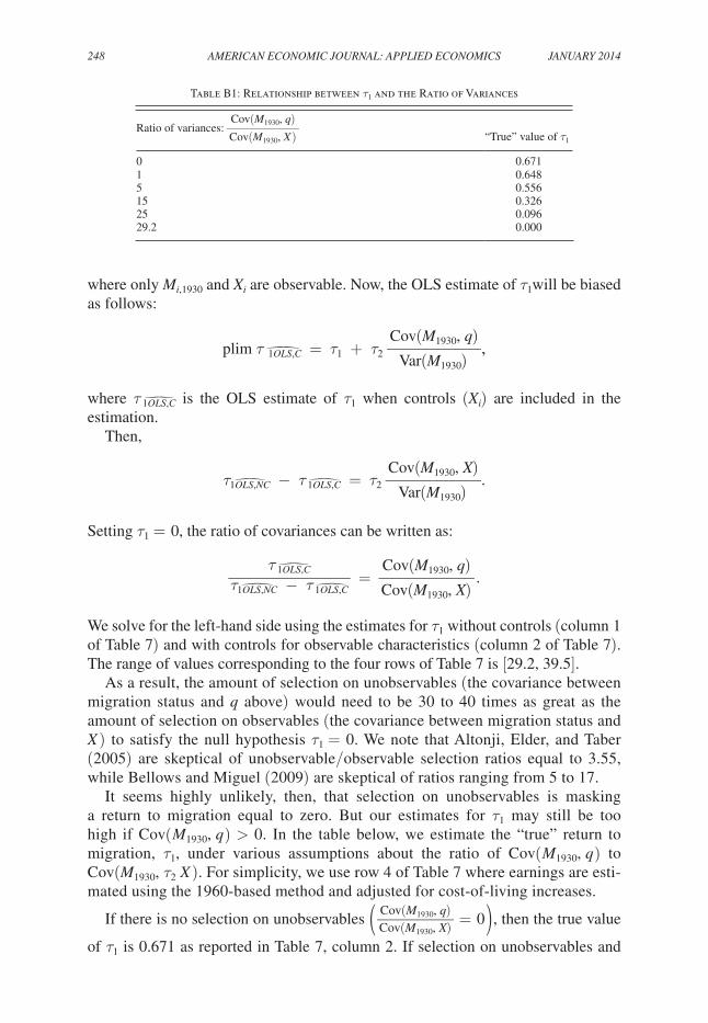
248 AMERICAN ECONOMIC JOURNAL: APPLIED ECONOMICS JANUARY 2014
where only M i,1930 and X i are observable. Now, the OLS estimate of τ 1 will be biased as follows:
plim τ ̂ 1OLS,C = τ 1 + τ 2 Cov( M 1930 , q)
_ Var( M 1930 )
,
where τ ̂ 1OLS,C is the OLS estimate of τ 1 when controls ( X i ) are included in the estimation.
Then,
τ ̂ 1OLS,NC − τ ̂ 1OLS,C = τ 2 Cov( M 1930 , X)
__ Var( M 1930 )
.
Setting τ 1 = 0, the ratio of covariances can be written as:
τ ̂ 1OLS,C __ τ ̂ 1OLS,NC − τ ̂ 1OLS,C
= Cov( M 1930 , q)
__ Cov( M 1930 , X)
.
We solve for the left-hand side using the estimates for τ 1 without controls ( column 1 of Table 7) and with controls for observable characteristics (column 2 of Table 7). The range of values corresponding to the four rows of Table 7 is [29.2, 39.5].
As a result, the amount of selection on unobservables (the covariance between migration status and q above) would need to be 30 to 40 times as great as the amount of selection on observables (the covariance between migration status and X ) to satisfy the null hypothesis τ 1 = 0. We note that Altonji, Elder, and Taber (2005) are skeptical of unobservable/observable selection ratios equal to 3.55, while Bellows and Miguel (2009) are skeptical of ratios ranging from 5 to 17.
It seems highly unlikely, then, that selection on unobservables is masking a return to migration equal to zero. But our estimates for τ 1 may still be too high if Cov ( M 1930 , q ) > 0. In the table below, we estimate the “true” return to migration, τ 1 , under various assumptions about the ratio of Cov ( M 1930 , q ) to Cov( M 1930 , τ 2 X ). For simplicity, we use row 4 of Table 7 where earnings are esti-mated using the 1960-based method and adjusted for cost-of-living increases.
If there is no selection on unobservables ( Cov( M 1930 , q) _
Cov( M 1930 , X) = 0 ) , then the true value
of τ 1 is 0.671 as reported in Table 7, column 2. If selection on unobservables and
Table B1: Relationship between τ 1 and the Ratio of Variances
Ratio of variances: Cov( M 1930 , q)
__ Cov( M 1930 , X )
“True” value of τ 1
0 0.6711 0.6485 0.55615 0.32625 0.09629.2 0.000

VOL. 6 NO. 1 249COLLINS AND WANAMAKER: GAINS IN THE GREAT MIGRATION
observables are equivalent, i.e., Cov( M 1930 , q) _
Cov( M 1930 , X) = 1, τ 1 is reduced by 2.3 log points to
0.648. Only if the ratio of selection on unobservables to selection on observables rises above 7 does the model predict a return to migration below 50 log points. Again, we conclude that the returns to interregional migration were large and our estimates are unlikely to be biased by selection on unobserved characteristics.
REFERENCES
Abramitzky, Ran, Leah Platt Boustan, and Katherine Eriksson. 2012. “Europe’s Tired, Poor, Huddled Masses: Self-Selection and Economic Outcomes in the Age of Mass Migration.” American Eco-nomic Review 102 (5): 1832–56.
Altonji, Joseph G., Todd E. Elder, and Christopher R. Taber. 2005. “Selection on Observed and Unob-served Variables: Assessing the Effectiveness of Catholic Schools.” Journal of Political Economy 113 (1): 151–84.
Bailey, Martha J., and William J. Collins. 2006. “The Wage Gains of African-American Women in the 1940s.” Journal of Economic History 66 (3): 737–77.
Bellows, John, and Edward Miguel. 2009. “War and Local Collective Action in Sierra Leone.” Journal of Public Economics 93 (11–12): 1144–57.
Black, Dan A., Seth G. Sanders, Evan J. Taylor, and Lowell J. Taylor. 2011. “The Impact of the Great Migration on Mortality of African Americans: Evidence from the Deep South.” http://www.frbat-lanta.org/documents/news/conferences/11employment_education_black.pdf.
Blanchflower, David G., Jumana Saleheen, and Chris Shadforth. 2007. “The Impact of the Recent Migration from Eastern Europe on the UK Economy.” Institute for the Study of Labor (IZA) Dis-cussion Paper 2615.
Bodnar, John, Roger Simon, and Michael P. Weber. 1982. Lives of Their Own: Blacks, Italians, and Poles in Pittsburgh, 1900–1960. Urbana-Champaign, IL: University of Illinois Press.
Borjas, George. 1987. “Self-Selection and the Earnings of Immigrants.” American Economic Review 77 (4): 531–53.
Boustan, Leah Platt. 2009. “Competition in the Promised Land: Black Migration and Racial Wage Convergence in the North, 1940–1970.” Journal of Economic History 69 (3): 755–82.
Carrington, William J., Enrica Detragiache, and Tara Vishwanath. 1996. “Migration with Endoge-nous Moving Costs.” American Economic Review 86 (4): 909–30.
Chay, Kenneth Y. 1998. “The Impact of Federal Civil Rights Policy on Black Economic Progress: Evidence from the Equal Employment Opportunity Act of 1972.” Industrial and Labor Relations Review 51 (4): 608–32.
Chay, Kenneth, and Kaivan Munshi. 2012. “Black Networks after Emancipation: Evidence from Reconstruction and the Great Migration.” http://www.stanford.edu/group/SITE/archive/SITE_2012/2012_segment_1/2012_SITE_Segment_1_papers/munshi.pdf.
Chiquiar, Daniel, and Gordon H. Hanson. 2005. “International Migration, Self-Selection, and the Dis-tribution of Wages: Evidence from Mexico and the United States.” Journal of Political Economy 113 (2): 239–81.
Clemens, Michael A. 2011. “Economics and Emigration: Trillion-Dollar Bills on the Sidewalk?” Jour-nal of Economic Perspectives 25 (3): 83–106.
Collins, William J. 1997. “When the Tide Turned: Immigration and the Delay of the Great Black Migration.” Journal of Economic History 57 (3): 607–32.
Collins, William J. 2000. “African-American Economic Mobility in the 1940s: A Portrait from the Palmer Survey.” Journal of Economic History 60 (3): 756–81.
Collins, William J., and Marianne H. Wanamaker. 2014. “Selection and Economic Gains in the Great Migration of African Americans: New Evidence from Linked Census Data: Dataset.” American Economic Journal: Applied Economics. http://dx.doi.org/10.1257/app.6.1.220.
Collins, William J., and Robert A. Margo. 2006. “Historical Perspectives on Racial Differences in Schooling in the United States.” In Handbook of the Economics of Education, Vol. 1, edited by Eric Hanushek and Finis Welch, 107–54. Amsterdam: North-Holland.
Doetsch, Ethan. 2011. “Selection and Success during the Great Migration: New Evidence on the Roles of Race, Urban Origins, and Skills from 1890–1930.” Unpublished.

250 AMERICAN ECONOMIC JOURNAL: APPLIED ECONOMICS JANUARY 2014
Donohue, John J., III, and James Heckman. 1991. “Continuous Versus Episodic Change: The Impact of Civil Rights Policy on the Economic Status of Blacks.” Journal of Economic Literature 29 (4): 1603–43.
Easterlin, Richard. 1960. “Interregional Differences in Per Capita Income, Population, and Total Income, 1840-1950.” In Trends in the American Economy in the Nineteenth Century, 73–140. Princeton: Princeton University Press.
Eichenlaub, Suzanne C., Stewart E. Tolnay, and J. Trent Alexander. 2010. “Moving Out but Not Up: Economic Outcomes in the Great Migration.” American Sociological Review 75 (1): 101–25.
Eldridge, Hope T., and Dorothy Swaine Thomas. 1964. Population Redistribution and Economic Growth, United States, 1870–1950. Vol. 3, Demographic Analyses and Interrelations. Philadelphia: American Philosophical Society.
Foote, Christopher L., Warren C. Whatley, and Gavin Wright. 2003. “Arbitraging a Discriminatory Labor Market: Black Workers at the Ford Motor Company, 1918–1947.” Journal of Labor Econom-ics 21 (3): 493–532.
Freeman, Richard B. 1973. “Changes in the Labor Market for Black Americans, 1948–72.” Brookings Papers on Economic Activity 4 (1): 67–132.
Gill, Flora. 1979. Economics and the Black Exodus: An Analysis of Negro Emigration from the South-ern United States, 1910-70. New York: Garland Publishing.
Goldin, Claudia. 1998. “America’s Graduation from High School: The Evolution and Spread of Sec-ondary Schooling in the Twentieth Century.” Journal of Economic History 58 (2): 345–74.
Goldin, Claudia, and Robert A. Margo. 1992. “The Great Compression: The Wage Structure in the United States at Mid-Century.” Quarterly Journal of Economics 107 (1): 1–34.
Gottlieb, Peter. 1987. Making Their Own Way: Southern Blacks’ Migration to Pittsburgh, 1916–1930. Chicago: University of Illinois Press.
Grogger, Jeffrey, and Gordon H. Hanson. 2011. “Income Maximization and the Selection and Sorting of International Migrants.” Journal of Development Economics 95 (1): 42–57.
Haines, Michael R., and Inter-university Consortium for Political and Social Research. 2010. His-torical, Demographic, Economic, and Social Data: The United States, 1790-2002 [computer file]. ICPSR02896-v3. Ann Arbor, MI: ICPSR [distributor]. doi:10.3886/ICPSR02896.v3.
Hanson, Gordon H. 2006. “Illegal Migration from Mexico to the United States.” Journal of Economic Literature 44 (4): 869–924.
Hatton, Timothy J., and Jeffrey G. Williamson. 1998. The Age of Mass Migration: Causes and Eco-nomic Impact. New York: Oxford University Press.
Hatton, Timothy J., and Jeffrey G. Williamson. 2003. “Demographic and Economic Pressure on Emi-gration out of Africa.” Scandinavian Journal of Economics 105 (3): 465–86.
Higgs, Robert. 1976. “The Boll Weevil, the Cotton Economy, and Black Migration 1910–1930.” Agri-cultural History 50 (2): 335–50.
Higgs, Robert. 1982. “Accumulation of Property by Southern Blacks before World War I.” American Economic Review 72 (4): 725–37.
Koffsky, Nathan. 1949. “Part II: Farm and Urban Purchasing Power.” In Studies in Income and Wealth, Vol. 11, 151–220. New York: National Bureau of Economic Research.
Kousser, J. Morgan. 1974. The Shaping of Southern Politics: Suffrage Restriction and the Establish-ment of the One-Party South, 1880–1910. New Haven: Yale University Press.
Lebergott, Stanley. 1964. Manpower in Economic Growth: The American Record since 1800. New York: McGraw-Hill.
Lemann, Nicholas. 1991. The Promised Land: The Great Black Migration and How It Changed Amer-ica. New York: Alfred A. Knopf, Inc.
Lewis, Edward Erwin. 1931. The Mobility of the Negro: A Study in the American Labor Supply. New York: Columbia University Press.
Lieberson, Stanley. 1978. “A Reconsideration of the Income Differences Found between Migrants and Northern-born Blacks.” American Journal of Sociology 83 (4): 940–66.
Logan, Trevon D. 2009. “Health, Human Capital, and African-American Migration before 1910.” Explorations in Economic History 46 (2): 169–85.
Long, Jason, and Joseph Ferrie. 2013. “Intergenerational Occupational Mobility in Great Britain and the United States since 1850.” American Economic Review 103 (4): 1109–37.
Long, Larry H., and Lynne R. Heltman. 1975. “Migration and Income Differences between Black and White Men in the North.” American Journal of Sociology 80 (6): 1391–1409.
Maloney, Thomas N. 1994. “Wage Compression and Wage Inequality between Black and White Males in the United States, 1940–1960.” Journal of Economic History 54 (2): 358–81.
VOL. 6 NO. 1 251COLLINS AND WANAMAKER: GAINS IN THE GREAT MIGRATION
Maloney, Thomas N. 2001. “Migration and Economic Opportunity in the 1910s: New Evidence on African-American Occupational Mobility in the North.” Explorations in Economic History 38 (1): 147–65.
Margo, Robert A. 1988. “Schooling and the Great Migration.” National Bureau of Economic Research (NBER) Working Paper 2697.
Margo, Robert A. 1990. Race and Schooling in the South 1880-1950: An Economic History. Chicago: University of Chicago Press.
Margo, Robert A. 1995. “Explaining Black-White Wage Convergence, 1940–1950.” Industrial and Labor Relations Review 48 (3): 470–81.
Margo, Robert A. 1996. “Wages.” In Historical Statistics of the United States, Millennial Edition, edited by Susan B. Carter et al. New York: Cambridge University Press.
McKenzie, David, John Gibson, and Steven Stillman. 2010. “How Important is Selection? Experimen-tal vs. Non-Experimental Measures of the Income Gains from Migration.” Journal of the European Economic Association 8 (4): 913–45.
Meyer, Stephen Grant. 2000. As Long As They Don’t Move Next Door: Segregation and Racial Conflict in American Neighborhoods. Lanham: Rowman & Littlefield.
Minnesota Population Center. 2011. National Historical Geographic Information System: Version 2.0. Minneapolis, MN: University of Minnesota.
Mitchener, Kris James, and Ian W. McLean. 1999. “U.S. Regional Growth and Convergence, 1880–1980.” Journal of Economic History 59 (4): 1016–42.
Moretti, Enrico. 2011. “Local Labor Markets.” In Handbook of Labor Economics, Vol. 4B, edited by Orley Ashenfelter and David Card, 1237–1313. San Diego: North-Holland.
Morse, Stephen P., Joel D. Weintraub, and David R. Kehs. 2002. “Deciphering Occupation Codes Appended to the 1930 Census in One Step.” http://stevemorse.org/census/ocodes.htm (accessed March 1, 2011 through October 18, 2012).
Myrdal, Gunnar. 1944. An American Dilemma: The Negro Problem and Modern Democracy. New York: Harper & Brothers Publishers.
Naidu, Suresh. 2010. “Recruitment Restrictions and Labor Markets: Evidence from the Postbellum U.S. South.” Journal of Labor Economics 28 (2): 413–45.
Oster, Emily. 2013. “Unobservable Selection and Coefficient Stability: Theory and Validation.” Uni-versity of Chicago Working Paper.
Ransom, Roger L., and Richard Sutch. 2001. One Kind of Freedom: The Economic Consequences of Emancipation, Second Edition. New York: Cambridge University Press, (Orig. pub. 1977).
Roback, Jennifer. 1982. “Wages, Rents, and the Quality of Life.” Journal of Political Economy 90 (6): 1257–78.
Rosenbloom, Joshua L. 2002. Looking for Work, Searching for Workers: American Labor Markets dur-ing Industrialization. New York: Cambridge University Press.
Roy, A. D. 1951. “Some Thoughts on the Distribution of Earnings.” Oxford Economic Papers 3 (2): 135–46.
Ruggles, Steven, J. Trent Alexander, Katie Genadek, Ronald Goeken, Matthew B. Schroeder, and Mat-thew Sobek. 2010. Integrated Public Use Microdata Series: Version 5.0 [Machine-readable data-base]. Minneapolis: University of Minnesota.
Sjaastad, Larry A. 1962. “The Costs and Returns of Human Migration.” Journal of Political Economy 70 (5): 80–93.
Smith, James P. 1984. “Race and Human Capital.” American Economic Review 74 (4): 685–98.Smith, James P., and Finis R. Welch. 1989. “Black Economic Progress After Myrdal.” Journal of Eco-
nomic Literature 27 (2): 519–64.Stecker, Margaret Loomis. 1937. Intercity Differences in Costs of Living in March 1935, 59 Cities.
Works Progress Administration, Division of Social Research, Research Monograph XII. Washing-ton, DC, March.
Sundstrom, William A. 1994. “The Color Line: Racial Norms and Discrimination in Urban Labor Mar-kets, 1910–1950.” Journal of Economic History 54 (2): 382–96.
Todaro, Michael P. 1969. “A Model of Labor Migration and Urban Unemployment in Less Developed Countries.” American Economic Review 59 (1): 138–48.
Tolnay, Stewart E. 2003. “The African American ‘Great Migration’ and Beyond.” Annual Review of Sociology 29: 209–32.
Tolnay, Stewart E. and E. M. Beck. 1995. A Festival of Violence: An Analysis of Southern Lynchings, 1882–1930. Champaign: University of Illinois Press.
U.S. Department of Agriculture. 1957. Major Statistical Series of the U.S. Department of Agriculture. Volumes 3 and 7. Washington, DC: Government Printing Office.
252 AMERICAN ECONOMIC JOURNAL: APPLIED ECONOMICS JANUARY 2014
U.S. Department of Labor. 1919. Negro Migration in 1916–17. Washington, DC: Government Print-ing Office.
U.S. Department of Labor. 2009. “Study of Consumer Purchases in the United States, 1935–1936.” ICPSR 08908-v3. Ann Arbor, MI: Inter-university Consortium for Political and Social Research [distributor], 2009-06-29. doi:10.3886/ICPSR08908.v3.
Vickery, William Edward. 1977. The Economics of the Negro Migration, 1900–1960. New York: Arno Press.
Vigdor, Jacob L. 2002. “The Pursuit of Opportunity: Explaining Selective Black Migration.” Journal of Urban Economics 51 (3): 391–417.
Whatley, Warren C. 1990. “Getting a Foot in the Door: ‘Learning,’ State Dependence, and the Racial Integration of Firms.” Journal of Economic History 50 (1): 43–66.
Wilkerson, Isabel. 2010. The Warmth of Other Suns: The Epic Story of America’s Great Migration. New York: Random House.
Williams, Heather Andrea. 2005. Self-Taught: African American Education in Slavery and Freedom. Chapel Hill: University of North Carolina Press.
Williamson, Jeffrey G., and Peter H. Lindert. 1980. American Inequality: A Macroeconomic History. New York: Academic Press.
Woodson, Carter G. 2002. A Century of Negro Migration. Mineola, NY: Dover Publications, (Orig. pub. 1918).
Woodward, C. Vann. 1974. The Strange Career of Jim Crow, Third Revised Edition. New York: Oxford University Press.
Wright, Gavin. 1986. Old South, New South: Revolutions in the Southern Economy since the Civil War. New York: Basic Books.
Wright, Gavin. 1987. “Postbellum Southern Labor Markets.” In Quantity and Quiddity: Essays in U.S. Economic History, edited by Peter Kilby, 98–134. Middletown, CT: Wesleyan University Press.
Zhao, Yaohui. 1999. “Leaving the Countryside: Rural-to-Urban Migration Decisions in China.” Ameri-can Economic Review 89 (2): 281–86.

This article has been cited by:
1. Catherine G. Massey. 2017. Playing with matches: An assessment of accuracy in linkedhistorical data. Historical Methods: A Journal of Quantitative and Interdisciplinary History 63, 1-15.[CrossRef]
2. Ramon Ramon-Muñoz, Josep-Maria Ramon-Muñoz. 2016. Sibship size and the biologicalstandard of living in industrial Catalonia, c.1860–c.1920: a case study. The History of the Family1-31. [CrossRef]
3. Dan A. Black, Seth G. Sanders, Evan J. Taylor, Lowell J. Taylor. 2015. The Impact of the GreatMigration on Mortality of African Americans: Evidence from the Deep South. American EconomicReview 105:2, 477-503. [Abstract] [View PDF article] [PDF with links]