security constrained optimal power ﬂow problems

Bachelor Thesis

January 14, 2018

Security constrained optimal power flow problemsA study of different optimization techniques

Samuel A. Cruz Alegría

Abstract

The electrical power grid is a critical infrastructure, and in addition to economic dispatch, the grid operation shouldbe resilient to failures of its components. Increased penetration of renewable energy sources is placing greater stresson the grid, shifting operation of the power grid equipment towards their operational limits. Thus, any unexpectedcontingency could be critical to the overall operation. Consequently, it is essential to operate the grid with a focus onthe security measures. Security constrained optimal power flow imposes additional security constraints to the optimalpower flow problem. It aims for minimum adjustments in the base precontingency operating state, such that in theevent of any contingency, the postcontingency states will remain secure and within operating limits. For a realisticpower network, however, with numerous contingencies considered, the overall problem size becomes intractable forsingle-core optimization tools in short time frames for real-time industrial operations, such as rapid resolution of newoptimal operating conditions over changing network demands, or real-time electricity market responses to electricityprices. Optimization software becomes a major bottleneck for the energy system modellers. Given that optimizationsoftware becomes a major bottleneck, this thesis aims to explore different optimization frameworks; specifically, itwill cover the IPOPT and Optizelle optimization frameworks.

AdvisorProf. Olaf SchenkAssistantsJuraj Kardoš, Dr. Drosos Kourounis

Advisor’s approval (Prof. Olaf Schenk): Date:

Acknowledgements

I would like to thank my advisors Prof. Dr. Olaf Schenk, Juraj Kardoš, and Dr. Drosos Kourounis, this work couldnot have been accomplished without all of their help and support. In particular, I would like to thank Juraj Kardošfor his constant support and guidance.

Contents

1 Introduction 21.1 Project description . . . . . . . . . . . . . . . . . . . . . . . . . . . . . . . . . . . . . . . . . . . . . . . . . . . . 21.2 Linearity and nonlinearity . . . . . . . . . . . . . . . . . . . . . . . . . . . . . . . . . . . . . . . . . . . . . . . . 31.3 Convex functions . . . . . . . . . . . . . . . . . . . . . . . . . . . . . . . . . . . . . . . . . . . . . . . . . . . . . 41.4 Nonlinear and nonconvex nature of the problem . . . . . . . . . . . . . . . . . . . . . . . . . . . . . . . . . . 5

2 Unconstrained Optimization 52.1 Summary . . . . . . . . . . . . . . . . . . . . . . . . . . . . . . . . . . . . . . . . . . . . . . . . . . . . . . . . . . 5

3 Constrained Optimization 63.1 Summary . . . . . . . . . . . . . . . . . . . . . . . . . . . . . . . . . . . . . . . . . . . . . . . . . . . . . . . . . . 63.2 Slack variables . . . . . . . . . . . . . . . . . . . . . . . . . . . . . . . . . . . . . . . . . . . . . . . . . . . . . . . 8

4 Primal-Dual Interior Point Method 94.1 Summary . . . . . . . . . . . . . . . . . . . . . . . . . . . . . . . . . . . . . . . . . . . . . . . . . . . . . . . . . . 94.2 Barrier methods . . . . . . . . . . . . . . . . . . . . . . . . . . . . . . . . . . . . . . . . . . . . . . . . . . . . . . 9

5 Matpower 115.1 Summary . . . . . . . . . . . . . . . . . . . . . . . . . . . . . . . . . . . . . . . . . . . . . . . . . . . . . . . . . . 115.2 Preparing case input data . . . . . . . . . . . . . . . . . . . . . . . . . . . . . . . . . . . . . . . . . . . . . . . . 115.3 Solving the case . . . . . . . . . . . . . . . . . . . . . . . . . . . . . . . . . . . . . . . . . . . . . . . . . . . . . . 11

6 Optimization Software 126.1 IPOPT . . . . . . . . . . . . . . . . . . . . . . . . . . . . . . . . . . . . . . . . . . . . . . . . . . . . . . . . . . . . 12

6.1.1 Introduction to IPOPT . . . . . . . . . . . . . . . . . . . . . . . . . . . . . . . . . . . . . . . . . . . . . . 126.1.2 Interfacing with IPOPT through code . . . . . . . . . . . . . . . . . . . . . . . . . . . . . . . . . . . . 136.1.3 Problem dimension . . . . . . . . . . . . . . . . . . . . . . . . . . . . . . . . . . . . . . . . . . . . . . . 146.1.4 Problem bounds . . . . . . . . . . . . . . . . . . . . . . . . . . . . . . . . . . . . . . . . . . . . . . . . . 146.1.5 Initial starting point . . . . . . . . . . . . . . . . . . . . . . . . . . . . . . . . . . . . . . . . . . . . . . . 156.1.6 Problem structure . . . . . . . . . . . . . . . . . . . . . . . . . . . . . . . . . . . . . . . . . . . . . . . . 156.1.7 Evaluation of problem functions . . . . . . . . . . . . . . . . . . . . . . . . . . . . . . . . . . . . . . . 156.1.8 Pros and cons . . . . . . . . . . . . . . . . . . . . . . . . . . . . . . . . . . . . . . . . . . . . . . . . . . . 16

6.2 Optizelle . . . . . . . . . . . . . . . . . . . . . . . . . . . . . . . . . . . . . . . . . . . . . . . . . . . . . . . . . . 166.2.1 Introduction to Optizelle . . . . . . . . . . . . . . . . . . . . . . . . . . . . . . . . . . . . . . . . . . . . 166.2.2 Interfacing with Optizelle through code . . . . . . . . . . . . . . . . . . . . . . . . . . . . . . . . . . . 176.2.3 Setting up Optizelle . . . . . . . . . . . . . . . . . . . . . . . . . . . . . . . . . . . . . . . . . . . . . . . 186.2.4 Pros and cons . . . . . . . . . . . . . . . . . . . . . . . . . . . . . . . . . . . . . . . . . . . . . . . . . . . 20

7 Experiments 217.1 Methodology . . . . . . . . . . . . . . . . . . . . . . . . . . . . . . . . . . . . . . . . . . . . . . . . . . . . . . . . 217.2 The experiment . . . . . . . . . . . . . . . . . . . . . . . . . . . . . . . . . . . . . . . . . . . . . . . . . . . . . . 217.3 Analysis . . . . . . . . . . . . . . . . . . . . . . . . . . . . . . . . . . . . . . . . . . . . . . . . . . . . . . . . . . . 25

7.3.1 Convergence behaviour . . . . . . . . . . . . . . . . . . . . . . . . . . . . . . . . . . . . . . . . . . . . . 257.3.2 Average timer per iteration . . . . . . . . . . . . . . . . . . . . . . . . . . . . . . . . . . . . . . . . . . . 26

8 Conclusion 26

9 Appendix A 26

10 Appendix B 31

1

1 Introduction

1.1 Project description

This thesis aims to compare two optimization frameworks: IPOPT [14] and Optizelle [16]. These two frameworkswere designed for nonlinear optimization. In particular, we note that the MATLAB proramming language [9] wasused to deliver the results discussed in this thesis. We begin by exploring some relevant concepts from optimizationtheory, namely: unconstrained optimization, constrained optimization, and the primal-dual interior point method.These concepts are discussed as they are the fundamental mathematical formulations behind the IPOPT and Optizelleframeworks. We stress that the primal-dual interior point method is the most relevant here, as this is what is used bythe two frameworks. Furthermore, it is important to us as it is one of the methods that can solve our SCOPF problem,which is a case of nonlinear programming; we will discuss these concepts in further detail in section 4. For simplicity,we will henceforth refer to IPOPT and Optizelle as the frameworks.

In order to test the capabilities of the frameworks, we must choose a problem that pushes them to the limit. Forthis reason, we chose to explore the security constrained power flow (SCOPF) problem. This problem is a nonlinearand nonconvex problem, given that the objective function is a quadratic function — therefore nonlinear and convex— with constraint functions that are nonlinear and nonconvex. In essence, SCOPF is the optimal power flow (OPF)problem with added security constraints. Given a realistic power network, the size of the problem can be quite large.Furthermore, the problem grows linearly with the number of contingencies; thus, the more security constraints thatare imposed, the harder the problem becomes.

The standard formulation of the SCOPF problem is as follows [3]:

minimizex∈X f (x) (1a)

subject to (1b)

g(x) = 0, (1c)

h(x)≥ 0, (1d)

xmin ≤ x≤ xmax. (1e)

where:

• f :X → R is the objective function we wish to minimize;

• g :X →Y are the equality constraints;

• h :X →Z are the inequality constraints,

where X , Y , and Z denote vector spaces, more specifically, Hilbert spaces [17].

This standard formulation (1) can be modified so that we have only equality constraints, using slack variables, anotion we will discuss further in section 3:


subject to (2b)g(x)

h(x)− s

=

00

, (2c)

s≥ 0, (2d)

xmin ≤ x≤ xmax. (2e)

To be precise, the solution, x∗, lies within the feasible set Ω, defined as

Ω := x | g(x) = 0 ∧ h(x)≥ 0 ∧ xmin ≤ x≤ xmax (3)

for the standard formulation (1), and

Ω := x, s | g(x) = 0 ∧ h(x)− s= 0 ∧ xmin ≤ x≤ xmax ∧ s≥ 0 (4)

2

for the formulation with slack variables (2).

Moreover, we repeat the equality and inequality constraints for all the power grid network configurations, reflectingthe changed topology caused by the occurence of contingencies in the standard formulation (1); thus, once more, wehighlight that the problem grows linearly with the number of contingencies. The number of equality and inequalityconstraints in the standard formulation (1) are 2× nb and 2× nl, respectively, where nb is the number of buses andnl is the number of branches. We henceforth refer to the number of equality and inequality constraints as NEQ andNINEQ, respectively. We further note that the optimization variable, x, contains variables for all scenarios, as wellas global variables required for the optimization. Furthermore, we note the following cardinalities: |Y |= ns×NEQ,|Z | = ns×NINEQ, where ns is the number of scenarios, i.e., the cardinality of the contingency set. Henceforth, letus denote the contingency set by G . We will not delve deeper into the formulation of the SCOPF problem as it is notrelevant to the comparison of the frameworks, which is the intent of this thesis.

Given the formulation of the problem and considering the fact that, for a real power network, the problem sizecan be significant, we can appreciate the need for an efficient framework, i.e., one that will allow us to solve theSCOPF problem in a reasonable time and with reasonable precision.

Later in the thesis, we briefly discuss how to interface with the frameworks through code, i.e., how to formulatethe problem in a way that is understandable by the frameworks.

IPOPT was designed to solve large-scale nonlinear optimization problems [14], whereas Optizelle was designed tosolve general purpose nonlinear optimization problems [16]. Therefore, we designed tests to assess how the frame-works compare when solving an optimization problem on power grids provided by MATPOWER [3], against a growingnumber of contingencies. A contingency is a consideration of a possible failure in the power grid. Here, we shall re-fer to a dynamic contingency set as one consisting of different possible points of failure, i.e., of different contingencies.

In order to compare the frameworks, we analyze the behaviour with respect to three different numerical aspects:

1. Time to solution vs. number of contingencies.

2. Number of iterations vs. number of contingencies.

3. Time to solution, per iteration vs. number of contingencies.

Furthermore, we explore the interface, availability, and support tools offered by these two frameworks. Specifically,we discuss how straightforward it is to set up the SCOPF problem with these frameworks and the relative difficultyof interfacing the problem with them. We leave the results used for the comparison for section 7. For now, we arguethe relevance of the three numerical aspects under scrutiny in the following paragraphs.

The experiments were performed on a single compute node and on a single core, so no deliberate parallelism wasused to speed up the computation. Also, as detailed in the abstract, for a realistic power network, with numerouscontingencies considered, the overall problem size becomes intractable for single-core optimization tools in shorttimeframes. Therefore, given a growing number of contingencies, we wish to minimize the time taken by a frame-work to solve the problem, as it is of paramount importance in real-time industrial operations.

Additionally, both frameworks rely on the primal-dual interior point method. Thus, in order to properly comparethe frameworks, we must analyze the number of iterations with respect to the number of contingencies, as bothmethods should, in theory, perform similarly as far as the mathematical formulation goes. Of course, the numericalimplementation of the method by each framework may lead to a different performance.

In order to conclude the thesis, we discuss the relative efficiency of the frameworks with respect to the three numeri-cal aspects under investigation. Finally, we come to a verdict on our quest to find the better optimization frameworkwith respect to our given test power grid.

1.2 Linearity and nonlinearity

A linear function (or map) f (x) is one that satisfies both of the following properties [6]:

1. Additivity: f (x + y) = f (x) + f (y).

2. Homegeneity: f (αx) = α f (x).

3

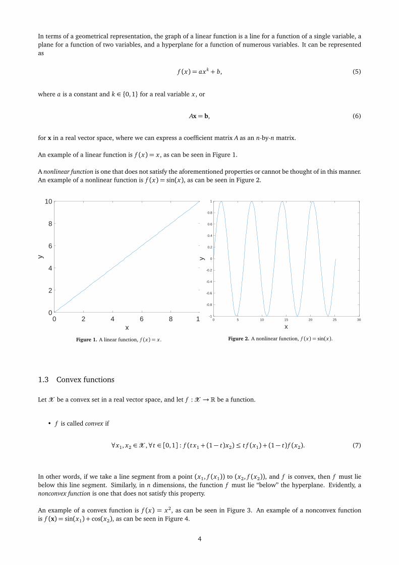
In terms of a geometrical representation, the graph of a linear function is a line for a function of a single variable, aplane for a function of two variables, and a hyperplane for a function of numerous variables. It can be representedas

f (x) = ax k + b, (5)

where a is a constant and k ∈ 0,1 for a real variable x , or

Ax= b, (6)

for x in a real vector space, where we can express a coefficient matrix A as an n-by-n matrix.

An example of a linear function is f (x) = x , as can be seen in Figure 1.

A nonlinear function is one that does not satisfy the aforementioned properties or cannot be thought of in this manner.An example of a nonlinear function is f (x) = sin(x), as can be seen in Figure 2.

0 2 4 6 8 10x

0

2

4

6

8

10

y

Figure 1. A linear function, f (x) = x .

0 5 10 15 20 25 30

x

-1

-0.8

-0.6

-0.4

-0.2

0

0.2

0.4

0.6

0.8

1y

Figure 2. A nonlinear function, f (x) = sin(x).

1.3 Convex functions

Let X be a convex set in a real vector space, and let f :X → R be a function.

• f is called convex if

∀x1, x2 ∈ X ,∀t ∈ [0,1] : f (t x1 + (1− t)x2)≤ t f (x1) + (1− t) f (x2). (7)

In other words, if we take a line segment from a point (x1, f (x1)) to (x2, f (x2)), and f is convex, then f must liebelow this line segment. Similarly, in n dimensions, the function f must lie “below” the hyperplane. Evidently, anonconvex function is one that does not satisfy this property.

An example of a convex function is f (x) = x2, as can be seen in Figure 3. An example of a nonconvex functionis f (x) = sin(x1) + cos(x2), as can be seen in Figure 4.

4

-100 -80 -60 -40 -20 0 20 40 60 80 100

x

0

1000

2000

3000

4000

5000

6000

7000

8000

9000

10000

y

(x1, f(x

1)

(x2, f(x

2)

Figure 3. A convex function, f (x) = x2.

-220

-1.5

-1

-0.5

10 20

0

f(x,

y)

0.5

10

1

y

0

1.5

x

0

2

-10-10

-20 -20

Figure 4. A nonconvex function, f (x) =sin(x1) + cos(x2).

1.4 Nonlinear and nonconvex nature of the problem

Notably, the SCOPF problem is a case of nonlinear programming, i.e., solving an optimization problem defined by asystem of equalities and inequalities, collectively termed constraints, over a set of unknown variables, along with anobjective function to be minimized, where some of the constraints or the objective function are nonlinear [13]. TheSCOPF problem is both nonlinear and nonconvex.

Given the nonlinear nature of the problem, there may be many local optima – an example where we can see that anonlinear problem has many local optima is the aforementioned function f (x) = sin(x), as seen in Figure 2.

In convex optimization, there is a unique optimal solution, which is globally optimal; otherwise, we can prove thatthere is no feasible solution to the problem. Thus, given that the problem is in part nonconvex, we may have morethan one optimal solution, which may not necessarily be globally optimal. Moreover, due to the nonconvex nature ofthe problem, we need to correct properties of the Hessian matrix in order to ensure that the search direction yieldsa decrease in the objective function.

2 Unconstrained Optimization

2.1 Summary

This summary is based on the text published in chapter 9.2 of the book A First Course in Numerical Methods (Ascher,Greif) [7].

In unconstrained optimization, we look at our familiar objective function, f (x), which we wish to minimize, i.e.,we have the following problem:

minimizex∈X f (x), (8)

where we require that the objective function f : X → R be a sufficiently smooth function (in several variables),without constraints.

A necessary condition for a minimum, x∗, of (8) is

∇ f (x∗) = 0, (9)

i.e., we require a vanishing gradient at the point x∗. Generally, a point where the gradient vanishes is called a criticalpoint.

5

The gradient vector, ∇ f (x), is defined as follows:

∇ f (x) =

∂ f∂ x1∂ f∂ x2...∂ f∂ xn

.Furthermore, a sufficient condition for a critical point to be a minimum is that the Hessian matrix ∇2 f (x∗) be sym-metric positive definite. We recall that a matrix A is symmetric if it is a square matrix, i.e., A ∈ Rn×n, and A = AT .Furthermore, we note that a matrix is positive definite if xT Ax> 0 ∀x = 0.

The Hessian matrix, ∇2 f (x), is defined as follows:

H(x) =∇2 f (x) =

∂ 2 f∂ x2

1

∂ 2 f∂ x1∂ x2

. . . ∂ 2 f∂ x1∂ xn

∂ 2 f∂ x2∂ x1

∂ 2 f∂ x2

2. . . ∂ 2 f

∂ x2∂ xn

......

. . ....

∂ 2 f∂ xn∂ x1

∂ 2 f∂ xn∂ x2

. . . ∂ 2 f∂ x2

n

.

We note that in order to satisfy the necessary condition for a minimum, we require that f ∈ C1, i.e., that it is suf-ficiently smooth and differentiable, at least to first order. Moreover, in order to satisfy the sufficient condition for aminimum, we require that f ∈ C2, i.e., that it is sufficiently smooth and differentiable at least to second order.

In general, solving (8) yields n nonlinear equations in n unknowns. For realistic problems, we often cannot findminimum points by inspection. Usually, it is unclear how many local minima a function f (x) has, and if it has morethan one local minimum, how to efficiently find the global minimum, which has the smallest value for f (x).

Furthermore, sometimes there is no finite argument at which a function attains a minimum or a maximum. Forexample, consider f (x) = x2

1 + x22 (Figure 5), which has a unique minimum at the origin (0,0), and no maximum.

Now, consider f (x) = −(x21 + x2

2) (Figure 6), which has a unique maximum at the origin (0,0), and no minimum.

0100

0.5

50 100

1

f(x,

y)

104

50

1.5

y

0

x

0

2

-50-50

-100 -100

Figure 5. f (x) = x21 + x2

2 .

-2100

-1.5

50 100

-1

104

f(x,

y)

50

-0.5

y

0

x

0

0

-50-50

-100 -100

Figure 6. f (x) = −(x21 + x2

2).

As a final note, we recognize that, in general, finding a maximum for f (x) is equivalent to finding the minimumfor − f (x).

3 Constrained Optimization

3.1 Summary

This summary is based on the text published in chapter 9.3 of the book A First Course in Numerical Methods (Ascher,Greif) [8].

6

In essence, we are looking at our familiar objective function, f (x), which we wish to minimize, subject to certainequality and/or inequality constraints, i.e., we have the following problem:

minimizex∈X f(x) (10a)

subject to g(x) = 0, (10b)

h(x)≥ 0, (10c)

xmin ≤ x≤ xmax. (10d)

We recall that g :X →Y and h :X →Z , meaning that g and h may be constructed from various functions gi andhi , respectively. Furthermore, we now group g and h into a single function c, defined as follows:

c(x) =

g(x)h(x)

, (11)

which comprises all equality and inequality constraints — please note that this is not the same as the method of slackvariables which we will discuss later in subsection 3.2. Therefore, we expand the definition of Ω from (3) as follows[8]:

Ω := x ∈ X | ci(x) = 0, i ∈ E , ci(x)≥ 0, i ∈ I . (12)

Hence, E and I are the set of indices corresponding to equality and inequality constraints, respectively. We assumethat ∀i ci(x) ∈ C1. Moreover, we refer to any point x ∈ Ω as a feasible solution, which we note is not necessarily anoptimal solution.

If the unconstrained minimum of f is inside Ω, then we have our basic unconstrained minimization problem, asin section 2. Here, we consider the case where the unconstrained minimizer of f is not inside Ω.

A level set consists of all points x for which f (x) has the same value. Morever, the gradient of f at some point xis orthogonal to the level set that passes through that point.

We define the active set for each x ∈ X as follows:

A (x) := E ∪ i ∈ I | ci(x) = 0. (13)

Hence, we look for solutions whereA (x∗) is nonempty [8].

As in section 2, we have first order necessary and second order necessary and sufficient conditions for a local min-imum. We will only desribe the first order necessary conditions for simplicity. We begin by assuming constraintqualification [8].

Definition 3.1 Constraint qualification Let x∗ be a local critical point and denote by ∇ci(x) the gradients of the con-straints. Furthermore, let AT∗ be the matrix whose columns are the gradients ∇ci(x∗) of all active constraints, i.e., thosebelonging toA (x∗). The constraint qualitication assumption is that AT∗ has full column rank.

Now, let us define the LagrangianL (x,λ) = f (x)− ∑

i∈E∪Iλici(x). (14)

Then, we have the following necessary first order conditions for a minimum, collectively known as the Karush–Kuhn–Tucker (KKT) conditions [8]:

Theorem 3.1 Constrained Minimization Conditions. Assume that f (x) and ci(x) are smooth enough near a criticalpoint x∗ and that constraint qualification holds. Then there is a vector of Lagrange multipliers λ∗ such that

∇xL (x∗,λ∗) = 0, (15a)

ci(x∗) = 0 ∀i ∈ E , (15b)

ci(x∗)≥ 0 ∀i ∈ I , (15c)

λ∗i ≥ 0 ∀i ∈ I , (15d)

λ∗i ci(x∗) = 0 ∀i ∈ E ∪I . (15e)

7

Moreover, we have

∇L(x,λ) =

∇x L(x,λ)∇λL(x,λ)

=

∇ f (x)−∇cT(x)λ−c(x)

, (16a)

∇2 L(x,λ) =

∇xx L(x,λ) ∇xλL(x,λ)∇λx L(x,λ) ∇λλL(x,λ)

=

∇2 f (x)−∇2c(x)λ −∇cT(x)−∇c(x) 0

, (16b)

where we refer to H(x) =∇2 f (x) as the Hessian of f (x), and J(x) =∇c(x) as the Jacobian of the constraints.

The Hessian has the following structure:

H(x) =

∂ 2 f∂ x2

1

∂ 2 f∂ x1∂ x2

. . . ∂ 2 f∂ x1∂ xn

∂ 2 f∂ x2∂ x1

∂ 2 f∂ x2

2. . . ∂ 2 f

∂ x2∂ xn

......

......

∂ 2 f∂ xn∂ x1

∂ 2 f∂ xn∂ x2

. . . ∂ 2 f∂ x2

n

. (17)

The Jacobian has the following structure:

J(x) =

∂ c1∂ x1

∂ c1∂ x2

. . . ∂ c1∂ xn

∂ c2∂ x1

∂ c2∂ x2

. . . ∂ c2∂ xn

......

......

∂ cm∂ x1

∂ cm∂ x2

. . . ∂ cm∂ xn

. (18)

We revisit our examples of unconstrained minimization from Figure 5 and Figure 6, but with the addition of con-straints on the variables x1 and x2. Thus, we have the following examples for constrained optimization

minimizex∈R2

x21 + x2, (19a)

subject to x21 + x2

2 ≤ r2. (19b)

maximizex∈R2

− (x21 + x2), (20a)

subject to x21 + x2

2 ≤ r2. (20b)

We set r = 100, with Figure 7 corresponding to (19), and with Figure 8 corresponding to (20).

0100

0.5

50 100

1

104

f(x,

y)

50

1.5

y

0

x

0

2

-50-50

-100 -100

Figure 7. f (x) = x21 + x2

2 .

-2100

-1.5

50 100

-1

104

f(x,

y)

50

-0.5

y

0

x

0

0

-50-50

-100 -100

Figure 8. f (x) = −(x21 + x2

2).

3.2 Slack variables

We can convert inequality constraints to equality constraints by introducing slack variables, i.e.,

ci(x) = 0 for i ∈ E , (21a)

ci(x)− s= 0 for i ∈ I , (21b)

s≥ 0, s ∈ Rm, (21c)

xmin ≤ x≤ xmax, xmin,xmax ∈ Rn. (21d)

8

Hence, we define

xS =

xs

, (22a)

g(x) := ci(x), for i ∈ E , (22b)

h(x, s) := ci(x)− s, for i ∈ I . (22c)

and solve for the following:

minimizexS∈X

f(xS) (23a)

subject to

g(x)

h(x, s)

=

00

, (23b)

xmin ≤ x≤ xmax, (23c)

s≥ 0. (23d)

4 Primal-Dual Interior Point Method

This summary is based on the text published in thesis [15].

4.1 Summary

The system of equations formed in (1) yield a problem that is nonlinear and nonconvex. Such a problem leads us toa nonlinear program (NLP), i.e., the process of solving an optimization problem defined by a system of equalities andinequalities — collectively termed constraints — over a set of unknown variables, along with an objective functionto be maximized or minimized, where some of the constraints of the objective function are nonlinear [13].

For simplicity, let us consider the following NLP:

minimizex∈X f(x) (24a)

subject to c(x) = 0 (24b)

x (i) ≥ 0, (24c)

where x (i) denotes the ith element of x.

A popular class of algorithms used to solve NLPs are called sequential quadratic programming (SQP) methods. Un-fortunately, at the beginning of the optimization process these type of methods may require a considerable amountof time to identify the active set A , a problem that is known to be an NP-hard combinatorial problem. Thus, in theworst case, the solution time increases exponentially with the size of the problem.

4.2 Barrier methods

There exist methods that can get around the problem of identifying the active bound constraints mentioned in subsec-tion 4.1. Such a class of methods are barrier methods; they circumvent the problem by replacing the bound constraintswith a logarithmic barrier term which is added to the objective function f . For now, we assume that there are noinequality constraints other than the bounds (24c). We can make this assumption given that, using slack variables,we convert inequality constraints to equality constraints and are left only with the bounds on the variables x and s,as illustrated in (23). Thus, we have the following problem:

minimizex∈X ϕµ(x) := f (x)−µ∑

i∈Ilnx (i), (25a)

subject to c(x) = 0, (25b)

where µ is the barrier parameter, subject to µ > 0. We recall that the ln(x) function is not defined at x = 0.

9

Hence, the objective function of our barrier problem (25) becomes increasingly large as x approaches the bound-ary of the region, defined by the lower bounds (24c). Therefore, the solution xµ∗ must lie in the interior of this set,i.e., (xµ∗ )(i) > 0 for i ∈ I .

The degree of influence of the barrier term “−µ∑i∈I ” is determined by the size of µ and, under certain condi-tions, xµ∗ converges to a local solution x∗ of the original problem (24) as µ→ 0.

The KKT conditions for our system (25) are thus:

∇ϕµ(x) +∇c(x)Tλ= 0, (26a)

c(x) = 0. (26b)

Solving this system of equations directly with a Newton-type method, as in a straightforward application of an SQPmethod to (25), leads to a method we refer to as a primal method, which deals only with the primal variables x andpossibly the equality multipliers λ as iterates. However, the term “∇ϕµ(x)” has components including µ

x (i) , thus,the system is not defined at a solution x∗ of our base NLP (24) with the active bound x (i) = 0, and the radius ofconvergence of Newton’s method applied to (26) converges to 0 as µ→ 0, i.e., there are increasingly fewer startingpoints for which the method converges.

For this reason, it is sometimes more suitable to use primal-dual methods rather than following a primal approach.Here, we introduce the dual variables v, defined as:

v(i) :=µ

x (i). (27)

With this definition, the KKT conditions (26) are quivalent to the following perturbed KKT conditions or primal-dualequations:

∇ϕµ(x) +∇c(x)Tλ− v= 0, (28a)

c(x) = 0, (28b)

x (i)v(i) −µ= 0 for i ∈ I . (28c)

We notice that for µ= 0, the conditions (28) together with the inequalities

x (i) ≥ 0 and v i ≥ 0 for i ∈ I (29)

are actually the KKT conditions (26) for the barrier problem (25), where the dual variables v then correspond to themultipliers for the bound constraints (24c).

Primal-dual methods solve system (28) using a Newton-type approach, maintaining iterates for both xk and vk,and possibly λk. Since the inequalities (29) hold strictly at the optimal solution of the barrier problem (25) forµ > 0, xk and vk are always required to strictly satisfy the inequalities, i.e.,

x (i)k > 0 and v(i)k > 0 for i ∈ I (30)

for all k, and can approach 0 only asymptotically as µ→ 0. Given that the bound 0 is never actually reached, thesemethods are often called interior point methods.

An example of how such a method works in R2 can be seen in Figure 9 — blue lines show the constraints, redshows each iteration of the algorithm [5].

10

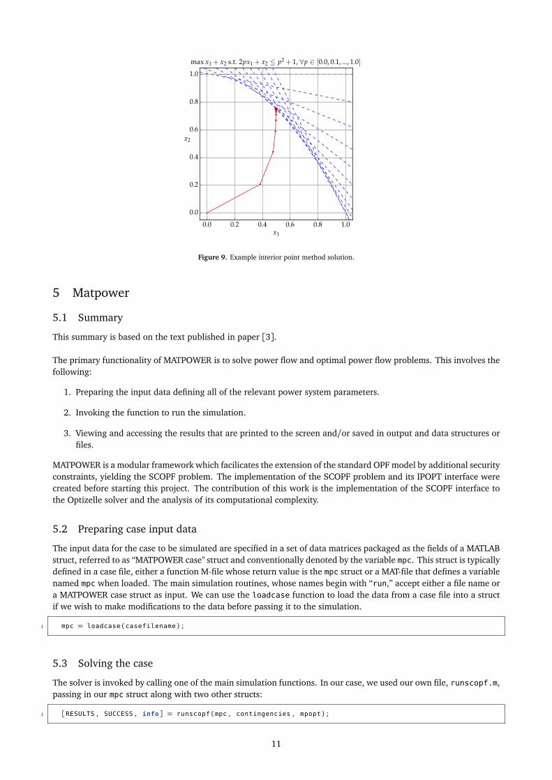
Figure 9. Example interior point method solution.

5 Matpower

5.1 Summary

This summary is based on the text published in paper [3].

The primary functionality of MATPOWER is to solve power flow and optimal power flow problems. This involves thefollowing:

1. Preparing the input data defining all of the relevant power system parameters.

2. Invoking the function to run the simulation.

3. Viewing and accessing the results that are printed to the screen and/or saved in output and data structures orfiles.

MATPOWER is a modular framework which facilicates the extension of the standard OPF model by additional securityconstraints, yielding the SCOPF problem. The implementation of the SCOPF problem and its IPOPT interface werecreated before starting this project. The contribution of this work is the implementation of the SCOPF interface tothe Optizelle solver and the analysis of its computational complexity.

5.2 Preparing case input data

The input data for the case to be simulated are specified in a set of data matrices packaged as the fields of a MATLABstruct, referred to as “MATPOWER case" struct and conventionally denoted by the variable mpc. This struct is typicallydefined in a case file, either a function M-file whose return value is the mpc struct or a MAT-file that defines a variablenamed mpc when loaded. The main simulation routines, whose names begin with “run,” accept either a file name ora MATPOWER case struct as input. We can use the loadcase function to load the data from a case file into a structif we wish to make modifications to the data before passing it to the simulation.

1 mpc = loadcase (casefilename ) ;

5.3 Solving the case

The solver is invoked by calling one of the main simulation functions. In our case, we used our own file, runscopf.m,passing in our mpc struct along with two other structs:

1 [RESULTS , SUCCESS , info ] = runscopf (mpc , contingencies , mpopt ) ;

11

Where mpc is as aforementined, contingencies is our contingency set, and mpopt is a struct containing MATPOWERoptions.

Finally, in order to extract the results, we can simply access the RESULTS struct. Moreover, if we’re looking forinformation, such as the time taken to execute the algorithm, we can extract it from the info struct. In essence,we can choose which information we want to deliver back to the user from our solvers; in fact, this flexibility wasexploited and it is how we put the results together. We note that in case of failure, these results are not deliveredback to the user, as an exception is thrown.

6 Optimization Software

In section 5, we gave a high-level description of how MATPOWER can be set up and used to solve the OPF or theSCOPF problem. However, we have yet to explore how we set up the IPOPT and Optizelle solvers that were used byMATPOWER to solve the problem.

6.1 IPOPT

This summary is based on the text published in paper [1], and the text published in the website for IPOPT [14].

6.1.1 Introduction to IPOPT

IPOPT (Interior Point OPTimizer, pronounced eye-pea-Opt) is a software package for large-scale nonlinear optimiza-tion. It is designed to find (local) solutions of mathematical optimization problems of the following form:

minimizex∈Rn

f (x) (31a)

subject to cmin ≤ c(x)≤ cmax, (31b)

xmin ≤ x≤ xmax, (31c)

where f (x) : Rn→ R is the objective function, and c(x) : Rn→ Rm are the constraint functions, which comprise bothequality and inequality constraints. The vectors cmin and cmax denote the lower and upper bounds on the constraints,and the vectors xmin and xmax are the bounds on the variables x. The functions f (x) and c(x) can be nonlinear andnonconvex, but should be twice continuously differentiable (C2) [14]. Indeed, we require C2 in order to satisfy thesufficient condition for a minimum. We note that, where we wish to express equality constraints, we would set thecorresponding components in cmin and cmax to the same value.

IPOPT is written in C++ and is released as open source code under the Eclipse Public License (EPL). It is avail-able from the COIN-OR initiative [4].

The IPOPT distribution can be used to generate a library linked to one’s own C++, C, Fortran, or Java code, aswell as a solver executable for the AMPL [11]modeling environment. The package includes interfaces to CUTEr [12]optimization testing environment, as well as the MATLAB and R programming environments. IPOPT can be used onLinux/UNIX, Mac OS X, and Windows platforms.

Some special features of IPOPT are [14] the following:

• Derivative checker.

• Hessian approximation.

• Warm starts via AMPL.

• Ipopt: Optimal Sensitivity Based on AMPL/Ipopt.

• Employing second derivative information, if available, or otherwise approximating it by means of a limited-memory quasi-Newton approach (BFGS and SR1) [2].

• Global convergence of the method is ensured by a line search procedure, based on a filter method [2].

One drawback of IPOPT is that it is not thread-safe; it currently uses smart pointers and a tagging mechanism [2].

12

6.1.2 Interfacing with IPOPT through code

IPOPT requires more than the problem definition, namely, the following:

1. Problem dimensions.

• Number of variables.

• Number of constraints.

2. Problem bounds.

• Variable bounds.

• Constraint bounds.

3. Initial starting point.

• Initial values for the primal x variables.

• Initial values for the multipliers (only required for warm-start option).

4. Problem structure.

• Number of nonzeros in the Jacobian of the constraints.

• Number of nonzeros in the Hessian of the Lagrangian function.

• Sparsity structure of the Jacobian of the constraints.

• Sparsity structure of the Hessian of the Lagrangian function.

5. Evaluation of problem functions — information evaluated using a given point (x,λ,σ f ), coming from IPOPT.

• Objective function f (x).

• Gradient of the objective ∇ f (x).

• Constraint function values c(x).

• Jacobian ∇c(x)T of the constraints.

• Hessian of the Lagrangian function, L(x,λ), where,

L(x,λ) = f (x) + ⟨c(x),λ⟩, (32)

Hxx(x,λ,σ f ) = σ f∇2 f (x) + ⟨∇2c(x),λ⟩, (33)

where we introduce a factor σ f in front of the objective term so that IPOPT can ask for the Hessian ofthe objective function or the constraints independently, if required. We could choose only the objectiveterm by setting the constraint multipliers λi to 0 and σ f to 1. Evidently, to choose only the constraints,we would set σ f to 0.

Moreover, we note that IPOPT is invoked as follows:

1 [x , info ] = ipopt (x0 , funcs , options ) ;

Here:

• x0 is our initial guess.

• funcs is a struct that containts the definitions of the following:

– The objective function: f (x).

– The gradient of the objective function: ∇ f (x).

– The evaluation of the constraints: c(x).

– The Jacobian of the constraints: ∇c(x).

– The Hessian of the Lagrangian function (see (33)).

– The structure of the Jacobian of the constraints.

13

– The structure of the Hessian of the Lagrangian function.

• options is a struct that contains the following:

– (Possibly) auxiliary data.

– Options for the interior point method.

– Lower and upper bounds for the primal variables x.

– Lower and upper bounds for the constraints ci(x).

– (Optional, for warm start) Set initial values for the Lagrange multipliers for the lower and upper bounds onthe variables and for the constraints. A warm start is enabled by setting the option warm_start_init_point

= ’yes’.

In the remainder of this section, we go deeper into the requirements from IPOPT and show some code excerpts whereappropriate.

6.1.3 Problem dimension

In the context of our problem, what is meant by the problem dimension is the number of variables x i that make upthe vector of unknown variables x, as well as the number of constraints in our problem, i.e., the number of constraintsci(x) together with the bounds xmin < x < xmax discussed in (10). We note that there is no need to formulate theproblem using slack variables as presented in subsection 3.2 in IPOPT, as the problem is automatically formulated as(2) [15]. Moreover, the number of variables and the number of constraints are derived automatically by IPOPT.

6.1.4 Problem bounds

The problem bounds in IPOPT consist of the bounds on the variable x and the bounds on the equality and inequalityconstraints. We note that the equality and inequality constraints are grouped together in c(x). Hence, we are referringspecifically to the following:

minimizex∈Rn

f (x) (34a)

subject to cmin ≤ c(x)≤ cmax, (34b)

xmin ≤ x≤ xmax. (34c)

As we know from our standard problem formulation (1), we don’t have upper bounds on the equality and inequalityconstraints, we only have lower bounds. In IPOPT, the concept of being unbounded from above is, by definition,+∞. Hence, we have the following:

minimizex∈Rn

f (x) (35a)

subject to cmin ≤ c(x)≤ +∞, (35b)

xmin ≤ x≤ xmax. (35c)

In the code, we need to specify the bounds individually for each x i and each ci , respectively; however, we can groupthe individual bounds in an array. Furthermore, we need to specify the bounds separately for the variables and theconstraints. Here is an excerpt from the code that illustrates how this was done:

1 options . lb = xmin ;2 options . ub = xmax ;3 options . cl = [repmat ( [ zeros ( 2 nb , 1) ; −Inf ( 2 nl2 , 1) ] , [ns , 1]) ; l ] ;4 options . cu = [repmat ( [ zeros ( 2 nb , 1) ; zeros ( 2 nl2 , 1) ] , [ns , 1]) ; u+1e10 ] ;

Here options.lb and options.ub denote the lower and upper bounds on x, respectively, and options.cl andoptions.cu denote the lower and upper bounds on c(x), respectively.

As was mentioned in section 1, nb represents the number of buses, and though not previously mentioned, nl2 de-notes the number of constrained lines. The MATLAB function repmat allows us to repeat the lower and upper boundson the constraints for each scenario. This can be seen as the bounds are repeated ns times, where ns represents thenumber of scenarios.

As also previously mentioned in section 1, we recall that the bounds on x already account for all scenarios, since

14

x contains variables for all scenarios as well as global variables required for the optimization.

Furthermore, we defined xmin and xmax in the previous code excerpt using the MATPOWER package and later madesome modifications in the code so that the bounds aligned with our SCOPF problem. This was done as follows:

1 %% bounds on optimization vars xmin <= x <= xmax

2 [x0 , xmin , xmax ] = getv (om ) ; %returns standard OPF form [Va Vm Pg Qg]

3

4 % add small pertubation to UB so that we prevent ipopt removing variables

5 % for which LB=UB, except the Va of the reference bus

6 tmp = xmax (REFbus_idx ) ;7 xmax = xmax + 1e−10;8 xmax (REFbus_idx ) = tmp ;9

10 % replicate bounds for all scenarios and append global limits

11 xl = xmin ( [ VAopf VMopf (nPVbus_idx ) QGopf PGopf (REFgen_idx ) ] ) ; %local variables

12 xg = xmin ( [ VMopf (PVbus_idx ) PGopf (nREFgen_idx ) ] ) ; %global variables

13 xmin = [repmat (xl , [ns , 1]) ; xg ] ;14

15 xl = xmax ( [ VAopf VMopf (nPVbus_idx ) QGopf PGopf (REFgen_idx ) ] ) ; %local variables

16 xg = xmax ( [ VMopf (PVbus_idx ) PGopf (nREFgen_idx ) ] ) ; %global variables

17 xmax = [repmat (xl , [ns , 1]) ; xg ] ;

6.1.5 Initial starting point

Given that we did not use the warm-start option for IPOPT, we only needed to specify the initial values for the primalvariables x, i.e., as described in 6.1.2, we only need to specify our initial guess x0. We note that in the code, x0 wasfirst defined using the MATPOWER package, as shown in the previous code excerpt, but was later modified in anattempt to select an interior initial point based on the bounds, as follows:

1 ll = xmin ; uu = xmax ;2 ll (xmin == −Inf ) = −1e10 ; %% replace Inf with numerical proxies

3 uu (xmax == Inf ) = 1e10 ;4 x0 = (ll + uu ) / 2; %% set x0 mid-way between bounds

5 k = find (xmin == −Inf & xmax < Inf ) ; %% if only bounded above

6 x0 (k ) = xmax (k ) − 1; %% set just below upper bound

7 k = find (xmin > −Inf & xmax == Inf ) ; %% if only bounded below

8 x0 (k ) = xmin (k ) + 1; %% set just above lower bound

9

10 % adjust voltage angles to match reference bus

11 Varefs = bus (REFbus_idx , VA ) (pi/180) ;12 for i = 0:ns−113 idx = model . index . getGlobalIndices (mpc , ns , i ) ;14 x0 (idx (VAscopf ) ) = Varefs (1) ;15 end

6.1.6 Problem structure

As we have discussed before, IPOPT needs to know the number of nonzeros in both the Jacobian of the constraints,∇c(x), and the Hessian of the Lagrangian function. This, however, can be derived by IPOPT as soon as we define thesparsity structure of both.

In order to specify the sparsity structure of the Jacobian of the constraints and the Hessian of the Lagrangian func-tion for our SCOPF problem, a relatively large portion of code was used. For the interested reader, you can find thisportion of code in Appendix A.

6.1.7 Evaluation of problem functions

As mentioned before, in order to call IPOPT we require a funcs structure. This structure contains all of the functionsthat we need in order to evaluate the problem functions using a given point (x,λ,σ f ), kept by IPOPT. In the code,we defined the funcs structure as follows:

1 %% assign function handles

2 funcs . objective = @objective ;3 funcs . gradient = @gradient ;4 funcs . constraints = @constraints ;

15

5 funcs . jacobian = @jacobian ;6 funcs . hessian = @hessian ;7 funcs . jacobianstructure = @ (d ) Js ;8 funcs . hessianstructure = @ (d ) Hs ;

Here the function handles correspond to the definitions of the functions mentioned in 6.1.2. For the interested reader,you can find the portions of the code to define these functions in Appendix A.

6.1.8 Pros and cons

Pros:

• The problem dimensions and bounds come solely from the problem definition.

• It is a nonlinear programming solver designed for solving sparse large-scale problems.

• It can be customized for a variety of matrix formats (for instance, triplet format) [14].

Cons:

• It needs to know the number of nonzero elements and the sparsity structure (row and column indices of eachof the nonzero entries) of the constraint Jacobian and the Hessian of the Lagrangian function.

– Once defined, this nonzero structure must remain constant for the entire optimization procedure, meaningthat the structure needs to include entries for any element that could ever be nonzero, not only those thatare nonzero at the starting point.

6.2 Optizelle

This summary is based on the text published in the manual of Optizelle (version 1.2.0) [17], and the text publishedin the website for Optizelle [16].

6.2.1 Introduction to Optizelle

Optizelle is an open source software library designed to solve general purpose nonlinear optimization problems of thefollowing form(s):

• Unconstrained

minimizex∈X f (x). (36a)

• Equality constrained


subject to g(x) = 0. (37b)

• Inequality constrained


subject to h(x)≥ 0. (38b)

• Constrained



h(x)≥ 0. (39c)

It features the following:

• State of the art algorithms:

16

– Unconstrained — steepest descent, preconditioner nonlinear-CG (Fletcher–Reeves, Polak–Ribiere, Hestenes–Stiefel), BFGS, Newton-CG, SR1, trust-region Newton, Barzilai–Borwein two point approximation.

– Equality constrained — inexact composite-step SQP.

– Inequality constrained — primal-dual interior point method for cone constraints (linear, second-order cone,and semidefinite), log-barrier method for cone constraints.

– Constrained — any combination of the above.

• Open source:

– Released under the 2-Clause BSD License.

– Free and ready to use with both open and closed source commercial codes.

• Multilanguage support:

– Interfaces to C++, MATLAB/Octave, and Python.

• Robust combinations and repeatability:

– Can stop, archive, and restart the computation from any optimization iteration.

– Combined with multilanguage support, the optimization can be started in one language and migrated toanother.

• User-defined parallelism:

– Fully compatible with OpenMP, MPI, and GPUs.

• Extensible linear algebra:

– Supports user-defined vector algebra and preconditioners.

– Enables sparse, dense, and matrix-free computations.

– Defines custom inner products and compatibility with preconditioners such as algebraic multigrid whichmakes Optizelle well-suited for PDE constrained optimization.

• Sophisticated control of the optimization algorithms:

– Allows the user to insert arbitrary code into the optimization algorithm, which enables custom heuristicsto be embedded without modifying the source.

Furthermore, there is a community forum for Optizelle.

In our experience, one drawback for Optizelle is that the documentation [17] stated that the inequality constraintscould be formulated as follows:

h(x)≥ 0;

however, we observed that strict inequalities h(x)> 0 were required; otherwise, problems would arise in solving theSCOPF problem. Our observation seems to have been confirmed in the forum post found in [18].

6.2.2 Interfacing with Optizelle through code

As was mentioned before in section 1, we have

• f :X → R is the objective function we wish to minimize,

• g :X →Y are the equality constraints,

• h :X →Z are the inequality constraints,

where X , Y , and Z denote vector spaces, more specifically, Hilbert spaces [17]. For our problem, these vectors spacesare in Rm, but Optizelle allows for the vector spaces to be spaces of functions such as L2(Ω) or matrices such as Rm×n

as long as one provides the necessary operations required to compute on a vector of such a vector space [17].

Other than this, in order solve our NLP, Optizelle requires for us to define the following:

17

• The objective function f (x), the gradient of the objective function ∇ f (x), and the Hessian of the objectivefunction ∇2 f (x).

• The equality constraints, which are encoded into a function g(x) , the Jacobian of the equality constraints∇g(x), and the Hessian of the equality constraints ∇2g(x).

• The inequality constraints, which are encoded into a function h(x), the Jacobian of the inequality constraints∇h(x), and the Hessian of the inequality constraints ∇2h(x).

Indeed, the Hessian definitions are necessary if we wish to use second-order algorithms.

It is important to note that Optizelle allows for the equality constraints to be nonlinear, but it requires that the inequal-ity constraints be affine [17]. We recall an affine function is one where ∀α ∈ R, h(αx+(1−α)x) = αh(x)+(1−α)h(x)or, equivalently, h′′(x) = 0. This is required in order to simplify the line search that maintains the nonnegativity ofthe inequality constraints. In our SCOPF problem, we have a basis consisting of nonlinear equality and inequalityconstraints. For this reason, our original problem formulation (1) (repeated here for clarity):



h(x)≥ 0, (40c)

xmin ≤ x≤ xmax, (40d)

was reformulated as follows, using slack variables:


subject to

g(x)

h(x)− s

=

00

, (41b)

s≥ 0, (41c)

xmin ≤ x≤ xmax. (41d)

In order to optimize effectively, Optizelle requires the evaluation cε(x, s) :=

g(x)

h(x)− s

, the Fréchet (total) derivative

applied to a vector, c′ε(x, s)δx, and the adjoint of the Fréchet derivative applied to the vector of Lagrange multipliersfor the equality constraints, c′ε(x, s)δy. In order to use second-order algorithms, we also require the second derivativeoperation (c′′ε (x, s)δx)δy.

Let us define the reformulated inequality constraints as

cι(x, s) :=

xmin ≤ x≤ xmax

s≥ 0

. (42)

As was the case for the (reformulated) equality constraints cε(x, s), we require the same operations from cι(x, s) butsince cι(x, s) is affine, (c′′ι (x, s)δx)δz= 0.

6.2.3 Setting up Optizelle

To start, we need to create an optimization state, which contains an entire description of the current state of theoptimization algorithm. This is unique to the particular optimization problem, but all algorithms in a particularformulation share the same state [17]. Most algorithms do not require information about all of these pieces, butthey are present to make it easier to switch from one algorithm to another. In order to define an optimization state,we instantiate the state class with the particular class of formulation we need. In our case, we have a constrainedoptimization problem, so we define the optimization state by

1 state = Optizelle . Constrained . State . t (X , Y , Z , x , y , z ) ;

Here, X, Y, and Z are the vector spaces corresponding to the codomain of our functions f , g, and h, respectively, fromour standard formulation (1). In our case, X , Y, Z ∈ Rm. We note that in the remainder of this section, x correspondsto xS (compare (22a)), with the slack variables initialized to s= 0+ε, where ε represents a small perturbation whichwas required based on our observation that the inequality constraints cι needed to be strictly satisfied. In the code

18

excerpt above, x≡ xS , y, and z denote the initial guesses for our unknown primal variables x, the equality multipliersy, and the inequality multipliers z, respectively.

In order to pass the functions used in the optimization to Optizelle, we accumulate each of them into a bundle of func-tions. These bundles are simple structures that contain the appropriate function. Given that we have a constrainedproblem, we define this as follows:

1 fns = Optizelle . Constrained . Functions . t ;

Then, we can define the information related to our objective function f (x), our equality constraints g(x), and ourinequality constraints h(x) as follows:

1 fns . f = MyObj (myauxdata ) ;2 fns . g = MyEq (myauxdata ) ;3 fns . h = MyIneq (myauxdata ) ;

where myauxdata contains information that is used locally in each of the function evaluations.

In the following code excerpts, we show how we defined the functions used by Optizelle at a high level:

1 %% Define objective function.

2 function self = MyObj (myauxdata )3 % Evaluation

4 self . eval = @ (x ) objective (x , myauxdata ) ;5

6 % Gradient

7 self . grad = @ (x ) gradient (x , myauxdata ) ;8

9 % Hessian-vector product

10 self . hessvec = @ (x , dx ) hessvec (x , dx , myauxdata ) ;11 . . .12 end

In order to optimize the objective function f (x), Optizelle requires for us to provide the evaluation of the objectivefunction, and the gradient of the objective function. In order to use second-order algorithms, we also need to providethe product of the Hessian of the objective function with a vector δx . In the code excerpt above, we return astruct containing all of these necessary components, i.e., the returned struct self. Above, self is composed of thefollowing:

• self.eval is defined as the function handle to our function which evaluates f (x).

• self.grad is defined as the function handle to our function which evaluates ∇ f (x).

• self.hessvec is defined as the function handle to our function which evaluates ∇2 f (x)δx.

As Optizelle optimizes the objective function f (x), these function handles are called with actual arguments. We willspare the definition of our functions pointed to by the function handles as it is not necessary in order to understandthe code at a high level. For the interested reader, the definition of these functions can be found in Appendix B.

1 %% Define equality constraints.

2 function self = MyEq (myauxdata )3

4 % y=g(x)

5 self . eval = @ (x ) constraints (x , myauxdata ) ;6

7 % y=g’(x)dx

8 self . p = @ (x , dx ) jacobvec (x , dx , myauxdata ) ;9

10 % xhat=g’(x)*dy

11 self . ps = @ (x , dy ) jacobvec (x , dy , myauxdata ) ;12

13 % xhat=(g’’(x)dx)*dy

14 self . pps = @ (x , dx , dy ) hessian (x , myauxdata , dy ) dx ;15 . . .16 end

Similarly to the code excerpt describing the necessary information for the objective function, the code excerpt abovedetails the necessary information for the equality constraints g(x). Here, the returned struct self is composed of thefollowing:

19

• self.eval is defined as the function handle to our function which evaluates g(x).

• self.p is defined as the function handle to our function which evaluates ∇g(x)δx .

• self.ps is defined as the function handle to our function which evaluates ∇g(x) ·δ y .

• self.pps is defined as the function handle to our function which evaluates (∇2g(x)δx) ·δ y .

1 %% Define inequality constraints.

2 function self = MyIneq (myauxdata )3 % z=h(x)


6 % z=h’(x)dx


9 % xhat=h’(x)*dz

10 self . ps = @ (x , dz ) jacobvec (x , dz , myauxdata ) ;11

12 % xhat=(h’’(x)dx)*dz

13 self . pps = @ (x , dx , dz ) sparse (length (x ) , length (x ) ) ;14 . . .15 end

Finally, the code excerpt above details the necessary information for the inequality constraints h(x). Here, the re-turned struct self is composed of the following:

• self.eval is defined as the function handle to our function which evaluates h(x).

• self.p is defined as the function handle to our function which evaluates ∇h(x)δx .

• self.ps is defined as the function handle to our function which evaluates ∇h(x) ·δz.

• self.pps is defined as a sparse zero-matrix, since the inequality constraints are affine.

The last step is for us to call the optimization solver. We note that this can only be done once the state, (optionally)parameters, and functions are set. Given that we have a constrained problem, we invoke Optizelle’s optimizationalgorithm as follows:

1 state = Optizelle . Constrained . Algorithms . getMin ( . . .2 Optizelle . Rm , Optizelle . Rm , Optizelle . Rm , Optizelle . Messaging . stdout , . . .3 fns , state ) ;

After the optimization solver concludes, the solution lives in the optimization state in a variable called x, and thereason the optimization stopped resides in a variable called opt_stop. In the code, we extracted both as follows:

1 % Print out the reason for convergence

2 fprintf (’The algorithm converged due to: %s\n’ , . . .3 Optizelle . OptimizationStop . to_string (state . opt_stop ) ) ;4

5 results = struct (’x’ , state . x ) ;

6.2.4 Pros and cons

Pros:

• Does not need sparsity structure of Jacobian of constraints or Hessian of the Lagrangian function.

• The Lagrangian function does not need to be specified by the user. This means that the user can specify allrelated data to the objective function f (x), the equality constraints g(x), and the inequality constraints h(x),separately; indeed, it is required for the formulation to be done as such. This feature could be viewed favourablywith respect to modularity.

Cons:

• Requires that the inequality constraints function h be affine. Since the equality and inequality constraints inthe SCOPF problem are nonlinear, we are required to reformulate the standard formulation (1) using slackvariables, yielding the formulation (2).

• Being required to separately specify all related data for the objective function f (x), the equality constraintsg(x), and the inequality constraints h(x), means that we have more possible points of failure.

20

7 Experiments

7.1 Methodology

We tested the relative performance of IPOPT and Optizelle by having them solve a SCOPF problem with a growingdynamic contingency set. This means we used a test power grid provided by MATPOWER and identified a feasibledynamic contingency set G . The test power grid we used was case9. We began by testing the frameworks with anempty contingency set — i.e., |G | = 0 — sequentially incrementing the number of contingencies, reaching a maxi-mum of six contingencies — i.e., |G |= 6.

The experiment measured the convergence behaviour of IPOPT and Optizelle by examining the value of the objectivefunction, f (x), the norm of the gradient, ∥∇ f (x)∥, and the value of the power flow equations, g(x). Furthermore,the average time per iteration was measured for both frameworks.

When performing these measurements, no limit on the number of iterations was placed on IPOPT, whereas we limitedthe number of iterations in Optizelle. This was done since IPOPT always managed to converge to a solution in lessthan fifteen iterations, while Optizelle never managed to converge to a solution. In order to measure the averagenumber of iterations for both solvers, the average time and the average number of iterations to reach a stopping pointwas measured — in IPOPT’s case due to convergence to a solution, in Optizelle’s case due to a stopping conditionbeing met. These averages were taken over the results from five repetitions of the experiment.

7.2 The experiment

These were the settings we used for IPOPT in the experiment:

1 print_level 5

2 print_timing_statistics yes

3 linear_solver pardiso

4 pardiso_matching_strategy complete2x2

5 dual_inf_tol 1e-6

6 compl_inf_tol 1e-6

7 constr_viol_tol 1e-6

8 mu_strategy monotone

These were the settings we used for Optizelle in the experiment:

1 "Optizelle" :

2 "msg_level" : 1,

3 "H_type" : "UserDefined",

4 "iter_max" : 5000,

5 "delta" : 100,

6 "eps_trunc" : 1e-6,

7 "eps_grad" : 1e-6,

8 "eps_kind" : "Absolute",

9 "eps_dx" : 1e-6,

10 "Naturals" :

11 "iter" : 14

12

13

although, when measuring the average number of iterations, we set the maximum number of iterations to fifty.

We note that all tolerance values were set to 10−6, for both IPOPT and Optizelle. In particular, we set the toler-ance of the power flow equations to 10−2.

On one hand, in all cases, Optizelle did not converge to a solution that satisfied the power flow equations. Onthe other hand, in all cases, IPOPT converged to a solution that satisfied the power flow equations; moreover, IPOPTtook at most fourteen iterations to converge to a valid solution. From this, we can conclude that IPOPT is both fasterand more accurate than Optizelle. Indeed, this seems to indicate that the implementation of the primal-dual interior

21

point method by IPOPT is more performant and robust than that of Optizelle.

Table 1 lists important details we noticed when trying to solve case9 with different contingency sets (cont, G ),using Optizelle (we note that PF stands for power flow):

Contingency set Maximum PF error Reason for convergencecont = no contingencies 4.618512× 10−1 MaxItersExceededcont = 2 4.013213 MaxItersExceededcont = (2,3) 1.549788 StepSmallcont = (2,3,5) 1.549788 StepSmallcont = (2,3,5,6) 1.549788 StepSmallcont = (2,3,5,6,8) 1.549787 StepSmallcont = (2,3,5,6,8,9) 1.549786 StepSmall

Table 1. Optizelle power flow equation evaluation.

where “StepSmall” indicates that Optizelle converged to a solution that satisfied our setting εdx = 10−6. We notethat in the context of our SCOPF problem, the violation of the power flow equations was significant.

For comparison, we list the maximum PF error from IPOPT in Table 2 below:

Contingency set Maximum PF error Reason for convergencecont = no contingencies 2.9370950116458516× 10−13 Optimal Solution Foundcont = 2 5.6760982025672035× 10−10 Optimal Solution Foundcont = (2,3) 5.7509247364251337× 10−10 Optimal Solution Foundcont = (2,3,5) 2.7187258000438419× 10−10 Optimal Solution Foundcont = (2,3,5,6) 5.6067400722170646× 10−10 Optimal Solution Foundcont = (2,3,5,6,8) 2.4691740763138625× 10−7 Optimal Solution Foundcont = (2,3,5,6,8,9) 9.6350508127507339× 10−10 Optimal Solution Found

Table 2. IPOPT power flow equation evaluation.

Comparing the results from Table 1 and Table 2, we have further proof that IPOPT not only performed better thanOptizelle, but it performed better than we required it to. Indeed, the highest evaluation of the constraints by IPOPTwas 2.4691740763138625×10−7, which is five orders of magnitude more accurate than required by our power flowequations tolerance value of 10−2.

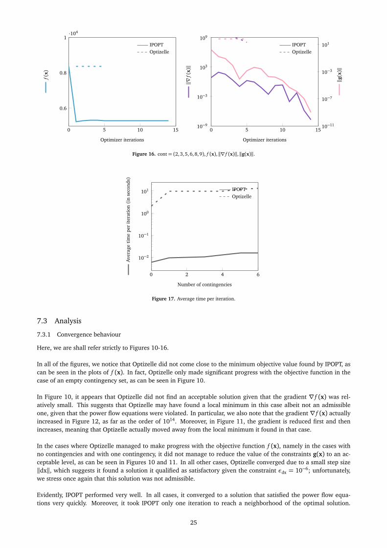
In Figures 10-16 below, f (x) denotes the objective function, and g(x) denotes the constraint functions, i.e., thepower flow equations. Each figure contains two plots corresponding to a contingency set with cardinality |G | = i,for i = 0, ..., 6. On the left plot, we plot f (x); on the right plot, we plot ∥∇ f (x)∥ and ∥g(x)∥; both plots are madeagainst the number of iterations. We note that there are two y-axes in the plots on the right-hand side of each figure,with the data corresponding to the colour of the y-axis labels. We represent the data from IPOPT with a continuousline, and the data from Optizelle with a loosely dashed line.

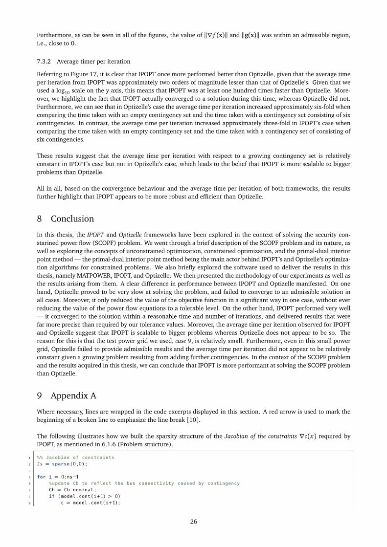
After these figures, we present the average time per iteration in Figure 17.

We will analyze Figures 10-17 after having presented them.

22

0 1,000 2,000 3,000 4,000 5,000

0.6

0.8

1·104

Optimizer iterations

f(x)

IPOPTOptizelle

0 20 40 60 80 10010−10

10−4

102

108


∥∇f(

x)∥

IPOPTOptizelle

10−11

10−7

10−3

101

∥g(x)∥

Figure 10. cont= no contingencies, f (x),∥∇ f (x)∥,∥g(x)∥.

0 20 40 60 80 100

0.6

0.8

1·104


f(x)

IPOPTOptizelle

0 500 1,000 1,500 2,00010−10

10−4

102

108


∥∇f(

x)∥

IPOPTOptizelle

10−11

10−7

10−3

101

∥g(x)∥

Figure 11. cont= 2, f (x),∥∇ f (x)∥,∥g(x)∥.

0 5 10 15

0.6

0.8

1·104


f(x)

IPOPTOptizelle

0 5 10 1510−10

10−2

106

1014


∥∇f(

x)∥

IPOPTOptizelle

10−11

10−7

10−3

101

∥g(x)∥

Figure 12. cont= (2, 3), f (x),∥∇ f (x)∥,∥g(x)∥.

23

0 5 10 15

0.6

0.8

1·104


f(x)

IPOPTOptizelle

0 5 10 1510−10

10−4

102

108


∥∇f(

x)∥

IPOPTOptizelle

10−11

10−7

10−3

101

∥g(x)∥

Figure 13. cont= (2, 3, 5), f (x),∥∇ f (x)∥,∥g(x)∥.

0 5 10 15

0.6

0.8

1·104


f(x)

IPOPTOptizelle

0 5 10 1510−10

10−4

102

108


∥∇f(

x)∥

IPOPTOptizelle

10−11

10−7

10−3

101

∥g(x)∥

Figure 14. cont= (2, 3, 5, 6), f (x),∥∇ f (x)∥,∥g(x)∥.

0 5 10 15

0.6

0.8

1·104


f(x)

IPOPTOptizelle

0 5 10 1510−13

10−6

101

108


∥∇f(

x)∥

IPOPTOptizelle

10−10

10−6

10−2

102

∥g(x)∥

Figure 15. cont= (2, 3, 5, 6, 8), f (x),∥∇ f (x)∥,∥g(x)∥.

24

0 5 10 15

0.6

0.8

1·104


f(x)

IPOPTOptizelle

0 5 10 1510−9

10−3

103

109


∥∇f(

x)∥

IPOPTOptizelle

10−11

10−7

10−3

101

∥g(x)∥

Figure 16. cont= (2, 3, 5, 6, 8, 9), f (x),∥∇ f (x)∥,∥g(x)∥.

0 2 4 6

10−2

10−1

100

101

Number of contingencies

Ave

rage

tim

epe

rit

erat

ion

(in

seco

nds)

IPOPTOptizelle

Figure 17. Average time per iteration.

7.3 Analysis

7.3.1 Convergence behaviour

Here, we are shall refer strictly to Figures 10-16.

In all of the figures, we notice that Optizelle did not come close to the minimum objective value found by IPOPT, ascan be seen in the plots of f (x). In fact, Optizelle only made significant progress with the objective function in thecase of an empty contingency set, as can be seen in Figure 10.

In Figure 10, it appears that Optizelle did not find an acceptable solution given that the gradient ∇ f (x) was rel-atively small. This suggests that Optizelle may have found a local minimum in this case albeit not an admissibleone, given that the power flow equations were violated. In particular, we also note that the gradient ∇ f (x) actuallyincreased in Figure 12, as far as the order of 1014. Moreover, in Figure 11, the gradient is reduced first and thenincreases, meaning that Optizelle actually moved away from the local minimum it found in that case.

In the cases where Optizelle managed to make progress with the objective function f (x), namely in the cases withno contingencies and with one contingency, it did not manage to reduce the value of the constraints g(x) to an ac-ceptable level, as can be seen in Figures 10 and 11. In all other cases, Optizelle converged due to a small step size∥dx∥, which suggests it found a solution it qualified as satisfactory given the constraint εdx = 10−6; unfortunately,we stress once again that this solution was not admissible.

Evidently, IPOPT performed very well. In all cases, it converged to a solution that satisfied the power flow equa-tions very quickly. Moreover, it took IPOPT only one iteration to reach a neighborhood of the optimal solution.

25

Furthermore, as can be seen in all of the figures, the value of ∥∇ f (x)∥ and ∥g(x)∥ was within an admissible region,i.e., close to 0.

7.3.2 Average timer per iteration

Referring to Figure 17, it is clear that IPOPT once more performed better than Optizelle, given that the average timeper iteration from IPOPT was approximately two orders of magnitude lesser than that of Optizelle’s. Given that weused a log10 scale on the y axis, this means that IPOPT was at least one hundred times faster than Optizelle. More-over, we highlight the fact that IPOPT actually converged to a solution during this time, whereas Optizelle did not.Furthermore, we can see that in Optizelle’s case the average time per iteration increased approximately six-fold whencomparing the time taken with an empty contingency set and the time taken with a contingency set consisting of sixcontingencies. In contrast, the average time per iteration increased approximately three-fold in IPOPT’s case whencomparing the time taken with an empty contingency set and the time taken with a contingency set of consisting ofsix contingencies.

These results suggest that the average time per iteration with respect to a growing contingency set is relativelyconstant in IPOPT’s case but not in Optizelle’s case, which leads to the belief that IPOPT is more scalable to biggerproblems than Optizelle.

All in all, based on the convergence behaviour and the average time per iteration of both frameworks, the resultsfurther highlight that IPOPT appears to be more robust and efficient than Optizelle.

8 Conclusion

In this thesis, the IPOPT and Optizelle frameworks have been explored in the context of solving the security con-starined power flow (SCOPF) problem. We went through a brief description of the SCOPF problem and its nature, aswell as exploring the concepts of unconstrained optimization, constrained optimization, and the primal-dual interiorpoint method — the primal-dual interior point method being the main actor behind IPOPT’s and Optizelle’s optimiza-tion algorithms for constrained problems. We also briefly explored the software used to deliver the results in thisthesis, namely MATPOWER, IPOPT, and Optizelle. We then presented the methodology of our experiments as well asthe results arising from them. A clear difference in performance between IPOPT and Optizelle manifested. On onehand, Optizelle proved to be very slow at solving the problem, and failed to converge to an admissible solution inall cases. Moreover, it only reduced the value of the objective function in a significant way in one case, without everreducing the value of the power flow equations to a tolerable level. On the other hand, IPOPT performed very well— it converged to the solution within a reasonable time and number of iterations, and delivered results that werefar more precise than required by our tolerance values. Moreover, the average time per iteration observed for IPOPTand Optizelle suggest that IPOPT is scalable to bigger problems whereas Optizelle does not appear to be so. Thereason for this is that the test power grid we used, case 9, is relatively small. Furthermore, even in this small powergrid, Optizelle failed to provide admissible results and the average time per iteration did not appear to be relativelyconstant given a growing problem resulting from adding further contingencies. In the context of the SCOPF problemand the results acquired in this thesis, we can conclude that IPOPT is more performant at solving the SCOPF problemthan Optizelle.

9 Appendix A

Where necessary, lines are wrapped in the code excerpts displayed in this section. A red arrow is used to mark thebeginning of a broken line to emphasize the line break [10].

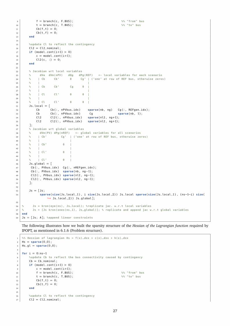
The following illustrates how we built the sparsity structure of the Jacobian of the constraints ∇c(x) required byIPOPT, as mentioned in 6.1.6 (Problem structure).

1 %% Jacobian of constraints

2 Js = sparse (0 ,0) ;3

4 for i = 0:ns−15 %update Cb to reflect the bus connectivity caused by contingency

6 Cb = Cb_nominal ;7 if (model . cont (i+1) > 0)8 c = model . cont (i+1) ;

26

9 f = branch (c , F_BUS ) ; %% "from" bus

10 t = branch (c , T_BUS ) ; %% "to" bus

11 Cb (f , t ) = 0;12 Cb (t , f ) = 0;13 end

14

15 %update Cl to reflect the contingency

16 Cl2 = Cl2_nominal ;17 if (model . cont (i+1) > 0)18 c = model . cont (i+1) ;19 Cl2 (c , : ) = 0;20 end

21

22 % Jacobian wrt local variables

23 % dVa dVm(nPV) dQg dPg(REF) <- local variables for each scenario

24 % | Cb Cb’ 0 Cg’ | (’one’ at row of REF bus, otherwise zeros)

25 % | |

26 % | Cb Cb’ Cg 0 |

27 % | |

28 % | Cl Cl’ 0 0 |

29 % | |

30 % | Cl Cl’ 0 0 |

31 Js_local = [32 Cb Cb ( : , nPVbus_idx ) sparse (nb , ng ) Cg ( : , REFgen_idx ) ;33 Cb Cb ( : , nPVbus_idx ) Cg sparse (nb , 1) ;34 Cl2 Cl2 ( : , nPVbus_idx ) sparse (nl2 , ng+1) ;35 Cl2 Cl2 ( : , nPVbus_idx ) sparse (nl2 , ng+1) ;36 ] ;37 % Jacobian wrt global variables

38 % dVm(PV) dPg(nREF) <- global variables for all scenarios

39 % | Cb’ Cg’ | (’one’ at row of REF bus, otherwise zeros)

40 % | |

41 % | Cb’ 0 |

42 % | |

43 % | Cl’ 0 |

44 % | |

45 % | Cl’ 0 |

46 Js_global = [47 Cb ( : , PVbus_idx ) Cg ( : , nREFgen_idx ) ;48 Cb ( : , PVbus_idx ) sparse (nb , ng−1) ;49 Cl2 ( : , PVbus_idx ) sparse (nl2 , ng−1) ;50 Cl2 ( : , PVbus_idx ) sparse (nl2 , ng−1) ;51 ] ;52

53 Js = [Js ;54 sparse (size (Js_local , 1 ) , i size (Js_local , 2 ) ) Js_local sparse (size (Js_local , 1 ) , (ns−1−i ) size (

,→ Js_local , 2 ) ) Js_global ] ;55

56 % Js = kron(eye(ns), Js_local); %replicate jac. w.r.t local variables

57 % Js = [Js kron(ones(ns,1), Js_global)]; % replicate and append jac w.r.t global variables

58 end

59 Js = [Js ; A ] ; %append linear constraints

The following illustrates how we built the sparsity structure of the Hessian of the Lagrangian function required byIPOPT, as mentioned in 6.1.6 (Problem structure).

1 %% Hessian of lagrangian Hs = f(x)_dxx + c(x)_dxx + h(x)_dxx

2 Hs = sparse (0 ,0) ;3 Hs_gl = sparse (0 ,0) ;4

5 for i = 0:ns−16 %update Cb to reflect the bus connectivity caused by contingency

7 Cb = Cb_nominal ;8 if (model . cont (i+1) > 0)9 c = model . cont (i+1) ;

10 f = branch (c , F_BUS ) ; %% "from" bus

11 t = branch (c , T_BUS ) ; %% "to" bus

12 Cb (f , t ) = 0;13 Cb (t , f ) = 0;14 end

15

16 %update Cl to reflect the contingency

17 Cl2 = Cl2_nominal ;

27

18 if (model . cont (i+1) > 0)19 c = model . cont (i+1) ;20 Cl2 (c , : ) = 0;21 end

22

23 %--- hessian wrt. scenario local variables ---

24

25 % dVa dVm(nPV) dQg dPg(REF)

26 % dVa | Cb Cb’ 0 0 |

27 % | |

28 % dVm(nPV)| Cb’ Cb’ 0 0 |

29 % | |

30 % dQg | 0 0 0 0 |

31 % | |

32 % dPg(REF)| 0 0 0 Cg’ | (only nominal case has Cg’, because it is used in cost

,→ function)

33

34 Hs_ll =[35 Cb Cb ( : , nPVbus_idx ) sparse (nb , ng+1) ; %assuming 1 REF gen

36 Cb (nPVbus_idx , : ) Cb (nPVbus_idx , nPVbus_idx ) sparse (length (nPVbus_idx ) , ng+1) ;37 sparse (ng+1, nb+length (nPVbus_idx )+ng+1) ;38 ] ;39 %replicate hess. w.r.t local variables

40 %Hs = kron(eye(ns), Hs_ll);

41

42 %set d2Pg(REF) to 1 in nominal case

43 if (i==0)44 Hs_ll (nb+length (nPVbus_idx )+ng+1, nb+length (nPVbus_idx )+ng+1) = 1;45 end

46

47 %--- hessian w.r.t local-global variables ---

48

49 % dVm(PV) dPg(nREF)

50 % dVa | Cb’ 0 |

51 % | |

52 % dVm(nPV)| Cb’ 0 |

53 % | |

54 % dQg | 0 0 |

55 % | |

56 % dPg(REF)| 0 0 |

57 Hs_lg = [58 Cb ( : , PVbus_idx ) sparse (nb , ng−1) ;59 Cb (nPVbus_idx , PVbus_idx ) sparse (length (nPVbus_idx ) , ng−1) ;60 sparse (ng+length (REFgen_idx ) , length (PVbus_idx )+ng−1)61 ] ;62 %Hs_lg = kron(ones(ns,1), Hs_lg);

63

64 Hs = [Hs ;65 sparse (size (Hs_ll , 1 ) , i size (Hs_ll , 2 ) ) Hs_ll sparse (size (Hs_ll , 1 ) , (ns−1−i ) size (Hs_ll , 2 ) )

,→ Hs_lg ] ;66 Hs_gl = [Hs_gl Hs_lg ’ ] ;67

68 end

69

70 % --- hessian w.r.t global variables ---

71

72 % dVm(PV) dPg(nREF)

73 % dVm(PV) | Cb’ 0 |

74 % | |

75 % dPg(nREF)| 0 f_xx’ |

76 Hs_gg =[77 Cb_nominal (PVbus_idx , PVbus_idx ) sparse (length (PVbus_idx ) , ng−1) ;78 sparse (ng−1, length (PVbus_idx ) ) eye (ng−1) ;79 ] ;80

81 % --- Put together local and global hessian ---

82 % local hessians sits at (1,1) block

83 % hessian w.r.t global variables is appended to lower right corner (2,2)

84 % and hessian w.r.t local/global variables to the (1,2) and (2,1) blocks

85 % (l) (g)

86 % (l) | Hs_ll Hs_lg |

87 % | |

88 % (g) | Hs_gl Hs_gg |

28

89 Hs = [Hs ;90 Hs_gl Hs_gg ] ;91

92

93 Hs = tril (Hs ) ;

The following displays the definition of the functions required by IPOPT, as mentioned in 6.1.7 (Evaluation of problemfunctions).

1 function f = objective (x , d )2 mpc = get_mpc (d . om ) ;3 ns = size (d . cont , 1) ; %% number of scenarios (nominal + ncont)

4

5 % use nominal case to evaluate cost fcn (only pg/qg are relevant)

6 idx_nom = d . index . getGlobalIndices (mpc , ns , 0) ;7 [VAscopf , VMscopf , PGscopf , QGscopf ] = d . index . getLocalIndicesSCOPF (mpc ) ;8

9 f = opf_costfcn (x (idx_nom ( [ VAscopf VMscopf PGscopf QGscopf ] ) ) , d . om ) ;

1 function grad = gradient (x , d )2 mpc = get_mpc (d . om ) ;3 ns = size (d . cont , 1) ; %% number of scenarios (nominal + ncont)

4

5 %evaluate grad of nominal case

6 idx_nom = d . index . getGlobalIndices (mpc , ns , 0) ;7 [VAscopf , VMscopf , PGscopf , QGscopf ] = d . index . getLocalIndicesSCOPF (mpc ) ;8 [VAopf , VMopf , PGopf , QGopf ] = d . index . getLocalIndicesOPF (mpc ) ;9

10 [f , df , d2f ] = opf_costfcn (x (idx_nom ( [ VAscopf VMscopf PGscopf QGscopf ] ) ) , d . om ) ;11

12 grad = zeros (size (x , 1 ) ,1) ;13 grad (idx_nom (PGscopf ) ) = df (PGopf ) ; %nonzero only nominal case Pg

1 function constr = constraints (x , d )2 mpc = get_mpc (d . om ) ;3 nb = size (mpc . bus , 1) ; %% number of buses

4 ng = size (mpc . gen , 1) ; %% number of gens

5 nl = size (mpc . branch , 1) ; %% number of branches

6 ns = size (d . cont , 1) ; %% number of scenarios (nominal + ncont)

7 NCONSTR = 2 nb + 2 nl ;8

9 constr = zeros (ns ( NCONSTR ) , 1) ;10

11 [VAscopf , VMscopf , PGscopf , QGscopf ] = d . index . getLocalIndicesSCOPF (mpc ) ;12 [VAopf , VMopf , PGopf , QGopf ] = d . index . getLocalIndicesOPF (mpc ) ;13

14 for i = 0:ns−115 cont = d . cont (i+1) ;16 idx = d . index . getGlobalIndices (mpc , ns , i ) ;17 [Ybus , Yf , Yt ] = makeYbus (mpc . baseMVA , mpc . bus , mpc . branch , cont ) ;18 [hn_local , gn_local ] = opf_consfcn (x (idx ( [ VAscopf VMscopf PGscopf QGscopf ] ) ) , d . om , Ybus , Yf , Yt , d .

,→ mpopt , d . il ) ;19 constr (i ( NCONSTR ) + (1 : NCONSTR ) ) = [ gn_local ; hn_local ] ;20 end

21

22 if ~isempty (d . A )23 constr = [constr ; d . A x ] ; %append linear constraints

24 end

1 function J = jacobian (x , d )2 mpc = get_mpc (d . om ) ;3 nb = size (mpc . bus , 1) ; %% number of buses



6 NCONSTR = 2 nb + 2 nl ; %% number of constraints (eq + ineq)

7

8 J = sparse (ns ( NCONSTR ) , size (x , 1 ) ) ;9

10 % get indices of REF gen and PV bus

11 [REFgen_idx , nREFgen_idx ] = d . index . getREFgens (mpc ) ;

29

12 [PVbus_idx , nPVbus_idx ] = d . index . getXbuses (mpc , 2 ) ; %2==PV13


17 for i = 0:ns−118 %compute local indices

19 idx = d . index . getGlobalIndices (mpc , ns , i ) ;20

21 cont = d . cont (i+1) ;22 [Ybus , Yf , Yt ] = makeYbus (mpc . baseMVA , mpc . bus , mpc . branch , cont ) ;23 [hn , gn , dhn , dgn ] = opf_consfcn (x (idx ( [ VAscopf VMscopf PGscopf QGscopf ] ) ) , d . om , Ybus , Yf , Yt , d .

,→ mpopt , d . il ) ;24 dgn = dgn ’ ;25 dhn = dhn ’ ;26

27 %jacobian wrt local variables

28 J (i NCONSTR + (1 : NCONSTR ) , idx ( [ VAscopf VMscopf (nPVbus_idx ) QGscopf PGscopf (REFgen_idx ) ] ) ) . . .29 = [dgn ( : , [ VAopf VMopf (nPVbus_idx ) QGopf PGopf (REFgen_idx ) ] ) ; . . .30 dhn ( : , [ VAopf VMopf (nPVbus_idx ) QGopf PGopf (REFgen_idx ) ] ) ] ;31 %jacobian wrt global variables

32 J (i NCONSTR + (1 : NCONSTR ) , idx ( [ VMscopf (PVbus_idx ) PGscopf (nREFgen_idx ) ] ) ) . . .33 = [dgn ( : , [VMopf (PVbus_idx ) PGopf (nREFgen_idx ) ] ) ; . . .34 dhn ( : , [VMopf (PVbus_idx ) PGopf (nREFgen_idx ) ] ) ] ;35 end

36 J = [J ; d . A ] ; %append Jacobian of linear constraints

1 function H = hessian (x , sigma , lambda , d )2 mpc = get_mpc (d . om ) ;3 nb = size (mpc . bus , 1) ; %% number of buses

4 ng = size (mpc . gen , 1) ; %% number of gens



7 NCONSTR = 2 nb + 2 nl ;8

9 H = sparse (size (x , 1 ) , size (x , 1 ) ) ;10


12 [REFgen_idx , nREFgen_idx ] = d . index . getREFgens (mpc ) ;13 [PVbus_idx , nPVbus_idx ] = d . index . getXbuses (mpc , 2 ) ; %2==PV14


18 for i = 0:ns−119 %compute local indices and its parts

20 idx = d . index . getGlobalIndices (mpc , ns , i ) ;21

22 cont = d . cont (i+1) ;23 [Ybus , Yf , Yt ] = makeYbus (mpc . baseMVA , mpc . bus , mpc . branch , cont ) ;24

25 lam . eqnonlin = lambda (i NCONSTR + ( 1 : 2 nb ) ) ;26 lam . ineqnonlin = lambda (i NCONSTR + 2 nb + ( 1 : 2 nl ) ) ;27 H_local = opf_hessfcn (x (idx ( [ VAscopf VMscopf PGscopf QGscopf ] ) ) , lam , sigma , d . om , Ybus , Yf , Yt , d

,→ . mpopt , d . il ) ;28

29 % H_ll (PG_ref relevant only in nominal case, added to global part)

30 H (idx ( [ VAscopf VMscopf (nPVbus_idx ) QGscopf ] ) , idx ( [ VAscopf VMscopf (nPVbus_idx ) QGscopf ] ) ) = . . .31 H_local ( [ VAopf VMopf (nPVbus_idx ) QGopf ] , [VAopf VMopf (nPVbus_idx ) QGopf ] ) ;32

33 % H_lg and H_gl (PG parts are implicitly zero, could leave them out)

34 H (idx ( [ VAscopf VMscopf (nPVbus_idx ) QGscopf PGscopf (REFgen_idx ) ] ) , idx ( [ VMscopf (PVbus_idx ) PGscopf (,→ nREFgen_idx ) ] ) ) = . . .

35 H_local ( [ VAopf VMopf (nPVbus_idx ) QGopf PGopf (REFgen_idx ) ] , [VMopf (PVbus_idx ) PGopf (,→ nREFgen_idx ) ] ) ;

36 H (idx ( [ VMscopf (PVbus_idx ) PGscopf (nREFgen_idx ) ] ) , idx ( [ VAscopf VMscopf (nPVbus_idx ) QGscopf PGscopf

,→ (REFgen_idx ) ] ) ) = . . .37 H_local ( [ VMopf (PVbus_idx ) PGopf (nREFgen_idx ) ] , [VAopf VMopf (nPVbus_idx ) QGopf PGopf (

,→ REFgen_idx ) ] ) ;38

39 % H_gg hessian w.r.t global variables (and PG_ref_0)

40 if i == 0

30

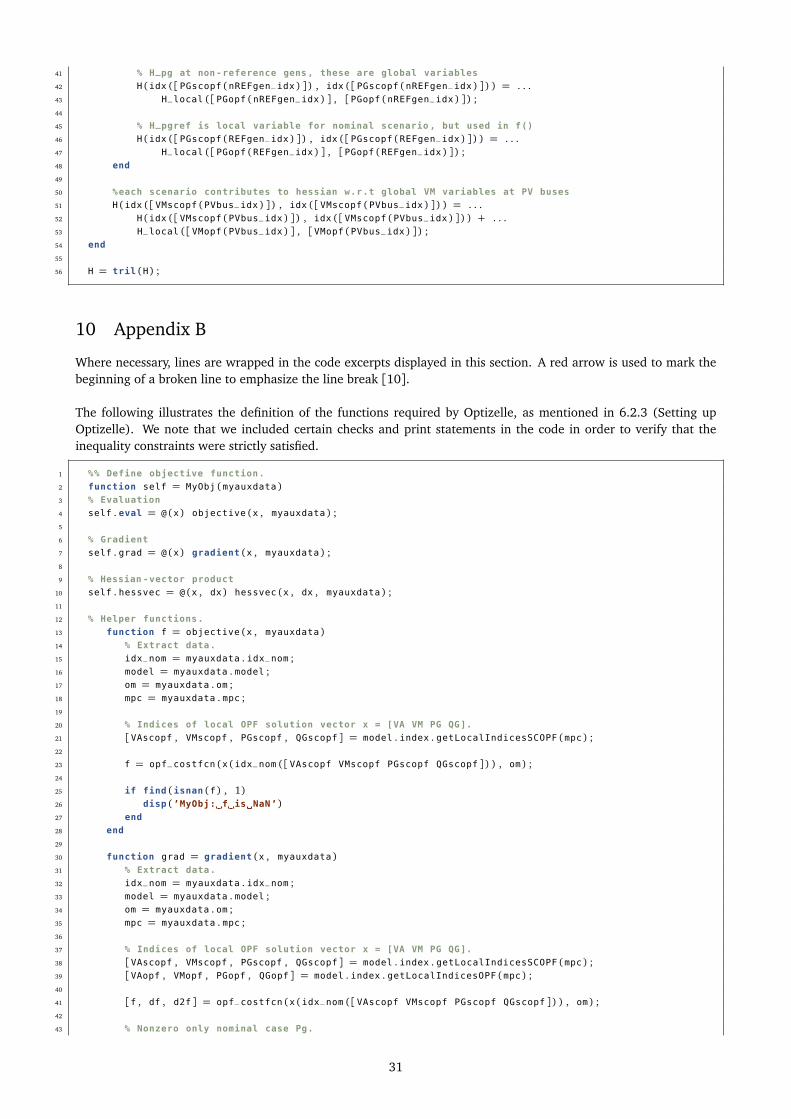
41 % H_pg at non-reference gens, these are global variables

42 H (idx ( [ PGscopf (nREFgen_idx ) ] ) , idx ( [ PGscopf (nREFgen_idx ) ] ) ) = . . .43 H_local ( [ PGopf (nREFgen_idx ) ] , [PGopf (nREFgen_idx ) ] ) ;44

45 % H_pgref is local variable for nominal scenario, but used in f()

46 H (idx ( [ PGscopf (REFgen_idx ) ] ) , idx ( [ PGscopf (REFgen_idx ) ] ) ) = . . .47 H_local ( [ PGopf (REFgen_idx ) ] , [PGopf (REFgen_idx ) ] ) ;48 end

49

50 %each scenario contributes to hessian w.r.t global VM variables at PV buses

51 H (idx ( [ VMscopf (PVbus_idx ) ] ) , idx ( [ VMscopf (PVbus_idx ) ] ) ) = . . .52 H (idx ( [ VMscopf (PVbus_idx ) ] ) , idx ( [ VMscopf (PVbus_idx ) ] ) ) + . . .53 H_local ( [ VMopf (PVbus_idx ) ] , [VMopf (PVbus_idx ) ] ) ;54 end

55

56 H = tril (H ) ;

10 Appendix B

Where necessary, lines are wrapped in the code excerpts displayed in this section. A red arrow is used to mark thebeginning of a broken line to emphasize the line break [10].

The following illustrates the definition of the functions required by Optizelle, as mentioned in 6.2.3 (Setting upOptizelle). We note that we included certain checks and print statements in the code in order to verify that theinequality constraints were strictly satisfied.

1 %% Define objective function.

2 function self = MyObj (myauxdata )3 % Evaluation

4 self . eval = @ (x ) objective (x , myauxdata ) ;5

6 % Gradient

7 self . grad = @ (x ) gradient (x , myauxdata ) ;8

9 % Hessian-vector product

10 self . hessvec = @ (x , dx ) hessvec (x , dx , myauxdata ) ;11

12 % Helper functions.

13 function f = objective (x , myauxdata )14 % Extract data.

15 idx_nom = myauxdata . idx_nom ;16 model = myauxdata . model ;17 om = myauxdata . om ;18 mpc = myauxdata . mpc ;19

20 % Indices of local OPF solution vector x = [VA VM PG QG].

21 [VAscopf , VMscopf , PGscopf , QGscopf ] = model . index . getLocalIndicesSCOPF (mpc ) ;22

23 f = opf_costfcn (x (idx_nom ( [ VAscopf VMscopf PGscopf QGscopf ] ) ) , om ) ;24

25 if find (isnan (f ) , 1)26 disp (’MyObj: f is NaN’)27 end

28 end

29

30 function grad = gradient (x , myauxdata )31 % Extract data.



38 [VAscopf , VMscopf , PGscopf , QGscopf ] = model . index . getLocalIndicesSCOPF (mpc ) ;39 [VAopf , VMopf , PGopf , QGopf ] = model . index . getLocalIndicesOPF (mpc ) ;40

41 [f , df , d2f ] = opf_costfcn (x (idx_nom ( [ VAscopf VMscopf PGscopf QGscopf ] ) ) , om ) ;42

43 % Nonzero only nominal case Pg.

31

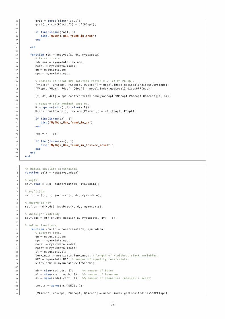
44 grad = zeros (size (x , 1 ) ,1) ;45 grad (idx_nom (PGscopf ) ) = df (PGopf ) ;46

47 if find (isnan (grad ) , 1)48 disp (’MyObj: NaN found in grad’)49 end

50

51 end

52

53 function res = hessvec (x , dx , myauxdata )54 % Extract data.




64 [f , df , d2f ] = opf_costfcn (x (idx_nom ( [ VAscopf VMscopf PGscopf QGscopf ] ) ) , om ) ;65

66 % Nonzero only nominal case Pg.

67 H = sparse (size (x , 1 ) , size (x , 1 ) ) ;68 H (idx_nom (PGscopf ) , idx_nom (PGscopf ) ) = d2f (PGopf , PGopf ) ;69

70 if find (isnan (dx ) , 1)71 disp (’MyObj: NaN found in dx’)72 end

73

74 res = H dx ;75

76 if find (isnan (res ) , 1)77 disp (’MyObj: NaN found in hessvec result’)78 end

79 end

80 end

1 %% Define equality constraints.

2 function self = MyEq (myauxdata )3

4 % y=g(x)


7 % y=g’(x)dx


10 % xhat=g’(x)*dy

11 self . ps = @ (x , dy ) jacobvec (x , dy , myauxdata ) ;12

13 % xhat=(g’’(x)dx)*dy

14 self . pps = @ (x , dx , dy ) hessian (x , myauxdata , dy ) dx ;15


17 function constr = constraints (x , myauxdata )18 % Extract data.

19 om = myauxdata . om ;20 mpc = myauxdata . mpc ;21 model = myauxdata . model ;22 mpopt = myauxdata . mpopt ;23 il = myauxdata . il ;24 lenx_no_s = myauxdata . lenx_no_s ; % length of x without slack variables.

25 NEQ = myauxdata . NEQ ; % number of equality constraints.

26 withSlacks = myauxdata . withSlacks ;27

28 nb = size (mpc . bus , 1) ; %% number of buses


30 ns = size (model . cont , 1) ; %% number of scenarios (nominal + ncont)

31

32 constr = zeros (ns ( NEQ ) , 1) ;33

34 [VAscopf , VMscopf , PGscopf , QGscopf ] = model . index . getLocalIndicesSCOPF (mpc ) ;

32

35

36 for i = 0:ns−137 cont = model . cont (i+1) ;38 idx = model . index . getGlobalIndices (mpc , ns , i ) ;39

40 [Ybus , Yf , Yt ] = makeYbus (mpc . baseMVA , mpc . bus , mpc . branch , cont ) ;41 [hn_local , gn_local ] = opf_consfcn (x (idx ( [ VAscopf VMscopf PGscopf QGscopf ] ) ) , om , Ybus , Yf ,

,→ Yt , mpopt , il ) ;42

43 if withSlacks

44 % Extract slack variable(s) s from x.

45 % s = [s0, s1, ... , sNS]

46 s = x (lenx_no_s + i 2 nl + ( 1 : 2 nl ) ) ;47

48 % Since h(x) <= 0 in Matpower, -h(x) - s = 0, s >= 0

49 % as required by Optizelle.

50 constr (i ( NEQ ) + (1 : NEQ ) ) = [ gn_local ; −hn_local − s ] ;51 else

52 constr (i ( NEQ ) + (1 : NEQ ) ) = gn_local ;53 end

54 end

55

56

57 %% Test for Inf, -Inf, and NaN in constr.

58 if find (constr == Inf , 1)59 disp (’MyEq: Inf found in constr’)60 end

61

62 if find (constr == −Inf , 1)63 disp (’MyEq: -Inf found in constr’)64 end

65

66 if find (isnan (constr ) , 1)67 disp (’MyEq: NaN found in constr’)68 end

69 end

70

71 function jvec = jacobvec (x , d , myauxdata )72 % Extract data.

73 om = myauxdata . om ;74 mpc = myauxdata . mpc ;75 model = myauxdata . model ;76 mpopt = myauxdata . mpopt ;77 il = myauxdata . il ;78 lenx_no_s = myauxdata . lenx_no_s ; % length of x without slack variables.

79 NEQ = myauxdata . NEQ ; % number of equality constraints.

80 withSlacks = myauxdata . withSlacks ;81

82




86


88 [REFgen_idx , nREFgen_idx ] = model . index . getREFgens (mpc ) ;89 [PVbus_idx , nPVbus_idx ] = model . index . getXbuses (mpc , 2 ) ; %2==PV90


94 % -Id. Placed in the lower-right "corner" of each scenario’s

95 % Jacobian matrix.

96 neg_identity = −sparse (eye ( 2 nl , 2 nl ) ) ;97

98 J = sparse (ns NEQ , length (x ) ) ;99

100 for i = 0:ns−1101 idx = model . index . getGlobalIndices (mpc , ns , i ) ;102

103 cont = model . cont (i+1) ;104 [Ybus , Yf , Yt ] = makeYbus (mpc . baseMVA , mpc . bus , mpc . branch , cont ) ;105 [hn , gn , dhn , dgn ] = opf_consfcn (x (idx ( [ VAscopf VMscopf PGscopf QGscopf ] ) ) , om , Ybus , Yf , Yt ,

,→ mpopt , il ) ;

33

106

107 % Transpose since opf_consfcn transposed solutions.

108 % Take negative since Matpower requires h(x) <= 0 but

109 % Optizelle requires h(x) >= 0.

110 dhn = −dhn ’ ;111 dgn = dgn ’ ;112

113 if withSlacks


115 J (i NEQ + (1 : NEQ ) , idx ( [ VAscopf VMscopf (nPVbus_idx ) QGscopf PGscopf (REFgen_idx ) ] ) ) = [dgn,→ ( : , [ VAopf VMopf (nPVbus_idx ) QGopf PGopf (REFgen_idx ) ] ) ; . . .

116 dhn ( : , [ VAopf VMopf (nPVbus_idx ) QGopf PGopf (REFgen_idx ) ] ) ] ;117 %jacobian wrt global variables

118 J (i NEQ + (1 : NEQ ) , idx ( [ VMscopf (PVbus_idx ) PGscopf (nREFgen_idx ) ] ) ) = [dgn ( : , [VMopf (,→ PVbus_idx ) PGopf (nREFgen_idx ) ] ) ; . . .

119 dhn ( : , [VMopf (PVbus_idx ) PGopf (nREFgen_idx ) ] ) ] ;120

121 else


123 J (i NEQ + (1 : NEQ ) , idx ( [ VAscopf VMscopf (nPVbus_idx ) QGscopf PGscopf (REFgen_idx ) ] ) ) = dgn

,→ ( : , [ VAopf VMopf (nPVbus_idx ) QGopf PGopf (REFgen_idx ) ] ) ;124

125 %jacobian wrt global variables

126 J (i NEQ + (1 : NEQ ) , idx ( [ VMscopf (PVbus_idx ) PGscopf (nREFgen_idx ) ] ) ) = dgn ( : , [VMopf (,→ PVbus_idx ) PGopf (nREFgen_idx ) ] ) ;

127 end

128

129 % Set corner of Jacobian of this scenario to -Id.

130 % Number of rows in dgn is 2*nb; in dhn it is 2*nl.

131 % Number of columns in dgn, and dhn, is lenx_no_s.

132 % Structure of Jacobian in scenario i is:

133 % J = [dgn, 0; dhn, -Id]. Hence why we use following row and

134 % column indices.

135 % Note: -Id has dimensions 2*nl by 2*nl.

136 %

137 % Considering the system of slack variables, we have

138 % [g(x); h(x) - s] for the equality constraints.

139 % As we can see, we have 0s in the upper right corner of J since the

140 % partial derivative of the constraints g(x) w.r.t. the slack variables

141 % is 0, since g(x) does not at all depend on s.

142 % Similarly, we have -Id in the specified (lower-right) corner

143 % given the constraints w.r.t. the slack variables are

144 % h(x) - s: taking the partial derivative of h(x) - s w.r.t. the slack

145 % variables yields the -Id matrix.

146 if withSlacks

147 J (i NEQ + 2 nb + ( 1 : 2 nl ) , lenx_no_s + i 2 nl + ( 1 : 2 nl ) ) = neg_identity ;148 end

149 end

150

151 dType = 0;152 if (size (d , 1) == size (x , 1) ) % case: d == dx

153 dType = ’dx’ ;154 jvec = J d ;155 elseif (size (d , 1) == ns NEQ ) % case: d == dy

156 jvec = J ’ d ;157 dType = ’dy’ ;158 end

159

160 %% Test for Inf, -Inf, and NaN in d.

161 if find (d == Inf )162 fprintf (’MyEq: Inf found in %s\n’ , dType ) ;163 end

164

165 if find (d == −Inf )166 fprintf (’MyEq: -Inf found in %s\n’ , dType ) ;167 end

168

169 if find (isnan (d ) )170 fprintf (’MyEq: NaN found in %s\n’ , dType ) ;171 end

172

173 %% Test for Inf, -Inf, and NaN in jvec.

174 if find (jvec == Inf , 1)

34

175 disp (’MyEq: Inf found in jvec’)176 end

177

178 if find (jvec == −Inf , 1)179 disp (’MyEq: -Inf found in jvec’)180 end

181

182 if find (isnan (jvec ) , 1)183 disp (’MyEq: NaN found in jvec’)184 end

185 end

186

187 function H = hessian (x , myauxdata , dy )188 % Extract data.

189 il = myauxdata . il ;190 om = myauxdata . om ;191 mpc = myauxdata . mpc ;192 model = myauxdata . model ;193 mpopt = myauxdata . mpopt ;194 NEQ = myauxdata . NEQ ; % number of equality constraints.

195 NINEQ = myauxdata . NINEQ ;196 withSlacks = myauxdata . withSlacks ;197




201

202 H = sparse (size (x , 1 ) , size (x , 1 ) ) ;203


205 [REFgen_idx , nREFgen_idx ] = model . index . getREFgens (mpc ) ;206 [PVbus_idx , nPVbus_idx ] = model . index . getXbuses (mpc , 2 ) ; %2==PV207


211 sigma = 0;212

213 for i = 0:ns−1214 %compute local indices and its parts

215 idx = model . index . getGlobalIndices (mpc , ns , i ) ;216

217 cont = model . cont (i+1) ;218 [Ybus , Yf , Yt ] = makeYbus (mpc . baseMVA , mpc . bus , mpc . branch , cont ) ;219

220 % c(x) = [gn0; hn0 - s0; gn1; hn1 - s1; ... ; gnNs; hnNs - sNs]

221 % (Ns is the number of scenarios)

222 % where gn corresponds to equality constraints, hn corresponds to

223 % inequality constraints.

224 %

225 % The lagrange multipliers in the dy will be composed accordingly:

226 % dy = [lamEq0; lamIneq0; lamEq1; lamIneq1; ... ; lamEqNs; lamIneqNs]

227 % Hence why we need to extract the lagrange multipliers as

228 % follows.

229 lam . eqnonlin = dy (i NEQ + ( 1 : 2 nb ) , 1) ;230

231 if withSlacks

232 lam . ineqnonlin = dy (i NEQ + 2 nb + ( 1 : 2 nl ) , 1) ;233 else

234 lam . ineqnonlin = zeros (NINEQ , 1) ;235 end

236

237 % Take negative since Matpower requires h(x) <= 0 but

238 % Optizelle requires h(x) >= 0.

239 lam . ineqnonlin = −lam . ineqnonlin ;240

241 H_local = opf_hessfcn (x (idx ( [ VAscopf VMscopf PGscopf QGscopf ] ) ) , lam , sigma , om , Ybus , Yf , Yt

,→ , mpopt , il ) ;242

243 % H_ll (PG_ref relevant only in nominal case, added to global part)

244 H (idx ( [ VAscopf VMscopf (nPVbus_idx ) QGscopf ] ) , idx ( [ VAscopf VMscopf (nPVbus_idx ) QGscopf ] ) ),→ = . . .

245 H_local ( [ VAopf VMopf (nPVbus_idx ) QGopf ] , [VAopf VMopf (nPVbus_idx ) QGopf ] ) ;

35

246

247 % H_lg and H_gl (PG parts are implicitly zero, could leave them out)

248 H (idx ( [ VAscopf VMscopf (nPVbus_idx ) QGscopf PGscopf (REFgen_idx ) ] ) , idx ( [ VMscopf (PVbus_idx ),→ PGscopf (nREFgen_idx ) ] ) ) = . . .

249 H_local ( [ VAopf VMopf (nPVbus_idx ) QGopf PGopf (REFgen_idx ) ] , [VMopf (PVbus_idx ) PGopf (,→ nREFgen_idx ) ] ) ;

250 H (idx ( [ VMscopf (PVbus_idx ) PGscopf (nREFgen_idx ) ] ) , idx ( [ VAscopf VMscopf (nPVbus_idx ) QGscopf

,→ PGscopf (REFgen_idx ) ] ) ) = . . .251 H_local ( [ VMopf (PVbus_idx ) PGopf (nREFgen_idx ) ] , [VAopf VMopf (nPVbus_idx ) QGopf PGopf (

,→ REFgen_idx ) ] ) ;252

253 % H_gg hessian w.r.t global variables (and PG_ref_0)

254 if i == 0255 % H_pg at non-reference gens, these are global variables

256 H (idx ( [ PGscopf (nREFgen_idx ) ] ) , idx ( [ PGscopf (nREFgen_idx ) ] ) ) = . . .257 H_local ( [ PGopf (nREFgen_idx ) ] , [PGopf (nREFgen_idx ) ] ) ;258

259 % H_pgref is local variable for nominal scenario, but used in f()

260 H (idx ( [ PGscopf (REFgen_idx ) ] ) , idx ( [ PGscopf (REFgen_idx ) ] ) ) = . . .261 H_local ( [ PGopf (REFgen_idx ) ] , [PGopf (REFgen_idx ) ] ) ;262 end

263

264 %each scenario contributes to hessian w.r.t global VM variables at PV buses

265 H (idx ( [ VMscopf (PVbus_idx ) ] ) , idx ( [ VMscopf (PVbus_idx ) ] ) ) = . . .266 H (idx ( [ VMscopf (PVbus_idx ) ] ) , idx ( [ VMscopf (PVbus_idx ) ] ) ) + . . .267 H_local ( [ VMopf (PVbus_idx ) ] , [VMopf (PVbus_idx ) ] ) ;268 end

269

270 %% Test for Inf, -Inf, and NaN in H.

271 if find (H == Inf , 1)272 disp (’MyEq: Inf found in H’)273 end

274

275 if find (H == −Inf , 1)276 disp (’MyEq: -Inf found in H’)277 end

278

279 if find (isnan (H ) , 1)280 disp (’MyEq: NaN found in H’)281 end

282 end

283 end

1 %% Define inequality constraints.

2 function self = MyIneq (myauxdata )3 % z=h(x)


6 % z=h’(x)dx


9 % xhat=h’(x)*dz

10 self . ps = @ (x , dz ) jacobvec (x , dz , myauxdata ) ;11

12 % xhat=(h’’(x)dx)*dz

13 self . pps = @ (x , dx , dz ) sparse (length (x ) , length (x ) ) ;14


16 function constr = constraints (x , myauxdata )17 % Append constraints for xmin <= x <= xmax.

18 xmin = myauxdata . xmin ;19 xmax = myauxdata . xmax ;20

21 constr = [x − xmin ;22 xmax − x (1 : myauxdata . lenx_no_s ) ] ;23

24 %% Test for Inf, -Inf, and NaN in constr.

25 if find (constr == Inf , 1)26 disp (’MyIneq: Inf found in constr’)27 end

28

29 if find (constr == −Inf , 1)

36

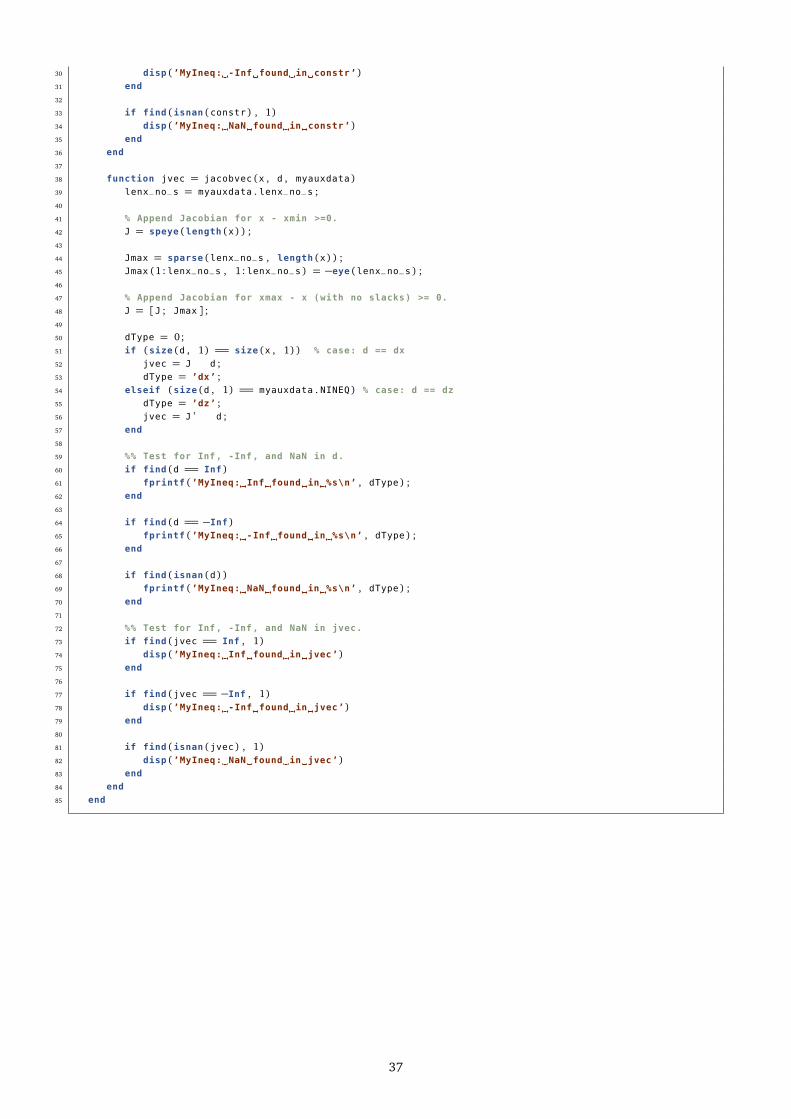
30 disp (’MyIneq: -Inf found in constr’)31 end

32

33 if find (isnan (constr ) , 1)34 disp (’MyIneq: NaN found in constr’)35 end

36 end

37

38 function jvec = jacobvec (x , d , myauxdata )39 lenx_no_s = myauxdata . lenx_no_s ;40

41 % Append Jacobian for x - xmin >=0.

42 J = speye (length (x ) ) ;43

44 Jmax = sparse (lenx_no_s , length (x ) ) ;45 Jmax (1 : lenx_no_s , 1: lenx_no_s ) = −eye (lenx_no_s ) ;46

47 % Append Jacobian for xmax - x (with no slacks) >= 0.

48 J = [J ; Jmax ] ;49

50 dType = 0;51 if (size (d , 1) == size (x , 1) ) % case: d == dx

52 jvec = J d ;53 dType = ’dx’ ;54 elseif (size (d , 1) == myauxdata . NINEQ ) % case: d == dz

55 dType = ’dz’ ;56 jvec = J ’ d ;57 end

58

59 %% Test for Inf, -Inf, and NaN in d.

60 if find (d == Inf )61 fprintf (’MyIneq: Inf found in %s\n’ , dType ) ;62 end

63

64 if find (d == −Inf )65 fprintf (’MyIneq: -Inf found in %s\n’ , dType ) ;66 end

67

68 if find (isnan (d ) )69 fprintf (’MyIneq: NaN found in %s\n’ , dType ) ;70 end

71

72 %% Test for Inf, -Inf, and NaN in jvec.

73 if find (jvec == Inf , 1)74 disp (’MyIneq: Inf found in jvec’)75 end

76

77 if find (jvec == −Inf , 1)78 disp (’MyIneq: -Inf found in jvec’)79 end

80

81 if find (isnan (jvec ) , 1)82 disp (’MyIneq: NaN found in jvec’)83 end

84 end

85 end

37

References

[1] J. Asprion. The matlab interface for ipopt. https://www.ethz.ch/content/dam/ethz/

special-interest/mavt/dynamic-systems-n-control/idsc-dam/Research_Onder/Downloads/IPOPT/

IPOPT_MatlabInterface_V0p1.pdf, 2013.

[2] COIN-OR. Ipopt frequently asked questions. https://projects.coin-or.org/Ipopt/wiki/FAQ, 2010.

[3] R. D. Zimmerman, C. E. Murillo-Sánchez, and R. J. Thomas. Matpower: Steadystate operations, planning andanalysis tools for power systems research and education. Power Systems, IEEE Transactions on, 26(1):12–19,February 2011. http://ieeexplore.ieee.org/document/5491276/.

[4] C.-O. Foundation. Coin-or. https://www.coin-or.org/, 2016.

[5] Gjacquenot. Solution of example lp in karmarkar’s algorithm. blue lines show the constraints, red shows eachiteration of the algorithm. https://commons.wikimedia.org/wiki/File:Karmarkar.svg, 2015.

[6] D. Heeger. Linear systems theory. http://www.cns.nyu.edu/~david/handouts/linear-systems/

linear-systems.html, 2003.

[7] U. M. Ascher and C. Greif. A First Course in Numerical Methods. Society for Industrial and Applied MathematicsPhiladelphia, 2011. Chapter 9. Section 2: Unconstrained optimization.

[8] U. M. Ascher and C. Greif. A First Course in Numerical Methods. Society for Industrial and Applied MathematicsPhiladelphia, 2011. Chapter 9. Section 3: Constrained optimization.

[9] MathWorks. Matlab. https://ch.mathworks.com/products/matlab.html, 2017.

[10] H. Menke. lstlisting line wrapping. https://tex.stackexchange.com/questions/116534/

lstlisting-line-wrapping, 2013.

[11] A. Optimization inc. and B. Web Design. Ampl. http://ampl.com/, 2013.

[12] D. Orban. Cuter. http://www.cuter.rl.ac.uk//, 2011.

[13] D. P. Bertsekas. Nonlinear Programming. Athena Scientific, 2 edition, 1999.

[14] A. Wächter and L. T. Biegler. On the implementation of a primal-dual interior point filter line search algorithmfor large-scale nonlinear programming. https://projects.coin-or.org/Ipopt, 2006.

[15] A. Wächter and L. T. Biegler. On the implementation of a primal-dual interior point filter line search algorithmfor large-scale nonlinear programming. Mathematical Programming, 106(1):25–57, 2006.

[16] J. Young. Optizelle. http://www.optimojoe.com/products/optizelle/, 2016.

[17] J. Young. Optizelle v1.2.0. Optimojoe, October 2016. http://www.optimojoe.com/uploads/reports/Optizelle-1.2.0-a4.pdf.

[18] J. Young. Infeasible initial guess. http://forum.optimojoe.com/t/infeasible-initial-guess/46, 2017.

38

https://www.ethz.ch/content/dam/ethz/special-interest/mavt/dynamic-systems-n-control/idsc-dam/Research_Onder/Downloads/IPOPT/IPOPT_MatlabInterface_V0p1.pdf



https://projects.coin-or.org/Ipopt/wiki/FAQ

http://ieeexplore.ieee.org/document/5491276/

https://www.coin-or.org/

https://commons.wikimedia.org/wiki/File:Karmarkar.svg

http://www.cns.nyu.edu/~david/handouts/linear-systems/linear-systems.html

http://www.cns.nyu.edu/~david/handouts/linear-systems/linear-systems.html

https://ch.mathworks.com/products/matlab.html

https://tex.stackexchange.com/questions/116534/lstlisting-line-wrapping

https://tex.stackexchange.com/questions/116534/lstlisting-line-wrapping

http://ampl.com/

http://www.cuter.rl.ac.uk//

https://projects.coin-or.org/Ipopt

http://www.optimojoe.com/products/optizelle/

http://forum.optimojoe.com/t/infeasible-initial-guess/46

security constrained optimal power ﬂow problems

Documents