Abstract A coupled 1D physical-biological

model of Crater Lake is presented. The model

simulates the seasonal evolution of two functional

phytoplankton groups, total chlorophyll, and zoo-

plankton in good quantitative agreement with

observations from a 10-year monitoring study.

During the stratified period in summer and early

fall the model displays a marked vertical structure:

the phytoplankton biomass of the functional group

1, which represents diatoms and dinoflagellates,

has its highest concentration in the upper 40 m; the

phytoplankton biomass of group 2, which repre-

sents chlorophyta, chrysophyta, cryptomonads and

cyanobacteria, has its highest concentrations be-

tween 50 and 80 m, and phytoplankton chlorophyll

has its maximum at 120 m depth. A similar vertical

structure is a reoccurring feature in the available

data. In the model the key process allowing a

vertical separation between biomass and chloro-

phyll is photoacclimation. Vertical light attenua-

tion (i.e., water clarity) and the physiological

ability of phytoplankton to increase their cellular

chlorophyll-to-biomass ratio are ultimately deter-

mining the location of the chlorophyll maximum.

The location of the particle maxima on the other

hand is determined by the balance between growth

and losses and occurs where growth and losses

equal.The vertical particle flux simulated by our

model agrees well with flux measurements from a

sediment trap. This motivated us to revisit a pre-

viously published study by Dymond et al. (1996).

Dymond et al. used a box model to estimate the

vertical particle flux and found a discrepancy by a

factor 2.5–10 between their model-derived flux and

measured fluxes from a sediment trap. Their box

model neglected the exchange flux of dissolved

and suspended organic matter, which, as our model

and available data suggests is significant for the

Guest Editors: Gary L. Larson, Robert Collier, and MarkW. BuktenicaLong-term Limnological Research and Monitoring atCrater Lake, Oregon

K. Fennel (&)Institute of Marine and Coastal Sciences andDepartment of Geological Science, RutgersUniversity, New Brunswick 08901, New Jersey, USAe-mail: kfennel@marine.rutgers.edu

R. CollierCollege of Oceanic and Atmospheric Sciences,Oregon State University, Corvallis 97331, Oregon,USA

G. LarsonUSGS Forest and Rangeland Ecosystems Center,Forest Science Laboratory Oregon State University,Corvallis 97331, Oregon, USA

G. CrawfordDepartment of Oceanography, Humboldt StateUniversity, Arcata 95521, California, USA

E. BossSchool of Marine Sciences, University of Maine,Orono 04473, Maine, USA

Hydrobiologia (2007) 574:265–280

DOI 10.1007/s10750-006-2615-5

123

CRATER LAKE, OREGON

Seasonal nutrient and plankton dynamicsin a physical-biological model of Crater Lake

Katja Fennel Æ Robert Collier Æ Gary Larson ÆGreg Crawford Æ Emmanuel Boss

� Springer Science+Business Media B.V. 2007

vertical exchange of nitrogen. Adjustment of Dy-

mond et al.’s assumptions to account for dissolved

and suspended nitrogen yields a flux estimate that

is consistent with sediment trap measurements and

our model.

Keywords Physical-biological model Æ Deep

chlorophyll maximum Æ Photoacclimation ÆCrater Lake

Introduction

Crater Lake is an ultra-oligotrophic, isolated cal-

dera lake in the Cascade Mountains, Oregon.

With a maximum depth of 590 m it is the deepest

lake in the US and one of the clearest bodies of

water on Earth. Crater Lake is surrounded by

steep caldera walls, has a very small watershed

and only small inputs of allochthonous matter.

Most of the water entering the lake is direct pre-

cipitation onto its surface, which makes up 78% of

its watershed. The remainder enters as run off

from the caldera walls and as hydrothermal influx

from the bottom (Collier et al. 1991). Despite its

great depth, Crater Lake is relatively well-mixed.

The upper portion of the lake (upper 200 m) is

homogenized twice a year in early winter and late

spring by free convection and wind-mixing

(McManus et al. 1993). Partial ventilation of the

deep lake occurs during these mixing periods

when the upper water column is nearly isothermal

(McManus et al., 1993) and during sporadic deep-

mixing events (Crawford & Collier, 1997). Inde-

pendent estimates of the lake ventilation time

agree that the lake is ventilated on timescales of 1

to 5 years (Simpson, 1970; McManus et al., 1993;

Crawford & Collier, 1997). Depletion of inorganic

nitrogen species in the upper 200 m of the lake in

summer implies nitrogen-limitation of phyto-

plankton growth, although bioassays suggest

co-limitation by trace metals (Lane & Goldmann,

1984). Concentrations of inorganic phosphorus

and silicic acid are relatively high and nearly uni-

form throughout the water column (Larson et al.,

1996a). Vertical mixing is the most important

source of new nutrients for primary production in

the euphotic zone (Dymond et al., 1996).

Comparisons of upward nutrient fluxes based on

box-model considerations and measurements of

vertical particle fluxes from sediment traps reveal

large discrepancies, i.e. the particle flux falls short

of balancing the estimated upwelled nitrogen

(Dymond et al., 1996).

The populations of microorganisms show dis-

tinct vertical maxima during stratified conditions

(McIntire et al., 1996; Larson et al., 1996b;

Urbach et al., 2001). In July and August, diatoms

and dinoflagellates reach their maximum biomass

in the upper 20 m of the water column, isolated

from below by a pronounced thermocline. Chlo-

rophyta, chrysophyta and cryptophyta dominate

below the thermocline with biomass maxima

between 80 and 100 m (Fig. 1) coincident with

the vertical maximum of primary production

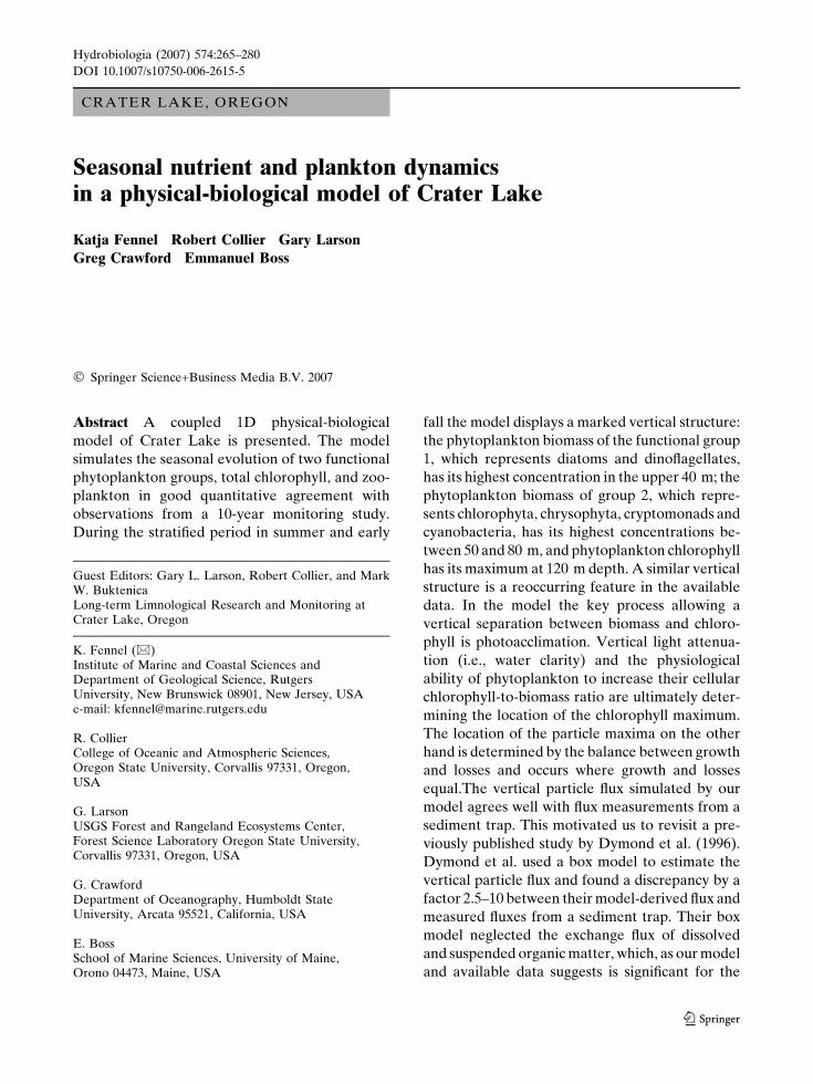
(McIntire et al., 1996). The chlorophyll concen-

tration has a deep maximum at a depth of 120 m,

separated from the phytoplankton biomass max-

imum by about 50 m (Fig. 2). The vertical sepa-

ration of the maxima in phytoplankton biomass

(in units of carbon or nitrogen) and chlorophyll is

mainly due to photoacclimation (Fennel & Boss,

2003) which results in dramatic vertical changes in

the chlorophyll to biomass ratio (Fig. 2) and im-

plies that the chlorophyll concentration does not

represent phytoplankton biomass.

We developed a coupled physical-biological

model of Crater Lake that captures the processes

thought to determine nutrient cycling and phy-

toplankton production at first-order in a simpli-

fied description of the food-web. We consider the

simplicity as valuable since it allows us to keep

the number of poorly known model parameters at

a minimum, but can elucidate dependencies and

regulating mechanisms not easily seen in the

observations alone. The model allows us to test

hypotheses about the factors determining spatial

and temporal patterns in species distribution,

chlorophyll concentration, and primary produc-

tion in relation to physical circulation processes.

Here we present results of a 1-year model simu-

lation in comparison with measurements obtained

during a 10-year monitoring study (Larson, this

issue), integrating the available data in a biomass-

based framework. We discuss factors leading to

the observed vertical distribution of phytoplank-

ton populations and compare model-simulated

vertical fluxes with particle flux measurements

266 Hydrobiologia (2007) 574:265–280

123

and box-model estimates (Dymond et al., 1996)

reconciling a previously reported mismatch.

Materials & methods

The biological model

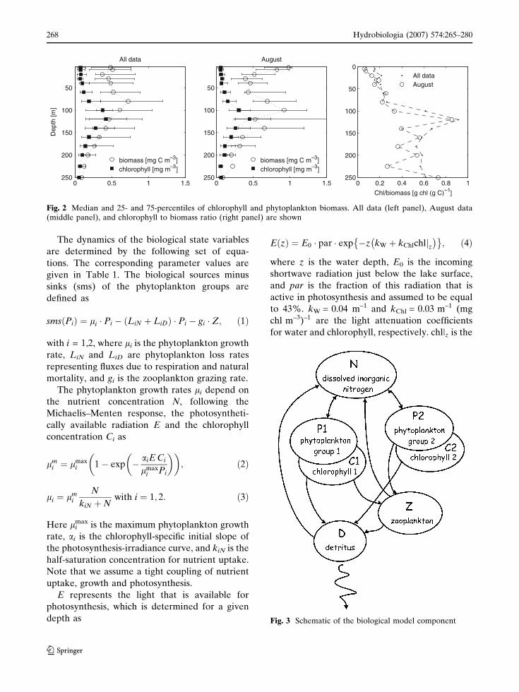
We formulated a relatively simple biological

model containing the following 7 state variables:

dissolved nitrogen N, two phytoplankton groups

P1 and P2, one group of zooplankton Z, one

detrital pool D, and the chlorophyll concentrations

C1 and C2 of P1 and P2, respectively (Fig. 3). All

variables are expressed in units of mmol N m–3

except the chlorophyll variables, which are

in mg chl m–3. Nitrogen was chosen as the nutri-

ent currency since Crater Lake is considered

nitrogen-limited (Lane & Goldman, 1984; Larsen

et al., 1996a). Note that the nutrient variable N

also includes dissolved organic nitrogen in addi-

tion to inorganic nitrogen. Technically detritus

includes both, particulate and dissolved pools of

organic nitrogen. However, the detritus variable

D in our model is subject to vertical sinking.

Hence, the dissolved organic nitrogen is more

realistically treated as part of the nutrient pool N.

The phytoplankton group P1 represents diatoms

and dinoflagellates, i.e. the phytoplankton domi-

nating in the upper 20 m of the water column. P2

comprises the remaining phytoplankton divisions

(chlorophyta, chrysophyta, cryptomonads and

cyanobacteria). The chlorophyll concentrations

C1 and C2 of P1 and P2 are included as dynamical

variables, to allow an explicit inclusion of photo-

acclimation.

50

100

150

200

2500 0.5 1 1.5

Phytoplankton group 1 (mmol N m–3)

Dep

th (

m)

August

50

100

150

200

2500 1 2 3 4

Phytoplankton group 2 (mmol N m –3)

50

100

150

200

2500 0.1 0.2 0.3 0.4 0.5

Zooplankton (mmol N m –3)

50

100

150

200

2500 0.5 1 1.5

Chlorophyll (mg m –3)

Fig. 1 Available August data from 1989 to 2001 (graybullets) and median with 25- and 75-percentiles (blackbullets). Diatoms and dinoflagellates comprise phyto-

plankton group 1. Chlorophyta, chrysophyta, cryptomo-nads and cyanobacteria comprise phytoplankton group 2

Hydrobiologia (2007) 574:265–280 267

123

The dynamics of the biological state variables

are determined by the following set of equa-

tions. The corresponding parameter values are

given in Table 1. The biological sources minus

sinks (sms) of the phytoplankton groups are

defined as

sms Pið Þ ¼ li � Pi � LiN þ LiDð Þ � Pi � gi � Z; ð1Þ

with i = 1,2, where li is the phytoplankton growth

rate, LiN and LiD are phytoplankton loss rates

representing fluxes due to respiration and natural

mortality, and gi is the zooplankton grazing rate.

The phytoplankton growth rates li depend on

the nutrient concentration N, following the

Michaelis–Menten response, the photosyntheti-

cally available radiation E and the chlorophyll

concentration Ci as

lmi ¼ lmax

i 1� exp � aiE Ci

lmaxi Pi

� �� �; ð2Þ

li ¼ lmi

N

kiN þNwith i ¼ 1; 2: ð3Þ

Here limax is the maximum phytoplankton growth

rate, ai is the chlorophyll-specific initial slope of

the photosynthesis-irradiance curve, and kiN is the

half-saturation concentration for nutrient uptake.

Note that we assume a tight coupling of nutrient

uptake, growth and photosynthesis.

E represents the light that is available for

photosynthesis, which is determined for a given

depth as

E zð Þ ¼ E0 � par � exp �z kW þ kChlchljz� �� �

; ð4Þ

where z is the water depth, E0 is the incoming

shortwave radiation just below the lake surface,

and par is the fraction of this radiation that is

active in photosynthesis and assumed to be equal

to 43%. kW = 0.04 m–1 and kChl = 0.03 m–1 (mg

chl m–3)–1 are the light attenuation coefficients

for water and chlorophyll, respectively. chl|z is the

Fig. 3 Schematic of the biological model component

50

100

150

200

2500 0.5 1 1.5

All dataD

epth

[m]

biomass [mg C m–3]chlorophyll [mg m –3]

50

100

150

200

2500 0.5 1 1.5

August

biomass [mg C m –3]chlorophyll [mg m –3]

0 0.2 0.4 0.6 0.8 1

0

50

100

150

200

250

Chl/biomass [g chl (g C) –1]

All dataAugust

Fig. 2 Median and 25- and 75-percentiles of chlorophyll and phytoplankton biomass. All data (left panel), August data(middle panel), and chlorophyll to biomass ratio (right panel) are shown

268 Hydrobiologia (2007) 574:265–280

123

mean chlorophyll concentration above the actual

depth z and is determined by integrating over

C1 and C2 as

chljz¼1

z

Zz

0

C1 þ C2ð Þdz0: ð5Þ

The chlorophyll concentrations are determined

following the photoacclimation model of Geider

et al. (1996, 1997)

smsðCiÞ ¼ qiliPi � LiDCi � giZCi

Pi; ð6Þ

with

qi ¼ Hmaxi

liPi

aiECi

� �: ð7Þ

Qimax is the maximum ratio of chlorophyll to

biomass (in units of nitrogen) of phytoplankton

group i. qi represents the fraction of growth of

phytoplankton i that is devoted to chlorophyll

Table 1 Biological model parameters used in this study and range of published parameter values. N.D. denotes non-dimensional parameter

Symbol Description Value Unit Range

l1max maximum growth rate of P1 1.50 d–1 0.62a–3.0b

l2max maximum growth rate of P2 0.85 d–1 0.62a–3.0b

k1N half-saturation concentration for nutrient-uptake of P1 0.01 mmol N m–3 0.0005–3.86c

k2N half-saturation concentration for nutrient-uptake of P2 0.01 mmol N m–3 0.0005–3.86c

a1 chlorophyll-specific initial slope of the photosynthesis-irradiance curve of P1

0.05 mol N (g chl)–1 (W m–2)–1 0.007–0.13d

a2 chlorophyll-specific initial slope of the photosynthesis-irradiance curve of P2

0.7 mol N (g chl)–1 (W m–2)–1 0.007–0.13d

Qmax1 maximum ratio of chlorophyll to biomass of P1 0.5 g chl (mol N)–1 maximum 5.6e

Qmax2 maximum ratio of chlorophyll to biomass of P2 6.0 g chl (mol N)–1 maximum 5.6e

L1N loss rate from P1 to N 0.13 d–1 0.02i–0.1g

L1D loss rate from P1 to D 0.06 d–1 0.05–0.2f

L2N loss rate from P2 to N 0.15 d–1 0.02i–0.1g

L2D loss rate from P2 to D 0.15 d–1 0.05–0.2f

gmax maximum grazing rate 0.25 d–1 0.5g–1.0h

K3 half-saturation concentration for grazing 0.1 mmol N m–3 0.75i–1.89j

P1 grazing preference for P1 0.2 N.D.P2 grazing preference for P2 0.8 N.D.LZN loss rate from Z to N 0.1 d–1 0.04g–15.0j

LZD loss rate from Z to D 0.1 d–1 0.04g–15.0j

wD sinking rate of D 0.5 m d–1 0.009k–10l

r remineralization rate for D 0.3 d–1 0.05k–0.18m

a Taylor, 1988b Anderson et al., 1987c Moloney & Field, 1991d Geider et al., 1997e Geider et al., 1998f Taylor et al., 1991g Wroblewski, 1989h Fasham, 1995i Palmer & Totterdell, 2001j Ross et al., 1994k Moskilde, 1996l Fasham, 1993m Jones & Henderson, 1986

Hydrobiologia (2007) 574:265–280 269

123

synthesis and is regulated by the ratio of

achieved-to-maximum potential photosynthesis

(liPi)/(aiECi) (Geider et al., 1997).

The zooplankton dynamics are determined by

sms Zð Þ ¼ g1 þ g2ð ÞZ � LZN þ LZDð ÞZ; ð8Þ

gi ¼ gmaxpiPi

k3 þ p1P1 þ p2P2ð9Þ

where i = 1,2. gmax is the maximum grazing rate,

pi are the grazing preferences (note that 0 < p1,

p2 < 1 and p1 + p2 = 1), k3 is the half-saturation

concentration of grazing, and LZN and LZD are

the zooplankton excretion and mortality rates.

The sources and sinks of the detrital pool are

given by

sms Dð Þ ¼ L1DP1 þL2DP2 þLZDZ

� rD�wD@D

@z;

ð10Þ

where r is the remineralization rate of detrital

matter and wD is the sinking rate.

The nutrient equation follows as

smsðNÞ ¼ � l1P1 � l2P2 þ L1NP1

þ L2NP2 þ LZNZ þ rD:ð11Þ

The physical model

The biological model is coupled to a one-dimen-

sional physical model such that the evolution of

any biological scalar X is given by

@X

@t¼ @

@zkz@X

@z

� �þsmsðXÞ; ð12Þ

where t is time and z is water depth. The first

term on the right-hand side is the turbulent flux

of X, and the second term represents the bio-

logical sources minus sinks of X, including the

sinking of particles defined in the previous sec-

tion. The physical model component is an

implementation of the turbulent mixing scheme

developed by Large et al. (1994) to simulate the

planetary boundary layer in oceanic applications.

Given surface fluxes of wind stress, heat and

freshwater, the model predicts the evolution of

the surface boundary layer depth, the vertical

eddy diffusivity profile kz(z), and the vertical

profiles of temperature T and salinity S. The

turbulent mixing of T, S and biological scalars in

the surface boundary layer is controlled by finite

eddy diffusivities which decrease below the

boundary layer. The boundary layer depth rep-

resents the penetration depth of surface-gener-

ated turbulence and does not resemble a surface

mixed layer a priori.

Model set up and forcing

The physical model is set up on an equidistant

grid with 150 vertical levels of 4 m thickness. The

model is forced with hourly values of the surface

wind stress, the net shortwave radiation, the net

longwave radiation, and sensible and latent heat

fluxes. No evaporation or precipitation is

included. Wind stress and heat fluxes were either

measured directly or estimated from continuous

measurements at one of the two meteorological

stations located on a tower at the southwest cal-

dera rim and on a buoy in the North Basin of the

lake. The u and v components of the wind stress

were determined from hourly averages of wind

speed and direction. The net shortwave radiation

was estimated from measurements of the down-

welling shortwave radiation at the rim station and

a parameterization of albedo following Payne

(1972). The downwelling radiation at the rim was

corrected to account for the shading effect of the

caldera walls on the lake surface by a simple

geometric argument. The net longwave heat flux

is given by the downwelling longwave heat flux

minus the longwave back radiation which was

determined assuming the lake radiates like a grey

body. The downwelling longwave heat flux was

determined by a bulk parameterization depend-

ing on air temperature, water vapor pressure

(determined from measurements of air tempera-

ture and relative humidity) and a cloudiness

parameterization. The sensible heat flux was

determined from the difference between the lake

surface and air temperatures based on the bulk

formula of Large & Pond (1982). The latent heat

flux was determined from the evaporation rate

following Large & Pond (1982).

270 Hydrobiologia (2007) 574:265–280

123

Note that our model does not include the

atmospheric precipitation of nitrogen and the

nitrogen loss due to burial in the sediment and

seepage. However, as the input from precipitation

and the loss by burial and seepage balance

(Dymond et al., 1996), this does not affect the

overall nitrogen inventory of the lake. The initial

conditions for the biological variables were ob-

tained as follows: N was defined by interpolating

the mean profile all available nitrate and ammo-

nium data onto the model grid, while all other

biological variables were set to 0.01 mmol N m–3.

The model was then started on January 1 and run

for 3 year to allow an adjustment to the initial

conditions. All the results discussed here are from

the third year of the simulation.

Limnological data

Water samples were collected from the RV

Neuston at station 13 (42�56¢ N 122�06¢ W, located

at the deepest part of Crater Lake) between June

1988 and September 2001. Nitrate and ammonia

were measured by automated cadmium reduction

and phenate calorimetric methods, respectively,

and a Technicon autoanalyzer (Larson et al.,

1996a). Chlorophyll concentrations were deter-

mined by fluorometry after filtration of samples

onto 0.45-lm pore-size filters and extraction with

90% acetone. Phytoplankton were preserved with

Lugol’s solution and concentrated by gravity set-

tling (96 h). Cells > 1 lm were identified and

counted by means of inverted microscopy. Biovo-

lume conversion factors were determined for each

taxon by geometric approximation (McIntire et al.,

1996). We converted biovolume to biomass (in

units of carbon) by applying the following formula:

cell C = 0.142 volume0.996 [pg C lm–3] for each

taxon. The conversion formula has been obtained

by Rocha & Duncan (1985) by fitting 47 determi-

nations of cell carbon and cell volume for 25

freshwater algal species.

Zooplankton samples were obtained by verti-

cal towing of a 64-lm mesh-size tow net. Zoo-

plankton were diluted with pre-filtered lake

water, preserved with 4% formaldehyde/4% su-

crose, concentrated by gravity settling (24 h), and

counted by means of inverted microscopy (Larson

et al., 1996b). Zooplankton weight conversion

factors were estimated for each taxon from dried

animals and used to convert organism densities to

dry weight biomass (Larson et al., 1993). Here we

converted from dry weight to biomass in units of

carbon and nitrogen assuming that carbon

constituted 48\% and nitrogen 10% of dry weight

respectively (Andersen & Hessen 1991; Brett

et al., 2000).

Results

We present model results of a simulation for 1995

in comparison with observations. The simulated

annual evolution of vertical distributions of the

phytoplankton groups, total chlorophyll and

zooplankton are shown in Fig. 4. Quantitative

comparisons of the simulated concentrations with

mean observations are given in Figs. 5–7.

The simulated total phytoplankton biomass is

low from January through March. The biomass of

phytoplankton group 2 (comprised of chlorophyta,

chrysophyta, cryptomonads and cyanobacteria)

starts to increase in April with increasing solar

radiation before the upper water column stratifies

thermally. Phytoplankton group 1 (diatoms and

dinoflagellates) does not increase until thermal

stratification is established in late May/early June

(Fig. 4). During the stratified period in summer

and early fall a marked vertical structure persists.

The phytoplankton groups 1 and 2 express pro-

nounced vertical maxima in the upper 40 m, and

between 50 and 80 m, respectively (Figs. 4, 5). The

low biomass in January and the vertical distribu-

tion of P1 and P2 compare well with the observed

biomass of the ‘‘surface’’ and ‘‘deep’’ groups

(Fig. 5). In particular, the profiles of phytoplank-

ton group 2 agree remarkably well with the ob-

served mean profiles of the ‘‘deep group’’ from

June through September. The simulated vertical

structure of phytoplankton group 1 agrees quali-

tatively with mean profiles of the ‘‘shallow group,’’

but the absolute surface concentrations are over-

estimated by our model in June and July.

The simulated chlorophyll profiles have a ver-

tical maximum at about 120 m from June through

August, about 50 m below the vertical maximum

of phytoplankton group 2 (Figs. 4–6). The vertical

Hydrobiologia (2007) 574:265–280 271

123

distribution of the simulated chlorophyll concen-

trations, which are low at the surface and increase

monotonically to the deep maximum, agrees well

with mean profiles of extracted chlorophyll

(Fig. 6), but the absolute chlorophyll values are

overestimated by the model.

The zooplankton concentrations are highest

between 40 and 80 m and increase over the

course of the growing season (Fig. 4). The mag-

nitude of zooplankton biomass compares well

with observed values, but a discrepancy in the

vertical structure is apparent (Fig. 7). Some zoo-

plankton species in Crater Lake exhibit diel ver-

tical migrations with displacements between 20

and 40 m (Larson et al. 1993, 1996b). This

behavior is not easily accounted for in the model

but may explain the apparent discrepancy in

vertical structure between simulated and ob-

served zooplankton.

In summary, the model captures essential fea-

tures of the system. Quantitative discrepancies

exist and may stem from unresolved and/or

poorly quantified processes.

Discussion

We now discuss the seasonal evolution of vertical

mixing and thermal stratification and its

implications for the distribution of nutrients and

plankton (section Physical controls of nutrient

and plankton dynamics); suggest biochemical and

bio-optical factors that contribute to the vertical

structure of phytoplankton during the stable

period in summer and early fall (section Biologi-

cal factors for the vertical distribution of biomass

and chlorophyll); and discuss a nitrogen budget

for the watercolumn of Crater Lake (section

Nitrogen budget).

Physical controls of nutrient and plankton

dynamics

Vertical mixing exerts important controls on the

biological system, i.e., it affects nutrient supply to

the euphotic zone, phytoplankton spatial distri-

butions and light levels received by the phyto-

plankton community. We briefly describe the

mmol N m–3

0

0.1

0.2

0.3

0.4

0.5

0.6

0.7

Dep

th [m

]

Phytoplankton group1

J F M A M J J A S O N D

40

80

120

160

200

240

mmol N m –3

0

0.1

0.2

0.3

0.4

0.5

0.6

0.7

Dep

th [m

]

Phytoplankton group2

J F M A M J J A S O N D

40

80

120

160

200

240

mg m –3

0

0.2

0.4

0.6

0.8

1

Dep

th [m

]

Chlorophyll

J F M A M J J A S O N D

40

80

120

160

200

240

mmol N m –3

0

0.05

0.1

0.15

Dep

th [m

]

Zooplankton

J F M A M J J A S O N D

40

80

120

160

200

240

Fig. 4 Simulated evolution of phytoplankton groups 1 and 2, total chlorophyll and zooplankton concentrations in the upper250 m of the water column. The white line represents the depth of the simulated surface boundary layer

272 Hydrobiologia (2007) 574:265–280

123

annual evolution of vertical mixing and stratifi-

cation.

In winter and early spring the upper portion of

Crater Lake (upper 200–250 m) is relatively well

mixed. The water column is isothermal at two

distinct events—once in early winter and once in

early spring (McManus et al., 1993; Crawford &

Collier 1997). The timing of these isothermal

events and the intensity of mixing at a given time

are determined by the current thermal structure

and the surface wind stresses and heat fluxes. In

fall decreasing solar radiation and surface cooling

erode the summer thermocline and produce cool,

dense surface water that is convected. Convective

mixing continues until the temperature of

maximum density (about 4 �C) is reached. At this

point the upper part of the water column is iso-

thermal and a direct exchange of water between

the upper and deep portions of the lake is possi-

ble. Continued cooling of surface water below the

temperature of maximum density leads to inverse

thermal stratification. Heating in early spring

0 0.2 0.4 0.6 0.8

50

100

150

200

250

300

Biomass (mmol N m )

Dep

th (

m)

January

p1p2

0 0.2 0.4 0.6 0.8

50

100

150

200

250

300

June

0 0.2 0.4 0.6 0.8

50

100

150

200

250

300

July

0 0.2 0.4 0.6 0.8

50

100

150

200

250

300

August

0 0.2 0.4 0.6 0.8

50

100

150

200

250

300

September

Fig. 5 Simulated phytoplankton concentrations given asmonthly means (solid and dashed lines) in comparisonwith medians of observed phytoplankton biomass (dia-monds). P1 (open diamonds and solid lines) includes

diatoms and dinoflagellates. P2 (filled diamonds anddashed lines) includes chlorophyta, chrysophyta, crypto-monads and cyanobacteria

Hydrobiologia (2007) 574:265–280 273

123

results in convective mixing until the temperature

of maximum density is reached again—the second

isothermal event. Subsequent heating leads to

pronounced thermal stratification in summer.

This evolution of convection and inverse thermal

stratification is typical for high latitude systems

below 20 PSU (e.g., Fennel, 1999; Botte & Kay,

2000).

The history of winter mixing affects processes

in the euphotic zone in two important ways:(i) the

most significant input of inorganic nutrients from

the deep lake occurs during the isothermal peri-

ods (Dymond et al., 1996; Crawford & Collier,

1997); and (ii) as microorganisms are mixed ver-

tically the photosynthetically active radiation

(PAR) received by the phytoplankton community

is strongly determined by mixing depth (Sverd-

rup, 1953). According to Sverdrup (1953) net

phytoplankton growth in spring can only occur

when the depth of vertical mixing is shallower

than the critical depth (the depth at which the

depth-integrated phytoplankton growth equals

depth-integrated respiration). In other words, net

phytoplankton growth in spring can only occur in

Crater Lake after the temperature of maximum

density is exceeded and convective mixing

ceases—a link that has been demonstrated for the

spring bloom in the Baltic Sea (Fennel, 1999).

Consistent with this concept phytoplankton bio-

mass increases in our simulation only in April

after the temperature of maximum density is ex-

ceeded in late March.

In summer a strong seasonal thermocline is

established between 20 and 30 m depth and

effectively limits vertical exchange. The vertical

transport of nutrients is at a minimum and parti-

cles are not displaced vertically by advective

forcings other than their own buoyancy forcing.

The vertical transport of nitrate is restricted to

turbulent diffusion. Since nitrate concentrations

in the upper 100 m are low without a notable

vertical gradient, a significant diffusive input to

the euphotic zone can only occur below 100 m.

Due to the stable stratification, microorganisms

0

50

100

150

200

2500 0.2 0.4 0.6 0.8 1

June

Chlorophyll [mg m–3]

Dep

th [m

]

0

50

100

150

200

2500 0.2 0.4 0.6 0.8 1

July

0

50

100

150

200

2500 0.2 0.4 0.6 0.8 1

August

0

50

100

150

200

2500 0.2 0.4 0.6 0.8 1

September

Fig. 6 Simulated chlorophyll concentrations given as monthly means (solid lines) in comparison with observed chlorophylldata plotted as median with 25- and 75-percentiles (squares)

274 Hydrobiologia (2007) 574:265–280

123

can maintain their vertical position allowing for

the observed and simulated dominance of distinct

species groups at different depths (McIntire et al.,

this issue: Fig. 5).

Biological factors for the vertical distribution

of biomass and chlorophyll

Our model captures a separation between the

vertical maxima of phytoplankton biomass and

chlorophyll (by up to 50 m) and the vertical dif-

ferentiation between the phytoplankton func-

tional groups 1 and 2 in agreement with

observations. General criteria that determine the

vertical structure of phytoplankton biomass and

chlorophyll in stable, oligotrophic environments

were discussed recently in Fennel & Boss (2003).

We suggested that the particle maximum and the

chlorophyll maximum are generated by funda-

mentally different processes. Photoacclimation

results in a deep chlorophyll maximum vertically

separated from the biomass maximum. During

stable conditions in summer and early fall, this

vertical separation is pronounced in Crater Lake.

The inclusion of photoacclimation in our model

results in a vertical separation similar to the one

observed. The location of the chlorophyll

maximum is ultimately determined by light

attenuation and the physiological ability of phy-

toplankton to increase their cellular chlorophyll-

to-biomass ratio. The particle maximum on the

other hand, is determined by the balance between

biomass growth and losses including respiration,

grazing, mortality, and divergence in sinking

velocity.

Under steady-state conditions the biomass

maximum is located at the depth where growth

and losses equal (Riley et al., 1949; Fennel &

Boss, 2003). This criterion can be derived as fol-

lows. Assuming that growth, biological losses

(due to respiration, mortality and grazing), sink-

ing and vertical mixing are the main processes

determining the distribution of phytoplankton, a

general 1D phytoplankton equation can be

written as

0

50

100

150

200

2500 0.1 0.2 0.3

June

Zooplankton (mmol N m–3)

Dep

th [m

]

0

50

100

150

200

2500 0.1 0.2 0.3

July

0

50

100

150

200

2500 0.1 0.2 0.3

August

0

50

100

150

200

2500 0.1 0.2 0.3

September

Fig. 7 Stimulated zooplankton concentrations given as monthly means (solid lines) in comparison with observedzooplankton biomass plotted as median with 25- and 75-percentiles (squares)

Hydrobiologia (2007) 574:265–280 275

123

@P

@tþ @ wPð Þ

@z¼ l� Rð ÞPþ @

@zkz@P

@z

� �: ð13Þ

Here P represents the phytoplankton biomass, w

the phytoplankton settling velocity, l the growth

rate, R the rate of biological losses including res-

piration, mortality and grazing, and kz the eddy

diffusion coefficient. We want to solve Eq. 13 for

steady state conditions, in which case the first term

can be neglected and the equation simplifies to

d wPð Þdz

¼ l� Rð ÞPþ d

dzkz

dP

dz

� �: ð14Þ

The condition for the location of a vertical

phytoplankton maximum P(zmax) then follows as

@P

@z

����zmax

¼ 0 ð15Þ

) l� R� dw

dz

� �þ kz

d2P zmaxð Þdz2

¼ 0: ð16Þ

Since the particle maximum is usually located in a

region with low diffusivity we neglect the diffu-

sive flux term in Eq. 16 and obtain

l� R� dw

dz¼ 0: ð17Þ

In other words, at the particle maximum the

community growth rate l equals the sum of the

biological losses R and the divergence of particles

due to changes in the settling velocity. This cri-

terion can be applied to the phytoplankton groups

1 and 2 to predict the location of their vertical

maxima (Fig. 8).

In our model the growth and loss term profiles

of both phytoplankton groups differ mainly due

to different parameter choices for the initial slope

of the PI-curve achl and the maximum growth rate

lmax (see Table 1), although grazing and respira-

tive losses differ as well. The higher maximum

growth rate of group 1 results in an advantage at

high light levels near the surface, while the larger

initial slope of phytoplankton group 2 is advan-

tageous at lower light levels deeper in the water

column. Unfortunately, no data are available on

the light-physiological parameters of the algae

present in Crater Lake. Data from oceanic algae,

however, are consistent with our parameter

choices for achl and lmax. Geider et al. (1997)

collected photo-physiological parameters of 15

different marine algae from a wide range of

environments (obtained from a total of 19 stud-

ies). We calculated the mean values of lmax and

achl for the 8 bacillariophyta and 11 chrysophyta

included in this collection. The mean lmax equals

3.6 ± 1.3 d–1 and 1.3 ± 0.9 d–1 for bacillariophyta

and chrysophyta, respectively, and the mean achl

equals 0.05 ± 0.36 mol N (g chl W m–2)–1 and

0.054 ± 0.34 mol N (g chl W m–2)–1 for bacilla-

riophyta and chrysophyta, respectively. Consis-

tent with our parameter choices the mean

maximum growth rate is significantly higher for

the bacillariophyta. There is no significant dif-

ference in achl between both divisions, due to

large variations between different taxa. Moore &

Chisholm (1999) have shown that different iso-

lates of Prochlorochoccus express distinct photo-

physiological parameters. Comparing 10 different

isolates they found two clusters: a high-light

adapted group that had higher maximum light-

saturated growth rates (corresponding to lmax)

and lower growth efficiencies under sub-saturat-

ing light intensities (corresponding to achl) than

the low-light adapted group. These distinct eco-

types have been found to coexist in the same

water column.

–5 0 5 10

0

20

40

60

80

100

120

P2 [mmol N m –3]

–2 0 2 4 6 8

0

20

40

60

80

100

120

P1 [mmol N m –3]

Dep

th [m

]

Fig. 8 Mean July biomass of phytoplankton groups 1 and2 (solid lines) and sum of their growth, respiration, grazing,mortality and diffusion terms on an arbitrary scale (dashedlines). The vertical biomass maxima occur where sourcesand sinks are equal as indicated by the circles

276 Hydrobiologia (2007) 574:265–280

123

A potentially strong selective factor in the

epilimnion in Crater Lake, not considered in our

model is ultra-violet (UV) radiation. UV

radiation is a significant stressor in aquatic

environments. In Crater Lake, UV levels are

particularly high. Incident UV radiation is ele-

vated due to the high altitude and attenuation in

the water column is small because concentrations

of colored dissolved organic matter are low (Boss

et al., this issue). Widely observed deleterious

effects of UV on planktonic microorganisms in-

clude inhibition of photosynthesis (Lorenzen,

1979; Cullen et al., 1992; Smith et al., 1992) and

bacterial heterotrophic potential (Herndl et al.,

1993), and damage of DNA (Karentz et al., 1991).

Two physiological acclimation mechanisms that

decrease algal sensitivity to UV are efficient re-

pair of photodamage, and the synthesis of

photoprotective pigments (Litchman et al., 2002).

In Crater Lake, the efficiency of both of these

acclimation mechanisms is likely compromised by

nitrogen limitation which has been observed to

significantly depress the potential to repair

photodamage and, to a lesser extent, the synthesis

of photoprotective pigments (Litchman et al.,

2002).

Despite the nitrogen limitation in Crater Lake,

microorganisms in the epilimnion contain photo-

protective pigments (Lisa Eisner, personal

comm.). The usefulness of these pigments in

decreasing sensitivity to UV radiation is strongly

linked to organism size: for picoplankters (ra-

dii < 1 lm) pigment sunscreens are not of any

relevance for photoprotection, but for micro-

plankter (cell radii > 10 lm) these sunscreens can

be very effective (Garcia-Pichel, 1994). Conse-

quently, cell size represents a selective criterion,

favoring larger cells in the epilimnion. This is

consistent with optical measurements of the slope

of the beam attenuation spectrum which point to

the dominance of larger cells near the surface

than at the deeper biomass maximum (Boss et al.,

this issue).

Nitrogen budget

The simulated sinking flux of detritus at 200 m in

our model is 92 mg N m–2 yr–1. This value agrees

well with vertical particulate nitrogen fluxes from

a sediment trap at 200 m measured between 1984

and 2002 (Dymond et al., 1996; Collier, R.W.,

unpublished data). The sediment trap data vary

between 40 and 260 mg N m–2 yr–1 with a mean of

130 ± 67 mg N m–2 yr–1. Note that our estimate is

conservative as our model does not account for

atmospheric inputs of nitrogen.

This agreement between simulated and

observed fluxes stands in contrast to box-model

estimates of vertical particle flux by Dymond

et al. (1996), who found a significant discrepancy

between estimated vertical particle fluxes and the

sediment trap data. The authors derived an

internal nitrogen budget, dividing Crater Lake

into an upper and deep box (at 200 m) and for-

mulating the nitrogen mass balance equations for

both boxes as

Fp ¼ Fa þ Fr þ Fu � Fd � Fsp;upper ð18Þ

and

Fp ¼1

1� aFu � Fd þ Fsp;deep

� �: ð19Þ

Fp is the vertical flux of nitrogen due to settling

particles. Fa and Fr are nitrogen sources to the

upper box due to atmospheric inputs and runoff,

respectively. Fu and Fd represent the nitrogen

exchange between the upper and deep box due to

upward mixing of deep-lake nutrients and down-

ward mixing of surface nitrate pools, respectively.

Fsp is the seepage loss of nitrogen through the

lake floor, split into seepage losses from the upper

and deep portions, Fsp,upper and Fsp,deep. The

sediment burial term Fb is assumed to relate

proportionally to the settling of particles Fp with arepresenting the fraction of settling particles

buried in the sediments (Fb = aFp).

By inserting their best estimates of atmospheric,

runoff and seepage inputs and losses, and a rea-

sonable range of values for the burial fraction of

settling particles into the right-hand-sides of Eqs.

(18) and (19), Dymond et al. obtained model esti-

mates for the vertical particle flux that were 2.5–10

times larger than the measured sediment trap

fluxes. In their discussion the authors state that this

discrepancy could be due to errors in the direct

measurements, errors in their box-model assump-

tions, or unaccounted processes. They suggested a

Hydrobiologia (2007) 574:265–280 277

123

combination of sediment focusing and significantly

higher productivity at the edges of Crater Lake to

explain the mismatch. Both of these processes are

hard to quantify with the available data.

An analysis of our model results suggests a

different explanation. We calculated the simu-

lated exchange of nitrogen between the upper and

deep box due to winter mixing as 0.57 · 106 mo-

l yr–1. This value is significantly smaller than the

flux assumed by Dymond et al. (2.0–

4.0 · 106 mol yr–1). The authors obtained this

exchange flux of nitrogen between the upper and

deep boxes assuming (i) that winter mixing re-

places 2–4 · 1012 liters of water between both

boxes and (ii) a nitrate inventory of 0 and 1 lM

for the upper and deep boxes, respectively. They

neglected the possibility of dissolved and sus-

pended organic matter being exchanged between

the upper and deep portions in addition to the

exchange of nitrate. A flux of organic dissolved

and suspended nitrogen could counterbalance an

exchange of inorganic nitrogen. Interestingly, the

simulated exchange of DIN in our model equals

1.13 · 106 mol yr–1, a value closer to Dymond

et al.’s estimate, while the simulated exchange of

organic matter is –0.56 · 106 mol yr–1, reducing

the net exchange to 0.57 · 106 mol yr–1.

In order to revisit the box-model calculations we

estimate a ‘‘corrected’’ exchange flux (Fu–Fd)

based on the following arguments. Dymond et al.

assumed a DN (defined as the difference between

nitrogen in the upper and deep portions of the

lake) of 1 lM neglecting dissolved and suspended

nitrogen. We suggest a reduction of DN to 0.2 lM.

We obtain this value assuming that the nitrate

concentrations in the upper box equals 0 in

agreement with Dymond et al., but reduce the as-

sumed nitrate concentration in the deep box from

1 to 0.6 lM. Our value is more representative of

nitrate concentrations between 200 and 400 m

depth—a water mass more likely to be mixed up

above 200 m than water from below 400 m depth

(Fig. 9). For estimates of dissolved and organic

nitrogen we compare total Kjeldahl nitrogen

(TKN) values between the upper and deep por-

tions of the lake. TKN represents nitrogen in the

ammonium, dissolved and particulate organic

matter pools. TKN in the upper box is typically

1.4 lM and TKN in the deep box is about 1 lM

(Fig. 9). With these nitrogen concentrations in

the upper and deep boxes we obtain a DN of

0.2 lM and an exchange flux (Fu–Fd) of 0.4–

0.8 · 106 mol yr–1. This flux estimate compares

well with our simulated flux of 0.57 · 106 mol yr–1.

Iterating Dymond et al.’s box-model calculation

with our estimate of Fu–Fd, we obtain vertical

particle fluxes of 0.69–1.38 · 106 mol yr–1 from

Eq. (18) and 0.5–1.1 · 106 mol yr–1 from Eq. (19).

These revised box-model estimates are consistent

with the sediment trap fluxes of 0.49 ± 0.25 ·106 mol N yr–1, our model estimates, and the deep

lake’s oxygen budget (McManus et al., 1996).

Conclusions

We developed a simple physical-biological model

of Crater Lake that captures the observed vertical

structure of two distinct phytoplankton groups

and chlorophyll, and predicts the biomass of

phytoplankton and zooplankton in good quanti-

tative agreement with observations from a

10-year monitoring study. Our model suggests

0

100

200

300

400

500

6000 0.5 1 1.5 2 2.5

NO3, TKN, and total nitrogen [mmol N m–3]

Dep

th [m

]

NO3 TKN

total N

Fig. 9 Mean profiles of nitrate and Kjeldahl nitrogen(represents the sum of ammonia, and particulate anddissolved nitrogen) with standard deviation, and totalnitrogen

278 Hydrobiologia (2007) 574:265–280

123

that phytoplankton production starts in spring

only after the temperature of maximum density

(about 4�C) is exceeded. That is, the onset of

phytoplankton production is dependent on the

evolution of vertical mixing in winter. Stable

stratification in summer allows a pronounced

vertical structure of phytoplankton distributions

to emerge. The vertical separation of the deep

chlorophyll maximum (at about 120 m) and the

biomass maximum (between 50 and 80 m) results

from photoacclimation. In our model the biomass

maximum of both functional phytoplankton

groups during stable conditions in summer is

located where their respective growth and loss

rates are equal. The differences in the vertical

position of the biomass maximum of phyto-

plankton groups 1 and 2 at 20 m and 50–80 m,

respectively, result mainly from parametric dif-

ferences in the initial slope of the PI-curve and

the maximum growth rate. While no experimental

data on the growth and light-response parameters

are available for the specific species present in

Crater Lake, parameters determined for oceanic

species are consistent with our choices. Sensitivity

to UV radiation is likely to be an important

selective factor as well, but is not included in our

model since quantitative information on its effect

is lacking. The average annual vertical flux of

particles in our model compares well with the

average annual flux measured in sediment traps at

a depth of 200 m. We suggest correcting previous

model estimates of vertical exchange by Dymond

et al. (1996), who found a mismatch between

model-estimated and observed vertical fluxes.

Our model simulation pointed to a significant

downward flux of suspended and dissolved or-

ganic matter which had been neglected by

Dymond et al. Inclusion of this flux reconciles the

box-model estimates and the trap measurements.

Acknowledgements We wish to thank Leon Tovey forreviewing the manuscript and three anonymous reviewersfor helpful comments. Funding for KF was provided byUSGS.

References

Andersen, T. & D. O. Hessen, 1991. Carbon, nitrogen andphosphorus content of freshwater zooplankton. Lim-nology and Oceanography 36: 807–814.

Andersen, V., P. Nival & R. Harris, 1987. Modelling of aplanktonic ecosystem in an enclosed water column.Journal of the Marine Biological Association of theU.K. 67: 407–430.

Boss, E., R. Collier, G. Larson, K. Fennel & W. S. Pegau,this issue. Measurements of spectral optical propertiesand their relation to biogeochemical variables andprocesses in Crater Lake.

Botte, V. & A. Kay, 2000. A numerical study of planktonpopulation dynamics in a deep lake during the pas-sage of the spring thermal bar. Journal of MarineSystems 26: 367–386.

Brett, M. T., D. C. Mueller-Navarra & S.-K. Park, 2000.Empirical analysis of the effect of phosphorus limi-tation on algal food quality for freshwater zooplank-ton. Limnology and Oceanography 45: 1564–1575.

Collier, R. W., J. Dymond & J. McManus, 1991. Studies ofhydrothermal processes in Crater Lake, Oregon.College of Oceanography Report, 90. Oregon StateUniversity.

Crawford, G. B. & R. W. Collier, 1997. Observations of adeep-mixing event in Crater Lake, Oregon. Limnol-ogy and Oceanography 42: 299–306.

Cullen, J. J., P. J. Neale & M. P. Lesser, 1992. Biologicalweighting functions for the inhibition of phytoplank-ton photosynthesis by ultraviolet radiation. Science258: 646–650.

Dymond, J., R. Collier & J. McManus, 1996. Unbalancedparticle flux budgets in Crater Lake, Oregon: Impli-cations for edge effects and sediment focusing inlakes. Limnology and Oceanography 41: 732–743.

Fasham M. J. R., 1993. Modelling marine biota. In Hei-mann M. (ed.), The Global Carbon Cycle. SpringerVerlag, New York, 457–504.

Fasham M. J. R., 1995. Variations in the seasonal cycle ofbiological production in subarctic oceans: A modelsensitivity analysis. Deep-Sea Research I 42: 1111–1149.

Fennel K., 1999. Convection and the timing of the phyto-plankton spring bloom in the Western Baltic Sea.Estuarine, Coastal and Shelf Sciences 49: 113–128.

Fennel K. & E. Boss, 2003. Subsurface maxima of phyto-plankton and chlorophyll: Steady state solutions froma simple model. Limnology and Oceanography 48:1521–1534.

Garcia-Pichel F., 1994. A model for internal self-shading inplanktonic organisms and its implications for theusefulness of ultraviolet sunscreens. Limnology andOceanography 39: 1704–1717.

Geider R. J., H. L. McIntyre & T. M. Kana, 1996. A dy-namic model of photoadaptation in phytoplankton.Limnology and Oceanography 41: 1–15.

Geider R. J., H. L. McIntyre & T. M. Kana, 1997. Dynamicmodel of phytoplankton growth and acclimation:Responses of the balanced growth rate and the chlo-rophyll a:carbon ratio to light, nutrient-limitation andtemperature. Marine Ecology Progress Series 148:187–200.

Geider R. J., H. L. McIntyre & T. M. Kana, 1998. A dy-namic regulatory model of phytoplanktonic acclima-tion to light, nutrients and temperature. Limnologyand Oceanography 43: 679–694.

Hydrobiologia (2007) 574:265–280 279

123

Herndl G. J., G. Muller-Niklas & J. Frick, 1993. Major roleof ultraviolet-b in controlling bacterioplankton in thesurface layer of the ocean. Nature 361: 717–719.

Jones R. & E. W. Henderson, 1986. The dynamics ofnutrient regeneration and simulation studies of thenutrient cycle. Journal du Conceil 43: 216–236.

Karentz D., J. E. Cleaver & D. L. Mitchell, 1991. Cellsurvival characteristics and molecular responses ofAntarctic phytoplankton to ultraviolat-B radiation.Journal of Phycology 27: 326–341.

Lane J. L. & C. R. Goldman, 1984. Size-fractionation ofnatural phytoplankton communities in nutrient bio-assay studies. Hydrobiologia 118: 219–223.

Large W. G. & S. Pond, 1982. Sensible and latent heat fluxmeasurements over the ocean. Journal of PhysicalOceanography 12: 464–482.

Large W. G., J. C. McWilliams & S. C. Doney, 1994.Oceanic vertical mixing: A review and a model withnon-local boundary layer parameterization. Reviewsof Geophysics 32: 363–403.

Larson, G. L., this issue. Overview over the Crater Lakeprogram.

Larson, G. L., C. D. McIntire, R. E. Truitt, M. W. Buk-tenica & K. E. Thomas, 1993. Zooplankton assem-blages in Crater Lake. US Department of the Interior.Report, NPS/PNROSU/NRTR-93/03.

Larson, G. L., C. D. McIntire, M. Hurley & M. W. Buk-tenica, 1996a. Temperature, water chemistry, andoptical properties of Crater Lake. Lake and ReservoirManagement 12: 230–247.

Larson, G. L., C. D. McIntire, R. E. Truitt, M. W.Buktenica & E. Karnaugh-Thomas, 1996b. Zoo-plankton assemblages in Crater Lake, Oregon, USA.Lake and Reservoir Management 12: 281–297.

Litchman, E., P. J. Neale & A. T. Banaszak, 2002.Increased sensitivity to ultraviolet radiation in nitro-gen-limited dinoflagellates: Photoprotection andrepair. Limnology and Oceanography 47: 86–94.

Lorenzen, C. J., 1979. Ultraviolet radiation and phyto-plankton photosynthesis. Limnology and Oceanogra-phy 24: 1117–1124.

McIntire, C. D., G. L. Larson, R. E. Truitt & M. K.Debacon, 1996. Taxonomic structure and productivityof phytoplankton assemblages in Crater Lake, Ore-gon. Lake and Reservoir Management 12: 259–280.

McIntire, C. D., G. L. Larson & R. E. Truitt, this issue.Taxonomic composition and production dynamics ofphytoplankton assemblages in Crater Lake, Oregon.

McManus, J., R. W. Collier & J. Dymond, 1993. Mixingprocesses in Crater Lake, Oregon. Journal of Geo-physical Research 98C: 18295–18307.

McManus, J., R. Collier, J. Dymond, C. G. Wheat & G.Larson, 1996. Spatial and temporal distribution ofdissolved oxygen in Crater Lake, Oregon. Limnologyand Oceanography 41: 722–731.

Moloney, C. L. & J. G. Field, 1991. The size-baseddynamics of plankton food webs. I. A simulation ofcarbon and nitrogen flows. Journal of PlanktonResearch 13: 1003–1038.

Moore, L. R. & S. W. Chisholm, 1999. Photophysiology ofthe marine cyanobacterium prochlorochoccus:Ecotypic differences among cultured isolates. Lim-nology and Oceanography 44: 628–638.

Moskilde, E., 1996. Topics in Non-linear Dynamics:Application to Physics, Biology and Economic Sys-tems. World Scientific Publishing Co., London, U.K.

Palmer, J. R. & I. J. Totterdell, 2001. Production and ex-port in a global ocean ecosystem model. Deep-SeaResearch I 48: 1169–1198.

Payne, R. E., 1972. Albedo at the sea surface. Journal ofAtmospheric Science 29: 959–970.

Riley, G. A., H. Stommel & D. F. Bumpus, 1949. Quan-titative ecology of the plankton of the western NorthAtlantic. Bulletin of the Bingham OceanographicCollection 12: 1–169.

Rocha, O. & A. Duncan, 1985. The relationship betweencell carbon and cell volume in freshwater algal speciesused in zooplankton studies. Journal of PlanktonResearch 7: 279–294.

Ross, A. H., W. S. C. Gurney & M. R. Heath, 1994.A comparative study of the ecosystem in four fjords.Limnology and Oceanography 39: 318–343.

Simpson, H. J., 1970. Tritium in Crater Lake, Oregon.Journal of Geophysical Research 75: 5195–5207.

Smith, R. C., B. B. Prezelin, K. S. Baker, R. R. Bidigare,N. P. Boucher, T. Coley, D. Karentz, S. MacIntyre, H.A. Matlick, D. Menzies, M. Ondrusek, Z. Wan & K. J.Waters, 1992. Ozone depletion: Ultraviolet radiationand phytoplankton biology in Antarctic waters. Sci-ence 255: 952–959.

Sverdrup, H. U., 1953. On the conditions for the vernalblooming of phytoplankton. Journal du Conseil Per-manent International pour l’exploration de la Mer 18:287–295.

Taylor, A. H., 1988. Characteristic properties of models forthe vertical distribution of phytoplankton understratification. Ecological Modelling 40: 175–199.

Taylor, A. H., A. J. Watson, M. Ainsworth, J. E. Robert-son & D. R. Turner 1991. A modelling investigationof the role of phytoplankton in the balance of carbonat the surface of the North Atlantic. Global Biogeo-chemical Cycles 5: 151–171.

Urbach, E., K. L. Vergin, L. Young, A. Morse, G. L.Larson & S. J. Giovannoni, 2001. Unusual bacterio-plankton community structure in ultra-oligotrophicCrater Lake. Limnology and Oceanography 46: 557–572.

Wroblewski, J. S., 1989. A model of the spring bloom inthe North Atlantic and its impact on ocean optics.Limnology and Oceanography 34: 1563–1571.

280 Hydrobiologia (2007) 574:265–280

123