UNCLASSIFIED SECURITY CLASSIFICATION OF THIS PAGE (Whan Data Entered;

REPORT DOCUMENTATION PAGE READ INSTRUCTIONS BEFORE COMPLETING FORM

1 REPORT NUMBER

AFGL-TR-83-0210 2. GOVT ACCESSION NO. 3 RECIPIENT'S CATALOG NUMBER

4 TITLE (and Subline)

AN ANALYSIS OF INFRARED AND VISIBLE ATMOSPHERIC EXTINCTION COEFFICIENTS MEASURED AT ONE-MINUTE INTERVALS

5. TYPE OF REPORT ft PERIOD COVEREO

Scientific Report No. 2

4 TITLE (and Subline)

AN ANALYSIS OF INFRARED AND VISIBLE ATMOSPHERIC EXTINCTION COEFFICIENTS MEASURED AT ONE-MINUTE INTERVALS 6 PERFORMING ORG. REPORT NUMBER

SIO Ref. 84-1 7 AUTHOR^;

Janet E. Shields

B CONTRACT OR GRANT NUMBERfaJ

F19628-82-C-0060

9 PERFORMING ORGANIZATION NAME AND ADDRESS

University of California, San Diego Visibility Laboratory La Jolla, California 92093

10 PROGRAM ELEMENT. PROJECT, TASK AREA ft WORK UNIT NUMBERS

62101F 7670-14-02

II CONTROLLING OFFICE NAME AND AODRESS

Air Force Geophysics Laboratory Hanscom AFB, Massachusetts 01731 Contract Monitor: Lt.Col. John D. Mill/OPA

12 REPORT DATE

July 1983 II CONTROLLING OFFICE NAME AND AODRESS

Air Force Geophysics Laboratory Hanscom AFB, Massachusetts 01731 Contract Monitor: Lt.Col. John D. Mill/OPA

O NUMBER OF PAGES

65 U MONITORING AGENCY NAME ft ADDRESSf/f different from Controlling Office) IS SECURITY CLASS, (of thie report;

UNCLASSIFIED

U MONITORING AGENCY NAME ft ADDRESSf/f different from Controlling Office)

ISa DECL ASSIFICATION/DOWNGRADING SCHEDULE

16 DISTRIBUTION STATEMENT (of this Report)

Distribution limited to U.S. Government agencies only; Foreign Information; 30 September 1983. Other requests for this document must be referred to AFGL/OPA, Hanscom AFB, Massachusetts 01731.

17 DISTRIBUTION STATEMENT (of the abetract entered In Block 20, It different from Report)

Approved for public release; distribution unlimited.

18 SUPPLEMENTARY NOTES

19 KEY WORDS (Continue on reveree aide if neceaeary and Identity by block number)

Aerosol Extinction Coefficient Atmospheric Extinction Coefficient Atmospheric Aerosols Infrared Extinction Atmospheric Optical Properties Infrared Transmittance

20. ABSTRACT (Continue on reveree aide It neceeamry and Identify by block number)

This report discusses an analysis of two one-month data sets consisting of measurements of visible and infrared (3-5/1 m and 8-12 /um) extinction recorded at one-minute intervals. The data were supplied by the Air Force Geophysics Laboratory, which acquired the data jointly with the Ministry of Defense of the Federal Republic of Germany at the OPAQUE station near Meppen, FRG.

High infrared extinctions of approximate magnitude 1 km -1 occur in this data set almost exclusively when the visible extinction coefficient exceeds 1 km -1 and the relative humidity exceeds 80%. Within a mist and fog bin, defined by points meeting the above conditions, the relation between the infrared and visible extinction is found to be quite variable.

DD,^M7, 1473 EOITION OF t NOV 65 IS OBSOLETE S/N 0102-014-6601

UNCLASSIFIED SECURITY CLASSIFICATION OF THIS PAGE (When Data Entered)

UNCLASSIFIED SECURITY CLASSIFICATION OF THIS PAGE fttTien Data Entered)

20. ABSTRACT continued:

Continuous mist and fog periods lasting 30 minutes or longer have been extracted, and the tem­poral variations in the extinctions during these periods have been analyzed. It was found that in some cases the temporal variations in the infrared and visible extinctions corresponded very well. In many cases, the infrared temporal changes were greatly magnified compared with the visible extinction changes. Also, in some cases the infrared extinction showed essentially no variation when the visible extinction was less than a certain threshold; when the visible extinction exceeded that same threshold, the infrared extinction changed markedly in conjunction with visible extinction changes. The observed temporal vari­ations are illustrated and discussed, along with the scatter plots of the infrared vs visible extinction for these periods.

Following this analysis, statistics relating to the incidence of high infrared extinctions are illustrated and discussed. Estimates of the probability of exceeding thresholds are given, as well as estimates of the conditional probability of exceeding threshold given a previous occurrence of high infrared extinction or high visible extinction. For this data set, the estimated probability of exceeding a threshold of 1 km-1 is roughly 5% for both infrared wavebands, whereas the conditional probability of exceeding threshold six hours after the threshold has been exceeded at night is approximately 30%. The conditional probability for a lag interval of one hour at night is approximately 50%. In the daytime, the conditional probabilities are high only for about an hour. These data and a variety of additional conditional probabilities are illus­trated and discussed in this report.

UNCLASSIFIED SECURITY CLASSIFICATION OF THIS PAGEfHTien Data Entered)

AFGL-TR-83-0210 SIO Ref. 84-1

AN ANALYSIS OF INFRARED AND VISIBLE ATMOSPHERIC EXTINCTION COEFFICIENTS MEASURED AT ONE-MINUTE INTERVALS

Janet E Shields

Visibility Laboratory University of California, San Diego Scripps Institution of Oceanography

La Jolla, California 92093

Approved Approved __

Rosvtell W Au^rrfi, Director William A NierenbergT Director ^ Visibility Laboratory Scripps Institution of Oceanography

CONTRACT NO. F19628-82-C-0060 Project No. 7670

Task No. 7670-14 Work Unit No. 7670-14-02

Scientific Report No. 2 July 1983

Contract Monitor Lt. Col. John D. Mill, Atmospheric Optics Branch, Optical Physics Division

Distribution limited to U.S. Government agencies only; Foreign Information; 30 September 1983.

Other requests for this document must be referred to AFGL/OPA, Hanscom AFB, Massachusetts 01731.

SUBJECT TO EXPORT CONTROL LAWS

This document contains information for manufacturing or using munitions of war. Export of the information contained herein, or release to foreign nationals within the United States, without first obtaining an export license, is a violation of the International Traffic in Arms Regulations. Such violation is subject to a penalty of up to 2 years imprisonment and a fine of $100,000 under 22 U.S.C. 2778.

Prepared for

AIR FORCE GEOPHYSICS LABORATORY AIR FORCE SYSTEMS COMMAND

UNITED STATES AIR FORCE HANSCOM AFB, MASSACHUSETTS 01731

SUMMARY

This report discusses an analysis of two one-month data sets consisting of measurements of visible and infrared (3-5/u.w and 8-12/j.m) extinction recorded at one-minute intervals. The data were supplied by the Air Force Geophysics Laboratory, which acquired the data jointly with the Ministry of Defense of the Federal Republic of Germany at the OPAQUE station near Meppen, FRG.

High infrared extinctions of approximate magnitude 1 km-1 occur in this data set almost exclusively when the visible extinction coefficient exceeds 1 km-1 and the relative humidity exceeds 80%. Within a mist and fog bin, defined by points meeting the above conditions, the relation between the infrared and visible extinction is found to be quite variable.

Continuous mist and fog periods lasting 30 minutes or longer have been extracted, and the temporal variations in the extinctions during these periods have been analyzed. It was found that in some cases the temporal variations in the infrared and visible extinctions corresponded very well. In many cases, the infrared temporal changes were greatly magnified compared with the visible extinction changes. Also, in some cases the infrared extinction showed essentially no variation when the visible extinction was less than a certain threshold; when the visible extinction exceeded that same threshold, the infrared extinction changed markedly in conjunction with visible extinction changes. The observed temporal variations are illustrated and discussed, along with the scatter plots of the infrared vs visible extinction for these periods.

Following this analysis, statistics relating to the incidence of high infrared extinctions are illustrated and discussed. Estimates of the probability of exceeding thresholds are given, as well as estimates of the conditional probability of exceed­ing threshold given a previous occurrence of high infrared extinction or high visible extinction. For this data set, the estimated probability of exceeding a threshold of 1 km-1 is roughly 5% for both infrared wavebands, whereas the condi­tional probability of exceeding threshold six hours after the threshold has been exceeded at night is approximately 30%. The conditional probability for a lag interval of one hour at night is approximately 50%. In the daytime, the conditional probabilities are high only for about an hour. These data and a variety of additional conditional probabilities are illustrated and discussed in this report.

-v-

TABLE OF CONTENTS

SUMMARY v

LIST OF TABLES AND ILLUSTRATIONS ix

1. INTRODUCTION 1

1.1 Theoretical Background 1 1.2 Description of Data Measurements 2 1.3 Data Reduction 3

2. RELATION OF MEASURED INFRARED AND VISIBLE EXTINCTIONS 3

2.1 Incidence of High IR Extinction Values 3 2.2 Temporal Behavior of Extinction During Mist/Fog Episodes 8 2.3 IR to Visible Magnitude Relationship During Mist/Fog Episodes 12 2.4 Summary of IR and Visible Extinction Comparisons 15

3. CONDITIONAL PROBABILITY ESTIMATES 15

3.1 Computation of Probability and Persistence 15 3.2 Results of Probability Computations 17 3.3 Summary of Probability Estimate Results 22

4. CONCLUSION 24

4.1 Results of the Analysis 24 4.2 Continuing Analysis Objectives 25

5. REFERENCES 25

6. ACKNOWLEDGEMENTS 26

APPENDIX A: Time Series Plots and Scatter Plots of IR Aerosol Extinction and Visible Extinction Coefficient 27

APPENDIX B: Plots of Probability Estimates 42

APPENDIX C: Visibility Laboratory Contracts & Related Publications 54

-vii-

LIST OF TABLES AND ILLUSTRATIONS

Table No. Page

2.1 Number of Mist/Fog Episodes each Month 8 2.2 Summary of Temporal Behavior 9 2.3 Summary of IR to Visible Extinction Linearity 9

3.1 Standard Deviation of Extinction Components 15 3.2 Types of Probability Estimates 16 3.3 Comparison of Visible and IR Probabilities 17 3.4 Effect of Visible vs IR Conditions on Probability Estimates, September 21 3.5 Effect of Visible KS IR Conditions on Probability Estimates, March 21

Fig. No. Page

2-1 Near Dawn and Late Afternoon Extinctions, IR vs Visible 4 2-2 Near Dawn and Late Afternoon Extinctions vs RH 5 2-3 IR Extinction, Netherlands 6 2-4 Netherlands Mist/Fog Bin Extinction Ratios 7 2-5 Minute Data Mist/Fog Bin Extinction Ratios 7 2-6 Time Series, 6 Sep. 2110 10 2-7 Time Series, 22 Sep. 1534 11 2-8 Time Series, 21 Mar. 0149 11 2-9 Time Series, 28 Sep. 2334 and 30 Mar. 0140 11 2-10 Scatter Plots, 14 Sep. 0858 12 2-11 Scatter Plots. 3 Sep. 0935 13 2-12 Scatter Plots, 30 Mar. 0140 14 2-13 Scatter Plots, 12 Mar. 1533 14

3-1 Visible and IR Probabilities, March nighttime 18 3-2 Visible and IR Probabilities, March daytime 18 3-3 Persistence vs Time Lag, March 19 3-4 Probability Each Hour, Sep. nighttime 19 3-5 Results of IR vs Visible Conditional Requirements 20 3-6 P\a,KU+A)>T\ails(')>\km '1 vs Time Lag 21 3-7 P \n/K(t+L\)>T\ans(t)>4km ' ] vs Time Lag 22 3-8 Results of Relative Humidity Conditional Requirement 23 3-9 Results of Extinction at Dawn Conditional Requirement 23

-ix-

Frontispiece

Meppen Ground Site

Top: Ground view showing Eltro transmissometer and meteorological tower.

Center: Ground view showing meteorological tower, AEG/FFM Scat­tered Light Recorder, and trailer with IR receiver.

Bottom: Airborne view of site located in triangular area near center of photo. Meteorological towers maj be located by their shadows.

-X-

AN ANALYSIS OF INFRARED AND VISIBLE ATMOSPHERIC EXTINCTION COEFFICIENTS MEASURED AT ONE-MINUTE INTERVALS

Janet E Shields

1.0 INTRODUCTION For some time, electro-optical instrument systems

operating in the infrared region have been used in a variety of airborne and ground based applications As a consequence, there has been continued interest in under­standing and quantifying the transmittance of infrared radiation through paths of sight in the atmosphere Inves­tigators have researched various aspects of the problem, and several models have been developed For example, the LOWTRAN5 model (Kneizys et al (1980)) includes the effects of scattering and absorption of light by the vari­ous components of the atmosphere In LOWTRAN5, the infrared extinction can be computed as a function of wave number over horizontal paths or slant-paths in the atmo­sphere In many of the models, including LOWTRAN5, either the visibility or the visible extinction coefficient is a required input

There is continued interest in studying atmospheric extinction, in order to determine the limitations of models such as LOWTRAN 5 and to improve such models where possible The infrared extinction due to aerosols is partic­ularly difficult to predict accurately, especially in thick haze, mist,1 and fog For a given wavelength and fog type, the LOWTRAN models approximate the infrared extinction as a constant value for each value of visible extinction In mist and fog, measurements show that for a given value of visible extinction, the infrared extinction in a given waveband may cover a large range of values (Shields (1981)) This variation in the infrared extinction relative to the visible extinction appears to occur on a time scale which is short relative to the length of a mist or fog episode (Shields (1981) and Gimmestad et al (1982)) If this type of variation occurs in general at widespread loca­tions, it could have impact on the predictability of the infrared extinction

A set of data acquired during the OPAQUE program (Optical Atmospheric Quantities in Europe, see Fenn (1978)) form an excellent data base for an analysis of the temporal variation of the infrared extinction The data base consists of measurements of visible extinction

A suspension of water droplets occurring in near condensation conditions is defined as fog or mist depending on whether the visibility is less than 1 km or greater than 1 km respectively (Mcintosh (1963) and Proulx (1971))

coefficient and infrared transmittance recorded at one minute intervals over a one year period The measure­ments were acquired near Meppen, Federal Republic of Germany, at the NATO station operated jointly by the U S Air Force and the Ministry of Defense of the FRG The extracted data, provided by Air Force Geophysics Laboratory, will be referred to herein as the "minute data"

The present report is an interim report, discussing an analysis of the data from two months, September 1978 and March 1978 Section 1 of the report gives the back­ground to the analysis Section 2 illustrates the behavior of the infrared and visible extinction coefficients during the mist and fog episodes The mist episodes are extracted from the full data base for each month, and time series plots and scatter plots of the data during these episodes are discussed Section 3 is directed toward poten­tially more operationally useful analysis Several sets of estimates of probability and conditional probability of occurrence were extracted from the data, and the results and sample plots are included in Section 3 Section 4 summarizes the results of the analysis, and discusses the proposed approach to the remainder of the year's minute data

1.1 Theoretical Background

Definition of Terms

In this analysis, the two terms dealt with most fre­quently are aerosol extinction and total extinction The term "aerosol extinction" represents the atmospheric extinction due to aerosol particles, that is, the wet and dry particles suspended in the atmosphere The term "total extinction" indicates the atmospheric extinction due to all atmospheric components, that is, the air molecule com­ponents, the water vapor, and the aerosol particles The effective broadband extinction coefficient appropriate for analysis of broadband transmissometer measurements is defined by

where r is the measurement range, and T is the broad­band transmittance defined by

-1-

T=^-p . (1.2) J NKRKdK

In this definition, 7\ is the monochromatic transmittance of the atmosphere, Nk is the radiance of the source, and RK is the spectral response of the sensor. A more detailed discussion of these definitions is included in Shields (1981).

Typical Properties of Extinction

The aerosol extinction depends on the relative dis­tribution of particle size, the refractive index distribution, and the number density of the particles. If only the number density changes, the spectral relationship of the extinction coefficients will be fixed. That is, the ratio of extinction coefficient at two given wavelengths will be con­stant. If the particle size distribution or the refractive index distribution are allowed to change, then the spectral relationships of the extinction will change. The visible extinction should be more strongly affected by the sub-micron region of the particle size distribution, while the infrared extinction should be more strongly affected by the larger particles in the micron region, such as may occur in mist and fog.

When the atmospheric conditions range from clear to hazy, aerosol extinctions are generally smaller at infrared wavelengths than at visible wavelengths. Under most hazy conditions, this will result in better optical pro­pagation within the infrared "window" regions (about 3-5/LitTi and 8-12/um) than at visible wavelengths. However, in the presence of large droplets of size about equal to wavelength (i.e. the micron range), that normally occur in mist and fog, the infrared aerosol extinction can increase and, in some cases, become slightly greater than the visi­ble extinction.

Additional details of theoretical considerations deal­ing with aerosol extinction are presented in Shettle and Fenn (1979), Nilsson (1979), and other references dis­cussed in Shields (1981).

Recent Background

In Shields (1981), an analysis was made of simul­taneously measured visible and infrared extinctions (pho-topic, 3-5/xm, and 8-12/j.m). These ground-based meas­urements were recorded in the Netherlands (Janssen and van Schie (1982)) as part of the OPAQUE program. The measurements were recorded at hourly intervals over three 3-month periods. It was found that essentially all the high infrared extinctions occurred when the visible extinction exceeded 1 km-1 and the relative humidity exceeded 94%. The points meeting these conditions were defined as the mist bin. Within this bin the infrared extinction was quite variable: at moderate visible extinc­tions corresponding to mist, the infrared extinction was at times much higher than model estimates; and at higher visible extinctions corresponding to fog, the infrared

extinction was extremely variable, varying from the high values estimated for fog to much lower ones. The general magnitudes were consistent with the LOWTRAN and Huschke (1976) models, however the variations from estimated values were quite large.

The temporal stability of the infrared extinction in the mist bin was studied in Shields (1981) by extracting the persistence correlation coefficients (Brooks and Car-ruthers (1953)). These persistence calculations indicated that the variations in infrared extinction were occurring on a relatively fast time scale. That is, the decay in the per­sistence correlation coefficient with time was large over the time interval of an average mist episode. The decay was typically much greater in the infrared region than for visi­ble wavelengths. This gives emphasis to the fact that the prediction of infrared extinction on the basis of visible extinction and long-term parameters such as air mass type or fog type is subject to large uncertainties. With a view toward improved stochastic methods of infrared extinction prediction, it is important to explore the behavior of the short period fluctuations. The persistence analysis of the Netherlands data was limited by the hourly data taking interval. For this reason, the minute data set is of particu­lar interest.

Gimmestad et al. (1982) similarly report that the relation between the infrared extinction coefficient and visible extinction coefficient may be highly variable within a given fog episode. They show extinction measurements taken at minute intervals over a 3-hour period in which the relation between the visible and infrared extinctions is linear for short periods, but not over the fog period as a whole. They state that

As the fog formed, both infrared and visible extinc­tion coefficients increased. When the fog dissipated, both coefficients decreased, but they did not retrace the path of fog formation. As the fog thickened again, the data points again took a different path on the log-log plot...A linear model may be a good approximation for the dependence of p,R on /J^/s for any single-fog process, but only if measurements are made on a time scale short compared with fog lifetimes.

In this statement, /3 is the extinction coefficient.

Given that the short term temporal variations may be quite significant in mist and fog conditions, the minute data set is useful due to its short measurement interval of one minute, and its long extent of a year. Time series plots may be used in conjunction with scatter plots to evaluate the types of temporal variations which can occur in mist or fog. Additionally, estimates of conditional pro­bability of occurrance may be extracted in order to esti­mate the effect of these temporal variations.

1.2 Description of Data Measurements The instruments used at the Meppen station are

described and illustrated in Fenn et al. (1979), which also documents the data processing used to generate OPAQUE

tapes containing data at hourly intervals. The minute data set and the hour data set are extracted from the same original data base.

The infrared transmittance data were acquired using a 500-meter-baseline Barnes Transmissometer Model 14-708. The blackbody source is maintained at a temperature of approximately 650CC. An intercomparison between the transmissometers of the various OPAQUE stations was conducted in 1978, as described in Shand (1978) and Fenn et al. (1979). The intercomparison demonstrated that problems existed with the standard .calibration pro­cedure. A different calibration scheme was evolved, in which the data are searched for a clear day with low aero­sol and water vapor content, i.e. preferably a day with meteorological range ^ 20 km, relative humidity < 80%, and dewpoint temperature < 10°C. The beam transmit­tance measured under clear day conditions is compared with the LOWTRAN calculation of transmittance in order to determine a calibration constant. See Shettle and Fenn (1978), Kohnle (1979), and Shettle (1980).

Uncertainty in the calibration has little effect on the infrared aerosol extinction in mist and fog. The effects of calibration uncertainty and other uncertainties on the extinction data are discussed in Section 5.2 and Appendix C of Shields (1981). The measurement uncer­tainty is approximately ±2% transmittance. The uncer­tainty exceeds 10% for aerosol extinctions greater than about 10 km-1 or less than about .1 km-1.

The infrared transmittance is recorded in four spec­tral regions: 3-5/xm, 8-12^m, 8.25-13.2/im, and narrow band 4/nm. Recordings are made every minute, cycling through the four filters, so that a measurement is recorded for a given filter every 4 minutes. The 3-5^m and 8-12/xm data have been analyzed for this report.

The visible extinction coefficient was measured in two ways: with an Eltro transmissometer (300 meter path length), and an AEG/FFM scattered light recorder. The minute data file includes the Eltro data when it is avail­able, and otherwise lists the AEG data. The two months' data analyzed in this report included the Eltro data in Sep­tember and the first third of March, and AEG data in the remainder of March. The Eltro transmissometer has a relative error in measured extinction of less than 10% for extinction coefficients between 13 km-1 and .65 km-1. The AEG accuracy is approximately 10%. The AEG measurement range is approximately .1 km-1 to 80 km-1. Visible extinction measurements are given every minute in the minute data file. Since the difference between visi­ble scattering and total extinction is within measurement uncertainty, the two parameters will not be distinguished for the visible band measurements.

•Meteorological data are not included in the minute data base. Standard meteorological data were recorded at 10 minute intervals, however the currently available data base lists data at hourly intervals. Meteorological data are not required for the generation of the total extinctions analyzed in Section 3. The aerosol extinctions utilized in the analysis for Section 2 are computed using the hourly meteorological data.

1.3 Data Reduction The minute data base was provided by Air Force

Geophysics Laboratory in the form of tapes containing data for each minute. Each minute's data includes an infrared transmittance, a visible extinction, the filter number, and time in minutes from the beginning of the year. The calibration factors to be applied to the infrared transmittances are supplied separately. The total extinc­tion is computed by dividing the transmittance by the cali­bration factor and applying Eq. (1.2). The data are sorted and processed so that the resulting file contains records at four-minute intervals of infrared extinction in one filter, visible extinction, month, day, and time.

The processing of aerosol extinction is somewhat more complicated. A file is created, which contains the minute data, along with the meteorological data from the nearest hour (extracted from the hourly OPAQUE tape). The processing to aerosol extinction is then identical to that discussed in Shields (1981). That is, the molecular and water vapor transmittances are computed from the temperature and dewpoint temperature using the equa­tions from Shettle (1978a) and (1978b). The aerosol extinction is then computed from the measured total transmittance (corrected by the calibration factor) by the following equations:

where t is ambient temperature and td is dewpoint tem­perature. The resulting file contains records at four minute intervals similar in format to the total extinction files.

The analysis in Section 2 is based on the aerosol extinction files. For Section 3, the analysis is based on the total extinction files.

2.0 RELATION OF MEASURED INFRARED AND VISIBLE EXTINCTIONS

This section discusses the relationship between the measured infrared extinction coefficients and the meas­ured visible extinction coefficients. The first sub-section (2.1) discusses the incidence of high infrared extinction values within the full data set-when they occur, and at what values of visible extinction. These results are com­pared with the relationships observed in the Netherlands data set discussed in Shields (1981). The second and third sub-sections (2.2 and 2.3) discuss the mist and fog episodes, and how the visible and infrared extinctions vary and interrelate during the episodes.

2.1 Incidence of High Infrared Extinction Values

Full Data Set Characteristics

After the initial data quality checks were completed, the aerosol extinctions were computed and plotted as a

-3-

function of visible extinction coefficient and relative humi­dity. Since the large size of each month's minute data file precludes including all points from a month on one plot, the data for each month were sorted by hour of the day, and separate plots were generated for each hour. Sample plots are illustrated in Figs. 2-1 and 2-2.

Figure 2-1 illustrates the infrared vs visible extinc­tion. The near dawn set, at hour 05, is quite typical of the data during the night. During the night, the infrared and visible extinctions cover a large range of values. They are approximately linearly related; high infrared extinctions tend to occur with high visible extinctions. The late after­

noon data, at hour 17, are typical of the daytime data. The infrared and visible extinctions are similar to the data in the night plots, except that the high extinction values do not occur.

The plots in Fig. 2-1, along with those at other hours not included here, indicate that the infrared aerosol extinction and visible extinction are related for this data set, however the relation is not strong enough for the visi­ble extinction to be an accurate predictor by itself. The squared correlation coefficients, r2, between log infrared aerosol extinction and log visible extinction were approxi­mately 0.7 at night (i.e., in the hours near midnight), 0.3

,-, o_ z:

CJ

X LJ

ce « •

T] i i i i i 1111 i i n n

(a) Hour 05, 3-5^m

: [tei i

a D D

DD

1 I M ' I T I 111 1 1—I I I I l l | 1 1—I I I I M

10 10 10 VISIBLE EXTINCTION (KM-l!

10'

' ^ 1 t T I'"T T T T 1 l l I I I I I T I L

- (b) Hour 05, 8-12/xm "

1 "o_

a

a D

CD -7

o t-1

o

i 'J. D

B ~.

X LJ

or

' o 1 " T 1" r

,1 i i I I I I I I I i i i i u i r

10 10 10 1( VISIBLE EXTINCTION (KM-l)

, - , CD. I "

O o

o

x LJ r

or 2-

~ I 1 1 1 1 T] 1 1 r -TTITT] 1 1 1 I I M L

(c) Hour 17, 3-5/i m

— i — T i i 1 111| 1—I—I i i i i i | 1—i—i i i i i i

10"' 10° 101 10' VISIBLE EXTINCTION (KM-l)

^ o_

O o . - . O t-< —•

X LJ r

—i—i—i i 11m 1—i—i i 1111| 1—i—i i i I I L

(d) Hour 17, 8-12/im

— I — * > ¥ T l I l l | 1 1—I I I I l l | 1 1—I I I III

10"' 10° 10' 10' VISIBLE EXTINCTION (KM-l)

Fig. 2-1. Infrared aerosol extinctions vs visible extinctions; near dawn and late afternoon; data for all of September 1978 during given hour.

-4-

in the morning, 0.1 in the afternoon, and 0.3 in the even­ing (i.e., in the hours near sunset) for the September data.

The time dependence has been evaluated by com­paring the various hourly plots of infrared vs visible extinction (of which Fig. 2-1 is a sample). It was found that the very high values of infrared aerosol extinction occur generally throughout the night but disappear quickly in the morning. For example, after 08 hours, the 3-5fim extinctions have a maximum near 2 km-1, whereas before 8 there are normally several points well above this value. The magnitude of the highest extinctions is slightly larger after 18 hours, with very high values near 10 km-1 appear­

ing by 23 hours. Thus the infrared and visible extinctions of the full data set are somewhat related, and the highest infrared extinctions tend to occur at night.

The plots of infrared aerosol extinction as a function of relative humidity are shown in Fig. 2-2. In these plots, as in those at other hours not shown, the high extinction values occur almost exclusively at the high relative humi­dity values, but there is otherwise little apparent relation­ship between the parameters.

These relationships are consistent with model results, and in fact are very similar to the relationships

o.o 25.0 50.0 75.0

RELRTIVE HUMIDITY (7.) 100.0 0.0 25.0 50.0 75.0

RELRTIVE HUMIDITY {'/.) 100.0

0.0 25.0 50.0 75.0

RELATIVE HUMIDITY 17.) 100.0 o.o 25.0 50.0 75.0

RELATIVE HUMIDITY 17.)

Fig. 2-2. Infrared aerosol extinctions vs relative humidity; near dawn and late afternoon; data for all of September 1978 during given hour.

-5-

observed in the Netherlands data discussed in Shields (1981). Figure 2-3 shows sample plots from Shields (1981). These data are recorded at hour intervals. The data at all hours for a three month period are shown in Fig. 2-3. The horizontal line shown in these plots is the median molecular and water vapor extinction, included for comparison with the aerosol extinction values.

Mist Bin Characteristics

With the Netherlands data, it was found that an "upper bin" could be defined which included all the high infrared extinction values. This upper bin consisted of all

the points with visible extinction greater than 1 km - 1 and relative humidity greater than 94%. This category was designated the "mist bin", since the thresholds are con­sistent with the definition of mist, the condition in which particles of size greater than 1/nm begin to occur. This is the condition in which infrared extinction might be expected to become large. The bin includes both mist and fog cases. Any cases with visible extinction avis > 3 km - ' are defined to be fog, based on definitions in Mcin­tosh (1963).

With the minute data set, the high infrared extinc­tion values similarly occur under conditions of high visible

z o

102

10'

t) 10°;

H X UJ

o UJ

<

lO-

ta) 3-5^m extinction vs visible extinction.

a Mo1 + HjO

10- ' 10° 10' 102

VISUAL SCATTERING COEFFICIENT (km"1)

102

10' E a.

Z

o

z H X w o 06 UJ < 06

10"

(b) 8— 12/xm extinction vs visible extinction.

10"' 10° 101 102

VISUAL SCATTERING COEFFICIENT (km"1)

102

'g 10' a.

z o g 10" z H X UJ _1

§io-' 06 UJ < 06

10"

(c) 3-5/im extinction vs relative humidity.

20 40 60 80

RELATIVE HUMIDITY (Percent)

102

| 10'

10°

Z o p o z p X u - I o gio-H 06 UJ <

io-

(d) 8-12/^m extinction ra relative humidity.

* y

, t . * • * . • * . * i-» •

- t * 20 40 60 80

RELATIVE HUMIDITY (Percent)

Fig. 2-3. Infrared aerosol extinction plots from Shields (1981), Netherlands data; combined data for three months, at hourly intervals, Summer 1977.

-6-

extinction and high relative humidity The high infrared extinctions occur when the visible extinction is greater than 1 km-1, and the relative humidity is greater than at least 80%, and generally 90% Thus a "mist bin" can be defined as the set of points with visible extinction greater than 1 0 km-1, and relative humidity greater than 80% This relative humidity threshold, which is set to include a large majority of the high infrared extinctions in the bin, is lower than was required for the Netherlands data set

As before, this bin includes both mist and fog con­ditions (the designation "mist bin" is used only for con­venience) Also, unlike the Netherlands data analysis, the minute data analysis included both rain and non-rain data in the mist bin, since measurements of rain rate were not available in the September minute data set

Within the Netherlands data, it was found that in the mist bin, the infrared extinctions were quite variable The general magnitudes of the infrared extinctions were consistent with LOWTRAN model estimates, however the variation about these estimates was quite large In particu­lar, when the visible extinction was in the range appropri­ate for fog (about 4 km-1), the ratio of infrared aerosol to visible extinction varied from the high ratios predicted for fog to low ratios predicted for haze Figure 2-4 illustrates plots of these ratios, taken from Shields (1981) It was further found that the variation in the extinction appeared to be occurring on a time scale which was short relative to the duration of the mist or fog events

The minute data extinction ratios were similarly plotted for the mist bin These ratios are illustrated in Fig

c UJ a w> O 1 E u.

Z UJ

n u u z

O z

t 06 UJ

UJ E _J « •

O u i/i U1

o 06 UJ

-i <

1 9

1 5

I 1

07

03

00 -0 1

(a) 3-5jim

iA'.i*£.T. '-*-'

10° 10' VISUAL SCATTERING COEFFICIENT (km-1)

I02

19

T E OO UL w UJ z o O <-> 1 1

h ° z £ p 06 H UJ w t 07 - j ** O u o -J 06 < UJ

< 3 CO

03 06 >

00 01

(b) 8-12Mm

f\&**'\*J,St *

10° 10' 102

VISUAL SCATTERING COEFFICIENT (km"1)

Fig. 2-4. Netherlands data mist/fog bin, ratio of infrared aerosol extinction to visible extinction, from Shields (1981), data for three months, Summer 1977

x LJ

CD i—i

> f-i X. LJ

OJ- 1 1 i 11111 i I I

(b) 8-12Mm

O

1 1 1 1 1

\n D •"• a

X * LJ • CO • > o D Bo l-i - 1 5ftr£JD a So X LJ wfc£k ° ° ^» DC

in | 5«3B^D D ^ L

o"

D ° * O |

mmm\ « • , i 1 1 1 1 1

VISIBLE EXTINCTION (KM-l) 10° 10 '

VISIBLE EXTINCTION (KM-l ) 10'

Fig. 2-5. September 1978 minute data mist/fog bin, ratio of infrared aerosol extinction to visible extinction

-7-

2-5. These plots are quite similar to those extracted from Shields (1981). The ratios often approach 1 or more when the extinction is high, as predicted by LOWTRAN. How­ever, there are a great many low ratios even at the highest visible extinctions.

Although this result is not particularly desirable from a modelers viewpoint, it does indicate that the features discussed in Shields (1981) are not just a locally occurring phenomena. Also, it means that the Meppen minute data set can be used to address some of the ques­tions proposed in Shields (1981). That is, are the varia­tions truly short term; is the infrared to visible relation­ship changing within mist and fog episodes. If variations are short term, can occurrence of the occasional high values be predicted. As a first step, the mist/fog episodes lasting continuously for 30 minutes or longer were extracted from the minute data, and time series plots of these episodes were generated. The next section discusses the analysis of these continuous mist periods.

2.2 Temporal Behavior of Extinction During Mist and Fog Episodes

Extraction of Mist and Fog Episodes

In order to extract the mist and fog episode data, a mist episode (or period) was defined as any unbroken interval of 30 minutes or more during which the data were assigned to the mist bin (defined above). Short intervals in which the infrared data were offscale or in which there were no infrared data recorded were included if they occurred within a mist period. In this context, the term mist episode should be understood to imply mist and/or fog, since the resulting data set will include fog periods.

There were a surprisingly large number of continu­ous mist periods within each month. The results of the sorting are listed in Table 2.1. In this table, the results are listed by filter, e.g. 3-5/xm data set. The sorting is based on visible rather than infrared data, however the visible extinction measurements associated with the 3-5/xm data may differ slightly from the visible data associated with the 8-12/y.m data. For example, when the infrared data for one filter are offscale, the corresponding visible data are not reported. As a consequence, the sorting results differ slightly in the two filters.

Out of the approximately 10,500 data points per filter each month, there were about 1400 mist bin points in September, and about 2700 in March. There were approximately 10 periods of mist lasting 3 hours or more each month. It should be pointed out that any periods which were above the visible extinction and relative humi­dity thresholds for most of the period and only briefly dropped down would not be included here. In order to avoid this bias, all the data, and not just the continuous periods, were included in the statistical analysis of Sec­tion 3.

The visible extinctions and infrared aerosol extinc­tions were plotted as a function of time for the continuous mist periods. These are illustrated in Appendix A, in Figs. A-l through A-6. These plots were generated with a con­stant scale, for convenient inter-comparison.

Observed Temporal Behavior

The eighteen mist episodes illustrated in Appendix A reveal a variety of temporal behaviors. The types of behavior are summarized in Table 2.2. The descriptions in Table 2.2 are approximate, since in some

Table 2.1. Occurrance of mist episodes each month.

Occurrence

Statistics

September March Occurrence

Statistics 3-5/j.m 8-12>i.m 3-5/im 8-12Mm

Data Set Data Set Data Set Data Set

Total number of points 10461 10456 10468 10471

in data file

Points with valid a vis a n c ' RH 8631 8360 9653 8824

data for threshold check

Mist data points*, le points 1439 1418 2783 2620

above a vi$ and RH threshold

Number of continuous

mist periods

Lasting ^ 30 min 19 19 33 31

Lasting ^ 3 hrs 9 9 12 10

Includes both continuous periods and intermittent points

-8-

Table 2.2. Summary of temporal behavior

Month Day Time Behavior Description

(see text) Vis Ext (km-1)*

Duration Hour min

Sep 5 2320 Sep 6 2110 Sep 7 1830 Sep 9 0226 Sep 14 0858 Sep 20 2230 Sep 22 0234 Sep 22 1534 Sep 23 2332 Sep 28 2334 Mar 3 0935 Mar 5 0025 Mar 7 1733 Mar 10 0740 Mar 12 1533 Mar 21 0149 Mar 25 0011 Mar 30 0140

(Offscale) Threshold Threshold Threshold Well related Unrelated Mixed Well related Steady Unrelated Threshold Well related Well related Threshold Threshold Well related Unrelated Mixed

3-4 5 2

1-2 1-2 1-2 2 2 1 2 3 2 2 2 1 2

1-3

6 40 11 00 13 56 6 12 2 56 6 12

11 56 10 32 9 56 5 20

34 24 3 28

12 56 26 00 12 16 4 36 6 40

19 00

Behavior Type Thresh Well Rel Unrel Other

Total Counts 6 5 3 4

* Approximate extinction threshold is listed in "Threshold" cases, otherwise extinction range is listed

cases the mist episodes had elements of more than one Table 2.3. Summary of infrared behavior. The number of cases listed in Tables 2.2 and

to visible extinction linearity 2.3 differ somewhat from the number of cases in Table during mist episodes 2.1, for reasons discussed in Appendix A.

Threshold. One of the more common types of behavior is what we will call "threshold behavior". An example of this is the September mist starting on day 6 at 2110. The time plots for this mist are shown in Fig. 2-6. Figure 2-6(b) shows a 4-hour portion of this episode with an amplified time scale. In this mist, the infrared aerosol extinction is near 0 except when the visible extinction exceeds approximately 3-4 km-1. When the visible extinc­tion exceeds this value, the infrared aerosol extinction changes almost abruptly from values of less than .1 km-1

to values between 1 and 10 km-1. The small time scale variations in the visible extinction above 3 km-1 are asso­ciated with corresponding variations in the infrared extinc­tion, however the infrared variation is much more extreme in the magnitude swings. The swings above and below the 3-4 km-1 visible threshold occur several times during the episode. The 3-4 km-1 threshold is approxi­mate; that is, the point at which the infrared extinction changes abruptly varies somewhat during the episode. One might summarize this behavior as threshold effect-below a given visible threshold, the infrared extinction is quite low, but above this visible threshold the infrared extinction is quite variable and closely related to small variations in visible extinction.

Description of Linearity Month Day Time (see text)

Sep 5 2320 (Offscale) Sep 6 2110 roughly linear Sep 7 1830 partly non-linear Sep 9 0226 roughly linear Sep 14 0858 mostly linear Sep 22 0234 non-linear Sep 22 1534 mostly linear Sep 28 2334 mostly linear Mar 3 0935 mostly linear Mar 5 0025 mostly linear Mar 7 1733 non-linear Mar 10 0740 mostly linear Mar 12 1533 non-linear Mar 21 0149 non-linear Mar 25 0011 non-linear Mar 30 0140 non-linear

Linearity Type Mostly lin Roughly lin Non-hn

Total Counts 6 3 6

-9-

0.0 120.0 240.0 360.0 480.0 600.0 720.0 MINUTES SINCE EPISODE START

840.0 360.0 420.0 480.0 540.0

MINUTES SINCE EPISODE START 600.0

Fig. 2-6. Time series plots illustrating "threshold" behavior Mist episode starting 6 Sep '78 2110, 3-5/nm (O = « r a O = am )

This threshold-type behavior may be observed in several of the mist episodes illustrated in Appendix A, as listed in Table 2 2 Although the threshold behavior was observed in 6 of the 18 mists illustrated in Appendix A, the visible threshold at which the infrared extinction became responsive varied somewhat from one episode to the next, ranging from about 2 km-1 to 5 km-1 Note that this is about the magnitude associated with the defined mist-to-fog transition point (visibility = 1 km)

Well Related The next most common type of behavior was the "well related" category As listed in Table 2 2, there were several mist episodes in which the infrared and visible extinction were very well related In many of these cases, the visible extinction was close to or lower than the threshold values noted in the threshold-type plots That is, for example, in the "threshold" case on 6 September at 2120, the extinctions were well related only when the visible extinction was over about 3 km-1

But in the "well related" case on 14 September at 0858, the extinctions were well related even though the visible extinction was near 1-2 km-1, which is well below the mist-to-fog threshold

A sample mist which has been classified as "well related" in Table 2 2 is illustrated in Fig 2-7 Note that even the small excursions in the visible extinction are closely followed by excursions in the infrared extinction In this particular episode, the visible extinction changes are greatly magnified by the infrared extinction changes In some other cases, the changes are of similar magnitude in the two spectral regions Figure 2-8 illustrates one such example In Fig 2-8, the trends on an hourly scale are quite similar in the two spectral bands, although the minute-by-minute variations do not correspond closely Note that even though the visible extinction values and variations are of about the same magnitude in Figs 2-7 and 2-8, the infrared aerosol extinction varies much more in the former plot

Unrelated. In some cases the behavior was charac­terized as "unrelated", since the infrared aerosol and visi­ble extinction appear to be totally unrelated Figure 2-9(a) illustrates one such example In this plot, the visible extinction is quite stable, yet the infrared extinction varies in an apparently unrelated manner

Mixed A few of the mists show "mixed" charac­teristics For example, the mist shown in Fig 2-9(b) has a small peak in the visible extinction near minute 80 (minutes since episode start) which does not appear in the infrared extinction Near 420 minutes and 520 minutes, the infrared extinction increases for short periods, with lit­tle corresponding variation in the visible extinction Yet the variations during the period from 600 minutes to 800 minutes are reasonably matched in the two spectral regions

Measurement Effects In two cases, measurement limitations affect the data The mist starting 5 September at 2320 has infrared extinctions which are nearly constant, because they are at the low transmittance end of the instrument's measurement range The values correspond to a measured transmittance less than 1% In the mist starting 10 Mar at 0740, there is a sudden change in the visible extinction about 16 hours after the episode begin­ning, which is the result of a change in the instrument used The recorded visible extinction data are Eltro data for the first part of the episode, and AEG data for the remainder of the episode

Evaluation All of these observed behaviors are rea­sonable behaviors to expect to see, because the large and small droplets can be affected by different physical mechanisms For example, if the air reaches saturation, the large droplets can grow quickly, resulting in a large change in infrared extinction This could account for the "threshold type behavior" In fact, rain may possibly con­tribute to this behavior Wave motion in the mist layers,

-10-

— I 1 1

(a) Complete mist episode

0.0 - l 1 1—•—=-1 1 1

120.0 240.0 360.0 480.0 600.0 720.0 840.0 -i 1—• 1 1 1 r

0.0 30.0 60.0 90.0 120.0 150.0 180.0 210.0 240.0 MINUTES SINCE EPISODE START MINUTES SINCE EPISODE START

Fig. 2-7. Time series plots illustrating "well related" behavior Mist episode starting 22 Sep '78 1534, 3— 5/nm (o = a r a O = a/R ).

i

x IAJ

CO

a z cc

^^A^ker^b

'^VwvA, 1 1 1 1 i i

0.0 120.0 240.0 360.0 480.0 600.0 720.0 840.0

Fig. 2-8.

o .

MINUTES SINCE EPISODE START

Time series plot illustrating "well related" behavior. Mist episode starting 21 Mar '78 0149, 3-5/um (D =aViS O = a,R ).

i

o 2-

(a) "Unrelateted" behavior, episode starting 28 Sep '78 2334

7Q-A ,.f\ T - r

o ^ -

X LLJ

Q z C E

or

T T

(b) "Mixed" behavior, episode starting 30 Mar '78 0140, minutes 0-800

'•yv^^^y^

0.0 120.0 240.0 360.0 480.0 600.0 720.0 MINUTES SINCE EPISODE START

840.0 0.0 120.0 240.0 360.0 480.0 600.0 720.0 MINUTES SINCE EPISODE START

840.0

Fig. 2-9. Time series plots illustrating "unrelated" and "mixed" behavior. 3-5/im (o =atvis O = ajR ) .

-11-

which results in the raising and lowering of the altitude of individual layers, could conceivably lead to "well related" variations in the two extinctions Loss of large droplets by preferential gravitational settling could contribute to "unre­lated" variations in the two extinctions

There are a number of mechanisms which can affect the large droplets and the small droplets differently and therefore result in varying infrared to visible relationships The time series plots show that a variety of types of tem­poral behavior do in fact occur It would thus be difficult to quantify the infrared-visible relationship under these conditions

It may be possible to relate the type of behavior occurring in a mist/fog episode to parameters such as fog type It would be particularly worthwhile to determine which episodes are associated with rain Rain data is avail­able for the March data set, as well as perhaps other months in the year's data base

2.3 Infrared to Visible Magnitude Relationship During Mist/Fog Episodes

Since the relationship of the infrared aerosol extinc­tion to the visible extinction is quite varied within the mist bin, it is of interest to determine whether the relationship is well defined within the individual mist episodes (As before, the terms "mist" bin and "mist" episode or period, represent data sets which may include both mist and fog) The infrared aerosol extinctions were plotted as a function of visible extinction for each continuous mist period Most of these plots are included in Appendix A

The relationships illustrated in these plots have been classified as either mostly linear, only approximately or roughly linear, or non-linear These classifications are listed in Table 2 3 Approximately half of the plots show mostly "linear" relationships Figure 2-10 illustrates one of the more linear plots Note from comparison of the scatter plot (a) with the temporal plot (b) that the linear

relationship remained nearly constant even though the extinctions increased and decreased several times during the period of approximately 3 hours

Another interesting example of the mostly linear relationship is illustrated in Fig 2-11 In this set of plots, the infrared to visible relationship is extremely linear over a large range of extinctions, except for the points on the low visible extinction side of the curve, which appear in plot (a) of Fig 2-11 These non-linear points occurred near the beginning of the episode, during which time the extinction did not vary smoothly with time Throughout the mist to fog episode, the extinction increased and decreased several times, yet a nearly constant linear rela­tionship was maintained (The points in plot (c) which appear to be non-linear are an artifact of the measure­ment, the measurements were at the low transmittance end of the measurement range )

At the other extreme are several mist episodes which exhibit essentially no linearity in the infrared to visible relationship Figure 2-12 illustrates one example In this episode, the temporal plot illustrated in Fig 2-12(b) shows little relation between the infrared and visi­ble extinction variations, so the poor relation illustrated n Fig 2-12(a) is not unexpected Figure 2-13, on the other hand, illustrates a mist period in which the infrared and visible extinctions varied in a very similar manner on a temporal scale, and yet the overall relationship is extremely non-linear In Fig 2-13(c), the data points have been connected sequentially The resulting pattern is very non-systematic, indicating a poor infrared to visible relationship even on a short time scale

As noted in Section 1, Gimmestad et al discuss the question of infrared vs visible extinction linearity during fog On the basis of measurements at one minute inter­vals during one fog episode, they indicate that although the infrared to visible extinction relationship was not linear over the fog episode as a whole, the relationship was linear over several periods lasting from 38 to 76

i 1—i—i i i 111 1 1—i—i i i 11.

(a) Infrared aerosol vs visible extinction

O .

w 10'

. . _ 1 • - r 1 l i i _ -(b) Infrared and visible extinction vs time -

1 (D = a V | S 0 = a IR) -sz ^

~o_ o .—i - — z -1 4 _ t-> -X -UJ I -to Vv_ f W -> a z

a

-1 fl -

az a: » — i

'o \

\ -

r—t 1 I I I I 1 .C 120.0 240.0 360.0 480.0 600.0 720.0 840.0

MINUTES SINCE EPISODE START VISIBLE EXTINCTION (KM-l)

Fig. 2-10. Scatter plot illustrating "linear" relationship, with associated time plot Mist episode starting 14 Sep '78 0858 3— 5/um

-12-

-I 1 1—I I I I I I I 1 1—I M i l .

(a) a | R Ma V I S , 0-800 min

i—i—i i i i i | 1 1—I—i I I

10' 10' VISIBLE EXTINCTION (KM-l)

'( i r 0.0 120.0 240.0 360.0 480.0 600.0 720.0 840.0

MINUTES SINCE EPISODE START

- i — i — i i i i 1 1 1 i 1 — i — i i i 1 1 .

(c) a ) R vs a V |S , 801-1600 mm

1 i — i — i i i i i | 1 1 — i — i i i i i |

10° 101 10J

VISIBLE EXTINCTION (KM-l)

Y ' " — i — ' 1—' r 0.0 120.0 240.0 360.0 480.0 600.0 720.0 840.0

MINUTES SINCE EPISODE START

10" 10' 10' VISIBLE EXTINCTION (KM-l)

-i 1 1 1 r 0.0 120.0 240.0 360.0 480.0 600.0 720.0 840.0

MINUTES SINCE EPISODE START

Fig. 2-11. Scatter plots and time plots for mist episode starting 3 Sep '78 0935, 3-5/nm Time durations shown are from start time (In plots (b), (d), and (f), D = a | ; ; j O = atR)

-13-

I I I I I I I f f I I I I T T T T

(a) Infrared aerosol vs visible extinction

1 I I I TT~| I I I I r

10' VISIBLE EXTINCTION (KM-l)

10' "i 1 1 1 r

0.0 120.0 240.0 360.0 480.0 600.0 720.0 MINUTES SINCE EPISODE START

840.0

Fig. 2-12. Scatter plot illustrating "non-linear" relationship, with associated time plot. Mist episode starting 30 Mar '78 0140, minutes 0-800, 3-5,um.

I l I l I I I i | l r ~ ~ i — i — i i i I.

(a) Infrared aerosol vs visible extinction

i—i—i I i i i | 1 1—i—r—r

10" 10' VISIBLE EXTINCTION (KM-l)

10'

—• : i i i i i • r • : - (b) Infrared and visible extinction vs time -_

1 (D = a V I S 0 = a ) R) . '.

H ^r

o CJ ,- , - — z : -i—i _ e-< Jb/l_ v- _ X r'y VJl o/WV-, _ CJJ

~J x^Jv ^ _ (T> *^-^ vn^ i _ X S - ^ ^ ^ t o > o

O O — : ~ z _ en ; \ " ai \ f*\ -

\ ^ \ II " o VI ) 1 II -—• 1 1 1 1 1

0.0 120.0 240.0 360.0 480.0 600.0 720.0 MINUTES SINCE EPISODE START

840.0

I

zz

e— x LJ

(c) Infrared aerosol vs visible extinction, points connected serially

10u 10' VISIBLE EXTINCTION (KM-l:

Fig. 2-13. Scatter plots and time plot for episode starting 12 Mar '78 1533, 3-5/xm.

-14-

minutes. They point out that their measurements at fre­quent intervals yield well correlated infrared vs visible extinction coefficients, whereas measurements at longer intervals may not.

Several of the episodes plotted here, such as Fig. 2-11, show behavior similar to that observed by Gimmestad. However, in contrast to his example, we also observe cases such as Fig. 2-13, in which the data are non-linear even over short time intervals. (The data range in Fig. 2-13, roughly 10° to 101 for visible and lO-1 to 10° for infrared, was well within the observed ranges of Fig. 2-11 and of Gimmestad's example.) Thus, even on a one-minute time scale, the infrared to visible relationship need not be linear.

2.4 Summary of Infrared and Visible Extinction Comparison

Although a well defined linear relationship between the infrared and visible extinction coefficients would be extremely desirable from a modeling point of view, past and current analysis of measured extinctions shows that in the mist to fog regime, such relationships often do not occur. The time series plots and scatter plots in the preceding sections illustrate the sort of relationships which can occur.

In some cases, the infrared and visible extinctions vary in a similar manner as a function of time, but often they do not. In many cases, the fluctuations in.the visible extinction are not associated with variations in the infrared extinction until quite high values of visible extinction are reached. At this point, the infrared extinction frequently exhibits the same type of variations as the visible extinc­tion, only greatly magnified. This variety in the types of observed behaviors helps show why the infrared extinction can be difficult to predict on the basis of visible extinction alone.

3.0 CONDITIONAL PROBABILITY ESTIMATES Like the OPAQUE hour interval data base, the

minute data base can be used to extract the probability that the infrared extinction will exceed given thresholds. Additionally, the minute data base is uniquely appropriate for extraction of conditional probability estimates such as the conditional probability that the infrared extinction will exceed the threshold a given number of minutes after it was known to initially exceed the threshold. One can also extract other probabilities, such as the conditional proba­bility that the infrared extinction will exceed threshold a given number of minutes after it was known that the visi­ble extinction exceeded some threshold.

These site-specific statistics can be useful for opera­tional purposes. For example, if an aircraft mission has been delayed because it is foggy and the infrared transmit­tance conditions are too poor, it could be useful to know the probability that the infrared transmittance will be acceptable in another hour. This may differ from the pro­bability that the fog will dissipate. Additionally, statistics of this sort can help indicate which parameters are more accurate predictors. One might wish to know, for exam­

ple, whether a predicted visibility at deployment time or a measured infrared extinction three hours before deploy­ment time is the more accurate predictor. This section contains the results of several estimates of conditional probability which were extracted from the two one-month samples of minute data.

3.1 Computation of Probability and Persistence The conditional probabilities were computed from

the total extinction, rather than aerosol extinction. This was done partly because the total extinctions are more easily generated, and partly because the total extinction is of more interest operationally.

The variance in the total extinction should be mostly due to variance in aerosol extinction, except under clear conditions, when the total extinction nearly equals the molecular extinction. The statistics are computed for thresholds which are high enough to avoid the clear condi­tions.

The standard deviations of the components of the total extinction were extracted for the September data, and are listed in Table 3.1. The variance in the molecular and water vapor component includes the effect of uncertainties in measurement of temperature and dewpoint tempera­ture, which do not affect the total extinction. The vari­ance in the aerosol extinction includes the effect of meas­ured transmittance uncertainties, which do affect the total extinction. This effect is minimal in the mist and fog regimes.

Table 3.1. Standard deviation of extinction components, September 1978 minute data.

Extinction Data Set

Observed STD in km -1 Extinction Data Set

3-5/itn 8-12^m

aaer *a" d a t a ' aaer data < 1 km"' aaer data > 1 km -1

1.0

012

4 1

1.0

0.14

4.4

aH20+Mo/ 0015 0.036

The standard deviation in the molecular and water vapor component, row 4, is 1 to 2 orders of magnitude less than the standard deviation in the aerosol extinction. Both the set of aerosol extinctions greater than 1 km-1

and the set of aerosol extinctions less than 1 km-1 have much larger standard deviations than the molecular plus water vapor extinctions. Thus, Table 3.1 shows that for the range of extinctions of interest in this report, the vari­ance in the total extinction is indeed primarily due to aero­sol extinction variations.

Probability Computation

The probability estimates were computed using the complete data base for each month, rather than just the

-15-

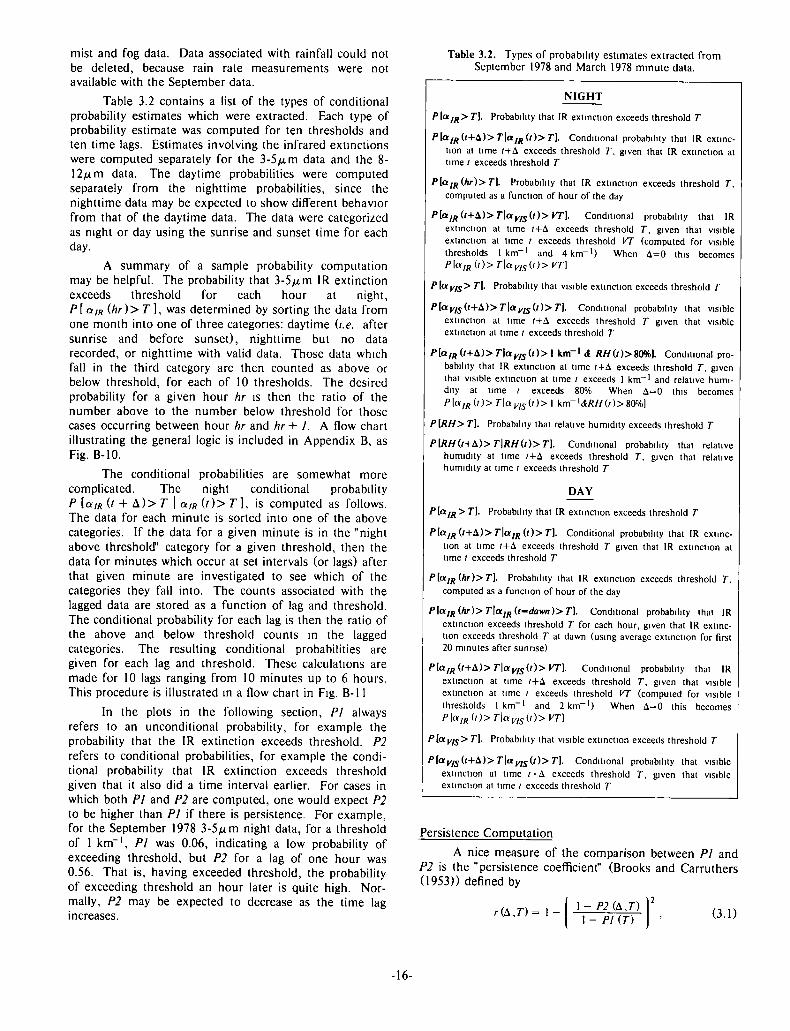
mist and fog data. Data associated with rainfall could not be deleted, because rain rate measurements were not available with the September data.

Table 3.2 contains a list of the types of conditional probability estimates which were extracted. Each type of probability estimate was computed for ten thresholds and ten time lags. Estimates involving the infrared extinctions were computed separately for the 3-5/j.m data and the 8-12/j,m data. The daytime probabilities were computed separately from the nighttime probabilities, since the nighttime data may be expected to show different behavior from that of the daytime data. The data were categorized as night or day using the sunrise and sunset time for each day.

A summary of a sample probability computation may be helpful. The probability that 3-5/xm IR extinction exceeds threshold for each hour at night, P[am (hr)> T], was determined by sorting the data from one month into one of three categories: daytime (i.e. after sunrise and before sunset), nighttime but no data recorded, or nighttime with valid data. Those data which fall in the third category are then counted as above or below threshold, for each of 10 thresholds. The desired probability for a given hour hr is then the ratio of the number above to the number below threshold for those cases occurring between hour hr and hr+ 1. A flow chart illustrating the general logic is included in Appendix B, as Fig. B-10.

The conditional probabilities are somewhat more complicated. The night conditional probability P [aiR (t + A)> T | am (t)> T], is computed as follows. The data for each minute is sorted into one of the above categories. If the data for a given minute is in the "night above threshold" category for a given threshold, then the data for minutes which occur at set intervals (or lags) after that given minute are investigated to see which of the categories they fall into. The counts associated with the lagged data are stored as a function of lag and threshold. The conditional probability for each lag is then the ratio of the above and below threshold counts in the lagged categories. The resulting conditional probabilities are given for each lag and threshold. These calculations are made for 10 lags ranging from 10 minutes up to 6 hours. This procedure is illustrated in a flow chart in Fig. B-l 1

In the plots in the following section, PI always refers to an unconditional probability, for example the probability that the IR extinction exceeds threshold. P2 refers to conditional probabilities, for example the condi­tional probability that IR extinction exceeds threshold given that it also did a time interval earlier. For cases in which both P1 and P2 are computed, one would expect P2 to be higher than PI if there is persistence. For example, for the September 1978 3-5/xm night data, for a threshold of 1 km-1, PI was 0.06, indicating a low probability of exceeding threshold, but P2 for a lag of one hour was 0.56. That is, having exceeded threshold, the probability of exceeding threshold an hour later is quite high. Nor­mally, P2 may be expected to decrease as the time lag increases.

Table 3.2. Types of probability estimates extracted from September 1978 and March 1978 minute data.

NIGHT

P[alR>T]. Probability that IR extinction exceeds threshold T

Pla,R(t+b)>T\aIR(t)>T]. Conditional probability that IR extinc­tion at time f+A exceeds threshold T, given that IR extinction at time t exceeds threshold T

P{alR(hr)>T]. Probability that IR extinction exceeds threshold T, computed as a function of hour of the day

PlalR(t+b)>T\am(t)>VT]. Conditional probability that IR extinction at time /+A exceeds threshold 7\ given that visible extinction at time I exceeds threshold VT (computed for visible thresholds 1km - 1 and 4 km-1) when A=0 this becomes PlaIR(i)>Tiayls(r)>VT]

P[ay/S> T]. Probability that visible extinction exceeds threshold T

PlayiS(t+\)>T\av[s(t)>T). Conditional probability that visible extinction at time r+A exceeds threshold T given that visible extinction at time i exceeds threshold T

P[aIR(t+&)>T\ay,s(.t)>l km - 1 it R//(/)>80%). Conditional pro­bability that IR extinction at time ;+A exceeds threshold 7", given that visible extinction at time ; exceeds 1 km -1 and relative humi­dity at time I exceeds 80% When A=0 this becomes P[aIRU)>T\am(i)>\ km-l&RH(r)>Sm)

P\RH> T\. Probability that relative humidity exceeds threshold 7"

P\RH(t+\)>T\RH(t)>T]. Conditional probability that relative humidity at time (+A exceeds threshold T, given that relative humidity at time I exceeds threshold T

DAY

P\f*lR > 71. Probability that IR extinction exceeds threshold T

P{alR(t+\)>T\aIR{t)>T]. Conditional probability that IR extinc­tion at time r+A exceeds threshold T given that IR extinction at time / exceeds threshold T

PlaIR(hr)>T]. Probability that IR extinction exceeds threshold 7", computed as a function of hour of the day

P[a,R(hr)>T\aIR(t-dawn)>T]. Conditional probability that IR extinction exceeds threshold T for each hour, given that IR extinc­tion exceeds threshold T at dawn (using average extinction for first 20 minutes after sunrise)

PlalR(l+£L)>T\otyls(t)> VT]. Conditional probability that IR extinction at time f+A exceeds threshold T, given that visible extinction at time I exceeds threshold VT (computed for visible thresholds 1km"1 and 2 km-1) When A=0 this becomes P\otIR(t)>T\avls(t)>VT]

P[<xVIS> 71. Probability that visible extinction exceeds threshold T

PlatyIS(t+b)>T\ayls(t)>T]. Conditional probability that visible extinction at time t+^ exceeds threshold 7\ given that visible extinction at time i exceeds threshold T

Persistence Computation

A nice measure of the comparison between PI and P2 is the "persistence coefficient" (Brooks and Carruthers (1953)) defined by

r ( A r ) ~ l - | ' - « < * . n 2 ( 3 1 )

-16-

where A is time lag, and T is threshold This coefficient ranges from +1 to — °°

Total persistence implies that once an event occurs it will definitely occur at the later time, thus PI would be less than 1, P2 would equal 1, and r would equal 1 No persistence is when the occurrence of an event has no effect on the probability of occurrence after the interval In this case, P2 would equal PI, so r would be 0 Nega­tive persistence results from the case where once an event occurs, it is less likely to occur after the interval In the extreme case, P2 would equal 0, and r would be a large negative number with magnitude depending on PI, the larger the PI value, the more negative r would be

Our use of the persistence coefficient is slightly different from the classical use Persistence normally requires that the event occur continuously during any prescribed time interval In our computations, P2 is the probability that the event occurs again Our P2 includes the cases in which the event was persistent (/ e continu­ous), intermittent, and recurrent (/ e occurred again for the first time at the end of the interval) Unfortunately, there appears to be no term which classically implies exactly this probability Reoccurrence might be the best term to use, although it is not defined statistically For the purposes of this report we will use the terms reoc­currence and persistence interchangeably to describe the statistics we have extracted

Plots of persistence coefficient were generated for both the visible data and the infrared data as a function of threshold and lag Appendix B contains plots of most of the probability types listed in Table 3 2 The probability plots are discussed in the next section In the next sec­tion, general statements regarding the interpretation of the statistics are intended to apply to this data set The extent to which these observations apply to other months and locations is largely unknown

3.2 Results of Probability Computations

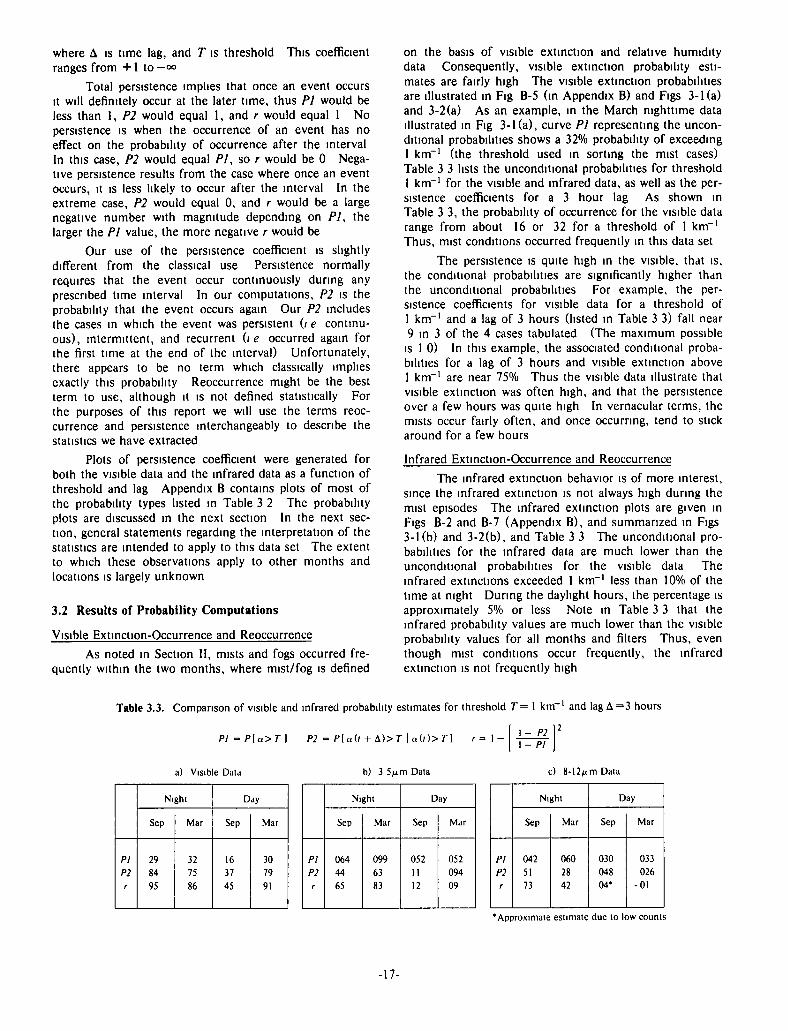
Visible Extinction-Occurrence and Reoccurrence

As noted in Section II, mists and fogs occurred fre­quently within the two months, where mist/fog is defined

on the basis of visible extinction and relative humidity data Consequently, visible extinction probability esti­mates are fairly high The visible extinction probabilities are illustrated in Fig B-5 (in Appendix B) and Figs 3-1(a) and 3-2(a) As an example, in the March nighttime data illustrated in Fig 3-1(a), curve PI representing the uncon­ditional probabilities shows a 32% probability of exceeding 1 km-1 (the threshold used in sorting the mist cases) Table 3 3 lists the unconditional probabilities for threshold 1 km-1 for the visible and infrared data, as well as the per­sistence coefficients for a 3 hour lag As shown in Table 3 3, the probability of occurrence for the visible data range from about 16 or 32 for a threshold of 1 km"1

Thus, mist conditions occurred frequently in this data set

The persistence is quite high in the visible, that is, the conditional probabilities are significantly higher than the unconditional probabilities For example, the per­sistence coefficients for visible data for a threshold of 1 km-1 and a lag of 3 hours (listed in Table 3 3) fall near 9 in 3 of the 4 cases tabulated (The maximum possible is 1 0) In this example, the associated conditional proba­bilities for a lag of 3 hours and visible extinction above 1 km-1 are near 75% Thus the visible data illustrate that visible extinction was often high, and that the persistence over a few hours was quite high In vernacular terms, the mists occur fairly often, and once occurring, tend to stick around for a few hours

Infrared Extinction-Occurrence and Reoccurrence

The infrared extinction behavior is of more interest, since the infrared extinction is not always high during the mist episodes The infrared extinction plots are given in Figs B-2 and B-7 (Appendix B), and summarized in Figs 3-1 (b) and 3-2(b), and Table 3 3 The unconditional pro­babilities for the infrared data are much lower than the unconditional probabilities for the visible data The infrared extinctions exceeded 1 km-1 less than 10% of the time at night During the daylight hours, the percentage is approximately 5% or less Note in Table 3 3 that the infrared probability values are much lower than the visible probability values for all months and filters Thus, even though mist conditions occur frequently, the infrared extinction is not frequently high

Table 3.3. Comparison of visible and infrared probability estimates for threshold T = 1 km ' and lag A =3 hours

2 Pl~P\a>T] P2 ~ P[a(t + b)>T \a(t)>T] r = l -

a) Visible Data b) 3 5/xm Data

1 - P2 1 - PI

c) 8-12/xm Data

Night Day Night Day Night Day

Sep Mar Sep Mar Sep Mar Sep Mar Sep Mar Sep Mar

PI

P2

r

29

84

95

32

75

86

16

37

45

30

79

91

PI

P2

r

064

44

65

099

63

83

052

11

12

052

094

09

PI

P2

r

042

51

73

060

28

42

030

048

04'

033

026

-01

"Approximate estimate due to low counts

-17-

Although the probability of the infrared extinction exceeding a high threshold is quite low, the probability of reoccurrence once such an event occurs (P2), about 50% at night, which is quite high (see Fig 3-1) The per­sistence coefficients given in Table 3 3 range from 4 to 8 for the night infrared data Although these values are not as high as observed in the visible data, they do yield fairly high conditional probabilities, as shown in the P2 curves of Fig 3-Kb) Thus, at night, once the infrared extinc­tion is high, it is likely to be high a few hours later also

The day infrared statistics (see Fig 3-2) are quite different from the night statistics As noted earlier, the probability of occurrence for 1 km-1 is much lower during the day The night and day probabilities differ the most at the higher thresholds, so that the higher threshold values are much more likely to occur at night Also, the reoc­currence probabilities are very low during the daytime The day persistence coefficients in Table 3 3 are approxi­mately 1, with associated conditional probabilities of reoc­currence of about 5-10% for the daytime infrared data During the daytime, therefore, the infrared extinction is unlikely to become high, and if it does become high, it is unlikely to remain high

Note in Fig 3-2 (b), that the P2 values for a 6 hour lag even fall below the PI values at high thresholds If a high extinction occurs, it is generally morning or evening, so the statistics for 6 hours later will be afternoon, when a high extinction is unlikely, or night, when the data will not be included Thus P2 is less than PI for this case, corresponding to negative persistence

At night, the persistence coefficients do not depend strongly on the time lag, as illustrated in Fig 3-3 As a result, the conditional probabilities are much greater than the unconditional probabilities for all lags tested, i e up to 6 hours lag That is, the extinction six hours after a high extinction event is nearly as likely to be high as an extinc­tion one hour after the high extinction event During the daytime, the persistence values are strongly lag dependent, and the conditional probabilities were significantly greater than the unconditional probabilities only for lags of an hour or less Thus the probability of occurrence is higher than normal for only about an hour after a high daytime extinction

Thus these data show that even though mists are occurring frequently, the infrared extinction is not often

CO

o 06 0_

O O

06 O

e—

CD CC 03 O 06

SYMBOLS - PI - P2(lflB 16) - P2ILH8 60) - P2tlP,S 1B0) - P2ILP.G 360

1 0 4 0 6 0 8

THRESHOLD EXTINCTION 0 2 04 06 08 10

THRESHOLD EXTINCTION (K.M-

Fig. 3-1 Visible probability estimates, PI = P[ayls> T] P2 =P[avls (f+A)> 7"] , and infrared 3-5^m probability estimates, PI =P[a,R>T),P2 =*P[a,R(t+A)>T \aIR(t)>T] March 1978, nighttime data

CD O 06

O

06 O

CO <n CO o or 0_

(a) Visible extinction SYMBOLS

o - PI o - P2IIA8 16) A - P2ILP.8 60) + - P2ILH6 180) X - P2ILH8 360)

CD O C£ 0_

o

0_ tr CQ o cc

1 0 4 0 6 0 8 10

THRESHOLD EXTINCTION

(b) 3 5 im extinction SYMBOLS

D - PI o - P2ILHB 16) A - P2ILBS 60) + - P2ILHG 1B0) x - P2ILRS 360)

T " 1 2

KM-l)

— i — 0 6 C2 0 4 0 6 0 8 1 0 1 2 1 4

THRESHOLD EXTINCTION (KM-l) 1 6

Fig. 3-2. Visible probability estimates, PI =P[ayls>T], P2 = P[ay,s(t+b)>T] , and infrared 3-5/u.m probability estimates, PI =P[a,R > T], P2 =P[a,R (M-A)> T | alR (t)> T] March 1978, daytime data

-18-

LJ O

LJ

z

to LJ

1 —

0.0 60.0 — I 1 1

120.0 180.0 240.0 LAG IN MINUTES

— i 300.0 360.0

LJ O CJ

CJ z L J e— CO

to en LJ Q_

1 r -

(b) Daytime data.

SYMBOLS T-0 .7 T-0 .9 T-1 .0 T-1.1 T-1 .3 T - l . S

CO 60.0 1 2 0 . 0 1 8 0 . 0 2 4 0 . 0

LAG IN MINUTES 300.0 360.0

Fig. 3-3. Persistence coefficients as a function of time lag, March 1978 3-5/j.m, where r = 1 - [(1 andP2 =P[aiR(t+b)>T \a,R(t)>T].

•P2)I(\-P1)V\ PI = Pla,R>T)

very high. Once it becomes high, it persists well at night, but very little during the day. The resulting conditional probabilities are much higher at night than during the day.

The unconditional probabilities for the infrared data were sorted as a function of hour of the day and are shown in Appendix Figs. B-l and B-6. For the thresholds of interest, the probabilities tend to be quite low during the daylight hours, then rise slightly during the night. The probabilities tend to be highest near dawn. Dawn occurred during the 05 hour in September, and the 05 and 06 hour during March. The September data show a definite increase in probability of occurrence during the before-dawn data at hour 04 and the after-dawn data dur­ing hour 05, while the March data have increased proba­bility values in the before-dawn data during hour 06. A sample of the plots is shown in Fig. 3-4. Note in Fig. 3-4(a) the rise at hour 04. The pre-dawn maximum is illustrated in Fig. 3-4(b) by the curve for hour 04, which lies above the curves for the other hours at all thresholds.

Infrared Extinction Occurrence After a Visible Event

Since the infrared extinction is related to the visible extinction as shown in Section II, it is desirable to try

using the visible extinction as a predictor. This kind of information is particularly useful, since visible extinctions in the form of visibility estimates are so readily available in the field. For this reason, estimates were extracted of the conditional probability that the infrared extinction exceed threshold, given that the visible extinction exceeds a given threshold. These estimates were extracted using the visible extinction thresholds of 1 km-1 and 4 km"1

during the night, for a range of infrared extinction thres­holds. During the daytime, there were not enough occurrences of 4 km-1 visible extinctions to yield reliable statistics, so visible extinction thresholds of 1 km-1 and 2 km-1 were used. The resulting plots are shown in Appendix Figs. B-3, B-4, B-8, and B-9.

These figures show that the conditional probability of occurrence, given the visible extinction exceeds 1 km-1, is higher than the unconditional probability of occurrence. Figure 3-5 shows an example of this. Comparing the con­ditional probabilities P[a/R 0+A)> T \am(t)>\ km - 1] , plots (c) and (d), with the unconditional probabilities Pla/R > T ], which are the PI curves in plots (a) and (b), one can see that a high infrared extinction is more likely to occur if the visible extinction has recently exceeded 1 km"1.

—> oo

( > o X T f 1

x LJ rn < i «• 0_ o

n z o o o

(a) Unconditional probability vs hour.

SYMBOLS O - T-0.7 o - T-0.9 a - T-1.0 + - T-1.1 X - T-1.3 0 - T-l.S

ID O X

o CE

£ »•

CO X CO

o

10.0 12.0 14.0 16.0 18.0 2 0 . 0 2 2 . 0 24 .

HOUR 0.4 0 .6 0 .6 1.0

THRESHOLD EXTINCTION

Fig. 3-4. Unconditional probability each hour, P[aIR (hr)> 71. September 1978, 3-5/*m nighttime.

•19-

\

SYMBOLS D - PI O - P2ILRB 16) a - P2(lflG 60 + - P2ILHG 180 X - P2ILRB 360)

-r- — I — 0 . 4

—I 0.6

—r~ 0.8 I 0 . 2 0 .4 0 .6 0 .8 1.0

THRESHOLD EXTINCTION

(a) Nighttime PI = Pla/R>T\

1.2 1.4

(KM-1) 1.6

CO o ce

o o

m x CO

o Q_

SYMBOLS D - PI o - P2ILAG 16) i - P21LRG 60) + - P2IIRG 180) x - P2ILRG 360

P2 = P{aIR(.t+b)>T \aIRU)>T)

0.0 0.2 0 4 0.6 0.8 1.0 1.2

THRESHOLD EXTINCTION (KM-1)

(b) Daytime PI = P[aIR>T] P2 = P[aIRU+CL)>T \a,RU)>T)

0.4 0.6 0.8 1.0

THRESHOLD EXTINCTION

x. o

o

(c) Nighttime P[aIR (r+A)> T | aylsU)> 1 km-1]

0 .4 0 .6 0 . 8 1.0 1.2

THRESHOLD EXTINCTION (KM-1)

(d) Daytime P[a,R(t+A)>T \ avlsU)> \ km

0.0

SYMBOLS - P2ILR6 0) - P2ILAS 16) - P2ILRG 60) - P2IIRG 1B0)

—I 0.2

-1 0.4 0.6

-1 0.8

-1 1.0

-1 1.2

-1 1.4

THRESHOLD EXTINCTION (KM-1) (e) Nighttime P\ot/R ('+A)> 7" | a y/sU)> 4 km -

1.6

03 SYMBOLS o " O - LRG-0

o - LRG-16 4 - LRG-60

UJ + - LAG-180

(_) "? X - LflG-360 I t U-

n s • « *

( > o °

0 . 0 0 . 2 0 .4 0 .6 0 .8 1.0 1.2

THRESHOLD EXTINCTION (KM-1)

(f) Daytime Pk*iR ('+A)> T I a yfs(i)> 2 km -

Fig. 3-5. Comparison of conditional probabilities resulting from IR extinction conditions with those resulting from visible extinction con­ditions September 1978, 3-5^m

Tables 3.4 and 3.5 illustrate these results for the infrared extinction threshold 1 km-1. Comparing the unconditional probabilities in the first row with the condi­tional probabilities in rows 4 and 5, one can see that the conditional probabilities given that the visible extinction

exceeded 1 km ' are somewhat higher than the uncondi­tional probabilities, for both seasons and filters.

Interestingly, these conditional probabilities do not depend strongly on the time lag at night, up to lags of at

-20-

least 6 hours. This effect is simply the result of the high persistence in the visible extinction. During the daytime, the conditional probabilities are strongly lag dependent. The dependence on lag is illustrated in Fig. 3-6.

Whereas the conditional probability P[a,R ( r+A)> T | aviS{t)> 1 km - 1 ] is greater than the unconditional pro­

bability P[a/R > T ] , we find that at night it is much lower than the P[ a,R (f+A)> T \a,R(t)>T] conditional proba­bilities discussed earlier. This may be seen from a com­parison of rows 2 and 3 with rows 4 and 5 of Tables 3.4 and 3.5, or from a comparison of the P2 curves of plot (a) with the curves of plot (c) in Fig. 3-5. Note that at night an infrared event 6 hours in advance is associated with higher conditional probabilities than even a simultaneous visible event.

For the daytime data, the P[a,R 0 + A ) > T \awS(t)>\ km - 1 ] conditional probabilities are compar­

able in magnitude to the P[a,R (r+A) > T \a,R(t)>T] conditional probabilities for A values of more than an hour. That is, the conditional probabilities associated with an earlier visible extinction event are about equal to the conditional probabilities associated with an earlier infrared event during the day, if the lag is more than an hour. Only for a time lag of an hour or less is the P[a/R (f+A) > T | atR U)>T] conditional probability significantly greater. Thus, the infrared extinction lis more likely to exceed threshold if the visible extinction exceeds thres­hold 1 km - 1 simultaneously or earlier. That is, the condi­tional probabilities are higher than the unconditional pro­babilities. And at night it is even more likely to exceed

Table 3.4. Effect of visible vs infrared conditions on probability estimates, for threshold 7"=1 krrr1 September 1978 data

Table 3.5. Effect of visible vs infrared conditions on probability estimates for threshold 7*= 1 krrr1, March 1978 data

Probability Type Nighl Day

Probability Type 3-5^11 8-12Mm 3-5/im 8-12Mm

Unconditional P1 a /R > T1

T - 1 k m - ' 064 042 052 030

Conditional on Infrared

P\aIR(t+b)>T \aIR{i)>T]

T~ 1 k m - 1 , A - 6 h r 33 31 057 037

T- 1 km"1 . A - 1 hr 56 55 28 25

Conditional on Visible

PlaIRU+b)>T \a„lsU)>VT\,

T-\ km"1

VT- 1 k m - 1 , A - 6 h r 17 07 065 040

VT- 1 k m - 1 , A - 0 20 14 26 17

VT- 4 or 2* k m - 1 , A - 3 hr 81 46 095 044

VT - 4 or 2* km"' , A - 0 78 47 47 32

Probability Type Nighl Day

Probability Type 3-5^m 8- l2 M m 3-5nm 8- l2 M m

Unconditional P1 a [R > T1

T = 1 k m " '

Conditional on Infrared

/ > t a / w ( H - A ) > 7 " \aIRU)>T]

T= 1 k m " 1 . A = 6 h r

T= 1 k m " ' , A = 1 hr

Conditional on Visible

/ > U / R ( f + A ) > r \amU)> VT].

T=\ k m " 1

VT = 1 k m " 1 , A = 6 h r

VT = 1 k m " ' . A = 0

VT- 4 or 2* k m - 1 . A = 3 hr

VT = 4 or 2* k m " ' . A = 0

099

64

71

30

29

86

91

060

42

58

19

18

69

59

052

061

38

093

15

063

34

033

< 015

30

040

093

009

222

•Used 4 for nighl, 2 for day •Used 4 for nighl, 2 for day

03 O

a:

o 1 k ^

1 1 1 r (a) Nighttime data, Sep 3-5/j.m

SYMBOLS D - T-0.7 o - T-0.9 a - T-l .O + - T - l . l X - T - l . 3 0 - T - l . S

•ae-e-

0.0 60.0 120.0 180.0 240.0 300.0

LRG IN MINUTES 360.0

CD O or o_ a a CJ

-i 1 1 1 r (b) Daytime data, Sep 3-5/* m

0.0 60.0 120.0 180.0 240.0 300.0 LAG IN MINUTES

360.0

Fig. 3-6. Conditional probabilities, P\aiR 0+A)> T I amd)> l km -1], as a function of time lag September 1978, 3-5/im

-21-

threshold if the infrared extinction exceeds threshold even as much as 6 hours earlier.

When the visible extinction threshold used in the conditional requirement is increased, the conditional pro­babilities are significantly increased. Plots (e) and (f) of Fig. 3-5 show the conditional probabilities P[aIR 0+A) >T | avls(t)>4 km-1] for nighttime and P[a,R (t+\) >T | ayis(t)>2 km -1] for daytime, respectively. Also see rows 6 and 7 of Tables 3.4 and 3.5. The probabilities are quite high, being comparable to the P[a,R 0+A) >T | amU)>T ] probabilities for a lag of 16 minutes. The daytime data probabilities were extracted for visual threshold 2 km-1 rather than 4 km-1 due to lack of data. These conditional probabilities are much higher than those for visible extinction threshold 1 km-1, being similar in magnitude to the P[a,R (t+&)> T \aIR(t)>T] probabil­ities in plot (b).

The P[a,R(t+A)>T | a r a 0 ) > 4 k m - ' ] probabili­ties do not depend strongly on lag during the night, as shown in Fig. 3-7. The daytime P[aIR (t + A)> T I aviS(t)>2 km-1 ] probabilities are strongly lag depen­dent.

To summarize, if one is trying to predict whether the infrared extinction is going to exceed threshold, know­ing that the visible extinction is quite high, say > 4 km-1, is a good indicator. However, when the visible extinction is somewhat lower however, for example near 1 km-1, then a measurement of the infrared extinction provides a better indicator than a measurement of visible extinction. Knowing that the infrared extinction is high is a good indi­cator for several-hour forecasts at night.

Additional Probability Estimates

The data were also used to extract the conditional probability of exceeding threshold given that the visible extinction exceeded 1 km"1 and the relative humidity exceeded 80%. These conditional probabilities, P[aIRU+A)>T \am(t)>\ km"1 & RH(t)>80%], are quite similar to the conditional probabilities given visible extinction > 1 km-1, P[a,R (/+A)> T\ay,s(t)> 1 km"1].

A typical sample of the effect of the relative humi­dity condition is illustrated in Fig. 3-8. In this figure, the plot (b), which shows P[a,R (t+A)>T \ ay,s(t) > l k m - ' c 5 RH(.t)>&0%] is nearly identical to plot (a), which shows P[a,R 0+A)> T | a r a 0 ) > 1 kirr1 ]. Some similarity is to be expected, because the relative humidity normally exceeds 80% when aVIS exceeds 1 km-1; roughly }A of the cases with a r a > 1 km-1 also have RH> 80%. The major cause of the similarity in the statistics, how­ever, is the high persistence of the relative humidity values. Plot (c) shows the conditional probabilities for relative humidity, P[RH(t+A)> T \ RH(t)> T]. For relative humidity values of 80%, the persistence is very high, being .98 for a six hour lag in September at night. This high persistence is the reason that imposition of the relative humidity condition has little additional effect. Higher relative humidity values persist about 4 hours.

There are additional probability estimates which would be of interest, however with a one month data sam­ple, lack of data can become a problem. Each additional condition which is imposed on the data eliminates addi­tional data cases and thus lowers the number of values considered. In particular, an attempt was made to extract the conditional probability that the infrared extinction would exceed threshold given that the infrared extinction exceeded threshold at dawn. Figure 3-9 shows a sample comparison of the effects of adding the dawn conditional requirement. Although the conditional probabilities in plot (b) are higher than the unconditional probabilities in plot (a), there were too few data points to yield accurate estimates. For example, for hour 12, threshold 1.0 km-1, the above and below threshold counts are 16 and 385 respectively for plot (a), and 2 and 43 respectively for plot (b). This lack of data is apparent in the increased scatter of plot (b).

3.3 Summary of Probability Estimate Results In general, the behavior of the extinction values, as

indicated by the probability estimates, is quite different at nighttime and at daytime. The two months of data which

oo CO or Q.

Q z o CJ

180.0 240.0 IN MINUTES

360.0

SYMBOLS T-0.7 T-0.9 T-1.0 T-1.1 T-1.3 T-1.5

(b) Daytime data

0.0 60.0 120.0 180.0 240.0 LAG IN MINUTES

300.0 360.0

Fig. 3-7. Conditional probabilities as a function of time lag PlaIR (H-A)> T | ay/s (/)> 4 km""1] at nighttime, P[a,R (t+A)>T | avls(t)> 2 km-1] during daytime March 1978, 3-5fxm

-22-

f -

CQ CC

o o : o_

CC' •<•

o 2 O CJ

SYMBOLS • - P2ILA0 0) o - P2[LflS 16) 4 - P2ILAB 60) + - P2ILRB 180) X - P2ILRB 360)

(r+A)>r \ayiS(l)> 1 km

0.0 — 1 1 1 1 1 1 I 0.2 0.4 0.6 0.8 1.0 1.2 1.4

THRESHOLD EXTINCTION (KM-1)

CO cc CD o "> CC o"' o_

cc •«•

o CJ

SYMBOLS D - P2ILHS 0)

>a- P2(LflB 16) n - P2IUW 60) + - P2tlflB 180) X - P2ILP.B 360)

(b) Pla,R(t+b)>T \c,yls(l)> 1 km"

&RH{l)> 80%]

1 1 1 1 1 - I 1 —

0.0 0.2 0.4 0.6 0.8 1.0 1.2 1.4 THRESHOLD EXTINCTION (KM-1)

50.0 60.0 70.0 80.0 90.0

THRESHOLD REL HUM ("/.) 100.0

Fig. 3-8. Effect of adding a relative humidity conditional requirement. September 1978, 3-5/Lim, nighttime.

or O X X o en >-t—

CQ CC CO o o; a.

(a) P[aIR(hr)>T]

SYMBOLS a - T-0.7 o - T-0.9 & — T-1.0 + ~ T-1.1 x -o —

T-1.3 T-l.S

f • f

~* l 1 i i 1 — i i I I I

^ » (b) Pic, m Uir)>T\alR(dawn)>T] O <=" ~ X

O "> CC a-Ul CD O f

SYMBOLS a- 1-0.7 o - T-0.9 a - T-1.0 + - T-1.1 X - T-1.3 » - T-l.S

a

CJ a /S -o

r * f * t T T 1 0.0 2.0 4.0 6.0 8.0 10.0 12.0 14.0 16.0 18.0 20.0 22.0 24.0

HOUR 0.0 2.0 4.0 6.0 8.0 10.0 12.0 M.O 16.0 19.0 20.0 22.0 24.0

HOUR

Fig. 3-9. Effect of adding the conditional requirement that extinction exceed threshold at dawn. September 1978, 3-5/xm, daytime.

were extracted yielded values which were quite similar in behavior, although somewhat different in magnitude in some cases.

In this data set, the overall probability of having high extinction values was fairly high in the visible region, but quite low in both infrared bands. The persistence is very high in the visible region. In the infrared bands, the persistence at night is high, although not quite so high as in the visible. The resulting conditional probabilities at

night are high, for lags up to at least 6 hours. During the day, the persistence is high only for a lag of about an hour or less. After an hour, the conditional probabilities in the infrared regions become very low during the day.

Conditional probabilities based on the visible extinc­tion as a conditional requirement were also computed. The resulting conditional probabilities P[am (t+A)> T \ay/sU)>\ km - 1 ] were in general not as high as the P[a/R 0 + A ) > T | a,R 0 ) > T ] conditional probabilities.

-23 -

In the rare cases when the visible extinction exceeded 4 km-1, however, infrared conditional probabilities became very high.

It is not clear yet whether it will eventually be possi­ble to parameterize these relationships in an operationally useful way. The general behavior of the two months' data is so similar that there is reason to try to quantify these relationships. An additional 10 months of data is currently undergoing processing. These additional data will allow us to investigate the month-to-month changes, as well as introduce additional conditional requirements. For example, air mass type, predicted fog type, the number of hours the mist has already persisted, and the rate of temperature drop are additional predictors which could perhaps be evaluated with the larger data base. It would be particularly useful if the data yield consistent conditional probability data as a function of the visible extinction, since predicted visible extinctions are often available in the field.

4.0 CONCLUSION

This report discusses an analysis of atmospheric extinction coefficients measured simultaneously in the visible and infrared (3-5/j,m and 8-12^m) regions. The measurements, taken in Meppen Germany, were recorded at one minute intervals. Of the year's data base which is currently available, this report discusses the analysis of two months of data.

The analysis was designed to evaluate the short term temporal variations in the infrared extinction coefficient, particularly during mist and fog episodes. Previous research based on hourly interval data indicates that the relation between the infrared and visible extinction can be quite variable under these conditions. The variations in the hourly data appear to be occurring on a time scale which is short relative to the length of the mist episodes. The minute data were analyzed because they are uniquely suitable for studying the nature of the short term temporal variations and for extracting statistics relating to the pro­bability that the infrared extinction will become high and remain high.

4.1 Results of the Analysis

Mist Bin

It was found that the high infrared aerosol extinc­tions in the minute data set tend to occur only when the visible extinction exceeds 1 km-1 and the relative humi­dity exceeds 80%. The set of points meeting these condi­tions were defined as the mist bin. Within this mist bin, which includes both mist and fog, the infrared extinction data are quite variable. The ratio of infrared aerosol to visible extinction was found to cover a large range of values, even at the high visible extinction values normally associated with fog (about 4 km-1 or more).

Extinction Relations During Mist Episodes

In order to understand the nature of this variation, continuous mist or fog periods lasting 30 minutes or more

were extracted and studied in more detail. Plots of the infrared aerosol extinction and visible extinction as a func­tion of time during the mist episodes were generated, along with plots of infrared aerosol extinction as a func­tion of visible extinction.

During some mist episodes, temporal variations in the infrared aerosol extinction corresponded very well to the variations in the visible extinction. In a few episodes, the infrared and visible extinctions appeared to be unre­lated. In many cases, the infrared extinction variations corresponded well to the visible extinction variations, except that they were very much magnified. That is, a small change in visible extinction often was associated with a very large change in infrared aerosol extinction. Also, in many cases the infrared extinction had essentially no variation as long as the visible extinction was below a certain threshold value; when the visible extinction was above that threshold value, the infrared extinction showed very large excursions in conjunction with the visible extinction changes. The visible threshold at which this behavior occurred tended to vary from one episode to the next. Although this threshold-type behavior occurred dur­ing several mist episodes, there were several other mist episodes, with similar values of visible extinction, which did not show any threshold-type behavior.

During the mist episodes, the infrared aerosol extinctions were related to the visible extinctions in a nearly linear manner during approximately half the episodes. Thus it was found that although some of the variability in the infrared to visible relationship in the mist bin is due to differences between the individual mist episodes, much of the variability may be attributed to vari­ation in the infrared-visible relationship within individual mist episodes. The magnified changes in the infrared extinction occurring within a mist episode in conjunction with relatively small visible extinction changes (discussed in the previous paragraph) particularly contributes to this variation in the infrared-visible relationship.

Probability Results

Following the above analysis of mist and fog periods, statistics relating to the probability of a high infrared extinction occurring were discussed. For this analysis, the complete data base for each of the two months was used, rather than just the mist bin, and the total extinction rather than the aerosol extinction was used. It was found that although the visible extinction exceeded thresholds on the order of 1 km-1 fairly often, the infrared extinction exceeded such thresholds only rarely. For the higher thresholds, the infrared extinction was particularly unlikely to exceed threshold during the daylight hours.

Although high extinction events were infrequent, it was found that once a high infrared extinction occurred, it was quite likely to remain high, particularly during the night hours. That is, the conditional probability that the infrared extinction will exceed threshold a given interval after it has once exceeded threshold was quite high, for intervals up to at least 6 hours at night. The associated

-24-

persistence coefficients were therefore high. During the daylight hours, the persistence and associated conditional probabilities were high only for an interval of approxi­mately an hour. After an hour, the conditional probabili­ties were quite low.

Although the infrared extinction persistence was high at night, it was not as high as the nighttime per­sistence in the visible extinction coefficient. That is, the high infrared extinction values were less stable than the high visible extinction values.

It was also found that once a high visible extinction occurs, a high infrared extinction is somewhat more likely to occur. That is, the conditional probability that the infrared extinction will exceed threshold a given interval after the visible extinction has exceeded some threshold is somewhat higher than the unconditional probability that the infrared extinction will exceed threshold. This effect is nearly lag (or interval) independent, for intervals of at least 6 hours. When the visible extinction used in the conditional requirement is increased, the conditional pro­babilities for high infrared extinction increase consider­ably.

In summary, the probability estimates show that if a high infrared extinction occurs, the infrared extinction has a fairly large probability of exceeding threshold in subse­quent hours, particularly at night. Also, if a high visible extinction occurs, the infrared extinction has a more than normal probability of exceeding threshold in subsequent hours--in fact the probability becomes fairly large if the conditional visible extinction is increased. In general, however, the overall probability of a large infrared extinc­tion occurring is quite low.

Although the magnitudes of the extracted probabil­ity estimates differed somewhat on the two months, the general character of the probability curves was quite simi­lar. The behavior of the night data differed considerably from the behavior of the day data.

4.2 Continuing Analysis Objectives

The additional 10 months of minute data are currently undergoing processing and initial quality evalua­tion. With this larger data base, it should be possible to introduce additional predictors and conditional require­ments on. the data. Although the exact approach to the data analysis has not yet been established, there are several approaches which are being considered. Depend­ing on data availability, it may be possible to sort the data and determine conditional probabilities for different air mass types, and/or for different fog types. Another sort­ing criteria of interest is the length of time that the high extinction has already persisted, and perhaps the rate at which the temperature dropped. Months will probably be combined seasonally for this analysis.

The hope is that if the important predictors can be determined, it may be possible to yield repeatable proba­bility estimates. That is, if the data are sorted on the basis of season and fog type, for example, or perhaps visibility predicted by the weather service, it may be that indepen­

dent data sets, say in two different months, will yield con­sistent conditional probability estimates. If this were the case, these relationships could perhaps be parameterized for forecasting. On the other hand, if the real world data fall short of this hope, it could be operationally useful to determine the general data relationships, and how these relationships vary from month to month.

In addition to further analysis of probability esti­mates, mentioned above, continuing analysis of the mist and fog episode data is planned. As noted in Section 2, the infrared extinction is sometimes stable and/or well related to visible extinction during the mist episodes, and sometimes it is extremely variable. The ability to predict which type of behavior will occur in an ongoing mist or fog episode would be operationally important. With this goal in mind, we particularly wish to investigate rain data and aerosol particle distribution measurements when they are available during mist periods.

5.0 REFERENCES

Brooks, C.E.P., and N. Carruthers (1953), Handbook of Statistical Methods in Meteorology, Air Ministry, Meteorological Office, Her Majesty's Stationary Office, London.

Fenn, R.W. (1978), "OPAQUE - A Measurement Program on Optical Atmospheric Properties in Europe, Vol. I. The NATO OPAQUE Program", Special Reports No. 211, AFGL-TR-78-0011, ADB 029 877L.

Fenn, R.W., T.S. Cress, Dr. DeHart, R. Dirkman, J.D. Essex, K. Lichtenberg, V.A. Marcello, J.E. Powers, E.P. Shettle, H. Soron, J. Sullivan, F.P. Suprin, R.B. Toolin, V.D. Turner, F.E. Volz (1979), "OPAQUE -A Measurement Program on Optical Atmospheric Quantities in Europe, Vol. II - The US/German OPAQUE Station Near Meppen, Federal Republic of Germany", Special Reports No. 222, AFGL-TR-79-0068, ADB 045 111L.

Gimmestad, G.G., L.W. Winchester, Jr., W.K. Choi, and S.M. Lee (1982), "Correlation Between the Infrared and Visible Extinction Coefficients of Fog", Optics Letters, Vol. 7, No. 10, 471-473.

Huschke, R.E. (1976), "Atmospheric Visual and Infrared Transmission Deduced from Surface Weather Obser­vations: Weather and Warplanes VI", Report R-2016-PR RAND, Santa Monica.

Janssen, L.H. and J. van Schie (1982), "Frequencies of Occurrance of Transmittances in Several Wavelength Regions during Three Years", Appl. Opt., Vol. 21, No. 12, 2215-2223.

Kneizys, F.X., E.P. Shettle, W.O. Gallery, J.H. Cherwynd, Jr., L.W. Abreu, J.E.A. Selby, R.W. Fenn, and R.A. McClatchey (1980), "Atmospheric Transmittance-Radiance Computer Code LOWTRAN5", AFGL-TR-80-0067, ADA 088 215.

Kohnle, A. (1979), "Barnes Calibration via LOWTRAN, some Aspects", Forschunginstitut fur Optik, Tubingen, OPAQUE AN-N/GE-7908.

-25-

Mcintosh, D.H. (1963), Meteorological Glossary, Meteoro­logical Office, Her Majesty's Stationary Office, Lon­don.

Nilsson, B. (1979), "Meteorological Influence on Aerosol Extinction in the 0.2-4.0/XWJ Wavelength Range", Appl. Opt., Vol. 18, No. 20, 3457-3473.

Proulx, G.J. (1971), Standard Dictionary of Meteorological Sciences, Scientific and Technical Division, Depart­ment of the Secretary of State, Ottawa, Canada, McGill-Queen's University Press.

Shand, W.A. Ed. (1978), "Barnes Intercomparison Trial-Pershore. September 1977", RSRE(C) Christchurch, Dorsett, England, OPAQUE R7804.

Shettle, E.P. (1978a), "Theoretical Transmittances for the OPAQUE Barnes Transmissometers", Air Force Geophysics Laboratory, Bedford, Mass., OPAQUE N/US-7805.

Shettle, E.P. (1978b), "Analytic Expressions for the Atmospheric Water Vapor Content", Air Force Geo­physics Laboratory, Bedford, Mass., OPAQUE N/US-7810.

Shettle, E.P. (1980), "Procedure for Calibration of the OPAQUE IR Transmissometers via LOWTRAN Cal­culations", Air Force Geophysics Laboratory, Bed­ford, Mass., OPAQUE N/US-8001.

Shettle, E.P. and R.W. Fenn (1978), "IR-Transmissometer Calibration, Comparison with LOWTRAN', Air Force Geophysics Laboratory, Bedford, Mass.,

• OPAQUE N/US-7808. Shettle, E.P. and R.W. Fenn (1979), "Models for the

Aerosols of the Lower Atmosphere and the Effects

of Humidity Variations on Their Optical Properties", AFGL-TR-79-0214, ADA 085 951.

Shields, J.E. (1981), "An Analysis of Infrared and Visible Atmospheric Extinction Measurements in Europe", University of California, San Diego, Scripps Institu­tion of Oceanography, Visibility Laboratory, SIO Ref. 82-4, AFGL-TR-81-0251, ADA 123 999.

6.0 ACKNOWLEDGEMENTS This report has been prepared for the Air Force

Geophysics Laboratory under Contract No. F19628-82-0060. I wish to thank the members of the Atmospheric Optical Physics Optics Branch of the Air Force Geophysics Laboratory, who supplied the data, and provided technical support. Special thanks to Mr. Eric Shettle for his help with the data quality evaluations. Credit is due to the Air Force Geophysics Laboratory, Mr. K. Lichtenberg and personnel from the Meppen Artillery Test Range, Meppen Germany, who were jointly responsible for the measure­ment program.

Several members of the Visibility Laboratory staff have been most helpful. I appreciate the assistance of the following individuals: Mr. Richard W. Johnson and Mr. Wayne S. Hering, for their valuable discussions during the analysis stages; Ms. Miriam K. Oleinik, for advice and assistance with the computer program development stages; Ms. Alicia G. Hill, Mr. John C. Brown, and Mr. James Rodriguez for careful document preparation; and Mr. John S. Fox for assistance with computer processing.

-26-

APPENDIX A

Time Series Plots and Scatter '. and Visible Ex

This appendix contains most of the time series plots and scatter plots which were generated for the analysis in Section 2. Figures A-l through A-6 illustrate the infrared aerosol extinction coefficients and the visible extinction coefficients for each mist episode, plotted as a function of time since the beginning of the episode. Only the simul­taneous visible extinctions at 4 minute intervals were plot­ted. The episode start times are indicated in the figure captions. Plots such as A-4 (c) and (d), which are a con­tinuation of the previous plot, begin 800 min and 1600 min after the episode start. Figures A-7 through A-14 illustrate the plots of infrared aerosol extinction coefficient plotted as a function of visible extinction coefficient for each mist episode.

Plots were generated if there were at least 40 data points within an episode. In some cases the plots have not been included in this appendix because the infrared data are below the plotting scale minimum of .01 km-1. As a consequence, the number of plots included in this appen­dix is not exactly the same as the number of 3 hour

of Infrared Aerosol Extinction ion Coefficient

episodes listed in Table 2.1. Two episodes included in the time series plots (A-l through A-6) are deleted from the scatter plot figures (A-7 through A-14) because the numbers are mostly offscale in one case, and nearly con­stant in the other.

The sorting program requires that the visible extinc­tion and relative humidity be valid and above threshold throughout the whole episode. (The only exception to this rule is the case in which the visible data were not reported because the IR data were offscale.) In the mist episode of Fig. A-2(g,h) the visible extinction dropped below 1 km-1 during one 8-12 /w measurement at 1612, but remained above threshold during the 3-5/xw measure­ments. As a consequence, the 8-12 im data sort yielded a mist starting at 1616, whereas the 3-5/AW data sort yielded an earlier start time, 1534. In two other cases, A-l(a,b) and A-3(a,b) the mist start times differ for the two filters due to a momentary loss of visible extinction data in one filter's data set.

(a) 5 Sep 2320, 3 -5 / im (b) 5 Sep 2345, 8 -12^m

120.0 240.0 360.0 180.0 600.0 720.0 MINUTES SINCE EPISODE START

0.0 120.0 240.0 360.0 480.0 600.0 720.0 840.0 MINUTES SINCE EPISODE START

(c) 6 Sep 2110, 3 -5 / im (d) 6 Sep 2112, 8-12/*"!

120.0 240.0 360.0 480.0 600.0 720.0 840.0 MINUTES SINCE EPISODE START

0.0 120.0 240.0 360.0 480.0 600.0 720.0 840.0 MINUTES SINCE EPISODE START

(e) 7 Sep 1830, 3 -5 / im — --

- : (0 7 Sep 1836, 8-12/xm

»

u ^ r ^ en

2

L Jo_ I 1

1 1 1 * — 1 — • — i r" 1

120.0 240.0 360.0 480.0 600.0 720.0 MINUTES SINCE EPISODE START

0.0 120.0 240.0 360.0 480.0 600.0 720.0 840.0 MINUTES SINCE EPISODE START

(g) 9 Sep 0226, 3 - 5 ^ (h) 9 Sep 0228, 8-12/xm

120.0 240.0 360.0 480.0 600.0 720.0 MINUTES SINCE EPISODE START

0.0 120.0 240.0 360.0 480.0 600.0 720.0 MINUTES SINCE EPISODE START

Fig. A-l. September 1978, aerosol extinction vs time (D = < * V I S 0 = 0 : I R ) -

-28-

(a) 14Sep0858, 3-5Mm

120.0 240.0 360 0 480.0 600.0 720.0

MINUTES SINCE EPISODE START

—'. _ 1 (b) 14 Sep 0900, 8-12/im

T 1

EXTI

NC (KM

10'

* o . Q —: 2 cr a;

' o . " - I 1 1 1 1 1 1 120.0 240.0 360.0 480.0 600.0 720.0

MINUTES SINCE EPISODE START

(e) 20 Sep 2230, 3-5Mm (d) 20 Sep 2236, 8-12Mm 71

EXTI

NC (KM

10'

<n

O ~- :

-z. oc 1 •

'o ii i — ^ — i 1 1 1 1 1

120.0 240.0 360.0 480.0 600.0 720.0 840.0 MINUTES SINCE EPISODE START

0.0 120.0 240.0 360.0 460.0 600.0 720.0 840.0 MINUTES SINCE EPISODE START

(e) 22 Sep 0234, 3-5Mm

.vw

J

(f) 22 Sep 0228, 8-12M m

X CJJ

tr>

> 'a. a —': •z. a: ;

or

'o J\K r W / M i

0 0 120 0 240 0 360 0 480 0 600 0 720 0 840 0

MINUTES SINCE EPISODE START 120.0 240.0 360.0 460.0 600.0 720.0 840.0 MINUTES SINCE EPISODE START

—1 : (g) 22 Sep 1534, 3-5/x m

—

EXTI

NC (KM

10'

IR AND VIS

10° \ p

1 Hz 'o . 1 I , (U, , , ,

(h) 22 Sep 1616, 8-12/in

120.0 240.0 360.0 460.0 600.0 720.0 MINUTES SINCE EPISODE START

120.0 240.0 360 0 480.0 600 0 720.0 MINUTES SINCE EPISODE START

Fig. A-2. September 1978, aerosol extinction vs time ( o = a v t s 0 = a t R ^

-29-

o . a —

(a) 23 Sep 2332, i-Sfim -:

(b) 24Sep0038, 8-12Mm

V

,01

ON

11X3

S

a —*: CE

'o » ^ y r & - g ^ 0 ' A.-C- ^v^^-^^-g^e"-**—^"^

0.0 120.0 240.0 360.0 480.0 600.0 720.0 840.0 MINUTES SINCE EPISODE START

(c) 28 Sep 2334, 3-5Mm

0 0 120 0 240 0 860 0 480 0 600 0 720 0 840 0

MINUTES SINCE EPISODE START

(d) 28 Sep 2332, 8-12^ m

v^JA .ft 0.0 120.0 240.0 360.0 480.0 600.0 720.0 B40.0

MINUTES SINCE EPISODE START 120.0 240.0 360.0 480.0 600.0 720.0 840.0

MINUTES SINCE EPISODE START

Fig. A-3. September 1978, aerosol extinction vs time (D =a v , s O=o I R )

-30-

(a) 3 Mar 0935, i-5tim

0.0 120.0 240.0 360.0 480.0 600.0 720.0 840.0 MINUTES SINCE EPISODE START

(b) 3 Mar 0929, 8-12Mm

0.0 120.0 240.0 360.0 480.0 600.0 720.0 840.0 MINJTES SINCE EPISODE STPRT

(c) 3 Mar 0935, 3-5Mm cont.

0.0 120.0 240.0 360.0 480.0 600.0 720.0 840.0 MINUTES SINCE EPISODE START

(d) 3 Mar 0929, 8-12^ m cont.

120.0 240.0 360.0 480.0 600.0 720.0 MINUTES SINCE EPISODE START

(e) 3 Mar 0935, 3-5jim cont

D 2 or

0.0 120.0 240.0 360.0 480.0 600.0 720.0 840.0 MINUTES SINCE EPISODE START

(0 3 Mar 0929, 8-12Mm cont

0.0 120.0 240.0 360.0 480.0 600.0 720.0 840.0 MINUTES SINCE EPISODE START

(g) 5 Mar 0025, 3-5^™

0.0 120.0 240.0 360.0 480.0 600.0 720.0 840.0 MINUTES SINCE EPISODE START

(h) 5 Mar 0019, 8-12Mm

120.0 240.0 360.0 460.0 600.0 720.0 MINUTES SINCE EPISODE START

Fig. A-4. March 1978, aerosol extinction vs time (D *visk MR'

- 3 1 -

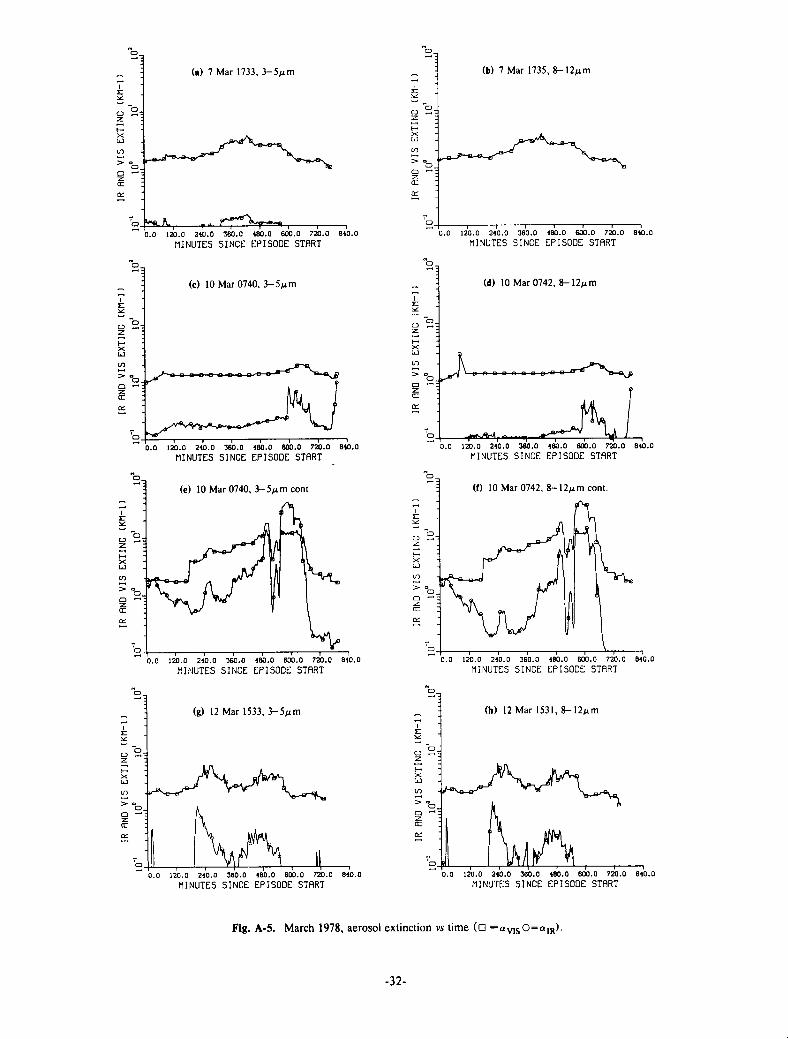
UJ

(n

o —

(a) 7 Mar 1733, 3-5/xm

0.0 120.0 240.0 360.0 480.0 600.0 720.0 840.0

MINUTES SINCE EPISODE START

(b) 7 Mar 1735, 8-12/xm

1 r—-—i 1 1 1 1 0.0 120.0 240.0 360.0 480.0 600.0 720.0 840.0

MINUTES SINCE EPISODE START

(c) 10 Mar 0740, 3-5/xm

„V~*~

120.0 240.0 360.0 480.0 600.0 720.0

MINUTES SINCE EPISODE START

(d) 10 Mar 0742, 8-12/xm

0.0 120.0 240.0 360.0 460.0 600.0 720.0 840.0 MINUTES SINCE EPISODE START

(e) 10 Mar 0740, 3-5/xm cont (f) 10 Mar 0742, 8-12/xm cont.

120.0 240.0 360.0 460.0 600.0 720.0 MINUTES SINCE EPISODE START

0.0 120.0 240.0 360.0 480.0 600.0 720.0 840.0

MINUTES SINCE EPISODE START

(g) 12 Mar 1533, 3-5/xm

120.0 240.0 360.0 480.0 600.0 720.0 MINUTES SINCE EPISODE START

(h) 12 Mar 1531, 8-12/xm

0.0 120.0 240.0 360.0 480.0 600.0 720.0 840.0

MINUTES SINCE EPISODE START

Fig. A-5. March 1978, aerosol extinction vs time ( o = a v i s ° = a i R ^

-32-

~ : (a) 21 Mar 0149, 3-5/xm

2% i— X UJ

R

AND

VIS

!0°

'o . ^^~^«^J^ 0.0 120.0 240.0 360.0 480.0 600.0 720.0 840.0

MINUTES SINCE EPISODE START

(c) 25 Mar 0011, 3-5/xm

— 3

- : (b) 21 Mar 0151, 8-12Mm i

sr

Z~°-. z t—

-J

Q -•*:

£ : a:

'o . -^-f o—1 1 1 1 1 1 0 0 120.0 240 0 360.0 480.0 600.0 720.0 840.0

MINUTES SINCE EPISODE START

(d) 25 Mar 0009, 8-12/xm

- I 1 " " I 1 1-

0.0 120.0 240.0 360.0 480.0 600.0 720.0 840.0 MINUTES SINCE EPISODE START

0 0 120.0 240.0 360.0 480.0 600.0 720.0 840.0 MINUTES SINCE EPISODE START

(e) 30 Mar 0140, 3-5/xm

1 1 1 1 1 1 1 0 0 120.0 240.0 360 0 480.0 600.0 720.0 940.0

MINUTES SINCE EPiSOJL STPRT

(f) 30Mar0138, 8-12Mm

o 2-=

-< LJ

CO

z

/ U V ^ V ^ ^ - ^ V A .

en

o ML., AAA\ 0.0 120.0 240.0 360.0 460.0 600.0 720.0 640.0

MINUTES SINCE EPISODE START

(g) 30 Mar 0140, 3-5/xm cont

MINUTES SINCE EPISODE START

(h) 30 Mar 0138, 8-12/xm cont

0 0 120 0 240 0 360 0 480 0 600 0 720 0 840 0

MINUTES SINCE EPISODE START

Fig. A-6. March 1978, aerosol extinction vs time ( • = a V I S 0 = a m )

-33-

(a) 5Sep2320, 3-5Mm

1 1—i i i i i 11 1 1—i—i I ' T i - q

10" 10' 102

VISIBLE EXTINCTION (KM-1)

(b) 5 Sep 2345, 8-12/xm

10° 10' 10" VISIBLE EXTINCTION (KM-1)

(c) 6 Sep 2110, 3-5/xm

° ft ft%™

at « _,rP°D

I T T | ^ 1 1 1—I 1 1 1 ]

10° 10' 10J

VISIBLE EXTINCTION IKM-1)

(d) 6 Sep 2112 8-12/xm

-%

• • B

o -. • D

D

% Doo,P o

" 1

%

D

D D a

1 1 1 1 1 - M |

10" 10" 10' VISIBLE EXTINCTION (KM-1)

(e) 7 Sep 1830, 3 - 5 M m

- D

• ° o

O O " D

1 » 9 i i i i i i | 1 i |

\ (f) 7 Sep 1836, 8-12Mm

; D

D o • a

a

: o o

1 i ° M i i n

ao o

1 1—i—rrTrn 10 10 10

VISIBLE EXTINCTION (KM-1) 10 10 10

VISIBLE EXTINCTION (KM"1)

(g) 9 Sep 0226, 3-5/xm

- ™ i — i — — i — i — 1 1 1 1 H I 10" 10 10

VISIBLE EXTINCTION (KM-1) '

(h) 9 Sep 0228, 8-12/xm

— ^ I — I — t r i i i ] r 1 — i — i I I I I )

10° 10' 10' VISIBLE EXTINCTION (KM-1)

Fig . A-7 . September 1978, infrared aerosol extinction vs visible extinction.

-34-

(a) 14 Sep 0858. 3-5/xm

10" 10' 101

VISIBLE EXTINCTION (KM-1)

(b) 14 Sep 0900, 8-12/xm

10" 10' 10' VISIBLE EXTINCTION (KM-1)

(c) 22 Sep 0234, 3 - 5 / x m

10" 10' 101

VISIBLE EXTINCTION (KM-1)

(d) 22 Sep 0228, 8-12/xm

T—i—i—i i i 11 1 1—i—i—i i i r |

10" 10' 10" VISIBLE EXTINCTION (KM-1)

(e) 22 Sep 1534, 3-5/xm

10" 10' 10' VISIBLE EXTINCTION (KM-1)

(f) 22 Sep 1616, 8-12/xm

'-,* 10' !0'

VISIBLE EXTINCTION (KM-i:

(g) 28 Sep 2334. 3-5/xm

'—r—T—I I I I | 1 1 1—1 I T T T 1

10" 10' 102

VISIBLE EXTINCTION (KM-1)

(h) 28 Sep 2332, 8 - 1 2 / x m

— i 1 — i i i i 1 1 1 i 1 — 1 1

10" 10' 10 ' VISIBLE EXTINCTION (KM-1)

Fig. A-8. September 1978, infrared aerosol extinction vs visible extinction

-35-

5"b UJ «• }f

1 T I I I I I I | 1 1 1 I I 1 I I |

10° 10' 101

VISIBLE EXTINCTION (KM-1)

— i — i — i i i i 1 1 1 1 1 — i — i i 1 1 1 1

10° 10' 102

VISIBLE EXTINCTION (KM-1)

(a) 3-5/xm (b) 8-12/xm

• = 6 Sep 0639 O = 10 Sep 0602 A = 13 Sep 0554 + = 13 Sep 1630 x = 13 Sep 2030

D = 6 Sep 0637 O =» 13 Sep 2036

o°o

-1 1—I—I I I I I I 10" 10' 102

VISIBLE EXTINCTION (KM-1)

+4 J* .

1 1 1—I' TT I I 1 r ~ 1 r T T T T T l 10" 10' 10a

VISIBLE EXTINCTION (KM-1)

(c) 3-5/xm (d) 8-12/xm

D = 17 Sep 0430 O = 30 Sep 2203

D = 17 Sep 0432 O = 22 Sep 1532 A = 27 Sep 0852 + = 30 Sep 2145

Fig. A-9. September 1978, infrared aerosol extinction vs visible extinction.

-36-

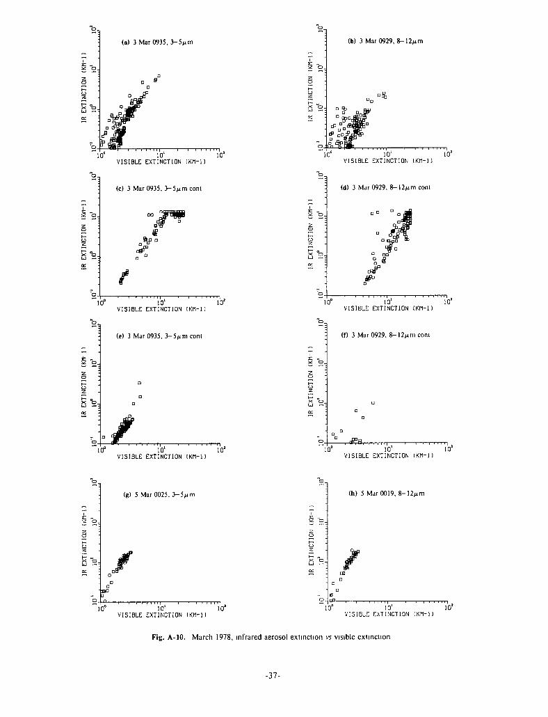
" (a) 3 Mar 0935, 3-5/xm

-a

. 0 «

' a

D

fl2 " Mf

&jF . a cf_jn

- Jr ? # , , T i t i 11 i 1—i—r-rr-rn

.-, -; (b) 3 Mar 0929, 8 - 1 2 M m

i 71 -\c o_ z: :

o

*-> z n ° * t— a

D D

x o_ D R)

CC ° f f D ; ^

I D

* r.uS'r " D fipfift

10° 10' 10' VISIBLE EXTINCTION (KM-1)

10 10 10' VISIBLE EXTINCTION (KM-1)

(c) 3 Mar 0935, 3-5/xm cont

>

1 f—-i—f r i - i T | 1 1—i—i i i T 11

10° 10' 101

VISIBLE EXTINCTION (KM-1)

— •3

'• (d) 3 Mar 0929, 8-12/xm cont

M 0 . °D °°M O'jjjfl

0 Aj«_> e— ° °£\ z f— 0 x 0 . a an CC '•

•flf a

'o_ 1 — —1—1—1 T T 1 n 1 1—1—r i - r r n

10" 10' 102

VISIBLE EXTINCTION (KM-1)

(e) 3 Mar 0935, 3-5/xm cont

1 1 — 1 — 1 — 1 1 1 1 1 1

10" 10' 102

VISIBLE EXTINCTION (KM-1)

(f) 3 Mar 0929, 8-12/xm com

- ^ S r T & T — r - i - r r r | 1 ' — • — ' • ' ' ' ' I 10° 10' 102

VISIBLE EXTINCTION (KM-1)

(g) 5 Mar 0025, 3-5/xm

—I 1—r-T~TTT| 1 1 1 — r _ T ' T ' l I 1

10" 10' 102

VISIBLE EXTINCTION (KM-1)

(h) 5 Mar 0019, 8-12/xm

10" 10' 102

VISIBLE EXTINCTION (KM-1)

Fig. A-10. March 1978, infrared aerosol extinction vs visible ext inct ion

-37-

(a) 7 Mar 1733, 3-5/xm

farJf ^ — i — i I I i I | 1 1—i—t—r

10° 10' VISIBLE EXTINCTION (KM-1)

10'

(b) 7 Mar 1735, 8-12Mm

—

EX

TIN

CTI

ON

10°

(all data offscale)

CC

'o_ 10° 10' 102

VISIBLE EXTINCTION (KM-1)

(c) 10 Mar 0740, 3-5/xm

o \

~ ' — i — i ' i i i 11 i i—r- i u r n 10" 10' 10'

VISIBLE EXTINCTION (KM-1)

(d) 10 Mar 0742, 8-12/xm

10° ~ ' ' i i 11 n 1 1—i—i—i i i r i

10' 102

VISIBLE EXTINCTION (KM-1)

(e) 0 Mar 0740, 3-5/xm cont

$»°m ;

q9

f r - jr - — — i — i — i 1 1 1 1 I I — i — i — 10" 10' 102

VISIBLE EXTINCTION (KM-1)

(f) 10 Mar 0742, 8-12/xm cont

oV

— ^ " — I — I I I I I M 1 1 — I I I 11]

10" 10' 102

VISIBLE EXTINCTION (KM-1)

(g) 12 Mar 1533, 3-5/xm

a u o

- » * l 10" 10' 102

VISIBLE EXTINCTION (KM-1)

(h) 12 Mar 1531, 8-12/xm

jB<3

ffl. 1 ' ' I , i i—'—r-T-rTT)

10" 10' 102

VISIBLE EXTINCTION (KM-1)

Fig. A - l l . March 1978, infrared aerosol extinction vs visible extinction.

-38-

(a) 21 Mar 0149, 3-5/xm

£Pg| - 1 — 1 — i — i 1 — i — i , i i i , |

10 10 10 VISIBLE EXTINCTION (KM-1)

(b) 21 Mar0151,8-12Mm

TIO

N

(KM

1

10'

o z X o LJ — :

CC '-

o . W&E)—,— 1—i—i , i i , , ) i0" 10' 102

VISIBLE EXTINCTION (KM-1)

(c) 25 Mar 0011, 3-5/xm

i , i 11 M 1 — i — i i i 11 M

10" 10 102

VISIBLE EXTINCTION (KM-1)

(d) 25 Mar 0009, 8-12/xm

10" 10' 102

VISIBLE EXTINCTION (KM-1)

(e) 30 Mar 0140, 3-5/xm

10" 10' 10J

VISIBLE EXTINCTION (KM-!)

(f) 30 Mar 0138, 8-12/xm

10 10 VISIBLE EXTINCTION (KM-1)

(g) 30 Mar 0140, 3-5/xm com

— i 1 — i , i i 1 1 1 1 1 — i — i i 1 1 n

10" 10' 10' VISIBLE EXTINCTION (KM-1)

(h) 30 Mar 0138, 8-12Mmcont

~ 2Z _

z '-o t— o z x: o LJ r- •

Srffitf - Wm _o

'o_ " 1 1 1 1—1 1 I I I 1 1 1 1—l~T~TT1

10 10 10 VISIBLE EXTINCTION (KM-1)

Fig. A-12. March 1978, infrared aerosol extinction vs visible extinction

-39-

- -i l ^ f a

10° T—i—i i r i1 r i i 1—i—i i r i T |

10' VISIBLE EXTINCTION (KM-1)

102

J ++ t ° : A

OH i — , — i i i i i | 1

10" 10' VISIBLE EXTINCTION (KM-1)

T—i—I r i 11

102

(a) 3-5/xm (b) 8-12/xm

Q = 3 Mar 0459 O = 3 Mar 0839 A = 4 Mar 2101 + = 5 Mar 0857 X = 7 Mar 1137

D = 3 Mar 0449 O = 3 Mar 0841 A = 4 Mar 2103 + = 5 Mar 0859

10" 10' VISIBLE EXTINCTION (KM-1)

10a o \m °, i i i i M , 1 1 — I ,

10° 10 10 VISIBLE EXTINCTION (KM-1)

(c) 3-5/xm (d) 8-12/xm

D = 7 Mar 1533 O = 8 Mar 1033 A = 10 Mar 0624 + = 12 Mar 1233 x = 13 Mar 2231

• = 9 Mar 1535 O = 12 Mar 1231 A = 13 Mar 2233 + = 13 Mar 2345

Fig. A-13. March 1978, infrared aerosol extinction vs visible extinction

-40-

—i—r- i -TTn ' — r i i i 1111 10" 10' 102

VISIBLE EXTINCTION (KM-1)

J 2-*r

10" 10' VISIBLE EXTINCTION (KM-1)

10'

(a) 3-5/xm

D = 14 Mar 0243 O - 19 Mar 1859 A = 19 Mar 2231 + = 22 Mar 0848 X = 22 Mar 2132

(b) 8-12/x m

a = 19 Mar 1857

o 19 Mar 2233 A 22 Mar 0846

+ D 22 Mar 2130

,-n— 10

VISIBLE EXTINCTION (KM-1) 102 10" 10'

VISIBLE EXTINCTION (KM-1) 10'

(c) 3-5/xm

D = 27 Mar 1515

o = 27 Mar 2347 A = 28 Mar 0559 + = 28 Mar 1504 X = 30 Mar 2136

(d) 8-12/xm

• = 27 Mar 1517 O = 27 Mar 2345 A = 28 Mar 0601 + = 28 Mar 1402 X = 28 Mar 1502 0 = 30 Mar 2134

Fig. A-14. March 1978, infrared aerosol extinction vs visible extinction

-41-

APPENDIX B

Plots of Prob

This appendix contains most of the probability plots which were generated for the analysis in Section 3. All of the types of probability estimates listed in Table 3.2 were computed and plotted. The resulting plots are included here except as follows.

Plots of P[aiRU+A)>T\av,sU)>l km"1 & RH(t)>80%] are not included because the results are nearly identical to plots of P[a/R(t+A) > T | Vis(t)> 1 km~n. The companion plots P[RH>T] and P[RH(t+A)>T \ RH(t)>T], which were used to

y Estimates

analyze the above, are also not included. Sample plots of these data are included in Fig. 3-8. Also, the plots of P[a/R (hr)> T \a/R (t = dawn)> T] are excluded since there were insufficient data to provide an accurate esti­mate. A sample plot is included in Fig. 3-9.

Following these plots are two flowcharts illustrating sample probability computations as discussed in Section 3.1. These flowcharts indicate the conceptual flow. The actual programs accomplished equivalent procedures in somewhat different order, for efficiency.

SYMBOLS D-HOUR-00 o "HOUR-02 a -HOUR-04 + -HOUR-20 X -HOUR-22

I

0 . 2 0 . 1 0 .6 0 . 6 1.0 1.2 1.1

THRESHOLD EXTINCTION (KM-1)

(a) Sep '78 3-5/xm, Prob vs Thresh

SYMBOLS o -HOUR-00 o -HOUR-02 A -HOUR-Oi + -HOUR-20 X -HOUR-22

0.2 0.4 0.6 0.8 1.0 1.2

THRESHOLD EXTINCTION (KM-1)

(b) Sep '78 8-12/xm, Prob vs Thresh

SYMBOLS • -HOUR-00 o -HOUR-02 A -HOUR-Oi + -HOUR-20 X -HOUR-22

0 . 2 0 .4 0 . 6 0 . 6 1.0 1.2

THRESHOLD EXTINCTION (KM-1)

-" CC

a X

21 CJ

a: LJ

a ~

d~

\ SYMBOLS \ \ • "HOUR-00 \ f l o - H O U R - 0 2 W A -HOUR-04 1 \ + -HOUR-20 1 \ X -HOUR-22

>- ,

CD

a: CD O CC Q_

CM

d"

o d •» — ft

CM

d"

o d

I 1 1 T -f — 9 = T - = a — 1 0.0 0.2 0.4 0.6 0.8 1.0 1.2 1.4

THRESHOLD EXTINCTION (KM-1)

(c) Mar '78 3-5/xm, Prob. vs Thresh (d) Mar'78 8-12/xm, Prob vs Thresh

oo o »• 9= d

SYMBOLS • - T-0.7 o - T-0.9 « - T-1.0 + - T-1.1 X - T-1.3 • - T-1.5

***w - i r-0 . 0 2 . 0 4 . 0 6 . 0 8 . 0 10 .0 12 .0 14 .0 16 .0 18 .0 2 0 . 0 2 2 . 0 2 4 . 0

HOUR

(e) Sep '78 3-5/xm, Prob vs Hour

SYMBOLS o - T-0.3 O - T-0.S A - T-o.a * - T-1.0 X - T-1.2 0 - T-l 5

•45*4affi^-0 . 0 2 . 0 4 .0 6 . 0 8 . 0 10 .0 12.0 14 .0 16 .0 18.0 2 0 . 0 2 2 . 0 24 .0

HOUR

(f) Sep '78 8-12/xm, Prob vs Hour

SYMBOLS D - T-0.7 o - T-0.9 a - T-1.0 + - T-1.1 X - T-1.3 o - T-1.5

~l 1 0.0 2.0 4.0

+ • + • ? • ? • i.O 6 . 0 10.0 12 .0 14 .0 16 .0 18 .0 2 0 . 0 2 2 . 0 24 .0

HOUR

SYMBOLS • - T-0.3 o - T-0.5 4 - T-0.8 + - T-1.0 X - T-1.2 o - T-1.5

(g) Mar '78 3-5/xm, Prob vs Hour

0.0 2.0 4.0 6.0 8.0 10.0 12.0 14.0 16.0 18.0 20.0 22.0 24.0 HOUR

(h) Mar '78 8-12/xm, Prob vs Hour

Fig. B - l . Night Probability vs Hour /> = P[a,R (hr) > T ]

-43-

SYMEOLS • - pi o - P2UJW 16) « - P2ime 60) + - P21LH6 1BO) X - P21LIW 3601

0 2 0 4 0 6 0 8 1 0 1 2 1 1

THRESHOLD EXTINCTION (KM-1)

(a) Sep '78 3-5>im, Prob vs Thresh

0 4 0 6 0.8 10

THRESHOLD EXTINCTION

SYMBOLS P2[U» 16) P2ILAS 60) P2ILA6 ISO) P2ILH0 360)

1 2

(KM-1)

(b) Sep '78 8 -12^m, Prob vs Thresh

>~ ^ SYMBOLS

02 04 06 06 10 12 14 THRESHOLD EXTINCTION (KM-1)

(c) Mar'78 3 -5 / im, Prob vs Thresh

0 2 0 4 0 6 0 8 1 0 1 2 I

THRESHOLD EXTINCTION (KM-1)

(d) Mar '78 8-12/* m, Prob vs Thresh

_ *$5fc«v

SYMBOLS " ^ = = = = — * • "» T-0 7 o - T-0 9 A - T-l 0 + - T-l 1 X " T-l 3 o - T-l 5

60 0 120 0 180 0 240 0 300 0

LAG IN MINUTES

(e) Sep '78 3—5^m, Pers vs Lag

120 0 180 0 240 0

LAG IN MINUTES 300 0 360 0

(f) Sep'78 8-12(um Pers vs Lag

120 0 160 0 240 0 300 0 360 0

LAG IN MINUTES 120 0 180 0 240 0 300 0 360 0

LAG IN MINUTES

(g) Mar '78 3 -5 / im, Pers vs Lag (h) Mar '78 8-12/xm, Pers vs Lag

Fig. B-2 . Night Probabilities PI = P[aIR > T ] , P2 = P[a,R (H-A) >T\a,R(t)>T)

-44-

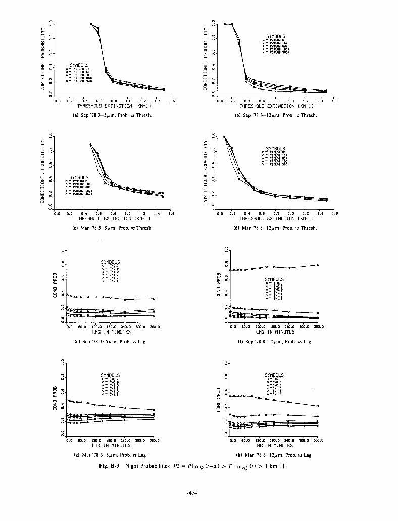
SYMBOLS o - P2[Lfltf O) O - P2IUW 16) 4 - P2US 601 + - P2ILA8 160) X - P2ILA8 360)

0 . 2 0 .4 0 . 6 O.B 1.0 1.2 1.4

THRESHOLD EXTINCTION (KM-1)

(a) Sep '78 3-5Mm, Prob. vs Thresh.

SYMBOLS n - P2IUW 01 o - P2IUW 16) a - P2IUW 60) + - P2IUW ISO) X - P2IUS 360)

.2 0.4 0.6 0.6 1.0 1.2 1.4

THRESHOLD EXTINCTION (KM-1)

(b) Sep '78 8-12/nm, Prob. vs Thresh.

SYMBOLS n - P2ILR8 0) o - P2ILAC 16) A - P2ilflB 60) + - P2(Lflfl 1B0) X - P2ILA8 360)

0 . 2 0 .4 0 . 6 0 .6 1.0 1.2 1.4

THRESHOLD EXTINCTION (KM-1)

(c) Mar '78 3— 5j im, Prob. vs Thresh.

SYMBOLS D - P2ILA8 0) o - P2IUW 16) 4 - P2ILA8 60) + - P2CUW 160) X - P2IUIB 360)

0 . 2 0 . 4 0 . 6 0 . 8 1.0 1.2 1.4

THRESHOLD EXTINCTION (KM-1)

(d) Mar '78 8-12/um, Prob. vs Thresh.

SYMBOLS a- T-0.7 o - 1-0.9 « - T-1.0 + - I - I . l X - T- l .3 0 - T-I.S

-

" SYMBOLS a- 1-0.3 o - r-o.s 4 - I-O.B • » - r - i .o X - 1-1.2 • - r-i.s

; ^ ^ ^ ; ^ ^ ^ 1 i i

6 0 . 0 120.0 180.0 240 .0 300 .0 360 .0

LUG IN MINUTES

(e) Sep '78 3— 5/iin, Prob. vs Lag

l 60.0 120.0 180.0 240.0 300.0 360.0

LAG IN MINUTES

(f) Sep '78 8-12/tm, Prob. vs Lag

) 60.0 120.0 180.0 240.0 300.0 360.0

LAG IN MINUTES

(g) Mar '78 3-5 / im, Prob. vs Lag

Fig. B-3. Night Probabilities P2

0.0 60.0 120.0 180.0 240.0 300.0 360.0

LAG IN MINUTES

(h) Mar '78 8-12)nm, Prob. vs Lag

P[a,R(t+b)>T \am(t)> 1 k m - ' ] .

-45-

SYMBOLS D - P2ILP.B 0) o - P21LAC 16) A - P21LP.G 60) + - P21LP.G 160)

2 04 06 08 10 12 1 THRESHOLD EXTINCTION (KM-1)

(a) Sep '78 3-5 / im, Prob vs Thresh

2 04 06 08 10 12 1 THRESHOLD EXTINCTION (KM-1)

(b) Sep '78 8-12^m, Prob vs Thresh

" 1 > H

r—

1 CD

\ \ m \ (T \ rn \ o \ i

a. O

• * * SYMBOLS a. O

O " O - P21LAC 0) a. O 0 - P2ILAB 16)

A - P2ILAC 60) rvj + - P21LAC 160)

n X n o o

o . 0 2 0 4 0 6 0 8 1 0 1 2 1 4

THRESHOLD EXTINCTION (KM-1)

(c) Mar '78 3-5/im, Prob vs Thresh

SYMBOLS D - P2ILP.8 0) o - P2ILAG 16) A - P2ILA8 60) + - P2ILAB 160) X - P21Ufl8 360)

0 4 0 6 0 8 1 0

THRESHOLD EXTINCTION 1 2 1 4

(KM-1)

(d) Mar'78 8-12Mm Prob vs Thresh

60 0 120 0 180 0 240 0 300 0 360 0

LAG IN MINUTES

(e) Sep '78 3-5 / im, Prob vs Lag

~[^™^7C SYMBOLS \ \ • - T-0 3 \ • o - T-0 5 \ • - H I \

120 0 180 0 240 0 LAG IN MINUTES

300 0 360 0

(f) Sep '78 8-12/ixm, Prob vs Lag

SYMBOLS D - T-0 7 o - T-0 9 4 - T-l 0 + - T-l 1 X - T-l 3 » - T-l 5

120 0 180 0 240 0 LAG IN MINUTES

300 0 360 0 120 0 180 0 240 0

LAG IN MINUTES 300 0 360 0

(g) Mar '78 3-5/i.m, Prob vs Lag

Fig. B-4. Night Probabilities P2

(h) Mar'78 8-12/im Prob vs Lag

P[aIR(t+A) > T \avls(t) > 4 k m - ' ]

-46-

E=fe£

SYMBOLS 3 - PI 3 - P2IL6C 16) i - P2ILP.8 60) • - P2ILHS 160) < - P2H.P.S 360)

0 4 0 6 0 8 1 0

THRESHOLD EXTINCTION 1 2

(KM-1)

(a) Sep 78 Night, Prob vs Thresh

SYMBOLS

0 4 0 6 0 8 10

THRESHOLD EXTINCTION 1 2 1

(KM-1)

(b) Mar '78 Night Prob vs Thresh

SYMBOLS T-0 7 T-0 9 T-l 0 T-l 1

60 0 120 0 180 0 240 0 300 0

LAG IN MINUTES

(c) Sep '78 Night, Pers vs Lag

120 0 ISO 0 240 0

LAG IN MINUTES 300 0 360 0

(d) Mar '78 Night, Pers vs Lag

SYMBOLS D - PI o - P2ILAB 16) » - P2ILH8 60) + - P21LA8 1B0) X - P2(me 360)

0 4 0 6 0 6 1 0 1 2

THRESHOLD EXTINCTION (KM-1)

(e) Sep '78 Day Prob vs Thresh

o — o — © — o — e — o — e — e — * •

SYMBOLS • - pi o - P21LA8 16) 4 - P2ILA8 60) + - P21LAB 160) X - P2CLAB 360)

0 4 0 6 0 8 1 0

THRESHOLD EXTINCTION 1 2

(KM-1)

(f) Mar 78 Day Prob vs Thresh

^^

SYMBOLS V ^ C ^ ^ N ^ o - T-0 7 \ w ^ * - - ^ ^ o - T-o 9 ^fcr—-__^ ^ ^ ^ - t A • T-l 0 ^ ^ J ^ ^ ^ - - ^ ^ + ~ T-l 1 ^ ^ S J L ^ " " - - • • ^ x - T-l 3 ^ ^ ^ s : ^ ^ ^ " " - - . f o - T-l 5 ^^"^^^s^x

120 0 160 0 240 0

LAG IN MINUTES 300 0 360 0

(g) Sep '78 Day Pers vs Lag

120 0 160 0 240 0 LAG IN MINUTES

300 0 360 0

(h) Mar '78 Day, Pers vs Lag

Fig. B-S. Night & Day Probabilities PI = P[avls > T ] , P2 = Plamb+A) > T \amd) > T 1

-47-

SYMBOLS HOUR-06 HOUR-09 HOUR-12 HOUR-15 HOUR-18

1 SYMBOLS 4J D - HOUR-06 1 0 - HOUR-09 1 4 - HOUR-12 1 • - HOUR-IS 1 X - HOUR-16

02 04 06 08 10 12 14 THRESHOLD EXTINCTION (KM-1)

(a) Sep'78 3 -5 / im Prob vs Thresh

02 04 06 08 10 12 14 THRESHOLD EXTINCTION (KM-1)

(b) Sep '78 8-12/xm, Prob vs Thresh

SYMBOLS • - HOUR-06 o - HOUR-09 4 - HOUR-12 * - HOUR-15 X - HOUR-18

SYMBOLS O - HOUR-06 O - HOUR-09 4 - HOUR-12 • - HOUR-15 X - HOUR-16

- I -0 2 0 4 0 6 0 8 1 0 1 2 1 4

THRESHOLD EXTINCTION (KM-1) 0 2 0 4 0 6 0 8 1 0 1 2 1 4

THRESHOLD EXTINCTION (KM-1)

(c) Mar '78 3 -5 / im, Prob vs Thresh (d) Mar '78 8-12/ im, Prob vs Thresh

SYMBOLS D - T-0 7 0 - T-0 9 A ~ T-l 0 + ~ T-l 1 x -0 -

T-l 3 T-l 5

- 1 i r ID O <D SYM 31 ° D -

0 -T r t (T

0 — LJ O " 0 —

>-f—

_) Q-m u CD fM

<r Q_

O

°-O

°-

T-0 3 T-0 5 T-0 6

0 0 2 0 4 0 6 0 8 0 10 0 12 0 14 0 16 0 16 0 20 0 22 0 24 0

HOUR

(e) Sep '78 3-5/xm, Prob vs Hour

0 0 2 0 4 0 6 0 8 0 10 0 12 0 14 0 16 0 18 0 20 0 22 0 24 0

HOUR

(f) Sep '78 8-12/ im, Prob vs Hour

SYMBOLS n - T-0 7 o - T-0 9 4 - T-l 0 * - T-l 1 X - T-l 3 » - T-l 5

SYMBOLS o - T-0 3 o - T-0 5 4 - T-0 B + - T-l 0 X - T-l 2 9 - T-l 5

0 0 2 0 4 0 6 0 8 0 10 0 12 0 14 0 16 0 18 0 20 0 22 0 24 0

HOUR

(g) Mar '78 3 -5 / im, Prob vs Hour

0 0 2 0 4 0 6 0 6 0 10 0 12 0 14 0 16 0 IB 0 20 0 22 0 24 0

HOUR

(h) Mar '78 8-12/ im, Prob vs Hour

Fig. B-6. Day Probability vs Hour P = P[am (hr) > T ]

-48-

SYMBOLS

o - P2ll.R0 16) 4 - P2ILRG 60) + - P2ILP.S 180) X - P2ILPB 360)

SYMBOLS

0 2 0 4 0 6 0 8 1 0 1 2 1 4

THRESHOLD EXTINCTION (KM-1)

(a) Sep '78 3-5^111, Prob vs Thresh

0 2 0 4 0 6 0 8 1 0 1 2 1 4

THRESHOLD EXTINCTION (KM-1)

(b) Sep '78 8 - 1 2 M m , Prob vs Thresh

SYMBOLS a - pi o - P2IIR8 16) 4 - P2H.RB 60) + - P2ILR6 1BO) X - P2ILP.G 360)

SYMBOLS

o - P2(LP.G 16) 4 - P2ILP.B 60) + - P2II.P.G 160) X - P21LP.C 360)

0 4 0 6 O B 1 0

THRESHOLD EXTINCTION 1 2 1 4

(KM-1)

(c) Mar '78 3-5/im, Prob vs Thresh

02 04 06 OB 10 12 14

THRESHOLD EXTINCTION (KM-1)

(d) Mar '78 8-12/im, Prob vs Thresh

SYMBOLS a - T-0 7 o - T-0 9 4 - T-l 0 + - T-] 1

120 0 180 0 240 0

LAG IN MINUTES 300 0 360 0

(e) Sep '78 3-5/im, Pers vs Lag

60 0 120 0 160 0 240 0 300 0 360 0

LAG IN MINUTES

(f) Sep '78 8 - 1 2 / i m , Pers vs Lag

SYMBOLS

0 0 60 0 ' 20 0 180 0 240 0 300 0 360

LAG IN MINUTES

SYMBOLS a - T-0 3 O - T-0 5 4 - T-0 8 t - 1-1 0 X - T-l 2 » - W S

120 0 ISO 0 240 0

LAG IN MINUTES 300 0 360 0

(g) Mar '78 3-5/im, Pers vs Lag (h) Mar '78 8-12ju.m, Pers vs Lag

Fig. B-7. Day Probabilities PI = Pi a,R > T] , P2 = P[ a,R ( /+A)> T | aIR (r) > 7"]

-49-

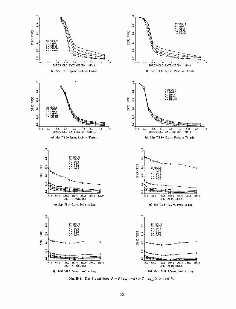
SYMBOLS LP.G-0 LPrS-16 LRB-60 LRB-160 LRC-360

0.2 0.4 0.6 0.8 1.0 1.2 1.4

THRESHOLD EXTINCTION (KM-1)

(a) Sep '78 3-5/xm, Prob. vs Thresh.

0 . 2 0 .4 0 .6 0 . 6 1.0 1.2 1.4

THRESHOLD EXTINCTION (KM-1)

(b) Sep '78 8-12/ im, Prob. vs Thresh.

SYMBOLS D - LRO-0 o - LR8-16 4 - me-60 + - Lflo-ieo X - LflB-360

0 . 2 0 . 4 0 . 6 0 . 8 1.0 1.2 1.4

THRESHOLD EXTINCTION (KM-1)

(c) Mar '78 3 -5 / im, Prob. vs Thresh.

0 . 2 0 . 4 0 . 6 0 . 6 1.0 1.2 1.4

THRESHOLD EXTINCTION (KM-1)

(d) Mar '78 8-12/ im, Prob. vs Thresh.

120.0 180.0 240 .0

LAG IN MINUTES 300.0 360.0

(e) Sep '78 3-5/1"!, Prob. vs Lag

0 . 0 6 0 . 0 120.0 1B0.0 240 .0 300 .0

LAG IN MINUTES

(f) Sep '78 8-12/ im, Prob. vs Lag

SYMBOLS SYMBOLS • - T-0.3 o - T-0.5 4 - T-0.8 + - T-1.0 X - T-l .2 • - T-l .5

0 . 0 6 0 . 0 120.0 180.0 240 .0 300 .0 360 .0

LAG IN MINUTES

(g) Mar '78 3-5/xm, Prob. vs Lag

Fig . B-8. Day Probabilities P ••

0 .0 6 0 . 0 120.0 180.0 240 .0 300 .0 3 6 0 . 0

LAG IN MINUTES

(h) Mar '78 8-12/im, Prob. vs Lag

P[am(t+A) > T | a r a ( f ) > l k m - ' ] .

-50-

SYMBOLS a - LfiO-0 O - LB8-16 4 - LRS-tO + - LR8-160

LflO-360

0 2 0 4 0 6 0 6 1 0 1 2 1 4

THRESHOLD EXTINCTION IKM-1)

(a) Sep'78 3 -5 / im Prob vs Thresh

0 2 0 4 0 6 0 8 1 0 1 2 1 4

THRESHOLD EXTINCTION (KM-1)

(b) Sep'78 8-12/ im Prob vs Thresh

Q 2 O

CD O

SYMBOLS D - UW-0 o - LH8-16 4 - LflS-60 + - Lfts-ieo X - LR8- 360

0 2 0 4 0 6 0 8 1 0 1 2 1 4

THRESHOLD EXTINCTION (KM-1)

(c) Mar '78 3-5/xm, Prob vs Thresh

0 0 0 2 0 4 0 6 0 8 1 0 1 2 1 4

THRESHOLD EXTINCTION (KM-1)

(d) Mar'78 8-12/im Prob vs Thresh

o z o

SYMBOLS T-0 7 T-0 9 T-l 0 T-l 1 T-l 3 T-l S

60 0 120 0 180 0 240 0 300 0 360 0

LAG IN MINUTES

(e) Sep '78 3 -5 / im Prob vs Lag

0 0 60 0 120 0 IB0 0 240 0 300 0 360 0

LAG IN MINUTES

(f) Sep '78 8-12/ im, Prob vs Lag

SYMBOLS

I 60 0 120 0 180 0 240 0 300 0 360 0

LAG IN MINUTES

(g) Mar '78 3-5/xm, Prob vs Lag

Fig. B-9. Day Probabilities P •

0 0 60 0 120 0 160 0 240 0 300 0 360 0

LAG IN MINUTES

'h) Mar '78 8-12/xm, Prob vs Lag

PlalR(i+A)>T | a r a ( f ) > 2 k r r r ' ]

-51-

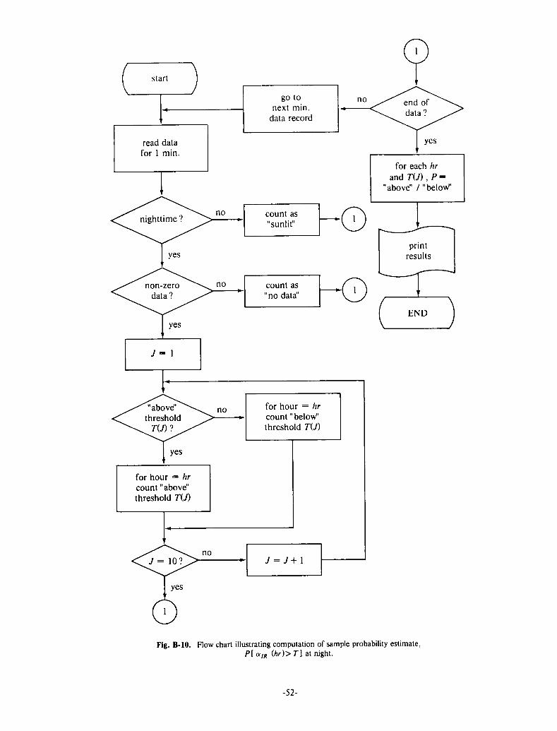
start

read data for 1 min.

for hour = hr count "above" threshold T(J)

go to next min.

data record

count as "sunlit"

count as "no data"

for hour = hr count "below" threshold TU)

J = J+l

for each hr and T(J),P =

"above" / "below"

print results

END

Fig. B-10. Flow chart illustrating computation of sample probability estimate, P[am (hr)>T] at night.

-52-

subchart

7 = 1

yes

for 7V), count as above" or" lag-above"

for lag K

count as "sunlit" or as "lag-sunlit"

for lag K -o count as "no data"

or "lag-no data" for lag K -o

for TU), count as "below" or "lag-below"

for lag K

yes

J = J+l

Start

read first 6 hours of

data

apply sub-chart i I to I first minute '

J

move 6 hour interval down

l record (4 mm)

1

K = l

' ~l 1 1 1

no

apply sub-chart to

min at lag A( K )

~l 1 1 1

no

I no

K = l C no

K = l C

yes

for each TU) PI =

"above" / "below"

for each TU) and lag, P2 -

"lag-abovd' "lag-belov)'

for each TU) and lag, r =

1 - P2 1 -

1 - PI

print results

end

Fig. B-ll. Flow chart illustrating computation of sample probability estimate, P[a U+&)> T | a (r)> T]

APPENDIX C

VISIBILITY LABORATORY CONTRACTS AND RELATED PUBLICATIONS

Previous Related Contracts: F19628-73-C-0013, F19628-76-C-0004

PUBLICATIONS:

Duntley, S.Q., R.W. Johnson, J.I. Gordon, and A. R. Boileau, "Airborne Measurements of Optical Atmospheric Properties at Night", University of Cali­fornia, San Diego, Scripps Institution of Oceanogra­phy, Visibility Laboratory, SIO Ref. 70-7, AFCRL-70-0137, NTIS No. AD 870 734 (1970).

Duntley, S.Q., R.W. Johnson, and J.I. Gordon, "Airborne Measurements of Optical Atmospheric Properties in Southern Germany", University of California, San Diego, Scripps Institution of Oceanography, Visibility Laboratory, SIO Ref. 72-64, AFCRL-72-0255, NTIS No. AD 747 490 (1972a).

Duntley, S.Q., R.W. Johnson, and J.I. Gordon, "Airborne and Ground-Based Measurements of Optical Atmos­pheric Properties in Central New Mexico", University of California, San Diego, Scripps Institution of Oceanography, Visibility Laboratory, SIO Ref. 72-71, AFCRL-72-0461, NTIS No. AD 751 936 (1972b).

Duntley, S.Q., R.W. Johnson, and J.I. Gordon, "Airborne Measurements of Optical Atmospheric Properties, Summary and Review", University of California, San Diego, Scripps Institution of Oceanography, Visibility Laboratory, SIO Ref. 72-82, AFCRL-72-0593, NTIS No. AD 754 898 (1972c).

Duntley, S.Q., R.W. Johnson, and J.I. Gordon, "Airborne Measurements of Optical Atmospheric Properties in Southern Illinois", University of California, San Diego, Scripps Institution of Oceanography, Visibility Laboratory, SIO Ref. 73-24, AFCRL-TR-73-0422, NTIS No. AD 774 597 (1973).

Duntley, S.Q., R.W. Johnson, and J.I. Gordon, "Airborne and Ground-Based Measurements of Optical Atmos­pheric Properties in Southern Illinois", University of California, San Diego, Scripps Institution of Oceanography, Visibility Laboratory, SIO Ref. 74-25, AFCRL-TR-74-0298, NTIS No. ADA 013 164 (1974).

Duntley, S.Q., R.W. Johnson, and J.I. Gordon, "Airborne Measurements of Optical Atmospheric Properties in Western Washington", University of California, San Diego, Scripps Institution of Oceanography, Visibility Laboratory, SIO Ref. 75-24, AFCRL-TR-75-0414, NTIS No. ADA 026 036 (1975a).

Duntley, S.Q., R.W. Johnson, and J.I. Gordon, "Airborne Measurements of Optical Atmospheric Properties, Summary and Review If, University of California, San Diego, Scripps Institution of Oceanography, Visibility Laboratory, SIO Ref. 75-26, AFCRL-TR-75-0457, NTIS No. ADA 022 675 (1975b).

Duntley, S.Q., R.W. Johnson, and J.I. Gordon, "Airborne Measurements of Optical Atmospheric Properties in Northern Germany", University of California, San Diego, Scripps Institution of Oceanography, Visibility Laboratory, SIO Ref. 76-17, AFGL-TR-76-0188, NTIS No. ADA 035 571 (1976).

Duntley, S.Q., R.W. Johnson, and J.I. Gordon, "Airborne Measurements of Atmospheric Volume Scattering Coefficients in Northern Europe, Spring 1976", University of California, San Diego, Scripps Institu­tion of Oceanography, Visibility Laboratory, SIO Ref. 77-8, AFGL-TR-77-0078, NTIS No. ADA 046 290 (1977).

Duntley, S.Q., R.W. Johnson, and J.I. Gordon, "Airborne Measurements of Atmospheric Volume Scattering Coefficients in Northern Europe, Fall 1976", Univer­sity of California, San Diego, Scripps Institution of Oceanography, Visibility Laboratory, SIO Ref. 78-3, AFGL-TR-77-0239, NTIS No. ADA 057 144 (1978a).

Duntley, S.Q., R.W. Johnson, and J.I. Gordon, "Airborne Measurements of Atmospheric Volume Scattering Coefficients in Northern Europe, Summer 1977', University of California, San Diego, Scripps Institu­tion of Oceanography, Visibility Laboratory, SIO Ref. 78-28, AFGL-TR-78-0168, NTIS No. ADA 068 611 (1978b).

Duntley, S.Q., R.W. Johnson, and J.I. Gordon, "Airborne Measurements of Optical Atmospheric Properties, Summary and Review III", University of California, San Diego, Scripps Institution of Oceanography, Visibility Laboratory, SIO Ref. 79-5, AFGL-TR-78-0286, NTIS No. ADA 073 121 (1978c).

Fitch, B.W. and T.S. Cress, "Measurements of Aerosol Size Distribution in the Lower Troposphere over Northern Europe", J. Appl. Met. 20, No. 10, 1119-1128, also University of California, San Diego, Scripps Institution of Oceanography, Visibility Laboratory, SIO Ref. 81-18, AFGL-TR-80-0192, NTIS No. ADA 104 272 (1981).

Gordon, J.I., C. F. Edgerton, and S.Q. Duntley, "Signal-Light Nomogram", J. Opt. Soc. Am. 65, 111-118 (1975).

Gordon, J.I., J. L. Harris, Sr., and S.Q. Duntley, "Measur­ing Earth-to-Space Contrast Transmittance from Ground Stations", Appl. Opt. 12, 1317-1324 (1973).

Gordon, J.I., "Model for a Clear Atmosphere", J. Opt. Soc. Am. 59, 14-18 (1969).

Gordon, J.I., "Daytime Visibility, A Conceptual Review", University of California, San Diego, Scripps Institu­tion of Oceanography, Visibility Laboratory, SIO Ref. 80-1, AFGL-TR-79-0257, NTIS No. ADA 085 451 (1979).

Gordon, J.I., "Implications of the Equation of Transfer Within the Visible and Infrared Spectrum", Univer­sity of California, San Diego, Scripps Institution of Oceanography, Visibility Laboratory, SIO Ref. 83-10, AFGL-TR-82-0223 (1983).

Hering, W. S., "An Operational Technique for Estimating Visible Spectrum Contrast Transmittance", Univer-

-54-

sity of California, San Diego, Scripps Institution of Oceanography, Visibility Laboratory, SIO Ref. 82-1, AFGL-TR-81-0198 (1981a).

Hering, W.S., "Assessment of Operational Techniques for Estimating Visible Spectrum Contrast Transmit­tance", SPIE Proceedings on Atmospheric Effects on System Performance, 205, 119-125 (1981b).

Johnson, R.W., W. S. Hering, J.I. Gordon, B. W. Fitch, and J.S. Shields, "Preliminary Analysis & Modelling Based Upon Project OPAQUE Profile and Surface Data", University of California, San Diego, Scripps Institution of Oceanography, Visibility Laboratory, SIO Ref. 80-5, AFGL-TR-79-0285, NTIS ADB 052 172L (1979).

Johnson, R.W. and B.W. Fitch, "A Review of Measured Atmospheric Optical Properties and Their Contem­porary Aerosol Size Distributions", University of California, San Diego, Scripps Institution of Oceanography, Visibility Laboratory, SIO Ref. 82-22, AFGL-TR-82-0049 (1981).

Johnson, R.W., and J.I. Gordon, "Airborne Measurements of Atmospheric Volume Scattering Coefficients in Northern Europe, Winter 1978", University of Cali­fornia, San Diego, Scripps Institution of Oceanogra­phy, Visibility Laboratory, SIO Ref. 79-25, AFGL-TR-79-0159, NTIS No. ADA 082 044 (1979).

Johnson, R.W. and J.I. Gordon, "Airborne Measurements of Atmospheric Volume Scattering Coefficients in Northern Europe, Summer 1978", University of Cali­fornia, San Diego, Scripps Institution of Oceanogra­phy, Visibility Laboratory, SIO Ref. 80-20, AFGL-TR-80-0207, NTIS No. ADA 097 134 (1980).

Johnson, R.W. and J.I. Gordon, "A Review of Optical Data Analysis Related to the Modelling of Visible and Optical Infrared Atmospheric Properties", University of California, San Diego, Scripps Institu­tion of Oceanography, Visibility Laboratory, SIO Ref. 83-5, AFGL-TR-82-0086 (1981).

Johnson, R.W. and W.S. Hering, "Measurements of Opti­cal Atmospheric Quantities in Europe and Their Application to Modelling Visible Spectrum Contrast Transmittance", AGARD Proceedings on Special Topics in Optical Propagation, AGARD-CP-300, pp. 14-1 to 14-12 (1981a).

Johnson, R.W. and W. S. Hering, "An Analysis of Natural Variations in Measured European Sky and Terrain

Radiances", University of California, San Diego, Scripps Institution of Oceanography, Visibility Laboratory, SIO Ref. 82-6, AFGL-TR-81-0317 (1981b).

Johnson, R.W., "Airborne Measurements of European Atmospheric Scattering Coefficients", SPIE Proceed­ings on Atmospheric Effects on Radiative Transfer, 195, 31-38 (1979).

Johnson, R.W., "Winter and Summer Measurements of European Very Low Altitude Volume Scattering Coefficients," University of California, San Diego, Scripps Institution of Oceanography, SIO Ref. 81-26, AFGL-TR-81-0154, NTIS No. ADA 106 363 (1981a).

Johnson, R.W., "Spring and Fall Measurements of Euro­pean Very Low Altitude Volume Scattering Coefficients", University of California, San Diego, Scripps Institution of Oceanography, Visibility Laboratory, SIO Ref. 81-33, AFGL-TR-81-0237, NTIS No. ADA 108 879 (1981b).

Johnson, R.W., "Daytime Visibility and Nephelometer Measurements Related to its Determination", Atmospheric Environment, 15, 10/11, 1835 (1981c).

Johnson, R.W., "Airborne Measurements of European Sky and Terrain Radiances", University of California, San Diego, Scripps Institution of Oceanography, Visibility Laboratory, SIO Ref. 82-2, AFGL-TR-81-0275 (1981d).

Johnson, R.W., "An Experimental Device for Real Time Determination of Slant Path Atmospheric Contrast Transmittance", University of California, San Diego, Scripps Institution of Oceanography, Visibility Laboratory, SIO Ref. 82-27, AFGL-TR-82-0125 (1982).

Johnson, R.W., "An Experimental Device for Real Time Determination of Slant Path Atmospheric Contrast Transmittance (Prototype Status)", University of Cal­ifornia, San Diego, Scripps Institution of Oceanogra­phy, Visibility Laboratory, SIO Ref. 83-14, AFGL-TR-83-0053 (1983).

Shields, J.S., "An Analysis of Infrared and Visible Atmos­pheric Extinction Coefficient Measurements in Europe", University of California, San Diego, Scripps Institution of Oceanography, Visibility Laboratory, SIO Ref. 82-4, AFGL-TR-81-0251 (1981).

-55-

Notes

-56-

Notes

-57-

Notes

-58-