sdr radar demonstrator using ofdm-modulation
TRANSCRIPT
Institutionen för systemteknikDepartment of Electrical Engineering
Examensarbete
SDR radar demonstrator using OFDM-modulation
Examensarbete utfört i Elektroniksystemvid Tekniska högskolan i Linköping
av
Jimmy KarlssonOskar Larsson
LiTH-ISY-EX--09/4266--SE
Linköping 2009
Department of Electrical Engineering Linköpings tekniska högskolaLinköpings universitet Linköpings universitetSE-581 83 Linköping, Sweden 581 83 Linköping


SDR radar demonstrator using OFDM-modulation
Examensarbete utfört i Elektroniksystemvid Tekniska högskolan i Linköping
av
Jimmy KarlssonOskar Larsson
LiTH-ISY-EX--09/4266--SE
Handledare: Lars-Ove LarssonEmerson Process Management
Fabian WengerEmerson Process Management
Examinator: Håkan Johanssonisy, Linköpings universitet
Linköping, 25 September, 2009


Avdelning, InstitutionDivision, Department
Division of Electronics SystemsDepartment of Electrical EngineeringLinköpings universitetSE-581 83 Linköping, Sweden
DatumDate
2009-09-25
SpråkLanguage
� Svenska/Swedish� Engelska/English
�
�
RapporttypReport category
� Licentiatavhandling� Examensarbete� C-uppsats� D-uppsats� Övrig rapport�
�
URL för elektronisk versionhttp://www.es.isy.liu.se
http://urn.kb.se/resolve?urn=urn:nbn:se:liu:diva-21094
ISBN—
ISRNLiTH-ISY-EX--09/4266--SE
Serietitel och serienummerTitle of series, numbering
ISSN—
TitelTitle
SDR radardemonstrator med OFDM-modulationSDR radar demonstrator using OFDM-modulation
FörfattareAuthor
Jimmy KarlssonOskar Larsson
SammanfattningAbstract
Today radars are used to measure the distance to almost anything. It is used todetermine the position of airplanes as well as the level of an oiltank. To achievehigh precision in level gauging radars high quality components are demanded. Thismakes them expensive.
In this project we evaluate the possibility to use relatively cheap components,used in radio communication, to measure distances with an OFDM-modulatedsignal. The components are cheap due to large production volumes rather thanlow performance.
To do this we started with working out the theory needed for length estimation.At our disposal we had the SDR SFF Development Platform from Lyrtech. Asimulation model of the platform was built in MatLab. This model was usedto verify the theory developed. Finally our algorithms was implemented on thedevelopment platform.
Both simulations and real life measurements show that OFDM can be used tomeasure distances. Even though the hardware used in this project is not dedicatedfor this application we managed to perform measurements with good accuracy atshort range. We believe that with more suitable hardware OFDM-radars will beable to compete with todays high end level gauging radars at all ranges.
NyckelordKeywords OFDM, SDR, Radar, FFT


AbstractToday radars are used to measure the distance to almost anything. It is used todetermine the position of airplanes as well as the level of an oiltank. To achievehigh precision in level gauging radars high quality components are demanded. Thismakes them expensive.
In this project we evaluate the possibility to use relatively cheap components,used in radio communication, to measure distances with an OFDM-modulatedsignal. The components are cheap due to large production volumes rather thanlow performance.
To do this we started with working out the theory needed for length estimation.At our disposal we had the SDR SFF Development Platform from Lyrtech. Asimulation model of the platform was built in MatLab. This model was usedto verify the theory developed. Finally our algorithms was implemented on thedevelopment platform.
Both simulations and real life measurements show that OFDM can be used tomeasure distances. Even though the hardware used in this project is not dedicatedfor this application we managed to perform measurements with good accuracy atshort range. We believe that with more suitable hardware OFDM-radars will beable to compete with todays high end level gauging radars at all ranges.
v

SammanfattningNu för tiden används radar för att mäta avstånd i en rad olika sammanhang. Detanvänds till allt från att bestämma positionen på flygplan till att mäta nivån ioljetankar. För att uppnå den höga precision som krävs vid nivåmätning ställshöga krav på de ingående komponenterna. Detta gör att radarn blir dyr.
I detta examensarbete utvärderar vi möjligheten att använda relativt billigakomponenter, som används inom radiokommunikation, för att mäta avstånd medhjälp av en OFDM-modulerad signal. Dessa komponenter är billiga till följd avstora tillverkningsvolymer, inte för att de är dåliga.
Till att börja med tog vi fram den teori som behövdes för att skatta avstånd.Till vårt förfogande hade vi Lyrtechs SDR SFF Developmemt Platform. En simu-leringsmodell av platformen gjordes i MatLab vilken användes för att verifierateorin. Slutligen implementerades algoritmerna på utvecklingsplattformen.
Både simuleringar och riktiga mätningar visar att OFDM kan användas föratt mäta avstånd. Trots att hårdvaran som användts under examensarbetet inteär anpassad för avståndsmätning blev mätresultaten goda för korta avstånd. Viär övertygade om att med en, för ändamålet, mer anpassad hårdvara kommeren OFDM-radar upppnå samma precision som dagens högpresterande nivåmätareäven för längre avstånd.
vi

Acknowledgments
First of all, we would like to thank Emerson Process Management for an interestingthesis work. We would like to thank everybody at the office here in Linköping forvaluable inputs and discussions.
Special thanks to our supervisor Lars-Ove Larsson for showing great interestin our work and thanks to Fabian Wenger for letting us develop your idea.
Thanks also to Håkan Johansson for being our examinator. We would also liketo thank Björn Langels at BitSim for his help with programming the FPGA.
Finally we would like to thank our families and friends.
Linköping, May 2009Jimmy Karlsson and Oskar Larsson
vii


Contents
1 Introduction 11.1 Background . . . . . . . . . . . . . . . . . . . . . . . . . . . . . . . 11.2 Purpose and goal . . . . . . . . . . . . . . . . . . . . . . . . . . . . 11.3 Delimitations . . . . . . . . . . . . . . . . . . . . . . . . . . . . . . 21.4 Target group . . . . . . . . . . . . . . . . . . . . . . . . . . . . . . 21.5 Thesis outline . . . . . . . . . . . . . . . . . . . . . . . . . . . . . . 2
2 Radar 32.1 History . . . . . . . . . . . . . . . . . . . . . . . . . . . . . . . . . 32.2 Basic radar physics . . . . . . . . . . . . . . . . . . . . . . . . . . . 4
2.2.1 Radar equation . . . . . . . . . . . . . . . . . . . . . . . . . 42.2.2 Choice of frequency . . . . . . . . . . . . . . . . . . . . . . 6
2.3 Radar types . . . . . . . . . . . . . . . . . . . . . . . . . . . . . . . 62.3.1 CW radar . . . . . . . . . . . . . . . . . . . . . . . . . . . . 62.3.2 FMCW radar . . . . . . . . . . . . . . . . . . . . . . . . . . 72.3.3 Pulse radar . . . . . . . . . . . . . . . . . . . . . . . . . . . 72.3.4 Pulse doppler radar or MTI . . . . . . . . . . . . . . . . . . 72.3.5 MFCW radar . . . . . . . . . . . . . . . . . . . . . . . . . . 8
3 Hardware 113.1 Lyrtech SFF SDR DP . . . . . . . . . . . . . . . . . . . . . . . . . 11
3.1.1 Digital processing module . . . . . . . . . . . . . . . . . . . 113.1.2 Data conversion module . . . . . . . . . . . . . . . . . . . . 123.1.3 RF module . . . . . . . . . . . . . . . . . . . . . . . . . . . 123.1.4 Overall functionality and I/O . . . . . . . . . . . . . . . . . 13
3.2 Hardware summary . . . . . . . . . . . . . . . . . . . . . . . . . . . 13
4 OFDM 154.1 Orthogonality . . . . . . . . . . . . . . . . . . . . . . . . . . . . . . 164.2 OFDM generation . . . . . . . . . . . . . . . . . . . . . . . . . . . 16
5 System 195.1 Overall functionality . . . . . . . . . . . . . . . . . . . . . . . . . . 195.2 Software implementation . . . . . . . . . . . . . . . . . . . . . . . . 225.3 Measurement rig . . . . . . . . . . . . . . . . . . . . . . . . . . . . 22
ix

x Contents
5.4 Specifications . . . . . . . . . . . . . . . . . . . . . . . . . . . . . . 24
6 Mathematical description 256.1 Transmitter . . . . . . . . . . . . . . . . . . . . . . . . . . . . . . . 256.2 Receiver . . . . . . . . . . . . . . . . . . . . . . . . . . . . . . . . . 266.3 Length information . . . . . . . . . . . . . . . . . . . . . . . . . . . 276.4 Multiple echoes . . . . . . . . . . . . . . . . . . . . . . . . . . . . . 286.5 Performance . . . . . . . . . . . . . . . . . . . . . . . . . . . . . . . 306.6 Unambiguous distance . . . . . . . . . . . . . . . . . . . . . . . . . 306.7 MatLab model . . . . . . . . . . . . . . . . . . . . . . . . . . . . . 31
7 Length estimation 337.1 Method 1 - Linear regression . . . . . . . . . . . . . . . . . . . . . 337.2 Method 2 - Two point difference . . . . . . . . . . . . . . . . . . . 347.3 Method 3 - Nearest integer . . . . . . . . . . . . . . . . . . . . . . 357.4 Method 4 - Least variance . . . . . . . . . . . . . . . . . . . . . . . 367.5 Method 5 - Phase FFT . . . . . . . . . . . . . . . . . . . . . . . . . 37
7.5.1 Increasing bandwidth . . . . . . . . . . . . . . . . . . . . . 397.5.2 Further improvements . . . . . . . . . . . . . . . . . . . . . 40
7.6 Evaluation of algorithms . . . . . . . . . . . . . . . . . . . . . . . . 42
8 Results 478.1 Length estimations . . . . . . . . . . . . . . . . . . . . . . . . . . . 478.2 Confidence interval . . . . . . . . . . . . . . . . . . . . . . . . . . . 508.3 Spectrum analysis . . . . . . . . . . . . . . . . . . . . . . . . . . . 528.4 Filtering the lengths . . . . . . . . . . . . . . . . . . . . . . . . . . 558.5 Phase spectrum . . . . . . . . . . . . . . . . . . . . . . . . . . . . . 56
9 Closure 579.1 Conclusions . . . . . . . . . . . . . . . . . . . . . . . . . . . . . . . 579.2 Further work . . . . . . . . . . . . . . . . . . . . . . . . . . . . . . 57
Bibliography 59
Nomenclature 61
A Flowcharts 63
B Result plots 67

Contents xi
List of Figures2.1 The principle of FMCW radar . . . . . . . . . . . . . . . . . . . . . 7
3.1 The transmitter schematics . . . . . . . . . . . . . . . . . . . . . . 133.2 The receiver schematics . . . . . . . . . . . . . . . . . . . . . . . . 13
4.1 A simplified general structure view of an OFDM system . . . . . . 154.2 A schematic view of the signal in a OFDM transmitter . . . . . . . 164.3 QPSK bit encoding . . . . . . . . . . . . . . . . . . . . . . . . . . . 17
5.1 Overview of the system. . . . . . . . . . . . . . . . . . . . . . . . . 195.2 A detailed view of the software signal processing block. . . . . . . . 215.3 A picture of the equipment used for measurements . . . . . . . . . 23
6.1 The transmitted signal in the frequency domain. . . . . . . . . . . 266.2 Illustration of how one disturbing echo affects the phase. . . . . . . 296.3 The distance between the dots is the unambiguous distance. . . . . 30
7.1 Unwrapping of phase. . . . . . . . . . . . . . . . . . . . . . . . . . 347.2 One echo at 70 m and N = 16 . . . . . . . . . . . . . . . . . . . . . 387.3 Phase from measurement with target at 1.97 m. . . . . . . . . . . . 397.4 Resulting phase vector after performed merging of measurements. . 397.5 Phase from measurement with target at 1.97 m. The dotted lines
are the overlapping ”extra” measurements. . . . . . . . . . . . . . . 407.6 The used Hamming window. . . . . . . . . . . . . . . . . . . . . . . 417.7 Center of mass calculation. The green * mark the samples included
in the calculation and the red + marks the result. (The figure doesnot show the whole spectrum.) . . . . . . . . . . . . . . . . . . . . 42
7.8 Left: Error in length estimation in the ideal case, i.e. one echo andno noise. Right: One echo and noise. To make the figures morereadable offsets have been added to the errors. . . . . . . . . . . . 44
7.9 Error in length estimation with one weak disturbing echo. Left:SNR = 20 dB. Right: SNR = 0 dB. . . . . . . . . . . . . . . . . . 44
7.10 Error in length estimation with one disturbing echo. . . . . . . . . 457.11 Spectrum used by method 5.2 to estimate length. Left: Separation
of echoes is possible. Right: The two echoes blend together. . . . . 46
8.1 153 measurements at 1.68 m distance with the different methods . 488.2 151 measurements at 9.90 m distance with the different methods . 498.3 Each mean value from a measurements are marked with a star and
a straight line approximation is made. Method 5 have been used inthis plot . . . . . . . . . . . . . . . . . . . . . . . . . . . . . . . . 50
8.4 A plot showing the normal distribution property of the estimatederror . . . . . . . . . . . . . . . . . . . . . . . . . . . . . . . . . . . 51

xii Contents
8.5 Confidence interval for a 162 long series of measurements at 1.5m distance. The continuous line is the mean value, the dots arethe individual measurements, the dotted lines are the confidenceinterval and the horizontal lines are the goal performance. . . . . . 51
8.6 Received signal from the antenna when ftx = 580 MHz. The topplot shows the sampled signal, the second is after IQ separation andfrequency mixing, the third is after low pass filtering the unwantedfrequency component obtained from the frequency mixing. The lastplot shows the signal after downsampling. . . . . . . . . . . . . . . 53
8.7 Received signal from the antenna when ftx = 520 MHz. The topplot shows the sampled signal, the second is after IQ separation andfrequency mixing, the third is after low pass filtering the unwantedfrequency component obtained from the frequency mixing. The lastplot shows the signal after downsampling. For great distances thedisturbance from the TV broadcasting is significant. . . . . . . . . 54
8.8 Filters are used to improve accuracy. . . . . . . . . . . . . . . . . . 558.9 Filtered lengths. . . . . . . . . . . . . . . . . . . . . . . . . . . . . 558.10 Phase spectrum used by method 5 to estimate length. . . . . . . . 56
A.1 Flowchart of program running in the FPGA . . . . . . . . . . . . . 64A.2 Flowchart of the main system in the DSP . . . . . . . . . . . . . . 65A.3 Flowchart of the inner loop seen in the main flowchart . . . . . . . 66
B.1 A series of measurements on 3.11 m distance with the differentmethods . . . . . . . . . . . . . . . . . . . . . . . . . . . . . . . . . 68
B.2 186 measurements on 4.19 m distance with the different methods . 69B.3 A series of measurements on 6.65 m distance with the different
methods . . . . . . . . . . . . . . . . . . . . . . . . . . . . . . . . . 70B.4 Linear behavior for method 1 and 2 . . . . . . . . . . . . . . . . . 71B.5 Confidence interval using length estimation method 5 for different
lengths, to the left 3.565 m is measured and to the right 9.90 m . . 71B.6 Confidence interval at a distance of 1.50 m. The left plot uses
method 1 for length estimation and the right uses method 2. . . . 71B.7 Filtered lengths. . . . . . . . . . . . . . . . . . . . . . . . . . . . . 72

Contents xiii
List of Tables5.1 Specifications of some system parameters. . . . . . . . . . . . . . . 24
7.1 Standard deviation for simulated measurements with one echo andno noise. Standard deviation for composite measurements with 1,12 and 23 measurements are listed. . . . . . . . . . . . . . . . . . . 43
7.2 Standard deviation for the error in length estimation of simulatedmeasurements. . . . . . . . . . . . . . . . . . . . . . . . . . . . . . 43
8.1 Mean value and standard deviation for the different methods at 1.68m distance . . . . . . . . . . . . . . . . . . . . . . . . . . . . . . . . 48
8.2 Mean value and standard deviation for the different methods at 9.90m distance . . . . . . . . . . . . . . . . . . . . . . . . . . . . . . . . 49
8.3 Television broadcasting frequencies in Linköping, each channel is 8MHz wide centered around the given values in the table. . . . . . . 52
8.4 Standard deviation for the filtered lengths. . . . . . . . . . . . . . . 56
B.1 Mean value and standard deviation for the different methods at 3.11m distance . . . . . . . . . . . . . . . . . . . . . . . . . . . . . . . . 68
B.2 Mean value and standard deviation for the different methods at 4.19m distance . . . . . . . . . . . . . . . . . . . . . . . . . . . . . . . . 69
B.3 Mean value and standard deviation for the different methods at 6.65m distance . . . . . . . . . . . . . . . . . . . . . . . . . . . . . . . . 70

Chapter 1
Introduction
1.1 BackgroundThe desire for non-contact sensors for length measurements exists in many fieldstoday. Perhaps the most obvious one is when the distance to a flying vehicle is tobe measured. The most common measurement method is with the use of a radar.However a radar system can be used in several other applications, for examplemeasuring levels in liquid tanks, where this master thesis issuer Emerson ProcessManagement AB is active. The idea is to measure the height of the liquid and ifthe geometry of the tank is known the volume can be calculated with high accu-racy. The company already has existing products for this purpose. These radarshave an accuracy up to 0.5 mm at distances from 0 to 30 m. However it is ofgreat interest to lower the production cost, where electrical components is a majorpart. This master thesis investigates the possibility to use the OFDM modulationtechnique in a level measurement radar. OFDM is widely used in radio commu-nication equipment today and is predicted to be the natural choice of informationmodulation within a foreseeable future. In the present situation OFDM is usedin for example digital television receivers, which posses large production volumes.Because of the high volumes many companies are working actively for loweringthe production costs. The long term aim is to use these cheap components anddevelop supporting electronics to be able to design a radar with a total lower costthen the existing ones.
1.2 Purpose and goalThe purpose of this master thesis is to evaluate whether or not the OFDM modula-tion technique is suitable for a radar application to measure levels in liquid tanks.The goal is to analyze the general theory of OFDM technique and evaluate if thistechnique is suitable for this purpose. The goal is also to evaluate the techniquein a practical implementation. The theoretical analysis is of great interest sincethe hardware platform at our disposal has its limitations. The practical setup
1

2 Introduction
will therefore only be a hint of a dedicated hardware’s performance. This can besummarized in the two following goals.
• Investigate the possibility to use the OFDM technique for length estimationin radar context
• Build a test rig around the hardware platform to evaluate the theories
1.3 Delimitations• The hardware used in this project is the Lyrtech SFF SDR development plat-form supplied by Emerson. The hardware platform is described in Chapter 3.
• The modulation technique used in this project is OFDM. OFDM is presentedin detail in Chapter 4.
1.4 Target groupThis master thesis is mainly aimed to people in the level gauging radar businessbut also engineers with no previous knowledge of radars. To be able to understandthe report one needs to be familiar with the different Fourier transforms.
Abbreviations are explained in the Nomenclature section at the end of thereport.
1.5 Thesis outlineChapter 1 is an introduction to the thesis. The background and goal of the
project are presented.
Chapter 2 presents the principles of radar.
Chapter 3 describes the hardware platform used in this project.
Chapter 4 presents the principles of OFDM-modulation.
Chapter 5 describes the system constructed in this project.
Chapter 6 describes the mathematic model of the system and how length canbe measured.
Chapter 7 presents and explains the length estimation algorithms.
Chapter 8 presents results from measurements.
Chapter 9 contains the conclusions.

Chapter 2
Radar
In this chapter a brief introduction to the radar history and some of the differenttypes of radars currently operating the market today are presented. Radar is acontraction of the words RAdio Detection And Ranging. This whole chapter uses[1], [8] and [9] as references.
2.1 HistoryIn 1864 James Clerk Maxwell published his work on electromagnetic field theories.He was the first to predict the existence of radio waves and managed to mathemat-ically show that all electromagnetic waves travel at the speed of light independentof its frequency. This theory was shown in a experiment conducted by the Germanphysicist Heinrich Hertz between the years of 1885 and 1888. He confirmed thatelectromagnetic waves traveled with the same velocity as light and his work alsoshowed that the waves could be reflected against metallic and dielectric surfaces.This experiment is fundamental for radar applications today.
Hertz never suggested the radar concept but instead this was done by anotherGerman man, Christian Hülsmeyer who patented what he called a ’Telemobilo-scope’ in 1904. Hülsmeyer described his device as ’A Hertzian wave projectingand receiving apparatus adapted to indicate or give warning of the presence of ametallic body, such as a ship or a train in the line of projection of such waves’. Theinvention never established on the market although Hülsmeyer suggested severalpossible areas where it could be used. The radar had to be reinvented a few timesbefore it became as important as it is today.
Prior to World War II the benefits of the radar had been discovered and manycountries contributed with research, mainly for military purposes but also civilian.In the beginning of the 20th century ground stationary radar were almost theonly existing option. For military purposes an airborne radar was needed, mucheffort were made to satisfy this need and in 1939 the British had their first radarmounted on an airplane. Several countries followed shortly after with their versionsof airborne radars. After the war more focus on the civilian market was spent andsince that time radar capability has continued to advance.
3

4 Radar
2.2 Basic radar physicsThe basic idea of a radar is to send a short electromagnetic pulse and measure thetime it takes to travel to the target and back. Since the velocity of the pulse isknown the distance can easily be calculated with the measured time.
R = cTr2 (2.1)
Here c is the speed of light which is the velocity of electromagnetic waves accordingto Maxwells theories and confirmed by Hertzs experiments. Tr is the measuredtime which corresponds to the wave travel to the target and back so the range Rmust be divided in half. A typical target is often traveling with a certain speeditself and therefore one measurement is not sufficient. To be able to see how thetarget moves several pulses must be sent, which gives rise to a unambiguous range.If the time between the pulses is to short a long ranged target reflection will arriveafter the next pulse is transmitted and therefore interpreted as a short distancedecho. This can result in an incorrect or ambiguous measurement of the range.The time between pulses being transmitted is called Tp and should be chosen withrespect to the longest range at which targets are expected. If Tp is too long theinformation about how the target moves will decrease because the target has moretime to move between two pulses. The unambiguous range, Run is given by
Run = cTp2 = c
2fp(2.2)
where fp = 1/Tp is the pulse repetition frequency, usually given in Hertz or pulsesper second (pps).
2.2.1 Radar equationThe radar equation relates the range of a target to the characteristics of the trans-mitter, receiver, antenna and target. There are several types of antennas withvarious characteristics. For example, an isotropic antenna radiates uniformly inall directions. The power density, PDR, at the range R from the antenna is thetransmitted power, Pt, divided by the surface area of the sphere in which theantenna radiates,
PDR = Pt4πR2 (2.3)
PDR has the unit watts per square meter. It’s not very common for a radarapplication to radiate isotropic, often the radar antenna directs the wave energyin a certain direction. For this reason the radar antenna circulates to measurein all directions, due to the directed waves objects in different directions can belocated and kept separated. A measure of how well the antenna directs the energyis called ’antenna gain’ and is denoted G, and is given by
G = η4πAλ2 (2.4)

2.2 Basic radar physics 5
where η is the antenna aperture efficiency, A is the antenna area and λ is thetransmitted wavelength. The maximum antenna gain can be interpreted as theratio between the maximum power density radiated by a directive antenna and thepower density radiated by a lossless isotropic antenna with the same power input.The power density at the target from a directive antenna can now be written as
PDR = PtG
4πR2 (2.5)
At the target, the incoming wave reflects in various directions depending on thetargets geometry. Only the part that reflects towards the radar is of interest anddepends on the targets cross section, σ and is defined by
PDRB = PtG
4πR2σ
4πR2 (2.6)
where PDRB is the power density at range R and back to the radar receiver. Herean assumption is made regarding the transmitter and receiver being positionedtogether which is the typical case. (σ has the unit [m2].) One can separate R inthe two terms in equation (2.6) to the distance from the transmitter to the targetand from the target to the receiver if this is not the case. Power density is the ratiobetween power and area, therefore the received power, Pr, is the power densitytimes the effective area of the antenna given by Ae = ηA. This gives
Pr = PtG
4πR2σ
4πR2Ae (2.7)
The maximum range a radar can measure is called Rmax and is the greatest dis-tance at which a received echo is detectable. The power of this signal is calledSmin. If Pr = Smin in (2.7) and some rearrangement is made Rmax is given by
Rmax =(
PtGAeσ
(4π)2Smin
)1/4(2.8)
This is the fundamental form of the radar equation. Using (2.4) in (2.8) gives
Rmax =(PtηA4πAeσ(4π)2λ2Smin
)1/4=(
PtA2eσ
4πλ2Smin
)1/4
(2.9)
which gives the same information as (2.8) expressed with different variables. De-pending on the functionality of the radar one of the two might be better suited.If R < Rmax, R is given by
R =(PtA
2eσ
4πλ2Pr
)1/4
(2.10)
as an alternative to (2.1).
6 Radar
2.2.2 Choice of frequencyOne design parameter when constructing a radar is the choice of frequency. Whenchoosing the frequency many issues needs to be taken under consideration, forexample what type of target is to be measured, is there any physical limitationsfor the antenna and the importance of the beam angle. Out from the antenna thereis not a tight beam propagating but instead a main lobe and several suppressedside lobes. The width of the main lobe is what is called the beam angle and isdefined as the angle at which the microwave energy has reduced to 50 percent ofthe value at the central axis of the beam. In decibels this point is expressed as the-3dB point.
For a given size of an antenna the beam angle will decrease with increasedfrequency. The bigger antenna that is used the smaller the beam angle will be.For example with the use of horn antennas, shaped as a cone, a 5.8 GHz radarwith a 200 mm horn antenna has almost the same beam angle as a 26 GHz radarwith a 50 mm horn antenna. Sometimes the size of the antenna is limited and thismight motivate the use of a high frequency. A high frequency pulse will experiencereflections from smaller objects compared to a pulse with low frequency. In someapplications this might be a disadvantage as the echoes could be misleading fromthe interesting echo. On the other hand, if the pulse has to low frequency someobjects that might be of interest could pass by unrecognized due to the longwavelength. All this needs to be considered when choosing frequency of the radar.
2.3 Radar typesTo increase the level of understanding some of the most common radar familiesare presented in this section. Today level gaugin radars often are either FMCWor MFCW radars.
2.3.1 CW radarContinuous Wave (CW) radars transmits a signal with fixed frequency continu-ously. When the wave hits a target a shift in frequency depending on the targetsspeed will appear. This phenomena is called doppler effect. If the target is sta-tionary the reflected signal will have the same frequency as the transmitted oneand the CW radar can not detect such a target. If the transmitted signal has thefrequency ft the reflected will have ft + fd where fd is the doppler shift and isproportional to the velocity of the target. The target velocity can be calculatedwith the formula
v = λtfd2 = cfd
2ft(2.11)
Here λ = c/f is used in the last step. Note that both positive and negativevelocities can be measured as the Doppler effect shifts sign depending on whetherthe target is closing or receding relative the radar. When transmitting short pulsesvery precise timing is needed to be able to estimate the distance of a target. Sincethis feature is not present in a CW radar it is relative easy to construct.
2.3 Radar types 7
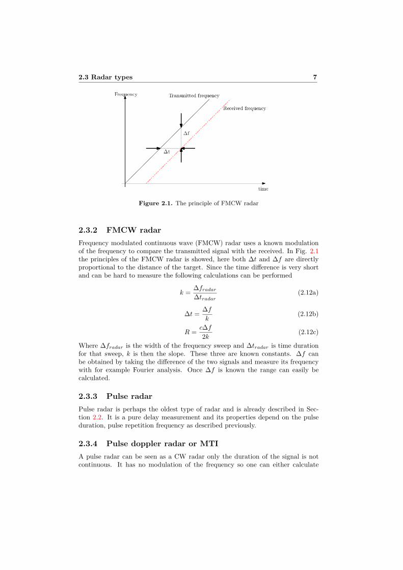
Figure 2.1. The principle of FMCW radar
2.3.2 FMCW radarFrequency modulated continuous wave (FMCW) radar uses a known modulationof the frequency to compare the transmitted signal with the received. In Fig. 2.1the principles of the FMCW radar is showed, here both ∆t and ∆f are directlyproportional to the distance of the target. Since the time difference is very shortand can be hard to measure the following calculations can be performed
k = ∆fradar∆tradar
(2.12a)
∆t = ∆fk
(2.12b)
R = c∆f2k (2.12c)
Where ∆fradar is the width of the frequency sweep and ∆tradar is time durationfor that sweep, k is then the slope. These three are known constants. ∆f canbe obtained by taking the difference of the two signals and measure its frequencywith for example Fourier analysis. Once ∆f is known the range can easily becalculated.
2.3.3 Pulse radarPulse radar is perhaps the oldest type of radar and is already described in Sec-tion 2.2. It is a pure delay measurement and its properties depend on the pulseduration, pulse repetition frequency as described previously.
2.3.4 Pulse doppler radar or MTIA pulse radar can be seen as a CW radar only the duration of the signal is notcontinuous. It has no modulation of the frequency so one can either calculate

8 Radar
the distance using (2.1) or the velocity using (2.11). This give rise to the nameMoving Target Indication (MTI) as stationary targets are ignored when calculatingthe velocity.
2.3.5 MFCW radarIt has been said in this chapter that it is not possible to measure range with a CWradar, but this is not completely true. If a sinusoidal wave is sent with constantfrequency, the transmitted signal will be of the form sin(2πf0t). The reflectedsignal will arrive at the radar T = 2R/c seconds later where R is the one waydistance. The received signal is sin(2πf0(t−T )) and is 2πf0T radians out of phasecompared to the transmitted signal. If the phase difference is measured R can becalculated with
R = c∆φ4πf0
(2.13)
where ∆φ is the phase difference. Because the phase difference is periodic with2π there is a very short unambiguous distance, if ∆φ is substituted with 2π,Run = c/(f02) = λ/2 which is much to short to be of practical use. A Multi-ple Frequency Continuous Wave (MFCW) radar uses two or more parallel signalssimultaneously with slightly different frequencies to increase the unambiguous dis-tance. Assume that two signals are transmitted with f2 = f1+∆f , where ∆f � f1,
s1 = sin(2πf1t+ φ1) (2.14a)
s2 = sin(2πf2t+ φ2) (2.14b)
where φ1 and φ2 are two arbitrary constants. The reflected signals at the radarare
r1 = sin(2π(f1 ± fd1)t+ φ1 −4πf1R
c) (2.15a)
r2 = sin(2π(f2 ± fd2)t+ φ2 −4πf2R
c) (2.15b)
Since ∆f is relative small the two doppler shifts will be approximately the sameand we can write fd = fd1 = fd2. If the received signals are mixed with the corre-sponding ones being sent two new signals are received as
d1 = sin(±2πfdt−4πf1R
c) (2.16a)
d2 = sin(±2πfdt−4πf2R
c) (2.16b)
The phase difference between these two signals can be obtained and R calculatedusing
∆φ = 4π(f2 − f1)Rc
= 4π∆fRc
(2.17a)
R = c∆φ4π∆f (2.17b)

2.3 Radar types 9
The new unambiguous distance is
Run = c
2∆f (2.18)
This radar type is the main model for this master thesis implementation.

Chapter 3
Hardware
In this chapter the hardware platform used in this project is described. All datain this chapter is taken from [4].
3.1 Lyrtech SFF SDR DPThe main aid in this project is the Small Form Factor Software Defined RadioDevelopment Platform (SFF SDR DP) manufactured by the Canadian based com-pany Lyrtech. The platform is a development platform for radio applications andnot used in production. It is a stand alone device and consists of three majormodules each controllable by software instructions. The three modules are:
• Digital processing module
• Data conversion module
• RF module
Each module will be described in the following sections.
3.1.1 Digital processing moduleThe digital processing module is designed with two devices, one DSP and oneFPGA providing the user a choice in the implementation strategy of the signalprocessing. The DSP device is a Texas Instrument component, TMS320DM6446.It is a so called System on Chip (SoC) which means that all functionality that isnormally expected from a microcomputer is implemented directly on the same chip.This chip consists of one DSP and one ARM9 general-purpose processor (GPP),the DSPs core frequency is 594 MHz the ARM9 core frequency is 297 MHz. TheDSP also contains several memories, including 64 32-bits general purpose registers,program RAM and data RAM, and access to external memory.
The FPGA is of type Virtex-4 XC4SX35 provided by Xilinx, it serves as acoprocessor and is also the interface to all the I/O on the platform. From the
11

12 Hardware
digital processing module point of view the data conversion module works as anI/O device. The Virtex-4 XC4SX35 has 96x40 built in Configurable Logic Blocks(CLBs). The communication between the FPGA and the DSP is handled by amodified version of the Video Processing Subsystem protocol, VPSS. It consistsof the Video Processing Front End, VPFE and the Video Processing Back End,VPBE. The VPSS protocol has been modified to handle data other then video tobe transfered between the two modules. The VPFE is used as an input interfaceto the DSP, it is 16 bits deep and works with a 75 MHz clock. The VPBE is anoutput interface from the DSP and works with half the data rate, 37,5 MHz butwith the same bus, 16 bits. The synchronization is already implemented so theVPSS is very easy to use on the SFF SDR DP.
3.1.2 Data conversion moduleThis module has both an Analog to Digital Converter (ADC) and a Digital to Ana-log Converter (DAC). The DAC is a DAC5687 from Texas Instrument and providestwo channel outputs simultaneously. The ADC is of type ADS5500 also from TexasInstruments and can sample up to 125 Mega Samples Per Second (MSPS) with 14bits resolution. On the data conversion module there is an FPGA used to controlthe ADC, DAC and data acquisition, it is of type Virtex-4 XC4VLX25. It cannotbe accessed easily and its purpose is only to control previous stated tasks. Thereis a Phase Locked Loop (PLL) which provides the ADC, DAC and FPGA withtheir desired clock frequencies. A PLL is a control system that keeps the outgoingclocksignal constant in phase and frequency.
3.1.3 RF moduleThe RF (Radio Frequency) module will be divided into one transmitter and onereceiver part.
Transmitter
In Fig. 3.1 a schematic view over the transmitter is shown. The transmitter mixesthe I and Q signals with a carrier wave and transmits the resulting signal over theTX antenna. The I and Q signals are low-pass filtered and mixed with the carrierwave separately, the Q signal is mixed with a phase shifted version of the carrierwave. The carrier wave frequency can be chosen from two intervals, 262-438 MHzor 523-876 MHz. The frequency is kept stable by a PLL.
Receiver
On the receiver side, a three-stage superheterodyne receiver produces a 30 MHzIF (Intermediate Frequency) signal as the final output. Three-stage means thatthe incoming signal is mixed in three stages, see Fig. 3.2. After the first low-passfilter is the first mixer, and its frequency can be chosen between 1600-2500 MHz.The following band-pass filter has a 20 MHz bandwidth and is centered around1575 MHz. Then there is a fixed mixer at 1275 MHz followed by a band-pass filter

3.2 Hardware summary 13
Figure 3.1. The transmitter schematics
centered at 300 MHz, and its bandwidth can be chosen from 5 or 20 MHz. Thelast stage is a 300 MHz fixed frequency mixer followed by a low-pass filter. Thisresults in an IF signal with a 30 MHz carrier frequency.
Figure 3.2. The receiver schematics
3.1.4 Overall functionality and I/OIn the digital processing module there is the possibility to connect a JTAG bothto the DSP and the FPGA. The JTAG provides possibilities both to programthe devices and to debug them. However one can load programs directly to boththe DSP and the FPGA through the Ethernet port but without the possibility todebug. The SFF SDR DP is also equipped with a serial port (RS-232) and audioinputs and outputs. There are also five user defined pushbuttons.
3.2 Hardware summaryTo make it easier for the reader the most important features of the hardware arelisted below.
• Max sample rate of the DAC and ADC is 125 MSPS.
• Carrier frequency can be chosen in the intervalls 262-438 MHz or 523-876MHz.
• The bandwidth of the signal is limited to 20 MHz.


Chapter 4
OFDM
In this chapter the OFDM technique is presented. All information in this chaptercomes from [5].
Multicarrier transmission is widely used by many different techniques and in awide spectra of applications today. The basic idea is to manage to send several bitsof data simultaneously using only one medium of transportation. The transportmedium can for example be a wire, electrical or optical, or the air. The task isto send more then one bit and at the receiver side manage to separate those bitsfrom each other. Through history many techniques have been used which will notbe discussed here. Today the most common technique is OFDM, which is used inalmost all modern high speed radio communication. Since it is so widely used alarge number of relatively cheap components are available.
OFDM is an abbreviation for Orthogonal Frequency Division Multiplexing andis a modulation technique for multicarrier transmission. Instead of using just onecarrier with a high symbolrate OFDM utilize multiple carriers with low symbolrateto achieve the same throughput. Due to the orthogonal property in this multiplex-ing technique the channels can be spaced close together thus achieving a narrowbandwidth.
Figure 4.1. A simplified general structure view of an OFDM system
15

16 OFDM
Fig. 4.1 shows the general structure of an OFDM system. The incoming datastream is multiplexed into parallel streams of data transmitted simultaneously,each component from the incoming data are modulated with a unique frequency.Since these frequencies can be placed very close together, it permits a relativenarrow bandwidth if you compare to other multiplexing techniques with the sameinformation capacity. This figure shows the system at a high level and will bediscussed in more detail in Section 4.2.
4.1 OrthogonalityThe meaning of orthogonality in the OFDM case is based upon the idea that eachcarrier has an integer number of cycles over a symbol period. This is an advantagesince it results in each carrier having a null at the center frequency of each of theother carriers. This results in a minimum Inter Symbol Interference (ISI), ideallyzero interference. The orthogonality property can also be expressed in a moremathematical way according to
1TFFT
TFFT∫t=0
e−i2π∆f(k−k′)tdt ={
1 for k = k′
0 for k 6= k′(4.1)
Here TFFT denotes the duration of one OFDM symbol, ∆f is the frequency spacebetween two neighboring carriers and k and k′ are their carrier numbers, where kcan take values in the range of 1 to the total number of subcarriers.
4.2 OFDM generation
Figure 4.2. A schematic view of the signal in a OFDM transmitter
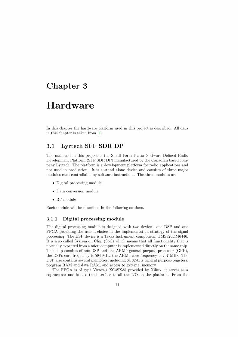
Figure 4.2 shows a schematic view of the transmitter side. The incomingdata is a serial digital signal, it demultiplexes into N parallel streams where Nis the number of subcarriers. Before the Inverse Fast Fourier Transform (IFFT)each component is mapped in the frequency domain, we use Quadrature PhaseShift Keying (QPSK) to map our signals. In QPSK-mapping two binary bits aretranslated into a complex value. Where the first bit determines the real part and
4.2 OFDM generation 17
the second bit determines the imaginary part of the value, see Fig. 4.3. The fourcombinations of those are placed at π/2 phase difference from each other. In figure
Figure 4.3. QPSK bit encoding
4.3 the axis are called I and Q and stands for In-phase (I) and Quadrature-phase(Q), it can be interpreted as the imaginary domain.
The QPSK-mapping generates the following signal in the frequency domain
SBB(f) =N∑k=1
eiγkδ(f − fk) (4.2)
Where γk is the phase received in the QPSK-mapping. The IFFT results in acomplex baseband signal in the time domain:
sBB(t) = F−1 {SBB} =N∑k=1
ei(2πfkt+γk) (4.3)
The signal is then IQ-modulated. This means that the real and the imaginary partof the signal are modulated individually and that the modulating carriers have thesame frequency but differ π/2 in phase. And that the two modulated signals aresummed together before they are transmitted. The sent signal is
s(t) = <{sBB(t)} · sin(2πfct) + ={sBB(t)} · sin(2πfct+ π/2) =
. . . =N∑k=1
sin(2π(fc + fk)t+ γk) (4.4)
where fc is the carrier frequency. At the receiver the reverse process can beimplemented to extract the information sent, but in this project the hardwaredoes not allow this, see Fig. 3.2 in Section 3.1.3. Instead the RF module givesan IF signal which will be sampled and the I and Q separation is performed insoftware. The result however will be the same.


Chapter 5
System
This chapter discusses how the hardware described in Chapter 3 is used and alsothe other components needed to build a complete radar system.
5.1 Overall functionalityThe radar aims to work as a stand alone device. The hardware platform alone doesnot allow to fully achieve this for mainly two reasons. The first reason is that theFPGA and DSP software must be loaded from an outside storage device at everyboot sequence, normally the user loads the programs from a standard PC. Becausethe lack of a display of some kind the only possibility for the user to read the resultfrom the length estimation is to read in the DSP memory, this can be done witha PC. The stand alone property means that all aids to estimate the length mustbe generated within the hardware as well as all the necessary calculations. Figure5.1 shows an overview of all the systems components and how they interact witheach other.
Figure 5.1. Overview of the system.
19

20 System
PRBS
In a Pseudo-Random Binary Sequence, PRBS, the values are random to each otherbut the sequence repeats itself after N samples, normally N is very large and froma user point of view the sequence is interpreted as just random values.
OFDM modulation and IFFT
The values from the PRBS are mapped using the QPSK technique and an 128point IFFT is performed to obtain a time signal. We have chosen to have fourtimes oversampling in order to ensure low ICI while keeping the number of pointsin the FFT/IFFT low. This is achieved by placing the subcarriers on every fourthsample in the Fourier domain. Since we have chosen to use 16 subcarriers andthe number of points in the IFFT is 128, the sample frequency needs to be 40MHz in order to achieve a bandwidth of 20 MHz. The subcarriers are centeredaround zero. This is the first part of Fig. 4.2 and is discussed in more detailin section 4.2. The output signal from the QPSK-mapping is a complex valuedvector. One complex value occupy two vector indexes, the first is the real and thesecond is the imaginary value. All software functions are implemented using thisinformation representation for complex values. This block as well as the PRBSare implemented in the DSP.
Send buffer and upsampling
The FPGA and DSP communicate over a VPSS bus described in Section 3.1.1.Since the output interface from the DSP works with a 37.5 MHz clock which ismuch slower than the clock frequencies in both the DSP and the FPGA a sendbuffer is necessary to eliminate data loss. In the data conversion module the ADCand the DAC are clocked by the same clock source which means that there isno possibility to have them working on different frequencies. The ADC/DAC isset to work at 120 MSPS. This yields that the OFDM subcarriers will be placedat frequencies above 20 MHz resulting in information loss at the receiver sidein the RF module if the DAC frequency where to be equally high. The signalbandwidth cannot exceed 20 MHz due to the filter bandwidths. This fact motivatesan upsampling before the signal is sent to the DAC. The upsampling is done by afactor three to compensate for the too high frequency, this will place the signal inthe right frequency band.
Transmitter signal processing
This block takes the upsampled I and Q signals through the DAC, the DAC runsin dual channel mode which means that the two signals are sampled individually.The continuous-time signals are then IQ-modulated, i.e. multiplied with a RFcarrier wave combining the I and Q signal to one resulting signal. The resultingsignal is the one that will be transmitted using the RF output. For a more detailedview see the last part of Fig. 4.2. Fig. 3.1 shows the same information but withoutthe DACs.

5.1 Overall functionality 21
Receiver signal processing
The receiver signal processing block is the hardware part consisting of severalfilters and frequency operations, see Fig. 3.2 for a detailed view and discussion.
ADC
As previously stated the ADC samples at 120 MSPS resulting in a four timesoversampling. The IF signals has frequency components in the range of 20-40MHz, and thus there is no aliasing.
Receiver buffer
The signal is now sampled and ready to be further processed digitally by eitherthe FPGA or the DSP. In this implementation all of the processing will take placeinside the DSP leaving the FPGA only to buffer the incoming signal and send itover the VPSS bus to the DSP. The DSP input interface is twice as fast as theoutput, 75 MHz but still to slow to read the signal in real time, this is why a bufferis used at the receiver side the same way it is used on the transmitter side.
Software signal processing
Fig. 5.2 shows a detailed view over this block. The IQ-separation is done using
Figure 5.2. A detailed view of the software signal processing block.
a sinus wave at 30 MHz to transfer the IF signal to the right frequencies and toobtain the two I and Q signals.
In = rn sin(2π30 · 106n) (5.1a)
Qn = rn cos(2π30 · 106n) (5.1b)
Here rn is the output signal from the ADC. After the frequency mixing boththe I and Q signals contain unwanted frequency components at 30+30 MHz with20 MHz bandwidth, the wanted component is placed at 30-30 MHz also with 20MHz bandwidth. To eliminate this two low-pass filters each with 15 MHz cutofffrequency are used on the separated signals. This implementation uses two fifthorder Butterworth filters.

22 System
The downsampling is performed in correspondence to the upsampling at thetransmitter side. After the downsampling, the signals have the same number ofsamples and bandwidth which is required for an adequate signal processing in thefollowing blocks. The last step in this block is an FFT that takes the I and Qsignals and transform them to the frequency domain. The FFT returns a complexvalued vector coded in the same way as was described when the OFDMmodulationand IFFT were discussed. All of these operations and the two last blocks are allimplemented using the DSP.
Phase estimation
All our length estimation algorithms have the phase difference as an input ar-gument, this data is calculated in this block. The phase difference refers to thedifference between the transmitted signal and the received signal. From Fig. 5.1one can see that the sent signal is connected to the phase estimation block fromthe OFDM modulation and IFFT block. The signal is taken before the IFFT sothe phase estimation block has two input signals, both in the frequency domain.The phase difference is estimated by using
ϕ(f) = arctan(={RBB(f)SBB(f)∗}<{RBB(f)SBB(f)∗}
)(5.2)
where ∗ denotes the complex conjugate. This function is only called for indexes ncorresponding to the 16 interesting subcarrier frequencies, arctan is extended toinclude the whole imaginary space, i.e. the value range is [−π, π].
Length estimation
This block uses the phase information to estimate the length to the target sur-face. The sensor uses three different methods which all are discussed in detail inchapter 7.
5.2 Software implementationThe software for the DSP is written in C using CodeComposer. The software forthe FPGA is written in C using ImpulseC and VHDL using ISE. A program topresent the results on a PC were produced. This program was written in C++using Visual C++.
In appendix A the flowcharts over the DSP and FPGA programs are attached.
5.3 Measurement rigThe hardware platform comes with isotropic antennas radiating in all directionswhich is not suitable for use in radar context. In Section 3.1.3 the possible fre-quencies are given and the chosen frequency band is 510-750 MHz. Since thesefrequencies coincide with television broadcasting we used television antennas. The

5.3 Measurement rig 23
Figure 5.3. A picture of the equipment used for measurements
two antennas being used are of the same type and has a antenna gain, see equa-tion (2.4), of 10-14 dB according to [2]. The needed components for a stand alonemeasurement rig are the hardware platform, two antennas and a computer to loadprograms into the hardware but also to be able to visualize the result since thehardware is not equipped with any sort of display. These three components aremounted on a rig which with the aid of a forklift provides mobility. See figure 5.3for a picture of the rig. Since the frequency band corresponds to a wavelengthband of 40-59 cm relative irregular targets can be used, although throughout allmeasurements a metal plate with a flat surface have been used as target. Onecan read about the results of the measurements further on in this report. Whenperforming a measurement the correct distance is measured using a tape measurewith centimeter accuracy.
24 System
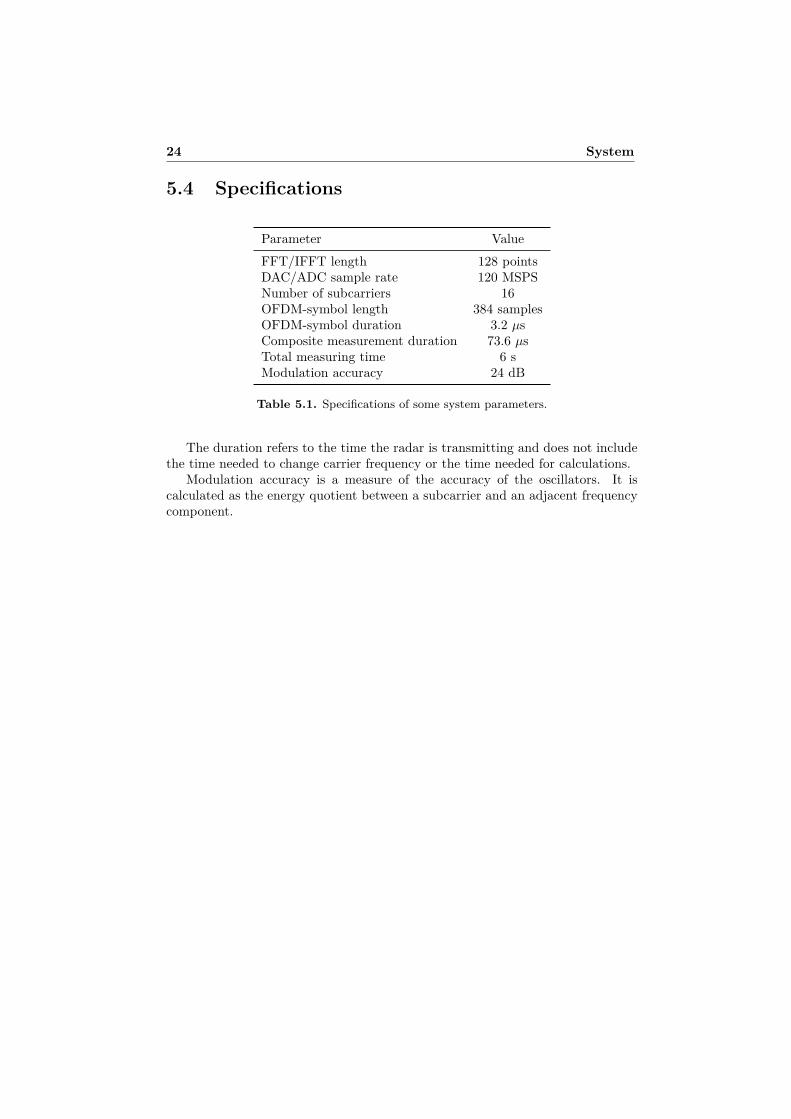
5.4 Specifications
Parameter ValueFFT/IFFT length 128 pointsDAC/ADC sample rate 120 MSPSNumber of subcarriers 16OFDM-symbol length 384 samplesOFDM-symbol duration 3.2 µsComposite measurement duration 73.6 µsTotal measuring time 6 sModulation accuracy 24 dB
Table 5.1. Specifications of some system parameters.
The duration refers to the time the radar is transmitting and does not includethe time needed to change carrier frequency or the time needed for calculations.
Modulation accuracy is a measure of the accuracy of the oscillators. It iscalculated as the energy quotient between a subcarrier and an adjacent frequencycomponent.

Chapter 6
Mathematical description
In the following sections a qualitative analysis of the system is conducted. Someidealizations and simplifications are made in order to arrive at expressions usablein our length estimation algorithms.
6.1 Transmitter
The transmitter’s task is to mix the baseband I and Q signals with a carrier to getone RF-signal. This procedure was discussed earlier in Section 4.2. By comparingthe schematics of a general OFDM transmitter, Fig. 4.2, and the schematics of thetransmitter used in this project, Fig. 3.1, we can see that they are very similar.This suggests that equation (4.4) can be used to describe the transmitter withgood accuracy. In this project N is set to 16. Since only the frequency and notthe phase of the oscillators of the RF module are known, the transmitted signalwill be
s(t) =16∑k=1
sin(2π(fk + ftx)t+ γk + ξtx) (6.1)
where ftx is the frequency of the transmitter oscillator and ξtx its phase, fk arethe baseband frequencies of the OFDM subcarriers and γk is the phase from theQPSK-mapping. These frequencies are described by the linear function
fk = ∆fk − foffset (6.2)
where foffset is the frequency of the first subcarrier and ∆f is the distance betweenthe subcarriers.
How the transmitted signal appears in the frequency domain is illustrated inFig. 6.1.
25

26 Mathematical description
Figure 6.1. The transmitted signal in the frequency domain.
6.2 ReceiverIdeally the signal received at the antenna is just a time delayed version of thetransmitted signal
r(t) = s(t−∆t) =16∑k=1
sin(2π(fk + ftx)(t−∆t) + γk + ξtx) (6.3)
where the time delay is a function of the distance to be measured, according to
∆t = l/c (6.4)
The time delay can be rewritten as a phase shift. Let
ψk = 2π(fk + ftx)∆t = 2π(fk + ftx)lc
(6.5)
The received signal can then be written as
r(t) =16∑k=1
sin(2π(fk + ftx)t− ψk + γk + ξtx) (6.6)
In the receiver the signal is mixed with three oscillators at different frequen-cies. After each mixing the signal passes through a filter that removes unwantedfrequency components. If we consider the filters ideal, i.e. only the wanted com-ponents remain, it greatly simplifies the equations.
Since the filters remove half of the signal’s energy the amplitude will decreaseafter each mixer. To compensate this the receiver is equipped with two amplifiers.In this discussion however, we’re only interested in the frequency and the phaseof the signal. To further simplify the equations we consider the signals amplitudeto be constant.
After the first mixer and filter the signal is
r1(t) =16∑k=1
sin(2π(−fk − ftx + frx1)t+ ψk − γk − ξtx + ξrx1) (6.7)
The frequency of the first oscillator is frx1 and its phase ξrx1. Since there is noway of determining the phase of the individual oscillators it is convenient to write

6.3 Length information 27
their combined phase shift, as well as other phase shifts, as ξ = ξtx − ξrx1 + ... .This signal is mixed with the second oscillator and filtered with the filter set to 20MHz bandwidth. The result is
r2(t) =16∑k=1
sin(2π(−fk − ftx + frx1 − frx2)t+ ψk − γk − ξ) (6.8)
After the last hardware mixer and filter the signal is
r3(t) =16∑k=1
sin(2π(fk + ftx − frx1 + frx2 + frx3)t− ψk + γk + ξ) (6.9)
After the third oscillator the signal is sampled and IQ-separation is performedin software, using frx4, as described in (5.1). Considering the subsequent filter-ing ideal and pretending that the signal is still continuous we get the followingIQ-separated signal
I(t) =16∑k=1
cos(2π(fk + ftx − frx1 + frx2 + frx3 − frx4)t− ψk + γk + ξ) (6.10a)
Q(t) =16∑k=1
sin(2π(fk + ftx − frx1 + frx2 + frx3 − frx4)t− ψk + γk + ξ) (6.10b)
For I(t) and Q(t) to be at baseband frequency the following relationship must hold
ftx − frx1 + frx2 + frx3 − frx4 = 0 (6.11)
This can be achieved by matching ftx and frx1. (frx2, frx3 and frx4 have fixedfrequencies.) Unfortunately this relationship will not always hold due to inaccura-cies in the oscillators. However the deviation is rather small and (6.11) will almosthold.
The I(t) and Q(t) signals can then be seen as one complex baseband signal
rBB(t) = I(t) + iQ(t) =16∑k=1
ei(2πfkt−ψk+γk+ξ) (6.12)
The transform will then be
RBB(f) = F {rBB(t)} =16∑k=1
ei(−ψk+γk+ξ)δ(f − fk) (6.13)
6.3 Length informationThe length is proportional to the change in phase from the transmitted signalto the received signal, ψk. To remove some unwanted components, the Fourier

28 Mathematical description
transform of the received signal, (6.13), is multiplied by the complex conjugate ofthe transmitted signal, (4.2). Resulting in
RBB(f)(SBB(f))∗ =16∑k=1
ei(−ψk+ξ)δ(f − fk) (6.14)
We can only measure the total phase for each subcarrier
ϕk = −ψk + ξ = −2π(fk + ftx)l/c+ ξ (6.15)
and separating ψ from ξ has turned out to be nontrivial. Several methods for doingthis and estimating the length has been suggested and are presented in Chapter 7.
The disturbing phase component, ξ, originates from the oscillators phase atthe beginning of a measurement and phase shifts due to delays in the system.Therefore it will be constant through each measurement but random betweenmeasurements.
Early in the project, before we had access to the hardware, ξ was believedonly to originate from delays in the system, and thereby be constant betweenmeasurements. During this time method 3 and 4 for length estimation, discussedin Chapter 7, were developed. They require ξ to be known, but since that is notthe case they will not work on this hardware. We still include them in this reportbecause they might work on a different hardware platform.
6.4 Multiple echoesAs mentioned before, (6.14) is valid only when one echo is received, i.e. the receivedsignal is a time delayed version of the signal sent. In real measurements there willmost likely be more than one echo present. For example, even in the simplestoiltank the oil surface as well as the bottom of the tank will result in echoes. Amore realistic way to express the received signal is to convolve the sent signalwith two, or more, time delayed Dirac delta functions with different amplitudes,resulting in
r(t) = s(t) ∗(
M∑m=1
amδ(t− lm/c))
(6.16)
Where M is the number of echoes and am is the amplitude of echo m. Using this,the expression corresponding to (6.14) will be
RBB(f)(SBB(f))∗ =16∑k=1
M∑m=1
amei(−ψk,m+ξ)δ(f − fk) (6.17)
The relationship between the measured phase and the length we want to mea-sure is no longer linear. The measured phase will be
ϕk = arg(
M∑m=1
ame−iψk,m
)+ ξ (6.18)
6.4 Multiple echoes 29
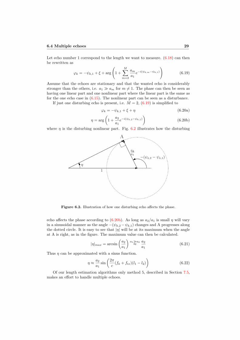
Let echo number 1 correspond to the length we want to measure. (6.18) can thenbe rewritten as
ϕk = −ψk,1 + ξ + arg(
1 +M∑m=2
ama1e−i(ψk,m−ψk,1)
)(6.19)
Assume that the echoes are stationary and that the wanted echo is considerablystronger than the others, i.e. a1 � am for m 6= 1. The phase can then be seen ashaving one linear part and one nonlinear part where the linear part is the same asfor the one echo case in (6.15). The nonlinear part can be seen as a disturbance.
If just one disturbing echo is present, i.e. M = 2, (6.19) is simplified to
ϕk = −ψk,1 + ξ + η (6.20a)
η = arg(
1 + a2
a1e−i(ψk,2−ψk,1)
)(6.20b)
where η is the disturbing nonlinear part. Fig. 6.2 illustrates how the disturbing
Figure 6.2. Illustration of how one disturbing echo affects the phase.
echo affects the phase according to (6.20b). As long as a2/a1 is small η will varyin a sinusoidal manner as the angle −(ψk,2−ψk,1) changes and A progresses alongthe dotted circle. It is easy to see that |η| will be at its maximum when the angleat A is right, as in the figure. The maximum value can then be calculated.
|η|max = arcsin(a2
a1
)a1�a2≈ a2
a1(6.21)
Thus η can be approximated with a sinus function.
η ≈ a2
a1sin(
2πc
(fk + ftx)(l1 − l2))
(6.22)
Of our length estimation algorithms only method 5, described in Section 7.5,makes an effort to handle multiple echoes.

30 Mathematical description
6.5 PerformanceTo increase the ability to separate echoes from each other we need to increase thebandwidth.
The development platform used in this project has a bandwidth limitation of20 MHz which is very low in radar context. In an effort to increase bandwidth, andthereby resolution, we make several measurements with different carrier frequen-cies and merge the results, see Section 7.5.1. In our implementation we make upto 23 partly overlapping measurements, which gives us an effective bandwidth ofabout 240 MHz. Compared to level gauging radars in production with a bandwidthof 1.5 GHz this is still quite low. Hence, we do expect poorer resolution.
6.6 Unambiguous distanceSince we are dealing with periodic signals there is a maximum length we canmeasure before the result becomes ambiguous, as illustrated in Fig. 6.3. Our
Figure 6.3. The distance between the dots is the unambiguous distance.
radar is supposed to measure distances up to 30 m. Thus the unambiguous lengthmust be greater than 60 m since the radio wave has to travel forth and back.
For a single sinus wave, sin(2πft), the unambiguous distance is equal to thewave length. In this case we have 16 sinus waves at different frequencies. Assumethat the phase equals zero for all waves at t = 0, then the unambiguous distancewill correspond to the lowest t > 0 for which all phases equals zero, i.e.,
2πfit− 2πni = 0 , i = 1, 2 . . . 16 (6.23)
where ni is the number of periods the wave has traveled. The difference betweenthe phases will also be zero, i.e.,
(2πfit− 2πni)− (2πfjt− 2πnj) = 0 , i, j = 1, 2 . . . 16 (6.24)
This can be rewritten ast = ni,j
fi − fj(6.25)
where ni,j = ni − nj . Since we have equal distances between the frequencies, ∆f ,we can make the following simplification for all combinations of i and j in (6.25):
t = ni,j(i− j)∆f (6.26)
ni,j = (i− j)n1,2 (6.27)

6.7 MatLab model 31
If we let n = n1,2 and insert (6.27) in (6.26) we get
t = n
∆f (6.28)
The unambiguous period time corresponds to n = 1 and is now known. In thisproject we have ∆f= 1.25 MHz. We can calculate the corresponding distance
Runambiguous = c · t|n=1 = c
∆f = 240 m (6.29)
where c is the speed of light. Thus ambiguity will not be a problem in this project.
6.7 MatLab modelTo be able to develop and evaluate methods of estimating lengths without needingaccess to the actual hardware, simulation models of the transmitter and receiverwere built in MatLab. These models were built by following the system descriptionin Chapter 5. Since the exact characteristics of the hardware filters are unknownthey were approximated with Butterworth filters of matching cutoff frequencies.The distance to be measured is modeled as a time delay. We have added thepossibility to simulate multiple echoes and add noise to the signal.


Chapter 7
Length estimation
Since we want to measure the distance to the surface in a tank, we have developedfive different ways to estimate this length and they will be presented one by onein the following sections.
Note that due to delays in the hardware the estimated length will have aconstant offset that needs to be calibrated.
7.1 Method 1 - Linear regressionFrom (6.15) we know that the phase is very similar to a straight line. It can bewritten as a function of frequency.
ϕ(f) = −2πfl/c+ ξ (7.1)
In the implementation it is important that the phase is modified to this straightline. When calculating the phase in the MatLab models or in the DSP with ourphase-extraction-function the returned value is in the range of [−π, π]. Since weknow that the phase is supposed to decrease with increasing frequencies it can beunwrapped. This is illustrated in Fig. 7.1 As the measured distance increases theslope of the phase becomes steeper. If the slope changes 2π+ ε between two phasemeasurements the unwrapping function will interpret it as if the change is ε, hencethe result will be ambiguous. This issue was further discussed in Section 6.6.
One can extend (7.1) to all 16 frequencies in a measurement:ϕ1ϕ2...ϕ16
= −2πlc
f1f2...f16
+ ξ (7.2)
It is easy to see that this is a least square problem if we write (7.2) in the following
33

34 Length estimation
Figure 7.1. Left: The phase is in the intervall [−π, π]. Right: The phase is unwrappedand now extends beyond −π.
way: f1 1f2 1...f16 1
(− 2π
c lξ
)=
ϕ1ϕ2...ϕ16
(7.3)
The standard solution to a least square problem of the form Ax = B isx = (ATA)−1ATB [6]. Identification in (7.3) gives:
ATA =(f2
1 + f22 + . . .+ f2
16 f1 + f2 + · · ·+ f16f1 + f2 + . . .+ f16 16
)(7.4a)
(ATA)−1 = 1|ATA|
(16 −(f1 + . . .+ f16)
−(f1 + . . .+ f16) f21 + . . .+ f2
16
)(7.4b)
|ATA| = 16(f21 + f2
2 + . . .+ f216)− (f1 + f2 + . . .+ f16)2 (7.4c)
ATB =(f1ϕ1 + f2ϕ2 + . . .+ f16ϕ16
ϕ1 + ϕ2 + . . .+ ϕ16
)(7.4d)
(ATA)−1ATB =
1|ATA|
(16(f1ϕ1 + . . .+ f16ϕ16)− (f1 + . . .+ f16)(ϕ1 + . . .+ ϕ16)
−(f1 + . . .)(f1ϕ1 + . . .) + (f21 + . . .)(ϕ1 + . . .)
)(7.4e)
(7.3) combined with (7.4e) gives the approximated distance to the echo and back.The length can be written as:
l = − c
2π|ATA| (16(f1ϕ1 + . . .+ f16ϕ16)− (f1 + . . .+ f16)(ϕ1 + . . .+ ϕ16)) (7.5)
7.2 Method 2 - Two point differenceA simple way to calculate the distance is to only look at two frequencies, f1 andf2, and their respective phase, ϕ1 and ϕ2. From (7.1) we know that for a certain

7.3 Method 3 - Nearest integer 35
length the phase is linearly proportional to the frequency. This also means that thedecrease in phase between two subcarriers with different frequencies is proportionalto the increase in frequency, i.e.,
− (ϕ1 − ϕ2) = 2π(f1 − f2)l/c+ ξ − ξ (7.6)
The length can then be calculated by
l = c
2π ·ϕ2 − ϕ1
f1 − f2(7.7)
This is very similar to the MFCW radar described in Section 2.3.5.Since we have 16 frequencies we can calculate the length for several combina-
tions of two and then take the mean to reduce the influence of noise. With 16frequencies we can find (16 − 1)! ≈ 1.3077 · 1012 combinations of two. But sincewe want a reasonably fast algorithm we have chosen only to look at adjacent fre-quencies. We do not believe this will affect the outcome significantly. We can thencalculate the length like this
l = c
2π · 15
15∑i=1
ϕi+1 − ϕifi − fi+1
(7.8)
7.3 Method 3 - Nearest integerAs mentioned before, methods 3 and 4 do not work on the hardware used inthis project. These methods require the system delay to be constant betweenmeasurements and ϕ(f) = 0 when l = 0. Let
ξ = ∆− 2πn (7.9)
where ∆ is the delay in the system and n is the number of wavelengths the wavehas propagated. The measured phase can then be written as
ϕ(f) = −2πfl/c+ ∆− 2πn (7.10)
Methods 3 and 4 do not require the phase to be unwrapped, i.e. n can differbetween subcarriers.
The approach here is to ”guess” n and use that we know that n is an integer.But instead of just guessing one value we try all likely values of n and pick theone most probable.
First we rewrite (7.10) in two ways, as
l = c
2πf (ϕ+ 2πn−∆) (7.11a)
n = f · lc− ∆− ϕ
2π (7.11b)
In (7.11a) we can calculate l for a given frequency and n and in (7.11b) we cancalculate n if the length is known.

36 Length estimation
Let us make N guesses for n belonging to the first subcarrier and calculate thecorresponding lengths, as
li,1 = c
2πf1(ϕ1 + 2πni,1 −∆1) , i = 1, 2, . . . , N (7.12)
If we insert li,1 in (7.11b) we can calculate
n̂i,j = fj · li,1c
− ∆j − ϕj2π , ∀i , j = 1, 2, . . . , 16 (7.13)
where j denotes the current subcarrier. In the ideal case n̂i,j will be an integer forthe i corresponding to the correct length. But since we have noisy measurements,this is not the case. Instead we pick the i where n̂i,j is nearest integer.
imin = arg mini
16∑j=2
(n̂i,j − [n̂i,j ])2 (7.14)
We now know which one of the guessed n:s that is correct and we can use it tocalculate the estimated length
l = 116
16∑j=1
limin,j = 116
16∑j=1
c
2πfj(ϕj + 2πnimin,j −∆j) (7.15)
7.4 Method 4 - Least varianceOur fourth algorithm for estimating the length is very similar to the third. Itjust includes an extra step. After calculating n̂i,j in (7.13) we take their nearestintegers and calculate the corresponding lengths.
li,j = c
2πfj(ϕj + 2π[n̂i,j ]−∆j) , ∀i, j (7.16)
And then we pick the i for which the length has the smallest variance over j.
imin = arg mini
V ar(li,j) (7.17)
where, according to [6], the variance is estimated by
V ar(li,j) =
∑j
l2i,j −
(∑j
li,j
)2
16
16− 1 (7.18)
Finally we get our length by using (7.15).

7.5 Method 5 - Phase FFT 37
7.5 Method 5 - Phase FFTThe methods described above perform well in the one echo case but they can nothandle multiple echoes because they assume only one echo is present. In method 5we do not make this assumption. Let us look at (6.17) where multiple echoes areconsidered. Since we’re only interested in the phase difference for the subcarrierswe can consider it to be a discrete function only containing these 16 values.
d16k =
M∑m=1
amei(−ψk,m+ξ) , k = 1, 2, . . . , 16 (7.19)
This way d16k can be seen as a superposition of periodic functions with different
amplitude and frequency, where the frequencies are proportional to the distances tothe reflecting objects. The idea is to separate the echoes by calculate the DiscreteFourier Transform of d16
k , using the Fast Fourier Transform algorithm (FFT), andlook in the Fourier domain. A peak search on the spectra will reveal the frequenciesof the periodic functions and thereby their corresponding distances.
To illustrate this we assume that k is not limited to 16 values. Instead k ∈ Z,where Z denotes the set of all integers. If we include this and (6.15) and (6.2) in(7.19) we get
d∞k =M∑m=1
amei(−2π(∆fk−foffset+ftx)lm/c+ξ) , k ∈ Z (7.20)
This way the Discrete-Time Fourier Transform, DTFT [7], can be used to receivethe Fourier transform
D∞(θ) = Fdtft {(d∞k )∗} =M∑m=1
ame−iAm
∞∑r=−∞
2πδ(θ − ∆f
c
(lm + c
∆f r))(7.21)
Here θ is the normalized frequency and Am = 2π(foffset − ftx)lm/c + ξ. Notethat the transform of the complex conjugate of dk is calculated. This is becausewe want an increase in length to result in a larger frequency, instead of a decreasein frequency, in order to make interpretation more intuitive.
D∞(θ) is periodic with period 1. It is easy to see that this periodicity corre-sponds to the unambiguous length discussed in Section 6.6. This means that weonly need to look at one period.
D∞(θ) =M∑m=1
2πame−iAmδ(θ − ∆f
clm
), θ ∈ [0, 1] (7.22)
This is assuming that all reflecting objects are close enough to avoid ambiguity.Since each echo is represented by one Dirac impulse in the Fourier domain the
lengths can be found by making a peak search of the spectra of (7.22).
|D∞(θ)|2 =M∑m=1|2πam|2δ
(θ − ∆f
clm
), θ ∈ [0, 1] (7.23)

38 Length estimation
If a peak is found at θpeak the length is l = θpeakc/∆f .In the discussion above we have an infinite number of samples, k ∈ Z. This is
of course not the case. Instead we have a truncated signal with N samples whichcorresponds to multiply d∞k with a rectangular function
wk ={
1 , k = 0, 1, . . . , N − 10 , otherwise
, W (θ) = Fdtft {wk} = sin(πNθ)sin(πθ) e
iπ(N−1)θ
(7.24)giving us
dNk = d∞k wk , DN (θ) = Fdtft{dNk}
= 12π (D∞ ∗W )(θ) (7.25)
Since we use FFT and not TDFT to calculate the transform we get a sampledversion of the transform.
DNn = DN (θ)
∣∣θ=n/N (7.26)
The received spectrum will then be
|DNn |2 =
M∑m=1
a2m
sin2(πN(n/N − ∆fc lm))
sin2(π(n/N − ∆fc lm))
(7.27)
Where the relationship between n and corresponding length is
l = c
N∆f n (7.28)
This means that instead of Dirac impulses we get wide peaks with side lobeswhere the center of the peak marks the wanted distance. The case were N = 16is illustrated in Fig. 7.2. With only 16 samples we get one sample every 15 m. Ofcourse, this is not enough.
Figure 7.2. One echo at 70 m and N = 16

7.5 Method 5 - Phase FFT 39
7.5.1 Increasing bandwidthTo increase the number of points we need to increase the bandwidth. The hardwareused in this project only supports 20 MHz bandwidth. The only way to increasebandwidth is to make several measurements at different carrier frequencies andthen merge the result. The idea is to choose carrier frequencies so that the mea-surements are edge to edge and the distance between all subcarriers are ∆f . Thisis accomplished by stepping the carrier frequency by 20 MHz. We have chosen toincrease the bandwidth twelve times to 240 MHz and thus increase the number ofsamples to 192, i.e one sample every 1.25 m. However, since ξ is random betweenmeasurements dk will experience a phase shift every 16th sample. We have usedtwo approaches to counter these phase shifts.
Figure 7.3. Phase from measurement with target at 1.97 m.
Figure 7.4. Resulting phase vector after performed merging of measurements.
In the first approach we assume that the wanted echo is significantly strongerthan the disturbing echoes and that the phase of dk is as in (6.19). In Fig. 7.3 we
40 Length estimation
can see that the phase appears as 12 straight lines, one for each measurement. Dueto ξ their offsets are random. We want to remove the randomness and thus makethe phase of the composite measurement into one straight line. To accomplish thiswe calculate the mean slope of the 12 measurements and then adjust their offsetsso they fit a line with that slope. This has been done in Fig 7.4.
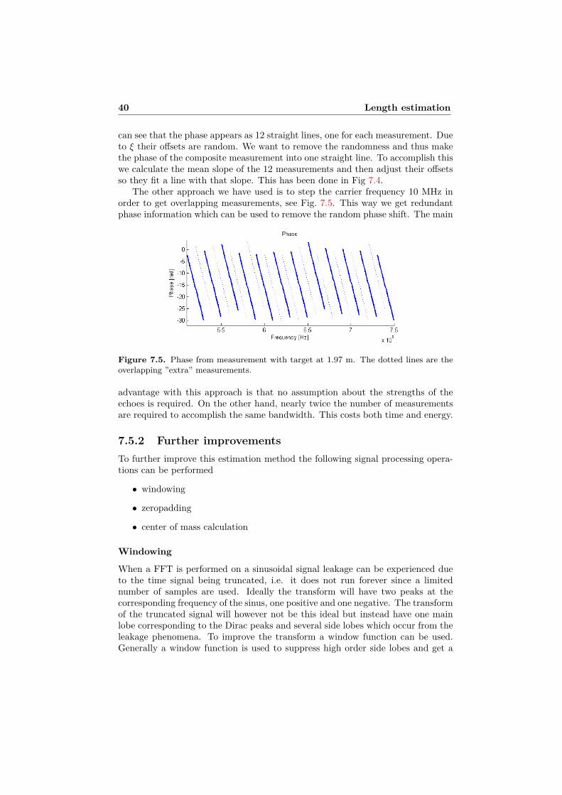
The other approach we have used is to step the carrier frequency 10 MHz inorder to get overlapping measurements, see Fig. 7.5. This way we get redundantphase information which can be used to remove the random phase shift. The main
Figure 7.5. Phase from measurement with target at 1.97 m. The dotted lines are theoverlapping ”extra” measurements.
advantage with this approach is that no assumption about the strengths of theechoes is required. On the other hand, nearly twice the number of measurementsare required to accomplish the same bandwidth. This costs both time and energy.
7.5.2 Further improvementsTo further improve this estimation method the following signal processing opera-tions can be performed
• windowing
• zeropadding
• center of mass calculation
Windowing
When a FFT is performed on a sinusoidal signal leakage can be experienced dueto the time signal being truncated, i.e. it does not run forever since a limitednumber of samples are used. Ideally the transform will have two peaks at thecorresponding frequency of the sinus, one positive and one negative. The transformof the truncated signal will however not be this ideal but instead have one mainlobe corresponding to the Dirac peaks and several side lobes which occur from theleakage phenomena. To improve the transform a window function can be used.Generally a window function is used to suppress high order side lobes and get a
7.5 Method 5 - Phase FFT 41
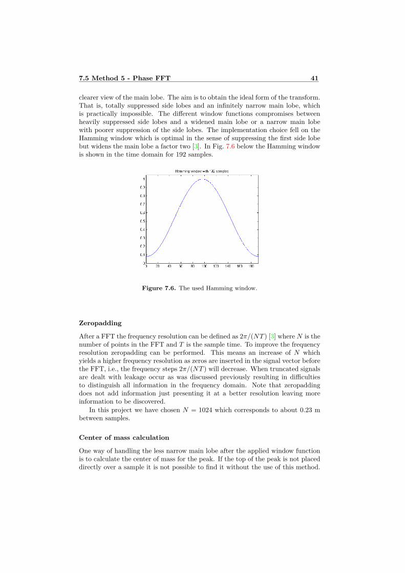
clearer view of the main lobe. The aim is to obtain the ideal form of the transform.That is, totally suppressed side lobes and an infinitely narrow main lobe, whichis practically impossible. The different window functions compromises betweenheavily suppressed side lobes and a widened main lobe or a narrow main lobewith poorer suppression of the side lobes. The implementation choice fell on theHamming window which is optimal in the sense of suppressing the first side lobebut widens the main lobe a factor two [3]. In Fig. 7.6 below the Hamming windowis shown in the time domain for 192 samples.
Figure 7.6. The used Hamming window.
Zeropadding
After a FFT the frequency resolution can be defined as 2π/(NT ) [3] where N is thenumber of points in the FFT and T is the sample time. To improve the frequencyresolution zeropadding can be performed. This means an increase of N whichyields a higher frequency resolution as zeros are inserted in the signal vector beforethe FFT, i.e., the frequency steps 2π/(NT ) will decrease. When truncated signalsare dealt with leakage occur as was discussed previously resulting in difficultiesto distinguish all information in the frequency domain. Note that zeropaddingdoes not add information just presenting it at a better resolution leaving moreinformation to be discovered.
In this project we have chosen N = 1024 which corresponds to about 0.23 mbetween samples.
Center of mass calculation
One way of handling the less narrow main lobe after the applied window functionis to calculate the center of mass for the peak. If the top of the peak is not placeddirectly over a sample it is not possible to find it without the use of this method.

42 Length estimation
If nmax is the n for which the amplitude of the spectrum has its maximum, themass center can be obtained using the formula below:
nmc =∑nmax+M+n=nmax−M− n · |D
Nn |2∑nmax+M+
n=nmax−M− |DNn |2
(7.29)
Here M− and M+ are the number of samples on each side of nmax, these aredesign variables and affect the outcome of the mass center calculation. In ourimplementation M− and M+ are chosen dynamically in order to include as muchas possible of the main peak without including any sidelobes. The calculation isillustrated in Fig. 7.7.
Figure 7.7. Center of mass calculation. The green * mark the samples included inthe calculation and the red + marks the result. (The figure does not show the wholespectrum.)
7.6 Evaluation of algorithmsIn this section we will evaluate the length estimation algorithms using data fromsimulations in MatLab. Methods 3 and 4 will not be included since they do notwork on the hardware used in this project. Method 5 will be treated as twoseparate methods. One for each approach on how to merge measurements intoone composite measurement. The approach where the measurements are edge toedge is called 5.1 and the one with overlapping measurements is called 5.2.
Methods 1 and 2 can estimate a length using one measurement with 16 subcar-riers, i.e. one OFDM-symbol, while method 5.1 and 5.2 needs 12 and 23 measure-ments respectively to form a composite measurement. This means that methods5.1 and 5.2 have access to more data when length estimation is done. In order to

7.6 Evaluation of algorithms 43
make a more fair comparison between the methods we let methods 1 and 2 esti-mate the length for each of the 23 measurements in the composite measurementand then present the mean value as the estimated length. In Table 7.1 we can seethat the standard deviation decreases for methods 1 and 2 if the whole compositemeasurement is included.
Std.dev Method 1 Method 2(mm) (mm)
σ1 11.33 16.83σ12 3.30 4.90σ23 2.40 3.51
Table 7.1. Standard deviation for simulated measurements with one echo and no noise.Standard deviation for composite measurements with 1, 12 and 23 measurements arelisted.
All following comparisons in this chapter are based on composite measurementsthat consist of 23 measurements. Methods 1, 2 and 5.2 utilize all 23 measurementwhile method 5.1 use the 12 measurements that are edge to edge. In the simu-lations, the length has been stepped from 0 to 30 m with a step length of 0.2 mand 20 composite measurements have been conducted at each length. To highlighttrends in the error, the mean of these 20 measurement is presented in the figuresin this section. To make the figures more readable offsets have been added to theerrors.
Table 7.2 lists the standard deviation for the methods. It is clear that when adisturbing echo is present method 5.1 does not perform as well as the others.
Standard deviation of error, σ (mm)Dist. echo No No 1% at 25 m 1% at 25 m 10% at 25 mSNR No noise 0 dB 20 dB 0 dB 0 dBMethod 1 2.40 4.61 2.54 4.85 14.62Method 2 3.51 8.10 3.50 8.06 15.59Method 5.1 3.62 7.53 7.69 10.16 70.53Method 5.2 3.90 6.92 3.79 7.18 19.89
Table 7.2. Standard deviation for the error in length estimation of simulated measure-ments.
Fig. 7.8 shows the result when only one echo is present. We can see that allfour methods are affected by the noise but that the error is still less than ±1 cm.In Fig. 7.9 a disturbing echo at 25 m with 1% strength compared to the mainecho i added. This weak disturbing echo does no seem to affect the performance ofmethods 1 and 2. Method 5.1 on the other hand has problems with lengths around10 m and method 5.2 has problems when the two echoes are close together.
From Section 6.4 we know that one relatively weak disturbing echo affects themeasured phase in a sinusoidal manner, see (6.22). When the distance between
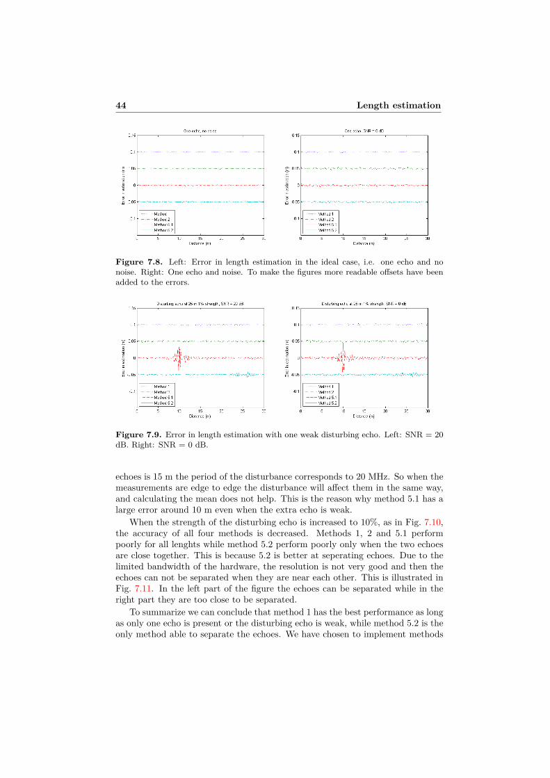
44 Length estimation
Figure 7.8. Left: Error in length estimation in the ideal case, i.e. one echo and nonoise. Right: One echo and noise. To make the figures more readable offsets have beenadded to the errors.
Figure 7.9. Error in length estimation with one weak disturbing echo. Left: SNR = 20dB. Right: SNR = 0 dB.
echoes is 15 m the period of the disturbance corresponds to 20 MHz. So when themeasurements are edge to edge the disturbance will affect them in the same way,and calculating the mean does not help. This is the reason why method 5.1 has alarge error around 10 m even when the extra echo is weak.
When the strength of the disturbing echo is increased to 10%, as in Fig. 7.10,the accuracy of all four methods is decreased. Methods 1, 2 and 5.1 performpoorly for all lenghts while method 5.2 perform poorly only when the two echoesare close together. This is because 5.2 is better at seperating echoes. Due to thelimited bandwidth of the hardware, the resolution is not very good and then theechoes can not be separated when they are near each other. This is illustrated inFig. 7.11. In the left part of the figure the echoes can be separated while in theright part they are too close to be separated.
To summarize we can conclude that method 1 has the best performance as longas only one echo is present or the disturbing echo is weak, while method 5.2 is theonly method able to separate the echoes. We have chosen to implement methods

7.6 Evaluation of algorithms 45
Figure 7.10. Error in length estimation with one disturbing echo.
1, 2 and 5.2 in the DSP.

46 Length estimation
Figure 7.11. Spectrum used by method 5.2 to estimate length. Left: Separation ofechoes is possible. Right: The two echoes blend together.

Chapter 8
Results
This chapter presents the results from some of the performed measurements. Theconclusions from Section 7.6 are considered and therefore only length estimationmethods one, two and five with the overlapping in frequency are used in thischapter. Throughout the rest of this chapter method five with overlap will onlybe denoted method five. All shown plots are generated by Matlab using dataobtained from the DSP.
8.1 Length estimationsMeasurements have been performed at several distances between 1 m and 10 m. Ateach distance approximately 150 measurements were performed. We have chosento discuss two of the distances in this section.
In Fig. 8.1 the distance 1.68 m are measured 153 times with all three methods.As seen from the figure all three methods are centered approximately around1.68 m although all experience some variation. In Table 8.1 the mean value andstandard deviation for all methods are given. For greater distances the individualmeasure data have larger variation but is still centered around the correct value.Fig. 8.2 and Table 8.2 shows the same kind of data as for 1.68 m but here thedistance is 9.90 m and is measured 151 times. All methods have much largervariation which can be seen in the figure.
47
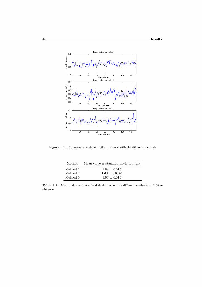
48 Results
Figure 8.1. 153 measurements at 1.68 m distance with the different methods
Method Mean value ± standard deviation (m)Method 1 1.68 ± 0.015Method 2 1.68 ± 0.0070Method 5 1.67 ± 0.015
Table 8.1. Mean value and standard deviation for the different methods at 1.68 mdistance

8.1 Length estimations 49
Figure 8.2. 151 measurements at 9.90 m distance with the different methods
Method Mean value ± standard deviation (m)Method 1 10.13 ± 0.29Method 2 10.22 ± 0.33Method 5 9.94 ± 0.50
Table 8.2. Mean value and standard deviation for the different methods at 9.90 mdistance
The result gets worse as the distance increases. From Fig. 8.1 each measure-ment differs no more then 4-5 cm but at the distance 9.90 each measurement canvary up to 1.5 m. For long distances this radar does not have sufficient accuracyto be of practical use. For this reason no measuring at greater distances has beenperformed. In Appendix B corresponding plots for more distances are shown.
As discussed in Section 7 the inner length of the hardware is assumed to bea constant offset, in Fig. 8.3 an experiment of this is made. The figure shows 16mean valued measurements using method 5 for different lengths from 1.5 to 9.9m, each length is marked with a star in the figure and the straight line is a leastsquare approximation. If the offset is to be just an offset and not a difference

50 Results
in slope all individual measurements should lie in the direct neighborhood of theline. The straight line has a slope of 1.0037, this means that the radar drifts 3.7mm for every meter. In Fig. B.4 in Appendix B the corresponding data for the
Figure 8.3. Each mean value from a measurements are marked with a star and a straightline approximation is made. Method 5 have been used in this plot
other two methods are shown. All three methods seem to follow the straight lineswell, the slopes for method 1 and method 2 are 1.0423 and 1.0542 respectively.Because each sample lies closest to the straight line for method 5, see the figuresin Appendix B for method 1 and 2 to compare, method 5 has the best linearbehavior.
8.2 Confidence intervalWith the aid of a confidence interval the mean value of a series of measurementscan be locked in a certain interval with a chosen probability. If the data has anormal distribution no system fault is present and all inaccuracies derive fromother fault sources. In Fig. 8.4 the estimated error from a series of measurementsat 1.5 m is compared to a perfectly normal distributed variable shown as thestraight line in the figure. Each sample follows the line good enough to assumethat the data is normal distributed.
In Fig. 8.5 a series of 162 measurements at 1.50 m is performed and the con-fidence interval is calculated. From Fig. 8.4 the data is known to be normallydistributed and therefore the confidence interval can be obtained. The continuousline is the mean value of all measurements up to the current value, i.e. the lastvalue corresponds to the mean value including all 162 individual measurements.The dotted lines are the 99 percentage interval and the continuous horizontal linesare the goal accuracy. This value is set to±1 mm corresponding to the performanceof some products currently operating the market today. To fulfill the performancegoal the dotted lines should cross the horizontal lines, when this occurs one can

8.2 Confidence interval 51
Figure 8.4. A plot showing the normal distribution property of the estimated error
with 99 percent certainty know that the result lies inside the goal interval. Fromthe figure it seems this is not the case unfortunately. For this relatively shortdistance the result is however not far from the goal compared to greater distances.In the figure method 5 has been used for length estimation and in Appendix B thesame kind of plot is shown for methods 1 and 2 and also for more distances.
Figure 8.5. Confidence interval for a 162 long series of measurements at 1.5 m distance.The continuous line is the mean value, the dots are the individual measurements, thedotted lines are the confidence interval and the horizontal lines are the goal performance.
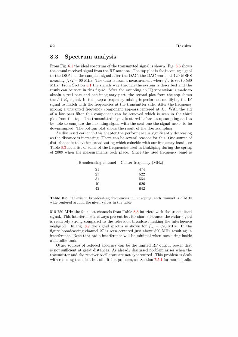
52 Results
8.3 Spectrum analysisFrom Fig. 6.1 the ideal spectrum of the transmitted signal is shown. Fig. 8.6 showsthe actual received signal from the RF antenna. The top plot is the incoming signalto the DSP i.e. the sampled signal after the DAC, the DAC works at 120 MSPSmeaning fs/2 = 60 MHz. The data is from a measurement where ftx is set to 580MHz. From Section 5.1 the signals way through the system is described and theresult can be seen in this figure. After the sampling an IQ separation is made toobtain a real part and one imaginary part, the second plot from the top showsthe I + iQ signal. In this step a frequency mixing is performed modifying the IFsignal to match with the frequencies at the transmitter side. After the frequencymixing a unwanted frequency component appears centered at fs. With the aidof a low pass filter this component can be removed which is seen in the thirdplot from the top. The transmitted signal is stored before its upsampling and tobe able to compare the incoming signal with the sent one the signal needs to bedownsampled. The bottom plot shows the result of the downsampling.
As discussed earlier in this chapter the performance is significantly decreasingas the distance is increasing. There can be several reasons for this. One source ofdisturbance is television broadcasting which coincide with our frequency band, seeTable 8.3 for a list of some of the frequencies used in Linköping during the springof 2009 when the measurements took place. Since the used frequency band is
Broadcasting channel Center frequency (MHz)21 47427 52231 55440 62642 642
Table 8.3. Television broadcasting frequencies in Linköping, each channel is 8 MHzwide centered around the given values in the table.
510-750 MHz the four last channels from Table 8.3 interfere with the transmittedsignal. This interference is always present but for short distances the radar signalis relatively strong compared to the television broadcast making the interferencenegligible. In Fig. 8.7 the signal spectra is shown for ftx = 520 MHz. In thefigure broadcasting channel 27 is seen centered just above 520 MHz resulting ininterference. Note that radio interference will be minimal when measuring insidea metallic tank.
Other sources of reduced accuracy can be the limited RF output power thatis not sufficient at great distances. As already discussed problem arises when thetransmitter and the receiver oscillators are not syncronized. This problem is dealtwith reducing the effect but still it is a problem, see Section 7.5.1 for more details.

8.3 Spectrum analysis 53
Figure 8.6. Received signal from the antenna when ftx = 580 MHz. The top plot showsthe sampled signal, the second is after IQ separation and frequency mixing, the third isafter low pass filtering the unwanted frequency component obtained from the frequencymixing. The last plot shows the signal after downsampling.

54 Results
Figure 8.7. Received signal from the antenna when ftx = 520 MHz. The top plot showsthe sampled signal, the second is after IQ separation and frequency mixing, the third isafter low pass filtering the unwanted frequency component obtained from the frequencymixing. The last plot shows the signal after downsampling. For great distances thedisturbance from the TV broadcasting is significant.
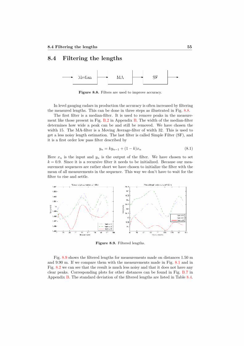
8.4 Filtering the lengths 55
8.4 Filtering the lengths
Figure 8.8. Filters are used to improve accuracy.
In level gauging radars in production the accuracy is often increased by filteringthe measured lengths. This can be done in three steps as illustrated in Fig. 8.8.
The first filter is a median-filter. It is used to remove peaks in the measure-ment like those present in Fig. B.2 in Appendix B. The width of the median-filterdetermines how wide a peak can be and still be removed. We have chosen thewidth 15. The MA-filter is a Moving Average-filter of width 32. This is used toget a less noisy length estimation. The last filter is called Simple Filter (SF), andit is a first order low pass filter described by
yn = kyn−1 + (1− k)xn (8.1)
Here xn is the input and yn is the output of the filter. We have chosen to setk = 0.9. Since it is a recursive filter it needs to be initialized. Because our mea-surement sequences are rather short we have chosen to initialize the filter with themean of all measurements in the sequence. This way we don’t have to wait for thefilter to rise and settle.
Figure 8.9. Filtered lengths.
Fig. 8.9 shows the filtered lengths for measurements made on distances 1.50 mand 9.90 m. If we compare them with the measurements made in Fig. 8.1 and inFig. 8.2 we can see that the result is much less noisy and that it does not have anyclear peaks. Corresponding plots for other distances can be found in Fig. B.7 inAppendix B. The standard deviation of the filtered lengths are listed in Table 8.4.
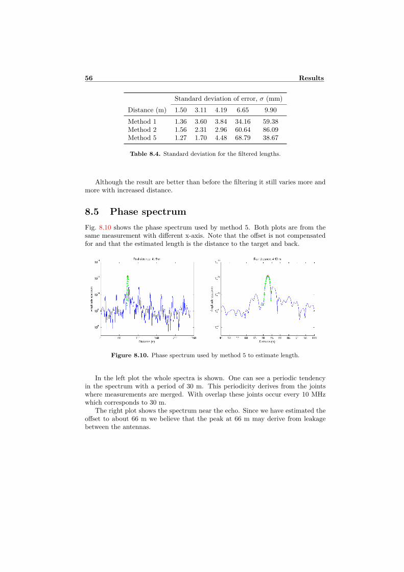
56 Results
Standard deviation of error, σ (mm)Distance (m) 1.50 3.11 4.19 6.65 9.90Method 1 1.36 3.60 3.84 34.16 59.38Method 2 1.56 2.31 2.96 60.64 86.09Method 5 1.27 1.70 4.48 68.79 38.67
Table 8.4. Standard deviation for the filtered lengths.
Although the result are better than before the filtering it still varies more andmore with increased distance.
8.5 Phase spectrumFig. 8.10 shows the phase spectrum used by method 5. Both plots are from thesame measurement with different x-axis. Note that the offset is not compensatedfor and that the estimated length is the distance to the target and back.
Figure 8.10. Phase spectrum used by method 5 to estimate length.
In the left plot the whole spectra is shown. One can see a periodic tendencyin the spectrum with a period of 30 m. This periodicity derives from the jointswhere measurements are merged. With overlap these joints occur every 10 MHzwhich corresponds to 30 m.
The right plot shows the spectrum near the echo. Since we have estimated theoffset to about 66 m we believe that the peak at 66 m may derive from leakagebetween the antennas.
Chapter 9
Closure
9.1 ConclusionsIn this master thesis project we have studied the possibility to measure distanceusing an OFDM-modulated signal. This is desired because, since OFDM is widelyused in radio communication, cheap components are available on the market andusing off-the-shelf components will reduce production costs of level gauging radarssignificantly.
We had two main goals with this project and we consider them both to be ful-filled. We have found that OFDM-modulation can be used to measure distance.This has been confirmed with simulations in MatLab as well as with experimen-tal measurements using the test rig described in Section 5.3. Even though muchtime and energy have been spent trying to increase the performance of the lengthestimation, the accuracy is somewhat lower than we hoped. As discussed in Chap-ter 8 we get pretty good accuracy at short distances, 1-3 m, but the performancedecreases as the distance grows.
We believe that the deteriorated performance largely are due to interferencefrom television broadcastings, as is discussed in Section 8.3. This interference isnext to impossible to counter without changing frequency.
The random offset, ξ, on the phase is another source of disturbance. But sincewe use overlapping measurements we believe ξ’s influence to be minimal.
Although the accuracy of our measurements is not what we had hoped webelieve that if a suitable hardware platform is found an OFDM-modulated signalcould be used to measure distances with high precision.
9.2 Further workTo deeper investigate the possibility to achieve high accuracy at low cost thisproject can be further developed. An RF module using one oscillator for boththe transmitter and receiver results in constant phase difference between measure-ments. This will improve method 5 but also enable the use of methods 3 and 4,
57
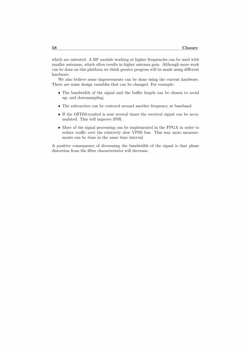
58 Closure
which are untested. A RF module working at higher frequencies can be used withsmaller antennas, which often results in higher antenna gain. Although more workcan be done on this platform we think greater progress will be made using differenthardware.
We also believe some improvements can be done using the current hardware.There are some design variables that can be changed. For example:
• The bandwidth of the signal and the buffer length can be chosen to avoidup- and downsampling.
• The subcarriers can be centered around another frequency at baseband.
• If the OFDM-symbol is sent several times the received signal can be accu-mulated. This will improve SNR.
• More of the signal processing can be implemented in the FPGA in order toreduce traffic over the relatively slow VPSS bus. This way more measure-ments can be done in the same time interval.
A positive consequence of decreasing the bandwidth of the signal is that phasedistortion from the filter characteristics will decrease.

Bibliography
[1] Peter Devine. radar level measurement, the user’s guide. VEGA Controls Ltd,2000. ISBN 0-9538920-0-X.
[2] ELFA. Antenn x-line gold 40xd, uhf. http://www1.elfa.se/elfa~se_sv/go.jsp?s=se-sv&i=78-252-92, May 2009.
[3] Fredrik Gustafsson, Lennart Ljung, and Mille Millnert. Signalbehandling. Stu-dentlitteratur, 2nd edition, 2000. ISBN 978-91-44-01709-9.
[4] Lyrtech Inc. SFF SDR Development Platform User’s guide version 1.1, October2007.
[5] Mohinder Jankiraman. Space-time codes and MIMO systems. Artech House,Inc, 2004. ISBN 1-58053-865-7.
[6] Lennart Råde and Bertil Westergren. Mathematics Handbook for science andengineering. Studentlitteratur, 5th edition, 2004. ISBN 91-44-03109-2.
[7] Sune Söderkvist and Lars-Erik Ahnell. Tidsdiskreta Signaler & System.Söderkvist, Sune, 3rd edition, 2005.
[8] Merrill I. Skolnik. Radar Handbook. McGraw-Hill Professional, New York,NY, 2nd edition, 1990. ISBN 0-07-057913-X.
[9] Merrill I. Skolnik. Introduction to Radar systems. McGraw-Hill Professional,New York, NY, 3 edition, 2001. ISBN 0-07-288138-0.
59


Nomenclature
ADC Analog to Digital Converter
CW Continuous Wave
DAC Digital to Analog Converter
DSP Digital Signal Processor
FFT Fast Fourier Transform
FMCW Frequency Modulated Continuous Wave
FPGA Field-Programmable Gate Array
GPP General-Purpose Processor
ICI Inter Carrier Interference
IF Imtermediate Frequency
IFFT Inverse Fast Fourier Transform
ISI Inter Symbol Interference
LP Low Pass
MA Moving Average
MFCW Multiple Frequency Continuous Wave
MSPS Mega Sample Per Second
MTI Moving Target Indication
OFDM Orthogonal Frequency-Division Multiplexing
PLL Phase Locked Loop
PRBS Pseudo-Random Binary Sequence
QPSK Quadrature Phase Shift Keying
Radar RAdio Detection And Ranging
61

62 Bibliography
RAM Random Access Memory
RF Radio Frequency
SDR Software Defined Radio
SF Simple Filter
SFF Small Form Factor
SNR Signal to Noise Ratio
SoC System on Chip
VPSS Video Processing SubSystem

Appendix A
Flowcharts
63

64 Flowcharts
Figure A.1. Flowchart of program running in the FPGA

65
Figure A.2. Flowchart of the main system in the DSP

66 Flowcharts
Figure A.3. Flowchart of the inner loop seen in the main flowchart

Appendix B
Result plots
67

68 Result plots
Figure B.1. A series of measurements on 3.11 m distance with the different methods
Method Mean value ± standard deviation (m)Method 1 3.18 ± 0.016Method 2 3.18 ± 0.0083Method 5 3.15 ± 0.013
Table B.1. Mean value and standard deviation for the different methods at 3.11 mdistance
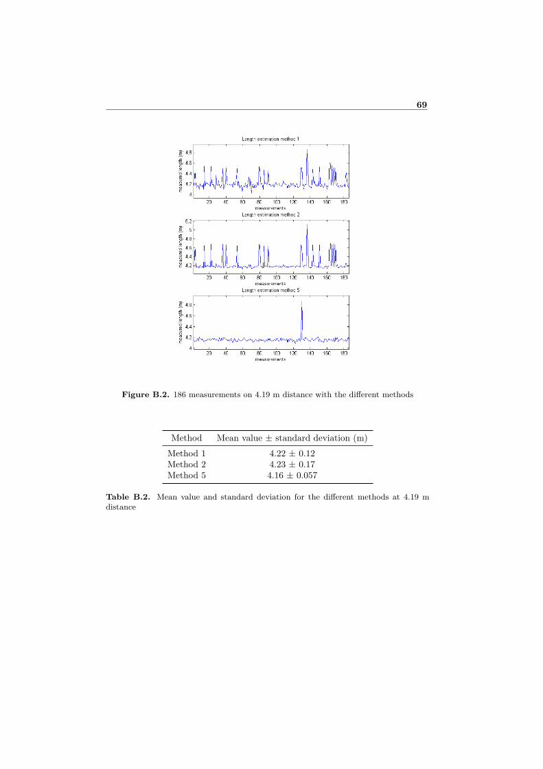
69
Figure B.2. 186 measurements on 4.19 m distance with the different methods
Method Mean value ± standard deviation (m)Method 1 4.22 ± 0.12Method 2 4.23 ± 0.17Method 5 4.16 ± 0.057
Table B.2. Mean value and standard deviation for the different methods at 4.19 mdistance

70 Result plots
Figure B.3. A series of measurements on 6.65 m distance with the different methods
Method Mean value ± standard deviation (m)Method 1 6.89 ± 0.35Method 2 6.96 ± 0.43Method 5 6.69 ± 0.46
Table B.3. Mean value and standard deviation for the different methods at 6.65 mdistance
71
Figure B.4. Linear behavior for method 1 and 2
Figure B.5. Confidence interval using length estimation method 5 for different lengths,to the left 3.565 m is measured and to the right 9.90 m
Figure B.6. Confidence interval at a distance of 1.50 m. The left plot uses method 1for length estimation and the right uses method 2.

72 Result plots
Figure B.7. Filtered lengths.

UpphovsrättDetta dokument hålls tillgängligt på Internet — eller dess framtida ersättare —under 25 år från publiceringsdatum under förutsättning att inga extraordinäraomständigheter uppstår.
Tillgång till dokumentet innebär tillstånd för var och en att läsa, ladda ner,skriva ut enstaka kopior för enskilt bruk och att använda det oförändrat för icke-kommersiell forskning och för undervisning. Överföring av upphovsrätten vid ensenare tidpunkt kan inte upphäva detta tillstånd. All annan användning av doku-mentet kräver upphovsmannens medgivande. För att garantera äktheten, säker-heten och tillgängligheten finns det lösningar av teknisk och administrativ art.
Upphovsmannens ideella rätt innefattar rätt att bli nämnd som upphovsmani den omfattning som god sed kräver vid användning av dokumentet på ovan be-skrivna sätt samt skydd mot att dokumentet ändras eller presenteras i sådan formeller i sådant sammanhang som är kränkande för upphovsmannens litterära ellerkonstnärliga anseende eller egenart.
För ytterligare information om Linköping University Electronic Press se för-lagets hemsida http://www.ep.liu.se/
CopyrightThe publishers will keep this document online on the Internet — or its possi-ble replacement — for a period of 25 years from the date of publication barringexceptional circumstances.
The online availability of the document implies a permanent permission foranyone to read, to download, to print out single copies for his/her own use andto use it unchanged for any non-commercial research and educational purpose.Subsequent transfers of copyright cannot revoke this permission. All other uses ofthe document are conditional on the consent of the copyright owner. The publisherhas taken technical and administrative measures to assure authenticity, securityand accessibility.
According to intellectual property law the author has the right to be mentionedwhen his/her work is accessed as described above and to be protected againstinfringement.
For additional information about the Linköping University Electronic Pressand its procedures for publication and for assurance of document integrity, pleaserefer to its www home page: http://www.ep.liu.se/
c© Jimmy KarlssonOskar Larsson