Screening Overconfident Consumers∗

Michael D. Grubb

Graduate School of Business

Stanford University

Stanford, CA 94305

mgrubb@stanford.edu

www.stanford.edu/~mgrubb

December 10, 2005

Abstract

Consumers may overestimate the precision of their demand forecasts. This overconfidence

creates an incentive for both monopolists and competitive firms to offer tariffs with included

quantities at zero marginal cost, followed by steep marginal charges. This matches observed cell-

phone service pricing plans in the US and elsewhere. An alternative explanation with common

priors can be ruled out in favor of overconfidence based on observed customer usage patterns

for a major US cellular phone service provider. The model can be reinterpreted to explain the

use of flat rates and late fees in rental markets, and teaser rates on loans. Nevertheless, firms

may benefit from consumers losing their overconfidence.

∗I am very grateful to Jeremy Bulow and Jonathan Levin for many valuable discussions of the issues in the paperand to Katja Seim for help and advice especially in obtaining data. For helpful comments and suggestions, I wouldalso like to thank Susan Athey, Lawrence Ausubel, Doug Bernheim, Simon Board, Carlos Corona, Liran Einav, ErikEyster, David Laibson, Edward Lazear, Peter Lorentzen, Muriel Niederle, Peter Reiss, John Roberts, Illya Segal,Enrique Seira, Andrzej Skrzypacz, and Steven Tadelis.

1 Introduction

US cellular phone service providers typically offer consumers a menu of three-part tariffs. Each

tariff consists of a fixed fee F , an included number of minutes Q for which marginal price is zero,

and a positive marginal price p (or overage rate) for minutes beyond Q. Figure 1 below depicts an

example of such a menu taken from Verizon’s website on February 24th 2004.

Verizon "America's Choice" Tariffs

$0$50

$100$150$200$250$300$350

0 1000 2000 3000 4000 5000 6000

(Peak-Time) Minutes Used

Bill

Figure 1: Verizon’s menu of "America’s Choice" tariffs as advertised on their website on February24th 2004. (America’s Choice tariffs are national rather than regional plans.)

The existing literature on non-linear pricing does not provide a compelling explanation for

such pricing patterns. Instead, a tendency of consumers to underestimate the variance of their

future demand when choosing a tariff provides a more plausible explanation of observed menus of

three-part tariffs. Two important biases lead to this tendency: forecasting overconfidence, which

has been well documented in the psychology literature, and projection bias, which is described by

Loewenstein, O’Donoghue and Rabin (2003).

Loewenstein et al. (2003) present a variety of evidence demonstrating the prevalence of projec-

tion bias. Individuals who exhibit this bias overestimate the degree to which their future tastes

will resemble their current tastes, and therefore tend to underestimate the variance of their future

demand. Moreover, a significant body of literature shows that individuals are overconfident about

the precision of their own predictions when making difficult1 forecasts. In other words, individuals

tend to set overly narrow confidence intervals relative to their own confidence levels.

1Predicting one’s future demand for minutes is a relatively difficult task, at least for new cell-phone users. Con-sumers must predict not only the volume of outgoing calls they will make, but also the number of incoming calls theywill receive.

1

Lichtenstein, Fischhoff and Phillips (1982) and Arkes (2001) provide surveys of the experimental

literature concerning forecasting overconfidence. A typical study in this literature might pose the

following question to a group of subjects: "What is the shortest distance between England and

Australia?" Subjects would then be asked to give a set of confidence intervals centered on the

median. Lichtenstein et al. (1982) tabulate the results of 13 such studies. A typical finding is

that the true answer lies outside a subject’s 98% confidence interval about 30% to 40% of the

time. The literature provides evidence that overconfidence diminishes with appropriate feedback

(Bolger and Onkal-Atay 2004), but also that professionals are often overconfident within the realms

of their expertise (Griffin and Tversky 1992). Experimental evidence therefore suggests that, at

a minimum, new cell-phone users will be overconfident about their usage predictions when they

initiate service and choose a calling tariff. Moreover, ex post tariff-choice "mistakes" made by

cellular phone customers are consistent with such overconfidence, as documented in Section 7.

Intuitively, underestimating variance of future demand may lead to tariffs of the form observed

because consumers do not take into account the risk inherent in the convexity of the tariffs on the

menu. This is because although the tariffs have a high average cost per minute for consumers who

consume far above or far below their included minutes, consumers are overly certain that they will

choose a tariff with a number of included minutes that closely matches their consumption. Thus

they expect to pay a low average price per minute. Sellers are then able to profit ex post when

consumers make large revisions in either direction, without having to give up anything ex ante.

This intuition is illustrated with a simple example in Section 2.

In order to make this argument rigorous and focus on the role of overconfidence, I make one

major modeling simplification. I abstract from the initial screening between tariffs, and assume that

consumers have homogenous priors ex ante. In this case, firms optimally offer only a single tariff.

In other words, I focus on explaining why one of Verizon’s offered tariffs would be a three-part

tariff independent of other tariffs on the menu. This assumption is relaxed in Section 8.1.

With one "type" of consumer ex ante, if there is no overconfidence then firms will charge a

fixed fee and set marginal price equal to marginal cost under both monopoly and perfect compe-

tition. Pricing, however, becomes qualitatively different when consumers are overconfident. Given

consumer overconfidence, free disposal of cell-phone minutes, and low marginal costs, I show in

Section 4 that under either monopoly or perfect competition, consumers will be offered a tariff

which involves a range of minutes offered at zero marginal price, followed by positive marginal

prices for further minutes. This provides a plausible explanation for the form of cell phone tariffs

observed in the US. I develop further intuition for the result, based on option pricing, in Section 5.

My earlier assertion that consumer overconfidence and projection bias provide a better expla-

2

nation of observed menus of three-part tariffs than do existing models of non-linear pricing deserves

further explanation. Any model which explains the use of three-part tariffs should capture their

primary qualitative feature: included quantities at zero marginal price followed by positive mar-

ginal charges. Moreover, any model which explains cellular phone service pricing must also be

consistent with two additional stylized facts concerning usage. These are based on an analysis of

billing records for 2,332 customers of a national US cellular phone service provider over a 41 month

period (Section 7).

First, overages are an important feature of customer behavior and an important source of firm

revenue. On tariffs with positive included minutes, consumers make overages on 19% of bills,

thereby generating 23% of revenues. Second, customers on plans with more included minutes use

more minutes. Specifically, the distribution of usage by customers on a plan with a large number

of included minutes strictly first order stochastically dominates (FOSD) the distribution of usage

by customers on a plan with a small number of included minutes.

Now consider the monopoly model of non-linear pricing developed by Mussa and Rosen (1978).

The model assumes buyers do not to learn more information about their demand over time, and

thus views the decision to participate in an offered tariff and the decision about how much to

consume as simultaneous. Within this framework, a menu of two-part tariffs, each consisting of a

fixed fee F and a marginal price p, can be thought of as a useful way to implement a single concave

non-linear tariff. It does not explain, however, the need for three-part tariffs.2

Of course while standard screening models are static, reality is dynamic. Consumers first choose

from a menu of offered tariffs, and then later choose how much to consume. In the intervening

period, consumers may acquire more private information about their demand. The most natural

alternative to the model presented in this paper is therefore an extension of Courty and Li’s (2000)

model of sequential screening. As discussed in Section 6, under certain conditions this extension does

predict that a monopolist will offer a menu of tariffs with initial minutes included at zero marginal

price. However, this prediction only holds under assumptions which generate consumption patterns

inconsistent with those documented in Section 7.

For instance, under assumptions which generate tariffs similar to those offered by Verizon, the

extension of Courty and Li’s (2000) model would predict that consumers who chose a 2500 minute

2Of course, prices on a particular tariff for quantities that are never chosen may be somewhat arbitrary. In a staticscreening model, all that matters in a tariff menu is the lower envelope of tariffs on the menu. Segments of tariffswhich are above that minimum may be set arbitrarily, for instance to include regions of zero marginal price.This does not explain the structure of cell phone tariffs, however. First, Figure 1 shows that zero marginal price

regions are part of the lower envelope of tariffs on the menu. What is more, customer billing data shows that usagefalls within the zero marginal price regions of tariffs approximately 80% of the time, and then on average reachesonly half of the included allowance.

3

plan would be weakly more likely to consume fewer than 500 minutes than consumers who chose the

500 minute plan. This is inconsistent with the observed FOSD ordering of consumption patterns

across plans. Moreover, the result collapses entirely under perfect competition. In contrast, the

model presented in this paper not only predicts observed pricing patterns under both monopoly

and perfect competition, but is also consistent with both stylized facts concerning usage patterns.

The model of screening overconfident consumers is also applicable beyond cellular phone mar-

kets. In particular, it may explain a variety of tariffs where late fees are charged if the quantity

variable is interpreted as time. For instance rental car companies often charge a flat rate for a

one-week rental, but begin charging by the hour once the car is returned late. Similar late fees are

used in other rental markets such as video rentals.3

The model may also explain the prevalence of introductory interest rate offers by credit card

companies, by again interpreting quantity as time. One explanation for increasing interest rates

is simply that the marginal cost increases because consumers who demand longer loan times are

riskier. This work shows, however, that an alternate explanation is that consumers are overconfident

when they predict how long they will need the loan - and overestimate the likelihood of paying

back the loan near to the expiry of the introductory rate.

Given the model and analysis developed in Sections 3-4 it is simple to consider the reverse case in

which consumers are underconfident and overestimate the variance of their future demand. Psychol-

ogy literature documents the hard-easy effect:4 While individuals are overconfident when making

difficult predictions, they are actually underconfident when making simple predictions (Lichtenstein

et al. 1982). In this case equilibrium pricing involves marginal prices that are above marginal cost

at low quantities, but fall below marginal cost, perhaps all the way to zero, at high quantities. This

pricing is qualitatively similar to that found in a standard model of quantity discounts (Mussa and

Rosen 1978), although with steeper discounts in the sense that marginal prices fall below marginal

costs. While there are already explanations in the literature (see Hartmann and Viard (2005) for an

overview), this paper provides an alternative explanation for why we observe loyalty programs such

as "play ten rounds of golf - get one free," which implement quantity discounts without committing

consumers to a purchase quantity in advance. More empirical work is needed to determine which

explanations are important.

3Blockbuster announced the "end of late fees" in 2005, but customers are charged a restocking fee of $1.25 formovies over 7 days late and the full retail price of movies over 37 days late (Koenig 2004).

4 It should be noted that the hard-easy effect has been documented for binary predictions such as, "Is London orSydney more populous?" rather than continuous predictions such as "How far is it between London and Sydney?"which are relevant here. Moreover, some authors have called into question the validity of results documenting thehard-easy effect for such binary predictions (Juslin, Winman and Olsson 2000).

4

2 Illustrative Example

At this point a simple example may be useful to illustrate the main results explored in this paper,

and clarify the intuition behind them. Assume that a supplier has a constant marginal cost of 5

cents per minute and a fixed cost of $50 per customer.5 Consider the case in which consumers value

each additional minute of consumption at 45 cents up to some satiation point, beyond which they

value further minutes at 0 cents.

Further, assume that when consumers sign up for a tariff in period one, they are homogeneously

uncertain about their satiation points. Then in period two, consumers learn their satiation points,

and use this information to make their consumption choices. In particular, assume that one third

of consumers learn that they will be satiated after 100 minutes, one third after 400 minutes, and

the remaining third after 700 minutes.

If consumers and the supplier share this prior belief, then it is optimal for the firm to charge

a marginal price equal to the marginal cost of 5 cents per minute.6 Under monopoly the firm

extracts all the surplus via a fixed fee of $160, earning profits of $110 per customer. Under perfect

competition, the firm charges a fixed fee of $50, leaving $110 in surplus to consumers.

If consumers are overconfident, however, marginal cost pricing is no longer optimal. For instance,

if all consumers are extremely overconfident and believe that they will be satiated after 400 minutes

with probability one, then it is optimal to charge 0 cents per minute for the first 400 minutes, and

45 cents per minute thereafter. In other words it is optimal to have 400 "included" minutes in the

tariff.

Under monopoly the firm charges a fixed fee of $180, earning expected profits of $155 per

customer. Ex ante consumers expect to receive zero surplus, but on average ex post realize a loss

of $45. Under perfect competition, the firm charges a fixed fee of $25, and consumers expect to

receive $155 in surplus, but actually only realize $110. The consumers’ overconfidence allows the

creation ex ante of an additional $45 in perceived consumer surplus, which is never realized ex post.

To see why this tariff is optimal, consider the pricing of minutes 100-400 and 400-700 separately.

On the one hand, overconfident consumers believe that they will consume minutes 100-400 with

probability 1, while the firm knows that they will actually consume them only with probability 23 .

As a result, reducing the marginal price of minutes 100-400 from 5 cents to 0 cents is perceived

5Fixed costs per customer may arise due to billing costs, a subsidy for a new phone, or customer acquisition feespaid to retailers.

6Note that this is only one of a continuum of optimal pricing structures which all implement the efficient allocation.Were demand curves not rectangular and were there a continuum of types, then marginal cost pricing would beuniquely optimal.

5

differently by the firm and consumer. The consumer views this as a $15 price cut and will be

indifferent if the fixed fee is increased by $15. The firm, however, recognizes this as only a $10

revenue loss, and will be better off by $5 if the fixed fee is raised by $15.

On the other hand, overconfident consumers believe that they will consume minutes 400-700

with probability 0, while the firm knows that they will actually consume them with probability 13 .

Therefore from the consumer’s perspective, increasing the marginal price of minutes 400-700 from

5 cents to 45 cents does not impact the expected price paid. The firm, however, views this as an

increase in expected revenues of $40.

Essentially, the firm finds it optimal to sell the first 400 minutes upfront to the overconfident

consumer. Then in the second period, the firm buys back minutes 100-300 from the low demand

consumers at the monopsony price of 0 cents per minute, and sells minutes 400-700 to high demand

consumers at the monopoly price of 45 cents per minute.

Note that in this example, a monopolist earns higher profits from overconfident consumers,

making them worse off than consumers with correct priors. Under competition, however, overcon-

fident consumers are equally as well off as consumers with correct priors. Neither result is true in

general, rather both follow from the specific form of preferences assumed (see Section 4.6).

3 Model Outline

The base assumptions about production and preferences match those of a standard screening model.

A firm’s profits Π (q, P ) are given by revenues P less production costs C (q), which are increasing

and convex in quantity q. Consumers’ utility U (q, θ, P ) is equal to their value of consumption

V (q, θ) less their payment to the firm, P .

Consumers’ marginal value of consumption Vq is strictly decreasing in consumption q, and

strictly increasing in consumers’ type θ, which parameterizes their level of demand. The outside

option of all consumers is the same and normalized to zero: V (0, θ) = 0. The partial derivative Vqqθ

is assumed to be equal to zero, which is stricter than the standard assumption Vqqθ ≤ 0. With thisadditional assumption it is then without further loss of generality to set Vqθθ = 0 by appropriate

normalization of θ. The consumers’ value function may then be written as V (q, θ) = v (q) + qθ.

I make an additional assumption concerning consumer preferences, which would not be relevant

in a standard model: Consumers have a finite satiation point, qS (θ) ≡ argmaxq≥0 V (q, θ), beyondwhich they may freely dispose of unwanted units.7

7This is equivalent to assuming that beyond their satiation point consumers have zero marginal value ofconsumption.

6

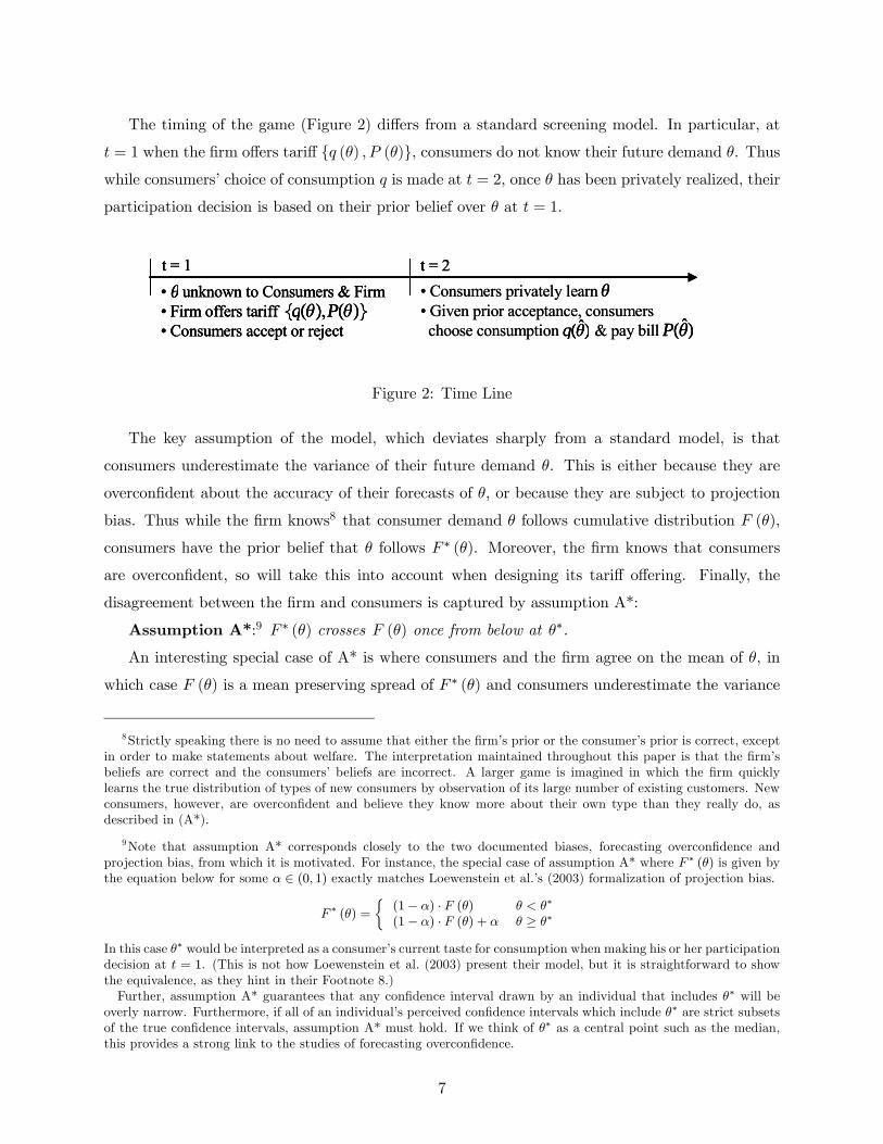
The timing of the game (Figure 2) differs from a standard screening model. In particular, at

t = 1 when the firm offers tariff {q (θ) , P (θ)}, consumers do not know their future demand θ. Thuswhile consumers’ choice of consumption q is made at t = 2, once θ has been privately realized, their

participation decision is based on their prior belief over θ at t = 1.

• Consumers privately learn • Given prior acceptance, consumers choose consumption & pay bill

t = 1 t = 2• unknown to Consumers & Firm• Firm offers tariff • Consumers accept or reject

q,Pq P

• Consumers privately learn • Given prior acceptance, consumers choose consumption & pay bill

t = 1 t = 2• unknown to Consumers & Firm• Firm offers tariff • Consumers accept or reject

q,Pq P

t = 1 t = 2• unknown to Consumers & Firm• Firm offers tariff • Consumers accept or reject

q,Pq P

Figure 2: Time Line

The key assumption of the model, which deviates sharply from a standard model, is that

consumers underestimate the variance of their future demand θ. This is either because they are

overconfident about the accuracy of their forecasts of θ, or because they are subject to projection

bias. Thus while the firm knows8 that consumer demand θ follows cumulative distribution F (θ),

consumers have the prior belief that θ follows F ∗ (θ). Moreover, the firm knows that consumers

are overconfident, so will take this into account when designing its tariff offering. Finally, the

disagreement between the firm and consumers is captured by assumption A*:

Assumption A*:9 F ∗ (θ) crosses F (θ) once from below at θ∗.

An interesting special case of A* is where consumers and the firm agree on the mean of θ, in

which case F (θ) is a mean preserving spread of F ∗ (θ) and consumers underestimate the variance

8Strictly speaking there is no need to assume that either the firm’s prior or the consumer’s prior is correct, exceptin order to make statements about welfare. The interpretation maintained throughout this paper is that the firm’sbeliefs are correct and the consumers’ beliefs are incorrect. A larger game is imagined in which the firm quicklylearns the true distribution of types of new consumers by observation of its large number of existing customers. Newconsumers, however, are overconfident and believe they know more about their own type than they really do, asdescribed in (A*).

9Note that assumption A* corresponds closely to the two documented biases, forecasting overconfidence andprojection bias, from which it is motivated. For instance, the special case of assumption A* where F ∗ (θ) is given bythe equation below for some α ∈ (0, 1) exactly matches Loewenstein et al.’s (2003) formalization of projection bias.

F ∗ (θ) =

½(1− α) · F (θ) θ < θ∗

(1− α) · F (θ) + α θ ≥ θ∗

In this case θ∗ would be interpreted as a consumer’s current taste for consumption when making his or her participationdecision at t = 1. (This is not how Loewenstein et al. (2003) present their model, but it is straightforward to showthe equivalence, as they hint in their Footnote 8.)Further, assumption A* guarantees that any confidence interval drawn by an individual that includes θ∗ will be

overly narrow. Furthermore, if all of an individual’s perceived confidence intervals which include θ∗ are strict subsetsof the true confidence intervals, assumption A* must hold. If we think of θ∗ as a central point such as the median,this provides a strong link to the studies of forecasting overconfidence.

7

of their future demand. Moreover, it implies that consumers correctly predict their mean value of

each minute.

Within the context of this model, the equilibrium tariff, or allocation and payment pair {q∗ (θ) , P ∗ (θ)},will be characterized under both monopoly and perfect competition. This analysis requires several

more technical assumptions. As is standard, it is assumed that V (q, θ) is thrice continuously dif-

ferentiable, C (q) and F (θ) are twice continuously differentiable, F ∗ (θ) is continuous and piecewise

smooth, consumption is non-negative, and total surplus is initially strictly positive. The firm’s prior

F (θ) has full support over£θ, θ¤, a range which includes the support of consumers’ prior F ∗ (θ).

4 Equilibrium Analysis

4.1 Defining the Problem

Invoking the standard revelation principle, the equilibrium monopoly tariff©qM (θ) , PM (θ)

ªmust

solve the following constrained profit maximization problem:

maxP (θ)q(θ)≥0

E [Π (θ)]

such that

Global IC U (θ, θ) ≥ U(θ, θ) ∀θ, θ ∈£θ, θ¤

Consumer Participation10 E∗ [U (θ)] ≥ 0Free Disposal q (θ) ≤ qS (θ)

The monopolist’s problem in this case is similar to that of a standard screening problem. The

monopolist’s objective is the same: to maximize expected profits E [Π (θ)], where Π (θ) ≡ P (θ) −C (q (θ)) denotes the firm’s profit from serving a consumer who reports type θ. Moreover, at time

t = 2 when consumers privately learn their types, it must be optimal for consumers to truthfully

reveal their types by self-selecting appropriate quantity - payment pairs from the tariff. Thus the

standard incentive compatibility constraint applies: the utility U³θ, θ´≡ V

³q³θ´, θ´−P

³θ´of

a consumer of type θ who reports θ at t = 2 must be weakly below the utility U (θ) ≡ U (θ, θ) of a

consumer of type θ who reports truthfully at t = 2.

10Expectations taken with respect to the consumers’ prior F ∗ (θ) are denoted by a superscript * on the expectationsoperator.

8

The remaining constraints, however, incorporate two important deviations from a standard

screening model. First, the additional constraint of free disposal is explicitly imposed.11 Second,

consumers’ ex ante prior over types F ∗ (θ) differs from that of the firm F (θ). Thus the ex ante

participation constraint requires that consumers’ perceived expected utility E∗ [U (θ)] must be

positive, but puts no constraint on their true expected utility E [U (θ)]. The difference in priors

between consumers and the firm creates a wedge separating the expected utility consumers believe

they are receiving from the expected utility the firm believes it is actually providing.

Invoking the revelation principle a second time, the equilibrium tariff©qC (θ) , PC (θ)

ªunder

perfect competition must solve the following closely related constrained maximization problem:

maxP (θ)q(θ)≥0

E∗ [U (θ)]

such that

Global IC U (θ, θ) ≥ U(θ, θ) ∀θ, θ ∈£θ, θ¤

Producer Participation E [Π (θ)] ≥ 0Free Disposal q (θ) ≤ qS (θ)

As under monopoly, the equilibrium tariff must satisfy free disposal and incentive compatibility

constraints. The difference is that the objective function and participation constraints are re-

versed. Under perfect competition the equilibrium tariff maximizes consumers’ perceived expected

utility subject to firm participation,12 whereas under monopoly firm payoff is maximized subject

to consumer participation.

4.2 Simplifying the Problem

Just as in a standard screening model, the first step, introduced by Mirrlees (1971), is to replace the

global incentive compatibility constraint with the joint constraints of local incentive compatibility

and monotonicity. Both monopoly and perfect competition problems may then be simplified by

substituting local incentive compatibility and participation constraints in place of payments P (θ)

in the objective function.

First define S (θ) ≡ V (q (θ) , θ)−C (q (θ)) as the total surplus achieved from serving a consumerwho truthfully reports type θ. It is straightforward to show that under either monopoly or per-

11This alone would have no impact on a standard monopoly screening model since it would never be binding. Thisassumption will be important here, however, because consumers and the firm have different priors over θ.

12Otherwise there would be an opportunity for profitable entry.

9

fect competition, the relevant participation constraints must bind. This implies that under both

monopoly and perfect competition, the objective function is equal to expected surplus E [S (θ)]

plus a perception gap:

E [S (θ)] +E∗ [U (θ)]−E [U (θ)] (1)

The perception gap E∗ [U (θ)]−E [U (θ)] is the difference between the expected utility E∗ [U (θ)]consumers believe they are receiving and the expected utility E [U (θ)] the firm believes it is de-

livering. When consumers and the firm share the same prior (F ∗ (θ) = F (θ)) the perception

gap is zero, so the equilibrium tariff maximizes expected surplus E [S (θ)]. This implies first best

allocation qFB (θ) and marginal payment equal to marginal cost.

qFB (θ) ≡ argmaxq[V (q, θ)− C (q)]

When consumers are overconfident, however, the perception gap need not be zero, and may distort

the equilibrium allocation away from first best, and marginal pricing away from marginal cost.

Local incentive compatibility requires that U 0 (θ) = Vθ (q (θ) , θ). By applying the fundamental

theorem of calculus (FTC), taking expectations, and integrating by parts, it can be shown that

local incentive compatibility pins down the perception gap as given in equation (2):

E∗ [U (θ)]−E [U (θ)] = E

∙Vθ (q (θ) , θ)

F (θ)− F ∗ (θ)

f (θ)

¸(2)

The objective function under both monopoly and perfect competition is the same and has

now been expressed entirely as a function of the allocation q (θ). The remaining constraints not

already incorporated are also identical across market situations. Thus the equilibrium allocation

q∗ (θ) = qM (θ) = qC (θ) will be identical under monopoly and perfect competition. Further it is

characterized as the solution to a simplified maximization problem as described in Proposition 1.

Finally, equilibrium payments can be calculated as a function of the equilibrium allocation by

applying local incentive compatibility and participation constraints (Proposition 1). Since only

participation constraints differ across market conditions, only equilibrium fixed fees will differ be-

tween monopoly and perfect competition. Marginal pricing, which is pinned down by local incentive

compatibility, will be the same across market conditions.13

13The main results are easily extended to imperfect competition in which firms are differentiated by location andconsumers’ transportation costs d are independent of consumption or type θ. (For example V (q, θ, d) = V (q, θ)−d).Equilibrium allocations and marginal prices would be identical to those in the current model, which maximize expectedvirtual surplus. Firms would compete with each other through the fixed fees, which would drop with the level ofcompetition. (In contrast, distortions of price away from marginal cost in a standard price discrimination modeldisappear with increasing competition (Stole 1995).)

10

Proposition 1 Under both monopoly and perfect competition:

1. Equilibrium allocations are identical, and maximize expected virtual surplus:

q∗ (θ) = arg maxq(θ)∈[0,qS(θ)]

q(θ) non-decreasing

E [Ψ (q (θ) , θ)]

Ψ (q, θ) ≡ V (q, θ)−C (q) + Vθ (q (θ) , θ)F (θ)− F ∗ (θ)

f (θ)(3)

2. Payments differ only by a fixed fee and are given by:

PC (θ) = V (q∗ (θ) , θ)−Z θ

θVθ (q

∗ (z) , z) dz −E [S (q∗ (θ) , θ)]

PM (θ) = PC (θ) +E [Ψ (q∗ (θ) , θ)]

3. At quantities for which there is no pooling, marginal price is given by equation (4) as a

function of the inverse equilibrium allocation θ (q):

dP ∗ (q)

dq= Vq (q, θ (q)) (4)

Proof. Outlined in the text above. For further details see Appendix B.

4.3 Equilibrium Allocation

Further characterization of the equilibrium allocation follows the standard approach. First, the

solution qR (θ) to a relaxed problem (equation 5) that ignores the monotonicity constraint is char-

acterized.

qR (θ) ≡ arg maxq∈[0,qS(θ)]

Ψ (q, θ) (5)

Second, any non-monotonicities in qR (θ) are "ironed out." Implications about pricing can then be

drawn based on the result in Proposition 1 that marginal price is equal to Vq (q, θ (q)).

Proposition 2 1. The relaxed solution qR (θ) is a continuous and piecewise smooth function char-

acterized by the first order condition Ψq (q, θ) = 0 except where satiation or non-negativity con-

straints bind.

2. The equilibrium allocation q∗ (θ) is continuous and piecewise smooth. On any interval over

which the monotonicity constraint is not binding, the equilibrium allocation is equal to the relaxed

allocation: q∗ (θ) = qR (θ).

11

Proof. Part 1: See Appendix B. Part 2: The proof of part 2 is omitted as it closely follows ironing

results for the standard screening model. It follows from the application of standard results in

optimal control theory (Leonard and Long 1992, theorems 6.5.1, 6.5.2, 7.8.1, and 7.9.1) and the

Kuhn-Tucker theorem.

Proposition 2 closely parallels analogous results in standard screening models. The important

point is that the equilibrium allocation q∗ (θ) is continuous and equal to the relaxed allocation

qR (θ) where the monotonicity constraint is not binding. This fact is useful since it implies that

the relaxed solution qR (θ) determines marginal prices (Proposition 3).

When consumers are extremely overconfident, the relaxed solution will violate the monotonicity

constraint (Appendix A Proposition 6). Thus to avoid excluding interesting cases, Appendix A

characterizes an ironed solution (Proposition 4) and provides details of pooling in equilibrium.

4.4 Pricing Implications

Having characterized the equilibrium allocation q∗ (θ), it is now possible to draw implications about

pricing using Proposition 1.

Proposition 3 The equilibrium payment P ∗ (q) = P ∗ (θ (q)) is a continuous and piece-wise smooth

function of quantity. There may be kinks in the payment function where marginal price increases

discontinuously. These kinks occur where the monotonicity constraint binds and an interval of types

"pool" at the same quantity. For quantities at which there is no pooling, marginal price is given by

equation (6):dP ∗ (q)

dq= max

½0, Cq (q) + Vqθ (q, θ (q))

F ∗ (θ (q))− F (θ (q))

f (θ (q))

¾(6)

Proof. See Appendix B.

Since it is assumed that Vqθ is strictly positive and f (θ) is finite, Proposition 3 allows marginal

price to be compared to marginal cost based on the sign of [F ∗ (θ)− F (θ)]. In particular, the sign

of£P ∗q (q)− Cq (q)

¤is equal to the sign of [F ∗ (θ)− F (θ)] except when F ∗ (θ) < F (θ) and marginal

cost is zero, since then marginal price is also zero. This is informative about equilibrium pricing,

since assumption A* dictates the sign of [F ∗ (θ)− F (θ)] above and below θ∗.

Define q, Q, and q to be the equilibrium allocations of types θ, θ∗, and θ respectively:

©q,Q, q

ª≡©q∗ (θ) , q∗ (θ∗) , q∗

¡θ¢ª

Relevant implications of Proposition 3 are then summarized in Corollary 1.

12

Corollary 1 For quantities at which there is no pooling: (1) If marginal cost is zero for all q then:

P ∗q (q) = 0 , q ∈¡q,Q

¢∪©q,Q, q

ªP ∗q (q) > 0 , q ∈ (Q, q)

(2) If marginal cost is strictly positive for all q then:

P ∗q (q) = Cq (q) > 0 , q ∈©q,Q, q

ªCq (q) > P ∗q (q) ≥ 0 , q ∈

¡q,Q

¢P ∗q (q) > Cq (q) > 0 , q ∈ (Q, q)

Proof. Follows directly from Proposition 3, assumption A*, and q∗ (θ) non-decreasing.

Corollary 1 shows that when marginal costs are zero, marginal price will be zero below some

included allowance Q, and positive thereafter. When marginal costs are strictly positive, marginal

price will initially be positive, but will fall below marginal cost and may be zero for some early

range of consumption. The following section illustrates these results with numerical examples.

It is reasonable to assume that the marginal cost of providing an extra minute of call time to a

cell phone customer is small. Therefore, given overconfident consumers, the equilibrium tariff bears

a striking qualitative resemblance to those offered by cell-phone service providers. Both predicted

equilibrium tariffs and observed tariffs involve zero marginal price up to some included minute limit

Q and become positive thereafter.

The primary difference is that beyond the included limit Q, marginal price is constant for

observed tariffs. I conjecture that this simpler pricing structure approximates optimal pricing and

is more practical to implement. The fact that marginal price does not fall to marginal cost at

the top may also be due to binding period-one incentive compatibility constraints relevant to the

un-modeled self-selection among tariffs at time one (see Section 8.1).

The intuition for the result is as follows. If consumers are overly confident that their future

consumption will be near Q minutes, they will underestimate both the probability of extremely low

and extremely high consumption. Thus a firm cannot charge these consumers for extremely high

consumption through a fixed fee ex ante. Instead, the firm must wait until consumers learn their

true values and charge a marginal fee for high consumption above Q. A firm can, however, charge

consumers for low levels of consumption through a fixed fee ex ante. By setting a zero marginal

price, the firm avoids paying a refund to those consumers who are later surprised by a low level of

demand below Q.

13

4.5 Example

The implications of Proposition 3 that are summarized in Corollary 1 are best illustrated with figures

from specific examples. Consider the following example which satisfies the model assumptions

outlined in Section 3.

Example 1 Firms have a fixed cost of $25 and a constant marginal cost of c ≥ 0 per unit: C (q) =25 + q · c. Consumers’ inverse demand function is linear in q and θ. In particular, θ simply shifts

the consumers inverse demand curve up and down (Figure 3):

V (q, θ) =3

2q

∙1 + θ − 1

1000q

¸

Vq (q, θ) =3

2

∙1 + θ − 2

1000q

¸The firm and consumers’ priors are uniform, centered on 0: F : U

£−12 ,

12

¤and F ∗ : U

£−∆2 ,

∆2

¤.

-½ ½0

F*F

θΔ

− Δ2

Δ2q

250 750

$ 0.75

$ 2.25V q q, 1

2

V q q, − 12

Figure 3: Inverse demand curves and priors in example 1.

Consumers and the firm both agree that the mean of θ is equal to 0: E∗ [θ] = E [θ] = 0. The

parameter ∆ ∈ [0, 1] is a measure of consumer overconfidence. For ∆ = 1, consumers are not

overconfident at all, and share the firm’s prior. For ∆ = 0, consumers are extremely overconfident

and believe θ = 0 with probability one (Figure 3).

Satiation and first best allocations are given by:

qS (θ) = 500 (1 + θ)

qFB (θ) = 500 (1 + θ − c)

The equilibrium allocation q∗ (θ) and pricing P ∗ (q) depend on the size of marginal cost c and the

level of overconfidence ∆.

Figure 4 illustrates Corollary 1 given zero marginal costs, using the example described above.

In the top row, plots A and B show total equilibrium payment PC (q) and total cost C (q) versus

14

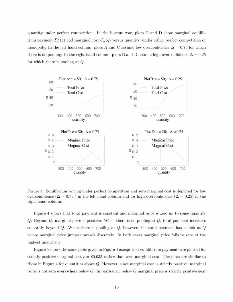
quantity under perfect competition. In the bottom row, plots C and D show marginal equilib-

rium payment P ∗q (q) and marginal cost Cq (q) versus quantity, under either perfect competition or

monopoly. In the left hand column, plots A and C assume low overconfidence ∆ = 0.75 for which

there is no pooling. In the right hand column, plots B and D assume high overconfidence ∆ = 0.25

for which there is pooling at Q.

300 400 500 600 700quantity

00.10.20.30.40.5

$

PlotC: c = $0; D = 0.75

Marginal CostMarginal Price

300 400 500 600 700quantity

00.10.20.30.40.5

$

Plot D: c= $0; D =0.25

Marginal CostMarginal Price

300 400 500 600 700quantity

20

40

60

80

$

Plot A: c = $0; D = 0.75

Total CostTotal Price

300 400 500 600 700quantity

20

40

60

80

$

PlotB: c = $0; D = 0.25

Total CostTotal Price

Figure 4: Equilibrium pricing under perfect competition and zero marginal cost is depicted for lowoverconfidence (∆ = 0.75 ) in the left hand column and for high overconfidence (∆ = 0.25) in theright hand column.

Figure 4 shows that total payment is constant and marginal price is zero up to some quantity

Q. Beyond Q, marginal price is positive. When there is no pooling at Q, total payment increases

smoothly beyond Q. When there is pooling at Q, however, the total payment has a kink at Q

where marginal price jumps upwards discretely. In both cases marginal price falls to zero at the

highest quantity q.

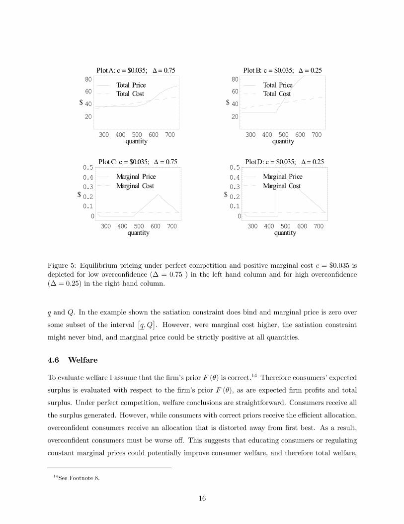
Figure 5 shows the same plots given in Figure 4 except that equilibrium payments are plotted for

strictly positive marginal cost c = $0.035 rather than zero marginal cost. The plots are similar to

those in Figure 4 for quantities above Q. However, since marginal cost is strictly positive, marginal

price is not zero everywhere below Q. In particular, below Q marginal price is strictly positive near

15

300 400 500 600 700quantity

00.10.20.30.40.5

$

Plot C: c = $0.035; D = 0.75

Marginal CostMarginal Price

300 400 500 600 700quantity

00.10.20.30.40.5

$

PlotD: c = $0.035; D= 0.25

Marginal CostMarginal Price

300 400 500 600 700quantity

20

40

60

80

$

PlotA: c = $0.035; D= 0.75

Total CostTotal Price

300 400 500 600 700quantity

20

40

60

80

$

Plot B: c = $0.035; D = 0.25

Total CostTotal Price

Figure 5: Equilibrium pricing under perfect competition and positive marginal cost c = $0.035 isdepicted for low overconfidence (∆ = 0.75 ) in the left hand column and for high overconfidence(∆ = 0.25) in the right hand column.

q and Q. In the example shown the satiation constraint does bind and marginal price is zero over

some subset of the interval£q,Q

¤. However, were marginal cost higher, the satiation constraint

might never bind, and marginal price could be strictly positive at all quantities.

4.6 Welfare

To evaluate welfare I assume that the firm’s prior F (θ) is correct.14 Therefore consumers’ expected

surplus is evaluated with respect to the firm’s prior F (θ), as are expected firm profits and total

surplus. Under perfect competition, welfare conclusions are straightforward. Consumers receive all

the surplus generated. However, while consumers with correct priors receive the efficient allocation,

overconfident consumers receive an allocation that is distorted away from first best. As a result,

overconfident consumers must be worse off. This suggests that educating consumers or regulating

constant marginal prices could potentially improve consumer welfare, and therefore total welfare,

14See Footnote 8.

16

since firm profits are always zero.

Under monopoly, total welfare is also lower when consumers are overconfident, but in general

it is ambiguous as to whether consumers or the firm are better or worse off. The firm earns

expected profits equal to expected virtual surplus, the sum of surplus and the perception gap,

and therefore benefits from consumer overconfidence if and only if this is higher than first best

surplus: E [Ψ∗] ≥ E£SFB

¤. Overconfident consumers’ expected payoff under the correct prior is

the remaining surplus E [S∗]−E [Ψ∗], which is given by the negative of the equilibrium perception

gap. They are therefore worse off if and only if: −EhVθ (q

∗ (θ) , θ) F (θ)−F∗(θ)

f(θ)

i≤ 0. Neither

condition is very helpful since both are in terms of the equilibrium allocation, but Lemma 1 gives

a simple sufficient condition for both to be true.

Lemma 1 Under monopoly, whenever overconfident consumers weakly overestimate the surplus

created by the first best allocation,15 E∗£SFB

¤≥ E

£SFB

¤, the firm is better off and consumers are

worse off due to their overconfidence.

Proof. See Appendix B.

The tables may be turned if overconfident consumers underestimate the expected surplus gener-

ated by the first best allocation, because this under estimation creates bargaining power. The firm

cannot extract all surplus ex ante, and to extract it ex post the firm must give away information

rents since the customer is privately informed about θ in period two. This is the case in the exam-

ples discussed in Section 4.5. There, although it is assumed that consumers estimate the mean of θ

correctly, since the value of first best allocation is proportional to θ2 and overconfident consumers

underestimate the spread of θ, E∗£SFB

¤is strictly below E

£SFB

¤. Moreover, the underestimation

of surplus is great enough that consumers are strictly better off when overconfident. Of course this

also implies that the firm is worse off and would prefer customers to have correct priors.

The discussion of welfare has thus far assumed that consumers are homogeneously overconfident.

If there are both correct-prior and overconfident types served in the marketplace, overconfident

consumers must be weakly worse off than their counterparts with correct priors because correct

beliefs lead to better decisions. That being said, it is possible that the presence of overconfident

types in the marketplace improves the outcome for both types. Since types with correct priors can

always choose any tariff offered to overconfident types, serving overconfident types also limits the

rents which can be extracted from types with correct priors.

15Note that under zero marginal costs, assuming that E∗£SFB

¤≥ E

£SFB

¤is equivalent to assuming that overcon-

fident consumers overestimate their expected value of consuming up to their satiation points.

17

When there is ex ante heterogeneity in average demand (see Section 8.1), overconfidence causes

consumers to believe that they are more different than they really are, and a monopolist must give

up more information rents to screen them. This second effect suggests that consumer overconfidence

is more likely to lower monopoly profits when initial screening of consumers between separate tariffs

is important.

5 Option Pricing Intuition

Consider the case of monopoly. At time one, the monopolist is selling a series of call options, or

equivalently units bundled with put options, rather than units themselves. The marginal price

charged for a unit q at time two is simply the strike price of the option sold on unit q at time one.

The series of call options being sold are interrelated; a call option for unit q can’t be exercised

unless the call option for unit q − 1 has already been exercised. However, it is useful to considerthe market for each option independently. According to Proposition 3 (equation 6), when there is

no pooling and the satiation constraint is not binding, the optimal marginal price for a unit q is:

P ∗q (q) = Cq (q) + Vqθ (q, θ (q))F ∗ (θ (q))− F (θ (q))

f (θ (q))(7)

It turns out that this is exactly the strike price that maximizes the net value of a call or put option

on unit q given the difference in priors between the two parties.16

To show this explicitly, write the net value NV of a call option on minute q as the difference

between the consumers’ value of the option CV and the firm’s cost of providing that option, FV .

The option will be exercised whenever the consumer values unit q more than the strike price p,

that is whenever Vq (q, θ) ≥ p. Let θ (p) denote the minimum type who exercises the call option,

characterized by the equality Vq (q, θ (p)) = p.

The consumers’ value for the option is their expected value received upon exercise, less the

expected strike price paid, where expectations are based on the consumers’ prior F ∗ (θ):

CV (p) =

Z θ

θ(p)Vq (q, θ) f

∗ (θ) dθ − [1− F ∗ (θ (p))] p

The firm’s cost of providing the option is the probability of exercise based on the firm’s prior F (θ)

16This parallels Mussa and Rosen’s (1978) finding in their static screening model, that the optimal marginal pricefor unit q is identical to the optimal monopoly price for unit q if the market for unit q were treated independently ofall other units.

18

times the difference between the cost of unit q and the strike price received:

FV (p) = [1− F (θ (p))] (c− p)

Putting these two pieces together, the net value of the call option is equal to the consumers’

expected value of consumption less the firms expected cost of production plus an additional term

due to the gap in perceptions:

NV (p) =

Z θ

θ(p)Vq (q, θ) f

∗ (θ) dθ − [1− F (θ (p))] c+ [F ∗ (θ (p))− F (θ (p))] p

The additional term [F ∗ (θ (p))− F (θ (p))] p represents the difference between the exercise payment

the firm expects to receive and the consumer expects to pay. The term [F ∗ (θ (p))− F (θ (p))]

represents the disagreement between the parties about the probability of exercise.

Since a monopolist selling call options on unit q earns the net value NV (p) of the call option

by charging the consumer CV (p) upfront, a monopolist should set the strike price p to maximize

NV (p). By the implicit function theorem, ddpθ (p) =

1Vqθ(q,θ(p))

, so the first order condition which

characterizes the optimal strike price is:

f (θ (p))

Vqθ (q, θ (p))[p− Cq (q)] = [F

∗ (θ (p))− F (θ (p))] (8)

As claimed earlier, this is identical to the characterization of the optimal marginal price P ∗q (q)

for the complete non-linear pricing problem when monotonicity and satiation constraints are not

binding (equation 7).

Showing that the optimal marginal price for unit q is given by the optimal strike price for a

call option on unit q is useful, because the first order condition Ψq (q, θ) = 0 can be interpreted

in the option pricing framework. Consider the choice of exercise price p for an option on unit q.

A small change in the exercise price has two effects. First, if a consumer is on the margin, it will

change the consumers’ exercise decision. Second, it changes the payment made upon exercise by

all infra-marginal consumers. In a common-prior model, the infra-marginal effect would net to zero

since the payment is a transfer between the two parties. This is not the case here, however, as the

two parties disagree on the likelihood of exercise by [F ∗ (θ (p))− F (θ (p))].

Consider the first order condition as given above in equation (8). On the left hand side, the

term f(θ(p))Vqθ(q,θ(p))

represents the probability that the consumer is on the margin and that a marginal

increase in the strike price p would stop the consumer exercising. The term [p− Cq (q)] is the cost

to the firm if the consumer is on the margin and no longer exercises. There is no change in the

19

consumer’s value of the option by a change in exercise behavior at the margin, since the margin is

precisely where the consumer is indifferent to exercise (Vq (q, θ (p)) = p).

On the right hand side, the term [F ∗ (θ (p))− F (θ (p))] is the firm’s gain on infra-marginal

consumers from charging a slightly higher exercise price. This is because consumers believe they

will pay [1− F ∗ (θ (p))] more in exercise fees, and therefore are willing to pay [1− F ∗ (θ (p))] less

upfront for the option. However the firm believes they will actually pay [1− F (θ (p))] more in

exercise fees, and the difference [F ∗ (θ (p))− F (θ (p))] is the firm’s perceived gain.

The first order condition requires that at the optimal strike price p, the cost of losing mar-

ginal consumers f(θ(p))Vqθ(q,θ(p))

[p− Cq (q)] is exactly offset by the "perception arbitrage" gain on infra-

marginal consumers [F ∗ (θ (p))− F (θ (p))].

Setting the strike price above or below marginal cost is always costly because it reduces efficiency.

In the discussion above, referring to [F ∗ (θ (p))− F (θ (p))] as a "gain" to the firm for a marginal

increase in strike price implies that the term [F ∗ (θ (p))− F (θ (p))] is positive. This is the case

for θ (p) > θ∗, when consumers underestimate their probability of exercise. In this case, from the

firm’s perspective, raising the strike price above marginal cost increases profits on infra-marginal

consumers, thereby effectively exploiting the perception gap. On the other hand, for θ (p) < θ∗, the

term [F ∗ (θ (p))− F (θ (p))] is negative and consumers overestimate their probability of exercise.

In this case reducing the strike price below marginal cost exploits the perception gap between

consumers and the firm.

Fixing θ and the firm’s prior F (θ), the absolute value of the perception gap is largest when the

consumer’s prior is at either of two extremes, F ∗ (θ) = 1 or F ∗ (θ) = 0. When F ∗ (θ) = 1, the

optimal marginal price reduces to the monopoly price for unit q where the market for minute q is

independent of all other units. This is because consumers believe there is zero probability that they

will want to exercise a call option for unit q. The firm cannot charge anything for an option at time

one; essentially the firm must wait to charge the monopoly price until time two when consumers

realize their true value.

Similarly, when F ∗ (θ) = 0, the optimal marginal price reduces to the monopsony price for unit

q. Now rather than thinking of a call option, think of the monopolist as selling a bundled unit and

put option at time one. In this case consumers believe they will consume the unit for sure and

exercise the put option with zero probability. This means that the firm cannot charge anything for

the put option upfront, and must wait until time two when consumers learn their true values and

buy units back from them at the monopsony price. The firm’s ability to do so is of course limited

by free disposal which means the firm could not buy back units for a negative price.

Marginal price can therefore be compared to three benchmarks. For all quantities q, the marginal

20

price will lie somewhere between the monopoly price pml (q) and the maximum of the monopsony

price pms (q) and zero, hitting either extreme when F ∗ (θ) = 1 or F ∗ (θ) = 0, respectively. When

F ∗ (θ) = F (θ), marginal price is equal to marginal cost. To illustrate this point, the equilibrium

marginal price for the running example with positive marginal cost c = $0.035 and low overconfi-

dence∆ = 0.75 previously shown in Figure 5, plot C is replotted with the monopoly and monopsony

prices for comparison in Figure 6.

300 400 500 600 700quantity

0

0.1

0.2

0.3

$

c = $0.035; D= 0.75

monopsonymonopolyMarginal CostMarginal Price

Figure 6: Equilibrium pricing for c = $0.035 and ∆ = 0.75: Marginal price is plotted along withbenchmarks: (1) marginal cost, (2) ex post monopoly price - the upper bound, and (3) ex postmonopsony price - the lower bound.

6 Common-Prior Alternative

Under perfect competition, any rational model of cellular phone service pricing with common

priors yields marginal cost pricing, which cannot explain observed tariffs. Determining whether

a common-prior model could explain observed tariffs under monopoly or imperfect competition is

not a trivial problem, however.

Any rational model of cellular phone service pricing must take into account the sequential nature

of screening. Assuming screening only takes place at time one when tariffs are chosen precludes ex

post "mistakes" in which consumers would have been better off selecting another tariff. Such ex

post "mistakes" are in fact quite prevalent in the usage data described in Section 7, and have been

documented by others such as Miravete (2003) and Lambrecht, Seim and Skiera (2005) in similar

contexts. On the other hand, if screening between tariffs is suppressed as it is in this paper, the

common-prior model (F ∗ (θ) = F (θ)) predicts marginal price equal to marginal cost, which clearly

does not match observed pricing.

21

Courty and Li (2000) explicitly model two stage screening by a monopolist in which consumers

choose a tariff at time one after receiving a signal s about their type, and then make a consumption

decision given the chosen tariff once they learn their true type θ. The paper’s motivating example

relates to airline ticket pricing, and therefore assumes unit demand rather than continuous de-

mand.17 Thus Courty and Li’s (2000) results cannot be directly applied to model cellular phone

service pricing.

Nevertheless, it is relatively straightforward to extend Courty and Li’s (2000) results to the

case of continuous demand with declining marginal value of consumption.18 Then by incorporating

the assumptions of free disposal and low marginal cost, and slightly expanding the class of type

distributions considered, this common-prior model can be applied to cellular phone service pricing.

The details of this extension and analysis are contained in a secondary appendix available from the

author upon request.

To briefly describe the extension of Courty and Li’s (2000) model, start with the basic setup

and assumptions of the model in this paper. Assume there is no overconfidence so the firm and

consumers have common priors. Then, rather than assuming that at time one all consumers have

homogenous prior F (θ), assume that each consumer receives a private signal s ∼ G (s) prior to

choosing a tariff. The signal s does not enter payoffs directly, but is informative about θ ∼ F (θ|s).The firm then offers a separate tariff {q (s, θ) , P (s, θ)} for each signal s. As before, at time twoconsumers learn their type θ, and choose how much to consume given their previous choice of tariff.

The results suggest two things. First, if the distribution of demand is increasing in a first order

stochastic dominance (FOSD) sense, as a consumer’s signal s increases, then marginal price should

always be above marginal cost and consumption distorted downwards for all but those with the

highest signal s. Given such a type distribution, the common-prior model would therefore not

explain observed tariffs.

Second, given low marginal costs and free disposal, the common-prior model could predict tariff

menus qualitatively similar to those observed which couple increasing fixed fees with increasing

numbers of included minutes and declining overage rates. However, to do so a rather implausible

type distribution must be assumed. In particular, consumers’ conditional priors over θ should

17Courty and Li (2000) allow the tariff to specify a continuous probability of delivery q ∈ [0, 1]. This probabilityof delivery may be reinterpreted as quantity. However, this implies that the marginal value of a unit of quantity isconstant over the feasible range q ∈ [0, 1]. This produces bang-bang results in which the optimal allocation is either0 or 1.

18This was pointed out by Rochet and Stole (2003) in Section 8.

22

satisfy equation (9) for some cutoff θ∗ (s) increasing in s.

∂

∂s(1− F (θ|s))

⎧⎨⎩ ≤ 0 θ ≤ θ∗ (s)

> 0 θ > θ∗ (s)(9)

To understand why this type distribution generates such pricing, consider an example with two

ex ante types. The high signal (s = H) type is a business user whose valuation is high on average,

but is also highly variable. The business user is either in town and has a low demand, or is traveling

and has a high demand. The low signal (s = L) type is a personal user who consistently has a

moderate demand somewhere in between these two extremes. In this case, a monopolist will find

it optimal to offer the business user unlimited usage at marginal cost for a high monthly fee. The

personal user will pay a low monthly fee for low marginal charges at low quantities followed by

high marginal charges at high quantities. The high marginal charges at high quantities have little

impact on either an in-town business user or a personal user, but make the personal tariff much

less attractive to a traveling business user. The initial low marginal charges are attractive to the

personal user, and allow a higher monthly fee to be charged on the personal tariff. This trade-off

is a wash for a traveling business user, but is unattractive to an in-town business user. Together,

both distortions of the personal tariff away from marginal cost pricing increase the surplus that

can be extracted from a business user ex ante.

For two tariffs with Q1 < Q2 included minutes, marginal prices are zero on both tariffs for

q ∈ (0,Q1). Thus assumptions about the distribution of demand for consumers on each plan

map directly onto conclusions about distributions of consumption up to Q1. A type distribution

described by equation (9) therefore requires19 that consumers selecting a tariff with Q2 > Q1 in-

cluded minutes would be more likely to consume strictly less thanQ1 minutes than would consumers

who actually selected the tariff with Q1 included minutes. More specifically, it requires that the

cumulative usage distribution of consumers choosing plan 1 be below that of consumers choosing

plan 2, for all q < Q1: H (q|s1) ≤ H (q|s2). This is implausible, and as shown in the followingsection, is not consistent with observed consumer behavior. As a result, the common-prior model

does not appear to explain observed tariff menus.

19Consumers who realized θ ≤ θ∗ (s) would consume weakly below their included limit Q = q∗ (s, θ∗ (s)), andconsumers who realized θ > θ∗ (s) might make overages.

23

7 Empirical Analysis

I have obtained billing data for 2,332 student accounts managed by a major US university for a

national US cellular phone service provider. The data span 40 of the 41 months February 2002

through June 2005 (December 2002 is missing), and include 32,852 individual bills. Within the data

set there are several different menus of tariffs. For example, at any given time there are national

calling plans, local calling plans, and a two-part tariff offered. Moreover, the menus offered differ

over time. As a result, customers within my sample are on more than 50 distinct plans from more

than 10 menus.

To compare usage patterns across plans within a single menu, I focus on the menu with the

most usage data. This is the set of local plans offered to students in the fall of 2003. Within

this menu I look at the three most popular plans. These are the tariffs with the smallest, second

smallest, and third smallest monthly fixed-fees and included minutes, which I will refer to as plans

1, 2, and 3 respectively.

Figure 7 plots the cumulative usage distributions H (q|plan) and their 95% confidence intervals20

for customers on plans 1, 2, and 3. Bills for incomplete months of service in which the monthly

access fee and included minute limit were prorated are excluded, as are bills with missing usage

information. In total the distribution plotted for plan 1 is based on 3,963 bills of 397 customers,

while plan 2 is based on 768 bills of 76 customers, and plan 3 is based on 94 bills of 17 customers.

Figure 7 shows that the three usage distributions are statistically indistinguishable at the very

bottom, and the very top, but everywhere else the distributions are consistent with strict a FOSD

ordering. Formal pair-wise tests of first order stochastic dominance between the three distributions

provide limited additional insight.21 It is clear from the figure, however, that usage patterns are

inconsistent with the assumption driving the common-prior alternative.

It is not the case that H (q|plan1) ≤ H (q|plan2) for q ≤ Q1. Customers choosing plan 2

are not "business" types who actually consume less than Q1 minutes more frequently than plan 1

customers. Rather, plan 2 customers consume less than Q1 minutes only 57% of the time, whereas

20 If H (q) denotes the sample cumulative density function (CDF) for N observations, a 95% confidence interval is

calculated pointwise as H (q)± 1.96q(1−H(q))H(q)

N. This is because for large N , H (q) is approximately normal with

mean of the true CDF H (q) and variance (1−H(q))H(q)N

.

21Barrett and Donald’s (2003) test fails to reject the null hypothesis of FOSD for each pair at any reasonablesignificance level. Yet, because the distributions are statistically indistinguishable at the top and bottom, the KRStest Tse and Zhang (2004) describe, which is based on Kaur, Rao and Singh (1994), fails to reject the complementarynull hypothesis for each pair at a 10% significance level. The DD test Tse and Zhang (2004) describe, which is basedon Davidson and Duclos (2000), rejects the null hypothesis of distribution equality at a 1% significance level andaccepts the first alternative hypothesis that the distributions have a FOSD ordering. (This test was based on 20points equally spaced in the range of the plan 1 usage distribution using a critical value from Stoline and Ury (1979).)

24

Q1 Q2 Q30

.2

.4

.6

.8

1

Cum

ulat

ive

Den

sity

0 1 2 3 41 1.7 2.29

Peak Minutes Used Divided by Q1

plan 1 (3,963)

plan 2 (768)

plan 3 (94)

95% CI

Cumulative Distribution of Usage

Figure 7: Cumulative usage distributions H (q|plan) and their 95% confidence intervals for cus-tomers on Plans 1, 2, and 3. Usage is normalized by Q1 so that usage level 2 corresponds to twicethe number of minutes that are included with plan 1.

customers choosing plan 1 consume less than Q1 minutes 78% of the time. Similar comparisons

with usage by plan 3 customers all fall out the same way. Therefore, in contrast to the model

presented in this paper, the alternative common-prior model cannot simultaneously explain both

observed pricing and observed usage patterns.

One might be concerned that the model of overconfidence is off the mark if one believes that

customers only rarely exceed their included minutes. It is reasonable to hypothesize that observed

tariffs are actually designed with the expectation that the included minutes serve as rather strict

limits on usage, and that the typical overage rates of 35 to 45 cents are designed to be prohibitive

outside of emergency situations. The model of overconfidence presented in this paper, however,

explicitly incorporates the idea that many consumers will be surprised by higher demand than

expected and use more than the included number of minutes. (Figure 10 in Appendix A illustrates

a usage distribution predicted by the model for the example discussed in Section 4.5).

The data clearly show that overages are an important feature of customer behavior. This is

apparent in Figure 7 and made explicit in Table 1. While 80% of the time customers on plans

1-3 do not exceed their allowance, using only half of included minutes on average, the other 20%

of the time they exceed their allowance, by an average of nearly 50%. Moreover, overages are an

important source of firm revenue. Within the entire data set, there are 18,064 individual bills from

25

Observations (Usage / Allowance)n n/N mean std. dev.

Under Allowance 3863 80% 0.49 0.27Over Allowance 962 20% 1.46 0.48Total 4825 100% 0.68 0.50

Table 1: Average usage as a fraction of included allowance across plans 1, 2, and 3.

1,484 unique customers who are on a tariff with a strictly positive number of included minutes.

Within this sample, 19% of bills contain overages. Moreover, the average overage charge is 44% of

the average monthly fixed-fee (229% conditional on an overage occurring), and represents 23% of

average revenues (excluding taxes). In this regard, the model presented in this paper is consistent

with customer behavior.

The large deviations of usage from included allowances seen in Figure 7 and Table 1 lead to a

large fraction of customers making ex post "mistakes." While 70% of students who signed up for a

new tariff in the fall of 2003 chose either plan 1, 2, or 3, an important alternative was a two-part

tariff, which I call plan 0.22 Plan 0 has a small monthly fixed-fee and a constant per-minute charge

below the overage rates of plans 1-3 (Figure 8). I examine one possible ex post mistake for plan 1

and plan 2 customers: that cumulatively over the duration of these customers’ tenure in the data

with plan 1 or plan 2 respectively, plan 0 would have been lower cost for the same usage.23 Table 2

gives lower bounds24 for the frequency and size of such mistakes. Mistakes are reported separately

for customers who stay with plans 1 or 2 for at least 6 months, and for those who switch plans or

quit earlier.25

Plans 1 and 2 are cheaper than plan 0 only for a relatively narrow range of consumption:

between 47% and 117% of Q1 for plan 1 and between 41% and 122% of Q2 for plan 2 (Figure

8). The fact that consumers signed up for plans 1 and 2 initially, implies that they believed their

consumption would likely fall within these bounds. In fact, bills of plan 1 and 2 customers fall

22Plan 0 was not offered to the general public, but only to the students who received service through the university.Students received additional negotiated benefits including up to 15% additional included minutes on plans, and arequired service commitment of only 3 months rather than 12 months.

23Pro-rated months are excluded from the calculation.

24The frequency and size of mistakes are both underestimated. First, Plan 0 includes unlimited free in-networkcalling, which Plans 1-3 do not. This is not incorporated into the analysis as I cannot distinguish in-network fromout-of-network calls. Second, I do not account for the fact that customers could alter usage if enrolled in plan 0,making any potential switch more attractive. Moreover, if the entire choice set of plans are considered as possiblealternatives, rather than just plan 0, the frequency and size of ex post mistakes is substantially higher.

25Of those who switch or quit after 5 months or less, roughly 75% quit and 25% switch. Mistakes are larger andmore frequent among those who quit.

26

Q1 Q2 Q30

1

2

3

4

5

6

Tota

l Bill

Div

ided

by

Pla

n 1

Mon

thly

Fee

0 1 2 3 41 1.7 2.29.47 1.17

Peak Minutes Used Divided by Q1

plan 0

plan 1

plan 2

plan 3

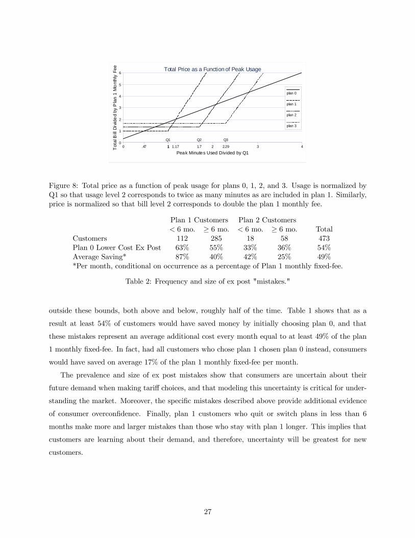
Total Price as a Function of Peak Usage

Figure 8: Total price as a function of peak usage for plans 0, 1, 2, and 3. Usage is normalized byQ1 so that usage level 2 corresponds to twice as many minutes as are included in plan 1. Similarly,price is normalized so that bill level 2 corresponds to double the plan 1 monthly fee.

Plan 1 Customers Plan 2 Customers< 6 mo. ≥ 6 mo. < 6 mo. ≥ 6 mo. Total

Customers 112 285 18 58 473Plan 0 Lower Cost Ex Post 63% 55% 33% 36% 54%Average Saving* 87% 40% 42% 25% 49%*Per month, conditional on occurrence as a percentage of Plan 1 monthly fixed-fee.

Table 2: Frequency and size of ex post "mistakes."

outside these bounds, both above and below, roughly half of the time. Table 1 shows that as a

result at least 54% of customers would have saved money by initially choosing plan 0, and that

these mistakes represent an average additional cost every month equal to at least 49% of the plan

1 monthly fixed-fee. In fact, had all customers who chose plan 1 chosen plan 0 instead, consumers

would have saved on average 17% of the plan 1 monthly fixed-fee per month.

The prevalence and size of ex post mistakes show that consumers are uncertain about their

future demand when making tariff choices, and that modeling this uncertainty is critical for under-

standing the market. Moreover, the specific mistakes described above provide additional evidence

of consumer overconfidence. Finally, plan 1 customers who quit or switch plans in less than 6

months make more and larger mistakes than those who stay with plan 1 longer. This implies that

customers are learning about their demand, and therefore, uncertainty will be greatest for new

customers.

27

8 Extensions

8.1 Multi-Tariff Menu

The primary model presented in this paper assumes that consumers have homogeneous priors ex

ante, and therefore firms offer only a single tariff. In reality consumers have heterogenous priors,

and as a result, are offered menus of multiple tariffs.

So rather than assuming that at time one all consumers have homogenous prior F (θ), assume

that each consumer receives a private signal s ∼ G (s) prior to choosing a tariff. The signal s does

not enter payoffs directly, but is informative about θ ∼ F (θ|s). The simplest ordering to consideris that in which signals are ordered by FOSD26 so that F (θ|s) ≤ F (θ|s) for all s ≥ s. Consumers

are overconfident in the sense that consumers’ conditional priors F ∗ (θ|s) cross the true conditionalpriors F (θ|s) once from below at θ∗ (s) in such a manner that preserves the FOSD ordering.

Extending the model in this direction now requires separate treatment for the monopoly and

perfect competition market conditions. For the case of perfect competition, by specifying marginal

costs which are not too small,27 examples can easily be constructed in which consumers who receive

signal s are offered the tariff described by the primary model in this paper as if they were the only

type.

The equilibrium tariff menu for one such example is illustrated by Figure 9. This is a variation

of the example presented in Section 4.5: As in column 2 of Figure 5, marginal cost c is $0.035, and

consumers are highly overconfident (∆ = 0.25). However, here consumers receive one of three signals

ex ante, low, medium, or high, which correspond to future θ being distributed uniformly over the

interval£−12 ,

12

¤, [0, 1], or

£12 ,32

¤respectively. This example yields a tariff menu qualitatively similar

to cellular phone service tariff menus. Moreover, the predicted usage distributions of customers on

each tariff are ordered by strict first order stochastic dominance.

For marginal costs close to zero, a menu of tariffs that are each individually optimal for a

homogeneous ex ante population would not be incentive compatible.28 In this case, solving for the

equilibrium tariff menu is left for future research.

For the case of monopoly, the single tariff model considered in this paper can be extended to

multiple tariffs following the approach of Courty and Li (2000). The details of this extension are

contained in a secondary appendix available from the author upon request. In this case it can be

26This assumption is weaker than affiliation between θ and s.

27 In most examples, the downward first-period incentive compatibility constraints will be satisfied, and the upwardincentive compatibility constraints will be as well if costs are increasing sufficiently fast.

28The upward first-period incentive-compatibility constraints would fail.

28

400 600 800 1000 1200quantity

20

40

60

80

100

$

FC = $25; c = $0.035; D= 0.25

Figure 9: Total pricing for a 3-tariff menu under perfect competition. Solid portionsof the tariffs are uniquely optimal. Dashed portions of the tariffs are illustrativeextensions where no consumption takes place. The straight line shows total costs.

shown that virtual surplus is given by equation (10).

Ψ (s, q, θ) = V (q, θ)− C (q)− Vθ (q, θ)

(1−G (s)

g (s)

∂∂s [1− F ∗ (θ|s)]

f (θ|s) +F ∗ (θ|s)− F (θ|s)

f (θ|s)

)(10)

The bracketed term now includes the information rent term 1−G(s)g(s)

∂∂s[1−F∗(θ|s)]f(θ|s) which arises

in Courty and Li’s (2000) model, and the perception gap term F∗(θ|s)−F (θ|s)f(θ|s) which arises in the

single tariff model with overconfidence. The optimal tariff maximizes virtual surplus subject to

the constraints of free disposal, as well as first and second period global incentive compatibility.

The constraint that allocation q (s, θ) be non-decreasing in θ remains necessary and sufficient for

second period incentive compatibility, and thus may be imposed through ironing if it is violated.

As in Courty and Li’s (2000) model, allocation q (s, θ) non-decreasing in signal s is sufficient but

not necessary for first period global incentive compatibility.

Now, however, general examples for which Courty and Li (2000) were able to show the relaxed

solution was non-decreasing in signal s may violate this sufficient condition given high enough levels

of overconfidence. This is because for high levels of overconfidence, the relaxed solution involves

marginal prices near the monopoly price for each particular minute as discussed in Section 5. Since

monopoly price increases with demand, this implies types with higher signals should face higher

marginal prices at a given quantity, and therefore consume less for a given θ. This is unfortunate,

29

because in these cases it is not known what the optimal tariff will look like.29

For specific cases in which the allocation of the relaxed solution is non-decreasing in signal s,

marginal price is given by equation (11) if it is well defined, where θ = θ (s, q).

Pq(s, q) =Max

⎧⎨⎩0, Vq (q, θ)−Cq (q)− Vqθ (q, θ)

⎧⎨⎩1−G(s)g(s)

∂∂s[1−F∗(θ|s)]f(θ|s)

+F∗(θ|s)−F (θ|s)f(θ|s)

⎫⎬⎭⎫⎬⎭ (11)

This shows that even for marginal cost equal to zero, types with signals below the maximum s will

face tariffs that have initially positive marginal prices, prior to entering a range of zero marginal

price. Otherwise each tariff on the menu will be qualitatively similar to that described by the single

tariff model.

8.2 Heterogeneous Overconfidence

Consider the case where fraction α of consumers share the firm’s prior F (θ), while fraction (1− α)

are overconfident and have an alternate prior F ∗ (θ). Under perfect competition, firms offer correct-

prior types and overconfident types separate tariffs identical to those offered when consumers are

homogeneous. Types with correct priors are offered price equal to cost©qFB (θ) , C

¡qFB (θ)

¢ª,

just as if all consumers had correct beliefs. Overconfident types are offered the equilibrium tariff©q∗ (θ) , PC (θ)

ªcharacterized in Section 4, just as if all consumers were overconfident.

Note that the firm earns the same profit on a given tariff from a participating consumer with

correct prior and a participating overconfident consumer. This is because both have the same true

type distribution F (θ) from the firm’s perspective, and therefore the same allocation q (θ) and

payment P (θ) distributions. Thus the constraint set of zero-profit tariffs is the same regardless of

whether a firm is serving consumers with correct priors or overconfident consumers.

Because the allocations qFB and q∗ each maximize the perceived expected utilities of their

intended consumers over the same constraint set, consumers cannot believe themselves to be strictly

better off under the other types’ tariff. Consumers with correct priors prefer the standard tariff since

E£SFB

¤≥ E [S∗], and overconfident types prefer the overconfident tariff since E [Ψ∗] ≥ E

£ΨFB

¤.

Under monopoly, there is one simple benchmark case where incentive compatibility of the

homogenous tariffs is similarly guaranteed. Whenever overconfident types correctly estimate the

surplus generated by the first best allocation:30 E∗£SFB

¤= E

£SFB

¤, in equilibrium correct-prior

29Global incentive compatibility would need to be checked directly, and if it failed an ironing procedure could notbe used to find the optimal tariff because monotonicity is not necessary.

30When marginal costs are zero, the benchmark E∗£SFB

¤= E

£SFB

¤implies consumers correctly estimate their

expected value of consuming up to their satiation points.

30

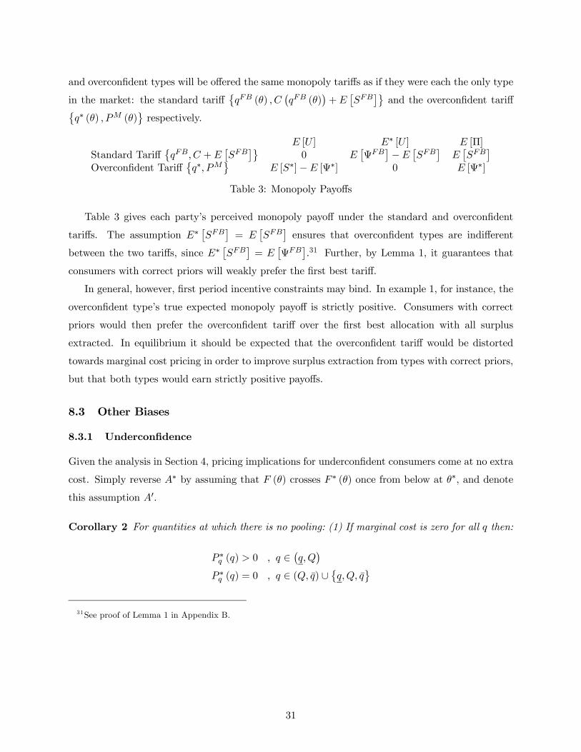
and overconfident types will be offered the same monopoly tariffs as if they were each the only type

in the market: the standard tariff©qFB (θ) , C

¡qFB (θ)

¢+E

£SFB

¤ªand the overconfident tariff©

q∗ (θ) , PM (θ)ªrespectively.

E [U ] E∗ [U ] E [Π]Standard Tariff

©qFB, C +E

£SFB

¤ª0 E

£ΨFB

¤−E

£SFB

¤E£SFB

¤Overconfident Tariff

©q∗, PM

ªE [S∗]−E [Ψ∗] 0 E [Ψ∗]

Table 3: Monopoly Payoffs

Table 3 gives each party’s perceived monopoly payoff under the standard and overconfident

tariffs. The assumption E∗£SFB

¤= E

£SFB

¤ensures that overconfident types are indifferent

between the two tariffs, since E∗£SFB

¤= E

£ΨFB

¤.31 Further, by Lemma 1, it guarantees that

consumers with correct priors will weakly prefer the first best tariff.

In general, however, first period incentive constraints may bind. In example 1, for instance, the

overconfident type’s true expected monopoly payoff is strictly positive. Consumers with correct

priors would then prefer the overconfident tariff over the first best allocation with all surplus

extracted. In equilibrium it should be expected that the overconfident tariff would be distorted

towards marginal cost pricing in order to improve surplus extraction from types with correct priors,

but that both types would earn strictly positive payoffs.

8.3 Other Biases

8.3.1 Underconfidence

Given the analysis in Section 4, pricing implications for underconfident consumers come at no extra

cost. Simply reverse A∗ by assuming that F (θ) crosses F ∗ (θ) once from below at θ∗, and denote

this assumption A0.

Corollary 2 For quantities at which there is no pooling: (1) If marginal cost is zero for all q then:

P ∗q (q) > 0 , q ∈¡q,Q

¢P ∗q (q) = 0 , q ∈ (Q, q) ∪

©q,Q, q

ª31See proof of Lemma 1 in Appendix B.

31

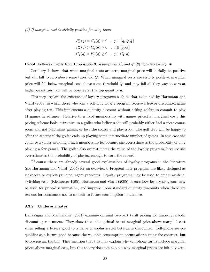
(2) If marginal cost is strictly positive for all q then:

P ∗q (q) = Cq (q) > 0 , q ∈©q,Q, q

ªP ∗q (q) > Cq (q) > 0 , q ∈

¡q,Q

¢Cq (q) > P ∗q (q) ≥ 0 , q ∈ (Q, q)

Proof. Follows directly from Proposition 3, assumption A0, and q∗ (θ) non-decreasing.

Corollary 2 shows that when marginal costs are zero, marginal price will initially be positive

but will fall to zero above some threshold Q. When marginal costs are strictly positive, marginal

price will fall below marginal cost above some threshold Q, and may fall all they way to zero at

higher quantities, but will be positive at the top quantity q.

This may explain the existence of loyalty programs such as that examined by Hartmann and

Viard (2005) in which those who join a golf-club loyalty program receive a free or discounted game

after playing ten. This implements a quantity discount without asking golfers to commit to play

11 games in advance. Relative to a fixed membership with games priced at marginal cost, this

pricing scheme looks attractive to a golfer who believes she will probably either find a nicer course

soon, and not play many games, or love the course and play a lot. The golf club will be happy to

offer the scheme if the golfer ends up playing some intermediate number of games. In this case the

golfer overvalues avoiding a high membership fee because she overestimates the probability of only

playing a few games. The golfer also overestimates the value of the loyalty program, because she

overestimates the probability of playing enough to earn the reward.

Of course there are already several good explanations of loyalty programs in the literature

(see Hartmann and Viard (2005) for an overview). Frequent flyer programs are likely designed as

kickbacks to exploit principal agent problems. Loyalty programs may be used to create artificial

switching costs (Klemperer 1995). Hartmann and Viard (2005) discuss how loyalty programs may

be used for price-discrimination, and improve upon standard quantity discounts when there are

reasons for consumers not to commit to future consumption in advance.

8.3.2 Underestimates

DellaVigna and Malmendier (2004) examine optimal two-part tariff pricing for quasi-hyperbolic

discounting consumers. They show that it is optimal to set marginal price above marginal cost

when selling a leisure good to a naive or sophisticated beta-delta discounter. Cell-phone service

qualifies as a leisure good because the valuable consumption occurs after signing the contract, but

before paying the bill. They mention that this may explain why cell phone tariffs include marginal

prices above marginal cost, but this theory does not explain why marginal prices are initially zero.

32

Aside from the different welfare implications, in the context of the model in this paper, naive

beta-delta discounters are essentially consumers who systematically underestimate their demand

at the time of contracting. That is, their prior F ∗ (θ) is first order stochastically dominated by

the firm’s belief F (θ). In this case F ∗ (θ) ≥ F (θ) for all θ, and therefore marginal price would be

predicted to be above marginal cost for all q.

The assumption in this paper that consumers are overconfident (A*) implies that consumers

underestimate demand conditional on it being high (θ > θ∗), but overestimate demand conditional

on it being low (θ < θ∗). The underestimation of demand above θ∗ drives marginal price above

marginal cost at high quantities, as would naive beta-delta discounting. It is the overestimation of

demand below θ∗ that drives the region of zero marginal price at low quantities. Thus the balanced

over and underestimation of demand captured by overconfidence is necessary for the result.

9 Conclusion

This paper has shown that given overconfident consumers, low marginal costs, and free disposal,

optimal pricing involves included minutes at zero marginal price. This provides a promising ex-

planation for the three-part tariff menus observed in the cellular phone services market. Empirical

evidence shows that consumer usage patterns are consistent with the explanation, and in particular,

that ex post "mistakes" by consumers are consistent with the underlying assumption of overcon-

fidence. Although an alternative common-prior explanation exists, it appears to be inconsistent

with consumer usage patterns. The model presented here is broadly applicable beyond cellular

services, and is potentially relevant in any market in which consumers commit to a contract while

they are uncertain about their eventual demand. In particular, the model can explain the use of

three-part tariffs for other communication services such as internet access, a range of rental services,

consumer credit card debt, and an increasing number of other services. Finally, if consumers are

underconfident rather than overconfident, the model can explain the implementation of quantity

discounts through loyalty programs.

33

10 Appendices

A Pooling

As it was omitted from the main text, a characterization of pooling quantities when the monotonic-

ity constraint binds is provided below in Proposition 4. This is useful because it facilitates the

calculation of pooling quantities in numerical examples.

Proposition 4 Assuming that there is no pooling at either endpoint©θ, θª, on any interior interval

[θ1, θ2] ⊆ int¡£θ, θ¤¢such that the monotonicity constraint is binding inside, but not just outside

the interval, the equilibrium allocation is constant at some level q∗ (θ) = q for all θ ∈ [θ1, θ2].Further, the pooling quantity q and bounds of the pooling interval [θ1, θ2] must satisfy equations

(12)-(13):32

qR (θ1) = qR (θ2) = q (12)Z θ2

θ1

Ψq (q, θ) f (θ) dθ = 0 (13)

Proof. Given the result in Proposition 2, the proof is omitted as it closely follows ironing results

for the standard screening model. See for example the analogous proof given in Fudenberg and

Tirole (1991), appendix to chapter 7.

Proposition 3 characterizes marginal pricing at quantities for which there is no pooling, and

states that marginal price will jump discretely upwards at quantities where there is pooling. It

is therefore interesting to know when qR (θ) will be increasing, and when qR (θ) will violate the

monotonicity constraint so that the equilibrium allocation q∗ (θ)must be ironed and involve pooling.

I hinted earlier that pooling is related to high levels of overconfidence. This section addresses the

issue rigorously. First, a preliminary result is required. Lemma 2 compares the relaxed allocation

to the first best allocation, showing that the relaxed allocation is above first best whenever F (θ) >

F ∗ (θ) and is below first best whenever F (θ) < F ∗ (θ):

Lemma 2 Given maintained assumptions:

qR (θ)

⎧⎪⎪⎨⎪⎪⎩≥¨ qFB (θ)

= qFB (θ)

< qFB (θ)

F (θ) > F ∗ (θ)

F (θ) = F ∗ (θ)

F (θ) < F ∗ (θ)

(¨) strict iff Cq

¡qFB (θ)

¢> 0

32Note that equation 13 requires that the first order condition which the relaxed solution satisfies when constraintsare not binding must be satisfied on average over pooling intervals.

34

Proof. See Appendix B.

Given that F ∗ (θ) crosses F (θ) once from below (A*), the relationship between the relaxed

allocation and first best given in Lemma 2 leads to the conclusion that qR (θ) is strictly increasing

near the bottom θ and near the top θ. While this does not entirely rule out pooling at the endpoints

in equilibrium, it does place restrictions on such pooling described in Proposition 5.

Proposition 5 (1) There exists some δ > 0 such that qR (θ) is strictly increasing both in a region

[θ, θ + δ) near θ, and in a region¡θ − δ, θ

¤near θ. (2) If there is pooling at the bottom over the

interval [θ, θ2], then the pooling region extends above θ∗ (θ2 > θ∗). Similarly, if there is pooling

at the top over the interval£θ1, θ

¤, then the pooling region extends below θ∗ (θ1 < θ∗). (3) There

cannot be pooling both at the bottom θ and at the top θ. Therefore there is efficiency at the top or

the bottom. (4) When marginal cost is zero for all q, (Cq (q) = 0 : ∀q), there is no pooling at thetop.

Proof. (1) Following Lemma 2, qR (θ) is equal to first best at θ and weakly above first best just

above θ. This implies that qR (θ) must be increasing weakly faster than qFB (θ) at θ. Similarly,

since qR (θ) is equal to first best at θ and strictly below first best just below θ (Lemma 2), qR (θ)

must be increasing strictly faster than first best at θ. Since qFB (θ) is strictly increasing for all

θ (Appendix B Lemma 3), this implies that the relaxed allocation qR (θ) is strictly increasing in

neighborhoods of θ and θ.

(2)-(4) See Appendix B.

While Proposition 5 does not entirely rule out pooling at the endpoints in equilibrium (in fact

it is likely to occur if θ∗ is very close to either endpoint), it suggests that it is not unreasonable to

focus on cases in which there is no pooling at the endpoints.

More can be said about pooling when consumers either have nearly correct beliefs, or are

extremely overconfident. When consumers’ prior is close to that of the firm, the relaxed solution

is strictly increasing. When consumers are extremely overconfident such that their prior is close

to the belief that θ = θ∗ with probability one, the relaxed solution is strictly decreasing at θ∗. In

this case the equilibrium allocation q∗ (θ) involves pooling at θ∗. These results and the notion of

"closeness" are made precise in Proposition 6.

The intuition for the first result is simply that when the consumers’ prior is close to that of the

firm, the relaxed solution will be close to first best, which is strictly increasing. The intuition for

the second result follows from Lemma 2, which shows that qR (θ) ≥ qFB (θ) when F (θ) ≥ F ∗ (θ)

and qR (θ) < qFB (θ) when F (θ) < F ∗ (θ). In the limit, when the consumers’ prior is the belief

that θ = θ∗ with probability one, [F (θ)− F ∗ (θ)] discontinuously falls below zero at θ∗. Thus the

35

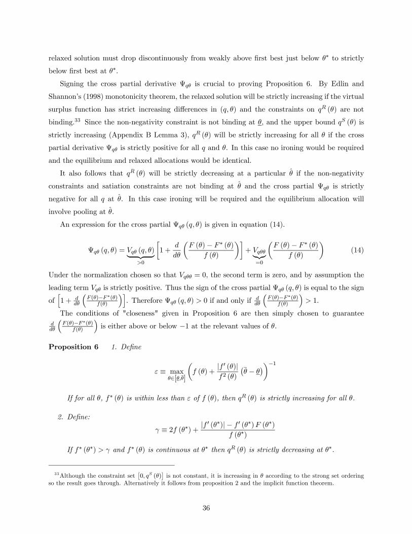
relaxed solution must drop discontinuously from weakly above first best just below θ∗ to strictly

below first best at θ∗.

Signing the cross partial derivative Ψqθ is crucial to proving Proposition 6. By Edlin and

Shannon’s (1998) monotonicity theorem, the relaxed solution will be strictly increasing if the virtual

surplus function has strict increasing differences in (q, θ) and the constraints on qR (θ) are not

binding.33 Since the non-negativity constraint is not binding at θ, and the upper bound qS (θ) is

strictly increasing (Appendix B Lemma 3), qR (θ) will be strictly increasing for all θ if the cross

partial derivative Ψqθ is strictly positive for all q and θ. In this case no ironing would be required

and the equilibrium and relaxed allocations would be identical.

It also follows that qR (θ) will be strictly decreasing at a particular θ if the non-negativity

constraints and satiation constraints are not binding at θ and the cross partial Ψqθ is strictly

negative for all q at θ. In this case ironing will be required and the equilibrium allocation will

involve pooling at θ.

An expression for the cross partial Ψqθ (q, θ) is given in equation (14).

Ψqθ (q, θ) = Vqθ (q, θ)| {z }>0

∙1 +

d

dθ

µF (θ)− F ∗ (θ)

f (θ)

¶¸+ Vqθθ|{z}

=0

µF (θ)− F ∗ (θ)

f (θ)

¶(14)

Under the normalization chosen so that Vqθθ = 0, the second term is zero, and by assumption the

leading term Vqθ is strictly positive. Thus the sign of the cross partial Ψqθ (q, θ) is equal to the sign

ofh1 + d

dθ

³F (θ)−F ∗(θ)

f(θ)

´i. Therefore Ψqθ (q, θ) > 0 if and only if d

dθ

³F (θ)−F ∗(θ)

f(θ)

´> 1.

The conditions of "closeness" given in Proposition 6 are then simply chosen to guaranteeddθ

³F (θ)−F ∗(θ)

f(θ)

´is either above or below −1 at the relevant values of θ.

Proposition 6 1. Define

ε ≡ maxθ∈[θ,θ]

µf (θ) +

|f 0 (θ)|f2 (θ)

¡θ − θ

¢¶−1

If for all θ, f∗ (θ) is within less than ε of f (θ), then qR (θ) is strictly increasing for all θ.

2. Define:

γ ≡ 2f (θ∗) + |f0 (θ∗)|− f 0 (θ∗)F (θ∗)

f (θ∗)

If f∗ (θ∗) > γ and f∗ (θ) is continuous at θ∗ then qR (θ) is strictly decreasing at θ∗.

33Although the constraint set£0, qS (θ)

¤is not constant, it is increasing in θ according to the strong set ordering

so the result goes through. Alternatively it follows from proposition 2 and the implicit function theorem.

36

Proof. See Appendix B.

The conditions for "closeness" given in Proposition 6 may look somewhat daunting. For the

special case where F (θ) is uniform on [0, 1], however, they simplify dramatically. In this case qR (θ)

is non-decreasing if f∗ (θ) ∈ [0, 2] for all θ. Further qR (θ) is strictly decreasing at θ∗ if f∗ (θ∗) > 2.Figure 10 illustrates many of the results discussed in this section. The figure covers the same

example developed in Section 4.5, in this case with higher marginal costs of c = $0.15. Low

overconfidence ∆ = 0.75 is depicted in the left hand column and high overconfidence ∆ = 0.25

is depicted in the right hand column. The figure plots the allocation in the top row and the

distribution of consumers over quantity in the bottom row. Lemma 2 which compared the relaxed

allocation to first best is born out in plots A and B.

Moreover the prediction of Proposition 6 that pooling occur at θ∗ for high overconfidence, and

nowhere for low overconfidence is also born out. In the left hand column under low overconfidence,

plot A shows the allocation is strictly increasing for all types, and Plot C shows the cumulative

density of quantity is increasing continuously. In the right hand column under high overconfidence,

however, Plot B shows that the allocation is constant at some level Q over a region including θ∗.

Further, the plot D shows that the cumulative density of quantity increases discretely at Q due

to the atom of consumers pooling at this quantity. This corresponds to the discrete increase in

marginal price in plot D of Figure 5.

In this simple example, pooling occurs at θ∗ if and only if ∆ ≤ 12 , and the satiation constraint

binds somewhere if and only if c ≤ min©38 ,34 (1−∆)

ª. Figure 11 illustrates these regions of pooling

and satiation on the parameter space.

B Proofs

B.1 Proof of Proposition 1

Proof.

1. Expected firm profits are always equal to the difference between expected surplus and the con-

sumers’ true expected utility: E [Π (θ)] = E [S (θ)]−E [U (θ)]. Participation constraints underboth monopoly and perfect competition will bind. Thus under monopoly, since E∗ [U (θ)] = 0,

the firm’s expected profit can be rewritten as: E [Π (θ)] = E [S (θ)] + E∗ [U (θ)] − E [U (θ)].

Similarly under perfection competition, since E [Π (θ)] = 0, the consumers’ perceived expected

utility may be rewritten as: E∗ [U (θ)] = E [S (θ)] +E∗ [U (θ)]−E [U (θ)].

Local incentive compatibility requires that U 0 (θ) = Vθ (q (θ) , θ). Thus by applying the FTC,

taking expectations, and integrating by parts, consumer’s true expected utility from the

37

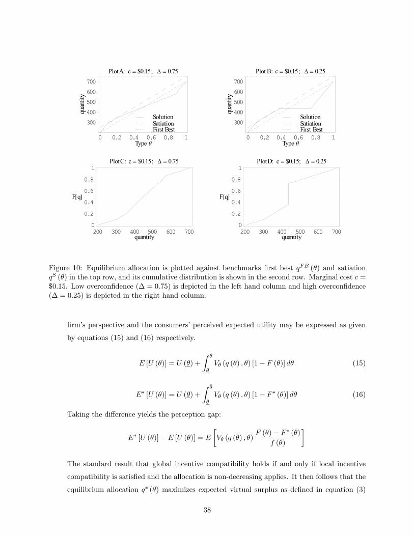
200 300 400 500 600 700quantity

0

0.2

0.4

0.6

0.8

1

F@qD

PlotC: c = $0.15; D = 0.75

200 300 400 500 600 700quantity

0

0.2

0.4

0.6

0.8

1

F@qD

PlotD: c = $0.15; D = 0.25

0 0.2 0.4 0.6 0.8 1Type q

300

400

500

600

700ytitnauq

PlotA: c = $0.15; D = 0.75

First BestSatiationSolution

0 0.2 0.4 0.6 0.8 1Type q

300

400

500

600

700

ytitnauq

Plot B: c = $0.15; D = 0.25

First BestSatiationSolution

Figure 10: Equilibrium allocation is plotted against benchmarks first best qFB (θ) and satiationqS (θ) in the top row, and its cumulative distribution is shown in the second row. Marginal cost c =$0.15. Low overconfidence (∆ = 0.75) is depicted in the left hand column and high overconfidence(∆ = 0.25) is depicted in the right hand column.

firm’s perspective and the consumers’ perceived expected utility may be expressed as given

by equations (15) and (16) respectively.

E [U (θ)] = U (θ) +

Z θ

θVθ (q (θ) , θ) [1− F (θ)] dθ (15)

E∗ [U (θ)] = U (θ) +

Z θ

θVθ (q (θ) , θ) [1− F ∗ (θ)] dθ (16)

Taking the difference yields the perception gap:

E∗ [U (θ)]−E [U (θ)] = E

∙Vθ (q (θ) , θ)

F (θ)− F ∗ (θ)

f (θ)

¸

The standard result that global incentive compatibility holds if and only if local incentive

compatibility is satisfied and the allocation is non-decreasing applies. It then follows that the

equilibrium allocation q∗ (θ) maximizes expected virtual surplus as defined in equation (3)

38

½ 10Δ

c

0½ 10Δ

c

½ 10Δ

c

0

Satiation but no Pooling

Pooling butno Satiation

No Pooling or Satiation

Pooling &Satiation

Example

No Overconfidence

ExtremeOverconfidence

38

Figure 11: This figure maps out regions in the parameter space of the running example in whichpooling occurs and in which the satiation constraint is binding for some types.

subject to the remaining constraints of monotonicity, non-negativity, and free disposal.

2. The equilibrium allocation q∗ (θ) implicitly defines equilibrium payments P ∗ (θ) through the

local incentive compatibility and the binding participation constraints. In particular, applying

local incentive compatibility and the FTC, the payment function can be backed out up to a

fixed fee U (θ):

P ∗ (θ) = V (q∗ (θ) , θ)−Z θ

θVθ (q

∗ (z) , z) dz − U (θ) (17)

Further, equation (16) can be rearranged to solve for the utility of the lowest type in terms

E∗ [U (θ)]:

U (θ) = E∗ [U (θ)]−E

∙Vθ (q (θ) , θ)

1− F ∗ (θ)

f (θ)

¸(18)

Under monopoly, the consumers’ binding participation constraint is E∗ [U (θ)] = 0. Combing

this fact with equations (17) and (18) yields the monopoly payment:

PM (θ) = V (q∗ (θ) , θ)−Z θ

θVθ (q

∗ (z) , z) dz +E

∙Vθ (q (θ) , θ)

1− F ∗ (θ)

f (θ)

¸

Under perfect competition, firm profits are zero rather than E [Ψ (q∗ (θ) , θ)], so the payment

must be lower by the fixed amount E [Ψ (q∗ (θ) , θ)]:

PC (θ) = PM (θ)−E [Ψ (q∗ (θ) , θ)]

39

3. Differentiating equation (17) for P ∗ (θ) and making a change of variables yields the desired

result:d

dqP ∗ (q) = Vq (q, θ (q))

This is valid for quantities at which there is no pooling, where θ (q) is a well defined function.

B.2 Small Lemma 3

The satiation quantity qS (θ) must be characterized prior to solving for the equilibrium allocation

q∗ (θ) as it is the upper bound of the constraint set. Moreover, both satiation qS (θ) and first best

qFB (θ) quantities are important benchmarks to which q∗ (θ) is compared in the paper. Lemma 3

therefore gives relevant properties of each.

Lemma 3 1. Satiation qS (θ) and first best qFB (θ) quantities are continuously differentiable,

strictly positive, and strictly increasing.

2. Satiation quantity is higher than first best quantity, and strictly so when marginal costs are

strictly positive at qFB.

qS (θ)

⎧⎨⎩ = qFB (θ) Cq

¡qFB (θ)

¢= 0

> qFB (θ) Cq

¡qFB (θ)

¢> 0

Proof. Given maintained assumptions, qS (θ) and qFB (θ) exist, and are continuous functions.

Moreover they are everywhere characterized by the first order conditions Vq¡qS (θ) , θ

¢= 0 and

Sq¡qFB (θ) , θ

¢= 0 respectively. The implicit function theorem implies qS (θ) and qFB (θ) are both

continuously differentiable with derivatives:

d

dθqS = −Vqθ

Vqq

d

dθqFB = − Vqθ

Vqq −Cqq

It then follows that both are strictly increasing. Further, when Cq

¡qFB (θ)

¢= 0, the first order

condition Sq¡qFB (θ) , θ

¢= 0 implies that Vq

¡qFB (θ) , θ

¢= 0. This is simply the first order

condition for qS (θ) which must be satisfied, so qS (θ) = qFB (θ). When Cq

¡qFB (θ)

¢> 0, the first

order condition Sq¡qFB (θ) , θ

¢= 0 implies that Vq

¡qFB (θ) , θ

¢> 0. Since V is concave in q, this

implies that qS (θ) > qFB (θ).

40

B.3 Proof of Proposition 2

Proof. Under maintained assumptions, the constraint setD (θ) =£0, qS (θ)

¤is convex and compact

valued, continuous, and non-empty. Further, virtual surplus Ψ (q, θ) is continuous and strictly

concave in q:

Ψqq (q, θ) = Vqq (q, θ)| {z }<0

− Cqq (q)| {z }≥0

+ Vqqθ (q, θ)| {z }=0

F (θ)− F ∗ (θ)

f (θ)< 0

Therefore qR is a continuous function. (Note that this is where the stricter assumption Vqqθ = 0 is

needed rather than the standard assumption Vqqθ ≤ 0.)Since Ψ (q, θ) is twice continuously differentiable and strictly concave in q for all θ, qR (θ) is

characterized by the first order condition Ψq (q, θ) = 0 unless either the non-negativity or free

disposal constraints are binding.

Over the interior of any interval for which qR is characterized the FOC Ψq

¡qR, θ

¢= 0 and F ∗ is

continuously differentiable, then by the implicit function theorem qR is continuously differentiable

with derivative ddθq

R = −Ψqθ

Ψqq. Since qS (θ) is continuously differentiable (Lemma 3) this implies

that qR (θ) is piecewise smooth. Kinks may occur when qR hits the constraints 0 or qS , or a kink

in F ∗ when the constraints are not binding.

B.4 Proof of Proposition 3

Proof. (1) Following Proposition 1, at non-pooling quantities marginal price is equal to Vq (q, θ (q)).

Thus at pooling quantity q, marginal price must increase discontinuously since above and below q

marginal price is given by Vq (q, inf {θ (q)}) and Vq (q, sup {θ (q)}) respectively and by assumptionVqθ > 0.

(2) Further, at non-pooling quantities the non-negativity and monotonicity constraints are not

binding and q∗ (θ) = qR (θ) by Proposition 2 part 2. Thus by Proposition 2 part 1, either (i) the

equilibrium allocation is characterized by the first order condition Ψq (q, θ) = 0, or (ii) the satiation

constraint is binding and marginal price is zero since the satiation quantity is characterized by

Vq¡qS (θ) , θ

¢= 0. In the former case, the first order condition can be solved for Vq (q, θ), and

therefore marginal price:

Vq (q, θ) = Cq (q) + Vqθ (q, θ)F ∗ (θ)− F (θ)

f (θ)

WhenhCq (q) + Vqθ (q, θ (q))

F∗(θ(q))−F (θ(q))f(θ(q))

iis negative, the first order condition Ψq = 0 im-

plies Vq (q, θ) is negative and therefore q ≥ qS (θ). This is precisely when the satiation con-

straint binds, ensuring marginal price to be weakly positive. Thus marginal price is equal to

41

hCq (q) + Vqθ (q, θ (q))

F∗(θ(q))−F (θ(q))f(θ(q))

iwhenever that quantity is positive, and zero otherwise.

(3) Since θ (q) is a continuous function at non-pooling quantities, marginal price is as well. Thus

payment P ∗ (θ (q)) is continuously differentiable at non-pooling quantities. Moreover, incentive

compatibility requires that types who pool at the same quantity pay the same price. Thus P ∗ (θ (q))

is well defined and continuous at pooling quantities.

B.5 Proof of Lemma 1

Proof. Given the characterization of q∗ in Proposition 1, expected virtual surplus must be weakly

higher under the equilibrium allocation than under the first best allocation: E [Ψ∗] ≥ E£ΨFB

¤.

Moreover, under marginal cost pricing expected profits are equal to the fixed fee regardless of

the prior over θ. Thus under the first best allocation, the expected virtual surplus is equal to the

perceived expected surplus: E£ΨFB

¤= E∗

£UFB

¤+E

£ΠFB

¤= E∗

£UFB

¤+E∗

£ΠFB

¤= E∗

£SFB

¤.

Together this implies that E [Ψ∗] ≥ E∗£SFB

¤. The assumption E∗

£SFB

¤≥ E

£SFB

¤therefore

implies that the firm is better off: E [Ψ∗] ≥ E£SFB

¤. This in turn implies that consumers are

worse off since total welfare is lower.

B.6 Proof of Lemma 2

Proof. Part (1): The relaxed allocation maximizes virtual surplus Ψ (q, θ) within the constraint

set£0, qS (θ)

¤. By definition the first best allocation maximizes true surplus S (q, θ), but is not

constrained to be below qS (θ). However by Lemma 3, qFB (θ) ≤ qS (θ) so the first best allocation

must maximize surplus within the constraint set£0, qS (θ)

¤. Since the two allocations maximize

quantities which differ only by VθF (θ)−F ∗(θ)

f(θ) over the same constraint set the following trick can be

used.

Define φ (q, θ, β) such that φ (q, θ, 0) = S (q, θ) and φ (q, θ, 1) = Ψ (q, θ) as follows:

φ (q, θ, β) = V (q, θ)− C (q) + βVθF (θ)− F ∗ (θ)

f (θ)

The sign of the cross partial derivative φqβ then depends on the sign of [F (θ)− F ∗ (θ)]:

φqβ (q, θ, β) = Vqθ|{z}>0

F (θ)− F ∗ (θ)

f (θ)

As a result there are three cases to consider:

1. F (θ) = F ∗ (θ): In this case virtual surplus and true surplus are equal so qR (θ) = qFB (θ).

42

2. F (θ) > F ∗ (θ): In this case φ (q, θ, β) has strict increasing differences in (q, β). Topkis’s

(1978) monotone comparative statics result then implies that qR (θ) ≥ qFB (θ). When

Cq

¡qFB (θ)

¢= 0, Lemma 3 shows that qS (θ) = qFB (θ) and therefore the satiation con-

straint binds: qR (θ) = qFB (θ) = qS (θ). When Cq

¡qFB (θ)

¢> 0, Lemma 3 shows that

qS (θ) > qFB (θ). Therefore the satiation constraint is not binding at qFB (θ). Then since

φ (q, θ, β) is continuously differentiable in (q, β), Edlin and Shannon’s (1998) monotonicity

theorem guarantees the comparison is strict: qR (θ) > qFB (θ).

3. F (θ) < F ∗ (θ): In this case φ (q, θ, β) has strict decreasing differences in (q, β). Topkis’s

(1978) monotone comparative statics result then implies that qR (θ) ≤ qFB (θ). The compar-

ison is strict by Edlin and Shannon (1998) since φ (q, θ, β) is continuously differentiable in

(q, β), and the non-negativity constraint is not binding at qFB (θ) (Lemma 3).

B.7 Proof of Proposition 5

Proof. Part (1) See text.

Part (2) Assume the monotonicity constraint is binding at the bottom over the interval [θ, θ2],

but not just above θ2. It must be that q∗ (θ) ≤ qR (θ) since otherwise q∗ (θ) could be set equal to

qR (θ) without violating monotonicity. Then Propositions 2 and 4 require that:

qR (θ2) = q∗ (θ) ≤ qR (θ)

Together, Lemma 2 and Lemma 3 imply the following inequality holds for all θ ∈ (θ,θ∗]:

qR (θ) ≥ qFB (θ) > qFB (θ) = qR (θ)

Therefore, it must be that either θ2 =θ (there is not pooling) or θ2 > θ∗. The proof for the result

about pooling at the top is analogous.

Part (3): The proof of part (2) implies that if there were pooling at both the top and the

bottom, q∗ (θ) would have to be constant over the entire interval£θ, θ¤, and satisfy qR

¡θ¢≤

q∗ (θ) ≤ qR (θ). Together Lemma 2 and Lemma 3 imply that:

qR¡θ¢= qFB

¡θ¢> qFB (θ) = qR (θ)

so this is impossible.

43

Part (4) Following the proof of part (2), pooling at the top requires qR (θ1) ≥ qR¡θ¢for some

θ1 < θ∗. However, under zero marginal costs, Lemma 2 requires qR (θ) = qFB (θ) for all θ ∈ [θ, θ∗]as well as for θ = θ. Since qFB (θ) is strictly increasing by Lemma 3 no such θ1 exists.

B.8 Proof of Proposition 6

Proof. Define

ϕ (θ) ≡ F (θ)− F ∗ (θ)

f (θ)

then

ϕ0 (θ) =

µ1− f∗ (θ)

f (θ)

¶− f 0 (θ)

f2 (θ)[F (θ)− F ∗ (θ)]

Part (1): Following previous discussion, it is sufficient to show that ϕ0 (θ) > −1 or equivalently−ϕ0 (θ) < 1 for all θ.

−ϕ0 (θ) = −f (θ) [f (θ)− f∗ (θ)] +f 0 (θ)

f2 (θ)[F (θ)− F ∗ (θ)]

Since f (θ) > 0:

−ϕ0 (θ) ≤ f (θ) |f (θ)− f∗ (θ)|+ |f0 (θ)|

f2 (θ)|F (θ)− F ∗ (θ)|

Since it is given that |f (θ)− f∗ (θ)| < ε and this implies that |F (θ)− F ∗ (θ)| < ε¡θ − θ

¢:

−ϕ0 (θ) < f (θ) ε− f 0 (θ)

f2 (θ)ε¡θ − θ

¢= ε

µf (θ)− f 0 (θ)

f2 (θ)

¡θ − θ

¢¶

For ε ≡34maxθ∈[θ,θ]³f (θ) + |f 0(θ)|

f2(θ)

¡θ − θ

¢´−1this implies−ϕ0 (θ) < 1 and therefore qR (θ) is strictly

increasing for all θ.

Part (2): The first step is to show that ϕ0 (θ∗) < −1.

ϕ0 (θ) =

µ1− f∗ (θ)

f (θ)

¶− f 0 (θ)

f2 (θ)F (θ) +

f 0 (θ)

f2 (θ)F ∗ (θ)

Since it is given that f∗ (θ∗) > γ, it follows thatµ1− f∗ (θ∗)

f (θ∗)

¶<

µ1− γ

f (θ∗)

¶

34Note that ε is well defined since£θ, θ¤is compact and F ∈ C2 implies

µf (θ) +

|f0(θ)|f2(θ)

¡θ − θ

¢¶−1is continuous.

44

Further, since F ∗ (θ) ∈ [0, 1], it follows that

f 0 (θ)

f2 (θ)F ∗ (θ) ≤ |f

0 (θ)|f2 (θ)

Together this implies:

ϕ0 (θ∗) <

µ1− γ

f (θ∗)

¶− f 0 (θ∗)

f2 (θ∗)F (θ∗) +

|f 0 (θ∗)|f2 (θ∗)

=

µ1− γ

f (θ∗)

¶+|f 0 (θ∗)|− f 0 (θ∗)F (θ∗)

f (θ∗)

Substituting in γ = f (θ∗)³2 + |f 0(θ∗)|−f 0(θ∗)F (θ∗)

f2(θ∗)

´yields ϕ0 (θ∗) < −1.

The second step relies on Lemma 2. By Lemma 2, for some δ1 > 0 neither satiation nor

non-negativity constraints are binding on qR (θ) in the interval (θ∗, θ∗ + δ1). First, satiation is

not binding just above θ∗ since qR is below first best here (Lemma 2), which is always below the

satiation bound (Lemma 3). Second, non-negativity is not binding just to the right of θ∗ because

qR (θ∗) = qFB (θ∗) > 0 (Lemma 2 and Lemma 3) and qR (θ) is continuous (Proposition 2). Since

neither constraint is binding, for θ ∈ (θ∗, θ∗ + δ1), then in the same interval the implicit function

theorem implies qR (θ) = −Ψqθ(qR(θ),θ)Ψqq(qR(θ),θ)

(Proposition 2).

So following earlier discussion, qR (θ) is strictly decreasing in this interval if ϕ0 (θ) < −1. Byassumption f∗ (θ) is continuous at θ∗ which implies ϕ0 (θ) is continuous at θ∗as well. Therefore

for some δ2 > 0, ϕ0 (θ) < −1 just above θ∗ in the interval θ ∈ (θ∗, θ∗ + δ2). Therefore qR (θ) is

strictly decreasing in the interval (θ∗, θ∗ +min {δ1, δ2}) just above θ∗. Since qR (θ) is piecewise

smooth (Proposition 2), qR (θ) is either strictly decreasing at θ∗ or has a kink at θ∗ and is strictly

decreasing just above θ∗. In either case, monotonicity is violated at θ∗ and the equilibrium allocation

will involve pooling at θ∗.

45

References

Arkes, Hal R., “Overconfidence in judgemental forecasting,” in J. S. Armstrong, ed., Principles of Fore-

casting, Boston: Kluwer Academic Publishers, 2001, pp. 495—515.

Baron, D. P. and D. Besanko, “Regulation and Information in a Continuing Relationship,” Information

Economics and Policy, 1984, 1 (3).

Barrett, G.F. and S.G. Donald, “Consistent tests for stochastic dominance,” Econometrica, 2003, 71

(1), 71—104.

Bolger, Fergus and Dilek Onkal-Atay, “The effects of feedback on judgmental interval predictions,”

International Journal of Forecasting, 2004, 20 (1), 29—39.

Courty, Pascal and Hao Li, “Sequential screening,” Review of Economic Studies, 2000, 67 (4), 697—717.

Davidson, R. and J.Y. Duclos, “Statistical inference for stochastic dominance and for the measurement

of poverty and inequality,” Econometrica, 2000, 68 (6), 1435—1464.

DellaVigna, Stefano and Ulrike Malmendier, “Contract design and self-control: Theory and evidence,”

Quarterly Journal of Economics, 2004, 119 (2), 353—402.

Edlin, A.S. and C. Shannon, “Strict monotonicity in comparative statics,” Journal of Economic Theory,

1998, 81 (1), 201—219.

Fudenberg, Drew and Jean Tirole, Game theory, Cambridge, Mass.: MIT Press, 1991.

Griffin, Dale and Amos Tversky, “The Weighing of Evidence and the Determinants of Confidence,”

Cognitive Psychology, 1992, 24, 411—435.

Hartmann, Wesley R. and Brian V. Viard, “Quantity-Based Price Discrimination Using Frequency

Reward Programs,” working paper, Stanford University Graduate School of Business 2005.

Juslin, P., A. Winman, and H. Olsson, “Naive empiricism and dogmatism in confidence research: A

critical examination of the hard-easy effect,” Psychological Review, 2000, 107 (2), 384—396.

Kaur, A., B.L.S.P. Rao, and H. Singh, “Testing for Second-Order Stochastic Dominance of two Distri-

butions,” Econometric Theory, 1994, 10 (5), 849—866.

Klemperer, P., “Competition When Consumers Have Switching Costs: An Overview with Applications

to Industrial Organization, Macroeconomics, and International Trade,” Review of Economic Studies,

1995, 62 (4), 515—539.

Koenig, David, “Blockbuster plans to end late fees in 2005,” December 14, 2004 2004.

Lambrecht, Anja, Katja Seim, and Bernd Skiera, “Does Uncertainty Matter? Consumer Behavior

under Three-Part Tariffs,” working paper 2005.

Leonard, Daniel and Ngo van Long, Optimal control theory and static optimization in economics,

Cambridge ; New York: Cambridge University Press, 1992.

46

Lichtenstein, Sarah, Baruch Fischhoff, and Lawrence D. Phillips, “Calibration of probabilities:

The state of the art to 1980,” in Daniel Kahneman, Paul Slovic, and Amos Tversky, eds., Judgment

under uncertainty : heuristics and biases, Cambridge ; New York: Cambridge University Press, 1982,

pp. 306—334.

Loewenstein, G., T. O’Donoghue, and M. Rabin, “Projection bias in predicting future utility,” Quar-

terly Journal of Economics, 2003, 118 (4), 1209—1248.

Miravete, Eugenio J., “Choosing the wrong calling plan? Ignorance and learning,” American Economic

Review, 2003, 93 (1), 297—310.

Mirrlees, J. A., “An Exploration in Theory of Optimum Income Taxation,” Review of Economic Studies,

1971, 38 (114), 175—208.

Mussa, Michael and Sherwin Rosen, “Monopoly and Product Quality,” Journal of Economic Theory,

1978, 18 (2), 301—317.

Rochet, Jean-Charles and Lars Stole, “The Economics of Multidimensional Screening,” in M. Dewa-

tripont, Lars Peter Hansen, and Stephen J. Turnovsky, eds., Advances in economics and econometrics:

theory and applications - eighth world Congress, Vol. 36 of Econometric Society Monographs, New York:

Cambridge University Press, 2003.

Rothschild, Michael and Joseph E. Stiglitz, “Increasing Risk: I. A Definition,” Journal of Economic

Theory, 1970, 2 (3), 225—243.

Stole, Lars A., “Nonlinear Pricing and Oligopoly,” Journal of Economics and Management Strategy, 1995,

4 (4), 529—62.

Stoline, M.R. and H.K. Ury, “Tables of the Studentized Maximum Modulus Distribution and an Appli-

cation to Multiple Comparisons Among Means,” Technometrics, 1979, 21 (1), 87—93.

Topkis, Donald M., “Minimizing a Submodular Function on a Lattice,” Operations Research, 1978, 26,

305—321.

Tse, Y.K. and X.B. Zhang, “A Monte Carlo investigation of some tests for stochastic dominance,”

Journal of Statistical Computation and Simulation, 2004, 74 (5), 361—378.

47