scoping the impact tidal and wave energy · pdf fileon suspended sediment concentrations and...

143

SCOPING THE IMPACT TIDAL AND WAVE ENERGY EXTRACTION ON SUSPENDED SEDIMENT CONCENTRATIONS AND UNDERWATER LIGHT CLIMATE07M.R. Heath1, A.D. Sabatino1, N. Serpetti2, and R.B. O’Hara Murray3

1 DEPARTMENT OF MATHEMATICS AND STATISTICS, UNIVERSITY OF STRATHCLYDE, 16 RICHMOND STREET, GLASGOW, G1 1XQ

2 SCOTTISH ASSOCIATION FOR MARINE SCIENCE, SCOTTISH MARINE INSTITUTE, OBAN, PA37 1QA

3 MARINE SCOTLAND SCIENCE, SCOTTISH GOVERNMENT, MARINE LABORATORY, 375 VICTORIA ROAD, ABERDEEN, AB11 9DB

back to contents

144 07/ Scoping the impact tidal and wave energy extraction on suspended sediment concentrations and underwater light climate

07/1 INTRODUCTION

The depth to which sunlight penetrates below the sea surface is one of the key factors determining the species composition and productivity of marine ecosystems. The effects range from the rate and fate of primary production, through the performance of visual predators such as fish, the potential for refuge from predators by migrating to depth, to the scope for seabed stabilisation by algal mats. Light penetration depends partly on spectral absorption by seawater and dissolved substances, but mainly on the scattering caused by suspended particulate material (SPM). Some of this SPM may be of biological origin, but in coastal waters the majority is mineral material originating ultimately from seabed disturbance and land erosion, the latter being deposited in the sea by rivers and aerial processes. SPM is maintained in the water column or deposited on the seabed depending on combinations of hydrodynamic processes including baroclinic (density-driven) or barotropic (mainly tidal and wind driven) currents, and wave action (Ward et al. 1984; Huettel et al. 1996). Since tidal and wave energy extraction must alter these hydrodynamic properties at some scales depending on the nature of the extraction process, we can expect some kind of impact on the concentration of the SPM. If these are large enough, we may have to consider the extent to which these may impact the underwater light environment and the local or regional ecology.

Whilst several coupled hydrodynamic-sediment models exist to predict SPM distributions in aquatic systems, their skill level in open coastal and offshore marine waters is acknowledged to be relatively low. This is largely because the processes are not well understood and the formulations are largely based on empirical relationships rather than fundamental physical principles. The models are also highly demanding in terms of calibration data and computational resources. Hence their utility for predicting relatively subtle effects arising from changes in flow or wave environments due to energy extraction devices seems rather low. Here, we summarise the key mathematical functions describing the processes involved in sediment suspension, and propose a lightweight one-dimensional (vertical) model which can be used to scope the effects of changes in flow and wave energy on SPM.

07/2 BRIEF REVIEW OF PROCESSES AND EQUATIONS INVOLVED IN MODELLING SUSPENDED SEDIMENT PROCESSES

07/2.1 INITIATION OF PARTICLE MOVEMENT ON THE SEABED AND THE ERODIBILITY OF SEDIMENTS

With constant uniform water flow over a smooth bed, particle movement will occur when the instantaneous fluid force on a particle is larger than the instantaneous resisting force. The latter is related to the submerged particle size or weight and the friction coefficient. Cohesive forces are also important when the bed consists of appreciable amounts of clay and silt particles or biological material. The shear stress to which a particle is subjected is a function of its size, the flow speed, and the densities of the fluid and particles. The critical value of shear stress required to initiate motion is often estimated from the empirically-based ‘Shield diagram’ (Shields 1936), which relates a dimensionless measure of critical shear stress to the Reynolds number of a particle in a given flow.

The dimensionless Reynolds number is given by (Reynolds 1883):

where = the bed shear velocity (m.s-1), = fluid density (kg.m-3), = particle diameter (m), and

= kinematic viscosity (m2.s-1) of the fluid. The Reynolds number accounts for the ratio between the momentum forces with the viscous forces.

The bed shear velocity is related to the bed shear stress by:

The dimensionless Shield number or Shield stress is then given by

where is the density of sediment grains (kg.m-3), and is the acceleration due to gravity (m.s-2).

back to contents

14507/ Scoping the impact tidal and wave energy extraction on suspended sediment concentrations and underwater light climate

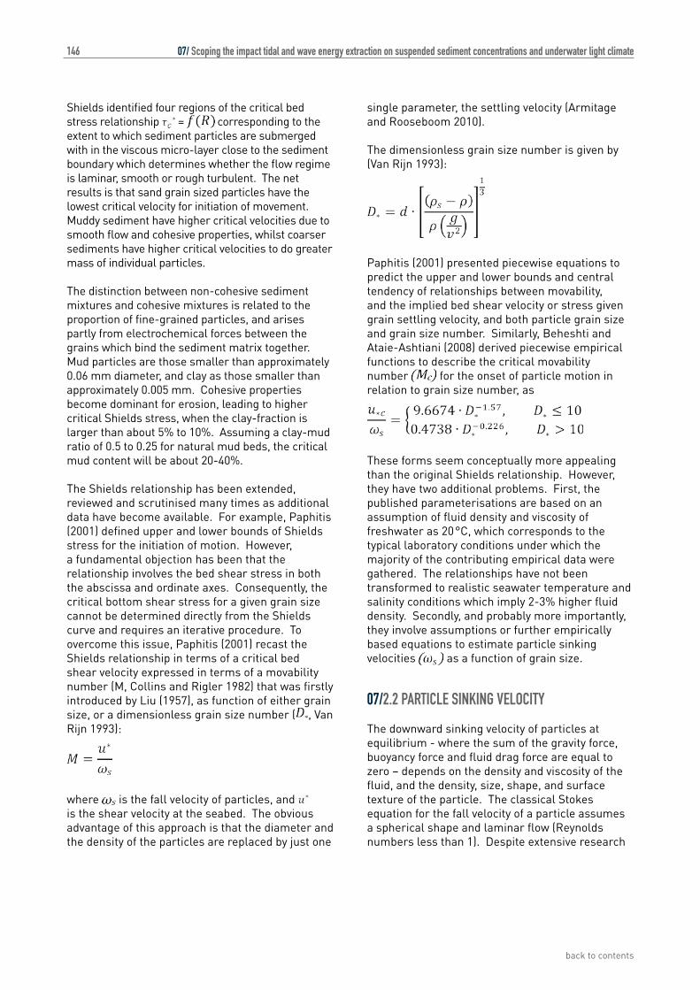
The critical value of Shield stress for the initiation of particle motion is typically estimated from an empirical relationship between and . An approximate parameterisation of this relationship is given by Wilcock et al (2009):

Movement of particles is assumed to be initiated when the shear stress is higher than the above threshold .

Fig 7.1 Shields diagram. Solid line represents the critical Shields stress for particle motion . Symbols represent three different particle grain diameters and two values of bed shear velocity: red = mud (40 μm), green = sand (300 μm), blue = pebble (1 cm); circles = bed shear velocity 10 cm.s-1; triangles = bed shear velocity 1 cm.s-1.

back to contents

146

Shields identified four regions of the critical bed stress relationship = corresponding to the extent to which sediment particles are submerged with in the viscous micro-layer close to the sediment boundary which determines whether the flow regime is laminar, smooth or rough turbulent. The net results is that sand grain sized particles have the lowest critical velocity for initiation of movement. Muddy sediment have higher critical velocities due to smooth flow and cohesive properties, whilst coarser sediments have higher critical velocities to do greater mass of individual particles.

The distinction between non-cohesive sediment mixtures and cohesive mixtures is related to the proportion of fine-grained particles, and arises partly from electrochemical forces between the grains which bind the sediment matrix together. Mud particles are those smaller than approximately 0.06 mm diameter, and clay as those smaller than approximately 0.005 mm. Cohesive properties become dominant for erosion, leading to higher critical Shields stress, when the clay-fraction is larger than about 5% to 10%. Assuming a clay-mud ratio of 0.5 to 0.25 for natural mud beds, the critical mud content will be about 20-40%.

The Shields relationship has been extended, reviewed and scrutinised many times as additional data have become available. For example, Paphitis (2001) defined upper and lower bounds of Shields stress for the initiation of motion. However, a fundamental objection has been that the relationship involves the bed shear stress in both the abscissa and ordinate axes. Consequently, the critical bottom shear stress for a given grain size cannot be determined directly from the Shields curve and requires an iterative procedure. To overcome this issue, Paphitis (2001) recast the Shields relationship in terms of a critical bed shear velocity expressed in terms of a movability number (M, Collins and Rigler 1982) that was firstly introduced by Liu (1957), as function of either grain size, or a dimensionless grain size number ( , Van Rijn 1993):

where is the fall velocity of particles, and is the shear velocity at the seabed. The obvious advantage of this approach is that the diameter and the density of the particles are replaced by just one

single parameter, the settling velocity (Armitage and Rooseboom 2010).

The dimensionless grain size number is given by (Van Rijn 1993):

Paphitis (2001) presented piecewise equations to predict the upper and lower bounds and central tendency of relationships between movability, and the implied bed shear velocity or stress given grain settling velocity, and both particle grain size and grain size number. Similarly, Beheshti and Ataie-Ashtiani (2008) derived piecewise empirical functions to describe the critical movability number for the onset of particle motion in relation to grain size number, as

These forms seem conceptually more appealing than the original Shields relationship. However, they have two additional problems. First, the published parameterisations are based on an assumption of fluid density and viscosity of freshwater as 20°C, which corresponds to the typical laboratory conditions under which the majority of the contributing empirical data were gathered. The relationships have not been transformed to realistic seawater temperature and salinity conditions which imply 2-3% higher fluid density. Secondly, and probably more importantly, they involve assumptions or further empirically based equations to estimate particle sinking velocities as a function of grain size.

07/2.2 PARTICLE SINKING VELOCITY

The downward sinking velocity of particles at equilibrium - where the sum of the gravity force, buoyancy force and fluid drag force are equal to zero – depends on the density and viscosity of the fluid, and the density, size, shape, and surface texture of the particle. The classical Stokes equation for the fall velocity of a particle assumes a spherical shape and laminar flow (Reynolds numbers less than 1). Despite extensive research


back to contents

147

there is still no analytical solution to predict the fall velocity of natural shaped particle, or particles large enough to generate turbulent flow. Many investigators have proposed empirically based relationships to predict particle fall velocities with varying degrees of complication and success. Sadat-Helbar et al. (2009) reviewed 17 published relationships and identified that developed by Wu and Wang (2006) as being one of the most reliable formulations for the sinking velocity:

where , and are coefficients and represents the nominal grain size diameter. Empirical calibration against a wide range of sediments provided coefficient values as:

where is the Corey shape factor – typically taken to be 0.7 (Camenen 2007).

Sadat-Helbar et al. (2009) also provided their own somewhat simpler generalised piecewise relationship in where fall velocity increases as a power function of particle diameter, without incorporating any shape parameter terms:

where

and

Although these relationships perform reasonably well at predicting the central tendency of the accumulated experiment data on settling velocities of naturally occurring mineral grains, there remains a considerable amount

of unexplained variability. Since the settling velocity appears as the denominator in the grain mobility function and, for mud grains, is a small number relative to the bed shear velocity, even small variations can have a large effect on predictions of the critical shear stress required to initiate motion of given grain sizes. Hence, despite the objections and the many proposed alternatives, the original Shields relationship describing the critical stress for initiation of particle motion remains in widespread use.

07/2.3 ERODIBILITY OF MIXED GRAIN SIZE SEDIMENT

The Shields and other equivalent relationships refer to unimodal sediment grain sizes, whilst natural marine sediments are frequently composed of multiple modes spanning a wide range of sizes, and often layers of different composition. Laboratory and field observations have shown that erosion of sand beds is inhibited by the presence of the mud particles, and vice versa, so that the shear stress required to initiate particle motion is significantly increased (Van Rijn 1993, Bartzke et al. 2013, Mitchener and Torfs 1996). In addition, material in different layers may exhibit widely varying erosion shear thresholds, especially when recently deposited fine grained material is overlaid onto older coarse beds (Amos et al 1992, El Ganaoui et al. 2004).

07/2.4 EFFECTS OF BED-FORMS

The morphology of the sea bed (plane or rippled bed) has a significant role in the erodibility of sediments. The architecture of the sea bed controls the near-bed velocity profile, the shear stresses and the turbulence and, thereby, the mixing and transport of the sediment particles. Ripples in the sediment surface reduce the near-bed velocities, but it enhances the bed-shear stresses, turbulence and the entrainment of sediment particles, resulting in larger overall suspension rates. Several types of bed forms can be identified, depending on the type of wave-current motion and the bed material composition. For fine sand (grain size 0.1 to 0.3 mm), as bed shear increases beyond the critical Shields stress the surface initially develops rolling grain ripples, then vortex ripples, and finally plane bed with sheet flow of sediment


back to contents

148

grains. Soulsby and Whitehouse (2005) developed algorithms for predicting bedforms in sandy sediments in relation to bed shear velocities, and their evolution during time-varying flows.

07/2.5 EFFECTS OF CONSOLIDATION ON SEDIMENT ERODIBILITY

The empirically-based Shields relationship takes account of cohesive forces between particle grains, but not the effects of consolidation. Various processes lead to natural sediments becoming more resistant to erosion post-deposition, producing marked deviations from the expected Shields particle motion thresholds. Compaction occurs when sediment volume is reduced and density increased due to expulsion of pore water by stress from overlying material. Other natural processes which lead to the consolidation of sediments and their increased resistance to erosion include chemical dissolution and/or precipitation of minerals, and biological activity. These processes are referred to as diagenesis in geological and ecological literature.

No general relationships to represent consolidation and its effect on sediment erodibility have emerged (McCave 1984). The early formulation of Partheniades (1965) remains widely used in models of sediment erosion (e.g. Whitehouse et al. 2000; Ribbe and Holloway 2001; Kuhrts et al., 2004; Pandoe and Edge 2004; Van den Eynde 2004), though it merely deals the problem by posing an unknown site and time specific parameter (E) to represent erodibility:

where is the erosion rate (kg.m-2.s-1), is the erodibility (kg.m-2.s-1), and is the critical threshold for erosion, equivalent to the Shields critical stress.

For a soft or partly consolidate sediment:

(Parchure and Mehta 1985)

Biological processes leading to consolidation may take many forms and are therefore extremely

difficult to generalise. Secretion of sticky organic molecules by microbes (Grant and Gust 1987, Lubarsky et al. 2010), benthic algae and microbes clogging the pore spaces and binding grains together (Austen et al 1999, Paterson and Black 1999, Nowell et al. 1981, Sutherland et al. 1998), and forming mats on the sediment surface all lead to inhibition of sediment erosion (Oppenheim and Paterson 1990, Fonseca 1989, Paterson 1989). Living algal mats are most prevalent in shallow waters since the micro-organisms concerned require light to photosynthesise. Other biological processes may have the opposite effect on sediment erodibility due to de-stabilisation of the sediment structure. These include bioturbation by burrowing and sediment ingesting macrofauna and meiofauna which reprocesses sediment into faecal granules (Lumborg et al. 2006, Montague 1986, Rowden et al. 1998).

The key issues is the extent of spatial and temporal variability in biologically induced consolidation and erodibility. The problem is well known and extensively studies in tidal mud-flats and shallow estuaries where the sediments are predominantly fine cohesive muds and the effects of biological activity are very obvious (Andersen 2001, Widdows et al. 2000, Le Hir & Karlinkow 1992, Austen et al. 1999, Paterson et al. 2000). In fact, it has become apparent that seasonal variation in erodibility mediated by biological activity may be the dominant factor controlling water turbidity in shallow tidal regions such as the Wadden Sea (De Vires and Borsje 2008, Borsje et al. 2008, Lumborg et al. 2006). Various measurements have been investigated as potential indicators of biologically-mediated erodibility, for example, algal pigment content of sediments (Riethmuller et al. 2000), but so far none have shown general applicability.

Early models of sediment suspension and transport in deeper open shelf systems generally assumed that spatial, and especially temporal, variability in biological consolidation and erodibility of sediments could be regarded as negligible (e.g. Pohlmann and Puls 1994, Ribbe and Holloway 2001, Kuhrts et al. 2004, Pandoe & Edge 2004, van den Eynde 2004). However, recent research shows that this cannot be assumed (Stevens et al. 2007, Briggs et al. 2015). Operational formulations for including variability of biologically-mediated consolidation in shelf sea sediment models is lacking. For example, Dobrynin (2009) found that


back to contents

149

a model of suspended sediment concentrations in the southern North Sea was unable to explain the distribution of surface concentrations derived from satellite remote sensing without resorting to alternative summer and winter parameterisations of erodibility.

07/2.6 LIFTING OF BED-LOAD PARTICLES INTO THE WATER COLUMN

When the value of the bed-shear velocity becomes sufficiently high relative to the particle fall velocity, the bed-load particles can be lifted into suspension. Usually, the behaviour of the suspended sediment particles is described in terms of the sediment concentration, which is the solid volume (m³) per unit fluid volume (m³) or the solid mass (kg) per unit fluid volume (m³). Observations show that the suspended sediment concentrations decrease with altitude up from the bed . The rate of decrease depends on the fall velocity of particles

and the vertical distribution of vertical diffusivity (Ks) through the water column.

The vertical flux of particulate mass can be described by the differential equation:

or

Where is the concentration at altitude above the seabed, and is the concentration at a reference altitude .

Predictions of vertical distributions of concentration therefore depend on assumptions about the vertical profile of diffusivity. Commonly used alternatives are to assume a constant diffusivity with depth, a linear decrease or a parabolic variation with peak diffusivity in mid-water.

With a linear diffusivity assumption, the concentration profile is given by

Where is the shear velocity at the seabed, is the von Kármán constant (0.4), and is a

coefficient relating eddy viscosity to eddy diffusivity (taken to be 1) (Rouse 1937, Van Rijn 1984, 1993).

The exponent / ( · · ) is referred to as the Rouse number.

Alternative assumptions regarding the vertical distribution of diffusivity give different expectations for the vertical profile of concentration, but the Rouse approach is most commonly applied.

Sensitivity analysis of the Rouse profile combined with the dependency of fall velocity on particle size shows that suspended sediment concentration profiles are likely to be highly sensitive to the grain size composition of sediments. Particles larger than approximately 0.1 mm are likely to remain concentrated close to the seabed except at high bed shear velocities (>10 cm.s-1). On the other hand, particles smaller than 0.06 mm, which make up the majority of muddy sediments in shelf seas, are likely to be lifted throughout the water column by shear velocities between 0.25 and 2.5 cm.s-1. With respect to the underwater light climate, the fine particles (<0.1 mm) are of most interest. At equivalent weight or volumetric concentrations in the water column, fine particles create more light scattering than coarse particles.

07/2.7 PARTICLE AGGREGATION IN THE WATER COLUMN

Particle-particle collisions during suspension in the water column may lead to aggregation and formation of flocs with potentially enhanced sinking rates, depending on the physical cohesive properties of particle grains and their stickiness due to biological coatings (e.g. Krone 1978, Andersen and Pejrup 2002, Mehta 1989; Winterwerp 2002; You 2004). The probability of collisions will be a function of the suspended sediment concentration. Experimental studies have found that settling velocity of for mud and silt particles is independent of concentration below 0.4 g/l. Between 0.4 and 2.0 g/l, settling velocity increases with concentration due to flocculation. Above 2.0 g/l settling velocity rapidly decreases due to break-up of flocs, flocs mutual hindrance and interactions between the flows around adjacent ones that tend to increase upward friction (Cancino and Neves 1999).


back to contents

150

An empirical relationship describing this process (Burt 1986) is of the form:

where and are constants, and lies between a lower threshold for particle-particle interactions, and an upper threshold at which particles begin to interfere and the effective settling velocity is reduced. The upper concentration corresponds to values found in e.g. mud slides, where the water-sediment mixture forms a super-dense liquid (e.g. Richardson and Zaki 1954), and is not relevant in typical shelf-sea marine situations.

07/2.8 LATERAL TRANSPORT AND TIME-DEPENDENT VERTICAL PROFILES OF SUSPENDED SEDIMENT

The velocity of suspended particles in a longitudinal direction is almost equal to the fluid velocity. So lateral transport of suspended sediment is simply the product of the vertical profile of sediment concentration and the vertical profile of water velocity (Van Rijn 1993). Hence, horizontal bed-load transport is relatively easily modelled because vertical processes affecting the particles are limited to the onset and cessation of motion on the seabed. However, suspended loads require time to adjust to changing conditions as particles are redistributed vertically in response to fluctuating conditions. Effective modelling of suspended sediment transport therefore requires dynamic representation of vertical convection-diffusion processes in order to resolve short term fluctuations in vertical concentration gradients.

In accelerating flows there always is a net vertical upward transport of sediment particles due to turbulence-related diffusive processes, which continues as long as the sediment transport capacity exceeds the actual transport rate. Conversely, during decelerating flow, there is a net downward sediment transport because particle sinking dominates, yielding smaller concentrations and transport rates. As a result, empirical studies show that sediment concentrations over, for example, a fine sand bed show a continuous adjustment to oscillating flow velocities, such as tidal flows, with a lag period in the range of 0 to 60 minutes. The time lag period is equivalent to the interval between maximum flow and the point at

which the transport capacity is equal to the actual transport rate. In the case of case of fine grained sediments or deep water columns, the settling process can continue during the slack water period giving a large time lag, which is then defined as the period between the time of zero transport capacity and the start of a new erosion cycle. Time lag effects can be neglected for sediments larger than about 0.3 mm for which the settling velocity is large, so that bed-load transport of coarse-grain sediments can be effectively modelled using a quasi-steady state approach (Van Rijn 1984, 1993).

07/3 SCOPING THE IMPACT OF WAVE AND TIDAL ENERGY EXTRACTION ON SUSPENDED SEDIMENT CONCENTRATIONS.

07/3.1 SIMPLE 1-DIMENSIONAL SUSPENDED SEDIMENT MODEL

Formally, simulation of the impact of wave and/or tidal energy extraction on suspended sediment concentrations requires the solution of equations representing erosion and deposition of sediment from the seabed, together with partial differential equations at each node in a 3-dimensional water column grid, describing the vertical and horizontal fluxes of particles. The latter depends on advection, convection, diffusion and settling velocities (e.g. Teisson 1991). All of this adds considerably to the already intensive computational and parameterisation demands of solving the hydrodynamic equations for wave propagation, and wind-driven and tidal current velocities at sufficiently high resolution to be of value for studying the impact of energy extraction devices. There are several models available for this task (e.g. Gerritsen et al. 2000, Mercier and Delhez 2007), including the MIKE by DHI Mud Transport Module (Danish Hydraulics Institute 2013). However, the task of calibrating the parameters of such models requires considerable investment in field data collection and model run-time, and none yet include adequate or any representation of the seasonality of sediment erodibility due to biological processes which is emerging from recent field investigations as a key issue for sediment dynamics. Hence, we propose here a lightweight, one-dimensional (vertical), modelling approach for basic scoping of the impact of energy extraction, incorporating simple caricatures of the basic


back to contents

151

erosion and deposition processes outlined in the review above.

The approach is to predict an instantaneous vertical profile of suspended sediment, given seabed depth, shear and the mud content of seabed sediment, incorporating time-dependent erodibility and a time-series autocorrelation effect for the bed-stress to caricature the lag effects arising from the dynamics of erosion and deposition. Clearly, this approach cannot take account of lateral transport of suspended sediment, so its use must be limited to area where the majority of sediment material in the water column arises from seabed local resuspension rather than horizontal transport.

Input variables

Mean sea surface height above the seabed Seabed sediment mud content (proportion by

weight of grain size <0.06 mm) Bed shear stress at time t, where t is in days

from 1 January in some reference year)

Parameters given as physical constants

Density of sediment material (2650 kg.m-3) Density of seawater (1026 kg.m-3 at salinity 35

and 10 °C) von Kármán constant (0.4),

Parameters requiring to be fitted or assumed

Autocorrelation time scale for bed stress hindcasting

Decay rate for bed stress hindcasting Scaling coefficient

Particle sinking rate Seabed mud content exponent term Bed stress exponent term Sinking rate exponent term Time-varying erodibility exponent Phase shift for time-varying erodibility cycle

Intermediate terms

Exponentially declining time-weighting function Time weighted average bed stress Time weighted average bed shear velocity

Time-varying component of erodibility term Near-seabed (1 m altitude) suspended

sediment concentration

Output

Suspended sediment concentration at altitude above the seabed

Equations

To take account of the lag effect of fluctuating wave orbital velocities and tidal current speeds on the vertical profile of suspended sediment, we assume that the bed stress generating a vertical profile of suspended sediment is a time-weighted average of the stress over some period prior to the instant of prediction.

We define an exponentially declining time-weighting function

where t is a series of shear observation times prior to the instant at which a prediction is required, , and is a negative number representing the autocorrelation time scale relevant to the formation of the suspended sediment profile.

The time-weighted shear is then given by

The corresponding time weighted bed shear velocity is then given by:

Biological activity in the seabed sediment leading to natural consolidation and changes in erodibility is expected to follow a seasonal cycle dictated by temperature and the input of fresh organic matter settling from the spring and summer plankton blooms. We do not know the exact form of this, though observational data on phyto-detritus pigments in the sediments, oxygen consumption and nutrient fluxes indicate a peak of activity in June/July and a minimum in December/January. In addition, we know that pigment concentrations and microbial fluxes increased with the mud content of sediments


back to contents

152

(Serpetti et al. 2012, Serpetti 2012). So, we caricature the erodibility of sediments in two parts – a sediment dependent term (power function of mud content), and a time dependent term represented by a cosine function scaled to vary between 0.5 and 1.0, and phase shifted by a period

relative to the solar cycle:

Then, we represent the near-bed suspended sediment concentration by:

This expression contains three components: the scaling coefficient which equates the modelled concentration to observed measurement units; an erodibility term , and bed shear stress term which corresponds to the erosion rate expression of e.g. Partheniades (1965). We do not set an explicit threshold of shear stress for the initiation of particle motion, since we are not addressing sediment fluxes or steady state concentrations under constant flows. Rather, we aim to caricature transient concentrations in a time varying system, where the concentration near the seabed at any instant reflects the balance between deposition and erosion fluxes, and deposition fluxes include time-lagged signals of past erosion events.

The suspended sediment concentration at altitude , is then given by:

The exponent here corresponds to the Rouse number but including an expression to reflect increasing particle-particle aggregation in the water column with increasing sediment concentration (Burt 1986).

07/3.2 ESTIMATING BED SHEAR STRESS ( ) FROM TIME SERIES OF MODELLED OR OBSERVED TIDAL CURRENT AND WAVE PROPERTIES

In a natural situation the shear stress at the seabed is the result of velocities due to tidal currents, orbital velocities arising from wind and swell waves, and residual flows due to density gradients and surface wind forcing. Combining these components to predict the shear velocity in the boundary layer at the seabed, and hence the bed shear stress, is a challenging task. The methodology needs to take account of transitions between laminar, smooth and rough turbulent flows depending on flow velocity and bed roughness, as these have very different consequences for bed-shear. Most existing theories for wave-current interactions only deal with the rough-turbulent case. Computational oceanographic models for shelf seas typically use simple caricatures of the wave current interaction to estimate bed shear stress. For example, MIKE by DHI uses the radiative stress due to wave action to attenuate or amplify the bed stress due to tidal flow depending on the relative directions of the two.

07/3.2.1 CALCULATING BED SHEAR STRESS ARISING FROM TIDAL AND RESIDUAL CURRENTS

Seabed shear-stress ( , N.m-2) can be estimated from the vertically averaged current speed throughout the water column using the “law-of-the-wall” method (Soulsby and Clarke 2005) which assumes a logarithmic decrease in velocity with proximity to the sediment-water interface:

The calculation depends on whether the flow is taken to be laminar or turbulent. This is estimated from the Reynolds viscosity :

If is the vertically averaged current speed, h is the water column depth, is the kinematic viscosity (m2.s-1) of the fluid.Then,

If ̅ = 0, = 0


back to contents

153

If > 0, If ≤ 2000 then laminar flow and = If > 2000 then turbulent flow and (smooth bed surface)

(rough bed surface; = bed roughness length = d50/12)

where, is the fluid density (kg.m-3), and d50 is the median particle size on the seabed.

07/3.2.2 CALCULATING ORBITAL VELOCITIES BENEATH SURFACE SWELL AND WIND WAVES

Orbital velocities generated by surface waves penetrate into the water column, decreasing in amplitude with depth. Calculation of orbital velocities at the seabed given information on wave height, period and direction can be performed according to Soulsby (2006; summarising the work of Soulsby (1987) and Soulsby and Smallman (1986)). Combining orbital velocities with tidal current speeds to estimate bed shear stress can then be performed according to Soulsby and Clarke (2005; summarising earlier work by Soulsby (1995, 1997)).

Calculation of seabed orbital velocity (Uw) according to Soulsby (2006):

Peak wave period (s) Zero crossing period (s) Mean wave crossing period (s) Natural scaling period (s) Significant wave height (m)

= 9.81 Acceleration due to gravity (m.s-2) Wave orbital velocity (m.s-1)

For a JONSWAP spectrum it is a reasonable approximation to take

Different models and observational devices variously provide different indices of the wave spectrum. Hence, if only data on peak wave period

are available, then

If only data on mean wave period are available, then

Then:

And finally,

07/3.2.3 COMBINING BED STRESS ARISING FROM CURRENT FLOWS WITH STRESS DUE TO WAVE ORBITAL VELOCITIES For combining wave orbital velocity with tidal current velocity, to derive bed shear stress under laminar and turbulent flow regimes, refer to Appendix A (Algorithm for calculating mean, maximum and r.m.s bed shear-stresses for laminar, smooth-turbulent and rough-turbulent wave-plus-current flows) in Soulsby and Clarke (2006).


back to contents

154

07/4 EXAMPLE CASE STUDY OF PREDICTED SUSPENDED SEDIMENT CONCENTRATIONS COMPARED TO OBSERVED DATA

Vertical profiles of turbidity (Formazine Turbidity Units (FTU), proportional to SPM (g.m-3)) measured at 0.5 m depth intervals and up to weekly intervals over the period 2008-2011, at 9 coastal sites off Stonehaven (NE Scotland) by Marine Scotland Science, were available for parameterising the suspended sediment model. Full information on the sites, seabed sediment properties, and data collection methods are provided elsewhere (Bresnan et al. 2008, Serpetti et al. 2012, Serpetti 2012). The seabed sediment mud content of the sites ranged from 0.6 to 38%, and the water depth from 28-50 m. Methods are summarised in Appendix 1 but very briefly, time series of bed shear stress due to combined tidal currents and waves at each sampling site were simulated by a MIKE by DHI hydrodynamic

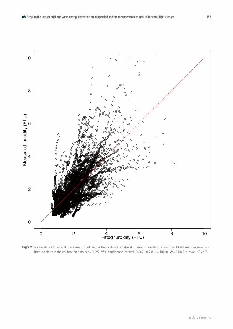
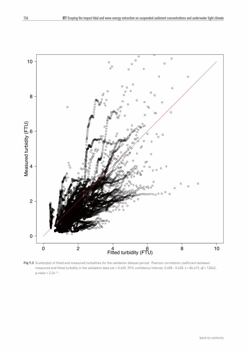
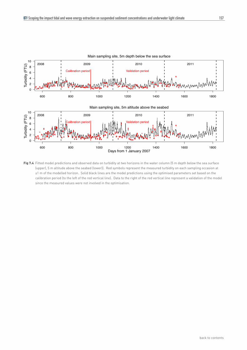
model (Sabatino et al. in preparation), and used as inputs to the sediment model. The model was then fitted to a calibration subset of the measured turbidity data by optimising the 9 parameters, and evaluated by comparing predicted turbidities with a validation subset of the measured data. The optimised parameter set provided a statistically highly significant fit of the model to both the calibration and the validation data subsets. The fitted parameters and standard errors are shown in Table 7.1 and full details are presented by Heath et al. (in preparation). Figure 7.2 shows the scatter plot of fitted and measured turbidities for the calibration period, and Figure 7.3 for the validation period. Figure 7.4 shows the fitted model for the calibration and validation periods as a time series at one of the sampling sites.

PARAMETER DESCRIPTION FITTED VALUE STANDARD ERROR Autocorrelation time scale for 4.723 0.207

bed stress hindcasting (d) Decay rate for bed stress hindcasting 0.652 2.281 Scaling coefficient 54.711 342.517

Particle sinking rate (m.s-1) 0.000210 Seabed mud content exponent term 0.1422 1.169 Bed stress exponent term 0.729 2.326 Sinking rate exponent term 0.823 0.295 Time-varying erodibility exponent 1.708 3.186 Phase shift for time-varying 0.0275 105.480

erodibility cycle (d)

Table 7.1 Parameter values and their standard deviations from Nelder Mead optimisation of the model to the calibration data set of measured turbidity profiles.


back to contents

155

0 2 4 6 8 10

0

2

4

6

8

10

Fitted turbidity (FTU)

Mea

sure

d tu

rbid

ity (F

TU)

Fig 7.2 Scatterplot of fitted and measured turbidities for the calibration dataset. Pearson correlation coefficient between measured and fitted turbidity in the calibration data set = 0.699, 95% confidence interval: 0.689 - 0.708. t = 104.04, df = 11343, p-value < 2.2e-16.


back to contents

156

0 2 4 6 8 10

0

2

4

6

8

10

Fitted turbidity (FTU)

Mea

sure

d tu

rbid

ity (F

TU)

Fig 7.3 Scatterplot of fitted and measured turbidities for the validation dataset period. Pearson correlation coefficient between measured and fitted turbidity in the validation data set = 0.620, 95% confidence interval: 0.608 - 0.630. t = 86.619, df = 12042, p-value < 2.2e-16.


back to contents

157

600 800 1000 1200 1400 1600 1800

0

2

4

6

8

10

Turb

idity

(FTU

)

Calibration period Validation period

2008 2009 2010 2011

Main sampling site, 5m depth below the sea surface

600 800 1000 1200 1400 1600 1800

0

2

4

6

8

10

Days from 1 January 2007

Turb

idity

(FTU

)

Calibration period Validation period

2008 2009 2010 2011

Main sampling site, 5m altitude above the seabed

Fig 7.4 Fitted model predictions and observed data on turbidity at two horizons in the water column (5 m depth below the sea surface (upper), 5 m altitude above the seabed (lower)). Red symbols represent the measured turbidity on each sampling occasion at ±1 m of the modelled horizon. Solid black lines are the model predictions using the optimised parameters set based on the calibration period (to the left of the red vertical line). Data to the right of the red vertical line represent a validation of the model since the measured values were not involved in the optimisation.


back to contents

158

07/4.1 TRANSLATING TURBIDITY INTO LIGHT PENETRATION DEPTH

Prior to the study period reported here (February 2007-May 2008), vertical profiles of photosynthetically active radiation (PAR) had been collected simultaneously at the seas surface and in vertical depth profiles on each weekly visit to one of the sampling sites. From these data, and empirical relationship between the vertical attenuation coefficient (natural logarithmic) of downwelling sea surface irradiation, and turbidity was established. The relationship also involved the in-situ concentration of phytoplankton chlorophyll which absorbs a portion of the downwelling light. The fitted relationship was:

PAR attenuation (m-1) = 0.1473 + 0.0620 · turbidity + 0.0082·chlorophyll; p < 0.001

where turbidity is given in FTU as elsewhere in this study, and chlorophyll in mg.m-3.

Using this relationship, we can estimate the depth of the 1% sea surface isolume in the absence of any chlorophyll from the turbidity at 5 m depth predicted by our sediment model (Figure 7.5). The 1% sea surface irradiance approximately corresponds to zero net photosynthesis i.e. gross photosynthetic uptake of carbon equals respiration. So the depth of this isolume is a measure of the euphotic zone thickness.

07/4.2 IMPACT OF TIDAL OR WAVE ENERGY EXTRACTION SCENARIOS

In order to scope the impact on euphotic zone thickness of the extraction of tidal or wave energy, we re-ran the bed shear stress calculation using the MIKE by DHI simulation outputs for the sampling sites, but assuming some removal of either tidal power by diminishing the depth mean current speed, or wave power by diminishing the significant wave height (but not the wave period).

Provide that the water depth is larger than half the wavelength, the power associated with a wave train is

Where is the power per metre of wave front (W.m-1), is the wave height and is the wave period.

The equivalent measure for a current flow (power per metre at the sea surface perpendicular to the flow) is given by:

where h is the seabed depth and V is the depth mean current speed.

Averaged over the three calendar years 2009, 2010 and 2011, the mean wave power at the sampling site illustrated in Figure 7.4 was 7.37 KW.m-1, s.d. 15.18 KW.m-1. The corresponding figure for the tidal flow was 20.49 KW.m-1, s.d. 11.65 KW.m-1.

Removing an arbitrary value of half of the total available wave power at this site (averaged over the three years = 3.685 KW.m-1) would be equivalent to reducing the significant wave height to

= 0.71 of the unexploited state. Removing the same quantity of power by attenuating the tidal flow would represent only an 18% draw-down of the long terms average current power, or a diminishing of the tidal speed to = 0.936 of the unexploited state.

We independently attenuated the significant wave height and the depth mean tidal current speed in the MIKE by DHI outputs, and recomputed the bed shear stress, the turbidity and the 1% irradiance depth for each case. The results showed that removing power equivalent to half of the wave power at this site had an imperceptible effect on the light environment (mean and s.d. of 1% irradiance depths: unexploited system 18.46 m s.d. 3.20 m; removing 50%l of wave power 18.98 m s.d. 3.20 m; removing equivalent power as tidal attenuation 18.87 m s.d. 3.08 m).

The wave power resource at the study site is small, so we also assessed the impact of removing a larger quantity of power (10 kW.m-1, approximately half of the long-term average tidal resource) purely by attenuating the tidal current speed


back to contents

159

600 800 1000 1200 1400 1600 1800

−30

−20

−10

0


Dep

th (m

) 2008 2009 2010 2011

Predicted depth of 1% sea surface isolume

600 800 1000 1200 1400 1600 1800

−30

−20

−10

0


Dep

th (m

) 2008 2009 2010 2011

Predicted depth of 1% sea surface isolume with energy extraction

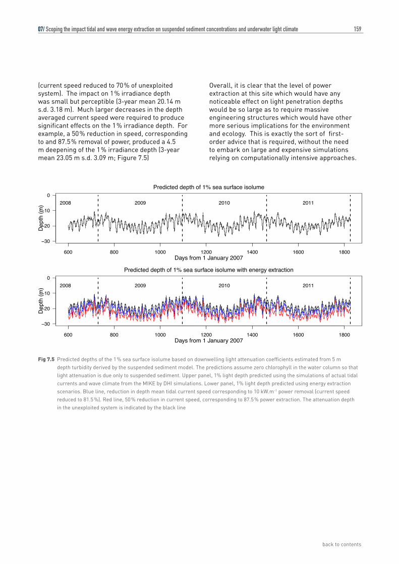
(current speed reduced to 70% of unexploited system). The impact on 1% irradiance depth was small but perceptible (3-year mean 20.14 m s.d. 3.18 m). Much larger decreases in the depth averaged current speed were required to produce significant effects on the 1% irradiance depth. For example, a 50% reduction in speed, corresponding to and 87.5% removal of power, produced a 4.5 m deepening of the 1% irradiance depth (3-year mean 23.05 m s.d. 3.09 m; Figure 7.5)

Overall, it is clear that the level of power extraction at this site which would have any noticeable effect on light penetration depths would be so large as to require massive engineering structures which would have other more serious implications for the environment and ecology. This is exactly the sort of first-order advice that is required, without the need to embark on large and expensive simulations relying on computationally intensive approaches.

Fig 7.5 Predicted depths of the 1% sea surface isolume based on downwelling light attenuation coefficients estimated from 5 m depth turbidity derived by the suspended sediment model. The predictions assume zero chlorophyll in the water column so that light attenuation is due only to suspended sediment. Upper panel, 1% light depth predicted using the simulations of actual tidal currents and wave climate from the MIKE by DHI simulations. Lower panel, 1% light depth predicted using energy extraction scenarios. Blue line, reduction in depth mean tidal current speed corresponding to 10 kW.m-1 power removal (current speed reduced to 81.5%). Red line, 50% reduction in current speed, corresponding to 87.5% power extraction. The attenuation depth in the unexploited system is indicated by the black line


back to contents

160

07/5 CONCLUSIONS

• The hydrodynamic principles of how particle grains are mobilised and lifted into suspension by current shear stresses, and settle back to the sea floor are well understood. Functional relationships can be effectively calibrated from controlled laboratory experiments.

• Real-world sediments composed of multiple grain-size classes in sorted layers, and containing active microbial ecosystems and macrofauna, cannot easily be replicated in laboratory experiments. There is a lack of understanding of how ecology affects sediment erodibility, but a growing realisation that it is important, even dominant in some situations, even in open shelf seas.

• Fully three-dimensional models of shelf sea suspended sediment are computationally intensive and require extensive data resources for calibration. Even so, none effectively include the seasonality of sediment erodibility due to biological consolidation processes.

• We propose a lightweight, one-dimensional (vertical) model of suspended sediment concentrations which caricatures the essential hydrodynamic processes, as a tool for quick assessments of the impact of energy extraction. In a case study, the model was parameterised by fitting to observational data, and showed that realistic levels of energy extraction are likely to produce only imperceptible effects on suspended sediment concentrations, light attenuation and predicted euphotic zone depths.

07/6 APPENDIX 1

Summary of methods for fitting and validating the sediment model at Stonehaven

Time series of depth averaged current speed and direction at 15 min intervals over 2008-2011 were reconstructed for each sampling site, using tidal harmonics extracted from a calibrated high resolution tidal model of the region constructed in MIKE 3D by DHI (Sabatino et al. submitted).

Significant wave height, mean wave period and mean wave direction at 15 min intervals from the UK Wavenet Firth of Forth monitoring buoy approximately 50km from the study area, were available for estimating wave orbital velocities at the sampling sites from July 2008 onwards. Time series of wave properties at each turbidity sampling site were predicted from the Wavenet buoy data using statistical relationships extracted from a spatially resolved, coupled wave-current model for the region constructed in MIKE by DHI (Sabatino et al., submitted).

Time series of orbital velocities at the seabed were derived from the estimated 15 minute significant wave height and peak wave period at each site using the algorithm of Soulsby (2006).

Time series of seabed shear stress at 15 min intervals were derived from the combination of depth averaged tidal current speed and direction and the wave orbital velocities and directions, following the algorithm detailed in Soulsby and Clarke 2005.


back to contents

161

The 371 vertical profiles of turbidity (30,433 individual measurements of turbidity at depth) were divided into two parts: data collected prior to 1 August 2009 (145 profiles, 12,044 measurements, referred to as the calibration period), and data collected after 1 August 2009 (226 profiles, 18,389 measurements, referred to as the validation period).

All 9 parameters of the model were fitted by minimising the r.m.s error between the entire calibration set of observed turbidity at depth at all sampling sites, and predicted values assuming the inputs of bed shear stress time series, seabed mud content, and sea surface altitude above the seabed at each site. Minimisation was performed by standard Nelder Mead optimisation using the ‘optim’ function in R,, with hessian matrix output so as to derive the standard errors of the parameters. The quality of the fit was measured with the Pearson correlation coefficient.

The fitted parameters of the model were then used to predict the time series of turbidity at two horizons in the water column at each site (5 m altitude above the seabed, and 5 m depth below the sea surface) for the full duration of the available bed shear stress time series at each site (July 2008 – December 2011). The predictions for the calibration and validation period at each site where then compared with the measured turbidity using the Pearson correlation coefficient.


back to contents

162

07/7 REFERENCES

Amos, C.L., Daborn, G.R., Christian, H.A., Atkinson, A. & Robertson, A. 1992. In situ erosion measurements on fine-grained sediments from the Bay of Fundy. Marine Geology 108, 175-196.

Andersen, T.J. 2001. Seasonal variation in erodibility of two temperate, microtidal mudflats. Estuarine, Coastal and Shelf Science 53, 1-12.

Andersen, T.J. & Pejrup, M., 2002. Biological mediation of the settling velocity of bed material eroded from an intertidal mudflat, the Danish Wadden Sea. Estuarine, Coastal and Shelf Science 54, 737-745.

Armitage, N. & Rooseboom, A., 2010. The link between Movability Number and Incipient Motion in river sediments. Water SA, 36(1), 89-96.

Austen, I., Andersen, T.J. & Edelvang, K. 1999. The influence of benthis diatoms and invertebrates on the erodibility of intertidal mudflats, the Danish Wadden Sea. Estuarine, Coastal and Shelf Science 49, 99-111.

Bartzke, G., Bryan, K.R., Pilditch, C.A. & Huhn, K. 2013. On the stabilizing influence of silt on sand beds. Journal of Sedimentary Research 83, 691-703.

Beheshti, A.A. & Ataie-Ashtiani, B. 2008. Analysis of threshold and incipient conditions for sediment movement. Coastal Engineering 55 (2008) 423–430.

Borsje, B.W., Hulscher, S.J.M.H., de Vries, M.B. & de Boer, G.J. 2008. Modelling large scale cohesive sediment transport by including biological acgtivity. River, Coastal and Estuarine Morphodynamics: RCEM 2007 – Dohmen-Janssen & Hulscher (eds). Taylor & Francos Group, London.p 255-262.

Bresnan, E., Hay, S., Hughes, S.L., Fraser, S., Rasmussen, J., Webster, L., Slesser, G., Dunn, J. & Heath, M.R. 2008. Seasonal and interannual variation in the phytoplankton community in the north east of Scotland. Journal of Sea Research 61, 17-25.

Briggs, K.B., Cartwright, G., Friedrichs, C.T. & Shivarudruppa, S. 2015. Biogenic effects on cohesive sediment erodibility resulting from recurring seasonal hypoxia on the Louisiana shelf. Continental Shelf Research 93, 17-26.

Burt, N. 1986. Field settling velocities of estuary muds. In: Estuarine cohesive sediment dynamnics, Ed. Mehta, A.J. Springer-Verlag, Berlin, Heidelberg, New York, Tokyo, p 126-150.

Camenen, B., 2007. Simple and general formula for the settling velocity of particles. J. Hydraul. Eng. 133 (2), 229–233.

Cancino, L. & Neves, R., 1999. Hydrodynamic and sediment suspension modelling in estuarine systems. Part I: description of the numerical models. Journal of Marine Systems 22, 105-116.

Collins, M.B. & Rigler, J.K., 1982. The use of settling velocity in defining the initiation of motion of heavy mineral grains, under unidirectional flow. Sedimentology 29, 419–426.

Danish Hydraulics Institute 2013. MIKE21 and MIKE3 Flow Model FM. Mud Transport Module Short Description. DHI Denmark, 12pp.

De Vires, M.B. & Borsje. B.W. 2008. Organisms influence fine sediment dynamics on basin scale. PECS 2008 – LIVERPOOL – UK.


back to contents

163

Dobrynin, M. 2009. Investigating the Dynamics of Suspended Particulate Matter in the North Sea Using a Hydrodynamic Transport Model and Satellite Data Assimilation. Dissertation zur Erlangung des Doktorgrades der Naturwissenschaften im Department Geowissenschaften der Universität Hamburg Petersburg. Hamburg 2009. 109pp.

El Ganaoui, O., Schaaff, E., Boyer, P., Amielh, M., Anselmet, F. & Grenz, C. 2004. The deposition and erosion of cohesive sediments determined by a multi-class model. Estuarine, Coastal and Shelf Science 60, 457-475.

Fonseca, M.S., 1989. Sediment stabilization by Halophila decipiens in comparison to other seagrasses. Estuarine Coastal Shelf Sci., 29: 501-507.

Gerritsen, H., Vos, R.J., van der Kaaij, T., Lane, A. & Boon, J.G. 2000. Suspended sediment modelling in a shelf sea North Sea. Coastal Engineering 41, 317–352.

Grant J. & Gust, G. 1987. Prediction of coastal sediment stability from photopigment purple sulphur bacteria. Nature 330, 244-246.

Heath, M.R., Sabatino, A.D., McCaig, C. & O’Hara Murray, R.B. (in preparation). Modelling spatial and temporal patterns of turbidity off the east coast of Scotland.

Huettel, M., Ziebis, W. & Forster, S., 1996. Flow-induced uptake of particulate matter in permeable sediments. Limnology and Oceanography, 41(2), 309-322.

Krone, R.B., 1978. Aggregation of suspended particles in estuaries. In: Kjerfve, B. (Ed.), Estuarine Transport Processes. University of South Carolina Press, Colombia, pp. 177-190.

Kuhrts, C., Fennel, W. & Seifert, T., 2004. Model studies of transport of sedimentary material in the western Baltic. Journal of Marine Systems 52, 167-190.

Le Hir, P. & Karlikow, N., 1992. Sediment transport modelling in a macrotidal estuary: do we need to account for consolidation processes? Proceedings of the Coastal Engineering Conference 3, 3121-3133.

Liu, H. K., 1957. Mechanics of sediment-ripple formation. Journal of the Hydraulics Division, 83(2), 1-23.

Lubarsky HV, Hubas C, Chocholek M, Larson F, Manz W, et al. (2010). The Stabilisation Potential of Individual and Mixed Assemblages of Natural Bacteria and Microalgae. PLoS ONE 5(11): e13794. doi:10.1371/journal.pone.0013794.

Lumborg, U., Andersen, T.J. & Pjirup, M. 2006. The effect of Hydrobia ulvae and microphytobenthos on cohesive sediment dynamics on an intertidal mudflat described by means of numerical modelling. Estuarine, Coastal and Shelf Science 68, 208-220.

McCave, N. 1984. Erosion, transport and deposition of fine-grained marine sediments. Geological Society, London, Special Publications 1984, v. 15, p. 35-69.

Mehta, A.J., 1989. On estuarine cohesive sediment suspension behaviour. Journal of Geographical Research 94 (C10), 14303e14314.

Mercier, C. & Delhez, E.J.M. 2007. Diagnosis of the sediment transport in the Belgian Coastal Zone. Estuarine, Coastal and Shelf Science 74, 670-683.


back to contents

164

Mitchener, H. & Torfs, H. 1996. Erosion of mud/sand mixtures. Coastal Eng., 29, 1–25.

Montague, C.L., 1986. Influence of biota on erodibility of sediments. In: Mehta, A.J. (Ed.), Estuarine Cohesive Sediment Dynamics. Springer-Verlag, Berlin, Heidelberg, NewYork, Tokyo, pp. 251-269.

Nowell, A.R.M., Jumars, P.A. & Eckman, J.E., 1981. Effects of biological activity on the entrainment of marine sediments. Marine Geology 42, 133-153.

Oppenheim, D.R. & Paterson, D.M., 1990. The fine structure of an algal mat from a freshwater maritime antarctic lake. Can. J. Bot., 68: 174-183.

Pandoe, W.W. & Edge, B.L., 2004. Cohesive sediment transport in the 3D hydrodynamic-baroclinic circulation model: study case for idealized tidal inlet. Ocean Engineering 31, 2227-2252.

Paphitis, D., 2001. Sediment movement under unidirectional flows: an assessment of empirical threshold curves Coas. Eng. 43, 227–245.

Parchure, T.M.. & Mehta, A.J. 1985. Erosion of soft cohesive sediment deposits. Journal of Hydraulic Engineering – ASCE 111 910), 1308-1326.

Partheniades, E. 1965. Erosion and Deposition of Cohesive Soils. Journal of the Hydraulics Division 91, 105-139.

Paterson, D. M. & Black, K.S. 1999. Water flow, sediment dynamics and benthic biology. Advances in Ecological Research 29. Academic Press. ISBN 0120139294.

Paterson, D. M., Tolhurst, T. J., Kelly, J.A., Honeywill, C., De Deckere, E.M.G.T., Huet, V., Shayler, S.A., Black, K.S., De Brouwer , J. & Davidson, I. 2000. Variations in sediment properties, Skeffling mudflat, Humber Estuary, UK. Continental Shelf Research 20, 1373-1396.

Paterson, D.M., 1989. Short-term changes in the erodibility of intertidal cohesive sediments related to the migratory behaviour of epipelic diatoms. Limnology and Oceanography 34, 223-234.

Pohlmann, T. & Puls, W., 1994. Currents and transport in water. In: Sundermann, J. (Ed.), Circulation and contaminant fluxes in the North Sea. Springer Verlag, Berlin, pp. 345-402.

Reynolds, O., 1883. An experimental investigation of the circumstances which determine whether the motion of water shall be direct or sinuous, and of the law of resistance in parallel channels. Philosophical Transactions of the Royal Society 174 (0): 935–982.

Ribbe, J. & Holloway, P., 2001. A model of suspended sediment transport by internal tides. Continental Shelf Research 21, 395-422.

Richardson, J.F. & Zaki, W.N. 1954. Sedimentation and fluidization, Part I. Transcations of the Institution of Chemical Engineers 32, 35-53.

Riethmuller, R., Heineke, M., Kuhl, H. & Keuker-Rudiger, R., 2000. Chlorophyll a concentration as an index of sediment surface stabilisation by microphytobenthos? Continental Shelf Research 20, 1351-1372.

Rouse, H. 1937. Nomogram for the settling velocity of spheres. In: Division of Geology and Geography, Exhibit D of the Report of the Commission on Sedimentation, 1936-37, National Research Council, Washington, D.C., pp. 57-64.


back to contents

165

Rowden, A.A., Jago, C.F. & Jones, S.R. 1998. Influence of benthic macrofauna on the geotechnical and geophysical properties. Continental Shelf Research 18, 1347-1363.

Sabatino, A.D., McCaig, C., O’Hara Murray, R.B. & Heath, M.R. (in preparation). Modelling surges and waves on the east coast of Scotland.

Sadat-Helbar, S.M., Amiri-Tokaldany, E. Darby, S. & Shafaie, A. 2009. Fall Velocity of Sediment Particles. Proceedings of the 4th IASME / WSEAS Int. Conference on Water Resources, Hydraulics and Hydrology (WHH’09) pp. 39-45.

Serpetti, N. 2012. Modelling and mapping the physical and biogeochemical properties of sediments on the North Sea coastal waters. PhD Thesis, University of Aberdeen. 249pp.

Serpetti, N., Heath, M., Rose, M. & Witte, U. (2012). Mapping organic matter in seabed sediments off the north-east coast of Scotland (UK) from acoustic reflectance data. Hydrobiologia 680, 265–284.

Shields, A., 1936. Application of Similarity Principles and Turbulence Research to Bedload Movement. English Translation of the original German Manuscript., Hydrodynamics Laboratory, California Institute of Technology, Publication No. 167.

Soulsby, R.L 1995. Bed shear-stresses due to combined waves and currents. In: Advances in Coastal Morphodynmaics, Eds: Stive, M.J.F., De Vriend, H.J., Fredsoe, J., Hamm, L., Soulsby, R.L., Teisson, C. and Winterwerp, J.C. pp 4-20 - 4-23. Delft Hydraulics, Delft, NL. ISBN 90-9009026-6.

Soulsby, R.L. 1987. Calculating bottom orbital velocity beneath waves. Coastal Engineering 11, 371-380.

Soulsby, R.L. 1997. Dynamics of marine sands: a manual for practical applications. Thomas Telford, London. ISBN 0-7227-2584-X.

Soulsby, R.L. 2006. Simplified calculation of wave orbital velocities. HR Wallingford Report TR 155. February 2006. 28pp.

Soulsby, R.L. and Clarke. S. 2005. Bed shear-stresses under combined waves and tides on smooth and rough beds. Estuary Processes Research Project. HR Wallingford Report TR 137. August 2005. 52pp.

Soulsby, R.L. & Smallman, J.V. 1986. A direct method of calculating bottom orbital velocity under waves. Hydraulics Research Limited, Report SR 76, 14pp.

Soulsby, R.L. & Whitehouse, R.J.S. 2005. Prediction of ripple properties in shelf seas. Mark 2 predictor for time evolution. HR Wallingford Report TR 154. 97pp.

Stevens, A.W., Wheatcroft, R.A. & Wiberg, P.L. 2007. Seabed properties and sediment erodibility along the western Adriatic margin, Italy. Continental Shelf Research 27, 400–416

Sutherland, T.F., Grant, J. & Amos, C.L., 1998. The effect of carbohydrate production by the diatom Nitzschia curvilineata on the erodibility of sediment. Limnology and Oceanography 43, 65-72.

Teisson, G. 1991. Cohesive suspended sediment transport: Feasibility and limitations of numerical modelling. Journal of Hydraulic Research 29, 755-769.


back to contents

166

Van den Eynde, D., 2004. Interpretation of tracer experiments with fine grained dredging material at the Belgian continental shelf by the use of numerical models. Journal of Marine Systems 48, 171-189.

Van Rijn, L.C. 1984. Sediment Transport, Part II: Suspended Load Transport. Journal of Hydraulic Engineering 10, 1613–1641.

Van Rijn, L.C., 1993. Principles of Sediment Transport in Rivers, Estuaries and Coastal Seas. Amsterdam, Aqua Publications

Ward, L. G., Kemp, W. M. & Boynton, W. R., 1984. The influence of waves and seagrass communities on suspended particulates in an estuarine embayment. Marine Geology, 59(1), 85-103.

Whitehouse, R.J.S., Soulsby, R.L., Roberts, W. & Mitchener, H.J., 2000. Dynamics of Estuarine Muds. HR Wallingford Limited and Thomas Telford Limited, pp. 210.

Widdows, J., Brown, S., Brinsley, M.D., Salkeld, P.N. & Elliot, M., 2000. Temporal changes in intertidal sediment erodability; influence of biological and climatic factors. Continental Shelf Research 20, 1275-1289.

Wilcock, p., Pitlick, J. & Yantao, C.. 2009. Sediment transport primer: estimating bed-material transport in gravel-bed rivers. Gen. Tech. Rep. RMRS-GTR-226. Fort Collins, CO: U.S. Department of Agriculture, Forest Service, Rocky Mountain Research Station. 78 p.

Winterwerp, J.C., 2002. On the flocculation and settling velocity of estuarine mud. Continental Shelf Research 22, 1339e1360.

Wu, W. & Wang, S.S.Y., 2006. Formulas for sediment porosity and settling velocity. J. Hydraul. Eng. 132 (8), 858–862.

You, Z.-J., 2004. The effect of suspended sediment concentration on the settling velocity of cohesive sediment in quiescent water. Ocean Engineering 31, 1955-1965.


back to contents

scoping the impact tidal and wave energy · pdf fileon suspended sediment concentrations and...

Documents