Scheduling with Timed Automata ?

Yasmina Abdeddaım a Eugene Asarin b Oded Maler c,∗

aLIF, Universite de Provence, 39, rue F. Joliot Curie, 13453 Marseille, FrancebLIAFA, Universite Paris 7, 2 place Jussieu, 75251, Paris, France

cVERIMAG, 2 avenue de Vignate, 38610, Gieres, France

Abstract

In this work we present timed automata as a natural tool for posing and solving schedulingproblems. We show how efficient shortest path algorithms for timed automata can find opti-mal schedules for the classical job-shop problem. We then extend these results to synthesizeadaptive scheduling strategies for problems with uncertainty in task durations.

Key words: Scheduling, verification and synthesis, timed automata

1 Introduction

At the most abstract level the problem of scheduling can be defined as follows. Aset P of tasks is to be performed using a bounded set M of available and reusableresources. Each task is characterized by its duration, by the resources it needs inorder to execute and by precedence relationships it has with other tasks. A conflictbetween two or more tasks occurs when their simultaneous demand for some typeof resource exceeds the availability of that resource. A scheduler has to resolve such

? This work was partially supported by European Community Esprit-LTR project 26270VHS (Verification of Hybrid systems), the AFIRST French-Israeli collaboration project970MAEFUT5 (Hybrid Models of Industrial Plants) and the European Community projectsIST-2001-35304 AMETIST (Advanced Methods for Timed Systems), and IST-2001-33520CC (Control and Computation).∗ Corresponding author

Email addresses: Yasmina.Abdeddaim@cmi.univ-mrs.fr (YasminaAbdeddaım), asarin@liafa.jussieu.fr (Eugene Asarin), maler@imag.fr(Oded Maler).

URLs: www.liafa.jussieu.fr/˜asarin (Eugene Asarin),www-verimag.imag.fr/˜maler (Oded Maler).

Preprint submitted to Elsevier Science 19 August 2004

conflicts by deciding to which of the competing tasks to give the resource first andwhich tasks will have to wait until the resource is released. Different schedules leadnaturally to different orders of task execution and the goal of optimal scheduling isto find a scheduler such that the behavior it induces is the best according to someevaluation criterion.

Variations on this problem appear in almost any application domain. The originalmotivating application comes from industrial engineering: how to use a finite num-ber of machines in a factory in order to manufacture different products efficiently.A smaller scale variation on this problem is the preparation of a meal consisting ofseveral courses, each has to be prepared according to a recipe while using a finitenumber of heat sources, containers and tools. Scheduling of trains (respectively,airplanes) is done by allocating tracks and junctions (respectively, air corridors andlanding tracks) to different trains or airplanes at different times. Other instances ofscheduling occur while assigning human resources to different tasks in a project.In computer science and engineering alone, scheduling problems occur at variouslevels such as the allocation of CPU time and peripheral devices in a multi-taskingoperating systems, the allocation of registers in a CPU or the allocation of commu-nication channels in a network.

The diversity of scheduling problems and the fact that they are treated by differ-ent scientific and engineering communities led to the undesired situation wheresimilar problems are solved using domain-specific and often ad-hoc methods andwhere solutions are re-invented each time without leading to the emergence of aunified scheduling theory. Perhaps the only discipline which came close to build-ing an application-independent, mathematical and algorithmic theory of schedulingis Operation Research where scheduling is formulated as a certain type of a com-binatorial optimization problem. However, as we argue in this paper, this approachis not the most natural one for expressing some complex scheduling situations thatoccur in real life.

The work reported in this paper is a first step in the development of an alternativegeneral theory of scheduling inspired by the methodology of verification and basedon the timed automaton model. We feel that much of the success in verificationis due to its use of state-space based dynamic models, such as automata, to rep-resent the systems to be analyzed (digital circuits and finite-state programs). Theprinciples of verification as we see them can be summarized as follows:

(1) Each component of the system in question is modeled as an automaton wherethe next state is determined as a function of the current state and possibleinteractions with states and events of other components.

(2) In these models it is possible to make distinctions between controlled and un-controlled actions, that is, those initiated by the component and those comingfrom its outside environment (in some contexts these are also called distur-bances).

2

(3) The semantics of the system is defined by the set of all behaviors that it cangenerate, namely sequences of states and events that follow the dynamics ofeach component and satisfy their interaction constraints.

(4) Each behavior can be evaluated according to whether it satisfies some desiredproperties expressed in some formalism for describing sets of sequences.

(5) The whole system is evaluated according to the evaluation of some/all of itsbehaviors.

(6) The evaluation can be done in a variety of ways ranging from algorithmicverification which practically computes all possible behaviors, to deductiveverification which attempts to give “analytic” proofs of some claims aboutthese behaviors.

In contrast, many approaches to timing related problems, such as those used in Op-eration Research, AI or Queuing Theory, pay less attention to the explicit modelingof the system dynamics but rather reduce the scheduling problem into some typeof optimization or constraint satisfaction problem. The choice of problem formu-lation is, more often then not, driven by the existence of certain known results andalgorithms, rather than by the faithfulness of the model to the phenomenon understudy. 1 Such methods can be extremely successful in solving particular problemsefficiently, but their rigid nature can prevent their reusability. We strongly believethat if scheduling is to become a more mature discipline, its approach to prob-lem solving should be based on modeling problems faithfully by a clean semanticmodel, and not in terms of the specific technique used to solve them. Such an ap-proach does not, of course, change the inherent computational complexity of theproblem, but it provides more freedom in choosing the solution method that givesthe best trade-off between its computational complexity and the quality of the so-lution it provides.

Another advantage of the automaton-based approach is that it enables the user toformulate, in a very natural fashion, distributed systems comprising of small inter-acting sub-systems. In other approaches one does not have such an intuitive notionof communicating sub-systems but rather a very large number of equations andinequalities in which the dynamical and compositional aspects are less explicit.Yet another advantage of this dynamic state-space approach is that it provides an“executable” operational model that interacts well with the actual evolution of theschedule and hence allows better execution monitoring, interaction with human op-erators and adaptiveness in general.

In order to adapt the conceptual and algorithmic tools of verification methodologywe need to extend it in several directions. First we have to use a dynamic modelthat can express effectively the quantitative timing information associated with the

1 Of course, the phenomenon of “when you have a hammer everything looks like a nail”is not particular to scheduling and optimization and the present authors might be sufferingfrom it as well — hopefully with a more generic hammer.

3

duration of tasks (other non-temporal quantitative aspects of scheduling are outsidethe scope of this paper). For this purpose we use the timed automaton, an extensionof the automaton operating on the real time domain, which has established itself inthe last decade as the object of choice for modeling and analyzing time-dependentphenomena. 2 The clocks in the timed automaton encode into the state exactly theinformation necessary to determine the future: each clock represents the time thathas elapsed since the occurrence of a certain past event (beginning of the executionof a task) upon which a future event (the termination of the task) depends.

Secondly we have to extend the way behaviors are typically evaluated in verifica-tion (correct vs. incorrect) to cover quantitative measures such as the time or costassociated with each behavior. Finally we have to adapt verification algorithmswhich, typically, take the system as given, to become synthesis algorithms, that is,not using them to evaluate a given schedule but to synthesize an optimal schedulefrom a model that includes all possible schedules.

In this paper we start with the classical job-shop scheduling problem studied ex-tensively during the last decades. This problem is very simple to formulate yet itexhibits the inherent complexity of scheduling as a problem where the exponen-tially growing number of discrete choices dominate the rather simple linear algebrainvolved. Our first exercise is to show that this problem can be reduced to the prob-lem of finding shortest paths in timed automata. While developing the algorithmwe have discovered the concept of non-lazy schedules which allows us to restrictour attention to a finite subset of the non-countable set of possible schedules. Theimplementation of the algorithm and of various related heuristics demonstrates ex-perimentally that no severe performance penalty is associated with the automaton-based approach.

In the second part of the paper we demonstrate the conceptual merits of our ap-proach by posing and solving an extension of the job-shop problem in which taskdurations admit a bounded uncertainty. After defining the appropriate criterion ofoptimality, we develop an algorithm in the dynamic programming style which findsadaptive scheduling strategies that are optimal in this sense. We believe that theseexamples will convince the reader in the viability of our approach.

2 It should be noted that timed automata are not the only possible dynamic model fortiming related behaviors. In principle, this work could as well be phrased in terms of somevariant of timed Petri nets (see a survey of those in (BD91)). It is a matter of taste whetherone prefers to view interaction as communication between automata or via token passing.Whatever the formalism chosen, the final object to be analyzed is the same regardless ofwhether it is a product of automata or a marking graph of a Petri net. The theoretic andalgorithmic results of the current paper (as well as many other results in verification) couldhave been derived, in principle, from a PN formulation, but in reality they have not. Whetherthis is due to inherent properties of the models or of the communities remains an openquestion.

4

The rest of the paper is organized as follows. In Section 2 we introduce the job-shopscheduling problem. Section 3 presents timed automata and shows how they modelscheduling problems in a most natural way. Section 4 is devoted to the algorithmicsof finding shortest paths in timed automata including the underlying result concern-ing non-lazy schedules, improved search methods and experimental results. In thesecond part we move to scheduling under uncertainty. In Section 5 we discuss theproblem of evaluating the performance of an open systems, describe the problemof scheduling under bounded temporal uncertainty, show why simple worst-casereasoning is not interesting for this problem and define the appropriate optimalitycriterion. In section 6 this problem is formulated and solved algorithmically usingtimed automata and some experimental results are reported. In Section 7 we sketcha solution of a probabilistic variant of the problem with exponentially distributedtask durations. Finally we survey some related work and suggest further researchdirections.

This paper is based on the PhD thesis (A02) and the conference papers (AM01) and(AAM03).

2 Deterministic Job Shop Scheduling

The job shop problem is one of the most popular problems in scheduling theory. Onone hand it is very simple and intuitive while on the other it is a good representativeof the general domain as it exhibits the difficulty of combinatorial optimization.The difficulty is both theoretical (even very constrained versions of the problem areNP-hard) and practical (an instance of the problem with 10 jobs and 10 machines,proposed in (FT63), remained unsolved for almost 25 years, in spite of the researcheffort spent on it).

A job shop problem consists of a finite set J = {J 1, . . . , Jn} of jobs to be processedon a finite set M = {m1, . . . ,mk} of machines. Each job J i is a finite sequence oftasks to be executed one after the other, where each task is characterized by a pairof the form (m, d) with m ∈ M and d ∈ N, indicating the required utilization ofmachine m for a fixed time duration d. Each machine can process at most one taskat a time and, due to precedence constraints, at most one task of each job may beprocessed at any time. Tasks cannot be preempted once started.

The objective is to determine the starting times for each task in order to minimizethe total execution time of all jobs, i.e. the time the last task terminates. This prob-lem is known in the scheduling community as J ||Cmax where Cmax is the maximumcompletion time, called makespan.

5

S2

m3 m2 m1

m3m2

m1

m2

m3

J1

J1

J2

J1 J2

J1

J2

0 2 4 7 8

S1

m3 m2 m1

m2 m3

2

m3

m2

J1

J2 J1

J1

J2

J1 J2

m1

3 4 5 90

Fig. 1. Two feasible schedules S1 and S2 visualized as the task progress (up) and as machineallocation (down).

As an example consider M = {m1,m2,m3} and two jobs

J1 = (m3, 2), (m2, 2), (m1, 4) and J2 = (m2, 3), (m3, 1)

Two schedules S1 and S2 are depicted in Figure 1. Schedules are 3-dimensionalobjects involving tasks, machines and time and hence they can be depicted usingtwo types of Gantt diagrams based either on job progress or on machine occupation.The first form is more related to automaton modeling of the problem and will beused henceforth. The length of S2 is |S2| = 8 and it is the optimal schedule.

Note that a job can be idle at time t even if its precedence constraints are satisfiedand the machine it needs at that time is available. As one can see in schedule S2

of Figure 1, machine m2 is available at time t = 0 whereas J2 does not use it andremains idle until time t = 4. If we execute the tasks of J 2 as soon as they areenabled we obtain the longer schedule S1. The ability to achieve the optimum bywaiting instead of starting immediately increases the set of possible solutions thatneed to be explored and is the major source of the complexity of scheduling.

Our problem definition below is slightly more general than the classical job-shopproblem, allowing precedence constraints that are not necessarily a set of linearchains.

Definition 1 (Machine Scheduling Problem) A machine scheduling problemJ =(P,≺,M, µ, d) consists of a set P = {p1, . . . , pm} of tasks, a strict partial-orderprecedence relation ≺ on P , a set M = {m1, . . . ,mn} of machines, a functionµ : P → M assigning machines to tasks and a duration function d : P → N.

We assume throughout the paper that all machines are distinct and that each taskp can be performed only on machine µ(p). The extension of the model to the case

6

where a task can be executed on one out of several machines (possibly with differ-ent speeds) is an easy exercise that can be done at the expense of complicating thenotation. We denote by Π(p) the set of immediate predecessors of p, i.e. those p′

such that p′ ≺ p and there is no p′′ such that p′ ≺ p′′ ≺ p.

We want to find the schedule that minimizes the total execution time and respectsthe following conditions: 1) A task can be executed only if all its predecessors haveterminated; 2) Each machine can process at most one task at a time; 3) Tasks cannotbe preempted once started.

Definition 2 (Feasible and Optimal Schedules)A schedule for a problem J = (P,≺,M, µ, d) is determined by the function st :P → R+ indicating the start time of each task. In a deterministic setting, the endtime of a task is en(p) = st(p) + d(p). A schedule is feasible if it satisfies:

(1) Precedence: For every p, p′ ∈ P , p ≺ p′ ⇒ en(p) ≤ st(p′).(2) Mutual exclusion: For every two tasks p, p′ such that µ(p) = µ(p′),

[st(p), en(p)] ∩ [st(p′), en(p′)] = ∅.

The length of the schedule is max{en(p) : p ∈ P}. An optimal schedule is aschedule whose length is minimal.

Note that condition (2) reduces into a disjunction

st(p) − st(p′) ≥ d(p′) ∨ st(p′) − st(p) ≥ d(p)

rendering the whole problem highly non-convex when viewed as a constrained op-timization problem.

3 Modeling with Timed Automata

Timed automata (AD94) are automata augmented with continuous clock variableswhose values grow uniformly at every state. Clocks can be reset to zero at certaintransitions and tests on their values can be used as conditions for enabling tran-sitions. Hence they are ideal for describing concurrent time-dependent behaviors.Our definition below is an “open” version of timed automata which can refer tothe states of other automata, ranging over Q′, in their transition guards. The clocksconstraints that we use are slightly less general than in the standard definition oftimed automata.

Definition 3 (Timed Automaton)An open timed automaton is A = (Q,C, I, ∆, s, f) where

• Q is a finite set of states;

7

• C is a finite set of clocks;• I is the staying condition (invariant), assigning to every q ∈ Q a conjunction Iq

of inequalities of the form c ≤ u, for some clock c and integer u;• ∆ is a transition relation consisting of elements of the form (q, φ, ρ, q ′) where· q and q′ are states;· φ = φ1 ∧ φ2 is the transition guard where φ1 is a formula characterizing a

subset of an external set of states Q′ and φ2 is a conjunction of constraints ofthe form (c ≥ l) for some clock c and some integer l;

· ρ ⊆ C is a set of clocks to be reset;• s and f are the initial and final states, respectively.

A clock valuation is a function v : C → R+ ∪ {0}, or equivalently a |C|-dimensional vector over R+. We denote the set of all such valuations by V andv(ci) by vi. A configuration of the automaton is hence a pair (q, v) consisting of adiscrete state (also known as location) and a clock valuation. Every subset ρ ⊆ Cinduces a reset function Resetρ defined for every clock valuation v and every clockvariable c ∈ C as

Resetρ v(c) =

{

0 if c ∈ ρ

v(c) if c 6∈ ρ

That is, Resetρ resets to zero all the clocks in ρ and leaves the other clocks un-changed. We use 1 to denote the unit vector (1, . . . , 1) and 0 for the zero vector.

A step of the automaton is one of the following:

• A discrete step: (q, v)0

−→ (q′, v′), where there exists δ = (q, φ1 ∧φ2, ρ, q′) ∈ ∆,such that the external environment satisfies φ1, v satisfies φ2 and v′ = Resetρ(v).

• A time step: (q, v)t

−→ (q, v + t1), t ∈ R+ and v + t1 satisfies Iq.

A run of the automaton starting from a configuration (q0, v0) is a finite sequence ofsteps

ξ : (q0, v0)t1−→ (q1, v1)

t2−→ · · ·tn−→ (qn, vn).

The logical length of such a run is n and its metric length is t1 + t2 + · · ·+ tn. Notethat discrete transitions take no time.

Our goal is to model each scheduling problem using a timed automaton so thatevery run corresponds to a feasible schedule and the shortest run gives the op-timal schedule. As a running example consider the problem M = {m1,m2},P = {p1, p2, p3}, p1 ≺ p2, µ(p1) = µ(p3) = m1, µ(p2) = m2, d(p1) = 4,d(p2) = 5 and d(p3) = 3.

For every task p we build a 3-state automaton with one clock c and a set of statesQ = {p, p, p} where p is the waiting state before the task starts, p is the active statewhere the task executes and p is a final state indicating that the task has terminated.The transition from p to p resets the clock to zero and can be taken only if all theautomata corresponding to the tasks in Π(p) are in their final states. The transition

8

from p to p is taken when c = d(p).

Definition 4 (Timed Automaton for a Task) For every task p ∈ P its associatedtimed automaton is A = (Q, {c}, I, ∆, s, f) with Q = {p, p, p} where the initialstate is p and the final state is p. The staying conditions are true for p and p andc ≤ d(p) in p. The transition relation ∆ consists of the two transitions:

start : (p,∧

p′∈Π(p)

p′, {c}, p)

andend : (p, c = d(p), ∅, p)

Note that the clock is active only in state p where it measures the time elapsed sinceit started executing while its value in p does not influence the future and hence neednot be part of the system state. This fact can also be deduced from observing that theonly transition outgoing from p resets the clock to zero without testing its value. 3

The automata Ap1 , Ap2 and Ap3 corresponding to the tasks in the example appearin Figure 2.

To obtain the timed automaton representing the whole scheduling problem we needto compose the automata for the individual tasks. The composition takes care of theprecedence constraints by allowing the automaton to make a start transition onlywhen the automata for its predecessors are in their respective final states. Mutualexclusion constraints are enforced by forbidding global states in which two or moretasks that use the same machine are active. An n-tuple q = (q1, . . . , qn) is said tobe conflicting if it contains two components qj and qk such that qj = pj , qk = pk

and µ(pj) = µ(pk).

Definition 5 (Mutual Exclusion Composition) Let J = (P,≺,M, µ, d) be a ma-chine scheduling problem and let Ai = (Qi, Ci, I i, ∆i, si, f i) be the automatoncorresponding to each task pi. Their mutual exclusion composition is the automa-ton A = (Q,C, I, ∆, s, f) such that Q is the restriction of Q1 × . . . × Qn to non-conflicting states, C = C1 ∪ . . . ∪ Cn, s = (s1, . . . , sn), f = (f 1, . . . , fn), thestaying condition for a global state q = (q1, . . . qn) is Iq = Iq1 ∧ . . . ∧ Iqn and thetransition relation ∆ contains all the tuples of the form

((q1, . . . , qj, . . . , qn), φ2, ρ, (q1, . . . , rj, . . . , qn))

such that the source and target states are non-conflicting, (qj, φ1 ∧ φ2, ρ, rj) ∈ ∆j

for some j and φ1 is satisfied by (q1, . . . , qn).

In the automata derived from tasks, the formula φ1 in the guard for the start tran-sition specifies that the automata for the preceding tasks are in their respective final

3 Clock activity analysis was introduced in (DY96) to reduce the dimensionality of theclock space.

9

p3

p3

p3

c3 := 0

c3 = 3

m1

m1

m2

m2

c1 := 0

c1 = 4

c1 := 0

c1 = 5

m1

f

m1

c2 := 0

c1 = 3

A1 A2

f

p1

p1

p1

p1/c2 := 0

p2

p2

p2

c2 = 5

c1 := 0

c1 = 4

c1 := 0

c1 = 4

c2 = 5

c2 := 0

p1p

2

p1p2

p1p2

p1p2

p1p2

Ap1 Ap2 Ap3 Ap1 ||Ap2

p1

p1

p2

p2

c := 0

c = 4

c := 0

c = 5

f

Ap1||p2

Fig. 2. Automata for tasks and jobs.

states and the runs of the product automaton satisfy precedence constraints by con-struction. A run of A is complete if it starts at (s, 0) and the last step is a transitionto f . From every complete run ξ one can derive in an obvious way a schedule wherest(pi) is the time the starti transition is taken. The length of the schedule coincideswith the metric length of ξ. Note that the interleaving semantics inserts some re-dundancy as there could be more than one run associated with a feasible schedulein which several tasks start or end simultaneously.

10

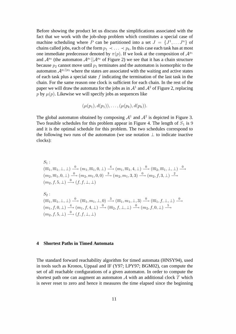
Before showing the product let us discuss the simplifications associated with thefact that we work with the job-shop problem which constitutes a special case ofmachine scheduling where P can be partitioned into a set J = {J 1, . . . Jn} ofchains called jobs, each of the form p1 ≺ . . . ≺ pk. In this case each task has at mostone immediate predecessor denoted by π(p). If we look at the composition of Ap1

and Ap2 (the automaton Ap1 ||Ap2 of Figure 2) we see that it has a chain structurebecause p2 cannot move until p1 terminates and the automaton is isomorphic to theautomaton Ap1||p2 where the states are associated with the waiting and active statesof each task plus a special state f indicating the termination of the last task in thechain. For the same reason one clock is sufficient for each chain. In the rest of thepaper we will draw the automata for the jobs as in A1 and A2 of Figure 2, replacingp by µ(p). Likewise we will specify jobs as sequences like

(µ(p1), d(p1)), . . . , (µ(pk), d(pk)).

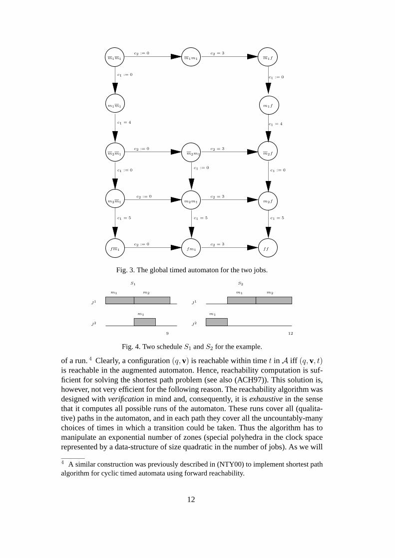
The global automaton obtained by composing A1 and A2 is depicted in Figure 3.Two feasible schedules for this problem appear in Figure 4. The length of S1 is 9and it is the optimal schedule for this problem. The two schedules correspond tothe following two runs of the automaton (we use notation ⊥ to indicate inactiveclocks):

S1 :

(m1,m1,⊥,⊥)0

−→ (m1,m1, 0,⊥)4

−→ (m1,m1, 4,⊥)0

−→ (m2,m1,⊥,⊥)0

−→

(m2,m1, 0,⊥)0

−→ (m2,m1, 0, 0)3

−→ (m2,m1, 3, 3)0

−→ (m2, f, 3,⊥)2

−→

(m2, f, 5,⊥)0

−→ (f, f,⊥,⊥)

S2 :

(m1,m1,⊥,⊥)0

−→ (m1,m1,⊥, 0)3

−→ (m1,m1,⊥, 3)0

−→ (m1, f,⊥,⊥)0

−→

(m1, f, 0,⊥)4

−→ (m1, f, 4,⊥)0

−→ (m2, f,⊥,⊥)0

−→ (m2, f, 0,⊥)5

−→

(m2, f, 5,⊥)0

−→ (f, f,⊥,⊥)

4 Shortest Paths in Timed Automata

The standard forward reachability algorithm for timed automata (HNSY94), usedin tools such as Kronos, Uppaal and IF (Y97; LPY97; BGM02), can compute theset of all reachable configurations of a given automaton. In order to compute theshortest path one can augment an automaton A with an additional clock T whichis never reset to zero and hence it measures the time elapsed since the beginning

11

m1m1m1m1 m1f

m2m1

m2m1

c1 = 4

c1 := 0

c1 := 0

m2m1

c1 := 0

c1 = 4

c1 := 0

c1 = 5

c2 = 3c2 := 0

c2 = 3c2 := 0

c2 = 3c2 := 0

c2 = 3c2 := 0

c1 := 0

c1 = 5 c1 = 5

fm1 ff

m2f

m2m1 m2f

m1fm1m1

fm1

Fig. 3. The global timed automaton for the two jobs.

9

m1

m2

J1

J2

S1

m1

12

m1

m1

m2

J1

J2

S2

Fig. 4. Two schedule S1 and S2 for the example.

of a run. 4 Clearly, a configuration (q, v) is reachable within time t in A iff (q, v, t)is reachable in the augmented automaton. Hence, reachability computation is suf-ficient for solving the shortest path problem (see also (ACH97)). This solution is,however, not very efficient for the following reason. The reachability algorithm wasdesigned with verification in mind and, consequently, it is exhaustive in the sensethat it computes all possible runs of the automaton. These runs cover all (qualita-tive) paths in the automaton, and in each path they cover all the uncountably-manychoices of times in which a transition could be taken. Thus the algorithm has tomanipulate an exponential number of zones (special polyhedra in the clock spacerepresented by a data-structure of size quadratic in the number of jobs). As we will

4 A similar construction was previously described in (NTY00) to implement shortest pathalgorithm for cyclic timed automata using forward reachability.

12

S′

m1 m2

m2

m1

m1

m1 m2

m1 m2

m1

S

J1

J2

J3

. . .

m1 m2

m1

S

m1

m2

Fig. 5. Removing laziness from a schedule S: first we eliminate laziness in the task ofJ2 which uses m1. This creates further manifestation of laziness which are subsequentlyremoved until a non-lazy schedule S is obtained. The dashed line indicates the frontierbetween L(S) and the rest of the tasks.

see, in our case, a much more efficient algorithm is possible.

We start with an observation concerning optimal schedules that we use to eliminatethe need for zones. A task p is enabled at time t in a given schedule if t ∈ [t1, t2]where t1 = en(π(p)), t2 = st(p) and the machine µ(p) is not used by any othertask. We say that a schedule S exhibits laziness at task p if p is enabled in a non-empty interval [t, st(p)]. A schedule is lazy if it exhibits laziness at one or moretask. We have noted before that sometimes it is preferable not to start a task as soonas it is enabled, however, this waiting is useless if no other task takes advantage ofit. 5 This fundamental intuition is formalized below.

Claim 1 (Non-Lazy Optimal Schedules) Any lazy schedule S can be transformedinto a non-lazy schedule S with |S| ≤ |S|. Hence every machine scheduling prob-lem admits an optimal non-lazy schedule.

Proof: The proof is by taking a lazy schedule S and transforming it into a scheduleS ′ in which laziness occurs “later”. A schedule induces a partial order relation@ on P defined as p @ p′ if either p ≺ p′ (when they belong to the same job)or µ(p) = µ(p′) and st(p) < st(p′) (when they are in conflict and the schedulegives priority to p). The laziness elimination procedure picks a lazy task p whichis minimal with respect to @ and shifts its start time backwards to the beginningof the laziness interval to yield a new feasible schedule S ′, such that |S ′| ≤ |S|.Moreover, the partial order associated with S ′ is identical to the one induced byS. The laziness at p is thus eliminated, and this might create new manifestations oflaziness at later tasks which are eliminated in the subsequent stages of the procedure(see illustration in Figure 5). Let L(S) = {p : ∃p′ v p s.t. there is laziness in p′},namely the set of tasks that are lazy or preceded by laziness. Clearly the lazinessremoval procedure decreases L(S) and terminates due to finiteness. 2

The next step is to restrict the runs of the automaton to those that correspond to

5 The situation is quite different in scheduling under uncertainty where waiting may leadto gaining additional information.

13

m1 m2

J1

J2

m3

Fig. 6. A lazy schedule which corresponds to an immediate run.

non-lazy schedules. A lazy run in a job-shop automaton A is a run containing afragment

(q, v) . . .t

−→ . . . (q′, v′)starti−→ (q′′, v′′)

such that the starti transition is enabled in all states (q, v), . . . , (q′, v′). As one cansee this notion is non local in the sense that at the moment of not taking the starti

transition we do not know yet whether this run will be extended to a lazy one. Tosimplify the presentation we will use here the weaker notion of an immediate run.The actual implementation generates only non-lazy runs and the reader can findmore details in (A02).

Definition 6 (Immediate Runs) An immediate run is a run in which whenever astart transition is taken in a state, it is taken as soon as it is enabled. A non-immediate run contains a fragment

(q, v)t

−→ (q, v + t)starti−→ (q′, v′).

Note that enabledness of start transitions does not depend on clock values. Clearlya schedule derived from a non-immediate run exhibits laziness, hence in order tofind an optimal schedule it is sufficient to explore the (finite) set of immediate runs.The converse is not true: Figure 6 shows a lazy schedule which is immediate. It islazy because m3 could have started at time 0, but it corresponds to an immediaterun because m3 was started after the termination of m1, that is, in a state differentfrom the state where it could have been started.

The restriction to immediate runs transforms the timed automaton into a discretedirected graph where nodes correspond to single configurations connected by asimple successor relation defined as follows. Let θ be the maximal amount of timethat can elapse in a configuration (q, v, t) until an end transition becomes enabled,i.e.

θ = min{(d(pi) − vi) : ci is active at q}.

The timed successor of a configuration is the result of letting time progress by θand terminating all that can terminate by that time:

Succt(q1, . . . , qn, v1, . . . , vn, t) = {(q′1, . . . , q′n, v′

1, . . . , v′n, t + θ)}

14

(⊥, 0, 0)

(⊥, ⊥, 3)

(0, ⊥, 3)

(⊥, ⊥, 4)

(0, ⊥, 4)

(0, ⊥, 0)

(⊥, ⊥, 0)

(⊥, 0, 4)

(⊥,⊥, 12)

(0, ⊥, 7)

(⊥, ⊥, 7)

(⊥, ⊥, 12)

(3, ⊥, 7)

(0, 0, 4)

(⊥, ⊥, 9)

(⊥, 0, 9)

(⊥, ⊥, 9)

f m1

f m1

m1 m1

m2 fm2 f

m2 m1

f ff f

m1 m1

m1 f

m1 f

m2 f

f f

m2 m1

m2 m1

m1 m1

m2 m1

Fig. 7. The immediate runs of the timed automaton of Figure 3

such that for every i

(q′i, v′i) =

(q′′i , v′′i ) if the transition (qi, vi + θ)

endi−→ (q′′i , v′′i ) is enabled

(qi, vi + θ) otherwise.

The discrete successors are all the successors by immediate start transition:

Succδ(q, v, t) = {(q′, v′, t) s.t. ∃i (q, v, t)starti−→ (q′, v′, t)}

The set of successors of each (q, v, t) is:

Succ(q, v, t) = Succt(q, v, t) ∪ Succδ(q, v, t).

Figure 7 shows the graph thus obtained from the automaton of Figure 3, wherethe paths correspond to the 5 immediate runs. Note that due to interleaving thesame schedule can be represented by more than one run. Applying standard searchalgorithms to this graph we can find the shortest path (and the optimal schedule)without using zone technology.

Although using points instead of zones reduces significantly the computationalcost, the inherent combinatorial explosion remains. In the rest of this section we de-scribe further methods to reduce the search space, some of which preserve the opti-

15

mal solutions and some provide sub-optimal ones. Similar ideas were first exploredin (BFH+01a). The first self-evident idea is to avoid exploring identical nodes ornodes that are obviously worse than nodes already explored.

Definition 7 (Domination) Let (q, v, t) and (q, v′, t′) be two reachable configura-tions. We say that (q, v, t) dominates (q, v′, t′) if t′ ≤ t and v ≥ v′.

Clearly if (q, v, t) dominates (q, v′, t′) then for every complete run going through(q, v′, t′) there is a run through (q, v, t) which is not longer. Hence whenever weencounter a new node in the graph we check whether it is dominated by an exploredor waiting node and in this case we discard it. If it dominates a node in the waitinglist we replace it.

The next thing to do is to apply best-first search and explore the “most promising”nodes first. To this end we need an evaluation function over configurations. Con-sider a job J = (p1, d1), . . . (pk, dk) and its corresponding automaton. For everyconfiguration (q, v) of this automaton g(q, v) is a lower-bound on the time remain-ing until f is reached from the configuration (q, v):

g(f,⊥) = 0

g(pj,⊥) =∑k

l=j d(pl)

g(pj , v) = g(pj,⊥) − v

The evaluation of global configurations is defined as:

E((q1, . . . , qn), (v1, . . . , vn, t)) = t + max{g(qi, vi)}ni=1

Note that max{g} gives the most optimistic estimation of the remaining time tocompletion, assuming that no job will have to wait due to a conflict. The best-first search algorithm below maintains the waiting list sorted according to E . It isguaranteed to produce the optimal path because it stops the exploration only whenit is clear that the unexplored states cannot lead to schedules better than those foundso far.

Algorithm 1 (Best-first Forward Reachability)

16

Waiting:={Succ(s, 0, 0)};Best:=∞(q, v, t):= first in Waiting;while E(q, v, t) < BestdoFor every (q′, v′, t′) ∈ Succ(q, v, t);

if q′ = f thenBest:=min{Best, t′}

elseInsert (q′, v′, t′) into Waiting;

Remove (q, v, t) from Waiting(q, v, t):= first in Waiting;

end

A prototype implementation of this algorithm can find optimal schedules for prob-lems with up to 6 jobs and 6 machines in few seconds. To treat larger problems weresort to a heuristic algorithm which is not guaranteed to produce the optimal so-lution. The algorithm is a mixture of breadth-first and best-first search with a fixednumber w of explored nodes at any level of the automaton. For every level we takethe w best (according to E) nodes, generate their successors but explore only thebest w among them, and so on. The number w is the main parameter of this tech-nique, and although the number of explored states grows monotonically with w, thequality of the solution does not — sometimes the solution found with a small w isbetter than the one found with a larger one.

We tested the heuristic algorithm on 10 problems among the most notorious job-shop scheduling problems. Note that these are pathological problems with a largevariability in step durations, constructed to demonstrate the hardness of job-shopscheduling. For each of these problems we have applied our algorithm for differentchoices of w. In Table 1 we compare our best results on these problems with thebest results reported in Table 15 of the comprehensive survey (JM99), where theresults of the 18 best-known methods were compared. As one can see our resultsare typically 5−10% longer than the optimum. For comparison, an algorithm whichpicks the best out of 3000 randomly generated runs deviates from the optimum bymore than 100%.

5 Scheduling under Uncertainty

The problem treated so far was completely deterministic. All the information con-cerning the tasks to be executed was known in advance, including their identity,inter-dependence, duration and release time. The same goes for the machines whosequantity was assumed to be fixed. Real life is not like that. New tasks can arrive in

17

problem heuristic Opt

name #j #m time length deviation length

FT10 10 10 3 969 4.09 % 930LA02 10 5 1 655 0.00 % 655LA19 10 10 15 869 3.21 % 842LA21 10 15 98 1091 4.03 % 1046LA24 10 15 103 973 3.95 % 936LA25 10 15 148 1030 5.42 % 977LA27 10 20 300 1319 6.80 % 1235LA29 10 20 149 1259 9.29 % 1152LA36 15 15 188 1346 6.15 % 1268LA37 15 15 214 1478 5.80 % 1397

Table 1The results for 10 hard problems using the bounded width heuristic. The first three columnsgive the problem name, number of jobs and number of machines (and tasks). Our results(time in seconds, the length of the best schedule found and its deviation from the optimum)appear next.

the middle of execution while others can be canceled. Task processing can takemore or less time than expected, machines may break down, cost criteria maychange, etc. In such situations the actual evolution of the system depends on theactions of two “players”, the scheduler which decides whether or not to start atask in a given situation and the “environment”, a generic name for all sources ofuncontrolled external events such as the arrival or termination of a task.

5.1 Strategies and their Evaluation

The evaluation or optimization of the performance of such an open reactive sys-tem which interacts with an external environment, raises some serious conceptualproblems. 6 In a deterministic setting, each scheduler induces a unique scheduleaccording to which it can be evaluated and compared with other candidate sched-ulers. For an open system S, each instance d of the environment can potentiallyinduce a different behavior S(d), and the question is how to take all these behav-iors into account while evaluating and comparing schedulers. Several approachesto this problem are commonly used:

• Worst-case: The system is evaluated according to its worst behavior.• Average-case: The set of all environment instances is considered as a probability

space and this induces a probability over all system behaviors. The system isthen evaluated according to the expected value (over all its behaviors) of theperformance measure.

6 Readers interested in a more comprehensive discussion of these issues are invited to lookat (M04).

18

• Nominal-case: The system is evaluated based on one behavior which correspondsto one “typical” instance of the environment.

Each of these approaches has its advantages and shortcomings. The worst-case ap-proach is often used for safety-critical systems where the cost associated with badbehaviors is too high to tolerate, even if they constitute a negligible fraction of thepossible behaviors. This is implicitly the approach taken in verification, where theperformance measure is discrete and consists of a binary classification into “cor-rect” and “incorrect”, and this means that a system is correct only if all its behav-iors satisfy the property in question. On the negative side, this approach might leadto an over-pessimistic allocation of resources which can be very inefficient duringmost of the system lifetime. 7

The probabilistic approach is more appropriate when the performance measure ismore “continuous” in nature, e.g. the waiting time in a queue, and one can toler-ate some performance degradation during pressure periods. The implicit assump-tion underlying the nominal approach is somewhat similar to the probabilistic one,namely, the nominal behavior is “close” to most of the behaviors we are likely tosee during the system life-time and the performance of other behaviors varies “con-tinuously” with the distance from the nominal one. This approach is widely (andimplicitly) used in Control Theory, for example, in “step response” analysis thesystem is simulated with one disturbance which is, in certain cases, sufficient forits evaluation.

From a computational standpoint the evaluation of a given scheduler S is the easiestunder the nominal approach because when d is fixed the system is closed and thebehavior S(d) can be computed by simple simulation (it is represented by a singlepath in the corresponding automaton). Moreover, the comparison of two candidatesystems S and S ′ is based on the same d. In the worst-case approach when it is notknown a-priori which d induces the worst behavior, one has to “simulate exhaus-tively” and evaluate the scheduler against all instances in order to find the worst-case. This is the inherent difficulty of verification compared to testing/simulation.Moreover, when we want to compare S and S ′ for optimality, it might be that eachof them attains its worst performance on a different instance. The probabilistic ap-proach is a-priori 8 the most difficult because not only do we need to explore allbehaviors but also to keep track of their probabilities in order to compute the overallevaluation of the system.

7 A good analogy is to live all your life wearing a helmet fearing a meteorite rain, or goingto the airport a day before the flight in anticipation of all conceivable traffic jams.8 At least when the approach is applied naively without using additional mathematicalinformation that can lead to analytic solutions in some special cases.

19

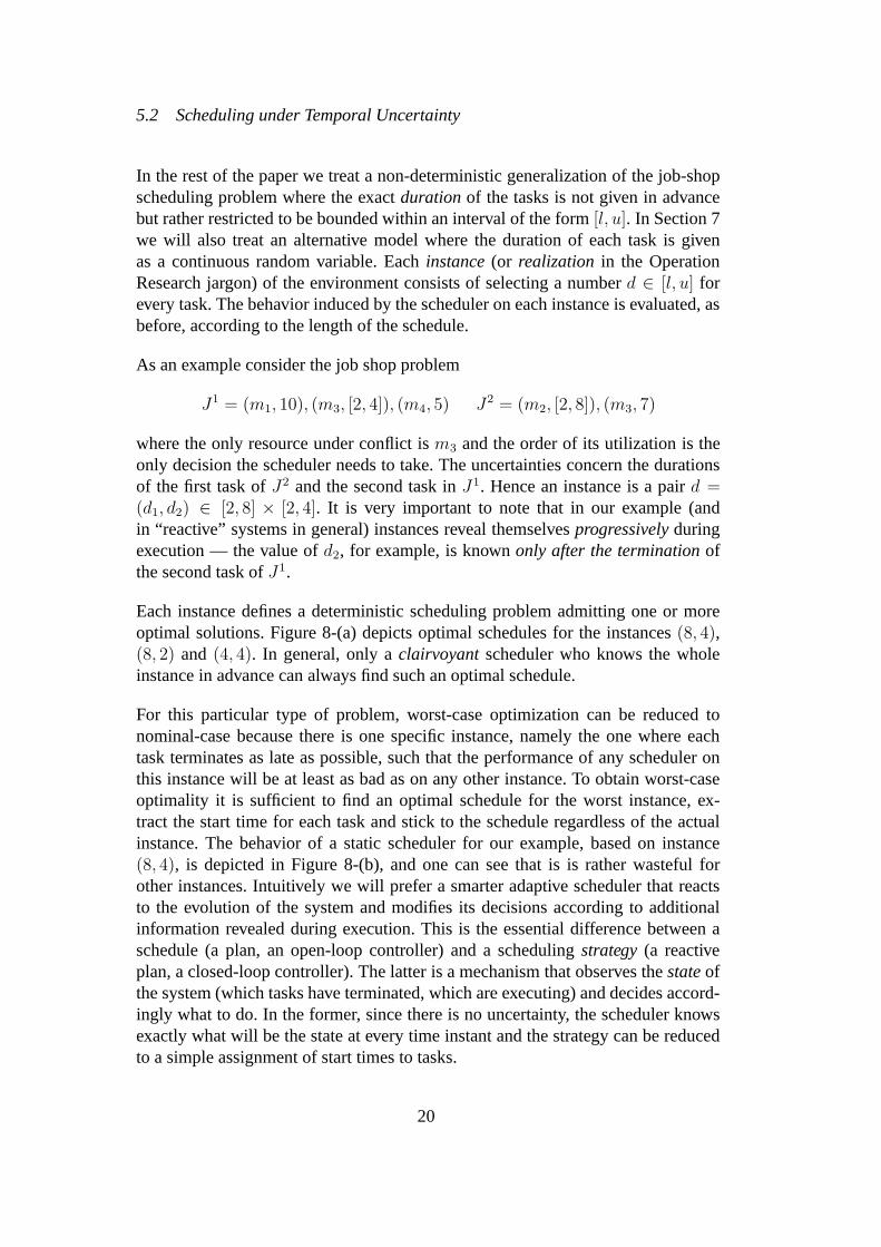
5.2 Scheduling under Temporal Uncertainty

In the rest of the paper we treat a non-deterministic generalization of the job-shopscheduling problem where the exact duration of the tasks is not given in advancebut rather restricted to be bounded within an interval of the form [l, u]. In Section 7we will also treat an alternative model where the duration of each task is givenas a continuous random variable. Each instance (or realization in the OperationResearch jargon) of the environment consists of selecting a number d ∈ [l, u] forevery task. The behavior induced by the scheduler on each instance is evaluated, asbefore, according to the length of the schedule.

As an example consider the job shop problem

J1 = (m1, 10), (m3, [2, 4]), (m4, 5) J2 = (m2, [2, 8]), (m3, 7)

where the only resource under conflict is m3 and the order of its utilization is theonly decision the scheduler needs to take. The uncertainties concern the durationsof the first task of J2 and the second task in J1. Hence an instance is a pair d =(d1, d2) ∈ [2, 8] × [2, 4]. It is very important to note that in our example (andin “reactive” systems in general) instances reveal themselves progressively duringexecution — the value of d2, for example, is known only after the termination ofthe second task of J1.

Each instance defines a deterministic scheduling problem admitting one or moreoptimal solutions. Figure 8-(a) depicts optimal schedules for the instances (8, 4),(8, 2) and (4, 4). In general, only a clairvoyant scheduler who knows the wholeinstance in advance can always find such an optimal schedule.

For this particular type of problem, worst-case optimization can be reduced tonominal-case because there is one specific instance, namely the one where eachtask terminates as late as possible, such that the performance of any scheduler onthis instance will be at least as bad as on any other instance. To obtain worst-caseoptimality it is sufficient to find an optimal schedule for the worst instance, ex-tract the start time for each task and stick to the schedule regardless of the actualinstance. The behavior of a static scheduler for our example, based on instance(8, 4), is depicted in Figure 8-(b), and one can see that is is rather wasteful forother instances. Intuitively we will prefer a smarter adaptive scheduler that reactsto the evolution of the system and modifies its decisions according to additionalinformation revealed during execution. This is the essential difference between aschedule (a plan, an open-loop controller) and a scheduling strategy (a reactiveplan, a closed-loop controller). The latter is a mechanism that observes the state ofthe system (which tasks have terminated, which are executing) and decides accord-ingly what to do. In the former, since there is no uncertainty, the scheduler knowsexactly what will be the state at every time instant and the strategy can be reducedto a simple assignment of start times to tasks.

20

m1

m2

m4m3

m3

20

m3 m4

m3

19

m3

21

J1

J2

J2

J1

J1

J2

(4, 4)

(8, 2)

(8, 4) m2

m1

m1

m2

m4m3

m1

m2 m3

m1

m2

m3 m4

m3

m4m3

m1 m4

m2 m3

m3

21

21

21

(a) (b)

(8, 2)

(8, 4)

J2

J1

J2

J2

J1

J1

(4, 4)

m1

m1

m2

m3

19

m4m3

m3

m4

m3

m1 m4

m2 m3

m3

m2

21

21

m1

m2

m4m3

m3

m3m2

m1 m4m3

21

21

(c) (d)

Fig. 8. (a) Optimal schedules for three instances. For the first two the optimum is obtainedwith J1

@ J2 on m3 while for the third — with J2@ J1; (b) A static schedule based on the

worst instance (8, 4). It gives the same length for all instances; (c) The behavior of a holefilling strategy based on instance (8, 4); (d) The equal performance of the two strategies oninstance (5, 4).

One of the simplest ways to be adaptive is the following. First we choose a nominalinstance d and find a schedule S which is optimal for that instance. Rather thantaking S “literally” as the function st, we extract from it only the qualitative in-formation, namely the order in which conflicting tasks utilize each resource. In ourexample the optimal schedule for the worst instance (8, 4) is associated with theordering J1

@ J2 on m3. Then, during execution, we start every task as soon as itspredecessors have terminated, provided that the ordering is not violated (a similarstrategy was used in (NY01) and probably elsewhere). As Figure 8-(c) shows, sucha strategy is better than the static schedule for instances such as (8, 2) where it takesadvantage of the earlier termination of the second task of J 1 and “shifts forward”the start times of the two tasks that follow. On the other hand, instance (4, 4) can-not benefit from the early termination of m2 because shifting m3 of J2 forward willviolate the J1

@ J2 ordering on m3.

Note that this “hole-filling” strategy is not restricted to the worst-case. One can useany nominal instance and then shift tasks forward or backward in time as needed

21

while maintaining the order. On the other hand, a static schedule (at least wheninterpreted as a function from time to actions) can only be based on the worst-case— a schedule based on another nominal instance may assume a resource availableat some time point, while in reality that resource will be occupied.

While the hole filling strategy can be shown to be optimal for all those instanceswhose optimal schedule has the same ordering as that for the nominal instance, itis not good for instances such as (4, 4) where a more radical form of adaptivenessis required. If we look at the optimal schedules for (8, 4) and (4, 4) (Figure 8-(a))we see that in both of them the decision whether or not to give m3 to J2 is taken atthe same qualitative state where m1 is executing and m2 has terminated. The onlydifference is in the elapsed execution time of m1 at the decision point. Hence anadaptive scheduler should base its decisions also on such quantitative informationwhich, in the case of timed automaton models, is represented by clock values.

Consider the following approach: initially we find an optimal schedule for somenominal instance. During execution, whenever a task terminates (before or after thetime it was assumed to) we reschedule the “residual” problem, assuming nominalvalues for the tasks that have not yet terminated. In our example, we first build anoptimal schedule for (8, 4) and start executing it. If task m2 in J2 terminated after4 time units we obtain the residual problem

J ′1 = (m1,6), (m3, 4), (m4, 5) J ′

2 = (m3, 7)

where the boldface letters indicate that m1 must be scheduled immediately (it isalready executing and we assume no preemption). For this problem the optimalsolution will be to give m3 to J2. Likewise if m2 terminates at 8 we have

J ′1 = (m1,2), (m3, 4), (m4, 5) J ′

2 = (m3, 7)

and the optimal schedule consists of waiting for the termination of m1 and thengiving m3 to J1. The property of the schedules obtained this way, is that at anymoment in the execution they are optimal with respect to the nominal assumptionconcerning the future. 9

This approach involves a lot of online computation, namely solving a new schedul-ing problem each time a task terminates. The alternative approach that we proposeis based on expressing the scheduling problem using timed automata and synthesiz-ing a controller off-line. In this framework (AMPS98; AM99; AGP99) a strategyis a function from states and clock valuations to controller actions (in this casestarting tasks). After computing such a strategy and representing it properly, theexecution of the schedule may proceed while keeping track of the state of the cor-responding automaton. Whenever a task terminates, the optimal action is retrieved

9 A similar idea is used in model-predictive control where at each time actions at thecurrent “real” state are re-optimized while assuming some nominal prediction of the future.

22

from the strategy look-up table and the results are identical to those obtained viaonline re-scheduling. 10 The major contribution of this paper is the formalization ofthis intuition and the development and implementation of an algorithm for findingadaptive schedulers that are optimal in this sense.

5.3 Problem Statement

Definition 8 (Uncertain Machine Scheduling)An uncertain machine scheduling problem is J = (P,≺,M, µ,D, U) where P ,≺, M and µ are as in Definition 1, D : P → Int(N) assigns an integer-boundedinterval to each task and U ⊆ P is a subset of immediate tasks consisting of some≺-minimal elements.

The set U is typically empty in the initial definition of the problem and we need itto define residual problems. We use Dl and Du to denote the projection of D onthe lower- and upper-bounds of the interval, respectively.

An instance of the environment is any function d : P → R+, such that d(p) ∈ D(p)for every p ∈ P . The set of instances admits a natural partial-order relation: d ≤ d′

if d(p) ≤ d′(p) for every p ∈ P . Any environment instance induces naturally adeterministic instance of J , denoted by J (d). The worst-case is defined by themaximal instance d where d(p) = Du(p) for every p.

A feasible schedule for an instance J (d) of the problem is characterized, as inDefinition 2, by a function st : P → R+ denoting the start time of each task,satisfying the precedence and mutual exclusion constraint, as well as the additionalcontinuity constraint stating that st(p) = 0 for every p ∈ U .

In order to be adaptive we need a scheduling strategy, a rule that may induce adifferent schedule for each d. However, this definition is not simple because weneed to restrict ourselves to causal strategies, strategies that can base their decisionsonly on information available at the time they are made. In our case, the actualvalue of d(p) is revealed only when p terminates.

Definition 9 (State of Schedule)A state of a schedule S at time t is s = (P f , P a, κ, P e) such that P f is a downward-closed subset of (P,≺) consisting of tasks that have terminated (those satisfyingen(p) ≤ t) , P a is a set of active tasks currently being executed (those satisfyingst(p) ≤ t < en(p)), κ : P a → R+ is a function such that κ(p) = t−st(p) indicatesthe time elapsed since the activation of p and P e is the set of enabled tasks, those

10 Of course, there is a trade-off between what we gain by reducing online computation timeand what we pay in terms of offline computation time and in terms of the space needed tostore the strategy.

23

whose predecessors are in P f . The set of all possible states is denoted by S .

Definition 10 (Scheduling Strategy) A (state-based) scheduling strategy is a func-tion σ : S → P ∪ {⊥} such that for every s = (P f , P a, c, P e), σ(s) ∈ P e ∪ {⊥}and if σ(s) = p then µ(p) 6= µ(p′) for every p′ ∈ P a.

In other words, a strategy decides at each state whether to do nothing and wait forthe next event (⊥) or to start executing an enabled task which is not in conflict withany active task. An operational definition of the interaction between a strategy andan instance will be given later using timed automata, but intuitively one can see thatthe evolution of the schedule consists of time passage interleaved with two typesof transitions: uncontrolled transitions where an active task p terminates after d(p)time and moves from P a to P f (leading possibly to the insertion of new tasks toP e) and a decision of the scheduler to start an enabled task. The combination of astrategy and an instance yields a unique schedule S(d, σ) and we say that a state is(d, σ)-reachable if it occurs in S(d, σ).

Remark: In certain types of games, the optimal strategy may be history-dependent,that is, it will make different decisions at the same state depending on the paththrough which it has been reached. However in games like those considered in thepaper where the cost function is additive, it can be shown that state-strategies (alsoknown as positional strategies in Game Theory) are sufficient for optimality.

Next we formalize the notion of a residual problem, namely a specification of whatremains to be done in an intermediate state of the execution. We use a −. b formax{0, a − b} and [a, b] −. c for [a −. c, b −. c].

Definition 11 (Residual Problem) Let s = (P f , P a, κ, P e) be a state of a sched-ule for the problem J = (P,M,≺, µ,D, U). The residual problem starting from sis Js = (P − P f ,M,≺′, µ′, D′, P a) where ≺′ and µ′ are, respectively, the restric-tions of ≺ and µ, to P − P f and D′ is constructed from D by letting

D′(p) =

{

D(p) −. κ(p) if p ∈ P a

D(p) otherwise

Likewise a residual instance ds is the instance d restricted to P − P f defined as

ds(p) =

{

d(p) −. κ(p) if p ∈ P a

d(p) otherwise

Let d be an instance. A strategy σ is d-future-optimal if for every instance d′ andfrom every (σ, d′)-reachable state s, it produces the optimal schedule for the resid-ual problem Js(ds). If we take d to be the maximal instance, this is exactly theproperty of the online re-scheduling approach described informally in the previoussection.

24

6 Optimal Strategies for Timed Automata

In this section we show how the problem of finding d-future optimal strategies canbe formulated and solved algorithmically using timed automata. The algorithm willbe presented in two levels of abstraction. At the higher level, we present a dynamicprogramming algorithm that computes iteratively a value function defined on thestate space of the timed automaton. This is the cost-to-go function denoting thelength of the shortest path to termination from each configuration. At the moreconcrete level we explain how this function is represented and computed usinga slight modification of the standard backward reachability algorithm for timedautomata.

6.1 Modeling

The modeling of the problem with timed automata is similar to Definition 4 withmore attention paid to the distinction between controlled and uncontrolled transi-tions. The automaton Ap

D of Figure 9 models all the possible (isolated) behaviorsof a task p with D(p) = [l, u]. The start transition is controlled and can be ini-tiated by the scheduler any time, given that precedence constraints are met. Theend transition is initiated by the environment and can be taken within t ∈ [l, u]time after start. This uncertainty is modeled using the staying condition c ≤ ufor state p and the transition guard c ≥ l. 11 Composing these automata, as in thedeterministic case, gives a global automaton AD, such that the set of its runs coversall the schedules that are feasible under all possible combinations of strategies andinstances.

As a running example consider a simplified version of the example of Section 5with only one uncertain duration:

J1 = (m1, 10), (m3, , 4), (m4, 5) J2 = (m2, [2, 8]), (m3, 7).

The automata for the example and their composition appear in Figure 10. The cor-respondence between schedule states and reachable configurations is straightfor-ward. Moreover, the residual problem associated with any state of the schedule isrepresented by the sub-automaton rooted in the corresponding configuration.

The automaton can be viewed as specifying a game between the scheduler and theenvironment. The environment can decide whether or not to take an end transitionand terminate an active task, and the scheduler can decide whether or not to takesome enabled start transition. A state-based strategy is a function that maps any

11 An elegant alternative to using staying condition could be to use timed automata withdeadlines (SY96) which are rich enough to express our scheduling problems.

25

φ1φ1/c := 0

c ≤ d

c ≥ d

p

p

p

Ap

d

φ1/c := 0

c ≤ u

p

p

p

c ≥ d

Ap

D,d

φ1/c := 0

c ≤ u

c ≥ l

p

p

p

Ap

D

p

p

p

λ

Ap

λ

startstart startstart

end endend end

Fig. 9. The generic automaton ApD for a task p such that D(p) = [l, u]. The automaton Ap

d

for a deterministic instance d. The automaton ApD,d for computing d-future optimal strate-

gies and the automaton Apλ for an exponentially distributed duration. Staying conditions for

p and p are true and are omitted from the figure.

configuration of the automaton either into one of its transition successors or to thewaiting “action”. For example, at (m1,m3) there is a choice between moving to(m1,m3) by giving m3 to J2 or waiting until J1 terminates m1 and letting theenvironment take the automaton to (m3,m3). Such decisions, as we shall see, maydepend also on clock values.

Let Σ be the set of starti transitions and let Σq denote those transitions that areenabled at global state q of the automaton. A scheduling strategy is a partial func-tion σ : Q × V → Σ ∪ {⊥} such that σ(q, v) ∈ Σq ∪ {⊥}, which is defined atleast for every state which is (d, σ)-reachable for some instance d. Let Vi(q) = {v :σ(q, v) = starti} denote the clock values at which the strategy decides to start taskpi at q, and let V⊥(q) = {v : σ(q, v) = ⊥} be the values at which it decides to wait.Synthesizing the strategy can be seen as eliminating from the automaton the non-determinism on the scheduler side by restricting the guards and staying conditionsuch that at any configuration only one transition guard or staying condition holds.

Definition 12 (Strategy Automaton) Let AD be the automaton describing an un-certain scheduling problem and let σ : Q × V → Σ ∪ {⊥} be a strategy. The au-tomaton Aσ

D, obtained from AD by restricting the transition guards of every state qto Vi(q) and intersecting the staying condition with V⊥(q).

Note that a-priori the sets Vi(q) and V⊥(q) could have complicated forms which gooutside the expressive power of timed automata, but as we shall see (and as was thecase in (MPS95; AM99)), for optimal strategies these sets can be expressed usingzones. A strategy σ is d-future optimal if from every configuration reachable in Aσ

D,it gives the shortest path to the final state (assuming that the remaining uncontrolledtransitions are taken according to d). In the sequel we use a simplified form of thedefinitions and the algorithm of (AM99) to find such strategies.

26

m3m2

m4m2

m1m2

fm2

m1m2

m1m2

m3m2

m1m2

m3m2

m4m2

m4m2

fm2

m1m2

m3m2

m1m3

m3m3

m3m3

m4m3

m4m3

m1m3

m1m3

m3m3

m4m3

fm3fm3

m1m3 m1f

m1f

m3f

m3f

m4f

m4f

ff

c2 ≥ 2

c2 ≥ 2

c2 ≥ 2

c2 ≥ 2

c2 ≥ 2

c2 ≥ 2

c2 ≥ 2

c1 := 0

c1 = 10

c1 := 0

c1 = 4

c1 := 0

c1 = 5

c1 := 0

c1 = 10

c1 := 0

c1 = 4

c1 := 0

c1 = 5

c1 := 0

c1 = 10

c1 := 0

c1 = 4

c1 := 0

c1 = 5

c1 := 0

c1 = 5

c1 = 10

c1 := 0c1 := 0

c2 := 0

c2 := 0

c2 := 0

c2 := 0

c2 := 0

c2 := 0

c2 := 0 c2 := 0

c2 := 0

c2 := 0

c2 := 0

c2 := 0

c2 := 0 c2 = 7

c2 = 7

c2 = 7

m4m3

c2 = 7

c2 = 7

c2 = 7

c1 = 10

c1 := 0

c1 = 4

c1 := 0

c1 = 5

c2 := 0 c2 := 0 c2 = 7c2 ≥ 2

m3 f

m1

m1

m3

m4

f

c1 = 10

c1 := 0

c1 := 0

c1 = 4

c1 := 0

c1 = 5

m3

m2 m3

m4

m2

c2 ≤ 8

c2 ≤ 8

c2 ≤ 8

c2 ≤ 8

c2 ≤ 8

c2 ≤ 8

c2 ≤ 8

c2 ≤ 8

Fig. 10. The global automaton for the job-shop specification. The automata on the left andupper parts of the figure are those of the two jobs.

6.2 The Value Function and Abstract Algorithm

The particularity of d-future optimal strategies where the “current” state (where adecision should be taken) could have been reached by any choice of duration by theenvironment, while the decision at that state is based on assuming d for the future,forces us to use a slightly modified automaton to do our computation. We will usethe automaton Ap

D,d of Figure 9 to model each task. It can terminate as soon as

27

c ≥ d but can stay in p until c = u. We denote by AD,d = (Q,C, I, ∆, s, f) theautomaton obtained by composing these automata.

The strategy is obtained as a side effect of computing the value function h : Q ×V → R+ where h(q, v) is the length of the minimal run from (q, v) to f , assumingthat all uncontrolled future transitions will be taken according to d. This functionsatisfies

h(q, v) = min{t + h(q′, v′) : (q, v)t

−→ (q, v + t1)0

−→ (q′, v′)}

In other words, to compute h(q, v) we should compare all the possibilities to staysome time t in q and then take a transition to some (q ′, v′). The Bellman principleguarantees that the value associated with such possibility is the sum of t plus thevalue of (q′, v′). Note that h can be written as

h(q, v) = min{hδ(q, v), h⊥(q, v)}

wherehδ(q, v) = min{h(q′, v′) : (q, v 0

−→ (q′, v′)}

is the value achieved by taking the best enabled transition immediately (non-laziness),and

h⊥(q, v) = t + h(q′, v′)

is the value associated with waiting, where t is the minimal distance from v to aguard of an uncontrolled transition to (q′, v′) while assuming instance d (recall thatthe guards in the automaton on which the computation is performed are of the formc ≥ d).

To understand how this works in our case consider a configuration (q0, v0) =(p1, p2, p3, p4, v1, v2,⊥,⊥) where two tasks are executing and two tasks are waiting(see Figure 11). Among the two uncontrolled end transitions only one can be taken,namely end1 if d1 − v1 < d2 − v2 or end2 otherwise. 12 Suppose that the first caseholds, and let t = d1−v1. The other transitions can be taken anytime between 0 andt but the non-laziness result, which still holds because we assume a deterministicd-future, tells us that if we take them, we should take them immediately. Hencein this case we have h(q0, v0) = min{d1 − v1 + h(q1, v1), h(q3, v3), h(q4, v4)}. Inanother configuration where d1−v1 > d2−v2 we should replace d1−v1+h(q1, v1)by d2−v2+h(q2, v2). Note that h should be defined also for clock valuations wherevi > di but still less than ui.

The abstract algorithm for computing h works iteratively by letting

h0(q, v) =

{

0 if q = f

∞ otherwise

12 We ignore here the case of equality when two uncontrolled transitions are enabled atexactly the same time. The special structure of our automata guarantees that such transitionscommute anyway.

28

q3, v3 q4, v4q2, v2

q0, v0

q1, v1

end1

c2 ≥ d2

end2

c3 := 0

start3

c4 := 0

start4

c1 ≥ d1

Fig. 11. Computing the value function.

and then

hk+1(q, v) = min({hk(q, v)}∪{t+hk(q′, v′) : (q, v)

t−→ (q, v+ t1)

0−→ (q′, v′)}),

until hk+1 = hk. The correctness of this procedure for the more general case ofarbitrary timed automata has been proved in (AM99). The proof is based on show-ing that hk(q, v) is the length of the shortest path (among those that have not morethan k transitions) from (q, v) to termination, and that the hk’s range over a classof “nice” functions closely related to the zones used in the verification of timed au-tomata. This class is well-founded and hence the computation of h terminates evenfor cyclic automata, a fact that we do not need here as h is computed in one sweepthrough all acyclic paths from the final to the initial state. Note that all such pathshave the same number of transitions.

After having computed h, the extraction of a strategy is straightforward: if the op-timum of h at (q, v) is obtained via a controlled starti transition we let σ(q, v) =starti, otherwise we let σ(q, v) = ⊥. In case when the optimum is obtained viamore than one continuation we can define some “tie breaking” rules which pre-fer, say, waiting over action, and start the task with the least index when there areseveral candidates.

Before presenting the more concrete version of the algorithm let us illustrate thecomputation of h on our example. We start with

h(f, f,⊥,⊥) = 0

h(m4, f, v1,⊥) = 5 −. v1

h(f,m3,⊥, v2) = 7 −. v2,

because the time to reach (f, f) from (m4, f) is the time it takes to satisfy the guardc1 = 5, etc. The value of h at (m4,m3) depends on the values of both clocks whichdetermine which of m3, m4 will terminate first and whether the shorter path goes

29

via (m4, f) or (f,m3).

h(m4,m3, v1, v2) = min

{

7 −. v2 + h(m4, f, v1 + 7 −. v2,⊥),

5 −. v1 + h(f,m3,⊥, v2 + 5 −. v1)

}

= min{5 −. v1, 7 −. v2}

=

{

5 −. v1 if v2 −. v1 ≥ 2

7 −. v2 if v2 −. v1 ≤ 2

Note that the corresponding transitions are both uncontrolled end transitions andno decision of the scheduler is required in this state.

This procedure goes higher and higher in the graph, computing h for the wholereachable state-space Q × V . In particular, for state (m1,m3) where we need todecide whether to give m3 to J2 or to wait, we obtain:

h(m1,m3, v1,⊥) = min{16, 21 −. v1}

=

{

16 if v1 ≤ 5

21 −. v1 if v1 ≥ 5

As for the strategy, one can see that at (m1,m3) the optimal result is obtained bygiving m3 immediately to J2 and moving to (m1,m3) when v1 ≤ 5 or by waiting tothe termination of m1, reaching (m3,m3) and then moving to (m3,m3) if v1 ≥ 5.Note that if we assume that J1 and J2 started their first tasks simultaneously, thevalue of c1 upon entering (m1,m3) is exactly the duration of m2 in the instance.Figure 8-(d) shows that, indeed, the two choices coincide in performance whenv1 = 5.

6.3 The Concrete Algorithm

We now describe how h is computed using a standard backward reachability algo-rithm that works on sets, not on functions. Let Θ be an upper bound on the lengthof the worst-case optimal schedule, for example the sum of the maximal durationsof all tasks. Instead of computing h directly we compute the set

R = {(q, v, t) : Θ − t ≥ h(q, v) ∧ t ≥ 0}.

Note, that R contains exactly the same information as h and, in particular, h can bereconstructed from R:

h(q, v) = min{Θ − t : (q, v, t) ∈ R}

30

Moreover, since h(q, v) ≤ Θ for any (q, v) which is forward reachable in AD, anysuch (q, v) is a projection of some point (q, v, t) ∈ R. Consequently, computing Ramounts to computing the strategy for every reachable configuration.

From the definitions of h and R, a triple (q, v, t) belongs to R iff one can reachthe final state (f,⊥) of the automaton from (q, v) within Θ − t time, assuminginstance d for all tasks that have not terminated in (q, v). Hence the set R can becharacterized in terms of reachability as follows. Let A′

D,d be the auxiliary automa-ton obtained by augmenting AD,d with a clock T which is never reset to zero (asin Section 4) and by adding the constraint T < Θ to the staying condition of everystate (to avoid divergence of T ). The following result gives a useful characterizationof R.

Lemma 1 A configuration (q, v, t) ∈ R iff the state (f,⊥, Θ)) is reachable from(q, v, t) in A′

D,d.

Proof: If there is a run in A′D,d, from (q, v, t) to (f,⊥, Θ), then, by the definition of

the auxiliary clock T , this run is of duration Θ − t and (q, v, t) ∈ R. Conversely, if(q, v, t) ∈ R, then there exists t′ ≥ t and a run of A′

D,d from (q, v, t′) to (f, ,⊥, Θ)of duration Θ− t′. By subtracting (t′− t) from T on both sides of the run we obtaina run from (q, v, t) to (f,⊥, Θ−(t′− t)) which can be extended, via idling for t′− ttime in f , into a run of length Θ − t. 2

Hence, the set R can be obtained by the standard backward reachability algorithmfor timed automata, and has a form of a finite union of zones. For completeness weinstantiate the backward reachability algorithm for this case.

We recall some commonly-used definitions in the verification of timed automata(HNSY94). A zone is a subset of V consisting of points satisfying a conjunctionof inequalities of the form ci − cj ≥ k or ci ≥ k. A symbolic state is a pair (q, Z)where q is a discrete state and Z is a zone. It denotes the set of configurations{(q, v) : v ∈ Z}. Zones and symbolic states are closed under various operationsincluding the following:

• The time predecessors of (q, Z) is the set of configurations from which (q, Z)can be reached by letting time progress:

Pret(q, Z) = {(q, v) : v + r1 ∈ Z, r ≥ 0}.

• The δ-transition predecessor of (q, Z) is the set of configurations from which(q, Z) is reachable by taking the transition δ = (q′, φ, ρ, q) ∈ ∆:

Preδ(q, Z) = {(q′, v′) : v′ ∈ Reset−1ρ (Z) ∩ φ ∩ Iq′}.

• The predecessors of (q, Z) is the set of all configuration from which (q, Z) is

31

reachable by any transition δ followed by passage of time:

Pre(q, Z) =⋃

δ∈∆

Preδ(Pret(q, Z)).

The result can be represented as a set of symbolic states.

Algorithm 2 is based on the standard backward reachability algorithm for timedautomata. It starts with the final state of A′ (with T = Θ) in a waiting list andoutputs the set R of all backward-reachable symbolic states. In order to be able toextract strategies we store tuples of the form (q, Z, q′) such that Z is a zone of A′

and q′ is the successor of q from which (q, Z) was reached backwards.

Algorithm 2 (Backward Reachability for Timed Automata)Waiting:={(f, {(⊥, Θ)}, ∅)};Explored:=∅;while Waiting 6= ∅ doPick (q, Z, q′′) ∈ Waiting;For every (q′, Z ′) ∈ Pre(q, Z);

Insert (q′, Z ′, q) into Waiting;Move (q, Z, q′′) from Waiting to Explored

endE:=Explored

The backward reachable set of states R is related to the set of triples E as follows:

(q, v, t) ∈ R ⇔ ∃Z, q′ : (v, t) ∈ Z ∧ (q, Z, q′) ∈ E.

For implementing the strategy it is convenient to use the set of triples E. Whenevera transition to (q, v) is taken during the execution we look at all the symbolic stateswith discrete state q and find by which tuple (q, Z, q′) the minimum

h(q, v) = min{Θ − t : (v, t) ∈ Z ∧ (q, Z, q′) ∈ E}

is obtained. If q′ is a successor via a controlled transition, we move to q ′, otherwisewe wait until a task terminates and an uncontrolled transition is taken. Non-lazinessguarantees that we need not revise a decision to wait until the next transition. Thisconcludes the major contribution of this paper, an algorithm for computing d-futureoptimal strategies for the problem of job-shop scheduling under uncertainty.

Result 1 (Computing d-future Optimal Strategies) The problem of finding d-future optimal strategies for job-shop scheduling problem under uncertainty is solv-able using timed automata reachability algorithms.

32

6.4 Experimental Results

We have implemented Algorithm 2 using the zone library of Kronos/If (BDM+98;BGM02), as well as the hole-filling strategy.As a benchmark we took the followingproblem with 4 jobs and 6 machines:

J1 : (m2, 34), (m4, [21, 54]), (m3, 74), (m5, [6, 26]), (m1, 5)(m6, 43)

J2 : (m2, 24), (m5, [13, 28]), (m1, 53), (m3, 8), (m6, [16, 23]), (m4, 45)

J3 : (m6, [35, 75]), (m5, 14), (m3, [ 8, 15]), (m1, 31), (m2, 24), (m4, 6)

J4 : (m1, [12, 42]), (m3, [25, 32]), (m6, 15), (m4, 42), (m5, 62), (m2, 18)

The static worst-case optimal schedule for this problem is 268. We have appliedAlgorithm 1 to find d-future optimal strategies based on two instances that corre-spond, respectively, to “optimistic” and “pessimistic” predictions. For every p suchthat D(p) = [l, u] they are defined as dmin(p) = l and dmax(p) = u. In addi-tion we have synthesized a hole-filling strategy based on these two instances. Wehave generated 100 random instances with task durations drawn uniformly fromeach [l, u] interval, and compared the results of the abovementioned strategies withan optimal clairvoyant scheduler 13 that knows d in advance, and with the staticworst-case scheduler. It turns out that the static schedule is, in the average, longerthan the optimum by 12.54%. The hole filling strategy deviates from the optimumby 4.90% (for optimistic prediction) and 4.44% (for pessimistic prediction). Ourstrategy produces schedules that are longer than the optimum by 1.40% and 1.14%,respectively.

Having demonstrated that adaptive strategies can lead to more efficient schedules,the question of scaling-up the results to larger problems remains. Currently thecomputation of a strategy for the 4 × 6 example takes around 10 minutes and thereis not much hope to go significantly beyond this size using exhaustive backwardreachability. 14 For the deterministic case, we have shown that much larger prob-lems can be solved using forward reachability algorithms that do not use zones andthat can employ intelligent search strategies combined with heuristics to prune thesearch space. Apparently this is not the case for uncertain problems where exhaus-tive backward computations on zones seems unavoidable. The reason is that, unlikedeterministic problems where the scheduler alone determines the set of reachablestates, under uncertainty the environment can lead the automaton to a large portionof the discrete state-space and to uncountably-many clock valuations. The strat-egy needs to be defined for all of them. As one can see from the results, the more

13 In the domain of online algorithms it is common to compare the performance of algo-rithms that receive their inputs progressively to a clairvoyant algorithm and the relationbetween their performances is called the competitive ratio of the algorithm.14 The computation of the strategy for exponential distribution described in the next sectionis much faster because it involves no clocks and zones, but it is subject to the same type ofstate explosion.

33

220

225

230

235

240

245

250

255

260

265

270

220 225 230 235 240 245 250 255 260 265 270

H(m

in)

Optimum

220

225

230

235

240

245

250

255

260

265

270

220 225 230 235 240 245 250 255 260 265 270

H(m

ax)

Optimum

220

225

230

235

240

245

250

255

260

265

270

220 225 230 235 240 245 250 255 260 265 270

S(m

in)

Optimum

220

225

230

235

240

245

250

255

260

265

270

220 225 230 235 240 245 250 255 260 265 270

S(m

ax)

Optimum

Fig. 12. The quality of schedules produced by the hole-filling (H) strategy and the d-futureoptimal strategy (S) using optimistic and pessimistic predictions. Each instance is drawn asa point (x, y) on the plane with x indicating the length of the optimal schedule and y — thelength of the schedule produced by the corresponding strategy.

conservative and sub-optimal hole-filling strategy produces reasonable scheduleswith much more modest computation — it just computes the optimal strategy for adeterministic problem and can do it for significantly larger systems.

34

7 Probabilistic Uncertainty

In this section we describe briefly how optimal scheduling under probabilistic tem-poral uncertainty can be formulated and solved using similar techniques. We as-sume uncertainties in task durations to be exponentially distributed, that is, we as-sociate with each task a parameter λ such that its duration d is a random variablesatisfying

P (d ≥ T ) = e−λT .

A scheduling problem with n tasks defines a probability distribution over the spaceof instances R

n+. A scheduling strategy is, as before, a mechanism for deciding at

every point in time whether to start an enabled task or to wait. A strategy togetherwith an instance determines the length of the obtained schedule and we look for astrategy that minimizes the expected value (over all instances) of this length.

The automaton Aλ for modeling a task appears in Figure 9. It is a mixture of anon-deterministic automaton and a continuous time Markov chain. The decisionwhen to make the transition from p to p is to be made by the scheduler and is notprobabilistically distributed. Hence, before the construction of the scheduler wecannot assign probabilities to the runs of the automaton, which are of the form

pr

−→ p0

−→ pd

−→ p0

−→ p∞−→

where r is the time chosen by the scheduler to wait before starting p. The productautomaton obtained for the scheduling problem has the same discrete structure asfor the deterministic or non-deterministic versions, with the λ-labelled end transi-tion interpreted probabilistically. For the scheduler to decide in each state whetherto start a task or to wait, it has to compare the costs of active actions with that ofwaiting. There are two major differences compared to the non-deterministic case:

(1) The exponential distribution is memoryless, which means that the probabilitythat an end transition is taken at a given state does not depend on the timealready spent in this state. 15 Hence an optimal strategy depends only on dis-crete states and does not need clocks.

(2) If the scheduler decides to wait in a state where two or more tasks are active,the identity of the task that will terminate first as well as its duration are de-fined probabilistically (this is called “race analysis” in the Markovian jargon).

The optimal strategy is found by a variant of value iteration with a function h :Q → R+ be a function such that h(q) is the best achievable expected time fromq to the final state f . By definition, h(f) = 0 and its value for the other states iscomputed backwards as follows.

15 This property is a source for both the analytic simplicity of this distribution as well as itsmodest relevance to certain real-world situations.

35

Let q be a state having k outgoing end transitions leading to states q1, . . . , qk withparameters λ1, . . . , λk, respectively, and l outgoing start transitions leading tostates q′1, . . . , q

′l, respectively. As before h can be written as

h(q) = min{hδ(q), h⊥(q)}

where hδ(q) is the value of immediate action which is min{h(q′1), . . . h(q′l)} andh⊥, the value of waiting is given by

h⊥(q) = d +k

∑

j=1

γj · h(qj)

where d is the expected duration (over all instances) of staying in q and γj is theprobability that the transition to qj will win the race. These are computed as:

d = 1∑k

a=1λa

and γj =λj

∑k

a=1λa

.

This solves to optimal scheduling to this (unexplored, to the best of our knowledge)class of continuous-time Markov decision processes.

8 Related Work

This work can be viewed in the context of extending verification methodology intwo orthogonal directions: from verification to synthesis and from qualitative toquantitative evaluation of behaviors. In verification we check the existence of cer-tain paths in a given automaton, while in synthesis we have an automaton in whichnot all design choices have been made and we can remove controlled transitions(and hence make the necessary choices) so that a property is satisfied. If we adda quantitative dimension (in this case, the length or cost of the run), verification istransformed to the evaluation of the worst performance measure over all paths, andsynthesis into the restriction of the automaton to one or more optimal paths.

The idea of applying synthesis to timed automata was first explored by Wong-Toiand Hoffmann (WH92) who proved decidability of controller synthesis for timedautomata. An algorithm for safety controller synthesis for timed automata, basedon operation on zones was first reported in (MPS95) and later in (AMP95), wherean example of a simple scheduler was given. This algorithm is a generalizationof the verification algorithm for timed automata (HNSY94; ACD93) used in Kro-nos (Y97; BDM+98). In these and other works on treating scheduling problemsas synthesis problems for timed automata, such as (AGP99), the emphasis was onyes/no properties, such as the existence of a feasible schedule, respecting additionalconstraints such as deadlines, in the presence of an uncontrolled adversary.

36

A transition toward quantitative evaluation criteria was made already in (CY91)where timed automata were used to compute bounds on delays in real-time systemsand in (CCM+94) where variants of shortest-path problems were solved on a timedmodel much weaker than timed automata. To our knowledge, the first quantitativesynthesis work on timed automata was (AM99) in which the following problemhas been shown to be decidable: “given a timed automaton with both controlledand uncontrolled transitions, restrict the automaton in a way that from each con-figuration the worst-case time to reach a target state is minimal”. The result of(AM99), achieved using value iteration on h, is very general but has never beenimplemented. Our algorithm for scheduling under uncertainty can be seen as aninstantiation of this algorithm for a special class of timed automata that modelscheduling problems.

Around the same time, in the framework of the VHS (Verification of Hybrid Sys-tems) project, a simplified model of a steel plant was presented as a case-study(BS99). The model had more features than the job-shop scheduling problem such asupper-bounds on the time between steps, transportation problems, etc. A. Fehnkerproposed a timed automaton model of this plant from which feasible schedulescould be extracted (F99). This work inspired us to find a systematic connection be-tween classical scheduling problems and timed automata (M99), upon which thiswork is based. Another work in this direction was concerned with another VHScase-study, a cyclic experimental batch plant at Dortmund for which an optimaldynamic scheduler was derived in (NY01).

The idea of using heuristic search is useful not only for shortest-path problemsbut for verification of timed automata (and verification in general) where someevaluation function can guide the search toward the target state. The possibilityof guiding the search for optimal paths in timed automata was first investigatedin (BFH+01a) where it was applied to several classes of examples, including thejob-shop problems.

In (NTY00) it was shown that in order to find shortest paths in a timed automaton,it is sufficient to look at acyclic sequences of symbolic states (a fact that we donot need due to the acyclicity of job-shop automata) and an algorithms based onforward reachability was introduced. A recent generalization of the shortest pathproblem was investigated by (BFH+01b) and (ATP01). In this model there is adifferent price for staying in any state and the total cost associated with run evolvesin different rates along the path. It has been proved that the problem of findingthe path with the minimal cost is computable. In (AM02) the results of Section 4were generalized to scheduling with preemption, while in (AKM03) the case ofprecedence constraints that do not decompose into chains was treated. Yet anotherrecent application of timed automata to scheduling can be found in (FPY02) werethe question of schedulability of preemptible non-periodic tasks under deadlineconstraints is addressed.

37

Let us mention briefly some work on scheduling under uncertainty which is notbased on automata. Interested readers may consult the recent survey (DB00). Thefact that uncertainty may arise due to various sources (machine breakdown, un-expected arrival of new orders, modification of existing orders) is well-known topractitioners but the number of scientific publications devoted to this problem isrelatively small (and most of them have the flavor of AI planning rather than Oper-ations Research). In (H94) it is observed that a schedule which is determined to beoptimal prior to its execution is optimal only to the degree that the real world be-haves as expected during execution and that a new model of scheduling is needed.In a study of the job shop problem (MSB98) the authors claim that the dynamiccharacteristics of some real-world scheduling environment render the bulk of exist-ing solution approaches unusable when applied to practical problems. In this paperthe authors criticize existing job-shop scheduling research by saying: “The staticproblem definition is so far removed from job-shop reality that perhaps a differentname for the research should be considered.”

Most of the research dealing with uncertainty has been carried out within the lastfew years and the main focus was about the existence of feasible schedules satis-fying some constraints rather than on optimization. It is clear that some notion ofschedule robustness is needed in order to assess solutions that have to cope withuncertainty but there is no agreement on the formal definition of this robustness.In general there are two approaches to deal with uncertainty: pro-active and reac-tive scheduling. Pro-active techniques create robust schedules that do not need tobe modified during the execution while reactive scheduling involves a revision ofthe schedule when an unexpected event occurs. We mention briefly a pro-activetechnique (redundancy-based) and a reactive one (contingent scheduling).

Redundancy-based techniques account for uncertainty by inserting some form ofredundancy, typically extra time or additional backup resources, into the scheduleso that unexpected events during execution can be dealt with. Examples of suchmethods are fault tolerant real time scheduling (GMM95; G96), slack-based pro-tection (LW94) and temporal protection (CF90; G95). These techniques are closein spirit to the static worst-case strategy we have described.

Contingent scheduling techniques attempt to anticipate disruptive events and gen-erate multiple schedules (or schedule fragments) which respond to these events.This is all done a priori so that at execution time a set of schedules is availableand the scheduler can switch between them as events occur. This technique wasapplied in (DBS94) to solve the telescope observation problem, a one machineproblem where activities have uncertain durations, and these uncertainties can leadto schedule breakage. This approach can be viewed as an ad hoc version of strategysynthesis and its extension to systems with multiple resources suffers from combi-natorial explosion.

Another popular approach for treating planning under uncertainty is to model the

38

scheduling problem as a (discrete time) Markov decision process, and synthesizean average-case optimal strategy, see (BDH99) for a survey. While this approach isnatural for representing discrete uncertainty (for example, a machine breaks downwith some probability) it is not yet clear how the apply it effectively to temporaluncertainty and how to cope with state explosion in general.

9 Conclusions and Future Work

We have suggested a novel application of timed automata, namely for solving op-timal job-shop scheduling problems. We believe that the insight gained from thispoint of view will contribute both to scheduling and to the study of timed automata.We have demonstrated that the performance of automaton-based methods is not in-ferior to other methods developed within the last three decades and have shownhow they can be used to synthesize adaptive scheduling strategies for problem withuncertain task durations.

Future research should extend the model toward more complex situations includ-ing cyclic tasks, uncertainty in task arrival times, non-monotonic timing constraintsand logical dependencies among tasks. On the algorithmic side, an adaptation offorward search algorithms on game graphs to timed automata may lead to more ef-ficient algorithms for scheduling under uncertainty. Yet another interesting questionis how to adapt this theory to resource-bounded schedulers which have to controla fast environment without access to huge tables and with a restricted utilization ofclocks.

Acknowledgment: We are grateful to Marius Bozga for his valuable help in the im-plementation of the algorithms. This work benefitted from interactions with othermembers of Veriamg and partners in the VHS and AMETIST projects, in partic-ular Kim Larsen, Peter Niebert, Stavros Tripakis, Sergio Yovine, Joseph Sifakis,Ed Brinksma and Sebastian Engell. Comments by anonymous referees improvedsignificantly the rigor of this paper.

References

[A02] Y. Abdedadım, Scheduling with Timed Automata, PhD Thesis, INPG,Grenoble, 2002.

[AAM03] Y. Abdeddaım, E. Asarin and O. Maler, On Optimal Scheduling underUncertainty, Proc. TACAS’03, 240-255, LNCS 2619, Springer, 2003.

[AKM03] Y. Abdedadım, A. Kerbaa and O. Maler, Task Graph Scheduling us-ing Timed Automata, Proc. FMPPTA’03, 2003.

[AM01] Y. Abdedadım and O. Maler, Job-Shop Schedusling using Timed Au-tomata, Proc. CAV’01, 478-492, LNCS 2102, Springer 2001.

39

[AM02] Y. Abdeddaım and O. Maler, Preemptive Job-Shop Scheduling us-ing Stopwatch Automata, Proc. TACAS’02, 113-126, LNCS 2280,Springer, 2002.

[AGP99] K. Altisen, G. Goessler, A. Pnueli, J. Sifakis, S. Tripakis andS. Yovine, A Framework for Scheduler Synthesis, Proc. RTSS’99,154-163, IEEE, 1999.

[ACH97] R. Alur, C. Courcoubetis and T.A. Henzinger, Computing Accumu-lated Delays in Real-time Systems, Formal Methods in System Design11, 137-155, 1997.

[ACD93] R. Alur, C. Courcoubetis, and D.L. Dill, Model Checking in DenseReal Time, Information and Computation 104, 2-34, 1993.

[AD94] R. Alur and D.L. Dill, A Theory of Timed Automata, TheoreticalComputer Science 126, 183-235, 1994.

[ATP01] R. Alur, S. La Torre and G.J. Pappas, Optimal Paths in WeightedTimed Automata, Proc. HSCC’01, 49-64, LNCS 2034, Springer2001.

[AM99] E. Asarin and O. Maler, As Soon as Possible: Time Optimal Controlfor Timed Automata, Proc. HSCC’99, 19-30, LNCS 1569, Springer,1999.

[AMP95] E. Asarin, O. Maler and A. Pnueli, Symbolic Controller Synthesis forDiscrete and Timed Systems, Hybrid Systems II, 1-20, LNCS 999,Springer, 1995.

[AMPS98] E. Asarin, O. Maler, A. Pnueli and J. Sifakis, Controller Synthesis forTimed Automata, Proc. IFAC Symposium on System Structure andControl, 469-474, Elsevier, 1998.

[BDH99] C. Boutilier, T. Dean, and S. Hanks, Decision-theoretic Planning:Structural Assumptions and Computational Leverage, Journal of Ar-tificial Intelligence Research 11, 1-94, 1999.

[BFH+01a] G. Behrmann, A. Fehnker T.S. Hune, K.G. Larsen, P. Pettersson andJ. Romijn, Efficient Guiding Towards Cost-Optimality in UPPAAL,Proc. TACAS’01, 174-188, LNCS 2031, Springer, 2001.

[BFH+01b] G. Behrmann, A. Fehnker T.S. Hune, K.G. Larsen, P. Pettersson,J. Romijn and F.W. Vaandrager, Minimum-Cost Reachability forLinearly Priced Timed Automata, Proc. HSCC’01, 147-161, LNCS2034, Springer 2001.

[BD91] B. Berthomieu and M. Diaz, Modeling and Verification of Time De-pendent Systems using Time Petri Nets, IEEE Trans. on SoftwareEngineering 17, 259-273, 1991.

[BS99] R. Boel and G. Stremersch, VHS case study 5: Modelling and Verifi-cation of Scheduling for Steel Plant at SIDMAR, Draft, 1999.

[BDM+98] M. Bozga, C. Daws, O. Maler, A. Olivero, S. Tripakis, and S. Yovine,Kronos: a Model-Checking Tool for Real-Time Systems, Proc.CAV’98, LNCS 1427, Springer, 1998.

[BGM02] M. Bozga, S. Graf and L. Mounier, IF-2.0: A Validation Environmentfor Component-Based Real-Time Systems, Proc. CAV’02, LNCS

40

2404, Springer, 2002.[CCM+94] S Campos, E. Clarke, W. Marrero, M. Minea and H. Hiraishi, Com-

puting Quantitative Characteristics of Finite-state Real-time Systems,Proc. RTSS’94, IEEE, 1994.

[CF90] W.Y. Chiang and M.S. Fox, Protection Against Uncertainty in a De-terministic Dchedule, Proc. 4th Int. Conf. on Expert Systems andLeading Edge in Production and Operations Management, 184-197,1990.

[CY91] C. Courcoubetis and M. Yannakakis, Minimum and Maximum DelayProblems in Real-time Systems, Proc. CAV’91, 399-409, LNCS 575,Springer, 1991.

[DB00] A.J. Davenport and J.Ch. Beck, Managing Uncertainty in Schedul-ing: A Survey, Preprint, 2000.

[DY96] C. Daws and S. Yovine, Reducing the Number of Clock Variables ofTimed Automata, Proc. RTSS’96, 73-81, IEEE, 1996.

[DBS94] M. Drummond, J. Bresina, and K. Swanson, Just-in-case Scheduling,Proc. AAAI-94, 1994.

[F99] A. Fehnker, Scheduling a Steel Plant with Timed Automata, Proc.RTCSA’99, 1999.

[FPY02] E. Fersman, P. Pettersson and W. Yi Timed Automata withAsynchrounous Processes: Schedulability and Decidability, Proc.TACAS’02, 67-82, LNCS 2280, Springer, 2002.

[FT63] H. Fisher, and G.L. Thompson, Probabilistic Learning Combinationsof Local Job-Shop Scheduling Rules, in J.F. Muth, and G.L Thomp-son (Eds), Industrial Scheduling, 225-251, Prentice Hall, 1963.

[G95] H. Gao, Building Robust Schedules using Temporal Protection, Mas-ter’s thesis, Department of Industrial Engineering, University ofToronto, 1995.

[G96] S. Ghosh, Guanranteeing Fault-Tolerance through Scheduling inReal-Time Systems, PhD thesis, University of Pittsburgh, 1996.

[GMM95] S. Ghosh, R. Melhem, and D. Mosse, Enhancing Real-time Schedulesto Tolerate Transient Faults, Proc. RTSS’95, 120-129, 1995.

[HNSY94] T.A. Henzinger, X. Nicollin, J. Sifakis, and S. Yovine, SymbolicModel-checking for Real-time Systems, Information and Compu-tation 111, 193–244, 1994.

[H94] D.W. Hildum, Flexibility in a Knowledge-based System for Solv-ing Dynamic Resource Constrained Scheduling Problems, PhD the-sis, Departement of Computer Science, University of Massachusetts,1994.

[JM99] A.S. Jain and S. Meeran, Deterministic Job-Shop Scheduling: Past,Present and Future, European Journal of Operational Research 113,390-434, 1999.

[LPY97] K.G. Larsen, P. Pettersson and W. Yi, UPPAAL in a Nutshell, Soft-ware Tools for Technology Transfer 1/2, 1997.

[LW94] V.J. Leon and S.D. Wu and R.H. Storer, Robustness Measures and

41

Robust Scheduling for Job Shops, IIE Transactions 26, 32-43, 1994.[M99] O. Maler, On the Problem of Task Scheduling, Draft, February 1999.[M04] O. Maler, On optimal and Sub-optimal Control in the Presence of

Adversaries, Proc. WODES’04 (to appear), 2004.[MPS95] O. Maler, A. Pnueli and J. Sifakis. On the Synthesis of Discrete Con-

trollers for Timed Systems, Proc. STACS’95, 229-242, LNCS 900,Springer, 1995.

[MSB98] K.N. McKay, F.R Safayeni, and J.A. Buzacott, Job-shop SchedulingTheory: What is Relevant?, Interfaces 18, 84-90, 1998.

[NTY00] P. Niebert, S. Tripakis and S. Yovine, Minimum-Time Reachabilityfor Timed Automata, IEEE Mediteranean Control Conference, 2000.

[NY01] P. Niebert and S. Yovine, Computing Optimal Operation Schemes forChemical Plants in Multi-batch Mode, European Journal of Control7, 440-453, 2001.

[SY96] J. Sifakis and S. Yovine, Compositional Specification of Timed Sys-tems, Proc. STACS’96, 347-359, LNCS 1046, Springer, 1996.

[WH92] H. Wong-Toi and G. Hoffmann, The Control of Dense Real-TimeDiscrete Event Systems, Technical report STAN-CS-92-1411, Stan-ford University, 1992.

[Y97] S. Yovine, Kronos: A Verification Tool for Real-time Systems, Int. J.of Software Tools for Technology Transfer 1, 1997.

42