t h e s i s - imag.frmaler/papers/alex-thesis.pdf · university joseph fourier – grenoble 1 t h e...
TRANSCRIPT

UNIVERSITY JOSEPH FOURIER – GRENOBLE 1
T H E S I S
To obtain the grade of
UJF DOCTOR
Speciality: MATHEMATICS AND COMPUTER SCIENCE
Presented and Defended in public
by
Alexandre DONZE
on June, 25th 2007
Trajectory-Based Verification and ControllerSynthesis for Continuous and Hybrid Systems
Prepared in the Verimag Laboratorywithin the Ecole Doctorale Mathematiques, Sciences et
Technologies de l’Information
and under the supervision of
Oded Maler & Thao Dang
JURY
Anatoli Iouditski PresidentGeorge J. Pappas ReviewerAnders Rantzer ReviewerMazen Alamir ExaminatorRemi Munos ExaminatorThao Dang DirectorOded Maler Director


Acknowledgements
A lot of people contributed directly, indirectly, or in ways they could noteven suspect, to this work. First above them are my advisors Oded Malerand Thao Dang. To make it short, I would say that Oded taught me alot about Research and Thao about Science. Both honored me with theirconstant confidence in what I was doing, and with their friendship.Working within Oded’s group is a stimulating and rich experience. Amongthe persons whom I met in this context and who had a particularly impor-tant influence on my work, I wanted to thank Antoine Girard and GoranFrehse. Being in the vicinity of the wisdom of Paul Caspi was also oftenvery beneficial.Verimag is by far the best laboratory I know to conduct a thesis in theideal conditions. I thank particularly my prefered foreigners among mycolleagues, namely Dejan, Radu and Odyss. I also thank all the Ph.D.students, reseachers, engineers, and in general the staff of Verimag.Life would be sad without all my friends, and Basile, Aude, Yannick, Thibault,Franz, Prakash, Guillaume, Alexis, Nicolas, Claire, Greg, Sam, Guillaume,Francois, ... and thanks Marcel for the music at the end.
Life would have not been at all without my parents, and all my family.
And Emilie, of course, I (...) but, eh, this a private story.
3


Abstract
Abstract: We present a set of methods for the verification and controlof continuous and hybrid systems, based on the use of individual trajecto-ries. In the first part, we specify the class of the systems considered andtheir properties. We start from continuous systems governed by ordinarydifferential equations to which we add inputs and discrete events, thus con-stituting a class of hybrid dynamical systems. The second part is devoted tothe verification problem and is based on reachable sets computations. Westudy how a finite number of trajectories can cover the infinite set of thestates reachable by the system. We show that by using a sensitivity analysisw.r.t. initial conditions, an over-approximation of the reachable set can beobtained. We deduce from it an algorithm which, by an iterative and hier-archical selection of the trajectories, finds quickly a bad behavior or provesthat none exists. The third part is concerned with optimal control and isbased on approximate dynamic programming techniques. A cost is definedfor each trajectory, and the inputs minimizing this cost are deduced from avalue function defined on the state-space and which we represent by using afunction approximator. We use the experience provided by test trajectoriesto improve this approximation. Lastly, we use the results of the second partto select these trajectories in coherence with the local generalization prop-erties of the function approximator and in order to restrict the explorationof the state-space to limit the computational cost.
Keywords: Continuous dynamical systems, hybrid systems, verification,optimal control, dynamic programming
Resume : Nous presentons un ensemble de methodes pour la verificationet la commande de systemes continus et hybrides, basees sur l’utilisation detrajectoires individuelles. Dans une premiere partie, nous precisons la classedes systemes consideres et leurs proprietes. Nous partons de systemes con-tinus regis par des equations differentielles ordinaires auxquels nous ajou-tons des entrees et des evenements discrets, constituant ainsi une classede systemes dynamiques hybrides. La seconde partie est consacree a laverification de ces systemes basee sur le calcul d’atteignabilite. Nous etudionscomment un nombre fini de trajectoires peut couvrir l’ensemble infini des
5

etats atteignables du systeme. Nous montrons qu’en utilisant une analyse dela sensibilite aux conditions initiales, une sur-approximation de l’ensembleatteignable peut etre obtenue. Nous en deduisons un algorithme qui, parune selection hierarchique des trajectoires, trouve rapidement un comporte-ment mauvais ou prouve qu’il n’en existe aucun. La troisieme partie con-cerne la commande optimale et se base sur des techniques de programma-tion dynamique approchee. Un cout est defini pour chaque trajectoire, etla commande minimisant ce cout se deduit d’une fonction valeur definiesur l’espace d’etat et que nous representons en utilisant un approximateurde fonction . Nous utilisons l’experience fournie par des trajectoires testspour ameliorer cette approximation. Enfin, nous utilisons les resultats dela deuxieme partie pour selectionner ces trajectoires en coherence avec lesproprietes de generalisation locales de l’approximateur de fonction et enrestreignant l’exploration de l’espace d’etat pour limiter les calculs.
Mots Cle : Systemes dynamiques continus, systemes hybrides, verification,commande optimale, programmation dynamique

Contents
I Models 13
1 Models of Trajectories 15
1.1 State Space and Time Set . . . . . . . . . . . . . . . . . . . . 15
1.2 Simple Trajectories . . . . . . . . . . . . . . . . . . . . . . . . 15
1.3 Trajectories with Inputs . . . . . . . . . . . . . . . . . . . . . 17
1.4 Hybrid Trajectories . . . . . . . . . . . . . . . . . . . . . . . . 18
1.4.1 Equivalence Relation on Hybrid Trajectories . . . . . 18
1.5 An Illustrative Example . . . . . . . . . . . . . . . . . . . . . 19
2 Models of Dynamical Systems 23
2.1 Continuous Systems . . . . . . . . . . . . . . . . . . . . . . . 23
2.1.1 Bounding The Drifting of Trajectories . . . . . . . . . 25
2.1.2 Bounding the Distance Between Two Trajectories . . 25
2.1.3 Continuity of The Flow w.r.t. the Dynamics . . . . . 26
2.2 Continuous Systems with Inputs . . . . . . . . . . . . . . . . 27
2.2.1 Open Loop Systems . . . . . . . . . . . . . . . . . . . 27
2.2.2 State Feedback . . . . . . . . . . . . . . . . . . . . . . 28
2.2.3 Continuity w.r.t. Inputs . . . . . . . . . . . . . . . . . 28
2.3 Hybrid Systems . . . . . . . . . . . . . . . . . . . . . . . . . . 30
2.3.1 Time Dependant Switchings . . . . . . . . . . . . . . . 31
2.3.2 State Dependant Switchings . . . . . . . . . . . . . . . 31
2.3.3 Sliding Modes . . . . . . . . . . . . . . . . . . . . . . . 33
2.3.4 Continuity w.r.t. Initial Conditions . . . . . . . . . . . 34
2.3.5 Continuous and Discontinuous Inputs . . . . . . . . . 37
2.4 Practical Simulation . . . . . . . . . . . . . . . . . . . . . . . 38
2.4.1 Event Detection . . . . . . . . . . . . . . . . . . . . . 39
2.4.2 “Lazy” Simulations with Discontinuities . . . . . . . . 40
2.5 Summary . . . . . . . . . . . . . . . . . . . . . . . . . . . . . 41
II Reachability and Verification 45
3 Sampling-Based Reachability Analysis 47
7

3.1 Introduction . . . . . . . . . . . . . . . . . . . . . . . . . . . . 47
3.2 Sampling Theory . . . . . . . . . . . . . . . . . . . . . . . . . 48
3.2.1 Sampling Sets . . . . . . . . . . . . . . . . . . . . . . . 48
3.2.2 Refining Samplings . . . . . . . . . . . . . . . . . . . . 49
3.3 Grid Sampling . . . . . . . . . . . . . . . . . . . . . . . . . . 50
3.3.1 Sukharev Grids . . . . . . . . . . . . . . . . . . . . . . 50
3.3.2 Hierarchical Grid Sampling . . . . . . . . . . . . . . . 51
3.4 Sampling-Based Reachability . . . . . . . . . . . . . . . . . . 54
3.4.1 Bounded Horizon Reachable Set . . . . . . . . . . . . 54
3.4.2 Sampling Trajectories . . . . . . . . . . . . . . . . . . 54
3.5 First Algorithm . . . . . . . . . . . . . . . . . . . . . . . . . . 55
3.5.1 Algorithm Properties . . . . . . . . . . . . . . . . . . . 57
3.5.2 Practical Aspects . . . . . . . . . . . . . . . . . . . . . 58
3.6 Extension to Unbounded Horizon . . . . . . . . . . . . . . . . 60
3.6.1 Formal Algorithm . . . . . . . . . . . . . . . . . . . . 60
3.6.2 Sampling-Based Adaptation . . . . . . . . . . . . . . . 62
4 Reachability Using Sensitivity Analysis 65
4.1 Expansion Function . . . . . . . . . . . . . . . . . . . . . . . 65
4.1.1 Definition . . . . . . . . . . . . . . . . . . . . . . . . . 65
4.1.2 Properties . . . . . . . . . . . . . . . . . . . . . . . . . 66
4.1.3 A Formal Algorithm . . . . . . . . . . . . . . . . . . . 67
4.1.4 Local refinement . . . . . . . . . . . . . . . . . . . . . 68
4.2 Sensitivity Analysis . . . . . . . . . . . . . . . . . . . . . . . . 71
4.2.1 Sensitivity Analysis of Continuous Systems . . . . . . 71
4.2.2 Sensitivity Analysis of Hybrid Systems . . . . . . . . . 72
4.3 Sensitivity Analysis and Expansion Functions . . . . . . . . . 74
4.3.1 Quadratic Approximation . . . . . . . . . . . . . . . . 74
4.3.2 Exact Result for Affine Systems . . . . . . . . . . . . . 75
4.3.3 Bounding Expansion . . . . . . . . . . . . . . . . . . . 76
4.4 Application Examples to Oscillator Circuits . . . . . . . . . . 77
4.4.1 The Tunnel Diode Oscillator . . . . . . . . . . . . . . 79
4.4.2 The Voltage Controlled Oscillator . . . . . . . . . . . 79
4.5 Safety Verification . . . . . . . . . . . . . . . . . . . . . . . . 81
4.6 Application to High dimensional Affine Time-varying Systems 86
4.7 Extension to Systems with Inputs . . . . . . . . . . . . . . . . 87
4.8 Summary . . . . . . . . . . . . . . . . . . . . . . . . . . . . . 88
III Controller Synthesis 91
5 Continuous Dynamic Programming 93
5.1 Introduction to Dynamic Programming . . . . . . . . . . . . 95
5.1.1 Discrete Dynamic Programming . . . . . . . . . . . . 95

5.1.2 Continuous Dynamic Programming . . . . . . . . . . . 97
5.1.3 Remark on the State Space . . . . . . . . . . . . . . . 99
5.2 The Hamilton-Jacobi-Bellman Equation . . . . . . . . . . . . 100
5.3 Computing the “Optimistic” Controller . . . . . . . . . . . . 101
6 Temporal Differences Algorithms 103
6.1 General Framework . . . . . . . . . . . . . . . . . . . . . . . . 103
6.2 Continuous TD(λ) . . . . . . . . . . . . . . . . . . . . . . . . 104
6.2.1 Formal algorithm . . . . . . . . . . . . . . . . . . . . . 105
6.2.2 Implementation . . . . . . . . . . . . . . . . . . . . . . 106
6.3 Qualitative interpretation of TD(λ) . . . . . . . . . . . . . . . 107
6.4 TD(∅) . . . . . . . . . . . . . . . . . . . . . . . . . . . . . . . 107
6.4.1 Idea . . . . . . . . . . . . . . . . . . . . . . . . . . . . 107
6.4.2 Continuous Implementation of TD(∅) . . . . . . . . . 108
6.5 Experimental Results . . . . . . . . . . . . . . . . . . . . . . . 109
7 Approximate Dynamic Programming 113
7.1 Local Generalization . . . . . . . . . . . . . . . . . . . . . . . 114
7.2 The CMAC Function Approximator . . . . . . . . . . . . . . 115
7.2.1 CMAC output . . . . . . . . . . . . . . . . . . . . . . 116
7.2.2 Adjusting CMAC weights . . . . . . . . . . . . . . . . 117
7.2.3 Sampling Training . . . . . . . . . . . . . . . . . . . . 118
7.2.4 Sampling Dispersion and Generalization . . . . . . . . 118
7.2.5 Experimental results on test functions . . . . . . . . . 119
7.3 Reducing The State Space Exploration . . . . . . . . . . . . . 121
7.4 Examples . . . . . . . . . . . . . . . . . . . . . . . . . . . . . 122
7.4.1 Swing up of the Pendulum . . . . . . . . . . . . . . . 122
7.4.2 The Acrobot . . . . . . . . . . . . . . . . . . . . . . . 123
7.5 Summary . . . . . . . . . . . . . . . . . . . . . . . . . . . . . 124
IV Implementation and Conclusion 127
8 Implementation 129
8.1 Introduction . . . . . . . . . . . . . . . . . . . . . . . . . . . . 129
8.2 Organisation . . . . . . . . . . . . . . . . . . . . . . . . . . . 129
8.3 Simulation and Sensitivity Analysis using CVodes . . . . . . . 130
8.4 Samplings . . . . . . . . . . . . . . . . . . . . . . . . . . . . . 132
8.4.1 Definition of a Rectangular Sampling . . . . . . . . . . 132
8.4.2 Refinement . . . . . . . . . . . . . . . . . . . . . . . . 132
8.4.3 Plotting . . . . . . . . . . . . . . . . . . . . . . . . . . 132
8.5 The CMAC Module . . . . . . . . . . . . . . . . . . . . . . . 133
8.6 Reachability and Safety Verification . . . . . . . . . . . . . . 134
8.7 Temporal Differences Algorithms . . . . . . . . . . . . . . . . 135

9 Conclusion and Perspectives 1379.1 Contributions . . . . . . . . . . . . . . . . . . . . . . . . . . . 1379.2 Perspectives . . . . . . . . . . . . . . . . . . . . . . . . . . . . 138
10

Introduction
This thesis is concerned with new methods and tools for analyzing dynami-cal systems. By dynamical systems we mean systems that change the valuesof certain variables over time according to some rule. We call the progres-sion of values over time behaviors (or trajectories of the system). We arenot dealing with actual physical systems but with their models which areabstract entities that allow to compute or simulate sequences of numbersthat represent such behaviors. These models can be more traditional math-ematical objects such as differential equations but also plane “simulators”,programs that generate behaviors, not necessarily using an explicit mathe-matical models.
A system will typically have many behaviors, depending on its initialstate and on uncontrolled external influences (disturbances, noise, uncer-tainty) and the basic questions that we interested in, inspired from theverification of discrete systems are of the following type: given some as-sumptions on the initial state and on the class of admissible disturbances, doall the system trajectories satisfy certain property, for example, all of themavoid a certain part of the state space. Since the set of possible behaviors istypically infinite or, at least, prohibitively large, exhaustive simulation of allof them is out of the question and more sophisticated techniques are needed.
This thesis offers a class of such techniques that we call trajectory-based,as they explore the state space of the system using individual trajectoriesand try to extract from those additional information that will allow to reachconclusions concerning all the system behaviors. In this sense it has a non-empty intersection with the class of techniques appearing under the nameof test generation.
It is hard to imagine a scientific or technological domain where dynami-cal system models are not found. Hence, the domain of applicability of ourtechniques extends to all areas where there are dynamical models in a form ofdifferential equations or hybrid automata. Some of the techniques can workeven in the absence of those and in the presence of a black-box simulatorwhich produces trajectories. The examples on which these techniques are
11

demonstrated are taken from control systems and analog electrical circuitsbut other domains such as systems biology can benefit from these techniquesas well.
The rest of this thesis is organized as follows: in Chapter 1 we definethe main object of our study, behaviors of continuous and hybrid (discrete-continuous) dynamical systems that we call trajectories. In Chapter 2, wedefine the necessary notions from the theory of dynamical systems. Wedescribe the mathematical models that we use, their property and how toperform numerical simulation. In the second part of the thesis, we presentdifferent methods to find finite sets of trajectories which represent all thepossible behaviors of a continuous or hybrid system. We also derive a tech-nique to prove safety properties using a finite number of trajectories. InPart 3 we move from analysis to synthesis, that is use trajectory-based ex-ploration to design approximately-optimal controllers.
12

Part I
Models
13


Chapter 1
Models of Trajectories
1.1 State Space and Time Set
A system S will be statically represented by its state x ∈ X , a n-dimensionalreal valued vector where X , the state-space of S , is an open subset of R
n
supplied with a norm ‖.‖. S is a dynamical system if x can take differentvalues depending on the time t. In this work, we consider nonnegative andcontinuous time instants (time is not discretized a priori). Thus any timedependant function will map the set R
+ to some other set and whenever itis the case, we will write T instead of R
+ to make it clearer that it actuallycorresponds to the time set.
1.2 Simple Trajectories
The main object that we then study throughout this work is the trajectory,which is a mapping, between T and a set of states, that S can “produce”.We do not precise yet how it achieves this (“producing” a trajectory) sinceour goal is to characterize S through the state space properties of its behav-iors, rather than through its internal mechanisms. Further in this chapter,several mathematical models are given that can describe these mechanismsin a variety of situations. They will serve us to compute numerically trajec-tories. But if most of the development of the thesis relies on the existenceand the analysis of a model of one of these types, some methods also applieswhen none is available. Then the minimal requirements for S are thosemostly usual in testing methods: the system must be easily simulable orobservable i.e. we must be able to provoke or compute different trajectoriesand observe (or measure) them without major difficulties.We assume that the system is fully observable, i.e. there is no hidden vari-able of importance for our analysis and that it is deterministic, i.e. the sameconditions and external influences produce the same observations.
15

Chapter 1. Models of Trajectories
The symbol ξ, with various subscripts, surscripts and arguments, will beused to represent trajectories. Since we consider deterministic systems, atrajectory is uniquely defined by its initial state. Hence in the most commonsituation, an initial state x0 in some initial set X0 ⊂ X and a time intervalof the form [t0, t1] induce a trajectory ξt0,x0 such that:
ξx0 :[t0, t1] → Xt 7→ ξt0,x0(t)
with ξt0,x0(t0) = x0.
X0
x0
ξt0,x0(t)
We may write also ξt0,y(t) = ξ(t0,y; t) in order to transform notations likeξt0,ξt1,x(t2)(t) into ξ(t0, ξt,x(t2); t), to improve readability.The picture on the right represents a state space view of a trajectory. OnFigure 1.1 we give an Input-Output representation of system S in this sim-ple case.
x0 ξx0(t)S
Figure 1.1: Input-Output box representation of system S
Note that when the initial time t0 of the trajectory is 0 or is obviousfrom the context, we may simply write ξx0 .
Semi-Group Property Assume that a trajectory goes from x0 at timet0(= 0) to x2 at time t2 while being in x1 at time t1. According to theprevious notation, we have
x0 = ξx0(0), x1 = ξx0(t1) and x2 = ξx0(t2).
The deterministic assumption implies that there is only one trajectory beingin x1 at t1 and continuing to x2 at t2. Then focusing on the portion aftert1, starting from x1, we can write
x2 = ξt1,x1(t2) or equivalently x2 = ξ(t1,x1; t2)
thus establishing the semi-group property of trajectories:
if x1 = ξt0,x0(t1) and x2 = ξt0,x0(t2) then x2 = ξt1,x1(t2) (1.1)
16

1.3. Trajectories with Inputs
Time Invariant Dynamics The system is said to be time invariant ifthe trajectory xt,x0 does not depend on t i.e. for all t > 0,
ξt,x0 = ξ0,x0 = ξx0 .
Note that any time varying system can be viewed as a time invariant systemif time is considered as part of the variables of the systems, i.e., if we extendthe state space X to X ′ = X × T and let t vary as t = 1. However thistransformation may alter the structure of the dynamics of the system.
1.3 Trajectories with Inputs
The vector x represents the internal state of the system S , i.e. all the valuesthat describe it at a particular time instant. To model the fact that externalfactors can also influence it, we use another vector, u which takes its valuesin an input set U subset of R
m. This influence can be either uncontrolled,in which case it is a disturbance, or controlled, in which case it is rather acontrol input of the system. From the observational point of view that weadopt in this first part, the distinction is finally rather thin and we onlyrefer to it as the input of the system.
As the state x, the input is a time dependant function and for concise-ness, the symbol ’u’ will be used for
• a single m-dimensional vector u ∈ U ⊂ Rm;
• a mapping from the time set T to the input set U : u : R+ 7→ U among
to the set of all such mappings noted UT ;
• or as a controller of the system S among the set of all possible con-trollers, noted U(S ).
In the third case, the term policy can also be employed. This is wellsuited to name a decision process deciding which input or action to choose,i.e. which value u ∈ U to apply to the system at a given time instant t,considering the past history of actions and states, and in order to fulfilla given objective. We usually distinguish two situations for the policy: itis either open loop i.e. the whole mapping u : T 7→ U is fixed given x0,independently of ξx0, or it can depend on the course taken by ξx0 as timepasses. These two situations are depicted on Figure 1.2.
As for the initial state x0, we assume that inputs affect the course of atrajectory in a deterministic way so that a state x0 and a policy u ∈ U(S )induce a unique trajectory:
x0,u 7→(ξx0,u : t 7→ ξx0,u(t)
).
17

Chapter 1. Models of Trajectories
x0x0
uu
u(t)u(t)
ξx0,u(t)ξx0,u(t) SS
(a) (b)
Figure 1.2: Input-Output box representation of system S in the presenceof input. (a) Open-loop: The system starts from x0 and at each instant t,it gets independently a new input u(t). (b) Closed-loop: the input dependson the trajectory state and possibly on x0.
1.4 Hybrid Trajectories
In the context of dynamical systems, the term hybrid refers to the simulta-neous presence of continuous and discrete variables. We say that a systemis hybrid as soon as its state at a particular time instant t can be describedby a finite number of real values, as was the case until now, plus a discretevalue, a mode index indicating in which particular discrete state it evolvesat this instant.More formally, we note the set of possible mode indexes Q ⊂ N and for agiven x0 ∈ X , we introduce a function qx0 mapping T to Q. Then, in theabsence of inputs, an initial state x0 induces a trajectory ξx0 and a modetrajectory qx0:
x0 7→(ξx0 : t 7→ ξx0(t), qx0 : t 7→ qx0(t)
)
If the number of modes of S is finite, the discrete part of S can be repre-sented as a finite automaton (Q,→), where → is the transition map. Fig-ure 1.3 provides a representation of an hybrid trajectory and the finite au-tomata depicting the discrete behavior of S .
If an input u is present, then we still assume determinism w.r.t the initialstate x0 and a given policy u for both trajectory and mode trajectory, whichwe note qx0,u:
x0,u 7→(ξx0,u : t 7→ ξx0,u(t), qx0,u : t 7→ qx0,u(t)
)
1.4.1 Equivalence Relation on Hybrid Trajectories
We assume that the mode trajectory qx0 is piecewise constant, in the sensethat there exists a sequence (tix0
)i∈N of switching instants and a sequence of
18

1.5. An Illustrative Example
q1
q2
q3
qx0(t) = q1
qx0(t) = q2
qx0(t) = q3
ξx0(T )
x0
Figure 1.3: An hybrid trajectory and the automata corresponding to itsdiscrete modes.
modes (qix0
)i∈N, the discrete trace of the trajectory, such that
• t0x0= 0 (or more generally t0x0
∈ T );
• tix0< ti+1
x0∀i ∈ N;
• and ∀t ∈ [tix0, ti+1
x0[, qx0(t) = qi
x0∈ Q.
Then a mode trajectory qx0 can be identified to the pair of sequences((tix0
)i, (qix0
)i
)and it might be interesting to group trajectories that share
the same discrete traces. For this purpose, we define formally an equivalencerelation ∼q:
Definition 1. We say that the hybrid trajectories induced by x0 and x′0 are
q-equivalent, noted
(ξx0 , qx0) ∼q
(
ξx′
0, qx′
0
)
,
if and only if
qix0
= qix′
0∀i ∈ N
Due to the determinism assumption, the relation extends to the initialstates:
x0 ∼q x′0 ⇔ (ξx0, qx0) ∼q
(
ξx′
0, qx′
0
)
.
1.5 An Illustrative Example
To illustrate the previous definitions, we consider a simplified model of a carmoving on an axis [Gir06]. Assume that
19

Chapter 1. Models of Trajectories
ξx0,u(t)
qx0,u(t)
u(t)
S
x0, q0
Mode
State
Figure 1.4: Input-Output box representation of system S in the hybrid casewith inputs. Internally, the system has a number of discrete modes whichaffect its behavior. We can observe the evolution of it through the modetrajectory qx0,u.
• The dynamic states that we observe are the position of the car, x1(t)and its velocity x2(t). Then the state space X is a subset of R
2;
• The driver, which is not considered as being part of the car system,can interact with it through the accelerator. The input of the systemis then the thrust u(t) on the accelerator at time t where u(t) is as-sumed to lie in the interval U = [−1, 1] (negative values being used forbraking).
• The car is equipped with an automatic gear with two positions whichare selected depending on the speed x2(t). Then the system is hybridand has two modes Q = q1, q2 corresponding to each gear.
With this simple model, and without knowing more about the systemworking, we can already ask and try to answer a number of questions:
• To begin with, we can try to see how fast can go the car, starting fromrest, and after some time T . For most vehicles, this is done by usingthe trivial policy umax consisting in always accelerating as much aspossible: for all (t,x), umax(t) = 1. Then starting from any positionof the form x = (x1, 0), we observe the trajectory ξx on the interval[0, T ], and in particular the value at time T , ξx(T ) = (x1(T ), x2(T ))where x2(T ) give the velocity reached so far.
• While testing the speed, with the same policy umax, we can observethe behavior of the automatic gear, i.e. observe the mode trajectoryqx0,umax .
20

1.5. An Illustrative Example
• Given some limitations on the initial position, say |x1(0)| < a, is itpossible to reach a position xgoal before T ? Is it still possible toreach it with a given velocity ? And without running over an innocenthedgehog crossing the road between t1 and t2 ?
• If the answer is yes to one of the above questions, what is the minimumtime to achieve it ?
• etc.
Note that with the formulation of these simple problems, we anticipate byillustrating the major problems that we deal with within this work, namelyreachability analysis (which maximum speed ?), safety verification (avoid“bad” states, like on the hedgehog) and optimal control of systems (getsomewhere as fast as possible). Another observation is that for all thesequestions, if the answer is not trivial, it is however clear that as long as wecan “use” the car (or its model, which is often preferable from the hedgehogspoint of view), some trial and error process (by generating and observingtrajectories) is possible, as a first or the last resort.
21

Chapter 1. Models of Trajectories
22

Chapter 2
Models of DynamicalSystems
In the previous chapter, we described the system S through its differentinput-output behaviors. We assumed implicitly that it was a black box withwhich we could interact - by setting some initial conditions and possiblythrough dynamic inputs - to influence its course and observe the evolutionof its continuous variables and maybe discrete modes. Apart from the de-terminism assumption, no hypothesis were made yet about the propertiesof the trajectories1. In this section, things are different since we speak ofthe models that realize such Input/Output behavior. To be consistent withwhat precedes, in particular concerning the determinism assumption, thesemodels have to satisfy specific constraints that are described next.
2.1 Continuous Systems
Continuous systems are those evolving smoothly during time, i.e. for whichthe trajectories are continuous mappings of time. The most common mathe-matical model used to represent such systems is that of ordinary differentialequations (ODEs) of the form:
x = f(t,x) (2.1)
where f is some function on T × X 2. Let us review some fundamental re-sults about ODEs (omitted proofs of the given results can be found in agood textbook on the subject, e.g. [HS74]).
1In fact, investigating their continuity, boundedness, and other related properties maynaturally be part of the black box analysis of the system.
2Note that if f does not depend on t, the system is time-invariant.
23

Chapter 2. Models of Dynamical Systems
Let ξx0 be a trajectory of the system S on a time interval I. It satisfies(2.1) if
∀t ∈ I,d
dtξx0(t) = f(t, ξx0(t))
and we say that S satisfies (2.1) if for every x0 ∈ X , ξx0 satisfies (2.1).
We are firstly interested in verifying the deterministic assumption, i.e.whether the above equation admits a unique solution for a given x0. If thisis the case, then ODE (2.1) will be a good model for our system, since if wesolve it for a given x0 then by unicity, we know that the obtained solutioncan only be a trajectory of S , namely ξx0.
This question of existence and unicity is known as the Cauchy problemand its answer is provided by a fundamental theorem in dynamical systemstheory, the Cauchy Lipschitz theorem. First we recall the definition of fbeing locally Lipschitz:
Definition 2 (Locally Lipschitz Functions). The function f : T ×X 7→ Rn
is locally Lipschitz w.r.t. x iff ∀(t0,x) ∈ T ×X , there exists a neighborhoodN (t0,x) of (t0,x) and L > 0 such that ∀(t,x1), (t,x2) ∈ N (t0,x)
‖f(t,x1)− f(t,x2)‖ ≤ L ‖x1 − x2‖
This property holds for example, if f is differentiable on X .
Also f is globally Lipschitz (or just Lipschitz ) if L does not depend onx. A sufficient condition for it is that its derivative is uniformly bounded byL.
The Cauchy-Lipschitz theorem can be stated as follows:
Theorem 1 (Cauchy-Lipschitz). Assume that f is a continuous mappingfrom T ×X to R
n which is locally Lipschitz w.r.t. x. Then for all (t0,x0) ∈T ×X , there is a unique maximal solution of (2.1) ξx0 defined on an interval[t0, T [, where t0 < T ≤ +∞, satisfying ξx0(t0) = x0 and
∀t ∈ [t0, T [,d
dtξx0(t) = f(t, ξx0(t)) (2.2)
The solution is maximal means that it cannot be continued further thantime T . Then if T is not infinite, this means that the trajectory tends toleave X and that it actually reaches the boundary of X at time T i.e.:
limt→T
ξx0(t) ∈ ∂X
.
In case f is globally Lipschitz (if L is the same for all x ∈ X ) it isinteresting to mention additional properties.
24

2.1. Continuous Systems
2.1.1 Bounding The Drifting of Trajectories
The first one provides a bound on the distance between the state of a tra-jectory at time t and the initial state.
Proposition 1. Assume f is globally L-Lipschitz and that Theorem 1 holdsfor (t0,x0) ∈ X with some T > 0. Then for all t ∈ [t0, T [,
‖ξx0(t)− x0‖ ≤Mt
L(eL(t−t0) − 1) (2.3)
where
Mt = maxs∈[0,t]
‖f(s,x0)‖
In particular, if f does not depend on t (the system is autonomous), i.e.if f(t,x) = f(x), then
‖ξx0(t)− x0‖ ≥‖f(x0)‖
L(eLt − 1) (2.4)
An interesting fact about this bound is that it depends only on the valueof f at the initial state x0. The proof is closely related to that of Cauchy-Lipschitz Theorem so we also omit it here.
2.1.2 Bounding the Distance Between Two Trajectories
The second property bounds the distance between two trajectories at timet.
Proposition 2. Assume that f is globally L-Lipschitz and that Theorem 1holds. Let ξx1 and ξx2 be two trajectories defined on [0, T ]. Then for allt ∈ [0, T ],
‖ξx2(t)− ξx1(t)‖ ≤ ‖x2 − x1‖ eLt (2.5)
Proof. To prove this result, we need another useful inequality (also used toprove the Cauchy-Lipschitz theorem), the Gronwall’s Lemma:
Lemma 1. Let ϕ : [0, α] 7→ R be continuous and nonnegative. SupposeC ≥ 0, L ≥ 0 are such that
ϕ(t) ≤ C +
∫ t
0Lϕ(s)ds for all t ∈ [0, α].
Then
ϕ(t) ≤ CeLt for all t ∈ [0, α].
25

Chapter 2. Models of Dynamical Systems
Since ξx1 and ξx2 are solution of (2.1), they satisfy:
ξx1(t) = x1 +
∫ t
0f(s, ξx1(s))ds and ξx2(t) = x2 +
∫ t
0f(s, ξx2(s))ds.
Thus we have
ξx2(t)− ξx1(t) = x2 − x1 +
∫ t
0f(s, ξx2(s))− f(s, ξx2(s))ds
which implies
‖ξx2(t)− ξx1(t)‖ ≤ ‖x2 − x1‖+
∫ t
0‖f(s, ξx2(s))− f(s, ξx2(s))‖ds
≤ ‖x2 − x1‖+
∫ t
0L‖ξx2(s)− ξx2(s)‖ds.
From there, applying Gronwall’s lemma with
ϕ = ‖ξx2 − ξx1‖ and C = ‖x2 − x1‖
yields the result.
Note that this also establishes continuity of the flow ξx w.r.t. to initialstate x (which is also true if f is only locally Lipschitz [HS74]):
Theorem 2. For all t ∈ T , the function (x ∈ X 7→ ξx(t), where ξx is solu-tion of (2.1) with f satisfying the assumptions of Theorem 1, is continuous.
2.1.3 Continuity of The Flow w.r.t. the Dynamics
Gronwall’s lemma is also useful to prove the next proposition, which basi-cally states that if two systems have similar dynamics, then they have alsosimilar trajectories. From the point of view of trajectories, this means thatthe flow ξx is continuous with respect to the dynamics f that generated it,i.e. a slight perturbation in f results in a slight perturbation in ξx.
Proposition 3. Let ξx and ξ′x be solutions of x = f(t,x) and x = g(t,x)on the interval [0, T ] with f being L-Lipschitz. Assume that ǫ > 0 is suchthat for all t ∈ [0, T ] and all x ∈ X ,
‖f(t,x)− g(t,x)‖ ≤ ǫ.
Then ∀t ∈ [0, T ],
‖ξx(t)− ξ′x(t)‖ ≤ǫ
L(ǫLt − 1)
26

2.2. Continuous Systems with Inputs
Proof. We know that
‖ξx(t)− ξ′x(t)‖ ≤
∫ t
0‖f(s, ξx(s))− g(s, ξ′x(s)‖ds
≤
∫ t
0‖f(s, ξx(s))− f(s, ξ′x(s)‖+ ‖f(s, ξ′x(s))− g(s, ξ′x(s)‖ds
≤
∫ t
0L‖ξx(t)− ξ′x(t)‖+ ǫds
which we can manipulate into
‖ξx(t)− ξ′x(t)‖+ǫ
L≤ǫ
L+
∫ t
0L
(
‖ξx(t)− ξ′x(t)‖+ǫ
L
)
.
Then Gronwall’s Lemma yields the result.
2.2 Continuous Systems with Inputs
In the presence of inputs, the model determined by Equation (2.1) can beextended by making f explicitly dependant of u:
x = f(t,x,u) (2.6)
In the following we give some sufficient conditions on u and f for (2.6) tohave a unique solution given an initial state x0 and an input u.
2.2.1 Open Loop Systems
We first consider the open loop case, where u is an independent functionof time u : t 7→ u(t). In this situation, the function f can be viewed as afunction of t and x only, say
F (t,x) = f(t,x,u(t)). (2.7)
Then (2.6) is equivalent tox = F (t,x) (2.8)
and the Cauchy-Lipschitz theorem conditions need to be examined for F .At first, it is easy to see that if f is Lipschitz w.r.t. x, then this is also thecase for F . Also if u is continuous and f is continuous w.r.t. u, then F iscontinuous w.r.t. x. Then if these two conditions are met, F satisfies theconditions of the Cauchy-Lipschitz Theorem.
Theorem 3. Let f be a continuous mapping from T ×X ×U which is locallyLipschitz w.r.t. x. Let (t0,x0) ∈ T × X and let u : T 7→ U be continuous.Then there exist a maximal real 0 < T ≤ +∞ and a unique maximal solutionξx0,u on an interval [t0, T [, satisfying ξx0,u(t0) = x0 and
∀t ∈ [t0, T [,d
dtξx0,u(t) = f(t, ξx0(t),u(t)) (2.9)
27

Chapter 2. Models of Dynamical Systems
2.2.2 State Feedback
We now turn to a frequent case involving closed loop systems, namely whenthe policy is a state feedback of the form
u :X → Ux 7→ u(x)
As before, for the ODE (2.6) with initial condition x(0) = x0 to have aunique solution, it is sufficient that the function F , defined as
F (t,x) = f(t,x,u(x)),
fulfill appropriate conditions related to Cauchy-Lipschitz Theorem. We canrequire e.g. that f be Lipschitz w.r.t. simultaneously x and u and that ube continuous and Lipschitz w.r.t. x. Formally,
Theorem 4. Let f be continuous mapping from T ×X ×U locally Lipschitzw.r.t x and u i.e for all t ∈ T , (x1,x2) and (u1,u2) in some neighborhoodof (x,u) , there exists L > 0 such that
‖f(t,x1,u1)− f(t,x2,u2)‖ ≤ L (‖x1 − x2‖+ ‖u1 − u2‖).
Assume that u : X 7→ U is continuous and locally Lipschitz w.r.t. to x.Then for all (t0,x0) ∈ T × X , there is a real 0 < T ≤ +∞, maximal, and aunique function ξx0,u satisfying ξx0,u(0) = x0 and
∀t ∈ [0, T [,d
dtξx0,u(t) = f(t, ξx0(t),u(ξx0(t))) (2.10)
Proof. The assumptions on f and u implies that F is locally Lipschitz.Indeed:
‖F (t,x1)− F (t,x2)‖ =
‖f(t,x1,u(x1))− f(t,x2,u(x2))‖ ≤ L (‖x1 − x2‖+ ‖u(x1)− u(x2)‖)
≤ L (‖x1 − x2‖+ Lu‖x1 − x2‖)
≤ max(L,LLu)‖x1 − x2‖
Then Theorem 1 or holds for F .
2.2.3 Continuity w.r.t. Inputs
To characterize the continuity of the flow w.r.t. the inputs of the system,we have the following proposition:
Proposition 4. Assume that
28

2.2. Continuous Systems with Inputs
• f is continuous and globally L-Lipschitz in x (open loop case) or in xand u (state-feedback case);
• f is uniformly continuous w.r.t. u;
• u and u′ are continuous mappings in UT (open-loop case) or in UX ,with u being Lu-Lipschitz (state-feedback case);
• ξx,u and ξx,u′ are solutions of x = f(t,x,u) and x = f(t,x,u′).
Let ǫ > 0. Then there exits η > 0 such that if
∀t ∈ T , ‖u(t)− u′(t)‖ ≤ η (open-loop case) (2.11)
or
∀x ∈ X , ‖u(x) − u′(x)‖ ≤ η and u is Lu-Lipschitz (state-feedback case)(2.12)
then it holds that
‖ξx,u(t)− ξx,u′(t)‖ ≤ǫ
L
(eLt − 1
).
Proof. This results directly from Proposition 3. If we denote F (t,x) =f(t,x,u) and G(t,x) = f(t,x,u′) then because f is uniformly continuousw.r.t. u, there exists for ǫ > 0, η > 0 is such that if (2.11) or (2.12) hold (inappropriate cases) then clearly
‖F (t,x)−G(t,x)‖ ≤ ǫ
Then Proposition 3 applies, which proves the result.
Let us denote by Uo(S ) and Us(S ) the sets of admissible open-loop andstate-feedback policies for system S. We equip them with a distance d suchthat if u and u′ are in Uo(S ),
d(u,u′) = supt∈T‖u(t) − u′(t)‖ (2.13)
and if u and u′ are in Us(S ),
d(u,u′) = supx∈X‖u(x)− u′(x)‖. (2.14)
Then the next theorem immediately follows from Proposition 4:
Theorem 5. If f satisfies the conditions of Theorem 3 (resp. Theorem 4),then whenever it is defined, the mapping (u ∈ Uo(S ) 7→ ξx,u(t)) (resp.(u ∈ Us(S ) 7→ ξx,u(t))) is continuous.
29

Chapter 2. Models of Dynamical Systems
2.3 Hybrid Systems
Different models of hybrid systems have been proposed in the literature.They mainly differ in the way either the continuous part or the discrete partof the dynamics is emphasized, which depends on the type of systems andproblems we consider. A general and commonly used model of hybrid sys-tems is the hybrid automaton (see e.g. [Dan00, Gir06]). It is basically a finitestate machine where each state is associated to a continuous system. In thismodel, the continuous evolutions and the discrete behaviors can be consid-ered of equal complexity and importance. In our case, we rather considersystems whose continuous behaviors are rich while the number of discretemodes is small thus we restrict to the class of piecewise-continuous systemsthat we describe in this section.
Recall that we characterized hybrid systems with the fact that theyproduce mode trajectories, which take their value in a set Q ⊂ N of modes, inaddition to real valued trajectories. Being in different modes clearly affectsthe behavior of the system. This can be modeled by defining a collection(fq)q∈Q of functions inducing a different ODE for each mode:
x = fq(t,x), q ∈ Q. (2.15)
Then the mode trajectory q(t) indicates at each instant t which dynamicsmust satisfy the trajectory ξx0:
d
dtξx0(t) = fqx0(t)(t, ξx0(t)). (2.16)
It can be put into the standard form by letting F be
F (t,x) =∑
q∈Q
δqqx0 (t) fq(t,x) where δq
q′ =
1 if q = q′
0 else(2.17)
Again, we would like to find some practical sufficient conditions ensuringthat given an initial x0, such a model produces a unique trajectory. Intu-itively, on an interval of time where q is constant, we find ourselves to thecontinuous case of previous sections and we can already assume that eachfq function is continuous and locally Lipschitz w.r.t. x. Obviously, thingsget more complicated at points where q switches from one mode to another.Since fq and fq′ functions have no reasons to be equal each time a modeswitch from q to q′ occurs, we have to expect F to be discontinuous. Simi-larly to the input case, we distinguish two situations. Within the first andsimplest, mode switchings only depend on time, while in the second one,they are determined by the state x.
30

2.3. Hybrid Systems
2.3.1 Time Dependant Switchings
Time dependant switchings are predetermined to occur at fixed time in-stants, assuming that the mode trajectory qx0 can be determined indepen-dently or prior to the trajectory ξx0 . Under these conditions, there is aunique maximal solution on an interval [t0, T [. It is defined recursively asfollows.
Firstly, Cauchy-Lipschitz Theorem states that there is a unique solutionto the problem
x = fq0(t,x), x(t0) = x0,
defined on a maximal interval [t0, T0[ for some T0 > t0. If T0 < t1, thenξx0 is this solution and T is T0. Otherwise, ξx0 is partially defined by therestriction of the maximal solution on the interval [t0, t1].
Now, assume that we have constructed ξx0 on the interval [t0, ti]. ThenCauchy-Lipschitz Theorem again states that there is a unique solution tothe problem
x = fqi(t,x), x(ti) = ξx0(ti),
defined on a maximal interval [ti, Ti[ for some Ti > ti. This solution can beused to extend ξx0 either over the interval [ti, Ti[ if Ti < ti+1, or over theinterval [ti, ti+1[ in which case we reiterate. Note that if the process neverends, this means that the maximal solution to the hybrid problem is definedon [0,+∞[, i.e. on the entire time set T .
2.3.2 State Dependant Switchings
To simulate systems with state dependant switchings, we propose the fol-lowing model3. We define a set of ng switching hyper-surfaces Gi each givenimplicitly by the zero level-sets of smooth4 functions gi : X 7→ R, i ∈ 1, ng:
x ∈ Gi ⇔ gi(x) = 0.
ThenQ is constructed by enumerating possible sign configurations of gii∈1, ng
so that to each mode q corresponds an open set of the form
Xq = x ∈ X , gi(x) ♯iq 0, 1 ≤ i ≤ ng where ♯iq is either < or > (2.18)
partitioning X . Each pair (Xq, fq) then forms a “simple” continuous sys-tems as we are now getting used to. It is then tempting to try the sameconstruction of a solution as above, with the difference that the switchinginstants are not known in advance. Starting in x0 in Xq0, we consider themaximal solution of
x = fq0(t,x), x(0) = x0,
3in fact heavily inspired by [SGB99] for switching functions and by the classic theoryof solutions in the sense of Filippov [Fil88, GT01] for sliding modes
4later we see that twice differentiable is sufficient to avoid too much problems.
31

Chapter 2. Models of Dynamical Systems
defined on the interval [t0, t1[. If t1 = +∞ then the system stays forever inXq0 and we are done. On the contrary, we know that ξx0(t1) is on the bound-ary ∂Xq0 of Xq0 , meaning that for some i ∈ 1, . . . , ng, g(ξx0(t1)) = 0 andξx0(t1) then belongs to surface Gi. Then things get a bit more complicated.The problem is that until now, no dynamics has been defined for states atthe (finite) boundaries of the open sets (Xq)q∈Q. If we want to continuethe construction of our trajectory, then it must be true that whenever thesystem has to change its dynamics, its current state qualifies as a consistentinitial state for a new flow. So we have to be able to decide, for every pointson the switching surfaces, to which mode they belong.
For simplicity, we restrict the discussion to points that belongs to onlyone surface. So, let us note ξx0(t1) = x∗ ∈ Gi, assuming that gi(ξx0(t−)) < 0.The simplest, and “expected” situation is depicted on Figure 2.1. The flowfq0 in mode q0 drives the trajectory towards the switching surface while theflow fq1 forces it to instantaneously leave it. Formally, the condition for sucha switch to occur is that
〈∇xgi(x∗), fq1(t1,x
∗)〉 > 0 (2.19)
where 〈 , 〉 is the inner product of Rn.
Gi : gi(x) = 0
~fq0~fq1
~∇xgi(x∗)
ξx0(t)
x∗
Mode q1: gi(x) > 0
Mode q0: gi(x) < 0
Figure 2.1: Standard switching. The trajectory crosses the switching surfaceand continues with dynamics fq1 within mode q1.
Even though x∗ is on the boundary and not inside Xq1, it is not difficult
32

2.3. Hybrid Systems
to extend Cauchy-Lipschitz Theorem and prove that if (2.19) holds, thenthere is a unique solution starting (or continuing) at time t1 from x∗ insideXq1 using dynamics fq1, either forever, or until it hits another switchingsurface at time t2, or leaves X at time T , and so on.
2.3.3 Sliding Modes
If condition 2.19 is not satisfied, it means that both flows from mode q0 andmode q1 lead to the surface Gi. Then the trajectory is forced to stay somehowon the surface. Trivially, if we have exactly fq1(t1,x
∗) = −fq0(t1,x∗), then
x∗ is a stationary point of the system. Else it enters a so-called slidingmode in which it will move along surface Gi following a combination fg ofdynamics fq0 and fq1 as
fg(t,x) = α(x)fq0(t,x) + (1− α(x))fq1(t,x), (2.20)
where α(x) is determined by the fact that fg has to be tangent to Gi i.e.
〈fg(t,x), ∇xg(x)〉 = 0⇔ 〈 α(x)fq0(t,x)+(1−α(x))fq1(t,x) , ∇xg(x) 〉 = 0
thus
α(x) =〈fq1(t,x),∇xg(x)〉
〈fq1(t,x)− fq0(t,x),∇xg(x)〉. (2.21)
Note that if the function fg is well defined on Gi with (2.20) and (2.21), itdoes not define an ordinary differential equation but an ODE on a manifold,of the form
x = fg(t,x)0 = gi(x), x(t1) = x∗ (2.22)
In [Hai01], it is shown how this system can be reformulated as an ODE.Since g is sufficiently smooth, we can always find a local parameterizationof Gi around x∗ such that
ψ : Y 7→ N (x∗) with x = ψ(y)⇔ x ∈ Gi.
Taking the time derivative of x = ψ(y), we get:
∇xψ(y) y = fg(t, ψ(y)).
Note that since y is a parameter for an hyper-surface, it has n − 1dimensions and then the rank of ∇xψ(y) is at most n − 1. By abuse ofnotation, we write ψ(y)−1 to denote an invertible sub-matrix of ∇xψ(y),and thus y satisfies
y = fg(t,y), where fg(t,y) = ∇xψ(y)−1fg(t, ψ(y)). (2.23)
33

Chapter 2. Models of Dynamical Systems
A little more technicalities (that we omit here) is needed in order to showthat this system admit a unique maximal solution starting from (t1,y
∗),where x∗ = ψ(y∗). Finally, we get the corresponding trajectory ξx0 on themaximal interval through the change of coordinate x = ψ(y).
So we showed that when a trajectory hits a switching surface, eitherit leaves it instantaneously to enter in a new mode, or the switching isprevented by the new dynamics and the trajectory stays for a while on thesurface, sliding on it. This intermediate mode ends when the trajectory isfinally “granted” to enter either mode q1 or to resign and come back inmode q0. This happens respectively when fq1 or fq2 become tangent to Gi.The two situations are depicted on Figure 2.2.This way, we have defined a dynamics for every states5 in X , which implies
that for every initial state x0 ∈ X , we can construct one unique trajectoryby “glueing” together the solutions of the different ODEs corresponding tothe different modes (including sliding modes) visited by the system.
2.3.4 Continuity w.r.t. Initial Conditions
Clearly, the mechanism of mode switching breaks the continuity of the flowξx w.r.t to x. Indeed, if it ever happens that ξx hit a switching surfacetangentially, an infinitesimal perturbation in x can make it miss the surfaceand stay in the same mode, resulting in a completely different behavior. InSection 1.4.1, we defined an equivalence relation ∼q which relates hybridtrajectories (and equivalently their initial states) which have the same dis-crete traces. We can use it to partition the state space X into its quotientset, noted X/ ∼q. By definition, every two trajectories starting from anelement X of this partition, which is also a subset of X (more precisely, itis a subset of Xq for some q ∈ Q), go through the same sequence of modes.Then if we cannot prove the continuity of ξx w.r.t. x for the whole statespace X , it is tempting to think that we can prove it for its restriction to asuch X ∈ X/ ∼q.
5Note that a way to deal with the intersection I of two surfaces Gi and Gj is to definethe sliding mode in Gi and see I as an hyper-surface included in Gi and thus, if needbe, to define another sliding mode on I as a switching surface in Gi; and so on for theintersection of more than two hyper-surfaces.
34

2.3. Hybrid Systems
Gi : gi(x) = 0
~fq1
~fq2
~∇xgi(x∗)
ξx0(t)
x∗
xs
~fgi
~fq1(t2,xs)
~fq2(t2,xs) = ~fgi(t2,xs)
(a)
Gi : gi(x) = 0
~fq1
~fq2
~∇xgi(x∗)
ξx0(t)
x∗
xs
~fgi
~fq1(t2,xs)
~fq2(t2,xs)
(b)
Figure 2.2: Sliding behavior. The trajectory hits Gi at x∗, coming from modeq0. Then it enters in a sliding mode until it reaches the state xs where eitherthe dynamics from q1 (figure (a)) or from q0 (figure (b)) become tangent toGi, allowing the trajectory to leave the surface and (a) enter in mode q1 or(b) to return to mode q0.
35

Chapter 2. Models of Dynamical Systems
However, the restriction to equivalent trajectories isnot sufficient to prove the continuity of the flow. Infact, it is not difficult to find a system with a behav-ior as depicted on the figure beside. Clearly, x and x′
can be arbitrarily near and still ξx and ξ′x very differ-ent even though they share the same discrete switch.This is due to the fact that ξx crosses Gi tangentially,refered to as the grazing phenomena [DH06].
ξx
ξx′
q1 q2
Then we can state a continuity result, but restricted to non-grazing points,i.e., states from which the trajectories never hit a switching surface tangen-tially.
Definition 3 (non-grazing point). A non-grazing point on the interval [0, T ]is state x such that ξx is defined on [0, T ] and for all (τ,x∗) such that τ ≤ T ,ξx(τ) = x∗ and gi(x
∗) = 0, it holds that
〈∇xgi(x∗), fq(τ−,x∗)〉 6= 0 where q = qx(τ−). (2.24)
Theorem 6. Assume that all assumptions made so far in Section 2.3 holdand that fq functions for all q ∈ Q, are Lq-Lipschitz. Let X be in X/ ∼q,x ∈ X , t ∈ T such that x is non-grazing on [0, t]. Then the mapping(
x ∈ X 7→ ξx(t))
is continuous in x.
proof(sketch). Assume that X ⊂ Xq1, q1 ∈ Q. If X represents all trajectoriesstaying forever in Xq1 , then the result is immediate. Otherwise, it is sufficientto prove it for trajectories with only one switching, the general result beingdeduced by induction on the mode sequence.
So let x ∈ X and t ∈ T be such that ξx(t) ∈ Xq2. For simplicity, assumethat q2 is not a sliding mode. Let ǫ > 0. We must find η > 0 such that forall x′ in X , if ‖x− x′‖ ≤ η, then ‖ξx(t)− ξx′(t)‖ ≤ ǫ.We note τ < t the time when ξx switches by crossing G1 in a state ξx(τ) = x∗.Thus g1(x∗) = 0. If x′ ∈ X , by definition, ξx and ξx′ have the same discretebehavior. Then we know that ξx′ will eventually be in Xq2. In fact, we firstshow that if x′ is in some neighborhood N1 of x, ξx′ is also in q2 at timet. Condition 2.24 implies that there is a neighborhood N ∗ of x∗ and v > 0such that if y ∈ N ∗, then 〈∇xgi(y), fq1(τ,y)〉 > v which we can interpretateas: if ξ′x(τ) is still in q1 and also in N ∗, then it will continue toward Gi atthe minimum velocity of v. Since ξx(τ) is continuous in x and that fq1 isbounded on N ∗, we can set ξx′(τ) as near as we want from ξx(τ) so thatit reaches Gi before leaving N ∗. This way, if d(ξx,G1) = δ is the distancebetween ξx′(τ) and G, which is of the same order as the distance betweenξx(τ) and x∗ = ξx′(τ) (since x∗ ∈ G and G is smooth), then the time τ ′ whenξx′ crosses G1 will not be greater than τ + δ
v . Consequentyly, we can chooseN1 so that if x′ is in, τ ′ is as near as we want from τ . In particular, we can
36

2.3. Hybrid Systems
x
x′ξx(t)
ξx′(t)
ξx′(τ)ξx(τ)
ξx′(τ ′)
ξx(τ ′)
q1 q2
Figure 2.3: Relative situations after the switches of two trajectories.
make it smaller than t, meaning that ξx′(t) is actually also in q2. Figure 2.3depicts the whole situation so far.Then from Proposition 2 we have
‖ξx(t)− ξx′(t)‖ ≤ ‖ξx(τ ′)− ξx′(τ ′)‖eLq2 (t−τ ′) (2.25)
where
‖ξx(τ ′)− ξx′(τ ′)‖
≤ ‖ξx(τ ′)− ξx(τ)‖ + ‖ξx(τ)− ξx′(τ)‖+ ‖ξx′(τ)− ξx′(τ ′)‖
≤M1
Lq1
(
eLq1 (τ−τ ′) − 1)
︸ ︷︷ ︸
(1)
+ ‖x− x′‖eLq1 τ
︸ ︷︷ ︸
(2)
+M2
Lq2
(
eLq2 (τ−τ ′) − 1)
︸ ︷︷ ︸
(3)
.
Expressions (1) and (2) result from Proposition 1 and (3) from Proposition 2.Since we saw that we can make τ ′ − τ as small as we want by making x′ besufficiently near from x, then we can choose a neighborhood N of x, smallerthan N1, such that if x′ is in N , the right hand side of Equation (2.25) issmaller than ǫ.
2.3.5 Continuous and Discontinuous Inputs
Extending the hybrid model above to an hybrid model with inputs can bedone by extending each continuous dynamics fq as discussed in Section 2.2.
37

Chapter 2. Models of Dynamical Systems
More interestingly, the hybrid modeling allows to deal with discontinuousinputs. E.g., in case the input is provided by a switching controller whichcan take a finite number of different values in U = u1,u2, . . . ,ul, thenu : T 7→ U is piecewise constant and we can identify modes to inputs valuesand write
f(t,x,ui) = fqi(t,x).
which boils down using the previous formalism.
2.4 Practical Simulation
Numerical integration of ODEs is now a mature domain having provided alarge collection of well-tried methods able to cope with all sorts of systems(see [HNW93, HW96, HLW96], and [HPNBL+05] for the numerical solverwe use in this work). All methods work by advancing the simulation usingsmall times steps. The simplest schemes take a state x0 a time t0 and sometime step h > 0 and return a new approximation
x1 = φ(x0, t0, h) ≃ ξx0(t0 + h).
Well known examples include Euler’s method where φ is simply
φ(x0, t0, h) = x0 + hf(t,x0). (2.26)
or Runge’s method where
φ(x0, t0, h) = x0 + hf
(
t0 +h
2,x0 +
h
2f(t0,x0)
)
. (2.27)
These methods are characterized by their order, which relates the step-sizeh to the error of approximation. Euler’s Method is of order 1, meaning that
‖φ(x0, t0, h)− ξx0(t0 + h)‖ = O(h)
while Runge’s method is of order 2, meaning that for it, the error above isO
(h2
). Simple explicit schemes like these are easy to use and are guaranteed
to converge as h becomes sufficiently small but they give little informationabout how to choose the step size properly. They can also easily be inefficientfor certain problems, sometimes even failing completely to give a relevantapproximation. In general, it is a better choice to use more robust schemeswith adaptive step sizes. Such methods usually take an tolerance factor ǫand use some error evaluation function Err to determine the next step sizehǫ.
φ : (x0, t0, ǫ)→ (x1, hǫ) where x1 =≃ ξx0(t0 + hǫ) and Err(x1, hǫ) ≤ ǫ
Here, φ is basically a trial and error process: the solver tries a first estima-tion of the step size, compute the corresponding estimation of the next state
38

2.4. Practical Simulation
of the trajectory using e.g. a scheme of the type (2.26) or (2.27) and usesthe Err function to evaluate the error against the desired precision ǫ. Ifthe result is not satisfactory, it uses the error evaluation to produce a new,smaller step size and iterates until finding an appropriate value hǫ.Note that this error evaluation mechanism can and has to be tuned relativelyto the problem to solve (in particular by choosing appropriate tolerance fac-tors that can be different for each dimension of the state space) in orderto get a good trade-off between accuracy and performances. This necessarytuning, which unavoidably introduces a subjective flavor in the process, hasto be dealt with very carefully, in order to get reliable simulations of thesystem. Very often indeed, once these are available, an important part ofthe analysis work is already done.Once the scheme for one step has been set up, a simulation of the contin-uous model on a given interval [0, T ] is done with a loop of the followingform
k ← 0repeat
(xk+1, h
kǫ
)← φ(xk, tk, ǫ) /*advance simulation one step */
tk+1 ← tk + hkǫ
k ← k + 1until tk ≥ T
where the last step is chosen so that the simulation stops exactly at T .
2.4.1 Event Detection
For the simulation of continuous systems, then, we rely on existing robustnumerical methods. In Section 2.3, we showed that the hybrid model we usecan be simulated by successively solving different ODEs. Yet an importantissue remains when switchings are state dependent, namely event detection.The problem is to find precisely when a switching occurs. If an accuratesimulation of the system is needed, this issue can be crucial since we sawthat a switching can change radically the course of a trajectory.
A simple method to detect when a switching should occur is to monitorthe sign changes of gi functions. If sign (gi(ξx(tk+1))) 6= sign (gi (ξx(tk))),then we know that for some t∗ ∈ [tk, tk+1], gi (ξx(t∗)) = 0. Then a secantmethod can be used to backtrack and try to find t∗ precisely.
39

Chapter 2. Models of Dynamical Systems
However, in [Gir06], it is noted that this approachmay fail in case gi has two consecutive roots closetogether and the interval [tk, ti+1] is too large toseparate them. The author proposes a symbolicapproach to remedy to this issue but it is restrictedto the class of piecewise-affine systems. Since weconsider a more general class of piecewise contin-uous system we have to rely on numerical methods. G
i
ξx0(t)
Different methods to improve the robustness of event detection have beenproposed in the literature ([SGB91, PB96, EKP01, BL01] among others). Aclassic idea is to introduce a discontinuity variable zi such that
zi(t) = gi(x(t)) (2.28)
and to solve (2.15) and (2.28) together so that the evaluation of gi benefitsfrom the error control mechanism of the numerical solver involved. Thesystem induced is a differential algebraic system of equations (DAE) whichcan be solved either using a specialized solver or as an ODE by writing:
zi = 〈∇xgi, fq(t,x)〉.
Backtracking from ti+1 to t∗ implies having integrated the equation be-yond the switching instant t∗ with the “old” dynamics, which can causedifficulties in certain cases. In [EKP01], a method inspired from controltheory is applied to select the step sizes in such a way that the simulation“slows down” when getting near a transition surface.In our simulations, we relied on the method for root detection implementedin the solver CVODES and described in [HS06]. It implements a modifiedsecant method that can converge quickly to a root when one is detectedafter an integration step. In addition, the integration method uses a multi-step, variable-order strategy and after each successful step from tk to tk+1, itprovides a polynomial interpolation of the solution on the interval [tk, tk+1]which is of the same order as that used for the successful step. With thisinterpolation, we get a continuous evolution of gi(ξ(t)) for all t ∈ [tk, tk+1]that we can use with any zero-crossing algorithm to double check whethera zero is present in this interval or not.
2.4.2 “Lazy” Simulations with Discontinuities
If a precise event detection is not “so” important, we can use simpler strate-gies to deal with discontinuities. Simply ignoring them (e.g. by integratingdirectly Equation (2.17) function ignoring its discontinuous nature) is notan option since the convergence of numerical schemes relies on the fact thatCauchy-Lipschitz theorem applies and the continuity assumption would beviolated. Then for every step of the numerical integration, the solver must
40

2.5. Summary
be provided with a continuous dynamics until it returns a step size hǫ satisfy-ing the error tolerances (this is sometimes refered as “discontinuity locking”since it forbids an event occurence during the computation of one step).After each step, the sign of discontinuity functions has to be checked. If achange is detected, then the continuous dynamics has to be updated for thenext step. Backtracking to the exact moment of the switching may not benecessary however it is preferable to have a control on how risky nonethe-less to just always accept the step-size hǫ and continue the simulation fromtk+1 = tk + hǫ using the new dynamics. The reason is that when the dy-namics is simple (e.g. linear), a good numerical solver can automaticallyselect “large” step-sizes (relying on its error control mechanism) and thushǫ has no reason to be “reasonably small”. Then a good simple intermediatesolution is to set a maximum switching delay hmax > 0 and to backtrackuntil time tk + hmax in case hǫ is greater than hmax.
Zeno Phenomenon Another phenomenon that we might want to avoidis the Zeno phenomenon. This happens when the time between two consec-utive switches decreases to zero. Then the system has to switch an infinitenumber of time during a finite period and thus detecting all switchingswould last forever, resulting in a never ending simulation. Again, a simplepractical solution to avoid this situation is to set a minimum amount oftime hmin between two switchings. A simple clock can be used to controlthe fact that the systems remains at least hmin units of time inside one mode.
Algorithm 1 give a slightly simplified (with only two modes) implemen-tation of our “lazy” method to simulate an hybrid system.
Another interesting feature of Algorithm 1 is that it “ignores” slidingmodes. In fact since we never backtrack to a state where g is exactly 0, itnever enters a sliding mode but rather switches around it, spending alterna-tively hmin units of time in each mode, resulting in a behavior that actuallysimulates the sliding mode. Of course, the method may quickly becomeinefficient if sliding modes are frequent but may nevertheless be acceptablein practice as a first approach.
2.5 Summary
We presented different models of continuous and hybrid systems and char-acterized some of their properties. We particularly insisted on continuityand determinism of trajectories. Those are two important assumptions forthe soundness of the methods that we propose in the following of the thesis.These properties are classically verified by solutions of ordinary differentialequations, thus we constructed the class of hybrid systems we consider by
41

Chapter 2. Models of Dynamical Systems
Algorithm 1 Simulation Algorithm with lazy event detection and minimumdelay before switching, one discontinuity function g and two modes.
c← 0, k ← 0, tk ← 0while tk < T do
/* Perform one continuous step; we get ξ on [tk, tk + hkǫ ] */
(
hkǫ , ξ|[tk,tk+hk
ǫ ]
)
← φ(xk, tk, ǫ)
/* Update time spent in current mode */c← c+ hk
ǫ
if c ≤ hmin then/* Cannot switch yet: previous switching too recent */tk+1 ← tk + hǫ, k ← k + 1xk+1 ← ξ(tk+1)
else/* Check if the sign of g has changed */if sign (g(xk+1)) 6= sign (g(xk)) then
/* Proceed to switching */q ← q′
hkǫ ← min(hk
ǫ , hmax)tk+1 ← tk + hk
ǫ
xk+1 ← ξ(tk+1)/* Resets the clock */c← 0
elsetk+1 ← tk + hǫ, k ← k + 1xk+1 ← ξ(tk+1)
end ifend if
end while
42

2.5. Summary
adding switching events which assemble solutions of different ODEs. Wethen showed how to preserve the determinism assumption and how conti-nuity was affected by these events. From the practical side, we also showedhow accurate numerical simulations could be obtained.
43

Chapter 2. Models of Dynamical Systems
44

Part II
Reachability and Verification
45


Chapter 3
Sampling-Based ReachabilityAnalysis
3.1 Introduction
Numerical simulation is a commonly-used method for predicting or validat-ing the behavior of complex dynamical systems. It is often the case that dueto incomplete knowledge of the initial conditions or the presence of externaldisturbances, the system in question may have an infinite and non-countablenumber of trajectories, while only a finite subset of which can be covered bytesting or simulation.
Two major directions for attacking this coverage problem have been re-ported in the literature. The first approach, see e.g. [ACH+95, DM98, CK98,ADG03, Gir05] consists of an adaptation of discrete verification techniquesto the continuous context via reachability computation, namely computingby geometric means an over-approximation of the set of states reached byall trajectories. The other complementary approach attempts to find condi-tions under which a finite number of well-chosen trajectories will suffice toprove correctness and cover in some sense all the trajectories of the system[KKMS03, AP04, BCLM05, BF06, GP06]. The second part of this thesisis concerned with the second approach. Its main interest is that it drawsa methodology bridge between a form of “blind” testing and purely formalmethods by trying to extrapolate formal results from “real” trajectories.The resulting methodology provides an extremely natural way of enlargingthe scope of already existing and widely-used practices in model-based de-sign and prototyping.
With the intention to characterize a dense set by a finite number of tra-jectories, we need some mechanism capable of extrapolating dense informa-tion from punctual values. A first natural approach to do so is to partition
47

Chapter 3. Sampling-Based Reachability Analysis
the state space X , using some discretization technique, and to identify eachpoint in X with the partition element to which it belongs. Then if the reach-able set from the uncertain initial set X0 is bounded, it is represented by afinite partition, and a finite set of trajectories visiting every element in itcan be found. Then using continuity arguments like those developed in thefirst part, we can argue that the more we refine the partition, the betterthe set of trajectories represents the reachable set. We show that despiteits simplicity, this idea can already be implemented at almost no compu-tational cost in addition to that of simulation and thus can easily be usedto complement simple testing. However, we also show that an a-priori andarbitrary partition of the state space which does not take into account thedynamics of the system may be unsatisfactory. Thus in the next chapter,we will expose another extrapolation mechanism that takes advantage of theknowledge of the system dynamics when available.
3.2 Sampling Theory
We begin the chapter by reviewing some definitions related to samplingtheory, in particular concerning dispersion, which is the criterion that wewill use to characterize the coverage quality of a sampling.
3.2.1 Sampling Sets
Assume that X is a bounded subset of Rn. We use a metric d and extend it
to distance from points to set d(x,X ) using:
d(x,X ) = infy∈X
(d(x,y)
)
Depending on the context, d can be defined from a norm i.e. d(x,y) =‖x − y‖. Unless otherwise stated, the notation ‖ · ‖ will be devoted to theinfinity norm. It induces a norm on matrices with the usual definition:
‖A‖ = sup‖x‖=1
‖Ax‖ where A is an m× n real matrix.
A ball Bδ(x) is the set of points x′ satisfying d(x,x′) ≤ δ. we extend thenotation Bδ to sets and trajectories as follows:
Bδ(S) =⋃
x∈S
Bδ(x) and Bδ(ξx) =⋃
t∈[0,T ]
Bδ(t)(ξx(t))
where ξx is a trajectory defined on [0, T ]. Here δ is time-dependant, thusBδ(ξx) actually represents a “tube” with a varying radius around ξx.
Given a set X , a cover for X is a set of sets X1, . . .Xk such thatX ⊂
⋃ki=1 Xi. A ball cover is a cover where each Xi is a ball.
48

3.2. Sampling Theory
A sampling of X is a set S = x1, . . . ,xk of points in X . The notion ofdispersion is usually defined formally by
Definition 4 (Dispersion [LaV06]). The dispersion of a sampling S of Xis
αX (S) = supx∈X
(
minx′∈S
(d(x,x′)
))
This is the radius of the largest ball that one can fit in X without in-tersecting with a point in S. To relate this quantity to the more intuitivenotion of “coverage”, we show the following lemma:
Lemma 2. The dispersion is equal to the smallestradius ǫ such that the union of all ǫ radius closedballs with their center in S covers X .
αX (S) = minǫ>0ǫ | X ⊂ Bǫ(S) (3.1)
ǫ
Proof. Let ǫ be the minimum defined in the lemma and α be the dispersionas given by the definition. Since S is a finite set, then minx′∈S d(x,x′) is thedistance from x to S so that α = supx∈X d(x,S). Then clearly Bα(S) is aball cover of X , because no point in X can be further than α from S. Sinceǫ defines the smallest ball cover, then ǫ ≤ α. Since Bǫ(S) is also a ball coverof X , it means that d(x,S) can never be more than ǫ, then the supremumcannot be strictly greater than ǫ meaning that α and ǫ are equal.
3.2.2 Refining Samplings
We now define the process of refining a sampling, which simply consists infinding a new sampling with a smaller dispersion.
Definition 5 (Refinement). Let S and S ′ be samplings of X . We say thatS ′ refines S if and only if αX (S ′) < αX (S).
Note that if S ⊂ S ′ then αX (S ′) ≤ αX (S) but the inequality is notnecessarily strict since adding a point in S does not necessarily decrease theradius of the balls needed to cover X . We can additionally define a localnotion of refinement:
Definition 6 (Local Refinement). Let S and S ′ besamplings of X with respective dispersions α and α′.We say that S ′ refines locally S if there exists a subsetS⊓ of S such that S ′ ∩ Bα(S⊓) refines Su in Bα(S⊓).
We denote by αX (S,Su) the local dispersion of S within X around Su.If α is the dispersion of S within X , then
αX (S,Su) = αBα(Su)(S ∩ Bα(Su))
49

Chapter 3. Sampling-Based Reachability Analysis
Then from above definition, S ′ locally refines S if and only if there existsSu ⊂ S such that αX (S ′,Su) < αX (S,Su).
A refining sampling can be constructed from the set to refine (e.g. byadding sufficiently many points) or be found independently. In both cases,we can assume that it is obtained through a refinement operator which wedefine next.
Definition 7 (Refinement operators). A refinement operator ρ : 2X 7→ 2X
maps a sampling S to another sampling S ′ = ρX (S) such that S refines S ′.A refinement operator is complete if ∀S,
limk→∞
αX
(ρ(k)X (S)
)= 0
where ρ(k)X (S) is the result of k application of ρX to S.
In other words, a refinement operator is complete if a sampling of Xwhich has been infinitely refined is dense in X .
3.3 Grid Sampling
In this section, we assume that X is the unit hypercube [0, 1]n and we presenta classic sampling method and a simple refinement strategy, both based onsome form of griddization. Note that these methods can easily be applied tosets which are not cubes but continuous mappings of cubes, in which casewe may lose some optimality properties but we keep the essential propertythat is completeness of the refinement operator.
3.3.1 Sukharev Grids
A natural question concerning sampling, can be formulated in two dual ways:
• given a number ǫ > 0, what is minimum number of points needed toget a sampling of X with dispersion ǫ ?
• given N points, what is the minimal dispersion that we can get bydistributing them in X ?
We say that these are two dual formulations of the same questions since, incase we use the L∞ metrics, i.e., d(x,y) = maxi(|xi − yi|), the distributionthat provides the solution to both questions is the same, known as theSukharev grid (see e.g. [LaV06]). It simply consists in partitioning theunit hypercube into smaller hypercubes of the appropriate size and put thepoints in the respective centers. For the first formulation, the size of thesmaller hypercubes is clearly 2ǫ, since for L∞ metrics, a cube of size 2ǫ is
50

3.3. Grid Sampling
Figure 3.1: Sukharev grids in two dimensions, 49 points.
an ǫ-ball. Consequently, the answer is that we need(
12ǫ
)npoints. For the
second formulation, if we have to distribute N points, the size of the smallerhypercubes needed is 1
⌊N1/n⌋and thus the minimum possible dispersion is
2⌊N1/n⌋
. Note that there are (⌊N1/n⌋)n small hypercubes, which may be
less than N . In this case, the remaining points can be placed anywherewithout affecting the dispersion (and without globally improving it neither).Figure 3.1 gives an example of a Sukharev grid for n = 2 and N = 49 whileFigure 3.2 shows a three dimensional grid with N = 27 points.
3.3.2 Hierarchical Grid Sampling
The need for sampling often arises in the context of some trial-and-errorprocess, in which we incrementally select individual points, perform somecomputational tests, and retry until getting a satisfactory answer. In casewe have good reasons to think that this satisfactory answer is likely to beobtained as soon as our sampling is sufficiently precise, that is, as soon asits dispersion has passed below a certain value, we need a strategy to pickincrementally points in X so that during the process, the dispersion of thepoints previously treated decreases as fast as possible.
Sukharev grids have optimal dispersion for a fixed number of points,(or by duality, as we saw, it minimizes the number of points for a givendispersion) but for an incremental process, we do not know in advance howmany points in the initial set will be used. In fact, we need to implement arefinement operator as defined previously which, starting from a samplingset S0 which is a singleton will incrementally add points to it while trying ateach step to minimize its dispersion. Obviously, if we have already N pointsand managed to distribute them optimally, that is, on a Sukharev grid, it is
51

Chapter 3. Sampling-Based Reachability Analysis
Figure 3.2: Sukharev grids in three dimensions, 27 points.
very unlikely that by adding one point without moving the others, we willalways manage to get a Sukharev grid corresponding to N +1 points. Whatwe can do, on the other hand, is to superpose hierarchical Sukharev gridsfor which resolutions are inverse of powers of 2. The refinement process isthen defined very simply in a recursive fashion. Let X be a hypercube ofsize 1
2l (we say that such a cube is part of resolutions l grid) and S be asampling of X , then:
• if S = ∅ then ρX (S) = x, where x is the center of the hypercube X ;
• if S 6= ∅ then ρX (S) = S ∪2n⋃
i=1
ρXi(Si) where the sets Xi are the
2n hypercubes of size 12l+1 partitioning X and the sets Si contain the
points of S that are inside Xi.
This refinement process can be easily understood visually. On Figure 3.3,we show the effect of three iterations in dimension 2 and 3.
The notion of local refinement is also easily captured by this process. Theidea is to choose for each resolution the cubes that need to be partitioned,as illustrated on Figure 3.4.
From its definition, it is clear that the operator ρ is a complete refinementoperator. Each time a given resolution is filled, the dispersion is divided by2:
αX (ρX (S)) =1
2αX (S).
A question remains about how to apply this refinement process incremen-tally. It is that of the order with which we choose the different points to
52

3.3. Grid Sampling
l = 0 l = 1 l = 2
n = 2
n = 3
Resolution:
Figure 3.3: Refinements for n = 2 and n = 3 dimensions for resolutions froml = 0 to l = 2.
Figure 3.4: Local hierarchical refinement for a three-dimensional cube.
53

Chapter 3. Sampling-Based Reachability Analysis
fill each resolution level. A good answer is given in [LYL04] where a simpleprocedure is described that selects the partitioning cubes so that the mutualdistance between two consecutive new points inserted is maximized.
3.4 Sampling-Based Reachability
3.4.1 Bounded Horizon Reachable Set
In this section, we set the problem of sampling-based reachability and givea first algorithm to solve it.We first consider a system S without inputs and consider its behaviors ona finite interval [0, T ] (bounded horizon). We write ξx([0, T ]) to denote theset of states visited by the trajectory ξx during interval [0, T ]. Then the setreachable from X0 within interval [0, T ] is defined as:
Reach≤T (X0) =⋃
x∈X0
ξx([0, T ])
For t ∈ [0, T ], we define the set reachable at time t to be
Reacht(X0) =⋃
x∈X0
ξx(t).
Similarly,
Reach<t(X0) = Reach≤t(X0) \Reacht(X0) =⋃
x∈X0
ξx([0, t[).
3.4.2 Sampling Trajectories
In this section, we extend sampling definitions from points to trajectories.This is done by extending the distance d to the space of functions mapping[0, T ] to R
n. If ξ1 and ξ2 are two such functions, then let d(ξ1, ξ2) be
d(ξ1, ξ2) = supt∈[0,T ]
d(ξ1(t), ξ2(t)),
which is one possible extension of the distance from points to functions.This allows to naturally extend samplings of the initial set to samplings ofthe reachable set : let S be a sampling of X0 then the set
ξS =⋃
x∈S
ξx([0, T ])
defines a finite set of trajectories, by definition included in Reach≤T (X0),and thus is a sampling of the reachable set. Since we defined a metric ontrajectories, the definition of dispersion given in the previous section appliesto sampling of trajectories. Then our goal is to find a sampling S of X0 suchthat the dispersion of ξS in Reach≤T (X0) is less than a given δ > 0.
54

3.5. First Algorithm
3.5 First Algorithm
The first algorithm that we propose to compute an approximation of thereachable set simply consists in computing trajectories, memorizing the re-gions they visit, and stop when no new region is visited.
We first choose a partition of Rn with a countable number of elements,
which we index with Zn, using multi-indexes of the form
j = (j1, j2, . . . , jn) .
A region is then noted Rj, so that the union of all Rj is exactly Rn:
Rn =
⋃
j∈Zn
Rj.
Because this is a partition, for every x in X , there is a unique region R thatcontains it. We denote by j(x) the index of this region. Since we aim atfinding samplings with dispersion δ, we consider regions that are subsets ofballs with a radius equal to δ
2 . This way, if two trajectories go through thesame region, we know from the triangular inequality that within this region,they cannot be distant for more than δ from each other.
Using L∞ distance, δ2 -balls are cubes with edges of size δ (say δ-cubes).
Then we can partition Rn with the sets of (half-opened) δ-cubes of the form:
Rj = x ∈ Rn| δj ≤ x < δ(j + 1) (3.2)
Algorithm 2 Generic Sampling-Based Reachability Algorithm
Require: δ > 0Set C0 = ∅, k = 0 and S0 such that αX0(S0) ≤ δ.repeat
for all x in Sk doCk+1 ← Ck ∪ Rj such that ξx([0, T ]) ∩Rj 6= ∅
end forSk+1 = ρX0(Sk) /* Refine the sampling of X0 */
until Ck+1 = Ckreturn Sk
Figure 3.5 illustrates the behavior of the algorithm in a very simple case.On Figure 3.6, we show sampling trajectories and the regions they visit foranother example. Note that on these figures, the initial set was refinedlocally around the points that generated trajectories visiting new regions,which is a way to improve the efficiency of the algorithm.
55

Chapter 3. Sampling-Based Reachability Analysis
δX0
(a) The set X0 here is a single region.
(b) The sampling is refined and new regions are found.
(c) The algorithm refines once more; no new region is discovered, thus itstops.
Figure 3.5: Behavior of Algorithm 2 in a simple case.
56

3.5. First Algorithm
X0
Figure 3.6: Another example demonstrating Algorithm 2 behavior. Thesystem dynamics has 3 state variables and is linear time varying (LTV).Note that in this example, the initial set is two dimensional.
3.5.1 Algorithm Properties
It is important to emphasize that since we are doing sampling-based reach-ability, the relevant output of Algorithm 2 is the sampling of the initial setthat we have obtained, which we note Sδ. Here, the regions are used to pro-vide a stopping criterion but are not meant for being used an approximationof the reachable set as in other approaches for set-based reachability analysis.
The following proposition characterizes the termination of Algorithm 2.
Proposition 5. Assume that ((x, t) 7→ ξx(t)) is continuous on X0 × [0, T ].Then for all δ > 0, Algorithm 2 terminates.
Proof. X0 being compact implies that X0× [0, T ] is also compact. We knowthat continuity on a compact set implies uniform continuity on this set thenξx(t) is uniformly continuous on X0 × [0, T ]. Let δ > 0. Then there existsǫ > 0 and τ > 0 such that if d(x,x′) ≤ ǫ and |t−t′| ≤ τ , d(ξx(t), ξx′(t′)) ≤ δ
2 ,
which implies that d(ξx, ξx′) ≤ δ2 .
Now, since the refinement operator is complete, after a finite number ofsteps k, the dispersion of Sk is less than ǫ. By definition of the dispersion,it means that for every x in Sk+1 at the next iteration, there is an x′ inSk such that d(x,x′) ≤ ǫ, and thus d(ξx, ξx′) ≤ δ
2 . Then ξx will visit the
57

Chapter 3. Sampling-Based Reachability Analysis
same regions as ξx′ did at the previous iteration, meaning that we will haveCk+1 = Ck forcing the algorithm to stop.
Note that if the system is hybrid as discussed in Section 2.3, Proposition5 also holds thanks to Theorem 6 about continuity of trajectories (providedmaybe X0 be partitioned w.r.t. the relation ∼q and that the refinementoperator is complete on each element of the partition, but we do not enterthe detail of this discussion here).
Then Algorithm 2 terminates and at the end, we know that we havefound a sampling Sδ = Sk+1 refining a sampling Sk such that for each x inSδ there is an x′ in Sk with d(ξx, ξx′) ≤ δ. Unfortunately, this is not enoughto ensure that the dispersion of ξSδ
inside Reach≤T (X0) be less than δ. Infact, for a given refinement strategy, it may always be the case that we canfind two samplings, one refining the other such that their trajectories explorethe same set of regions while providing a poor coverage of the reachable set.Such a situation is illustrated in Figure 3.7.
The argument of uniform continuity in the proof says that for a given δ,there is a corresponding initial dispersion ǫ for which we get a sampling ofthe reachable set with dispersion δ. Then we say that if we keep refining,X0 is eventually sampled with a dispersion ǫ and the algorithm stops atmost one step further. The problem is that the algorithm may stop beforereaching this ǫ. Thus Algorithm 2 by itself does not provide completenessguarantees. For this, we need to be able to relate explicitly the dispersion ǫof the initial set with the dispersion δ of the reachable set that we want toobtain, in order to get a more reliable stopping criterion. This will be thetopic of the next chapter.
3.5.2 Practical Aspects
Despite the fact that Algorithm 2 has few theoretical guarantees, it hasseveral important practical interests.
Low computational cost. Algorithm 2 can be implemented efficiently: ifthe regions are fixed cubes of the form given by (3.2), then the computationalcost that the algorithm adds to the simulation (or observation) of the systemcan be made linear in the number of dimensions of the state space. In fact,once we have obtained a state y = ξx(t), we need only to:
1. Find the index j such that y belongs to Rj;
2. Decide whether Rj had already been visited;
3. If not, mark Rj as visited.
58

3.5. First Algorithm
(a) (b)
Figure 3.7: An example where Algorithm 2 may stop prematurely if δ is toocoarse. The picture (b) represents a qualitatively correct sampling of thereachable set. For (a), with larger cubes, the algorithm misses an importantnumber of trajectories which stem from a small portion of initial set in itsbottom left corner.
Since a region Rj can be identified with its index j, the idea is to use ahash table to store the indices corresponding to the visited regions. Efficienthash functions for integer indexes are standard and operations 2 and 3 abovecan then be made in constant time in average. Operation 1 requires to takethe integer part of n reals and thus, the overall complexity is actually linearin the number of dimensions n of the system.
Curse of dimensionality restricted to the parameter set. Even ifthe additional computational cost over that of simulation is linear w.r.t. n,the number of simulations needed to complete a run of the algorithm is likelyto be exponential. This is demonstrated, in particular, by the fact that theminimum number of points needed to get a given dispersion ǫ in the cubeis
(12ǫ
)n, as mentioned in Section 3.3. Thus in the general case, the method
clearly suffers from the curse of dimensionality.
Here however, we argue that in the process of validating the behaviors ofa complex system, it is seldom the case that we need to analyze uncertaintyfor every state variable of the system. More often, even if there may be a“large” number of variables, only a small number of parameters are uncer-tain and require reachability analysis. In other words, it is often the casethat the dimension of the initial X0, i.e. the set of uncertain parameters,have a dimension n0 which is significantly smaller than n. Since we sampleonly the initial set X0 and not the whole state space X , the exponentialin the complexity applies to n0, not to n. This applies, in general, for all
59

Chapter 3. Sampling-Based Reachability Analysis
trajectory-based methods: they can be efficient for systems with large num-ber of variables n, provided that the number of uncertain parameters n0
remains small.
Wide applicability. Algorithm 2 does not need a model of the dynamicsand thus is widely applicable. Also, in practice, the lack of completenessresult can often be dealt with some systematic application of the algorithmwith different (decreasing) values for δ until no significant differences arefound in the result. Thus, for a rather large class of problems requiring aform of reachability analysis, the use of Algorithm 2 can represent a goodfirst approximative approach, or if all other methods fail for some reason, apotential last resort.
3.6 Extension to Unbounded Horizon
In this section, we assume that the dynamics is time-invariant and presentan extension from bounded horizon to unbounded horizon reachability. Thegoal is to compute, if it is bounded, the set:
Reach(X0) =⋃
x∈X0
ξx([0,+∞[)
We first give a formal algorithm assuming that we can compute exact boundedhorizon reachable sets, then we propose an adaptation to the sampling-basedcase.
3.6.1 Formal Algorithm
The unbounded horizon reachable set can be computed by iteratively ap-plying the Reach≤T operator:
R0 ← X0, i← 0repeat
Ri+1 ← Reach≤T (Ri)until Ri+1 = Ri
It is easy to show that this fix point iteration converges to an invariantwhich is actually Reach(X0). However the resulting algorithm is not com-putationally efficient since it implies redundant computations. For instance,we can observe that
R2 = Reach≤T (Reach≤T (X0))
= Reach≤T (X0 ∪ Reach≤T (X0) \ X0)
= Reach≤T (X0) ∪ Reach≤T (Reach≤T (X0) \ X0))
= R1 ∪Reach≤T (R1 \ X0). (3.3)
60

3.6. Extension to Unbounded Horizon
In the right hand side of (3.3), R1 has already been computed, then theoperator Reach≤T needs only be applied to the set R1 \ X0. The secondobservation is that once the operator Reach≤T has been applied, it needsonly be applied, at the following iteration, to the end points of the resultingset. We state this formally in the following lemma:
Lemma 3. For all X ,
Reach≤T (Reach≤T (X )) = Reach≤T (X ) ∪ Reach≤T (Reach=T (X )).
Proof. It is sufficient to prove the inclusion ⊂. Let y be in Reach≤T (Reach<T (X ))and not in Reach≤T (X ). By definition, there exists some x in X , t1 ≤ Tand t2 < T such that
y = ξ(ξx(t1); t2)
= ξx(t1 + t2)
Because y is not in Reach≤T (X0), t1 + t2 is greater than T , then
y = ξ(ξx(T ); t1 + t2 − T ).
The fact that t1+t2−T is less than T proves that y is in Reach≤T (Reach=T (X)).
Taking this into consideration, we can partition Ri+1 as
Ri+1 = Ri ∪ Reach<T (Rnexti ) ∪Reach=T (Rnext
i ).
where Rnexti is defined recursively as
Rnext
0 = X0,Rnext
i+1 = Reach=T (Rnexti ) \
(Ri ∩ Reach<T (Rnext
i )) (3.4)
This is summarized in algorithm 3.
Algorithm 3 Infinite horizon reachable set
1: R0 ← X0, Rnext0 ← X0
2: k ← 03: repeat4: Rk+1 ←Rk ∪ Reach≤T (Rnext
k )5: Rnext
k+1 ← Reach=T (Rnextk ) \ (Reach=T (Rnext
k ) ∩Rk)6: until Rnext
k+1 = ∅
61

Chapter 3. Sampling-Based Reachability Analysis
3.6.2 Sampling-Based Adaptation
Next we propose a sampling based adaptation of Algorithm 3. For this,we assume that we have a sampling-based version of the operator Reach≤T ,that we note SReach≤T , and such that SReach≤T (X0) returns a samplingS of X0 such that ξS([0, T ]) is a sampling of Reach≤T (X0) with the desireddispersion δ. We can easily use it to define SReach[kT,(k+1)T ](X0), wherek ∈ N and which returns a sampling S such that ξS([kT, (k + 1)T ]) has thedesired dispersion in Reach[kT,(k+1)T ](X0). The idea of the algorithm is thento maintain at each step k
• a sampling Sk for Reach≤kT (X0)
• a set of visited regions Ck
• a subset Snextk of Sk used to compute Sk+1
and to stop when Snextk is empty. The complete algorithm is given by Algo-
rithm 4.
Computation of Sk+1 Clearly Sk corresponds to Rk in Algorithm 3 andSnext
k to Rnextk . More precisely, if ǫk is the dispersion of Sk in X0, the set
Bǫk(Snext
k )∩X0 is a subset of X0 from which trajectories explore new regionsof the state space during the time interval [kT, (k + 1)T ]. Let Snew
k be
Snewk = SReach[kT,(k+1)T ]
(Bǫk
(Snextk ) ∩ X0
).
Then Sk+1 is simply defined as
Sk+1 = Sk ∪ Snewk
Computation of Snextk+1 To compute Snext
k+1 , we have to find in Snewk which
trajectories end in new regions, and thus have to be continued, and whichend in previously explored regions, and thus can be stopped. We do thistogether with the update of the set of visited regions. Thus we initializeCk+1 with Ck and then for each element x in Snext
k
• we check whether the end point y = ξx ((k + 1)T ) of trajectory ξx isnot in a region already in Ck+1; if it is the case, y is inserted in Snext
k+1 ;
• then we add to Ck+1 all the regions explored by ξx during the interval[kT, (k + 1)T ].
We can prove that if Reach(X0) is bounded, then the algorithm termi-nates. However, for reasons similar to those developed in Section 3.5.1, thealgorithm may terminate before exploring the whole reachable set with aprecision δ.
62

3.6. Extension to Unbounded Horizon
Algorithm 4 Unbounded horizon sampling-based reachability algorithm
S0 ← ∅, C0 ← ∅, Snext0 ← ∅,
Snew0 ← SReach≤T (X0)k ← 0loopSk+1 = Sk ∪ S
newk
ǫk+1 ← αX0(Sk+1)Ck+1 ← Ck
/* Computation of Snext
k+1 and Ck+1 */for all x ∈ Snew
k doy← ξx ((k + 1)T )if R(y) /∈ Ck+1 then
insert y in Snextk+1
end ifCk+1 ← Ck+1 ∪ Rj such that ξx([kT, (k + 1)T ]) ∩Rj 6= ∅
end for
/* Stop if no trajectory left to continue */if Snext
k+1 = ∅ thenreturn Sk+1
end if
/* Else compute sampling trajectories on next time interval */k ← k + 1Snew
k = SReach[kT,(k+1)T ]
(Bǫk
(Snextk ) ∩ X0
)
end loop
63

Chapter 3. Sampling-Based Reachability Analysis
64

Chapter 4
Reachability UsingSensitivity Analysis
In the previous chapter, we extended the classical definitions and notionsof sampling theory from finite sets of points to finite sets of trajectories.Then we presented an algorithm that tries to compute a sampling of thereachable set with a given dispersion δ. The idea was to refine the samplingof the initial set and to compute the corresponding trajectories until wecould not find trajectories that were distant of more than δ from thosepreviously computed. We mentioned however that this method could stopbefore ensuring that the actual reachable set was sampled with the desireddispersion.
In this chapter, we take a different approach. For a sampling of X0
with a given dispersion ǫ, we try to evaluate the actual dispersion that weobtain inside the reachable set by “observing” how the initial dispersionevolves during time along the trajectories. To this end, we define and usethe concept of an expansion function which characterizes how neighboringtrajectories are getting closer to or further apart from each other as time goesby. Then we show that this notion can be effectively approximated1 usingtechniques used for sensitivity analysis implemented in standard numericalintegrators.
4.1 Expansion Function
4.1.1 Definition
The intuitive idea is to draw “tubes” around trajectories so that the union ofthese tubes will provide an over-approximation of the reachable set. Givena state x0 and an initial radius ǫ, The expansion function then maps t tothe radius of the tube at time t. Formally we have the following definition.
1For linear time-varying systems, as we show, these two notions coincide.
65

Chapter 4. Reachability Using Sensitivity Analysis
Definition 8 (Expansion function). Given x0 ∈ X0, and ǫ > 0, the expan-sion function of ξx0, denoted by Ex0,ǫ : R
+ 7→ R+ maps t to the smallest
non-negative number δ such that all trajectories with initial state in Bǫ(x0)reach a point in Bδ(ξx0(t)) at time t:
Ex0,ǫ(t) = supd(x0,x)≤ǫ
d(ξx0(t), ξx(t)
)(4.1)
A first property of the expansion functions is that it approaches 0 as ǫtends toward 0 (which can be phrased as: the smaller is the initial radius,the smaller is the radius at time t):
∀t > 0, limǫ→0Ex,ǫ(t) = 0 (4.2)
This directly results from the continuity of ξx(t) w.r.t. x.
In practice it is useful to consider the expansion in one particular di-rection, i.e. the diameter of the projection of Reach=t [Bǫ(x0)] on one axis.Thus we define
Definition 9 (Expansion in direction i). The expansion in direction i attime t, noted E i
x0,ǫ(t) is the quantity:
E ix0,ǫ(t) = sup
d(x0,x)≤ǫd(pi (ξx0(t)) , pi (ξx(t))
)
where pi(y) = yi is the ith coordinate of vector y ∈ Rn.
Obviously, using the L∞ metric, then the expansion function is the max-imum over all directions of the directional expansions:
Ex0,ǫ(t) = maxi∈1,...,n
E ix0,ǫ(t)
4.1.2 Properties
Another interpretation of the definitionis that Ex0,ǫ(t) gives the radius of theball which tightly over-approximatesthe reachable set from the ball Bǫ(x0)at time t. Obviously, if we take sev-eral such balls so that the initial set X0
is covered, we obtain a correspondingcover of Reach=t(X0). This is stated inthe following
x0
ξx0(t)
ǫ
Reach=t
[Bǫ(x0)
]
Ex0,ǫ(t)
Proposition 6. Let S = x1, . . . ,xk be a sampling of X0 such that⋃k
i=1 Bǫi(xi)is a ball cover of X0 for some ǫ1, . . . , ǫk. Let t > 0 and for each 1 ≤ i ≤ k,let δi = Exi,ǫi(t). Then
⋃ki=1 Bδi
(ξxi(t)) is a ball cover of Reach=t(X0).
66

4.1. Expansion Function
Proof. By definition, the ball cover of X0 contains X0, and each Bδi(ξxi(t))
contains Reach=t(Bǫi(xi)), and the rest follows from the commutativity ofthe dynamics with set union and containment.
In particular, if S is a sampling of X0 with dispersion ǫ then we are inthe case where ǫi = ǫ for all 1 < i < k and since the result is true for allt ∈ [0, T ], we have the following
Corollary 1. Let S = x1,x2, . . . ,xk be a sampling of X0 with dispersionαX0(S) = ǫ. Let δ > 0 be an upper bound for Exi,ǫ(t) for all 1 < i < k andt ∈ [0, T ], then the following inclusions hold
Reach[0,T ](X0) ⊆⋃
x∈S
BEx,ǫ(ξx) ⊆⋃
x∈S
Bδ(ξx) ⊆ Bδ
(Reach[0,T ](X0)
)(4.3)
Proof. The first inclusion is a direct application of the proposition. Thesecond results from the fact that δ is an upper-bound and the third inclusionis due to the fact that ∀(xi, t) ∈ S × [0, T ], ξxi(t) ∈ Reach[0,T ](X0).
In other words, if we bloat the sampling trajectories starting from Swith a radius δ, which is an upper bound for the expansion functions ofthese trajectories, then we get an over-approximation of the reachable setwhich is between the exact reachable set and the reachable set bloated withδ. Because of (4.2), it is clear that δ, and then the over-approximation error,decreases when ǫ gets smaller.
As another consequence, again given S with dispersion ǫ, we can over-estimate the dispersion of ξS(t) in Reach=t(X0). We note this upper boundαt(S,X0). It is:
αt(S,X0) = maxx∈SEx,ǫ(t) (4.4)
This can be extended to the interval [0, T ]:
α≤T (S,X0) = supt∈[0,T ]
αt(S,X0) (4.5)
which in turn is an upper-bound for the dispersion of ξS in Reach≤T (X0).Expansion function can then be a very useful tool for over-approximating
the reachable set of the system. For the moment, we assume that we are ableto compute it exactly. In Section 4.3, we show how it can be approximatedusing sensitivity functions.
4.1.3 A Formal Algorithm
From the definitions and the properties that we have established so far, weare able to write another sampling-based reachability algorithm. It takesδ > 0 as input and returns a sampling S of the initial set such that the
67

Chapter 4. Reachability Using Sensitivity Analysis
dispersion of ξS in Reach≤T (X0) is less than or equal to δ. It initializeswith a sampling S0 of X0 with a dispersion less or equal to δ. At each step,it computes the dispersion ǫk of Sk in X0, the set Sk(t) = ξx(t),x ∈ Skand the corresponding values of the expansion function, and estimates thedispersion δk of ξSk
in Reach≤T (X0) using equation (4.5). If δk is smallerthan δ, the algorithm returns Sk, otherwise it loops with Sk+1 refining Sk
using a complete refinement operator.
Algorithm 5 Sampling based reachability algorithm using expansion func-tion.Require: δ > 0
Define S0 s.t. αX0(S0) ≤ δ and k = 0loop
Compute ǫk = αX0(Sk)Compute δk = α≤T (Sk,X0) using (4.4) and (4.5)if δk < δ then
return Sk
elseSk+1 ← ρX0(Sk), k ← k + 1 /* Refine the sampling */
end ifend loop
As for Algorithm 2, termination of Algorithm 5 is guaranteed by thecompleteness of the refinement operator, which implies that lim ǫk = 0 andso lim δk = 0 by (4.2). Then for some k ≥ 0, δk < δ and then Algorithm 5terminates.
4.1.4 Local refinement
At each step in the previous algorithm, the current sampling is refined glob-ally. However, it may happen that some parts of the initial set need lessrefinement than others. Intuitively, trajectories for which the expansionfunction has small values will tend to get closer to each others, thus disper-sion will tend to decrease and then need less refinement. Conversely, if theexpansion function has large values, trajectories move away from each other,creating “holes” in the reachable set and so more trajectories are needed tofill them. Figure 4.1 is a good illustration of this phenomenon. We used thedynamics of the tunnel diode oscillator, detailed in the examples section.To refine locally, we have to look at the values of the expansion function foreach trajectory and choose to refine in the neighborhood of those for whichthese values are large. Formally,
‖Ex,ǫ‖ = supt∈[0,T ]
|Ex,ǫ(t)|
68

4.1. Expansion Function
represents the maximum radius of the “tube” coverage of the trajectorystarting from x. Thus, we need only to refine around those for which thisvalue is more than δ. In Algorithm 6, at each step, we partition Sk betweentwo sets, Snew and Su, which contain initial states from which the expansionfunction takes values less than and more than δ. Then Snew is appendedto the final sampling to be returned while the algorithm loops with Sk+1
refining X0 locally around Su. The algorithm stops when Su is empty.
Algorithm 6 Sampling based reachability algorithm with local refinement.
Define S0 s.t. αX0(S0) ≤ δk ← 0, S ← ∅, Su ← S0,loop
Compute ǫk = αX0(Sk,Su) /* local dispersion */Compute the partition Sk = Snew ∪ Su
Where Snew = x ∈ S s.t. ‖Ex,ǫ‖ ≤ δAnd Su = x ∈ S s.t. ‖Ex,ǫ‖ > δS ← S ∪ Snew
if Su = ∅ thenreturn S
elseSk+1 ← ρX0(Sk,Su)
end ifend loop
69

Chapter 4. Reachability Using Sensitivity Analysis
(a) Initial sampling
x∗
(b) Local refining
Figure 4.1: Local refinement illustration. The goal is to get a dispersionfor trajectories less or equal to δ = .03. The initial set is [.25, .35] × .25.The expansion function has a peak for trajectories starting around the pointx∗ = (.27, .25). On the right of this point, it has smaller values. As a result,trajectories seeded in a neighborhood of x∗ move away from each others,while those seeded on the right of this point get closer. The algorithm con-sequently refines the sampling near x∗ until the dispersion of the trajectories,taken from their initial states up to their end states, gets smaller than δ.
70

4.2. Sensitivity Analysis
4.2 Sensitivity Analysis
The concept of sensitivity to initial conditions is a classic topic in the fieldof dynamical systems.
It is concerned with the question of what isthe effect at time t of the perturbation of theinitial state of a trajectory dx
dx(t)?
In this section, we recall that dx(t) can be approximated by a linear trans-formation of dx and how this linear transformation, given by the so-calledsensitivity matrix, can be computed.
4.2.1 Sensitivity Analysis of Continuous Systems
We first consider continuous dynamics of the form:
x = f(t,x), x(0) ∈ X0. (4.6)
In Chapter 2, we noted that the flow ξx0 was continuous w.r.t x0. In fact, itis also the case that if f is C1, then ξx0 is also differentiable w.r.t x0 [HS74].Its derivative, that we note sx0 , is the sensitivity matrix. At time t it is:
sx0(t) ,∂ξx0
∂x0(t). (4.7)
where sx0(t) is a square matrix of order n. To compute the sensitivitymatrix, we first apply the chain rule to get the derivative of sx0 w.r.t. time:
∂
∂t
∂ξx0
∂x0(t) =
∂
∂x0f(t, ξx0(t)
)= Jf (t, ξx0(t))
∂ξx0
∂x0(t)
which gives the following sensitivity equation:
sx0(t) = Jf (t, ξx0(t)) sx0(t) (4.8)
where Jf (t, ξx0(t)) is the Jacobian matrix of f along trajectory ξx0 . Hence,this equation is a linear time-varying ordinary differential equation (ODE).Note that this is a matrix differential equation but it can be viewed as asystem of n ODEs of order n. The ijth element of sx0(t) basically representsthe influence of variations in the ith coordinate xi
0 of x0 on the jth coordinatexj(t) of ξx0(t). Then it is clear that the initial value sx0(0) of sx0 must be theidentity matrix, In. Efficient solvers exist that implement the computation ofsensitivity functions (in our implementations, we use the tool suite describedin [HPNBL+05]).An interesting particular case is when the dynamics is linear time-varying,
71

Chapter 4. Reachability Using Sensitivity Analysis
i.e. when f(t,x) = A(t) x. Indeed, in this case, we know that the Jacobianmatrix of f is just the matrix A which means that sensitivity matrix sx0(t)shares the same dynamics as the flow ξx0. In fact, the columns of sensitivitymatrix are solutions of (4.6) where initial conditions are the canonical vectorsof R
n.
4.2.2 Sensitivity Analysis of Hybrid Systems
Extending sensitivity analysis to the hybrid case is simple in the case of time-dependant switchings. Indeed, at the time when a switching occurs from amode with dynamics f1 to another mode with dynamics f2, the evolution ofthe sensitivity matrix switches as well in the sense that the Jacobian of f1
is replaced by that of f2 in the sensitivity equation.
The situation is more complex in case of state-dependant switchings: Ingeneral, the sensitivity matrix is discontinuous and the discontinuity jumphas to be evaluated. In the following, we detail how this is done in the caseof a single transition fired by the zero-crossing of a smooth function g. Forthis event, the dynamics of the system is described by:
x =
f1(t,x) if g(x) < 0f2(t,x) if g(x) ≥ 0
,x(0) ∈ X0 (4.9)
We assume that the trajectory ξx0 performs a transition at time τ > 0so that g(ξx0(t) < 0) ∀t ∈ [0, τ [ and g(ξx0(t)) = 0. We write x∗ = ξx0(τ)and we assume that x∗ is not a grazing state ,i.e.
〈∇xg(x∗), f1(τ−,x∗)〉 6= 0
which means, as we saw in Chapter 2, that trajectory does not cross thefrontier tangentially.In this setting, we consider the most standard behavior of a hybrid system,i.e. it follows a continuous trajectory for some time, then switches to anothercontinuous mode for again some time and so on. During a continuous evo-lution, we know how sensitivity evolves. The remaining question is aboutits continuity at transition times. We have the following
Proposition 7. Under the assumptions mentioned above, the sensitivityfunction at time τ satisfies:
s(τ+)− s(τ−) =dτ
dx0
(f2(τ,x∗)− f1(τ,x∗)
)(4.10)
wheredτ
dx0=
〈∇xg(x∗), sx0(τ)〉
〈∇xg(x∗), f1(τ,x∗)〉(4.11)
72

4.2. Sensitivity Analysis
x = x0 + ∆x0
x0
ξx0(τ−)
ξx0(τ+)
ξx(τ−)
ξx(τ+)
g(x) = 0
≃s(τ− )∆
x 0
≃s(τ
+ )∆x 0
Figure 4.2: Discontinuity of sensitivity function. The jump condition 4.10results from the fact that between τ− and τ+, the flows ξx0 and ξx evolvewith different dynamics f1 and f2.
Proof. We first emphasis the fact that the transition time is a function ofx0. Then if we differentiate ξx0(τ) w.r.t. x0, it gives :
d
dx0ξx0(τ) =
∂ξx0
∂x0(τ) +
∂ξx0
∂t(τ)
dτ
dx0(4.12)
= sx0(τ) + ξx0(τ)dτ
dx0(4.13)
Since the flow is continuous at τ , we have
d
dx0ξx0(τ−) =
d
dx0ξx0(τ+)
⇔ sx0(τ−) + ξx0(τ−)dτ
dx0= s(τ+) + ξx0(τ+)
dτ
dx0
From this, we deduce:
sx0(τ+)− sx0(τ−) =dτ
dx0(f2(τ,x∗)− f1(τ,x∗))
So the jump condition for the sensitivity function is given by the righthand side of (4.10), which is illustrated by figure 4.2. To compute it, we stillneed to evaluate the sensibility of the transition time to the initial conditionx0, i.e. the derivative of τ w.r.t. x0. This can be done by exploiting the
73

Chapter 4. Reachability Using Sensitivity Analysis
transition condition g(ξx0(τ)) = 0. By continuity of trajectories and g, thereis a neighborhood N of x0 such that for all x in N , we have g(ξx(τ(x)) = 0.Then, clearly,
d
dx0g(ξx(τ(x)) = 0 (4.14)
Applying the chain rule to this expression, we get:
〈∇xg(x∗),
dξx0
dx0(τ)〉 = 0 (4.15)
If we report (4.12) in this expression, we get:
〈∇xg(x∗), sx0(τ)〉 +
dτ
dx0〈∇xg(x
∗), f1(τ, ξx0(τ)〉 = 0 (4.16)
Hence, since x∗ is not a grazing point,
dτ
dx0=
〈∇xg(x∗), sx0(τ)〉
〈∇xg(x∗), f1(τ, ξx0)〉(4.17)
Proposition 7 provides a constructive formula to compute the values ofjumps of sensitivity at mode changes. Then in most cases the sensitivitycan be computed for hybrid trajectories.
4.3 Sensitivity Analysis and Expansion Functions
In this section, we show how we can compute expansion functions usingsensitivity analysis.
4.3.1 Quadratic Approximation
The following important result relates sensitivity functions to expansionfunctions:
Theorem 7. Let x0 ∈ X0, t ∈ [0, T ] and assume that f is C2. Then thereexists a real M > 0 such that ∀ǫ > 0:
|Ex0,ǫ(t)− ‖sx0(t)‖ ǫ | ≤ Mǫ2 (4.18)
Proof. Since f is C2, the flow ξx0 is also C2 w.r.t. x0 ([HS74]). Let x ∈ X0.Then the Taylor expansion of ξx0(t) around x0 shows that there exists abounded function ϕ such that:
ξx(t) = ξx0(t) +∂ξx0
∂x0(t) (x− x0) + ‖x− x0‖
2 ϕt(x− x0)
⇔ ξx(t)− ξx0(t) = sx0(t) (x− x0) + ‖x− x0‖2 ϕ(x − x0) (4.19)
74

4.3. Sensitivity Analysis and Expansion Functions
Equation (4.19) implies that ∀x ∈ Bǫ(x0),
‖ξx(t)−ξx0(t)‖ ≤ ‖sx0(t)‖‖x−x0‖+‖x−x0‖2 ‖ϕt(x−x0)‖ ≤ ‖sx0(t)‖ǫ+ǫ2 M
which in turn implies that
Ex0,ǫ − ‖sx0(t)‖ǫ ≤ Mǫ2 (4.20)
On the other hand, 4.19 can be rewritten as
sx0(t) (x0 − x) = ξx(t)− ξx0(t)− ‖x− x0‖2 ϕ(x− x0)
⇒ ‖sx0(t) (x0 − x)‖ ≤ ‖ξx(t)− ξx0(t)‖+ ‖x− x0‖2 ‖ϕ(x − x0)‖
≤ Ex0,ǫ(t) + ǫ2M (4.21)
From the definition of matrix norm, we know that we can find a unit vectory such that ‖sx0(t)‖ = ‖sx0(t) y‖. The inequality (4.21) is true for allx ∈ Bǫ(x0) so in particular for x = x0 + ǫy in which case
‖sx0(t) (x0 − x)‖ = ‖sx0(t) (ǫy)‖ = ‖sx0(t)‖ǫ.
If we substitute in the right hand side of (4.21) and subtract Ex0,ǫ(t) , weget:
‖sx0(t)‖ǫ − Ex0,ǫ(t) ≤ Mǫ2 (4.22)
The conjunction of inequalities (4.20) and (4.22) proves the result.
Moreover, we can show that for hybrid systems where the dynamics fqi
are C2, the result still holds if
1. ξx0 does not have grazing points before t (meaning that we can useEquation 4.10 to compute the sensitivity matrix);
2. ǫ is sufficiently small so that if d(x0,x) ≤ then ξx0 and ξx have thesame discrete behavior, i.e. ξx ∼q ξx0 .
4.3.2 Exact Result for Affine Systems
In this section, we consider the particular case where the dynamics of thesystem is affine, i.e. when f(t,x) = A(t)x + b(t), where A(t) and b(t) aretime varying matrices of appropriate dimensions, then expansion functioncan be computed exactly.
Theorem 8. Let x0 ∈ X0, t ∈ [0, T ] and assume that f is affine. Then∀ǫ > 0:
Ex0,ǫ(t) = ‖sx0(t)‖ǫ (4.23)
75

Chapter 4. Reachability Using Sensitivity Analysis
Proof. This follows immediately from the fact that if f is affine, ϕ in equa-tion (4.19) is null. Indeed, following the remark about affine dynamics atthe end of the previous section, we know from (4.8) that the lines of matrixsx0(t) are solutions of the homogeneous system x = A(t)x. Since this isa linear system, the vector sx0(t) (x − x0) is also solution of this system.Then ξx0(t) + sx0(t) (x−x0) is solution of the full system x = A(t)x + b(t).Furthermore, as sx0(0) is the identity matrix,
ξx0(0) + sx0(0) (x− x0) = x0 + (x− x0) = x.
In other words, ξx0 + s (x− x0) and ξx are both solutions of (4.6) with thesame initial conditions so by uniqueness of the solutions, they are equal.Then clearly,
ξx(t)− ξx0(t) = sx0(t) (x0 − x)
⇒ supx∈Bǫ(x0)
‖ξx(t)− ξx0(t)‖ = supx∈Bǫ(x0)
sx0(t) (x0 − x)
⇔ Ex0,ǫ(t) = ‖sx0(t)‖ǫ.
Another important simplification in the case where the dynamics is affineis that the sensitivity matrix sx0 does not depend on x0, so that it can becomputed only once and be reused for all simulations.
4.3.3 Bounding Expansion
From what precedes, then, we can approximate Ex0,ǫ(t) with the quantity‖sx0‖ǫ and use it to implement Algorithm 6. In the case of affine systems,the implementation is exact and in the general case, we know that the erroris quadratic with respect to ǫ. If this approximation is not satisfactory andwe need a more conservative result, we can try to find an upper bound ofthe expansion function by maximizing the norm of sensitivity matrix on X0.In fact, applying Taylor’s inequality to ξx0(t) as a function of x0, we havefor all x in X0
‖ξx0(t)− ξx(t)‖ ≤ supx0∈X0
‖∂ξx0(t)
∂x0‖ ‖x0 − x‖.
So if we note
s(t) = supx0∈X0
‖∂ξx0(t)
∂x0‖ = sup
x0∈X0
‖sx0(t)‖
then‖ξx0(t)− ξx(t)‖ ≤ s(t) ‖x0 − x‖ (4.24)
meaning thatEx0,ǫ(t) ≤ s(t)ǫ. (4.25)
76

4.4. Application Examples to Oscillator Circuits
This way, if we can compute s or find an upper-bound, then we can bound theexpansion as well and get a conservative reachability algorithm, in the sensethat if we bloat our sampling trajectories using this bound, we get an over-approximation of the reachable set. We can remark that Equation (4.24)resembles Equation (2.5). In fact, in case the dynamics of the system isgiven by f being L-Lipschitz, we could use e−Lt instead of s(t) in (4.25).But if L is not easily available or if t becomes large, this exponential boundis likely to be ineffective.
In the general case, it is clear that s is not available, but since for eachpoint x in X0 we can compute a trajectory and its sensitivity, we can ap-proach it by taking the maximum sensitivity over a finite number of points.In that matter, the refinement strategy can be viewed as a form of di-rect search optimization technique to find the maximum of the function(x ∈ X0 7→ ‖sx(t)‖). This search of a maximum can be combined with thecomputation of the sampling trajectories in order to form a sampling-basedreachability algorithm trying to be conservative. The algorithm takes δ > 0as the desired dispersion and an additional parameter tol > 0 which repre-sents the precision with which we want to approach the maximum sensitivitys. The idea is to maintain at each step k an estimation sk of s and use it toover-estimate the dispersion δk of the sampling trajectories. Two conditionsforces the algorithm to stop, if they are met, or to refine the sampling andproceed to step k + 1 else:
• sk approaches s with the given precision tol and
• the estimated dispersion δk is less than the desired one δ.
A simple way to implement this algorithm is given by Algorithm 7.
An interesting fact with this algorithm is that the factor tol can be usedto tune the “conservativeness” of the reachability computation against thecomputation cost. Different ways are possible to improve the efficiency ofthis algorithm and would deserve further investigations. The more impor-tant is certainly to try to take advantage of local refinements, e.g. usinga specialized maximization technique (maybe independent from the refine-ment strategy used) to find quickly local maximum of the sensitivity andthen refine only where it is needed.
4.4 Application Examples to Oscillator Circuits
In this section, we analyzed the robustness of the oscillations of two oscillatorcircuits. These circuits are designed to exhibit periodic behaviors undercertain initial conditions. The question is then: given a state leading tooscillations, does the system still oscillates if the initial state is pertubatedwith a given amplitude ?
77

Chapter 4. Reachability Using Sensitivity Analysis
Algorithm 7 Sampling-based reachability algorithm
Require: δ > 0, tol > 0Define S0 s.t. αX0(S0) ≤ δs0 ← max
x0∈S0
supt∈[0,T ]
‖sx0(t)‖
k ← 0loop
ǫk ← αX0(Sk)sk ← max
x0∈Sk
supt∈[0,T ]
‖sx0(t)‖
sk ← max(sk, sk−1)δk ← skǫk /* Evaluates the dispersion of ξSk
in Reach≤T (X0) */if δk < δ and |sk − sk−1| ≤ tol then
return Sk
elseSk+1 ← ρX0(Sk), k ← k + 1 /* Refine the sampling */
end ifend loop
This question is naturally expressed in terms of reachability analysis.The initial set X0 is a neighborhood of a state from which the system oscil-lates and the set reachable from X0 after a period T of oscillations is com-puted. If Reach=T (X0) is found to be included in X0, it means that everyperturbated trajectory will remain in the neighborhood of the oscillationsand that these oscillations are stable. On the other case, some trajectoriesmay diverge from the oscillations.
As pointed in [GF06], this problem may be difficult for existing toolsperforming conservative reachability analysis because most often, the reach-able set is over-approximated using small time steps forward in time andthe error of over-approximation accumulates at each step. Consequently,the error after one period may have become too large to conclude. Ourmethod, however, is much less sensitive to this error propagation problem.If we neglect the inherent error of the numerical solver used to compute thetrajectories, In fact, the quality of the over-approximation that we get withthe sensitivity function depends on the precision with which we compute itat time t, and this precision is guaranteed by the high order of the numericalmethod used for the simulation.
78

4.4. Application Examples to Oscillator Circuits
R L IL
CVCVin
Id
Vd(0.,0.)
(0.055,1e−3)
(0.35,1/9e−3)
(0.50,1e−3)
Figure 4.3: Schema of the Tunnel Diode Oscillator and diode characteristic.The constants are C = 1pF, L = 1µH, G = 5mΩ−1, Vin = 0.3V .
4.4.1 The Tunnel Diode Oscillator
The first circuit is a tunnel-diode oscillator (TDO). Its schema is given onFigure 4.3 and its dynamics is of the form:
Vd =1
C(−Id(Vd) + IL)
IL =1
C(−Id(Vd) + IL).
where the diode characteristic Id(Vd) and the constants values are given onFigure 4.3.
The initial set was given by IL(0) = .6 and VD(0) ∈ [.4, .6]. At T =0.0146, all the trajectories completed a cycle by crossing the initial set. Thenorms of the sensitivities of VD(T ) and IL(T ) are decreasing functions ofVD(0) so that they are bounded by their values at VD(0) = .4. As de-scribed in the previous section, we can use these values to compute anover-approximation of the expansion functions and thus of the set reach-able at time T . It shows that the cycle is strongly contractive and thusthe oscillation are stable. The results of this analysis are summarized onFigure 4.4.
4.4.2 The Voltage Controlled Oscillator
The second circuit is a voltage controlled oscillator (VCO) circuit. Its schemais given on Figure 4.5. Its dynamics is governed by the following third-orderdifferential equation:
VD1 = −1
C(IDS(VD2 − VDD, VD1 − VDD) + IL1)
VD2 = −1
C(IDS(VD1 − VDD, VD2 − VDD) + Ib − IL1)
IL1 = −1
2L(VD1 − VD2 −R(2IL1 − Ib))
79

Chapter 4. Reachability Using Sensitivity Analysis
(a) (b)
(b’)
(c)
Vd
IL
s2 = 0.1556
s1 = 0.0197
X0
Sensitivity of IL
Sensitivity of VD
Sensitivity at T = 0.0146
Resulting Expansion at T = 0.0146
Figure 4.4: (a) a global view of the cycle of the TDO circuit. (b’) sensitivitynorms. (c) expansion at the end of trajectories. The union of the rectanglesis actually an over-approximation of the reachable set at time T = .0146.
80

4.5. Safety Verification
RR
CC
IDS1 IDS2
IL1 IL2
Vctrl
VDD
VD1 VD2
LL
Vtp = −0.69V
K ′p = 86µA/V 2
W/L = 240µm/.25µm
λ = −0.07V −1
VDD = 1.8V
Ib = 18mA
C = 3.43pF
Vctrl = 0V
L = 2.857nH
R = 3.7Ω
Figure 4.5: Schema of the voltage controlled oscillator (VCO) circuit.
where IDS(VGS , VDS) is given piecewise by:
• VGS > Vtp then IDS = 0
• VGS ≤ Vtp and VDG > −Vtp then IDS = K ′p
WL
[(VGS − VTP )VDS −
12V
2DS
](1−
λVDS)
• VGS ≤ Vtp and VDG ≤ −Vtp then IDS =K ′
p
2WL (VGS −VTP )2(1−λVDS)
More details on the design of this model can be found in [GF06]. Weapplied the same methodology as for the TDO circuit. The initial set X0 wasgiven by IL(0) = 0, VD1 ∈ [1.55, 2.15] and VD2 ∈ [−1.4 − .8] and we couldcompute bounds on the sensitivity at time T = 7.1, shortly after a period,and the corresponding expansions showing that the cycle is contractive andconsequently that oscillations are stable from this initial set.
Proving the stability of oscillations for this circuit is more difficult thanfor the TDO circuit since its limit cycle is less contractive. In our analysis,we found a bound for the sensitivity norm of VD2(T ), in particular, whichwas near .5. The results are given on Figure 4.6.
4.5 Safety Verification
As an application of the sampling-based reachability techniques presentedpreviously, in the following we are interested in a safety verification problem.
81

Chapter 4. Reachability Using Sensitivity Analysis
(a) (b)
(b’)
(c)
VD1
VD1
VD2
VD2
VD2
IL1
IL1
IL1
Sensitivity of VD1
Sensitivity of VD2
Sensitivity of IL1
Sensitivity norm at t = 7.1
Figure 4.6: Cycle of the voltage controlled oscillator (VCO) circuit stability.On (c) we note that the expansion in VD2 is less contractive than that inVD1 , which is obvious on (b’) from the fact that sensitivity of VD2 is higher.
82

4.5. Safety Verification
We want to verify that the system is safe, in the sense that all trajectoriesstarting from any x0 ∈ X0 do not intersect a given set F of bad states. Ausual way to prove this property is to prove emptiness of the intersectionof the reachable set Reach≤T (X0) with the set F . Hence, the verificationalgorithm that we propose is an adaptation of the sampling-based reachabil-ity algorithms presented in the previous chapters, the main difference beingthat the local refinement will now focus on finding falsifying trajectories.
The following proposition is a corollary of Proposition 6 and underliesour verification strategy.
Proposition 8. Let S = x1, . . . ,xk be a sampling of X such that⋃k
i=1 Bǫi(xi)is a ball cover of X0. For t ∈ [0, T ] and 1 ≤ i ≤ k, let δi(t) = Exi,ǫi(t). If forall t ∈ [0, T ],
Bδi(t)(ξxi(t)) ∩ F = ∅,
then for all trajectory ξx starting from x ∈ X0, the intersection of ξx andthe bad set F is empty and thus the system is safe.
In theory then, a unique trajectory can be sufficient to verify the sys-tem. In fact, we can take one point x0, find ǫ such that X0 ⊂ Bǫ(x0), andthen check for all t ∈ [0, T ] that the intersection Bδ(t)(ξxi(t)) ∩ F , whereδ(t) = Ex0,ǫ(t) is empty. If this is the case, then the system is safe. Ob-viously, the opposite case does not mean that the system is unsafe sinceBδ(t)(ξxi(t)) is actually an over-approximation of Reach=t(X0), rather it in-dicates that the distance between the reachable set and F is less than δ(t). Ifthis indication is not sufficient, then more trajectories have to be simulateduntil a sufficiently dense sampling of X0 is found.
To implement this idea, we modify Algorithm 6 to take into considera-tion the distance to the bad set in the local refinement process. The firstobvious difference is that the algorithm stops as soon as a simulated trajec-tory crosses the bad set F , in which case it returns unsafe and the falsifyingtrajectory. While no such falsifying trajectory is found, it partitions the sam-pling Sk into safe trajectories and uncertain trajectories. The latter onesare those for which the neighborhood induced by the expansion functionhas a non-empty intersection with the bad set, indicating that there mightbe actually a falsifying trajectory in this neighborhood. Safe trajectoriesare the other ones. Thus, the algorithm drops safe trajectories and refinesaround uncertain ones. During this processing, thanks to the hierarchicalproperty of the sampling strategy, large pieces of the initial set can then be“dropped” - or rather “validated” - at a time, and the algorithm quicklyfocus on small risky parts of the initial sets. If it happens that the uncertainset is empty, then the algorithm returns safe. Otherwise, the algorithmbehaves as Algorithm 6 and stops when the local dispersion of the uncertain
83

Chapter 4. Reachability Using Sensitivity Analysis
trajectories is less than a given parameter δ. Then it returns unsafe and theuncertain sampling Su. The different steps of the algorithm are illustratedon Figure 4.7.
X0
F
X0
F
The expansion around the firsttrajectory intersects with thebad set, then it is uncertain.
After refining, three trajecto-ries are found safe and one isstill uncertain.
X0
F
X0
F
The algorithm keeps refininglocally. Note that if the expan-sion becomes smaller that δ,the algorithm terminates andreturns uncertain.
The algorithm finally finds afalsifying trajectory.
Figure 4.7: Steps of Algorithm 8
We state that the resulting algorithm has a correct behavior in the fol-lowing theorem.
Theorem 9. Under assumptions mentioned above, algorithm 8 terminatesand its output satisfies:
• it is safe only if the system is safe.
• it is (unsafe, x) only if the system is unsafe and x is a counter-example, i.e.: ξx intersects F .
84

4.5. Safety Verification
Algorithm 8 Safety verification algorithm
S0 ← x0 with x0 ∈ X0, k ← 0,S ← ∅loop
for all x ∈ Sk doif ξx ∩ F 6= ∅ then
return (unsafe, x)end if
end forCompute ǫk = αX0(Sk,Su) /* local dispersion */Compute Su = x ∈ S s.t. ∃t ∈ [0, T ], |Ex,ǫ(t)| > d(ξx(t),F)if Su = ∅ then
return safe
end ifCompute δk = supx∈Su
|Ex,ǫk‖
if δk ≤ δ thenreturn (uncertain,Su)Sk+1 ← ρX0(Sk,Su) /* local refinement */
end ifend loop
• it is (uncertain, Su) only if all the points in Su induce uncertaintrajectories: ∀ x ∈ Su, d(ξx,F) ≤ δ.
Proof. For unsafe, the result is obvious from the algorithm. For safe anduncertain, the algorithm terminates because ρ is complete, lim
k→0ǫk = 0 and
limǫk→0
δk = 0. Consequently for some k, δk < δ. Now, if Su was found empty,
at or before iteration k, this means that proposition 8 applies which provesthat the system is safe, while if Su is still not empty at iteration k i.e. if thealgorithm has returned (unsafe, Su), then Su contains states x for which
d(ξx,F) ≤ supt∈[0,T ]
(Ex,ǫk(t)) ≤ δk ≤ δ.
The algorithm requires δ > 0 as input to guarantee termination. In fact,the problematic case is when the distance between the reachable set and thebad set is exactly 0. In this case, there is no way to get an answer otherthan uncertain. On the other hand, we can state the following theorem:
Theorem 10. If d(Reach≤T (X0),F
)> 0, then there exists a δ > 0 for
which algorithm 8 returns safe.
Proof. This is true for any δ < d(Reach≤T (X0),F
). Indeed, since for some
85

Chapter 4. Reachability Using Sensitivity Analysis
k, the inclusion 4.3 is true for Sk then
Bδ
(Reach[0,T ](X0)
)∪ F = ∅ ⇒ Bδ
( ⋃
x∈S
ξx
)
∪ F = ∅
so Su is empty at the end of the for loop and the algorithm will returnsafe.
4.6 Application to High dimensional Affine Time-varying Systems
We have implemented the techniques described in the preceding sectionson top of a numerical ODE solver that supports sensitivity analysis (see[HPNBL+05], and our implementation as a whole is described in chapter 8)and have applied it to several examples. In this section we present someresults demonstrating the applicability of the method for high dimensionalsystems. We consider a system with a generic affine time-varying dynamicsof the form
x = A(t)x + b(t)
with A(t) = e−tM− In and b(t) = b0e−t sin t
and where M and b0 are respectively n× n and n× 1 matrices. The qual-itative behavior of these systems is that the exponential e−t make themasymptotically stable but their transient behavior is rather chaotic. Thesafety question that we ask is whether during this transient period a statevariable can a certain saturation level. On Figure 4.7, we used an instanceof this problem with n = 10 dimensions (trajectories were projected on thefirst two coordinates). Here we detail another instance with n = 50 dimen-sions, M and b0 having been chosen randomly. We used a 2-dimensionalX0 = [0.5, 1.5] × [0.5, 1.5] × 148. The bad set F was the half plane givenby an inequality of the form x1 ≤ d. Figure 4.8 illustrates the behaviorof the verification algorithm in different scenarios (projected on the threefirst coordinates). In all cases, a small number of trajectories was needed toobtain the answer.
Note that for this example, since the problem was to verify that therewas no saturation in one direction, we needed only to compute expansion inthis direction. Also, since the initial set has two dimensions, only two linesof the sensitivity matrix need to be computed. We computed
sx0 =
(sx1
sx2
)
where sxi is the sensitivity function w.r.t. the ith coordinate of x0. Accordingto sensitivity equation (4.8), this results in solving two additional ODEs
86

4.7. Extension to Systems with Inputs
x1x1x1
x2x2
x2x2x3
X0
F
d = 2.6: One trajec-tory was enough toprove that the sys-tem is safe.
d = 2.5: The systemis declared uncertainusing δ = 0.1 after 25trajectories.
d = 2.5: The sys-tem was found un-safe with δ = 0.01 af-ter 63 trajectories.
Figure 4.8: Results for the 50 dimensional affine example.
of dimension n. However, the actual additional computational cost w.r.t.solving the single ODEs is not multiplied by three in this case because thenumerical solver can take advantage of the fact, in particular, that the righthand side of the sensitivity equation is the Jacobian of f , and thus can reusea lot of calculations.
The computation time actually depends on the number of simulationsperformed, thus mainly on the dimension of X0, which makes possible theverification of such high dimensionnal systems provided X0 is low-dimensional.The following table gives the average computation times for 64 simulationswith the computation 2 sensitivity functions for different instances with in-creasing number of dimensions (performed on a standard laptop computer):
Nb of dimensions 50 100 150 200 250 300
Computation Time 3s 12s 30s 60s 100s 160sFurther, one simulation with 2000 state variables took 320s. If the algorithmreturns after a few simulation, as is the case for the fifty-dimensional instanceabove, we can argue that a 2000-dimensional affine time-varying system canbe formally verified in a few minutes. We are not aware of other methodscapable of comparable results for this type of systems and problems.
4.7 Extension to Systems with Inputs
If we equip the set of input functions on the interval [0, T ] with a distance,e.g. the L∞ metric on functions
d(u1,u2) = supt∈[0,T ]
‖u1(t)− u2(t)‖,
87

Chapter 4. Reachability Using Sensitivity Analysis
and if U is bounded, then the notions of sampling and dispersion apply tothe set U [0,T ]. Furthermore, a complete refinement operator for U [0,T ] canbe defined (the simplest possibility is to use the set of piecewise constantfunctions on U which is known to be dense in U [0,T ]). Then a straightfor-ward way to extend the different sampling-based algorithms that we havepresented to systems with inputs is just to apply them while taking theproduct X0 × U
[0,T ]. as the “initial” set to sample.
The extension is then “straightforward” in theory, however we know thatit is not in practice. The difficulty comes from the fact that U [0,T ] being aset of functions, it is intrinsicly an infinite dimensional set which can notin general be sampled as easily as a static finite-dimensionnal set such asX0. In fact, if u is scalar and bounded and if we sample [0, T ] into N subintervals and consider piecewise constant inputs, then the problem becomesequivalent to the sampling of a set with n0 + N dimensions. In all cases,unless a simple parameterization of the input set is used, the presence ofinputs introduces a supplementary combinatorial complexity.
To deal with this complexity requires the use of specific search heuristics,such as Rapidly exploring Random Trees (see [BF06, LaV06, DN07] amongothers), or more general techniques issued from control theory.
4.8 Summary
In the second part of the thesis, we have presented different sampling basedmethods for the reachability analysis and the safety verification of contin-uous and piecewise continuous systems. These methods have in commonthe fact that they rely on a systematic sampling of the initial set, which isrefined until a certain “coverage” of the reachable set is obtained.
The simplest method, described in Chapter 2, stores regions that arevisited by the computed trajectories and stops when no new region is found.It can be applied to systems without a model.
In Chapter 3, we introduced the concept of expansion function thatrelates the coverage of the initial set by a set of points to the coverage of thereachable set by a set of trajectories. We showed that the expansion functioncan be computed exactly for linear systems, approximated in general usingsensitivity analysis, and over-approximated if a bound on sensitivity can befound. This means that it can be used to get an over-approximation of thereachable set of the system.
As an application, we described a safety verification algorithm which triesto quickly validate large portions of the initial set and refines automaticallyin zones that may lead to unsafe behaviors. Several examples illustrate the
88

4.8. Summary
applicability of the proposed methods, in particular to the verification ofhigh dimensional systems.
89

Chapter 4. Reachability Using Sensitivity Analysis
90

Part III
Controller Synthesis
91


Chapter 5
Continuous DynamicProgramming
In the previous chapters, we developed sampling-based methods to approx-imate the reachable set of a system without input. The last sections werededicated to the application of reachability analysis to safety verification,that is, the problem of verifying that a “bad” set was never reached bytrajectories of the system, and to a possible extension to systems with in-puts. We then pointed out the fact that a direct adaptation of the presentedmethods may be inefficient.
To make a smooth transition from the previous part to this one, we ar-gue that a clear duality exists between the safety verification problem andthe optimal control problem. An illustration of this duality can be foundin [DDM04] where a Delta-Sigma analog-to-digital converter is analyzed toverify the absence of saturation. The circuit is modeled with an hybridautomata but due to its frequently switching behavior, the property couldnot be verified using reachability computation methods. In the article, anoptimal control formulation is proposed where the cost function to minimizeis the distance to the saturation zones and the input of the circuit is thecontrol variable. Solving this problem and proving that the minimum costpossible was positive thus meant that no input could drive the system tosaturation. The method gave promising results and motivated our interestin optimal control theory.
Traditional methods for solving optimal control problems can be roughlydivided into two categories, namely open loop control and closed loop con-trol. In the former, the problem is set as an optimization problem where thequantity to minimize is the cost over one run of the system from one initialstate to one final state and the resulting answer is a function of time thatreturns the optimal action value u(t) for each instant. In the latter category,the goal is rather to synthesize a state-feedback controller, i.e. a function of
93

Chapter 5. Continuous Dynamic Programming
the state u(x) which returns the optimal action to take for each state x ofthe system.
Closed loop controllers generally provide more robust solutions sinceoptimal control actions are defined for every state, which means that if aperturbation or a measurement error leads the system in an unpredictedstate, it will still be able to recover and to optimally adapt its behavior tothe new situation. On the contrary, in the open loop case, a new solutionwould have to be computed from scratch. On the other hand, the cost ofcomputing an optimal state feedback for every state of the system can beprohibitive. Since the problem is equivalent to an optimization problemover a set of functions from R
n to Rp (where n is the dimension of the state
space and p the dimension of the input space), its complexity is at leastexponential in the number of dimensions n (the “curse of dimensionality”),which becomes intractable as soon as n is more than an order of 10 at bestin the general case. For certain classes of systems, such as linear systems,the feedback control can be obtained in closed form, which overcomes thisdifficulty1. But for general continuous and hybrid systems, as considered inthis work, there is no universal methods and each new problem is challenging.In this work, we attack these problematics with the following methodology.We first consider the classic theory of dynamic programming as our maintheoretical background. Initiated at the end of the fifties by Richard Bellman([Bel57]), this theory already offers a number of algorithms solving generaloptimal control problems and for which proof of correctness are available.Since the main drawback the applicability of these algorithms is that theyare subject to the curse of dimensionality, we then reviewed the differentmethods available to deal with this issue and try to design our own new ones.In doing so, we try to stick with the property that the methods proposedare somehow asymptotically equivalent to a known “exact” method. Wealso try to design practical methods, i.e. that can be applicable to widerange of problem with a reasonable investment of a potential user. Dynamicprogramming makes this possible in the sense that its fundamental principlesare simple and basically only requires that if the system is in the state x,we are able to observe in which states x′ it will be at the next time instantgiven an input u, and to know the cost of this transition.
1Henceforth, a popular strategy used to address an optimal control problem is first tosolve an open loop formulation to get a reference optimal trajectory, to linearize the dy-namics in the neighborhood of it and then design a linear optimal state feedback controllerto robustly track the reference.
94

5.1. Introduction to Dynamic Programming
5.1 Introduction to Dynamic Programming
The expression “Dynamic Programming” has to be put in relation withthat of “Mathematical Programming”, which is sometimes used to denotethe process of solving a general optimization problem of the form
minxf(x)
s.t. g(x) ≤ 0
where x is a real vector in Rn and f and g some functions from R
n to R.One of the most common instances of such a problem is when the objectivefunction f and the constraint function g are linear, in which case we get alinear program of the form
minxAx
s.t. Cx ≤ 0
which is solved using linear programming techniques. Obviously, the term“linear” refers to the fact that the functions in the optimization problem arelinear. Similarly, “dynamic” means that time is involved in the objective andconstraint functions of the problems addressed by dynamic programmingtechniques. In the case of discrete time, they can take the form:
minuV (ξx,u)
s.t. ξx,u(t + 1) = f(ξx,u(t),u(t))
where V is the cost function of a trajectory ξx,u. Thus, the problem is tominimize a functional over a set of functions, which is in general a verydifficult problem. In this section, we present a basic algorithm called valueiteration which allows us to introduce the fundamental principles of dynamicprogramming in both the discrete and the continuous settings.
5.1.1 Discrete Dynamic Programming
We first consider a deterministic discrete system with a state set X , an inputor action set U and a transition map →: X × U 7→ X . At each pair (x,u)of state-action, a cost function c(x,u) reflects the price of taking action ufrom state x. We assume that the function c is positive and bounded by aconstant c. Given a state x0 and an infinite input sequence u = (un), we
define the cost-to-go or value function of the trajectory x0u0→ x1
u1→ . . . as:
V u(x0) =
∞∑
n=0
γnc(xn,un) (5.1)
95

Chapter 5. Continuous Dynamic Programming
where γ is a real number lying strictly between 0 and 1. This discountingfactor guarantees that the infinite sum V u remains bounded. For instance,if the cost is maximal for all n, i.e. c(xn,un) = c, then
V u(x0) = Vmax =
∞∑
n=0
γnc =c
1− γ
Since V u(x0) represents the cost of applying the input sequence u from x0,the optimal control problem consists in finding a sequence u∗ that minimizesthis cost, i.e. that solves the problem
minu∈UN
V u(x0)
Note that the minimum for the cost function V u∗
(x0) is unique but maybe obtained with different sequences. Hence it does not depend on u∗ andwe denote it by V ∗(x0). The function V ∗ that maps x ∈ X to this optimalvalue V ∗ is then called the optimal value function.
Rather than trying to compute directly an optimal sequence, the goalof dynamic programming is to compute the optimal value function V ∗(x)for all x ∈ X . This can be done thanks to the Bellman equation which issatisfied by V ∗ and can be deduced from (5.1) and the previous definitions:
V ∗(x) = minu, x
u→x′
c(x,u) + γV ∗(x′). (5.2)
Once V ∗ has been computed, an optimal sequence u∗ is obtained bysolving in u the right hand side of Bellman equation, which gives a statefeedback controller:
u∗(x) = arg minu, x
u→x′
c(x,u) + γV ∗(x′) (5.3)
Since (5.2) is a fix point equation, V ∗ can be computed using fix pointiterations. This gives the value iteration algorithm.
Convergence proof of this algorithm is straightforward thanks to thepresence of the discount factor γ. Indeed, it is easy to see that
‖Vi+1 − Vi‖∞ ≤ γ‖Vi − Vi−1‖∞
Thus the mapping F : V i 7→ F (V i) = V i+1 is contracting which impliesthat the fix point iteration converges.
96

5.1. Introduction to Dynamic Programming
Algorithm 9 Value Iteration
1: Init V 0, i← 02: repeat3: for all x ∈ X do4: V i+1(x)← min
u, xu→x′
c(x, u) + γV i(x′)
5: end for6: i← i+ 17: until V has converged
5.1.2 Continuous Dynamic Programming
In this section, we present an adaptation of the previous algorithm to thecontinuous case. Let X and U now be bounded subsets of R
n and Rm
respectively and f : X ×U 7→ Rn the dynamics of the system, so that for all
t ≥ 0,
x(t) = f(x(t),u(t)) (5.4)
Cost and cost-to-go functions have their continuous counter parts: For eachx and u, c(x,u) is a positive scalar bounded by a constant c > 0, and forany initial state x and any input function u,
V u(x) =
∫ ∞
0e−sγtc(x(t),u(t))dt
Where x(t) and u(t) satisfy (5.4) with x(0) = x0. The optimal value functionis such that ∀x ∈ X ,
V ∗(x) = minu∈UR+
∫ ∞
0e−sγtc(x(t),u(t))dt
The worst value, i.e. when ∀t, c(x(t),u(t)) = c becomes:
Vmax =
∫ ∞
0ce−sγtdt =
c
sγ
The simplest way to apply the discrete value iteration algorithm de-scribed in the previous section is first to discretize time and space and thento find an equivalent of the Bellman equation (5.2). Let us fix a time step∆t and a regular grid Xǫ of resolution ǫ covering X . We evaluate V ∗ on eachpoint of the grid and interpolate for any x in X outside Xǫ (see figure 5.1).
In order to get a transition function, one can classically perform an Eulerintegration of (5.4):
xu→ x′ ⇔ x′ = x + ∆x
where ∆x = f(x,u)∆t
97

Chapter 5. Continuous Dynamic Programming
ǫ
ǫ
ǫ
ǫ
xx x ′x′
XX
V (x′)
Figure 5.1: Simple grid of resolution ǫ covering the state space X of thesystem. The value function V is stored in the grid points (e.g. in x) and hasto be interpolated between these points (e.g. in x′).
Moreover we can write :
V u(x0) =
∫ ∆t
0e−sγtc(x(t),u(t))dt +
∫ ∞
∆te−sγtc(x(t),u(t))dt
≃ c(x(0),u(0))∆t+ e−sγ∆t
∫ ∞
0e−sγtc(x(t + ∆t),u(t + ∆t))dt
≃ c(x(0),u(0))∆t+ e−sγ∆tV u(x(0) + ∆x)
≃ c(x0,u0)∆t+ γV u(x0 + ∆x) (5.5)
where we note e−sγ∆t = γ then V ∗ satisfies
V ∗(x) ≃ minu, x
u→x′
c(x,u)∆t+ γV ∗(x′) (5.6)
which provides a continuous equivalent of the discrete Bellman equation.From here, then, we can apply Algorithm 9 using (5.6) as a fix point itera-tion.
V i+1(x) = minu, x
u→x′
c(x,u)∆t+ γV i(x′) (5.7)
for every point x in the grid Xǫ and with the adaptation that, as mentionedabove, V i(x′) has to be interpolated from the values of V i at the nearestgrid points of x′ if x′ itself is not in Xǫ. Again, a contraction argument canbe used to prove the convergence of the resulting algorithm.Finally, note that for this algorithm, we can obtain better performances if
in approximation (5.5), instead of assuming that e−sγtc(x,u) is constant on[0,∆t], we only consider that c(x,u) is constant and keep the exponential,which can be integrated formally. If γ = e−sγ∆t, this results in
V ∗(x) ≃ minu, x
u→x′
c(x,u)(1 − γ)
sγ+ γV ∗(x′) (5.8)
98

5.1. Introduction to Dynamic Programming
Algorithm 10 Continuous Value Iteration
1: Init V 0ǫ , i← 0
2: repeat3: for all x ∈ X do4: V i+1
ǫ (x)← minu, x
u→x′
c(x, u)∆t+ γV iǫ (x′)
5: end for6: i← i+ 17: until V i
ǫ has converged
which is a more precise continuous equivalent of the discrete Bellman equa-tion than (5.6).
5.1.3 Remark on the State Space
In general, dynamic programming algorithms are then basically fix pointiterations. This means that they need to be applied to sets which are invari-ants for the system, i.e. sets from which a trajectory never leaves. Indeed,they somehow rely on back propagation of costs along trajectories. Then, ifa trajectory exits the set on which we try to compute the value function, itwill bring some irrelevant information from the “unknown outside”, whichmay disturb the convergence of values inside the set of interest.
Until now, we have assumed implicitly that the set X was such an invari-ant (which is obviously the case if it is the whole state space of the system);and that it was bounded, so that it was computationally feasible to computean approximation of the value function on X . A less restrictive assumptionis that we know an initial feedback controller u0 that can force the systemto stay within X (e.g. a stabilizing feedback controller).
Assuming that X is bounded or that we know a stabilizing controller isstill a strong requirement. Existing numerical methods, e.g. using discretiza-tion schemes or finite elements as in [Mun00] or level sets as in [Mit02], relyon carefully defined boundary conditions on the limits of the domain onwhich the value function has to be computed. Still, Another way of spec-ifying such boundary conditions is to artificially stop the evolution of thesystem when it reaches the limit of the domain. Hence, a trajectory leavingthe domain becomes a trajectory that reaches the frontier and then staysforever at the same point, with a fixed instantaneous cost corresponding tothe desired boundary condition2. This way, we can always assume that weare in the case where X is an invariant set of the system.
2Note that the global cost of the trajectory remains bounded due to the discountingfactor e−sγ .
99

Chapter 5. Continuous Dynamic Programming
5.2 The Hamilton-Jacobi-Bellman Equation
In the previous section, we moved from the discrete case to the continuouscase. To deal with the specific problematics of dense time and space, it maybe useful to first set the problem in a purely continuous context and onlymove back to discretization at the implementation level, within appropriatenumerical methods.
The first step there is to notice that (5.6) and (5.8) can be seen as somefinite differences approximation schemes of the Hamilton-Jacobi-Bellman(HJB) equation:
minu∈U
(c(x,u) + 〈∇xV
∗(x), f(x,u)〉 − sγV∗(x)
)= 0 (5.9)
Basically, it can be obtained from (5.6) by dividing each term by ∆t and bytaking the limit when ∆t tends toward zero. Let us define the Hamiltonian:
H(x,u, V,∇xV ) = c(x,u) + 〈∇xV (x), f(x,u)〉 − sγV (x) (5.10)
Then the HJB equation means that given the optimal value function V ∗ anda corresponding optimal control u∗,
u∗(x) = arg minu∈U
H(x,u, V ∗,∇xV∗) (5.11)
and
H(x,u∗, V ∗,∇xV∗) = 0 (5.12)
These equations have two practical interests:
• Assume that we already computed a value function V which is anapproximation of the optimal value function V ∗. Then from (5.11) wecan hope that
u(x) = arg minu∈U
H(x,u, V,∇xV ) (5.13)
is a good candidate for an efficient, if not optimal, feedback controller.Since this is an optimistic hope, we denote this policy as the optimisticcontroller.
• If we have a value function V and a controller u, then the quantityH(x,u, V,∇xV ) can be used as an error measurement since we knowthat for the optimal value function it has to be zero.
The second point has to be considered carefully: trying to find a functionV and a controller u such that the Hamiltonian H is 0 is not a “robust”method to solve (5.9) (or the criterion H = 0 is not a “robust” criterion).Here we mean robust in the sense that if we find a function that is almost asolution of this problem, this does not imply that this solution is almost a
100

5.3. Computing the “Optimistic” Controller
solution of the original optimal control problem. There might be an infinitenumber of generalized solutions of the HJB equation, i.e. an infinite numberof functions V for which H = 0 almost everywhere, i.e except for a set ofpoints of measure 0. Then a method that would use only the minimization ofH as error measurement could easily converge toward such a solution, whichis almost optimal from the point of view of the Hamiltonian minimizationbut can be at the same time arbitrarily far from the optimal solution of theoriginal control problem. Defining proper conditions for the value functionV to be (or to approach) the optimal value function V ∗ solution of the HJBequation is the subject of the theory of viscosity solutions. For instance, in[Mun00] this theory is applied to prove that Algorithm 10 actually convergestoward the true value function, i.e. :
limǫ→0
Vǫ = V ∗
5.3 Computing the “Optimistic” Controller
To get the optimistic control value given by (5.13), we need to solve theoptimization problem
minu∈U
(c(x,u) + 〈∇xV (x), f(x,u)〉 − sγV (x)
)(5.14)
which has no general solution. Moreover, we need to get the solution quickly,since it is mandatory for the computation of the f function in the dynam-ics. In the ideal case, u would be obtained in closed form, as a function ofstate x. Otherwise, if an exact solution requires too much computation, theproblem has to be solved approximatively, e.g. by discretizing U in a finitenumber of values and by taking the minimum over those.
For certain classes of problems, f can be decomposed as
f(x,u) = fs(x) + fc(x) u.
This is the case for most Newtonian mechanical systems ( e.g. where theacceleration is proportional to the force). If furthermore the cost function cis quadratic w.r.t the input u, i.e. if there exist a symmetric matrix Q anda function cs such that
c(x,u) = cs(x) + 〈u, Q u〉,
then after removing the terms that do not depend on u, the problem 5.14becomes
minu∈U
(〈u, Q u〉+ 〈a(x), u〉
)(5.15)
101

Chapter 5. Continuous Dynamic Programming
where a(x) = ∇xV (x) fc(x), which is a quadratic programming problemand for the systems sizes that we usually consider in the context of dynamicprogramming, standard solvers can handle it efficiently in case a closed formsolution cannot be found.Note that for the simpler case where the input is a scalar u in an intervalU = [−umax, umax] and the cost function does not depend on u, the problembecomes
min−umax≤u≤umax
a(x) u (5.16)
for which the solution is the so-called bang-bang control
u(x) = − sign(a(x)) umax
= − sign(∇xV (x) fc(x)) umax.
Thus the optimistic (and then optimal) control law is discontinuous.
Problem 5.14 may have several solutions, but if we have a method to findone of them, we can assume that it is deterministic, so that the resultingstate feedback controller u(x) is always uniquely defined. Thus a trajectoryξx0,u using this policy is also uniquely defined by its initial state x0. In thefollowing, we denote such a trajectory by ξx, omitting the controller u whenthe controller used is clear from the context.
102

Chapter 6
Temporal DifferencesAlgorithms
Dynamic programming algorithms presented so far compute the next es-timation V i+1(x) based on V i(x) and V i(x′) where x′ is in the spatialneighborhood of x. The slightly different point of view taken by tempo-ral differences (TD) algorithms is that instead of considering that x′ is theneighbor in space of x they consider it as its neighbor in time along a trajec-tory. This way, with the same algorithm, V i+1(x) would be updated fromV i(x) and V i(ξx,u(∆t)), where x and x′ = ξx,u(∆t) are then viewed in thecontext of the same trajectory ξx,u. Then, it is clear that if V i(ξx,u(∆t))holds interesting information for the update of V i(x), then it is also thecase for V i(ξx,u(t)) for all t > 0. Henceforth, TD algorithms update theircurrent approximation of the value function thanks to data extracted fromcomplete trajectories.
6.1 General Framework
In this section, we propose a general, high level framework common to mostof TD algorithms that will allow us to separate the different issues involved intheir concrete implementation, assuming that some are solved and focusingon the others. This high-level framework is represented by Algorithm 11.
To implement an instance of this generic algorithm, we need the followingelements:
• A simulator that can generate a trajectory ξx,u of duration T > 0given an initial state x0 and an input function u, or if no model isavailable, we need to be able to monitor the state of the system. Thisissue has been extensively treated in the first part of the thesis;
• A function approximator to be used to represent any function Vfrom X to R
+ and allowing us to simply write V (x) for any x in X
103

Chapter 6. Temporal Differences Algorithms
Algorithm 11 Generic TD algorithm
1: Init V 0, i← 02: repeat3: Choose x0 ∈ X4: Compute ξx0 on [0, T ]5: Compute update trace e(·) from ξx0 and u6: for all t ∈ R
+ do7: V i+1(ξx0(t))← V i(ξx0(t)) + e(t)8: end for9: i← i+ 1
10: until Some stopping condition is true
e.g. on lines 7 of Algorithm 11. This issue is fundamental and will bediscussed further in Chapter 7;
• An update function which, given a function V , a state x and aquantity e, alters V i into V i+1 so that V i+1(x) is equal to or nearV i(x) + e, which is written line 7 as an assignment statement. Whenparameterized function approximators are used, updating can be donee.g. by gradient descent on the parameters [Doy00];
• A policy, or controller, which returns a control input at each statex(t), needed by the simulator to compute trajectories. As mentionedin Section 5.2, one possible choice is
u(x) = arg minu∈U
(c(x,u) +∇xV
i · f(x,u)− sγVi(x)
)(6.1)
In this case, we get a continuous version of optimistic policy iterationalgorithm discussed in [Tsi02];
• An update trace generator used to extract information from thecomputed trajectory ξx0 and to store it into the update trace e(.) (line5). In the field of RL, e(.) is classically called the eligibility trace[SB98].
Variants of TD algorithms differ in the way this last point is imple-mented, as discussed in the rest of this chapter.
6.2 Continuous TD(λ)
In this section, we present our adaptation of the classical TD(λ) to thecontinuous problem.
104

6.2. Continuous TD(λ)
6.2.1 Formal algorithm
The objective of TD algorithms is to build an improved estimation of thevalue function based on the data of computed trajectories. The main ad-ditional information provided by a trajectory x(·) is the values of the costfunction along its course. If we combine these values with the current esti-mation V i, we can then build a new estimation for a given horizon τ > 0,which is:
Vτ (x0) =
∫ τ
0e−sγtc(x,u)dt + e−sγτV i(ξx0(τ)) (6.2)
In other terms, the estimation Vτ (x0) relies on a portion of the trajectory ofduration τ and on the old estimation V i(ξx0(τ)) at the end of this portion.Let us remark that if V i is already the optimal value function V ∗, thenVτ = V ∗ for all τ > 0, this equality being, in fact, a generalization ofBellman equation.Question is then, how to choose horizon τ ? In the case of TD(λ), thealgorithm constructs a new estimation Vλ which is a combination of theVτ (x0) for all τ > 0. In our continuous framework, we define for sλ > 0:
Vλ(x0) =
∫ ∞
0sλe
−sλτ Vτ (x0)dτ (6.3)
We make several remarks about this definition:
• Equation (6.3) means that Vλ is constructed from all Vτ , τ > 0, eachone of them contributing with an exponentially decreasing amplituderepresented by the term e−sλτ . In other words, the further Vτ looksinto the trajectory, the less it contributes to Vλ.
• This definition is sound in the sense that it can be seen as a convexcombination of Vτ , τ > 0. In effect, it is true that:
∫ ∞
0sλe
−sλτdτ = 1
Thus, if each Vτ is a sound estimation of V ∗, then Vλ is a soundestimation of V ∗.
• This definition is consistent with the original definition of TD(λ) algo-rithm [SB98]. In fact, by choosing a fixed time step ∆τ , assuming thatVτ is constant on [τ, τ +∆τ ] and summing sλe
−sλτ on this interval, weget:
Vλ(x0) ≃ (1− λ)
∞∑
k=0
λkV ik∆τ (x0) (6.4)
where λ = e−sλ∆τ
105

Chapter 6. Temporal Differences Algorithms
which is the usual discrete TD(λ) estimation built upon the k-step TDestimation
V ik∆τ (x0) =
∫ k∆τ
0e−sγtc(x,u)dt + e−sγτV i(ξx0(k∆τ ))
≃k−1∑
j=0
γjc(ξx0(j∆τ),u(j∆τ)) + e−sγk∆τV i(ξx0(k∆τ))
=
k−1∑
j=0
γjc(xj ,uj) + γkV i(xk) (6.5)
where γ = e−sγ∆τ
6.2.2 Implementation
In practice, we compute trajectories with finite duration T . As a conse-quence, Vτ can only be computed for τ ≤ T . In this context, (6.3) isreplaced by
V iλ(x0) =
∫ T
0sλe
−sλτ V iτ (x0)dτ + e−sλT V i
T (x0)
≃ (1− λ)N−1∑
k=0
λkV ik∆τ (x0) + λN V i
T (x0)
where T = N∆τ (6.6)
Combining (6.6) and (6.5), one can show that:
V i(x0)− Vλ(x0) ≃N∑
j=0
λjγjδj (6.7)
where
δj = c(xj ,uj) + γV i(xj+1)− V i(xj) (6.8)
is what is usually referred as the temporal difference error [Tsi02]. Thisexpression is used in an implementation given in Algorithm 12 which refinesin fact line 5 of Algorithm 11. There, we assume that the trajectory hasalready been computed with a fixed time step ∆t = ∆τ , thus at timestj = j∆t, 0 ≤ j ≤ N + 1.
Note that the computation complexity of the update trace is in O(N)where N + 2 is the number of computed points in the trajectory x. Thusthe overall complexity of the algorithms depend only on the number oftrajectories to be computed to obtain a good approximation of V ∗.
106

6.3. Qualitative interpretation of TD(λ)
Algorithm 12 TD(λ): Update traces
1: for j = 0 to N do2: δj ← c(xj ,uj) + γV i(xj+1)− V i(xj)3: end for4: e(tN )← δN5: for k = 1 to N do6: e(tN−k)← e(tk) + (λγ)e(tN−k+1)7: end for
6.3 Qualitative interpretation of TD(λ)
In the previous sections, we started by presenting TD(λ) as an algorithmthat compute a new estimation of the value function using a trajectory andolder estimations. This allowed us to provide a continuous formulation ofthis algorithm and an intuition of why it should converge towards the truevalue function. Then, using a fix time step and numerical approximationsfor implementation purposes, we came to equation (6.7) and Algorithm (12).These provide another intuition of how this algorithm behaves.The TD error δj (6.8) can be seen as a local error in ξx0(tj) (in fact, it is anorder one approximation of the Hamiltonian). Thus, (6.7) means that thelocal error in ξx0(tj) affects the global error estimated by TD(λ) in x0 witha shortness factor equal to (γλ)j . λ ranges from 0 to 1 (in the continuousformulation, sλ ranges from 0 to ∞). When λ = 0, then only local errorsare considered, as in value iteration algorithm. When λ = 1 then errorsalong the trajectory are fully reported to x0. Intermediate values of λ areknown to provide better results than these extreme values. But how tochoose the best value for λ remains an open question in the general case.Our intuition, together with experiments, tend to show that higher values ofλ often produce larger updates, resulting in a faster convergence, at least atthe beginning of the process, but also often return a coarser approximationof the value function, when it does not simply diverge. On the other hand,smaller values of λ result in a slower convergence but toward a more preciseapproximation. In the next section, we use this intuition to design a variantof TD(λ) that tries to combine the qualities of high and low values of λwithout the burden of finding its best value.
6.4 TD(∅)
6.4.1 Idea
The new TD algorithm that we propose is based on the intuition about localand global updates presented in the previous section. Global updates arethose performed by TD(1) whereas local updates are those used by TD(0).
107

Chapter 6. Temporal Differences Algorithms
The idea is that global updates should only be used if they are “relevant”.In other cases, local updates should be performed. To decide whether theglobal update is “relevant” or not, we use a monotonicity argument: from atrajectory ξx0 , we compute an over-approximation V (ξx0(t)) of V ∗(ξx0(t)),along with the TD error δ(ξx0(t)). Then, if V (ξx0(t)) is less than the currentestimation of the value function V i(ξx0(t)), it is chosen as a new estimationto be used for the next update. In the other case, V i(ξx0(t)) + δ(ξx0(t)) isused instead.Let us first recall that since c is bounded and sγ > 0, then V ∗(x) ≤ Vmax,∀x ∈ X , where
Vmax =
∫ ∞
0e−sγt c dt =
c
sγ(6.9)
This upper bound of V ∗ represents the cost-to-go of an hypothetic foreverworse trajectory, that is, a trajectory for which at every moment, the pairstate input (x,u) has the worse cost c. Thus, Vmax could be chosen as atrivial over-approximation of V ∗(x(t)). In this case, our algorithm would beequivalent to TD(0). But if we assume that we compute a trajectory ξx0 onthe interval [0, T ], then a better over-approximation can be obtained:
V (x0) =
∫ T
0e−sλtc(x,u)dt + e−sγTVmax (6.10)
It is easy to see that (6.10) is indeed an over-approximation of V ∗(x(0)):it represents the cost of a trajectory that would begin as the computedtrajectory x(·) on [0, T ], which is at best optimal on this finite interval, andthen from T to ∞ it behaves as the ever worse trajectory. Thus, V (x0) ≥V ∗(x0).
6.4.2 Continuous Implementation of TD(∅)
In section 6.2.2 we fixed a time step ∆t and gave a numerical scheme tocompute estimation Vλ. This was useful in particular to make the connectionwith discrete TD(λ). In this section, we give a continuous implementationof TD(∅) by showing that the computation of V can be coupled with thatof the trajectory ξx0 in the solving of a unique dynamical system.Let xV (t) =
∫ t0 e
−sγrc(x,u)dr. Then,
V (x0) = xV (T ) + e−sγ(T )Vmax
and more generally, for all t ∈ [0, T ],
V (ξx0(t)) = esγt(xV (T )− xV (t)) + e−sγ(T−t)Vmax
108

6.5. Experimental Results
Where xV can be computed together with x by solving the problem:
x = f(x,u)xV = e−sγtc(x,u)
x(0) = x0 , xV (0) = 0(6.11)
From there, we can give Algorithm 13.
Algorithm 13 TD(∅)
1: Init V 0 with Vmax, i← 02: repeat3: Choose x0 ∈ X4: Compute ξx0 on [0, T ] and (xV (t))t∈[0,T ] by solving (6.11)5: Compute V (ξx0) and δ(ξx0)6: for all t ∈ [0, T ] do7: V i+1(ξx0(t))← min(V (ξx0(t)), V i(ξx0(t)) + δ(ξx0(t)))8: end for9: until Stopping condition is true
We make several remarks:
• Initializing V 0 to Vmax imposes a certain monotonicity with respect toi. This monotonicity is not strict since when local updates are made,nothing prevents δ(ξx0(t)) from being positive, but during the firsttrajectories at least, as long as they pass through unexplored states,VT will be automatically better than the pessimistic initial value. Ofcourse, if V ∗ is known at some special states (e.g. at stationary points),convergence can be fastened by initializing V 0 to these values.
• Computing ξx0 and xV (and hence V ) together in the same ordinarydifferential equation (ODE) facilitates the use of variable time stepsize integration, the choice of which can be left to a specialized efficientODE solver, and thus permits a better control of the numerical errorat this level.
6.5 Experimental Results
To compare the performances of TD(∅) with TD(λ) for various values of λ,we implemented and applied Algorithms 12 and 13 to the classical problemof the swing-up of a pendulum. The goal is to drive a pendulum to thevertical position using a limited torque that does not allow a trivial, “bruteforce” solution. The dynamics of the system is described by a second orderdifferential equation:
θ = −µθ + g sin θ + u (6.12)
−10 < θ < 10, −3 < u < 3
109

Chapter 6. Temporal Differences Algorithms
θ
g
b
b
Figure 6.1: Pendulum
The cost function is c(θ) = (1 − cos(θ)). Thus it is minimal, equal to 0when the pendulum is up (θ = 0) and maximal, equal to 2, when the pendu-lum is down. The variable µ is a friction parameter and g the gravitationalconstant. The optimal value function is shown on Figure 6.2.
Figure 6.2: Optimal value function for the pendulum swing up problem
For this problem, we used a regular grid with linear interpolation torepresent values of V i. We call a sweep a set of trajectories for which theset of initial states cover all points of the grid. We then applied TD(λ) andTD(∅) to such set of trajectories and after each sweep, we measured the2-norm of the Hamiltonian error (noted ‖δ‖2) over the state space. Thisallowed to observe the evolution of this error depending on the number ofsweeps of the state space performed. The results are given in Figure 6.3. Weobserve that the value of λ that worked best in our experiments was around0.7 and that TD(∅) seemed to perform better than TD(λ) for any value ofλ. This tends to show that TD(∅) behaves as expected as well as TD(λ) for
110

6.5. Experimental Results
the best value of λ, independently of this value, which could release us fromthe burden of finding it. However, more experiments are needed to validatethis conclusion.
5 10 15 20 25 300
0.01
0.02
0.03
0.04
0.05
0.06
0.07
0.08
0.09
# of sweeps
||δ|| 2
Hamiltonian error
λ=0λ=0.25λ=0.75TD()λ=1
Figure 6.3: Hamiltonian error for the pendulum swing up problem
111

Chapter 6. Temporal Differences Algorithms
112

Chapter 7
Approximate DynamicProgramming
The expression “approximate dynamic programming” refers to a family ofmethods which relax some requirements of classic dynamic programming inorder to overcome the difficulty related to the curse of dimensionality. Themajor reason for this curse is the discretization of the state space into asimple grid, an object whose size grows exponentially with the number ofdimensions. Thus most of the methods try to use more efficient functionapproximators.
Among classical alternative solutions are variable-resolution discretiza-tion [MM99], sparse coarse coding [SB98], or neural networks [Cou02], [Tes95].All these techniques approximate a function defined over a subset of R
n us-ing a set of parameters ωi, i ∈ I, where I is some index set. In the caseof simple grids, these parameters are associated to the exponentially manygrid points. In the case of neural networks, the parameters are the weightsof the “neurons” in the network, whose number is dimension independent.Although methods based on sophisticated function approximators like neu-ral networks proved to be potentially very powerful in some practical cases,such as for swimmers in [Cou02], they offer in general no guarantee of con-vergence nor optimality. In these contexts, function approximators are infact double-edged swords. On one hand, they provide generalization, that is,while the value function is updated at a point x, it is also updated in someneighborhood of x, or more precisely in all points affected by the change ofthe parameters of the approximator; and the bad side is interference whichamounts to excessive generalization, e.g. if an update in x affects the valuefunction at y in such a way that it destroys the benefits of a previous updateat y.
In this work, we choose to focus on function approximators which havelocal generalization capabilities, i.e. for which each parameter ωk has abounded domain of influence. In the above enumeration, they correspond
113

Chapter 7. Approximate Dynamic Programming
to “sparse code coding” techniques advocated in [SB98].
7.1 Local Generalization
We write V (x) = V (x; ~ω) to denote the fact that V is interpolated using afunction approximator represented by a vector of parameters ~ω = ωi, i ∈ I,where I is some index set. Let ~ω + ∆ωi denote a variation of the parameteri in the vector ~ω and let Di ⊂ R
n be the set of states influenced by theparameter ωi. We have
Di = x ∈ X s.t. ∆ωi 6= 0⇔ V (x; ~ω) 6= V (x; ~ω + ∆ωi). (7.1)
We say that a given approximation scheme is local if for all i ∈ I, theinfluence domain Di is bounded. For each Di then, its diameter is:
Diam(Di) = sup(x,x′)∈X
‖x− x′‖.
The supremum of the diameters of all parameters in ~ω is then called thegeneralization radius of the function approximator and is denoted by
g~ω = supi∈I
(Diam(Di)).
Finally we define the interference degree:
Definition 10 (Interference Degree). The interference degree of x is thenumber Ξ~ω(x) ∈ N of parameters influencing the value V (x; ~ω):
Ξ~ω(x) = Card i ∈ I s.t. x ∈ Di
From the definitions, it is clear that the function approximator coversthe set X if and only if the interference degree is greater than 1 for all x,i.e. ∀x ∈ X , Ξ~ω(x) ≥ 1. The interference degree allows us to estimate thenumber of degrees of freedom that we have in the value interpolation of V atx. Intuitively, if we want to set V to four different values in a neighborhoodof x which has an interference degree Ξ~ω(x) of three, then somehow we willhave to solve a system with four equations (giving the values of V ) andthree unknowns (the parameters ωi such that x ∈ Di) which is in general anover-determined problem with no exact solution.
To illustrate the previous definitions, consider the simple discretizationscheme used in Section 5.1.2. On Figure 7.1, we show how to compute thevalue of V in x knowing the values in x1, x2 and x3. In this scheme, theparameters are simply the values of V at the grid points. Thus, on thefigure, we have V (xi) = ωi. As x is in the triangle formed by the threepoints x1, x2 and x3 then V (x) depends on ω1, ω2 and ω3, which meansthat Ξ~ω(x) = 3. Now, assume that we want to set four different values inthe same triangle, then clearly if they are not in the same plane, no valuefor the parameters ωi exist that will match exactly these values.
114

7.2. The CMAC Function Approximator
x
x1 x2
x3
V (x1)
V (x2)
V (x3)
V (x)
ω1ω2
ω3
Figure 7.1: Simple grid function approximator. V (x) is interpolated fromthe values on the grid points. Thus, it depends on the three parameters ω1,ω2 and ω3 which are in fact equal to V (x1), V (x2) and V (x3).
7.2 The CMAC Function Approximator
In this section we detail the function approximator with local generalizationproperties that we implemented and used in our experiments. The acronymCMAC originally stands for Cerebellar Model Articulation Controller andwas first introduced by James S. Albus in the seventies [Alb75] and since hasbeen a popular function approximation technique, generally advocated forits fast learning capability and the fact that the simplicity of its structureallows efficient digital hardware implementations, see e.g. [IBWG90, HS98].
The basic idea is to superpose overlapping grids of coarse resolution. Toeach region of each grid, a basis function φj and a parameter (or weight)ωj is associated and the interpolated value at a state x is obtained by theweighted combination of the basis functions values at x. The generaliza-tion is obtained via the coarse resolution and the interpolation capabilitydepends on the number of grids used.
Formally, a CMAC is defined by
• its generalization factor K
• its quantization δ > 01
The generalization factor defines the number of grids used. Hence, a statex ∈ X is in K different regions, each of which being part of a coarse grid.
1The quantization δ is actually a vector but to simplify the presentation, we assumethat its coordinates are the same for all dimensions and treat it as a scalar.
115

Chapter 7. Approximate Dynamic Programming
Thus the value of the interpolated function in x is influenced by K param-eters, which gives the interference degree as defined in the previous section.The quantization δ defines the size of the regions where all points corre-sponds to the same K parameters. It defines the precision of the CMACsince inside these regions, it will not be able to match more than K values.Thus, ideally, the function that we want to approximate should not vary toomuch at the scale of δ.
Different methods exist to organize the K overlapping regions. We rep-resent some of them for 2 dimensions and a generalization factor of K = 4in the following picture:
δδδ
The configuration on the left is the one originally proposed by Albus. Eachδ-region is the intersection of K regions of size Kδ evenly distributed over themain diagonal. The advantage of this configuration is that it works for anydimension, but on the other hand, it tends to concentrate the generalizationeffect in the direction of the diagonal. This may be inadequate and getsworse as the number of dimensions increase. The second configuration,which can also be generalized to any dimension, is an attempt to get a moreuniformly distributed generalization among all directions [MAGC91, An91].It actually improves the situation but still can produce unpredictable resultsdepending on the choice of K. The third configuration requires K to bea power of n but guarantees that the generalization is the same in everydirection. This is the configuration that we use in the following.Under these conditions, a CMAC with quantization δ and a generalizationfactor K has K regular grids of resolution K
1n δ. Since to each location
of each grid is associated one parameter, then the generalization radius isexactly
g~ω = K1n δ.
7.2.1 CMAC output
Instead of considering the parameters of the CMAC as a discrete set of reals,it is equivalent and more convenient here to consider K different piecewisefunction ωj : R
n 7→ R such that ωj is constant on each location of grid j.
116

7.2. The CMAC Function Approximator
f fiom
x
V (x) =P
ωi(x)φi(x)P
φi(x)
Figure 7.2: Example of a 2D CMAC with a generalization factor of 4. Thefunctions φi are the basis functions, ωi are the piecewise-constant functions,and V (x) is the resulting output.
Then the CMAC output is defined as:
V (x; ~ω) =
∑Kj=1 ωj(x)φj(x)∑K
j=1 φj(x)(7.2)
where φj is the “pyramidal” function on each location of grid j. Then tocompute the value V (x; ~ω), we have to
1. Find the δ-region to which x belongs;
2. Get the K corresponding coefficients ωj(x) and compute the K valuesφj(x) for j = 1, · · · ,K;
3. Compute V (x; ~ω) using (7.2).
This is illustrated in Figure 7.2. Note that from Chapter 3, Section 3.5.2,we know how to do step 1 efficiently. Of course we only store non zero co-efficients in memory, and for that we use the same hash table that we usedto store the visited regions for the sampling-based reachability algorithm.
7.2.2 Adjusting CMAC weights
Assume that we want to adjust the parameters ωi so that the output in xmatches a given value F (x). We note ∆V = F (x) − V (x; ~ω) the differencebetween the value of V before the update and the desired value F (x). Thenthe update is given by the Least Mean Square (LMS) rule
117

Chapter 7. Approximate Dynamic Programming
∀i, ∆ωi(x) = β ∆V φi(x)
∑Ki=1 φi(x)
∑Ki=1 φi(x)2
(7.3)
where β > 0 is a learning factor such that β ≤ 1 . If β = 1, then the updateis exact.
7.2.3 Sampling Training
Now let us assume that we want to adjust the weights of the CMAC sothat its outputs is a good interpolation of a given function F on the set X .Knowing that we can train the CMAC at given values using the LMS rule,we can think of using a sampling S of X and apply this rule to each pointof the sampling. Then we have to cope with generalization and interference,i.e. the fact that adjusting at some point may interfere with a previous up-date at another point nearby.
A simple, good enough solution is to iterate the process of applying theLMS rule to all point of S until the norm of the global adjustment becomessufficiently small. To ensure the convergence, we have to use a decreasinglearning factor βk; Usually, βk is chosen satisfying the following conditions:
limk→
βk = 0 and∞∑
k=1
βk = +∞ (e.g. βk =1
k.)
This gives Algorithm 14.
Algorithm 14 Sampling training with a set (S, F (S)) = (xi, F (xi), i =1..N.
k ← 1repeat
for all i ∈ 1..N doadjust V (xi; ~ω) to F (xi) using (7.3) with β = 1
kend fork ← k + 1
until ‖∆ω‖ ≤ ǫ.
7.2.4 Sampling Dispersion and Generalization
It is intuitively clear that the behavior of Algorithm 14 will be affected bythe related values of the dispersion of S and the generalization radius ofthe CMAC used. Recall that the dispersion of a sampling S measures howfar the points are from each others. If this distance is greater than the
118
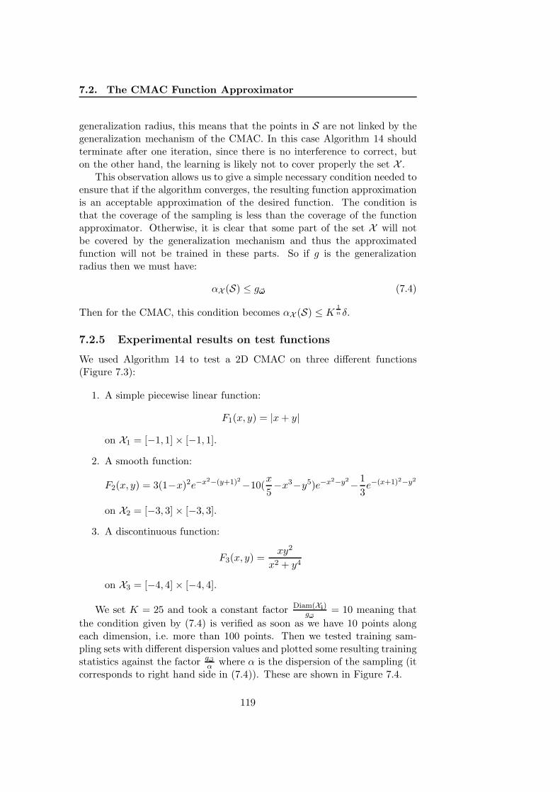
7.2. The CMAC Function Approximator
generalization radius, this means that the points in S are not linked by thegeneralization mechanism of the CMAC. In this case Algorithm 14 shouldterminate after one iteration, since there is no interference to correct, buton the other hand, the learning is likely not to cover properly the set X .
This observation allows us to give a simple necessary condition needed toensure that if the algorithm converges, the resulting function approximationis an acceptable approximation of the desired function. The condition isthat the coverage of the sampling is less than the coverage of the functionapproximator. Otherwise, it is clear that some part of the set X will notbe covered by the generalization mechanism and thus the approximatedfunction will not be trained in these parts. So if g is the generalizationradius then we must have:
αX (S) ≤ g~ω (7.4)
Then for the CMAC, this condition becomes αX (S) ≤ K1n δ.
7.2.5 Experimental results on test functions
We used Algorithm 14 to test a 2D CMAC on three different functions(Figure 7.3):
1. A simple piecewise linear function:
F1(x, y) = |x+ y|
on X1 = [−1, 1]× [−1, 1].
2. A smooth function:
F2(x, y) = 3(1−x)2e−x2−(y+1)2−10(x
5−x3−y5)e−x2−y2
−1
3e−(x+1)2−y2
on X2 = [−3, 3]× [−3, 3].
3. A discontinuous function:
F3(x, y) =xy2
x2 + y4
on X3 = [−4, 4]× [−4, 4].
We set K = 25 and took a constant factor Diam(Xi)g~ω
= 10 meaning that
the condition given by (7.4) is verified as soon as we have 10 points alongeach dimension, i.e. more than 100 points. Then we tested training sam-pling sets with different dispersion values and plotted some resulting trainingstatistics against the factor g~ω
α where α is the dispersion of the sampling (itcorresponds to right hand side in (7.4)). These are shown in Figure 7.4.
119

Chapter 7. Approximate Dynamic Programming
F1(x, y) F2(x, y) F3(x, y)
Figure 7.3: The three test functions
(a)
(b)
(c)
(d) F1F2F3m
emor
yti
me
(s.)
err.
2-n
orm
err.∞
-nor
m
g~ωα
g~ωα
Figure 7.4: Training of a 2D CMAC with three different functions usingsampling sets with decreasing dispersions. (a)-(b) errors in ∞-norm and2-norm. (c)-(d) computation time and memory used.
120

7.3. Reducing The State Space Exploration
The best results are obtained for the smooth function F2. For the othertwo, the results in infinity norm are due to values around the discontinuityfor F3 and in the corners for F1. Note that for F1, a much coarser value for g~ω
could have been used due to the linearity of the function. In the three cases,we see that after a certain dispersion value, the memory does not increaseany more. This means that a saturation threshold in interference has beenreached. From there, the convergence becomes more difficult (computationtime increases) while the global quality of the approximation (error in 2-norm) only slightly increases. This indicates that there is an optimal valuefor the factor g~ω
α in terms of quality against computational cost (for theCMAC used above, we can observe that this value is around 4, consideringthe three different test functions).
7.3 Reducing The State Space Exploration
To combat the curse of dimensionality, we then have two different mecha-nisms. Firstly the local generalization mechanism allows to update the valuefunction in a whole region of size g~ω from an update in one point. Secondly,it assumes that only a fraction of the state space is actually explored andthen only a small number of parameters needs actually to be updated (thisexplains the name “sparse coarse coding” used in [SB98]). In this section,we propose a heuristic to reduce the state space explored by dynamic pro-gramming algorithms presented so far.
Now we assume that we do not need to compute a control law on X butonly on particular subset X0 of it. Since the set X0 has no reason a priori tobe invariant, our idea is to try to build an invariant set which contains X0
and to apply approximate dynamic programming on it. It is well known thatthe smallest invariant that contains X0 is Reach(X0), the set reachable fromX0, thus it is clearly the ideal candidate. However, we saw in the secondpart of the thesis that computing reachable sets for systems with inputs wasa problem whose difficulty was comparable to that of optimal control prob-lems. So trying to compute Reach(X0) for all inputs is unrealistic. On theother hand, the closed-loop system using the optimistic controller becomesan autonomous system on which we can apply the algorithms developed inPart 2, so this is what we propose. Using the unbounded horizon algorithmdescribed in Section 3.6.2, we can get a sampling with a desired dispersion ofthe set reachable from X0 using the optimistic policy defined by a functionV i. We note it SReach(X0, V
i). If we use a CMAC to approximate the valuefunction, we saw that the dispersion of SReach(X0, V
i) had to be less thanthe generalization radius g~ω.
Then an iteration of our heuristic consists in two main steps:
1. The computation of a sampling Si = SReach(X0, Vi)
121

Chapter 7. Approximate Dynamic Programming
2. The iteration of a TD algorithm using all points of Si to get a newestimation V i+1 of the value function.
Then ideally, V i converges to the optimal value function and Si to asampling of the set reachable from X0 using the optimal feedback controller.Note that in practice, the TD algorithm can be iterated several times beforeupdating Si. Also to improve local exploration at each of these iterations,each point in Si can be added a random offset whose amplitude is less thanthe global dispersion of Si.
The major interest of this heuristic is that it allows to build automaticallythe domain on which we compute the value function. This can potentiallyavoid to compute it on large parts of the state space. The counter part of itis that as many optimizing heuristics, the algorithm may get stuck in a localoptimum. In fact, there is possibility that it converges to a value functionwhich is optimal on the invariant set that it induces but different from theoptimal value function on X .
The occurrence of such a situation is highly sensitive to the choice ofX0 and also to the initial estimation V 0 of the value function. It is thusimportant to use all the information available about the system and theproblem to do these choices. In particular if the value function is known atparticular points of the state space, these points should be included in X0
and V 0 initialized consequently.
7.4 Examples
7.4.1 Swing up of the Pendulum
We applied the heuristic of the previous section to the pendulum swing upproblem described in Section 6.5. Recall that the dynamics is defined by:
θ = −µθ + g sin θ + u. (7.5)
The state space is thus 2-dimensional, the two state variables being the angleθ and the angle velocity θ. the cost function is c(θ) = (1− cos(θ)).
In this example, there is a goal state, which is the vertical position withzero velocity, and an obvious set of initial states consisting in the possiblepositions of the pendulum. On the other hand, we do not know a prioriwhich velocity the pendulum will need to reach the goal position. Thus agood choice for X0 is the set defined by θ ∈ [−π, π] and θ = 0. Since theproblem is symmetric, we can even restrict to positive angles, then
X0 = (θ, θ) s.t.θ ∈ [0, π] and θ = 0
Note that the goal state, for which we know that the value function is 0, isactually in X0. On Figure 7.5 we show the set reachable from X0 using theinitial controller and then the reachable using the optimal controller.
122

7.4. Examples
(a) (b)θ
θ X0X0
Figure 7.5: (a) Reachable set using the initial controller. (b) Reachable setusing the optimal control law.
(a) (b)
Figure 7.6: (a) Value function computed on (θ, θ) ∈ [−π, π] × [−10, 10].(b)Value function computed on the set reachable from X0 = (θ ∈ [−π, π], θ =0).
We used a CMAC with a quantization vector δ = ( pi15 , 0.625) and a gen-
eralization radius g~ω = 6δ (corresponding to K = 36) and trained it withthe value 0 for θ = 0 and θ = 0. On Figure 7.6, we show a comparisonbetween the value function computed on the whole state space and its re-striction to the reachable set from X0. In the first case, the CMAC used1177 coefficients against 853 in the second case.
7.4.2 The Acrobot
The acrobot is a classic challenging under-actuated motor-control problem.It is basically a double pendulum where the torque is at the articulationbetween the “body” and “legs” (see Figure 7.7). The goal is to reach thevertical position for both the body and the legs and keep it with a zerovelocity.
123

Chapter 7. Approximate Dynamic Programming
g = 9.81, gravity accelerationm1 = 1, mass of acrobot bodym2 = 1, mass of acrobot legsl1 = .5, half-length of bodyl2 = .5, half-length of legsµ1 = .05, friction coefficient of bodyµ2 = .05, friction coefficient of legs−2 ≤ u ≤ 2, torque applied to legs.
θ1
θ2
Figure 7.7: The acrobot
The state variables are the angles θ1 and θ2 and the angle velocities θ1and θ2. The dynamics is given in a compact form by
(a11 a12
a21 a22
)(θ1θ2
)
=
(b1b2
)
(7.6)
where
a11 = (43m1 + 4m2)l21,
a22 = 43m2l
22,
a12 = a21 = 2m2l1l2cos(θ1 − θ2),
b1 = 2m2l2l1θ22 sin(θ2 − θ1) + (m1 + 2m2)l1g sin θ1 − µ1θ1 − u,
b2 = 2m2l1l2θ12
sin(θ1 − θ2) +m2l2g sin θ2 − µ2θ2 + u.
and the cost function used was
c(θ1, θ2) = 3− cos(θ1)− cos(θ2)−cos(θ1 − θ2)
2−
cos(θ1 + θ2)
2.
We used a CMAC with δ = (.125, .125, .48, 1) and K = 256. Figure 7.8shows a trajectory that we obtained projected in the plane (θ1, θ2). Fromthe bottom position with zero velocity, the controller manage to reach getnear the goal position (0, 0) but cannot stabilize.
7.5 Summary
In this chapter, we investigated the use of dynamic programming meth-ods to solve optimal control problems for a general class of systems. Morespecifically, we presented a framework for the design of temporal differencesalgorithms in continuous time and space. This framework is attractive asit clearly separates different issues related to the use of such algorithms,namely:
124

7.5. Summary
π
π
π2
π2
0
0
−π
−π−π2
−π2
θ1
θ2
Figure 7.8: A trajectory of the acrobot projected in the plane (θ1, θ2). Thestarting point is (−π, π).
125

Chapter 7. Approximate Dynamic Programming
1. the choice of the sampling trajectories and the controller used;
2. the representation of the optimal value function;
3. the update of the value function, based on the information providedby simulated trajectories.
After describing the context of continuous dynamic programming andour framework, we presented a continuous version of TD(λ) which is consis-tent after appropriate discretization with its original discrete version. Wethen discussed its efficiency with respect to the parameter λ, and presenteda variant, TD(∅), that we found to be experimentally as efficient as TD(λ)for the best values of λ. Then in the last chapter, we investigated the issue offunction approximation with local generalization and presented the CMAC,for which we tested the ability to represent various functions. Finally, inSection 7.3, we proposed to restrict the computation of the value functionto the set reachable from a subset of the state space, using a set of samplingtrajectories. This reachable set can be potentially much smaller than an ar-bitrarily chosen domain for the computation of the value function, in whichcase the method helps against the curse of dimensionality. Controlling thedispersion of these trajectories is then done to facilitate the convergence ofthe function approximation.
126

Part IV
Implementation andConclusion
127


Chapter 8
Implementation
8.1 Introduction
In this chapter, we describe Breach, a prototype toolbox that gathers all theimplementation we made of the various algorithms described in the thesis.This toolbox intends to provide a coherent set of routines for the analysisof deterministic models of dynamical systems. We tried to make it generic,efficient and flexible.Basically, genericity is achieved by the use of a robust numerical solver ofODEs; in the first part of the thesis, we showed how continuous systems,systems with inputs and a class of hybrid systems could be simulated bysolving ODEs. Efficiency relies on the implementation of the most compu-tationally demanding routines in C++. And flexibility is achieved by theuse of Matlab to implement easily high level routines, and to benefit from itsrich interface and plotting capabilities. In the following, we give an overviewof the toolbox organisation and features.
8.2 Organisation
The toolbox organisation relies on five distinct “modules”:
The Simulator is the essential module used to compute trajectories of thesystem;
The Sampling Module gathers some routines to manipulate samplingsets that are union of rectangular samplings, i.e. finite sets of pointsin hyper rectangles;
The CMAC Module is an efficient implementation of the CMAC func-tion approximator described in Section 7.2;
129

Chapter 8. Implementation
CMACLAB
Approx. DPReach Set
Simulation
Sampling
Figure 8.1: Modules interdependance diagram. An arrow means ’uses’. TheCMAC module is used for reach set computations, not as a function approx-imator but to store regions visited by trajectories.
The Reach set Module implements reachability algorithms described inPart 2, basic sampling reachability, and reachability using sensitivityanalysis, both for bounded and unbounded horizon;
The Approximate Dynamic Programming Module implements Tem-poral Differences algorithms described in Part 3.
The first three modules are independant and could be used for any otherpurpose, while reachability and TD routines heavily rely on the first three.Figure 8.1 provides a diagram showing the modules interdependance.
More details about each module are given in the following sections.
8.3 Simulation and Sensitivity Analysis using CVodes
Simulation is the first and maybe the most important step in the analysisof a dynamical system. The simulation module of the toolbox is based onCVodes solver, which implements efficient methods to solve both stiff andnon stiff ODEs, with the capacity to compute sensitivity functions. Anotherpositive feature of this solver is that it has a mature and highly tunable in-terface, with a complete documentation [HS06].
To solve an ODE of the form
x = f(t,x), x(0) = x0,
130

8.3. Simulation and Sensitivity Analysis using CVodes
CVodes needs at least that the user provides a routine computing the right-hand-side (rhs) function f . The core of the solver is implemented in the Clanguage but recently a Matlab interface was released that allows to writethe rhs function as a Matlab routine. However the repeated calls of theMatlab routine from the C solver dramatically decrease the performances ofthe solver. In our implementation we thus adopted a compromise betweenthe efficiency of C implementation and the flexibility of Matlab interface.We modified the existing Matlab interface of CVodes to accept rhs functionswritten in C.
Concretely, to set up the simulator of a system, the user has to writethree functions in C:
• An initialization function, InitFdata, to manage problem specificdata and parameters; it is used in particular to set up a CMAC usedas the value function to compute the control inputs;
• The RHS function f ;
• An update function,UpdateFdata, which is called by the solver dur-ing the computation of the trajectory after each successful step; thisfunction has primarily in charge
– the computation of input values;
– the mode changes of the system in case it is hybrid;
– the computation of sensitivity jumps in case of a transition.
Once these functions have been written and compiled using a dedicatedscript, the tuning of the solver (numerical method used, tolerances, sen-sitivity components to compute etc) can be done integrally from Matlabprompt or using Matlab scripts using the CVodes Matlab interface. Whenthe system is hybrid or has discontinuous inputs, transitions are handled us-ing Algorithm 1. Thus the user has to specify a value for hmax for the eventdetection and for hmin to limit the frequency of transitions (thus preventingzeno behaviors).
Once the simulator has been set up, trajectories of the system can becomputed by specifying their initial states and a time interval. Dependingon the routine called, we can obtain the trajectory values at specified timeinstants or points of the trajectory such that two consecutive points are notfurther than a certain value from each other. Additionnal informations suchas sensitivities or values of a value function along the trajectory can also becomputed.
131

Chapter 8. Implementation
8.4 Samplings
8.4.1 Definition of a Rectangular Sampling
To represent sampling sets, the toolbox uses rectangular samplings. Theseare basically sets of points which are at the center of hyper-rectangles. In itsmost basic form, a rectangular sampling is a structure S with the followingfields:
• dim is a vector indicating in which dimensions the rectangles have avolume; e.g if dim= 1, they are segments parallel to the x1 axis, and ifdim= (1, 3), they are flat rectangles parallel to the plane (x1, x3) andso on;
• pts is a list of points of dimension n
• epsi is the corresponding list giving the dimensions of the rectangles.
We call dispersion of the rectangular sampling the vector whose componentsare the maximal sizes of the rectangles in each dimension.
A sampling S can be used as a set of initial states for the computationof trajectories. When this is the case, the computed trajectories are storedin an additional field traj, and another additional field Xf store their endpoints. If the expansion function is required, the appropriate sensitivitiesare computed and the dimensions epsi of the rectangles are used for the ǫused in Chapter 4.
8.4.2 Refinement
A generic routine Refine allows to refine a rectangular sampling S. Eachrectangle in S is sampled using Sukharev grids as described in Section 3.3,except that cubes are replaced by hyper-rectangles. Local refinement is ob-tained by preselecting the points and their rectangles that we want to refine.The new sampling can be obtained as a new independant rectangular sam-pling or if we want hierarchical refinement as an additional field child ofS.
8.4.3 Plotting
Several routines allow the visualization of sampling sets and sampling tra-jectories.
• SplotPts and SplotXf allows to plot points, and trajectory end pointsof S;
• SplotTraj plot trajectories of S in the state space;
132
8.5. The CMAC Module
• SVoxelPts vizualise the rectangles of the sampling
• SVoxelTraj and SVoxelXf vizualize the expansion function aroundthe trajectories and their end points.
Optionnally if the dimension of the state space is more than 2 or 3, aprojection vector can be specified.
8.5 The CMAC Module
The CMAC module implements the creation and the usage of CMAC ob-jects. Each of them is an individual function approximator and its principalcharacteristics are
• its number of dimensions n,
• its quantization vector δ,
• and its generalization factor K
which are explained in Section 7.2. Additionally, the CMAC can be madeperiodic in specified dimensions.
A CMAC is equipped with a hash table that serves for the storage of itsparameters. Each entry of this table corresponds to one δ-region in the statespace, as described in Section 3.5.2. It stores the K corresponding weightswhen used as a function approximator or it is just marked as “visited” whenused within a reachability routine.
The basic operations that can be performed on CMAC objects are
• the creation of new object by specifying the above characteristics
• the training at one point or at a set of points as described in 7.2
• the output of the interpolated functions or of one of its partial deriva-tives;
Additional routines allows to plot the function approximated by a CMACin 1D or as a surface w.r.t. 2 state variables.
An important feature of this module is the fact that we can create,modify, test and save easily different instances of CMAC objects. This addsa great deal of flexibility in their use.
133

Chapter 8. Implementation
8.6 Reachability and Safety Verification
The toolbox implements the sampling-based reachability algorithms de-scribed in Chapter 3 and Chapter 4. The implemented routines are de-noted by xxreach where xx can be b, for “box”, s for “sensitivity”, sb forboth “box” and “sensitivity”, or vb for “very basic”. They require threearguments:
• an initial sampling S0;
• a desired dispersion vector δ;
• and either
– a time interval [t0, t1], on which to perform bounded horizonreachability;
– or a time step T , in which case unbounded horizon reachability isperformed using Algorithm 4 described at the end of Chapter 3.
They return a sampling with the set of computed trajectories.
The four routines differ mainly on the refinement strategy and the stop-ping criterion used:
• vbreach never refines the initial sampling. It only computes the tra-jectories starting from the points in S0. It can be useful to make aquick-and-dirty unbounded horizon analysis;
• breach refines locally the initial sampling when new regions are visited(Algorithm 2 of Chapter 3);
• sreach refines locally the initial sampling based on the computationof the expansion function using sensitivity (Algorithm 6 of Chapter 4);
• sbreach mixes the use of boxes and expansion; it stops either whenexpansion is less that δ or when no new region is visited. This way, theexpansion criterion can avoid unnecessary refinements even when newregions were discovered. Conversely, if the expansion is highly over-approximated (or if it diverges due to a grazing phenomenon in thehybrid case), the eventual absence of new boxes forces the algorithmto terminate.
The verification Algorithm 8 is implemented by the routine verif. Itrequires the same inputs as the reachability routines, plus the specificationsof the bad set. Those take the form of a simple user-provided function whoseinput is a trajectory and its corresponding expansion function and outputis bad, safe or uncertain.
134

8.7. Temporal Differences Algorithms
8.7 Temporal Differences Algorithms
The main routine of the Approximate Dynamic Programming module isnamed td. It takes a CMAC object and a structure with different optionsand returns an updated CMAC object and a structure with statistics on therun. It implements the generic Temporal Differences algorithm described inChapter 6. The main possible options are
• A sampling S;
• The time interval [0, T ];
• The λ parameter;
• A number of iterations nb_iter.
It performs nb_iter iterations during which for each points xi in S,
• it picks randomly a points x in the rectangle associated to xi;
• it computes the trajectory ξx on [O,T ];
• it computes a TD(λ) estimation of the value function;
• it uses this estimation to train the CMAC at points visited by thetrajectory.
Statistics returned by the routine mainly include the average performanceof the computed trajectories and the average Hamiltonian error. The per-formance is more relevant when monitoring the actual progress of a coarsesuboptimal controller while the Hamiltonian error is rather used when try-ing to get a precise approximation of the optimal value function.
It is important to recall that the controller used for the computation oftrajectories is problem specific. In Section 5.3, it is suggested to use the op-timistic controller obtained by solving the optimization problem (5.13). Thissolution can be obtained and implemented within the C function UpdateFdata,from where the CMAC object can be called to get values of the current valuefunction approximation and its derivatives. But different controllers can beused as well when we have good reasons to do so. In particular at the be-ginning of the process, when the value function has just been initialized, itis often much better to use a controller with initially guessed values or thatfirst tries to stabilize the system.
135

Chapter 8. Implementation
136

Chapter 9
Conclusion and Perspectives
In this thesis, we presented the theory and implementation of a coherent setof methods devoted to the analysis of a large class of dynamical systems.Three topics were addressed:
• simulation;
• reachability analysis and safety verification;
• controller synthesis via approximate dynamic programming techniques.
9.1 Contributions
We believe that the main contributions of the thesis are the followings.Firstly we developed a novel and general trajectory-based method for thereachability analysis of continuous and piecewise continuous systems. Theonly requirement is that the system can be accurately simulated using a stan-dard numerical solver, which means that the applicability and the scalabilityof the method is large. We showed that we could obtain conservative over-approximation of reachable sets using finite number of trajectories and thuscould verify formally safety properties. We think that this opens new per-spectives for the formal analysis of complex systems that were not possiblebefore. This methodology is also more likely to be accepted by practitionerswho already use simulation as a key validation tool.
The second main contribution is the development of a flexible frame-work for the application of approximate dynamic programming techniques,in particular temporal difference algorithms adapted to systems in contin-uous time and space. We showed how to efficiently generate samplingsof trajectories taking in consideration the generalization properties of thefunction approximators used in these techniques. We also detailed how touse sampling-based reachability techniques to restrict the exploration of thestate space and thus limit the computational cost of the method.
137

Chapter 9. Conclusion and Perspectives
9.2 Perspectives
This work can be extended in number of ways. Firstly we can extend therange of mathematical models that we consider, e.g. to differential alge-braic equation models often arising naturally in the field of analog circuits[DDM04], and for which sensitivity analysis is also already well-studied[BL02, SGB99]. Also from a technical point of view, we can adapt ourimplementation to the use specialized simulation tools widely used in theindustry like the circuit simulator SPICE.
The verification part of the thesis is also closely related to the method-ology presented in [GP06], the main difference being that in this work theconcept of bisimulation is used to characterize the relative coverage of tra-jectories. Thus in the spirit of the extensions that were made in this othercontext in [FGP06, FP06], we believe that we can extend our technique tothe verification of temporal logic properties.
Aside from those considerations, a number of practical and theoreticalissues related to approximate dynamic programming can still be explored.In that matter, the flexibility of our framework and implementation allowsa great deal of possible experimentations of new algorithms and techniques.
138

Bibliography
[ABDM00] E. Asarin, O. Bournez, T. Dang, and O. Maler. Approx-imate reachability analysis of piecewise-linear dynamicalsystems. In B. Krogh and N. Lynch, editors, Hybrid Sys-tems: Computation and Control, LNCS 1790, pages 20–31.Springer-Verlag, 2000.
[AC84] J.P. Aubin and A. Cellina. Differential Inclusions: Set-valued Maps and Viability Theory. Springer, 1984.
[ACH+95] R. Alur, C. Courcoubetis, N. Halbwachs, T.A. Henzinger,P.-H. Ho, X. Nicollin, A. Olivero, J. Sifakis, and S. Yovine.The algorithmic analysis of hybrid systems. TheoreticalComputer Science, 138:3–34, 1995.
[ADG03] E. Asarin, T. Dang, and A. Girard. Reachability anal-ysis of nonlinear systems using conservative approxima-tion. In Oded Maler and Amir Pnueli, editors, HybridSystems: Computation and Control, LNCS 2623, pages20–35. Springer-Verlag, 2003.
[ADG05] E. Asarin, T. Dang, and A. Girard. Hybridization meth-ods for verification of non-linear systems. In ECC-CDC’05joint conference: Conference on Decision and ControlCDC and European Control Conference ECC, 2005.
[ADM01a] E. Asarin, T. Dang, and O. Maler. d/dt: a tool for reach-ability analysis of continuous and hybrid systems. In Non-linear Control Systems NOLCOS, Invited session, St Pe-tersburg, 2001.
[ADM01b] E. Asarin, T. Dang, and O. Maler. d/dt: A verificationtool for hybrid systems. In Hybrid Systems: Computationand ControlConference on Decision and Control, Invitedsession “New Developments in Verification Tools for Hy-brid Systems, 2001.
139

Bibliography
[ADM02] E. Asarin, T. Dang, and O. Maler. The d/dt tool for verifi-cation of hybrid systems. In Computer Aided Verification,LNCS 2404, pages 365–370. Springer-Verlag, 2002.
[AGM06] Colas Le Guernic Antoine Girard and Oded Maler. Effi-cient computation of reachable sets of linear time-invariantsystems with inputs. In Hybrid Systems : Computa-tion and Control, volume 3927 of LNCS, pages 257–271.Springer-Verlag, 2006.
[Alb75] J.S. Albus. A new approach to manipulator control : Thecerebellar model articulation controller (cmac). Transac-tions ASME, September 1975.
[AMP95] E. Asarin, O. Maler, and A. Pnueli. Reachability analy-sis of dynamical systems having piecewise-constant deriva-tives. Theoretical Computer Science, 138:35–66, 1995.
[An91] P.-C. E. An. An improved multi-dimensional CMAC neu-ral network: receptive field function and placement. PhDthesis, University of New Hampshire, 1991.
[AP04] Rajeev Alur and George J. Pappas, editors. Incremen-tal Search Methods for Reachability Analysis of Continu-ous and Hybrid Systems., volume 2993 of LNCS. Springer,2004.
[Bar06] R. Barrio. Sensitivity analysis of odes/daes using the tay-lor series method. SIAM Journal on Scientific Computing,27(6):1929–1947, 2006.
[Bat06] G. Batt. Validation de modeles qualitatifs de reseaux deregulation genique : une methode basee sur des techniquesde verication formelle. PhD thesis, Universite JosephFourier (Grenoble-I), February 2006.
[BCLM05] M. S. Branicky, M. M. Curtiss, J. Levine, and S. Mor-gan. Sampling-based reachability algorithms for controland verification of complex systems. In Proc. ThirteenthYale Workshop on Adaptive and Learning Systems, June2005.
[BCP89] K. E. Brenan, S. L. Campell, and L. R. Petzold. Nu-merical Solution of Initial Value Problems in OrdinaryDifferential-Algebraic Equations. North Holland Publish-ing Co., 1989.
140

Bibliography
[Bel57] R. Bellman. Dynamic Programming. Princeton UniversityPress, Princeton, New Jersey, 1957.
[Ber01a] D. P. Bertsekas. Dynamic Programming and Optimal Con-trol, Vol. I, 2nd Ed. Athena Scientific, Belmont, MA, 2001.
[Ber01b] D. P. Bertsekas. Dynamic Programming and Optimal Con-trol, Vol. II, 2nd Ed. Athena Scientific, Belmont, MA,2001.
[BF06] A. Bhatia and E. Frazzoli. Resolution-complete safety fal-sification of continuous time systems. In IEEE Conf. onDecision and Control, 2006.
[BL01] Vishal Bahl and Andreas A. Linninger. Modeling ofcontinuous-discrete processes. In HSCC, pages 387–402,2001.
[BL02] Paul I. Barton and Cha Kun Lee. Modeling, simulation,sensitivity analysis, and optimization of hybrid systems.ACM Trans. Model. Comput. Simul., 12(4):256–289, 2002.
[BSD+01a] C. Belta, J. Schug, T. Dang, V. Kumar, G.J. Pappas,H. Rubin, and P. Dunlap. Stability and reachability anal-ysis of a hybrid model of luminescence in the marine bac-terium vibrio fisheri. In Proceedings of CDC, 2001.
[BSD+01b] C. Belta, J. Schug, T. Dang, V. Kumar, G.J. Pappas,H. Rubin, and P. Dunlap. Stability and reachability anal-ysis of a hybrid model of luminescence in the marine bac-terium vibrio fisheri. In Proceedings of CDC, 2001.
[BT00] A. Bemporad and F.D. Torrisi. Inner and outter approxi-mation of polytopes using hyper-rectangles. Technical re-port, Automatic Control Lab, ETH, Zurich, 2000.
[BTM00] A. Bemporad, F.D. Torrisi, and M. Morari. Optimization-based verification and stability characterization of piece-wise affine and hybrid systems. In B. Krogh and N. Lynch,editors, Hybrid Systems: Computation and Control, LNCS1790, pages 45–58. Springer-Verlag, 2000.
[CK98] A. Chutinan and B.H. Krogh. Computing polyhedral ap-proximations to dynamic flow pipes. In Proc. of the 37thAnnual International Conference on Decision and Control,CDC’98. IEEE, 1998.
141

Bibliography
[Cou02] R. Coulom. Reinforcement Learning Using Neural Net-works, with Applications to Motor Control. PhD thesis,Institut National Polytechnique de Grenoble, 2002.
[Dan00] T. Dang. Verification et Synthese des Systemes Hybrides.PhD thesis, Institut National Polytechnique de Grenoble,October 2000.
[Dan05] Thao Dang. Reachability-based technique for idle speedcontrol synthesis. International Journal of Software Engi-neering and Knowledge Engineering IJSEKE, 15 (2), 2005.
[DDM04] T. Dang, A. Donze, and O. Maler. Verification of ana-log and mixed-signal circuits using hybrid systems tech-niques. In Alan J. Hu and Andrew K. Martin, editors,FMCAD’04 - Formal Methods for Computer Aided De-sign, LNCS 3312, pages 21–36. Springer-Verlag, 2004.
[DH06] V. Donde and I.A. Hiskens. Shooting methods for locat-ing grazing phenomena in hybrid systems. InternationalJournal of Bifurcation and Chaos, 16(3):671–692, March2006. 2006.
[DM98] T. Dang and O. Maler. Reachability analysis via face lift-ing. In T.A. Henzinger and S. Sastry, editors, Hybrid Sys-tems: Computation and Control, LNCS 1386, pages 96–109. Springer-Verlag, 1998.
[DN07] Thao Dang and Tarik Nahhal. Randomized simulation ofhybrid systems. Technical Report TR-2006-11, Verimag,Centre Equation, 38610 Gieres, January 2007.
[Doy96] Kenji Doya. Temporal difference learning in continuoustime and space. In David S. Touretzky, Michael C. Mozer,and Michael E. Hasselmo, editors, Advances in Neural In-formation Processing Systems, volume 8, pages 1073–1079.The MIT Press, 1996.
[Doy00] Kenji Doya. Reinforcement learning in continuous timeand space. Neural Computation, 12(1):219–245, 2000.
[EKP01] Joel M. Esposito, Vijay Kumar, and George J. Pappas.Accurate event detection for simulating hybrid systems.In HSCC, pages 204–217, 2001.
[FG94] U. Feldmann and M. Gunther. The DAE-index in electriccircuit simulation. In I. Troch and F. Breitenecker, editors,
142

Bibliography
Proc. IMACS, Symposium on Mathematical Modelling, 4,pages 695–702, 1994.
[FGP06] Georgios E. Fainekos, Antoine Girard, and George J. Pap-pas. Temporal logic verification using simulation. In FOR-MATS, pages 171–186, 2006.
[Fil88] A.F. Filippov. Differential Equations with DiscontinuousRighthand Sides. Kluwer, 1988.
[FKRM06] Goran Frehse, Bruce H. Krogh, Rob A. Rutenbar, andOded Maler. Time domain verification of oscillator circuitproperties. Electr. Notes Theor. Comput. Sci., 153(3):9–22, 2006.
[Flo97] Henrik Floberg. Symbolic Analysis in Analog IntegratedCircuit Design. Kluwer Academic Publishers, Boston,1997.
[FP06] Georgios E. Fainekos and George J. Pappas. Robustness oftemporal logic specifications. In FATES/RV, pages 178–192, 2006.
[GF06] Rob A. Rutenbar Goran Frehse, Bruce H. Krogh. Verifyinganalog oscillator circuits using forward/backward abstrac-tion refinement. In DATE 2006: Design, Automation andTest in Europe, March 2006.
[Gir05] A. Girard. Reachability of uncertain linear systems usingzonotopes. In Hybrid Systems : Computation and Control,LNCS 3414, pages 291–305. Springer, 2005.
[Gir06] A. Girard. Analyse algorithmique des systemes hybrides.PhD thesis, Universite Joseph Fourier (Grenoble-I), Febru-ary 2006.
[GM98] M.R. Greenstreet and I. Mitchell. Integrating projections.In T.A. Henzinger and S. Sastry, editors, Hybrid Systems:Computation and Control, LNCS 1386, pages 159–1740.Springer-Verlag, 1998.
[GM99a] M.R. Greenstreet and I. Mitchell. Reachability analy-sis using polygonal projections. In F. Vaandrager andJ. van Schuppen, editors, Hybrid Systems: Computationand Control, LNCS 1569, pages 76–90. Springer-Verlag,1999.
143

Bibliography
[GM99b] M.R. Greenstreet and I. Mitchell. Reachability analy-sis using polygonal projections. In F. Vaandrager andJ. van Schuppen, editors, Hybrid Systems: Computationand Control, LNCS 1569, pages 76–90. Springer-Verlag,1999.
[GNRR93] R.L. Grossman, A. Nerode, A.P. Ravn, and H. Rischel,editors. Hybrid Systems, LNCS 736. Springer-Verlag, 1993.
[GP06] Antoine Girard and George J. Pappas. Verification us-ing simulation. In Hybrid Systems : Computation andControl, volume 3927 of LNCS, pages 272–286. Springer-Verlag, 2006.
[Gre96] M.R. Greenstreet. Verifying safety properties of differen-tial equations. In R. Alur and T.A. Henzinger, editors,Computer Aided Verification, CAV’96, LNCS 1102, pages277–287. Springer-Verlag, 1996.
[GT01] J. Gouze and S. Tewfik. A class of piecewise linear dif-ferential equations arising in biological models. Technicalreport, INRIA, 2001.
[Hai01] Ernst Hairer. Geometric integration of ordinary differen-tial equations on manifolds. Journal BIT Numerical Math-ematics, 41, 2001.
[HH91] Gunther Hammerlin and Karl-Heinz Hoffmann. NumericalMathematics. Springer-Verlag, 1991.
[HHB02] W. Hartong, L. Hedrich, and E. Barke. On discrete mod-elling and model checking for nonlinear analog systems. InComputer Aided Verification. Springer, 2002.
[His05] I.A. Hiskens. Non-uniqueness in reverse time of hybridsystem trajectories. In Hybrid Systems : Computation andControl, volume 3414 of LNCS, pages 257–271. Springer-Verlag, 2005.
[HLW96] Ernst Hairer, Christian Lubich, and Gerhard Wanner. Ge-ometric Numerical Integration. Structure-Preserving Al-gorithms for Ordinary Differential Equations., volume 14of Springer Series in Comput. Mathematics,. Springer-Verlag, second edition, 1996.
[HLW03] Ernst Hairer, Christian Lubich, and Gerhard Wanner. Ge-ometric Numerical Integration. Structure-Preserving Algo-
144

Bibliography
rithms for Ordinary Differential Equations., volume 31 ofSeries in Comput. Mathematics. Springer, 2003.
[HNW93] Ernst Hairer, Syvert Paul Norsett, and Gerhard Wanner.Solving Ordinary Differential Equations I. Nonstiff Prob-lems., volume 8 of Springer Series in Comput. Mathemat-ics,. Springer-Verlag, second edition, 1993.
[HP00] I.A. Hiskens and M.A. Pai. Trajectory sensitivity anal-ysis of hybrid systems. IEEE Transactions on Circuitsand Systems I: Fundamental Theory and Applications,47(2):204–220, February 2000.
[HPNBL+05] A. C. Hindmarsh, K. E. Grant P. N. Brown, S. L. Lee,D. E. Shumaker R. Serban, and C. S. Woodward. Sun-dials: Suite of nonlinear and differential/algebraic equa-tion solvers. ACM Transactions on Mathematical Soft-ware, 31(3):363–396, 2005.
[HS74] M.W. Hirsch and S. Smale. Differential Equations, Dy-namical Systems and Linear Algebra. Academic Press,1974.
[HS98] Gabor Horvath and Tamas Szabo. Higher order cmacand its efficient hardware realization. In NC, pages 72–78, 1998.
[HS06] A. C. Hindmarsh and R. Serban. User Documentation forcvodes v2.4.0, March 2006.
[HW96] Ernst Hairer, , and Gerhard Wanner. Solving OrdinaryDifferential Equations II. Stiff and Differential-AlgebraicProblems., volume 14 of Springer Series in Comput. Math-ematics,. Springer-Verlag, second edition, 1996.
[IBWG90] W. Thomas Miller III, Brian A. Box, Erich C. Whitney,and James M. Glynn. Design and implementation of ahigh speed cmac neural network. In NIPS, pages 1022–1027, 1990.
[KA99] Aleksander Kolcz and Nigel M. Allinson. Basis functionmodels of the cmac network. Neural Netw., 12(1):107–126,1999.
[Kap04] Jim Kapinski. Verification and Synthesis of Hybrid Sys-tems Using Proximity-Based Automata. PhD thesis,Carnegie Mellon University, August 2004.
145

Bibliography
[KKMS03] Jim Kapinski, Bruce H. Krogh, Oded Maler, and OlafStursberg. On systematic simulation of open continuoussystems. In HSCC, pages 283–297, 2003.
[Kor05] A. Korotayev. A compact macromodel of world systemevolution. Journal of World-Systems Research, 11(1):79–83, July 2005.
[KW97] L. Kocis and W. J. Whiten. Computational investigationsof low-discrepancy sequences. ACM Trans. Math. Softw.,23(2):266–294, 1997.
[LaV06] S. M. LaValle. Planning Algorithms. Cambridge Uni-versity Press, Cambridge, U.K., 2006. Available athttp://planning.cs.uiuc.edu/.
[LBL04] Steven M. LaValle, Michael S. Branicky, and Stephen R.Lindemann. On the relationship between classical gridsearch and probabilistic roadmaps. I. J. Robotic Res.,23(7-8):673–692, 2004.
[LYL04] S. R. Lindemann, A. Yershova, and S. M. LaValle. Incre-mental grid sampling strategies in robotics. In ProceedingsWorkshop on Algorithmic Foundations of Robotics, pages297–312, 2004.
[MAGC91] W. T. Miller, E. An, F. H. Glanz, and M. J. Carter. Thedesign of cmac neural networks for control. In O. Sim-ula, editor, Proceedings of the International Conferenceon Artificial Neural Networks ICANN’91. Elsevier SciencePublishers B.V., 1991.
[Mit02] I. Mitchell. Application of level set methods to control andreachability problems in continuous and hybrid systems.PhD thesis, Stanford University, August 2002.
[MM99] R. Munos and A. Moore. Variable resolution discretizationfor high-accuracy solutions of optimal control problems. InInternational Joint Conference on Artificial Intelligence,1999.
[Mun00] Remi Munos. A study of reinforcement learning in the con-tinuous case by the means of viscosity solutions. MachineLearning, 40(3):265–299, 2000.
[PB96] Taeshin Park and Paul I. Barton. State event location indifferential-algebraic models. ACM Trans. Model. Com-put. Simul., 6(2):137–165, 1996.
146

Bibliography
[Ran06] A. Rantzer. Relaxed dynamic programming in switchingsystems. IEE Proceedings - Control Theory and Applica-tions, 153(5):567 – 574, September 2006.
[SB98] R. S. Sutton and A. G. Barto. Reinforcement Learning:An Introduction. MIT Press, Cambridge, MA, 1998.
[SB06] A. B. Singer and P. I. Barton. Bounding the solutions ofparameter dependent nonlinear ordinary differential equa-tions. SIAM Journal on Scientific Computing, 27(6):2167–2182, 2006.
[Set96] J.A. Sethian. Level Set Methods : Evolving Interfaces inGeometry, Fluid Mechanics, Computer Vision, and Mate-rials Science. Cambridge, 1996.
[SGB91] L. F. Shampine, I. Gladwell, and R. W. Brankin. Reliablesolution of special event location problems for odes. ACMTrans. Math. Softw., 17(1):11–25, 1991.
[SGB99] William F. Feehery Santos Galan and Paul I. Bar-ton. Parametric sensitivity functions for hybrid dis-crete/continuous systems. Applied Numerical Mathemat-ics, 31(1):17–47, September 1999.
[SH05] R. Serban and A. C. Hindmarsh. Cvodes: the sensitivity-enabled ode solver in sundials. In Proceedings ofIDETC/CIE 2005, Long Beach, CA., Sept. 2005.
[Son98] E.D. Sontag. Mathematical Control Theory. DeterministicFinite-Dimensional Systems, volume 6 of Texts in AppliedMathematics. Springer-Verlag, New York, second edition,1998.
[Sut88] Richard S. Sutton. Learning to predict by the methods oftemporal differences. Machine Learning, 3:9–44, 1988.
[Sut96] R. S. Sutton. Generalization in reinforcement learning:Successful examples using sparse coarse coding. In Ad-vances in Neural Information Processing Systems 8, pages1038–1044. MIT Press, 1996.
[Tes95] Gerald Tesauro. Temporal difference learning and TD-Gammon. Communications of the ACM, 38(3):58–68,March 1995.
[TR96] John N. Tsitsiklis and Benjamin Van Roy. An analysis oftemporal-difference learning with function approximation.Technical Report LIDS-P-2322, 1996.
147

Bibliography
[TR05] Saurabh K. Tiwary and Rob A. Rutenbar. Scalable trajec-tory methods for on-demand analog macromodel extrac-tion. In DAC, pages 403–408, 2005.
[Tsi02] John N. Tsitsiklis. On the convergence of optimistic policyiteration. Journal of Machine Learning Research, 3:59–72,2002.
[TTR06] Saurabh K. Tiwary, Pragati K. Tiwary, and Rob A. Ruten-bar. Generation of yield-aware pareto surfaces for hierar-chical circuit design space exploration. In DAC, pages31–36, 2006.
[TVR97] John N. Tsitsiklis and Benjamin Van Roy. An analysis oftemporal-difference learning with function approximation.IEEE Transactions on Automatic Control, 42(5):674–690,May 1997.
[TWMGLGK87] III Thomas W. Miller, Filson H. Glanz, and III L. Gor-don Kraft. Application of a general learning algorithmto the control of robotic manipulators. Int. J. Rob. Res.,6(2):84–98, 1987.
[vdSS00] A.J. van der Schaft and H. Schumacher. An Introduction toHybrid Dynamical Systems, volume 251 of Lecture Notes inControl and Information Sciences. Springer-Verlag, Lon-don, 2000.
[Wic00] T. Wichmann. Computer aided generation of approximateDAE systems for symbolic analog circuit design. In Proc.Annual Meeting GAMM, 2000.
[WPHH99] T. Wichmann, R. Popp, W. Hartong, and L. Hedrich. Onthe simplification of nonlinear DAE systems in analog cir-cuit design. In Computer Algebra in Scientific Computing.Springer, 1999.
148