scale-up of mechanically agitated flotation processes based on the
TRANSCRIPT
SCALE-UP OF MECHANICALLY AGITATED
FLOTATION PROCESSES
BASED ON
THE PRINCIPLES OF DIMENSIONAL
SIMILITUDE
By
Marius Truter
Thesis submitted in partial fulfilment of the requirements for the Degree
of
MASTER OF SCIENCE IN ENGINEERING
(MINERAL PROCESSING)
in the Department of Process Engineering
at the University of Stellenbosch
Supervised by
Prof C Aldrich
Stellenbosch
December 2010
i
Declaration
I, the undersigned, hereby declare that the work contained in this thesis is my own
original work and that I have not previously in its entirety or in part submitted it at any
university for a degree.
10 September 2010
Signature Date
Copyright © 2010 Stellenbosch University
All rights reserved
ii
Abstract
The use of dimensional analysis to scale-up mechanically agitated flotation processes
and to identify deficiencies in froth flotation plants was explored. The full range of
operating variables was considered, such as particle size distribution, reagent suite,
conditioning time, retention time, machine geometry, aeration, solids suspension, power
requirements and turbulence. Dimensional analysis offers a methodology to combine
variables into dimensionless groups to guide the scale-up process based on the notion of
similarity. Ten dimensionless groups were developed and combined with metallurgical
variables, such as liberation, reagents dosage and flow diagrams to produce a scale-up
and evaluation tool, applicable to any mechanically agitated flotation process. In many
hydrodynamic studies, the researchers considered hydrodynamic variables based on
rotor diameter. In this case the hydrodynamic variables based on rotor diameter
represent mechanism “ability”, while parameters based on cell diameter are considered
“requirement”.
Dimensionless groups have also been applied to the definition of basic parameters of the
kinetic constant, such as floatability, bubble surface area flux and froth recovery factor.
It also showed that the bubble surface area flux has a maximum with increased aeration,
where similar models do not show this dependence.
Analysis by computational fluid dynamics and Perspex modelling revealed valuable
insight into the inner working of the Wemco flotation machine, such as air dispersion,
turbulence levels, separation zones and solids concentration. Design changes to the
rotor, disperser, hood and geometrical lay-out produced a marked improvement in
flotation conditions. It also supported certain dimensionless numbers measured in full
scale plants.
Case studies confirmed that almost all flotation plants, irrespective of the minerals
floated, suffer from the same deficiencies. Dimensional similitude offers a unique tool to
identify these deficiencies and to predict the effect of recommended improvements. In
almost every case where the fundamental requirement of similarity was applied, an
improvement in performance was observed. Finally a new algorithm is proposed for the
scale-up of flotation plants and the application is demonstrated in the design and testing
of a pilot plant.
iii
Opsomming
Die gebruik van dimensionele analise in die opskaal van flottasieprosesse en die
identifisering van flottasieaanlegprobleme is ondersoek. Die volle bereik van
bedryfsveranderlikes is ondersoek, soos partikelgrootte, kondisioneringstyd, retensietyd,
geometrie, lugvloei, suspensie van vastestowe, turbulensie en drywingsvereistes.
Dimensielose analise is die proses waardeur veranderlikes deur wiskundige manipulasie
gekombineer word in dimensielose groepe. Tien dimensielose groepe is ontwikkel en is
tesame met metallurgiese veranderlikes soos vrystelling, reagensdosering en vloei-
diagramme gekombineer om gebruik te word om gelykvormigheid te bewerkstellig.
Hierdie proses is van toepassing op enige flottasieproses gebaseer op meganies
geagiteerde toerusting.
Dimensielose groepe is ook gebruik in die definisie en kwantifisering van turbulensie,
agitasie, geometrie, suspensie van vastestowe, verspreiding van lug en drywings-
vereistes. Daarbenewens is die groepe gebruik in die definisie van die basiese
veranderlikes van die kinetiese konstante soos lugborreloppervlakvloed, suspensie, en
herwinning in die skuimfase. Die groepe is ook gebruik in die bewys dat die
lugborreloppervlakvloed ´n maksimum het met toename in lugvloei. In baie gevalle word
hidrodinamiese veranderlikes uitgedruk in terme van die rotordiameter en in hierdie
studie word dit beskou as meganisme “vermoë”. Die hidrodinamiese veranderlikes
gebaseer op sel-diameter word beskou as “behoefte”.
Berekeningsvloeidinamika en Perspex modellering het waardevolle insig verskaf in die
binne-werking van die Wemco flottasiemasjien soos lugverspreiding, turbulensie en
partikelkonsentrasie en is ook gebruik om sekere dimensielose getalle wat in volskaalse
aanlegte gemeet is, te verifieer. Gevallestudies het bevestig dat feitlik alle
flottasieaanlegte, ongeag die soort mineraal, gebuk gaan onder dieselfde afwykings.
Dimensionele analise bied ‘n eenvoudige benadering om hierdie afwykings te identifiseer
en om die effek van veranderings te voorspel. In alle gevalle waar die beginsels van
gelykvormigheid slaafs gevolg is, het n merkbare verbetering in prestasie voorgekom.
Ten slotte is ´n nuwe opskaleringsalgoritme ontwikkel en is die toepassing daarvan
gedemonstreer deur die ontwerp en toets van ´n loodsaanleg, gebaseer op die Wemco
geometrie.
iv
TABLE OF CONTENTS.
CHAPTER 1: INTRODUCTION. ........................................................................ 1
CHAPTER 2: A LITERATURE REVIEW ON DIMENSIONAL ANALYSIS AND SCALE-UP OF FLOTATION. .................................................................................. 7
2.1. Dimensional analysis and dimensionless numbers. ..................................... 7
2.2. Dimensions and units. ................................................................................. 8
2.3. Dimensional homogeneity. .......................................................................... 8
2.4. Typical results from a dimensional analysis... ............................................. 8
2.5. Methods of performing dimensional analysis. ............................................. 9
2.6. Choice of variables. ................................................................................... 13
2.7. Wrong choice of physical properties. ......................................................... 14
2.8. Similitude. ................................................................................................. 14
2.9. Dimensional analysis and flotation. ........................................................... 14
2.10. Flotation performance and dimensionless numbers. ............................... 18
2.11. Summary. ................................................................................................ 19
CHAPTER 3: DIMENSIONAL ANALYSIS OF A FLOTATION PROCESS. .................. 21
3.1. Dimensional analysis. ................................................................................ 21
3.2. Relevance list and linear independence. .................................................... 22
3.3. Buckingham -Theorem based on repeating variables. ............................. 22
3.4. Combination of some groups. .................................................................... 25
3.5. Dimensionless numbers and transformation equations. ............................ 25
3.6. Dimensionless kinetic constant. ................................................................ 27
3.7. Characterization of plant deficiencies based on a schedule of dimensionless numbers. .......................................................................................................... 39
3.8. Partial similarity. ....................................................................................... 46
3.9. Practical plant measurements. .................................................................. 47
v
3.10. Deficiencies in industrial plants based on the schedule of dimensionless parameters ....................................................................................................... 59
3.11. Dimensionless comparison of industrial designs. .................................... 61
3.12. Summary for the application of the schedule of dimensionless numbers. 61
CHAPTER 4: INTERPRATIVE RESULTS OF A CFD ANALYSIS OF FLOTATION CELL HYDRODYNAMICS. ........................................................................................... 64
4.1. Design data. .............................................................................................. 64
4.2. CFD model. ................................................................................................ 67
4.3. CFD RESULTS. ............................................................................................ 68
4.4. Mathematical procedure to calculate the mineral recovery rate potential. 75
4.5. Interpolation of Recovery rate potential data supplied by client. .............. 77
4.6. Bubble particle collision frequency. ........................................................... 81
4.7. Streamline plots. ....................................................................................... 82
4.8. Volume fraction distribution. ..................................................................... 82
4.9. Pulp Reynolds number. ............................................................................. 82
4.10. Pulp density distribution. ........................................................................ 82
4.11. Bubble particle collision frequency and probability for successful recovery. .......................................................................................................... 83
4.12. Interpolated mineral recovery rate potential. ......................................... 87
4.13. Summary of CFD results. ......................................................................... 89
CHAPTER5: APPLICATION OF SCHEDULE OF DIMENSIONLESS NUMBERS TO A PHOSPHATE PLANT. ......................................................................................... 90
5.1. Background. .............................................................................................. 90
5.2. Geology. .................................................................................................... 91
5.3. Pilot plant conditions. ............................................................................... 91
5.4. Full scale plant. ......................................................................................... 99
5.5. Schedule of dimensionless numbers. ....................................................... 104
vi
5.6. Modified E-Bank. ..................................................................................... 104
CHAPTER 6: APPLICATION OF THE SCHEDULE OF DIMENSIONLESS NUMBERS TO A PLATINUM PLANT. ....................................................................................... 109
6.1. The Platinum Industry............................................................................. 109
6.2. Geology. .................................................................................................. 109
6.3. Mineralogy. ............................................................................................. 109
6.4. Flotation chemistry. ................................................................................ 110
6.5. Operational Considerations. .................................................................... 111
6.6. Schedule of dimensionless numbers. ....................................................... 113
CHAPTER 7: CALE-UP METHODOLOGY. ........................................................... 116
7.1. New scale-up algorithm. ......................................................................... 116
7.2. Discussion of new algorithm. .................................................................. 116
7.3. Application of the new algorithm to a standard industrial design. ........... 117
7.4. Design of Tornado pilot plant. ................................................................. 119
7.5. Compliance to specification. .................................................................... 122
7.6. Contribution of thesis to the subject. ...................................................... 122
CHAPTER 8: CONCLUSIONS AND RECOMMENDATION. .................................... 126
8.1. Dimensionless analysis. .......................................................................... 126
8.2. Schedule of Dimensionless numbers. ...................................................... 126
8.3. Main plant performance. ......................................................................... 127
8.4. Process Characterization. ........................................................................ 127
8.5. Process specification. .............................................................................. 127
8.6. Scale-up Techniques. .............................................................................. 128
8.7. CFD results of Wemco machine. .............................................................. 128
ABBREVIATIONS ............................................................................................ 130
NOMENCLATURE. ............................................................................................ 133
vii
REFERENCES .................................................................................................. 141
APPENDIX 1: I-BANK PILOT PLANT ................................................................ 144
I-Bank operational conditions. ....................................................................... 144
1.2. Geometrical similarity. ............................................................................ 145
1.3. Metallurgical similarity. ........................................................................... 145
1.4. Hydrodynamic similarity. ........................................................................ 146
1.5. Remarks. ................................................................................................. 147
APPENDIX 2: H-BANK RECONFIGURED ........................................................... 148
2.1. Operating Conditions. .............................................................................. 148
2.2. New design. ............................................................................................ 148
2.3. Remarks. ................................................................................................. 151
2.4. Result. ..................................................................................................... 152
APPENDIX 3: 42 m3 SMART CELL. ................................................................... 153
3.1. Background. ............................................................................................ 153
Experimental set-up and hydrodynamic performance. ................................... 153
3.3. Results and conclusions. ......................................................................... 153
APPENDIX 4: BANK 15. .................................................................................. 154
4.1. Background. .......................................................................................... 154
4.2. Machine Changes. ................................................................................. 154
4.3. Conclusions. .......................................................................................... 155
APPENDIX 5: MINERAL SPECIFICATION ......................................................... 157
APPENDIX 6: VISCOSITY IN PULP. ................................................................. 168
6.1. Method by Roscoe (1952). ...................................................................... 168
6.2. Helephi’s model (1997). .......................................................................... 168
6.3. Germans’ Method. ................................................................................... 170

viii
APPENDIX 7: DETAIL DIMENSIONLESS ANALYSIS. ........................................ 171
7.1. Variables. ................................................................................................ 171
7.2. Developing of π-groups. .......................................................................... 171
APPENDIX 8: NEW SCALE -UP ALGORITHM .................................................... 178
1
CHAPTER 1: INTRODUCTION.
Flotation is the most important technique used in mineral separation (Wills and Napier-
Munn, 2006) and is widely used not only in the mineral process industries, but also in
the treatment of wastewater, de-inking, etc. (Dobias et al., 1992). Despite its
widespread use, the physical and chemical phenomena constituting flotation is complex
and not yet fully understood. For example, froth flotation exploits the differences in the
physiochemical surface properties of mineral particles to enable selective attachment of
particles to air bubbles in the flotation pulp (Dai et al., 1998; 1999; 2000). Air bubbles
can adhere to particles only if they can displace the water film from the mineral surface,
i.e. if the mineral exhibits some degree of hydrophobicity. Moreover, once loaded
bubbles reach the surface of the froth, they can only continue to support the floated
particles if the froth is stable. Collectively, all these phenomena are difficult to model, so
that the design and optimisation of flotation equipment tend to be a heuristic procedure,
or art rather than science. Typically design would be based on laboratory and pilot plant
data that are then used to scale-up to industrial systems.
Only recently did researchers manage to identify the basic microscopic processes in
flotation and started to develop the scale-up techniques to support full-scale design
(Schubert and Bischofberger, 1998). As a result many flotation plants in the world today
perform below expectation or design. For example,
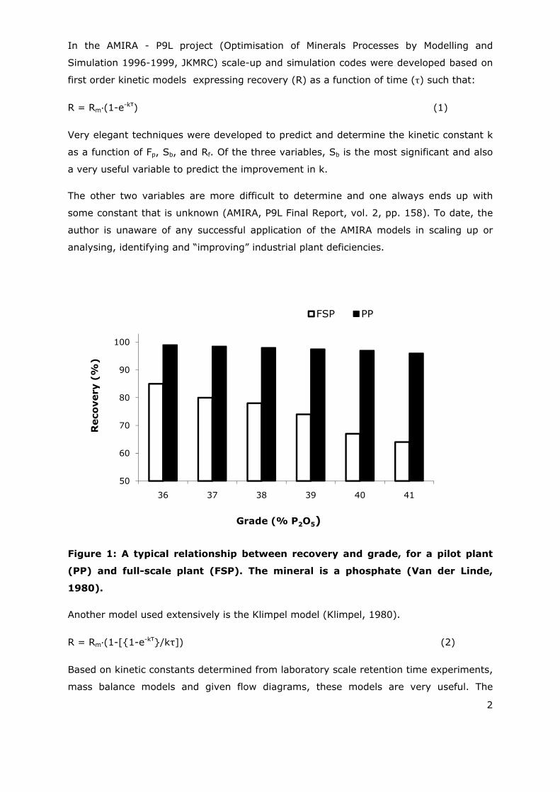
Figure 1 shows grade-recovery data for a pilot plant (black bar) and corresponding
industrial scale (empty bar) phosphate plant in South Africa (Van der Linde, 1980),
where recovery on the full-scale plant is significantly lower than that on the pilot plant.
Although this data might be 25 years old, the conditions and performance are still the
same and the main reason for this seems to be a lack of understanding of the macro-
processes. In some cases only the metallurgical scale-up was performed, because of a
lack of understanding of the hydrodynamics and in other cases the hydrodynamics were
adjusted without understanding the effects on the metallurgy. When referring to the
principles of flotation, metallurgists and engineers often refer to “suppressed turbulence”
and “high agitation” without having an idea how to quantify these requirements. Even in
the basic design, manufacturers seem to contradict the fundamental principles to meet
the requirements of aeration and suspension, e.g. to ensure proper aeration and solid
suspension, manufacturers would design a machine with a low aspect ratio and with
increase rotational speed, thereby threatening froth stability.
2
In the AMIRA - P9L project (Optimisation of Minerals Processes by Modelling and
Simulation 1996-1999, JKMRC) scale-up and simulation codes were developed based on
first order kinetic models expressing recovery (R) as a function of time (τ) such that:
R = Rm (1-e-kτ) (1)
Very elegant techniques were developed to predict and determine the kinetic constant k
as a function of Fp, Sb, and Rf. Of the three variables, Sb is the most significant and also
a very useful variable to predict the improvement in k.
The other two variables are more difficult to determine and one always ends up with
some constant that is unknown (AMIRA, P9L Final Report, vol. 2, pp. 158). To date, the
author is unaware of any successful application of the AMIRA models in scaling up or
analysing, identifying and “improving” industrial plant deficiencies.
Figure 1: A typical relationship between recovery and grade, for a pilot plant
(PP) and full-scale plant (FSP). The mineral is a phosphate (Van der Linde,
1980).
Another model used extensively is the Klimpel model (Klimpel, 1980).
R = Rm (1-[{1-e-kτ}/kτ]) (2)
Based on kinetic constants determined from laboratory scale retention time experiments,
mass balance models and given flow diagrams, these models are very useful. The
50
60
70
80
90
100
110
36 37 38 39 40 41
Reco
very
(%
)
Grade (% P2O5)
FSP PP
3
difficulty is to predict the effect of hydrodynamic changes, conditioning, froth depth and
liberation on k. Tables 1 & 2 show typical results of some non-metal and metal plants
respectively from statistics gathered by the author at different South African plants.
In these tables, the plants are not identified for confidentiality reasons, but simply
indicated as phosphate, carbonate or fluoride in the non-metal plants and Cu-1, Cu-2
(copper), Zn (zinc), and GM-1, -2, -3 (PGM) in the metal plants.
Table 1: Recovery of valuable products at non-metals plants.
Mineral (Mine) Phosphate Carbonate Fluoride
Pilot Plant Recovery (%) 90 95 90
Main Plant recovery (%) 65 90 73
Revenue loss (MR/y) 100 30 30
Table 2: Recovery of valuable products at metals plants.
Mineral (Mine) Cu-1 Cu-2 Zn GM-1 GM-2 PGM-3
PP performance 87 93 95 92 92 72
FSP performance (%) 76 85 87 80 77 35
Revenue loss (MR/y) 100 30 20 300 100 300
No significant change of mineralogy occurred which might have had a negative impact on
recovery. In some cases the reagent suites have been changed to compensate for the
deficiencies in hydrodynamics. Tables 1 & 2 were compiled over six month data at the
same concentrate grade. The author’s estimates of lost revenue are based on the
difference between the pilot plant (PP) performance and the full-scale plant (FSP)
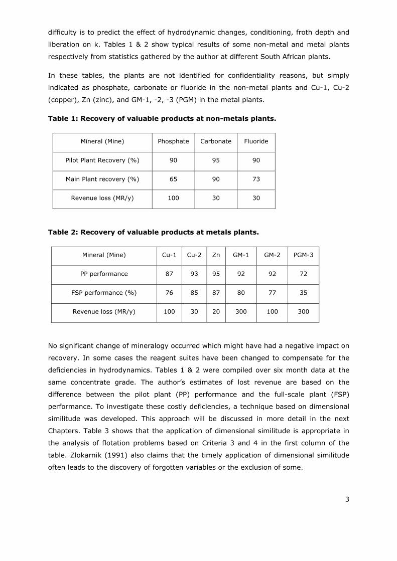
performance. To investigate these costly deficiencies, a technique based on dimensional
similitude was developed. This approach will be discussed in more detail in the next
Chapters. Table 3 shows that the application of dimensional similitude is appropriate in
the analysis of flotation problems based on Criteria 3 and 4 in the first column of the
table. Zlokarnik (1991) also claims that the timely application of dimensional similitude
often leads to the discovery of forgotten variables or the exclusion of some.
4
Table 3: Test of appropriateness for dimensionless analysis of flotation.
1. Are the physics of the basic
phenomenon unknown?
Dimensionless analysis cannot be
applied.
2. Enough is known about the physics of
the basic phenomenon to compile a first,
tentative relevance list.
The resultant dimensionless groups
are unreliable.
3. All the relevant physical variables
describing the problem are known.
The application of dimensionless
analysis is unproblematic.
#
4. The problem can be expressed in terms
of a mathematical equation.
A closer insight into the
dimensionless groups is feasible and
may facilitate in reducing the set of
dimensionless groups.
#
5. A mathematical solution of the problem
exists.
The application of dimensionless
analysis is superfluous.
In the author’s view, another important miss-understanding of the mechanism of
mechanically agitated flotation amongst plant metallurgists and suppliers, which has
fixed the approach to machine and process design over the past years, is that flotation is
the random collision of sinking solid particles and rising bubbles as they move through
the bulk of the machine. In fact flotation is a deliberate attempt to penetrate the
velocity, pressure and tension barriers between particle and bubble.
For this reason, in mechanically agitated machines, the primary impact-collision takes
place in the highly turbulent region at the tip of the rotor and behind the rotor and
between the tip of the rotor and the stator where air changes into small bubbles and the
particles are subjected to large centrifugal forces. Bubble and particles are forced into
one another, penetrating the film between them, attach and then released into the quiet
zone where they float to the froth zone (Schubert and Bischofberger, 1998; Schulze,
1982). Koh et al. (2000), also showed, by means of CFD and applying attachment and
de-attachment models, that attachment is greatest between rotor tip and stator.
Secondary impacts-collision takes place in turbulent eddies further away from the rotor
and to a lesser extent in the boundary layer on the walls of the flotation cell. Sliding-
collision takes place further away but its contribution to collision and attachment is
5
limited. Even in column flotation where no rotor exists, the turbulent conditions, in terms
of Reynolds number around the emerging bubble, as it is ejected from the sparger
nozzle, is almost similar to those experienced on the tip of the rotor.
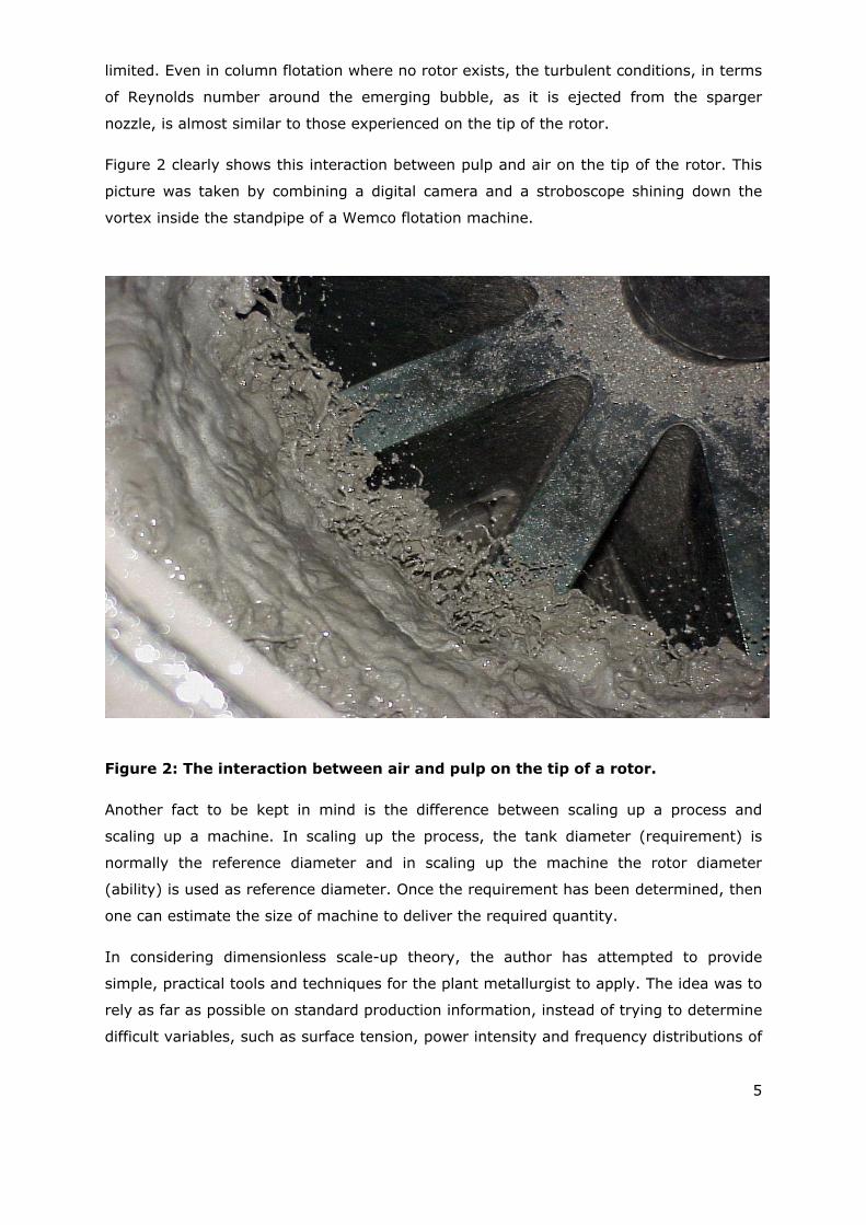
Figure 2 clearly shows this interaction between pulp and air on the tip of the rotor. This
picture was taken by combining a digital camera and a stroboscope shining down the
vortex inside the standpipe of a Wemco flotation machine.
Figure 2: The interaction between air and pulp on the tip of a rotor.
Another fact to be kept in mind is the difference between scaling up a process and
scaling up a machine. In scaling up the process, the tank diameter (requirement) is
normally the reference diameter and in scaling up the machine the rotor diameter
(ability) is used as reference diameter. Once the requirement has been determined, then
one can estimate the size of machine to deliver the required quantity.
In considering dimensionless scale-up theory, the author has attempted to provide
simple, practical tools and techniques for the plant metallurgist to apply. The idea was to
rely as far as possible on standard production information, instead of trying to determine
difficult variables, such as surface tension, power intensity and frequency distributions of
6
the bubbles, all the time assuming constant mineralogy, chemistry, liberation and flow
diagram.
With these issues in mind the author will consider the following hypothesis in this thesis:
Scaled-up froth flotation processes perform significantly worse than expected in the
South African metallurgical industries, owing to the lack of understanding of the correct
scale-up procedures. This can be improved considerably by enforcing dimensional
similitude between laboratory or pilot scale experiments and industrial scale flotation
plants.
The hypothesis will be examined by pursuing the following specific objectives:
Demonstrate that scaled-up flotation plants in the South African industries
perform worse than expected based on laboratory results.
Propose a methodology based on dimensional similitude to improve the scale-up
of flotation plants.
Demonstrate the validity of the methodology via industrial case studies.
The thesis is organised as follows. First the basic concepts behind the dimensional
similitude of flotation systems and the results from a literature study are considered in
Chapter 2. This is followed by a full dimensional analysis of a flotation process, as well as
the derivation of the transformation number for hollow stirrers, a dimensionless form of
the kinetic constant and a schedule of dimensionless numbers for the characterization of
flotation processes in Chapter 3. In Chapter 4, the hydrodynamics of the Wemco
flotation cells are investigated by means of computational fluid dynamics. In Chapters 5
and 6, it is shown that flotation systems from a phosphate and a PGM plant perform
worse than expected on the basis of laboratory-scale results and that this discrepancy in
performance could be reduced substantially by improvements based on the principles of
dimensional similitude. In Chapter 7 a new scale-up methodology is proposed and a
discussion of the difference between literature and this thesis. The thesis ends with
Chapter 8 where the conclusions of the investigation are summarized.
Appendixes 1 to 5 are additional examples of the application of the schedule of
dimensionless numbers, while Appendix 6 demonstrates the use of dimensionless
numbers in specifying different minerals and processes. Appendix 7 gives a detail
analysis of the rest of the dimensionless numbers for a flotation process and Appendix 8
shows the new scale-up algorithm.
7
CHAPTER 2: A LITERATURE REVIEW ON DIMENSIONAL ANALYSIS AND SCALE-UP OF FLOTATION.
2.1. Dimensional analysis and dimensionless numbers.
In studying the literature it was found that the published material can be divided into
two groups and the rest of this document will be discussed under these two headings.
These two groups are:
Those that have attempted to apply the techniques of dimensional analysis to
flotation, and
Those who utilised dimensionless groups to demonstrate the relationship between
these groups and flotation performance.
In engineering the application of fluid mechanics in designs make use, to a large extent,
of empirical results from a lot of experiments. This data is often difficult to present in a
readable form. Even from graphs it may be difficult to interpret. Dimensional analysis
provides a strategy for choosing relevant data and how it should be presented. This is a
useful technique in all experimentally based areas of engineering. If it is possible to
identify the factors involved in a physical situation then dimensional analysis can form a
relationship between them. The resulting expressions may not at first sight appear
rigorous, but these qualitative results converted to quantitative forms can be used to
obtain any unknown factors from experimental results. (Sleigh and Noakes, 2009).
Ruzicka (2008) stated that dimensionless numbers are useful in that:
They reduce the number of variables needed for description of the problem
thereby reducing the amount of experimental data and at making correlation.
They simplify the governing equations.
They produce valuable scale estimates, whence order of magnitude estimates of
important physical quantities.
When properly formed, they have clear physical interpretation and thus
contribute to the physical understanding of the phenomenon under study.
8
2.2. Dimensions and units.
Any physical situation can be described by certain familiar properties e.g. length,
velocity, area, volume, acceleration, etc. The following columns give an explanation of
the difference between quantity, units and dimensions.
Quantity Units Dimensions
Velocity m/s LT-1
Force kg m/s2 MLT-2
Dimensions are properties which can be measured. Units are the standard elements used
to quantify these dimensions. In dimensional analysis we are only concerned with the
nature of the dimension i.e. its quality not its quantity. All properties can be represented
with L, T, M and temperature. (Sleigh and Noakes, 2009).
2.3. Dimensional homogeneity.
Any equation describing a physical situation will only be true if both sides have the same
dimensions. That is it must be dimensionally homogeneous. (Sleigh and Noakes, 2009).
For example:
The flow through a weir is:
0.66 · B · 2 · g H . (3)
The SI units of the left hand side are m3s-1. The units on the right hand side are equal
to:
m(ms-2)1/2m3/2 = m3s-1 (4)
2.4. Typical results from a dimensional analysis.
The result of performing dimensional analysis on a physical problem is a single equation.
This equation relates all of the physical factors involved to one another. For example, if
we want to find the force on the blade of a propeller we must first decide what might
influence this force. It would be reasonable to assume that the force Fo, depends on the
following physical properties:
9
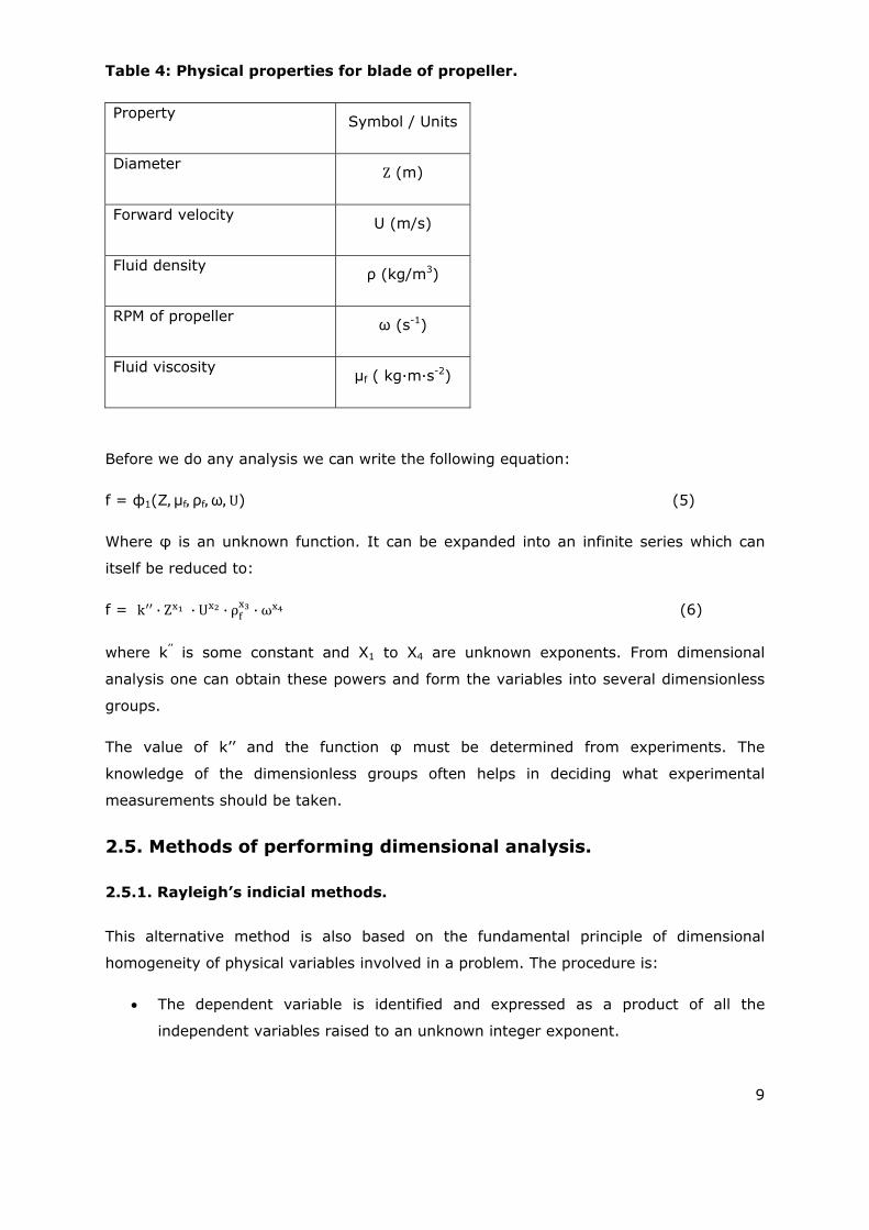
Table 4: Physical properties for blade of propeller.
Property Symbol / Units
Diameter Ζ (m)
Forward velocity U (m/s)
Fluid density ρ (kg/m3)
RPM of propeller ω (s-1)
Fluid viscosity μf ( kg·m·s-2)
Before we do any analysis we can write the following equation:
f = ф1(Z, μf, ρf, ω, U) (5)
Where φ is an unknown function. It can be expanded into an infinite series which can
itself be reduced to:
f = k · Z · U · ρ · ω (6)
where k’’ is some constant and X1 to X4 are unknown exponents. From dimensional
analysis one can obtain these powers and form the variables into several dimensionless
groups.
The value of k’’ and the function φ must be determined from experiments. The
knowledge of the dimensionless groups often helps in deciding what experimental
measurements should be taken.
2.5. Methods of performing dimensional analysis.
2.5.1. Rayleigh’s indicial methods.
This alternative method is also based on the fundamental principle of dimensional
homogeneity of physical variables involved in a problem. The procedure is:
The dependent variable is identified and expressed as a product of all the
independent variables raised to an unknown integer exponent.
10
Equating the indices of n fundamental dimensions of the variables involved, n
independent equations are obtained.
These n equations are solved to obtain the dimensionless groups.
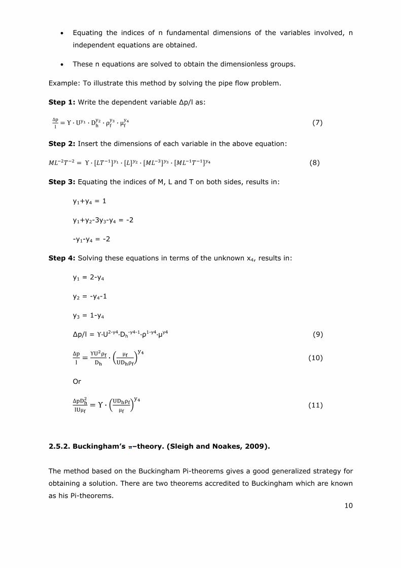
Example: To illustrate this method by solving the pipe flow problem.
Step 1: Write the dependent variable ∆p/l as:
∆ · U · D · ρ · µ (7)
Step 2: Insert the dimensions of each variable in the above equation:
· · · · (8)
Step 3: Equating the indices of M, L and T on both sides, results in:
y1+y4 = 1
y1+y2-3y3-y4 = -2
-y1-y4 = -2
Step 4: Solving these equations in terms of the unknown x4, results in:
y1 = 2-y4
y2 = -y4-1
y3 = 1-y4
∆p/l = U2-y4 Dh-y4-1 ρ1-y4 μy4 (9)
∆ U
D· µ
UD (10)
Or
∆ D
Uµ· UD
µ (11)
2.5.2. Buckingham’s –theory. (Sleigh and Noakes, 2009).
The method based on the Buckingham Pi-theorems gives a good generalized strategy for
obtaining a solution. There are two theorems accredited to Buckingham which are known
as his Pi-theorems.
11
1st -theorem:
A relationship between m variables can be expressed as a relationship between m-n
non-dimensional groups of variables where n is the number of fundamental dimensions
required to express the variables. If a physical problem can be expressed as:
Ф2(Q1, Q2, Q3,………..Qm) = 0 (12)
Then according to the above theorem, this can also be expressed as:
ф , , , … … . , 0 (13)
In most fluids n = 3.
2nd theorem:
Each -group is a function of n governing or repeating variables plus one of the
remaining ones. Both Buckingham’s method and Rayleigh’s method of dimensional
analysis determine only relevant independent parameters of a problem, but not the
exact relationship between them.
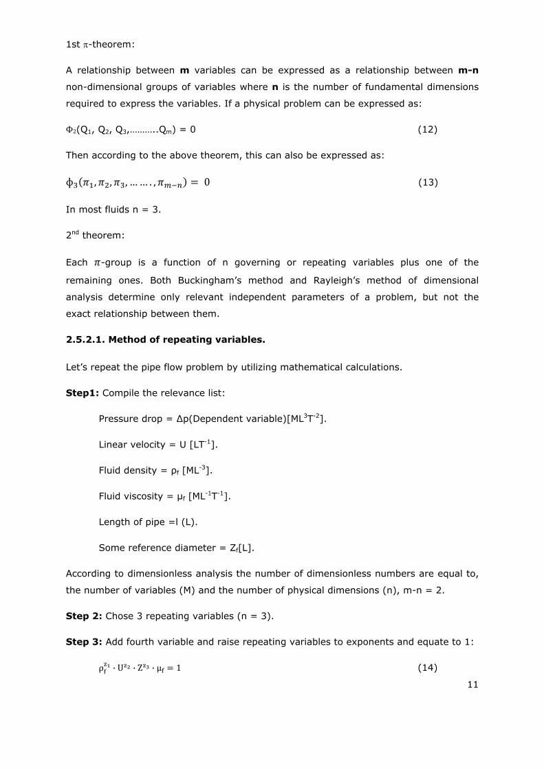
2.5.2.1. Method of repeating variables.
Let’s repeat the pipe flow problem by utilizing mathematical calculations.
Step1: Compile the relevance list:
Pressure drop = ∆p(Dependent variable)[ML3T-2].
Linear velocity = U [LT-1].
Fluid density = ρf [ML-3].
Fluid viscosity = μf [ML-1T-1].
Length of pipe =l (L).
Some reference diameter = Zf[L].
According to dimensionless analysis the number of dimensionless numbers are equal to,
the number of variables (M) and the number of physical dimensions (n), m-n = 2.
Step 2: Chose 3 repeating variables (n = 3).
Step 3: Add fourth variable and raise repeating variables to exponents and equate to 1:
ρ · U · Z · µ 1 (14)
12
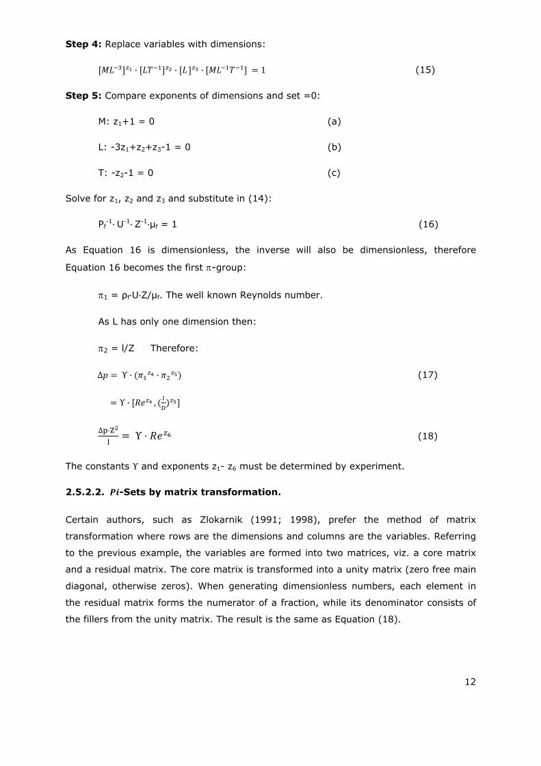
Step 4: Replace variables with dimensions:
· · · 1 (15)
Step 5: Compare exponents of dimensions and set =0:
M: z1+1 = 0 (a)
L: -3z1+z2+z3-1 = 0 (b)
T: -z2-1 = 0 (c)
Solve for z1, z2 and z3 and substitute in (14):
Ρf-1 U-1 Z-1 μf = 1 (16)
As Equation 16 is dimensionless, the inverse will also be dimensionless, therefore
Equation 16 becomes the first -group:
1 = ρf U Z/μf. The well known Reynolds number.
As L has only one dimension then:
2 = l/Z Therefore:
∆ · · (17)
· ,
∆ Z (18)
The constants and exponents z1- z6 must be determined by experiment.
2.5.2.2. -Sets by matrix transformation.
Certain authors, such as Zlokarnik (1991; 1998), prefer the method of matrix
transformation where rows are the dimensions and columns are the variables. Referring
to the previous example, the variables are formed into two matrices, viz. a core matrix
and a residual matrix. The core matrix is transformed into a unity matrix (zero free main
diagonal, otherwise zeros). When generating dimensionless numbers, each element in
the residual matrix forms the numerator of a fraction, while its denominator consists of
the fillers from the unity matrix. The result is the same as Equation (18).
13
2.6. Choice of variables.
2.6.1. List of variables.
Zlokarnik (1991) calls it the relevance list and both Zlokarnik and Ruzicka state that it
must comply with the following requirements:
They must be relevant.
They must be independent.
The list must be complete.
The choice is highly subjective and needs profound understanding of the problem,
experience with the use of dimensionless analysis, intuition and luck. A general rule for
independence is that if there are m variables then these variables will be independent, if
there is no combination of these variables that will result in an additional variable with
the same dimensions of any of the m variables. Examples of these dependent variables
are:
P ≈ ρ ω3 d5, vt = ω d/2, = μp/ρp and q ≈ ω d3 therefore:
P, vt, and μf, ρf, ω, and d cannot be part of a relevance list at the same time.
2.6.2. Repeating variables.
Repeating variables are those which we think will appear in all or most of the groups
and are a influence on the problem. There is considerable freedom allowed in the choice
of the repeating variables although there are certain rules which should be followed.
These rules are:
From the second theorem there should be n repeating variables.
When combined, these repeating variables must contain all the dimensions (Mass,
Length and Time).
A combination of the repeating variables must not form a dimensionless group.
All the repeating variables do not have to appear in all groups.
The repeating variables should be chosen to be measurable in an experimental
investigation. They should be of major importance to the designer. For example
pipe diameter is more useful and measurable than roughness.
14
In fluid it is usually possible to choose density, velocity and some reference diameter as
repeating variables. This freedom of choice results in there being many different -
groups which can be formed - and all are valid. There is not really a wrong choice.
2.7. Wrong choice of physical properties.
If, when defining the problem, extra unimportant variables are introduced then extra л-
groups will be formed. They will play very little role influencing the physical behaviour of
the problem concerned and should be identified during experimental work. If and
important/influential variable was missed then a -group would be missing. Experimental
analysis based on these results may miss significant behavioural changes. It is therefore
important that the initial choice of variables is carried out with great care.
2.8. Similitude.
Dimensionless numbers can be grouped into geometrical groups, kinematic groups and
dynamic groups. A model is said to have similitude with the real application when the
two share geometric, kinematic and dynamic similarity.
2.9. Dimensional analysis and flotation.
To demonstrate this technique in flotation it was decided to use an example by Zlokarnik
(1972). Although this is a relative old example the principles and arguments are still the
same. This is a very good example of the techniques, mathematics and arguments
followed to eliminate certain variable in an effort to define the transformation
dimensionless group.
2.9.1. Scale-up of flotation cells with stirrers and separate air intake.
Zlokarnik (1972) presented this lecture to the German expert commission on ore
dressing in 1972 and is a very good example of the application of dimensional analysis
on flotation. It is reproduced here to demonstrate the thinking in eliminating and
combination of certain variables. Since the flow state of a flotation cell with a stirring
apparatus depends largely on stirring conditions, we will select the diameter of the
stirrer d, as the characteristic apparatus measurements to determine all other geometric
measurements such as D/d, H/d, h/d, b/d etc, where D is the diameter of the container,
H* is the level of the liquid, h* is the distance of the stirrer from the bottom and b is the
blade height of the stirrer. The material system is completely described by the average
particle size δ, the solid content of materials in suspension φs, the density of the solid
and liquid ρs and ρf, the kinetic viscosity , and the surface tension σ. The material
values of the gaseous phase may be considered as negligible. The relevant kinematic
15
variables are the rotational rate of the stirrer ω, the air throughput qa and the
gravitational constant g. For further analysis we will combine density and gravity such
that g∆ρ=g ρf (ρs-ρf). The complete function with relevant variables is:
f1 (d, δ, φs , ρs, ρf, , σ, ω, qa, g∆ρ ) = 0 (19)
The interpretation of this relationship based on the theory of similarity leads to the
following set of (10-3) = 7 known dimensionless groups.
f2 (Fr, Re, We, Qa, ρs/ρf, δ/d, φs) = 0 (20)
The Weber number or characteristic value is now transformed into a simple material
characteristic value by a special adapted combination with Fr and Re.
We* = We/(Fr’ Re4)0.33 = ρf (g ∆ρ ν )0.33(σ ρf0.33) (21)
From (18) we may then derive:
f3 (Fr’,Re, Qa, δ/d, We*, ρs/ρf, φs) = 0 (22)
The last three characteristic values in (21) are simple material variables which numeric
values are not changed by a scale transformation within the same material system. The
same applies to the quotient ∆p/ρp in Fr’. The following thus applies to scale
transformation.
f4 (Fr, Re, Qa, δ/d) = 0 (23)
With ∆p/ρp, We* and ρs/ρf = idem. (Idem indicates an identical numerical value).
Relationship (23) seems not to have been the subject of research either in flotation
technology or in stirring technology. We may nevertheless assume that the flow state
here differs only marginally from the flow state with automatic suction stirrers for which
exhaustive research is available in terms of stirring technology (Zlokarnic M and Judat H
1969).
2.9.2. Scale-up of flotation cell with an automatic suction stirrer.
The tube stirrer is an automatic suction hollow stirrer used for adding gas to liquids,
while the propeller stirrer attached to the same shaft underneath the tune stirrer was
intended to churn up solid material from the bottom of the container.
For automatic suction stirrers, air throughput qa is no longer an independent variable as
it is dependent on ω and d as well as dimensions of the air channel. For a geometrically
similar scale transfer the new valid function is:
16
f5 (Fr, Re, δ/d) = 0 (24)
This π-space has already been investigated in the stirring technology, by Zlokarnik and
Judat (1969), by determining the so called churning characteristic of the stirrer. The
measurements determined the smallest rotational speed of the stirrer at which all solid
particles are in motion (not floating). During these experiments these two researchers
proved that the critical Reynolds and Froude number exist and can be combined into a
critical Froude number:
Frcrit = const ∆ρ/ρp δ/d 0.33 φs0.33
Through a process of eliminating of small ratios with low exponent numbers (δ/d)0.33 and
for a similar scale transfer (∆ρ/ρp, φs = idem), Zlokarnik and Judat concluded that the
transfer rule for a flotation cell with an automatic stirrer with geometrically similar shape
is given by
Fr ~ ω2 d = idem. (25)
The discovery that in the turbulent flow range (Re > 104) the flow state in a solid/liquid
system without air input can also be described by Froude’s number alone was confirmed
by Kneule and Weinspach with extensive measurements. Zlokarnic and Judat also
proved that the output P as the We = P/ρp ω3 d5, and Ne = f(Fr) and Qa = f(Fr), results in
Ne = f(Qa). This automatically implies that the transformation is:
Fr = ω2 d/g = idem and Qa = qa/ω d3 = idem. (26)
2.9.3. Technical stirring conclusions derived from the transformation criterion
Fr = idem.
Now that Fr has been identified as the relevant transformation criteria for mechanically
agitated machines based on the theory of similarity, the technical stirring aspects arising
from it must be discussed.
2.9.3.1. Stirring output in cells with separate air intake.
Zlokarnik(1972) continued to prove that the power output in a mechanically agitated
machine with separate air intake based on the Newton number is:
Ne = f(Qa)
This was made possible by extending the relevance list in Equation (20) by adding the
Newton number and then eliminating dimensionless numbers through the following
arguments:
17
Experiments have shown that a volume portion solid matter in liquid containing
up to 25%-30% solids in suspension, the characteristic values of ρs/ρp, δ/d and φs
are adequately considered if Newton number is formed not with the density of the
liquid but with the density of the suspension.
In the turbulent flow range Re > 104. The Reynolds number has no effect on the
Newton number. Even the surface tension and thus the Weber number barely
affects the Newton number.
This means that Ne = f(Fr,Qa) and for a scaled transformation according to Fr= idem and
Qa = idem then Ne = idem.
2.9.3.2. Stirring output and gas throughput with an automatic suction stirrer.
For automatic suction stirrers both the stirring output and the gas throughput are
functions of the Froude number. But as Qa is strongly influenced by the head of liquid
above the stirrer then Qa = f(Fr d/H*). Since both Ne and Qa are functions of the Froude
characteristic value then both these functions can be represented in the so-called
parameter format Ne = f(Qa) which illustrates the parallels to string output with a
separate air intake.
2.9.4. Stirrer volume related output and the criterion Fr=idem.
Even though it is based on fluid material systems liquid/liquid and liquid/gaseous, the
constant volume related stirring output P/V = constant is often invoked as a standard
value for dimensioning stirring chemical processes. It should not be failed to be observed
that this variable is particularly ill-suited for dimensioning flotation cells. It can be shown
(Zlokarnik, 2006) that when applying the scaling transformation, then:
(P/Qt)actual = [(P/Qt)model.(Sc)1/2] Where Sc = scale factor. (27)
This is because the scale –up parameter for a stirrer is the Fr number and especially Fr3/2
which equals (P/Qt).d0.75. Today’s experience with flotation cells show that
transformation scales exceed 1:10 ratios, and therefore does not support the
requirement P/Qt = idem. (Zlokarnic, 1972).
2.9.5. Interpretive data of a few flotation cells.
Zlokarnik(1972) compared the data of a few industrial designs to test how far these
interpretative criteria fall from practical technology and concluded that these designs did
18
not maintain geometric similarity with a wide variation in Froude number and aeration
number. Zlokarnik found that the Wemco design is largely based on:
P/Qt = idem or ω3 d2 idem
2.9.6. Summary of Zlokarnik and Judat’s work.
A consequent analysis of flow patterns in flotation cells with stirrer based on similarity
was carried out by Zlokarnic and Judat. A comparison of the resulting relationships with
the recent findings of mixing research lead to the scale-up conditions:
Fr = ω2 d/g = idem and Qa = qa /ω d3 = idem. Identical materials and geometric
similitude supposed.
Consequently, the stirrer has to be dimensioned according to ω2 d = idem and not as
previously on the basis of constant tip speed vt = ω d.
The air throughput has to be scaled up according to:
Qa Fr1/2 = qa (d2.5 g0.5) ~ qa/(Ac d1/2) = idem. (28)
Not as previously thought on the condition of constant surface throughput qa/Ac. For the
power input, these conditions Fr, Qa = idem have the consequence that in scale-up the
power number Ne = ρp ω3 d5 retains it numerical value. In the case of automatic suction
stirrers, the condition Fr = idem leads to Qa = idem.
A further consequence of Fr = idem as scale-up criteria is that the power per unit
volume, P/Qt increases with the square root of the scale.
Dimensional analysis either works or fails. When it works it gives good or bad results.
When it gives good results, either the choice of variables is correct or the extra variables
are eliminated. When it fails, it is either by logical contradiction (dimension of left hand
side not equal to right hand side) or by insolubility, since extra variables bring more
equations but not new dimensions (Ruzicka, 2008)
2.10. Flotation performance and dimensionless numbers.
Many publications are available on researchers such as Deglon et al. (1999; 2000) and
Rodrigues et al. (2001), who produced very interesting results of flotation performance
based on dimensionless numbers without performing dimensionless analysis or scale-up
analysis, but have chosen these specific numbers based on their knowledge of the
flotation process.
19
Rodriques et al. (2001) probably produced the best evidence that recovery in a
mechanically agitated flotation process is a function of Reynolds number, Froude
number and power number. Rodriques’s results were based on very small
laboratory scale experiments with very low Reynolds numbers and power
numbers. These results showed distinct maximums in recovery at Reynolds
number = 10000, Froude number = 1 and power number > 0.55.
Deglon et al. (2000) evaluated industrial machines in the South African platinum
industry and also found a large variation in rotor tip Reynolds number, aeration
numbers, power numbers and Froude numbers. Deglon et al. (2000) did not try
to give an explanation for these large variations.
Mavros (1992) suggested that these variations are functions of rotor aspect ratio,
which is not considered in the determination of the power number and aeration
number, and the large variations in rotor tip Reynolds number is a function of the
ratio of particle size to tank diameter between designs.
Newell and Grano (2006; 2007) found that the scale-up of the flotation rate
constant can be achieved by maintaining a constant bubble surface area flux as
well as maintaining ω3d. A constant ω3d enable the measurement of mean energy
dissipation (W/kg). The problem with these experiments is that they were all
executed on relative small cells.
Gorain et al. (1996) showed that a linear relationship exists between kinetic
constant and bubble surface area flux and that it is independent of the type of
impellor. This finding does have potential as a scale-up tool. Gorain et al. (1997)
also developed very useful tools for bubble surface flux:
Sb = 134 ( vt)0.33 Jg 0.75 ÅRa ‐0.12 P80 ‐0.4
Looking at experimental and predicted results then this model predicts very
accurate results. These variables are also easy measureable factors.
2.11. Summary.
The results from this literature study can be summarized as follows:
2.11.1. Dimensionless analysis for scale-up in flotation is limited to a few authors, while
the use of dimensionless numbers to describe flotation performance is more
common.
20
2.11.2. While Deglon et al. (2000), Gorain et al. (1996), and Rodriques et al. (2001)
concentrated on energy dissipation, rotor tip velocity and Reynolds number,
Froude number, aeration and power number to prove a relationship between
these variables and recovery or kinetic constant, only Zlokarnik (1972)
attempted to derive the transformation number, for mechanism scale-up, with
dimensional analysis.
2.11.3. Both Zlokarnic, Deglon et al. (2000) and Gorain et al. (1999), concluded that
industrial designs, both external and self-aerated, do not comply with the basic
Froude number as transformation scale-up number but rather a combination of
Reynolds and Froude in the form: Re Fr0.5 = idem. For self-aerating machines
the parameters Qa = idem and Ne = idem also apply.
Interesting to note that the scale-up number Re Fr0.5 = ρp ω3 d5/μp √g ω D2.5 is a
special form of the power number.
2.11.4. Very little information is available on actual application and success of the scale-
up numbers from pilot plant to full scale plant as well as the identification of
deficiencies and prediction of improvements.
In the following chapter the author will perform a dimensional analysis with all the
possible macro hydrodynamic variables and with the emphasis on a new transformation
equation, a dimensionless kinetic constant and a schedule of dimensionless numbers as
a simple tool for the plant metallurgist to analyze and identify deficiencies in his/her
plant.
21
CHAPTER 3: DIMENSIONAL ANALYSIS OF A FLOTATION PROCESS.
3.1. Dimensional analysis.
In this analysis the flotation process will be divided into the following characteristic
operations:
Machine characteristics.
Kinetic characteristics.
Process characteristics.
During this analysis the author will endeavour to define the transformation numbers for
machine scale-up, the kinetic model in dimensionless form for performance prediction
and a schedule of dimensionless numbers to characterize the process with mechanical
agitated machines.
Fundamentally, dimensional similitude, by way of the -theory, offers the only means of
dealing with problems that cannot be formulated mathematically and that two processes
may be considered completely similar if they take place in similar geometrical space and
if all the dimensionless numbers necessary to describe them, have the same numerical
values (Zlokarnic, 1991). This fundamental approach forms the basis for the rest of this
thesis.
From §2.5.3 the arguments state that if a variable y’, depends upon a number of
independent variables Q1, Q2, Q3...Qn, then they may be arranged in the following
generic functional form:
y’ = f1(Q1, Q2, Q3…Qn) (29)
If all n variables can be expressed by m fundamental dimensional units, then they may
be grouped in (n-m) dimensionless -terms. To compile these dimensionless groups for a
froth flotation system, the variables indicated in Figure 3 and summarised in Table 6
were defined.
22
3.2. Relevance list and linear independence.
To compile the relevance list one must have a clear understanding of what one wants to
achieve. This will help in identifying unwanted and unnecessary variables that will
complicate the experimental setup. In this case the relevant list will include all the
variables that can be identified and the rules for the selection of variables (§ 2.6.1) will
be applied for each characteristic operation.
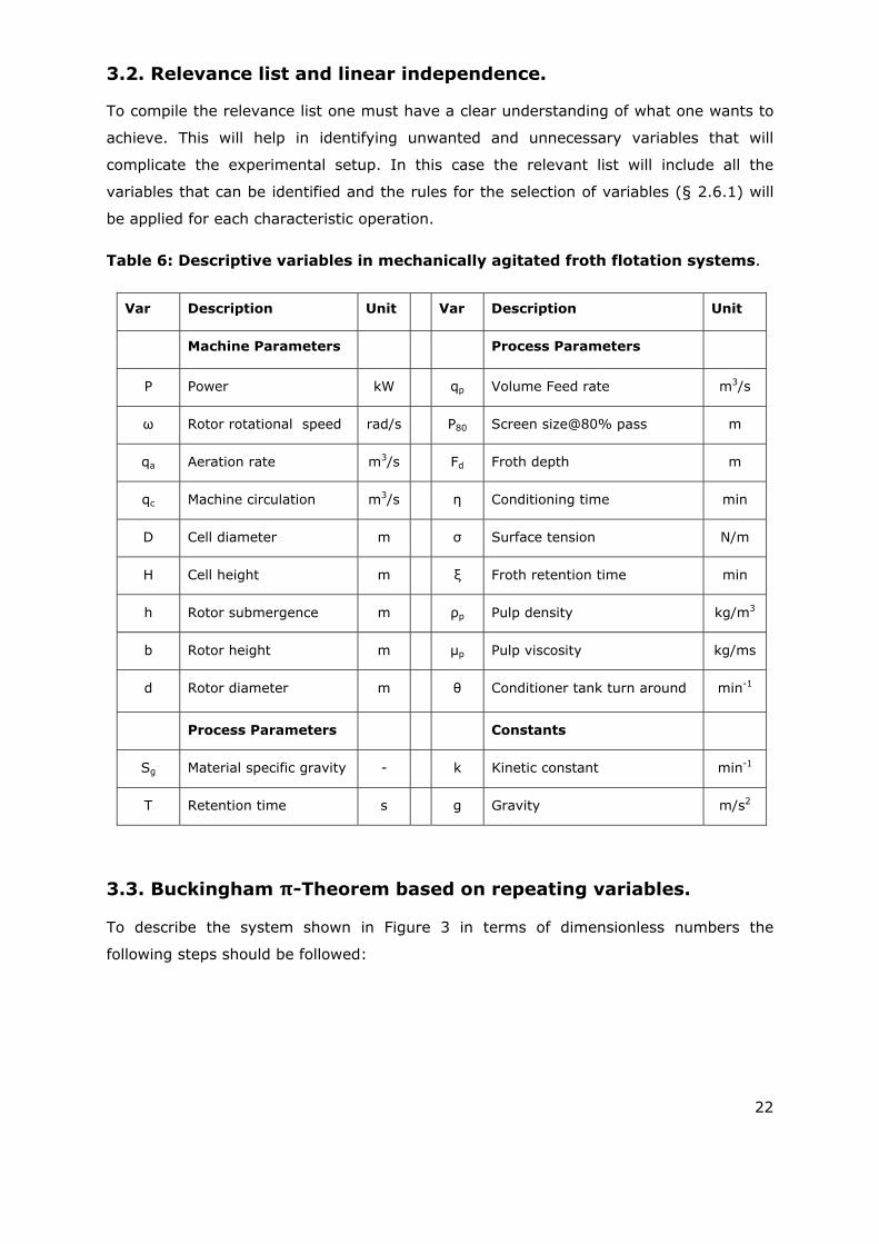
Table 6: Descriptive variables in mechanically agitated froth flotation systems.
Var Description Unit Var Description Unit
Machine Parameters Process Parameters
P Power kW qp Volume Feed rate m3/s
ω Rotor rotational speed rad/s P80 Screen size@80% pass m
qa Aeration rate m3/s Fd Froth depth m
qc Machine circulation m3/s η Conditioning time min
D Cell diameter m σ Surface tension N/m
H Cell height m ξ Froth retention time min
h Rotor submergence m ρp Pulp density kg/m3
b Rotor height m µp Pulp viscosity kg/ms
d Rotor diameter m θ Conditioner tank turn around min-1
Process Parameters Constants
Sg Material specific gravity - k Kinetic constant min-1
T Retention time s g Gravity m/s2
3.3. Buckingham -Theorem based on repeating variables.
To describe the system shown in Figure 3 in terms of dimensionless numbers the
following steps should be followed:
23
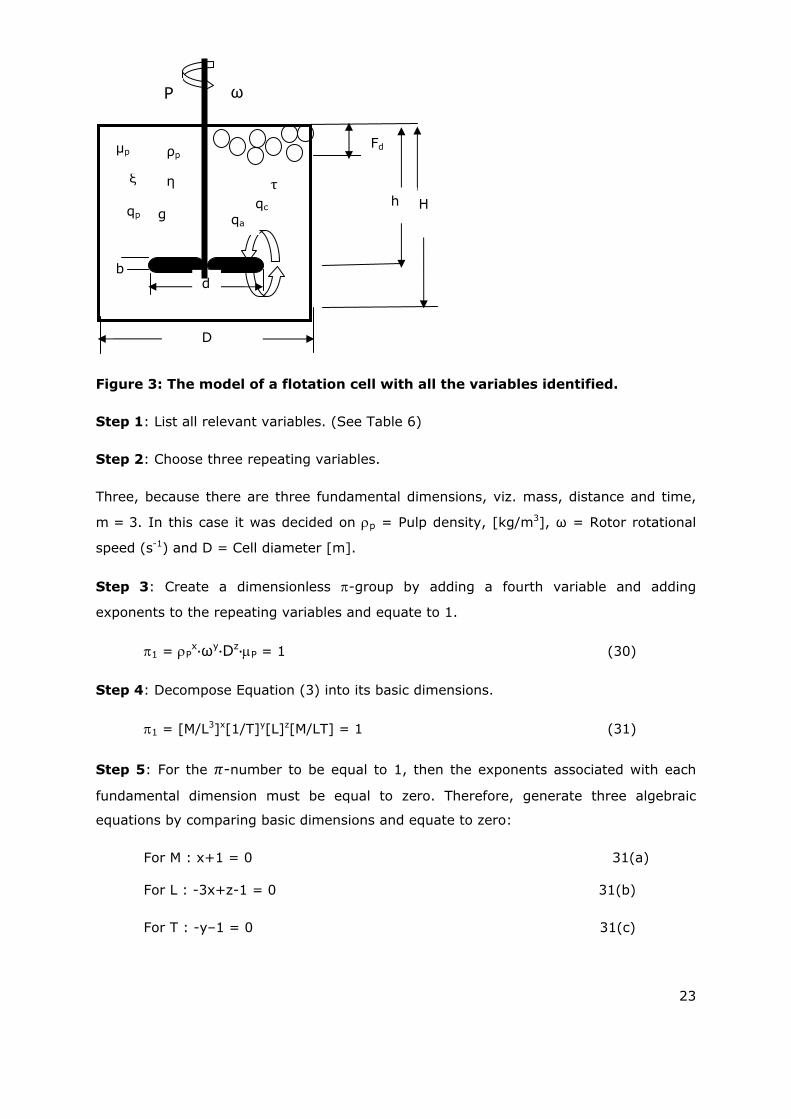
Figure 3: The model of a flotation cell with all the variables identified.
Step 1: List all relevant variables. (See Table 6)
Step 2: Choose three repeating variables.
Three, because there are three fundamental dimensions, viz. mass, distance and time,
m = 3. In this case it was decided on p = Pulp density, [kg/m3], ω = Rotor rotational
speed (s-1) and D = Cell diameter [m].
Step 3: Create a dimensionless -group by adding a fourth variable and adding
exponents to the repeating variables and equate to 1.
1 = Px ωy Dz P = 1 (30)
Step 4: Decompose Equation (3) into its basic dimensions.
1 = [M/L3]x[1/T]y[L]z[M/LT] = 1 (31)
Step 5: For the -number to be equal to 1, then the exponents associated with each
fundamental dimension must be equal to zero. Therefore, generate three algebraic
equations by comparing basic dimensions and equate to zero:
For M : x+1 = 0 31(a)
For L : -3x+z-1 = 0 31(b)
For T : -y–1 = 0 31(c)
ω P
ρp
ξ η
µp
qa qc qp
D
H
Fd
h
d
g
b
τ
24
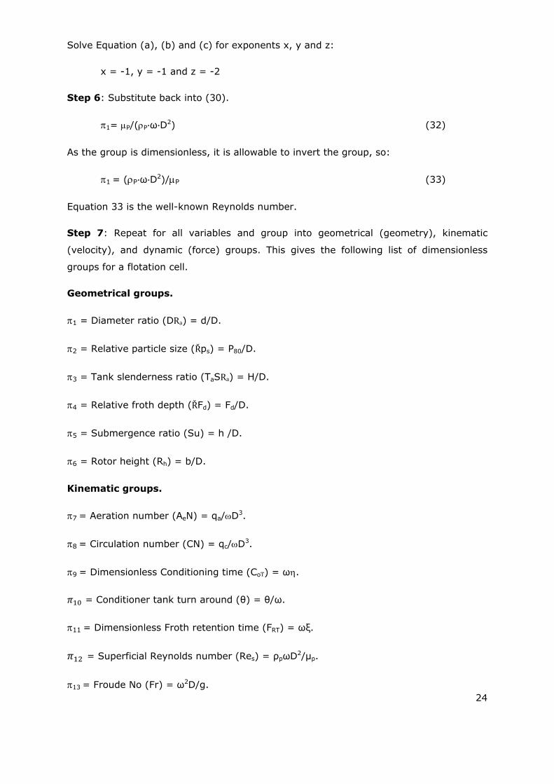
Solve Equation (a), (b) and (c) for exponents x, y and z:
x = -1, y = -1 and z = -2
Step 6: Substitute back into (30).
1= P/(P ω D2) (32)
As the group is dimensionless, it is allowable to invert the group, so:
1 = (P ω D2)/P (33)
Equation 33 is the well-known Reynolds number.
Step 7: Repeat for all variables and group into geometrical (geometry), kinematic
(velocity), and dynamic (force) groups. This gives the following list of dimensionless
groups for a flotation cell.
Geometrical groups.
1 = Diameter ratio (DRa) = d/D.
2 = Relative particle size (Řps) = P80/D.
3 = Tank slenderness ratio (TaSRa) = H/D.
4 = Relative froth depth (ŘFd) = Fd/D.
5 = Submergence ratio (Su) = h /D.
6 = Rotor height (Rh) = b/D.
Kinematic groups.
7 = Aeration number (AeN) = qa/D3.
8 = Circulation number (CN) = qc/D3.
9 = Dimensionless Conditioning time (CoT) = ω.
= Conditioner tank turn around (θ) = θ/ω.
11 = Dimensionless Froth retention time (FRT) = ωξ.
= Superficial Reynolds number (Res) = ρpωD2/µp.
13 = Froude No (Fr) = ω2D/g.
25
Dynamic groups.
14 = Tank power number (TaPNo) = P/(p3D5).
= Weber number (We) = ρpω2d3/σ.
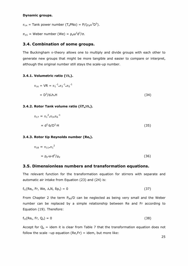
3.4. Combination of some groups.
The Buckingham -theory allows one to multiply and divide groups with each other to
generate new groups that might be more tangible and easier to compare or interpret,
although the original number still stays the scale-up number.
3.4.1. Volumetric ratio (VRa).
16 = VR = 1-1.3
-1.5-1
= D3/d.h.H (34)
3.4.2. Rotor Tank volume ratio (ŔTaVRa).
17 = 12.3.6
-1
= d2 b/D2 H (35)
3.4.3. Rotor tip Reynolds number (Ret).
18 = 11.12
= ρp ω d2/µp (36)
3.5. Dimensionless numbers and transformation equations.
The relevant function for the transformation equation for stirrers with separate and
automatic air intake from Equation (23) and (24) is:
ft1(Ret, Fr, We, AeN, Řps) = 0 (37)
From Chapter 2 the term P80/D can be neglected as being very small and the Weber
number can be replaced by a simple relationship between Re and Fr according to
Equation (19). Therefore:
ft2(Ret, Fr, Qa) = 0 (38)
Accept for Qa = idem it is clear from Table 7 that the transformation equation does not
follow the scale –up equation (Re,Fr) = idem, but more like:

26
ft3(Ret, Fr, ÅRa, G) = 0 (39)
Where G represents the ratio between full scale plant P80 and tank diameter and pilot
plant P80 and tank diameter. A comparison of industrial designs are shown in Table 7.
Table 7: Comparison of transformation equation for industrial installations.
Machine Dim. Denver
PP
Wemco
21m3
Metso
20m3
O/K
20m3
BQR
50m3
O/K
130m3
Mineral processed NA Phos. Phos. PGM
UG2
PGM
UG2
PGM
UG2
PGM
Mer
Tank Volume M3 0.08 20 20 20 50 130
Tank Diameter m 0.43 3.6 3.25 3.2 4.3 6
Tank Height m 0.41 2.4 3 3.45 4.2 5.2
Submergence m 0.25 0.3 2 2.45 2.7 3.7
Rotor Diameter m 0.22 0.76 0.79 0.75 0.99 1.3
Rotor Height m 0.03 0.76 0.54 o.47 0.645 1.23
RPM r/s 90 18.5 18 19.3 14 10.3
(FSP)p80:(PP)p80 μm 250:250 350:250 150:100 150:100 150:100 150:100
Circulation m3/s 0.003 0.53 1.1 1.16 2.7 3.5
Aeration m3/s 0.0006 o.1 0.167 0.116 0.167 0.33
Power kW 0.56 60 55 65 110 144
Ret - 1.75E6 4.6E6 4.36E6 4.2E6 5.34E6 6.77E6
FrD - 45.5 6.7 6.5 7.1 4.95 3.5
Fr*=Ret FrD )0.25 (106) - 4.5 9.2 7 6.8 8 9.26
Fr* ÅRa-0.2 G0.45 (106) - 3.1 3.3 3.4 3.3 3.4 3.4
According to the result in Table 7 the transformation Fr=idem was not followed and even
though the application was for the same mineral, it seems that the designs complied to a
combination of Ret, Fr0.25, ÅRa-0.2 and G0.45. It seems that the designs average around
FrRGA = Ret Fr0.25 G0.45 ÅRa-0.2 = 3.5x10⁶. Here again the Wemco design did not follow the
theoretical transformation equation of Fr=idem but also FrRGA = idem. In Table 7 the
designs, from the different suppliers, different sizes and different minerals, followed
27
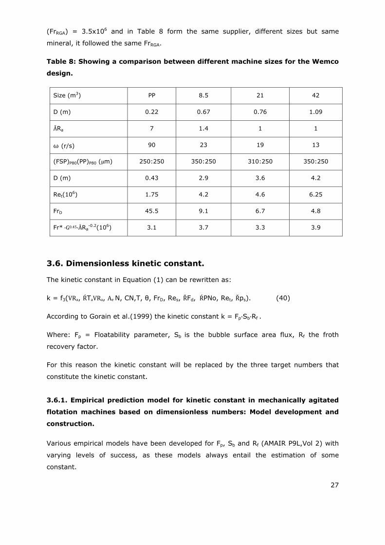
(FrRGA) = 3.5x10⁶ and in Table 8 form the same supplier, different sizes but same
mineral, it followed the same FrRGA.
Table 8: Showing a comparison between different machine sizes for the Wemco
design.
Size (m3) PP 8.5 21 42
D (m) 0.22 0.67 0.76 1.09
ÅRa 7 1.4 1 1
ω (r/s) 90 23 19 13
(FSP)P80(PP)P80 (µm) 250:250 350:250 310:250 350:250
D (m) 0.43 2.9 3.6 4.2
Ret(106) 1.75 4.2 4.6 6.25
FrD 45.5 9.1 6.7 4.8
Fr* G0.45 ÅRa-0.2(106) 3.1 3.7 3.3 3.9
3.6. Dimensionless kinetic constant.
The kinetic constant in Equation (1) can be rewritten as:
k = f3(VRa, ŔTaVRa, Ae N, CN,T, θ, FrD, Res, ŘFd, ŔPNo, Ret, Řps). (40)
According to Gorain et al.(1999) the kinetic constant k = Fp Sb Rf .
Where: Fp = Floatability parameter, Sb is the bubble surface area flux, Rf the froth
recovery factor.
For this reason the kinetic constant will be replaced by the three target numbers that
constitute the kinetic constant.
3.6.1. Empirical prediction model for kinetic constant in mechanically agitated
flotation machines based on dimensionless numbers: Model development and
construction.
Various empirical models have been developed for Fp, Sb and Rf (AMAIR P9L,Vol 2) with
varying levels of success, as these models always entail the estimation of some
constant.
28
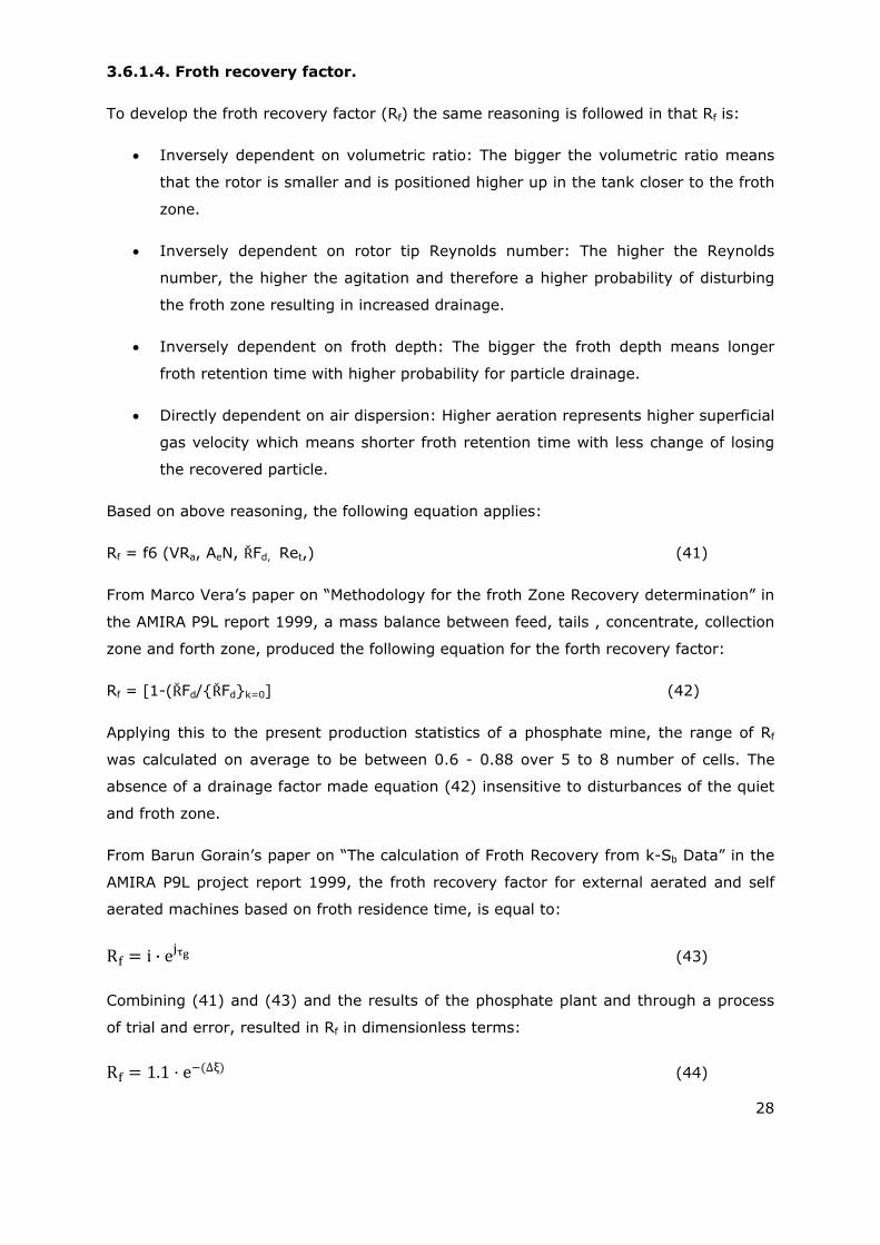
3.6.1.4. Froth recovery factor.
To develop the froth recovery factor (Rf) the same reasoning is followed in that Rf is:
Inversely dependent on volumetric ratio: The bigger the volumetric ratio means
that the rotor is smaller and is positioned higher up in the tank closer to the froth
zone.
Inversely dependent on rotor tip Reynolds number: The higher the Reynolds
number, the higher the agitation and therefore a higher probability of disturbing
the froth zone resulting in increased drainage.
Inversely dependent on froth depth: The bigger the froth depth means longer
froth retention time with higher probability for particle drainage.
Directly dependent on air dispersion: Higher aeration represents higher superficial
gas velocity which means shorter froth retention time with less change of losing
the recovered particle.
Based on above reasoning, the following equation applies:
Rf = f6 (VRa, AeN, ŘFd, Ret,) (41)
From Marco Vera’s paper on “Methodology for the froth Zone Recovery determination” in
the AMIRA P9L report 1999, a mass balance between feed, tails , concentrate, collection
zone and forth zone, produced the following equation for the forth recovery factor:
Rf = [1-(ŘFd/{ŘFd}k=0] (42)
Applying this to the present production statistics of a phosphate mine, the range of Rf
was calculated on average to be between 0.6 - 0.88 over 5 to 8 number of cells. The
absence of a drainage factor made equation (42) insensitive to disturbances of the quiet
and froth zone.
From Barun Gorain’s paper on “The calculation of Froth Recovery from k-Sb Data” in the
AMIRA P9L project report 1999, the froth recovery factor for external aerated and self
aerated machines based on froth residence time, is equal to:
R i · e (43)
Combining (41) and (43) and the results of the phosphate plant and through a process
of trial and error, resulted in Rf in dimensionless terms:
R 1.1 e ∆ (44)
29
Where:
∆ Re . · VR . /1000 and ŘF
· 1000 . · A N . .
In the above equation the factor ∆ represents the drainage component and ξ represents
the dimensionless froth residence time. The volumetric ratio fixes the position of the
rotor in the tank while the Reynolds number represents the agitation level. The
combined effect impacts on the stability of the quiet and froth zones.
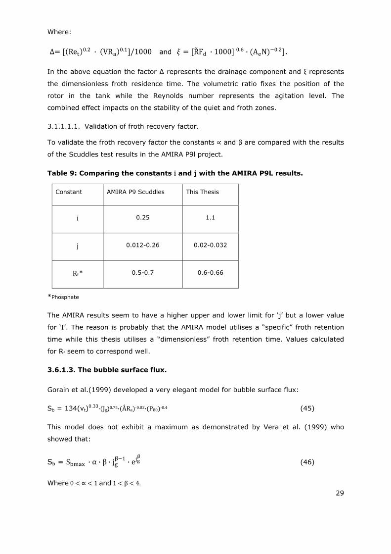
3.1.1.1.1. Validation of froth recovery factor.
To validate the froth recovery factor the constants and β are compared with the results
of the Scuddles test results in the AMIRA P9l project.
Table 9: Comparing the constants i and j with the AMIRA P9L results.
Constant AMIRA P9 Scuddles This Thesis
i 0.25 1.1
j 0.012-0.26 0.02-0.032
Rf * 0.5-0.7 0.6-0.66
*Phosphate
The AMIRA results seem to have a higher upper and lower limit for ‘j’ but a lower value
for ‘I’. The reason is probably that the AMIRA model utilises a “specific” froth retention
time while this thesis utilises a “dimensionless” froth retention time. Values calculated
for Rf seem to correspond well.
3.6.1.3. The bubble surface flux.
Gorain et al.(1999) developed a very elegant model for bubble surface flux:
Sb = 134(vt)0.33 Jg 0.75 ÅRa ‐0.02 P80 ‐0.4 (45)
This model does not exhibit a maximum as demonstrated by Vera et al. (1999) who
showed that:
Sb = S · α · β · j · e (46)
Where 0 1 and 1 β 4.
30
The first step is to rewrite Equation (46) in dimensionless form by replacing Jg with the
equivalent dimensionless number. By adding Jg to the relevant list will result in an
additional dimensionless number.
x = Jg/ω D (47)
Replacing Jg in Equation (47) with qa/D2 results in:
x = qa/ω D3 (48)
Equation (48) is the aeration number based on tank diameter and to a certain extend it
also represents the air hold-up. The next step is to find a suitable replacement for Sbmax
in Equation (46). By studying the work done by Degner and Treweek (1976) and Nelson
and Lelinsky (2000), it is evident that self aerating designs, such as the Wemco
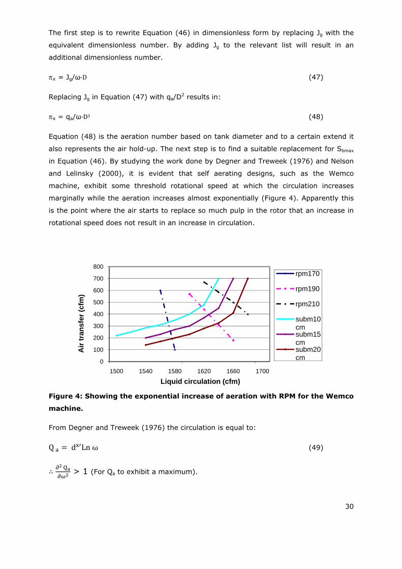
machine, exhibit some threshold rotational speed at which the circulation increases
marginally while the aeration increases almost exponentially (Figure 4). Apparently this
is the point where the air starts to replace so much pulp in the rotor that an increase in
rotational speed does not result in an increase in circulation.
Figure 4: Showing the exponential increase of aeration with RPM for the Wemco
machine.
From Degner and Treweek (1976) the circulation is equal to:
Q d Ln ω (49)
Q > 1 (For Qa to exhibit a maximum).
0
100
200
300
400
500
600
700
800
1500 1540 1580 1620 1660 1700
Air
tra
nsf
er (
cfm
)
Liquid circulation (cfm)
rpm170
rpm190
rpm210
subm10cmsubm15cmsubm20cm
31
1 (For Qa to exhibit a maximum).
From Figure 4 the critical rotational speed is equal to:
ω √ .
(50)
This is similar to the model for critical speed for rotating equipment where:
Nc = where y’’ = some maximum deflection.
Equation (51) and (52) were fitted to the Wemco information in figure 4.
q .
·ÅR
1 0.588d (51)
Where h = submergence, and:
q ·
·ÅR· d . · Ln ω (52)
where n’ = 0.85 for d < 0.76 and n’ = 0 for d > 0.76m.
From the work done by Vera et al. (1999) it seems that the maximum occurs at Jg ~ 1
cm/s. For the 1003 O/K machine in Gorain et al.’s (1999) test work at Broken Hill
concentrator with Jg=1 cm/s, requires a qa = 0.245 m3/s and with Jg = 2 requires a qa =
0.59 m3/s. From Equation (51) this will correspond with ω = 22r/s. Thus for maximum
Sb, the following variables are substituted in Equation (45):
vt = 15 m/s.
Jg = 1 or 2 cm/s.
ÅRa = 1.
P80 =75μm or 100μm.
The maximum for an external aerated machine is calculated by selecting an equivalent
self aerating machine, with the same dimensions and then determine the rotational
speed that will produce the required aeration rate according to Equation (50) and (51).
The reason for utilising Equation (45) is because it corresponds very well with measured
results according to the AMIRA P9L reports. Based on the above reasoning, the following
equation was developed for external aerated machines:
32
S 1.07x10 S Re . Ř .ŔT VR . ÅR . A N .
e A N β
(53)
For self aerating machines the equation becomes:
S 0.012 S Re Ř .
ŔT VR . ÅR. A N .
e A N (54)
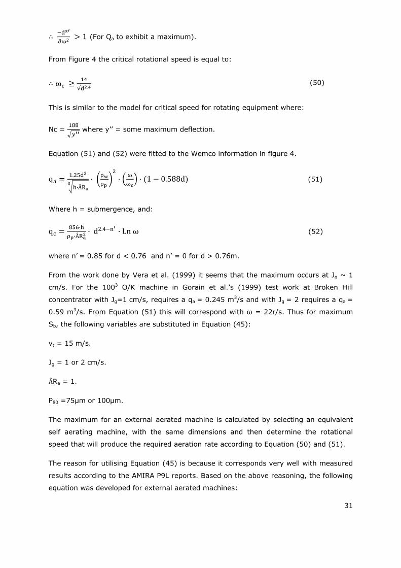
3.1.1.1.2. Validation of bubble surface area flux.
A comparison of Equation (53) and (54) with Equation (45) based on the same Pasminco
Mining Broken Hill Concentrator results, on which Gorain et al. (1999) developed the
constants and exponents for Equation (45), is given in Figure 5 & 6.
Figure 5: Bubble surface area flux as a function of aeration rate.
In Equation (53) and (54) the terms Ret VRa represent the bubble break-up mechanism,
while the other terms represent the aeration component. It is interesting to note that the
aspect ratio in Equation (45) has been replaced by the volumetric ratio and P80 by
Reynolds number. In this case the VRa can be manipulated by multiplying the VRa with
b/D which results in VRa = (D2/ÅRa h H). In the results of Gorain et al. (1999) on the
Pasminco concentrator the superficial gas velocity was measured as Jg ~ 2 cm/s and
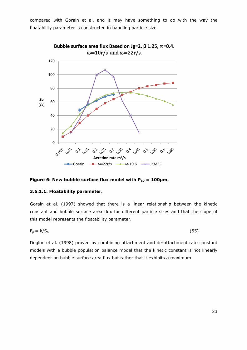
P80 = 100μm, and Figure 6 therefore is the best comparison. Figure 7 shows that the
dimensionless model predicts a lower kinetic constant at higher bubble surface area flux
0
20
40
60
80
100
120
Sb(/s)
Aeration rate (m3/s)
Bubble Surface Area Flux Based on Jg = 1 and ω = 10.6β = 1.25, = 0.35.
Gorain P80=75 P80=100 JKMRC
33
compared with Gorain et al. and it may have something to do with the way the
floatability parameter is constructed in handling particle size.
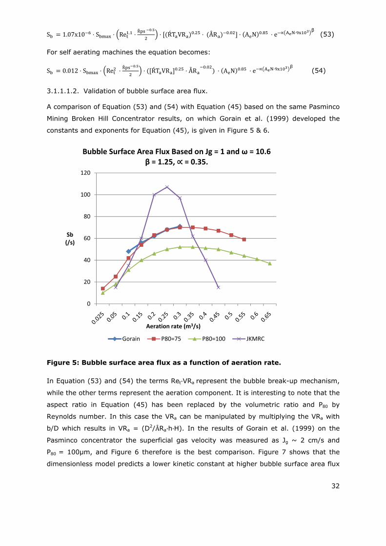
Figure 6: New bubble surface flux model with P80 = 100μm.
3.6.1.1. Floatability parameter.
Gorain et al. (1997) showed that there is a linear relationship between the kinetic
constant and bubble surface area flux for different particle sizes and that the slope of
this model represents the floatability parameter.
Fp = k/Sb (55)
Deglon et al. (1998) proved by combining attachment and de-attachment rate constant
models with a bubble population balance model that the kinetic constant is not linearly
dependent on bubble surface area flux but rather that it exhibits a maximum.
0
20
40
60
80
100
120
Sb(/s)
Aeration rate m3/s
Bubble surface area flux Based on Jg=2, β 1.25, =0.4. ω 10r/s and ω 22r/s.
Gorain ω=22r/s ω‐10.6 JKMRC

34
Figure 7: Comparison between the results obtained by Gorain and the
dimensionless model.
Deglon et al. (1998) proposed:
k
(56)
where
ka = f(є0.91) (57)
and
kd = f(є1.64) (58)
Deglon’s approach, where the kinetic constant and therefore floatability is a function of
energy dissipation rate, is more in line with the reasoning that floatability is a function of
mineral and machine properties, therefore the floatability parameter is:
Inversely dependent on particle size: The bigger the particle the more difficult it
is to suspend.
Directly dependent on circulation and Froude number: The higher the pump-
ability the better the chance of exceeding the settling velocity. Analysing the
power number resulted in a special combination of the rotor tip Reynolds number
and Froude.
‐0.05
0
0.05
0.1
0.15
0.2
0.25
0 20 40 60 80 100
Kinetic Constan
t (/m)
Bubble Surface Area Flux (/s)
Kinetic Constant vs Bubble Surface Area Flux.
Gorain model O/K Model W
35
Directly dependent on rotor tip Reynolds number or agitation.
Directly dependent on conditioning time and tank turn around: Surface
preparation.
Directly dependent on volumetric ratio: The lower the rotor in the tank the better
the ability to suspend.
Therefore:
Fp = f4 (VRa, Fr, CN, CoT, θ, Ret, Řps) . (59)
Kym Runge (AMIRA P9L report, 1999) reported in her paper on the “Conservation of
Floatability around Industrial Flotation Cells”, based on size–mineralogical-liberation
classes, that the overall circuit can also be treated as a node. In circuits where no
reagent addition and regrinding occurred, Runge stated that ore floatability was a
conserved property and did not change significantly during the residence time in the
flotation circuit. Runge, Harris and Savassi used a reverse calculation method based on
equation (1) and equation (62). By measuring variables such as bubble surface area
flux, froth depth, superficial gas velocity, particle sizes, entrainment parameters, froth
recovery factor, overall recovery, feed rates and cell dimensions, the overall kinetic
constant is estimated based on equation (1). With the kinetic constant known the
estimation of floatability parameter is based equation (62). With Barun Gorains’s results
from the Mount Isa copper process, equation (59) and through a process of trial and
error, the following model was established:
F 2 10 Řp.
VR . Re . CN Fr . η θ . . (60)
In equation (60) the tip Reynolds number represents the bubble generator while the tip
Reynolds number combined with the volumetric ratio represents the drainage factor. The
circulation number and Froude number represents solid suspension while the
conditioning parameters θ and η represents the surface preparation entrainment factor
This model seems to hold for external aerated and self aerating machines.
3.6.1.2. Validation of floatability parameter.
No specific tests have been performed to produce data of floatability but the AMIRA P9L
test results for galena and various other minerals and for different particle size and feed
rates seems to concentrate around 1x10⁻⁴ while the floatability parameter based on
dimensionless numbers according to Equation (60), for nickel and phosphate, vary
between 1x10⁻⁴ to 5x10⁻⁵.
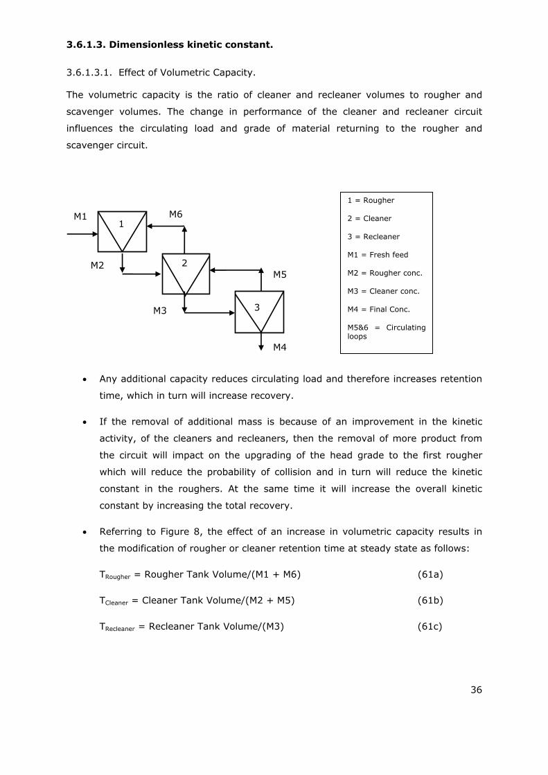
36
3.6.1.3. Dimensionless kinetic constant.
3.6.1.3.1. Effect of Volumetric Capacity.
The volumetric capacity is the ratio of cleaner and recleaner volumes to rougher and
scavenger volumes. The change in performance of the cleaner and recleaner circuit
influences the circulating load and grade of material returning to the rougher and
scavenger circuit.
Any additional capacity reduces circulating load and therefore increases retention
time, which in turn will increase recovery.
If the removal of additional mass is because of an improvement in the kinetic
activity, of the cleaners and recleaners, then the removal of more product from
the circuit will impact on the upgrading of the head grade to the first rougher
which will reduce the probability of collision and in turn will reduce the kinetic
constant in the roughers. At the same time it will increase the overall kinetic
constant by increasing the total recovery.
Referring to Figure 8, the effect of an increase in volumetric capacity results in
the modification of rougher or cleaner retention time at steady state as follows:
TRougher = Rougher Tank Volume/(M1 + M6) (61a)
TCleaner = Cleaner Tank Volume/(M2 + M5) (61b)
TRecleaner = Recleaner Tank Volume/(M3) (61c)
3
2
M1
M2
M3
M4
M5
M6 1
1 = Rougher
2 = Cleaner
3 = Recleaner
M1 = Fresh feed
M2 = Rougher conc.
M3 = Cleaner conc.
M4 = Final Conc.
M5&6 = Circulating loops
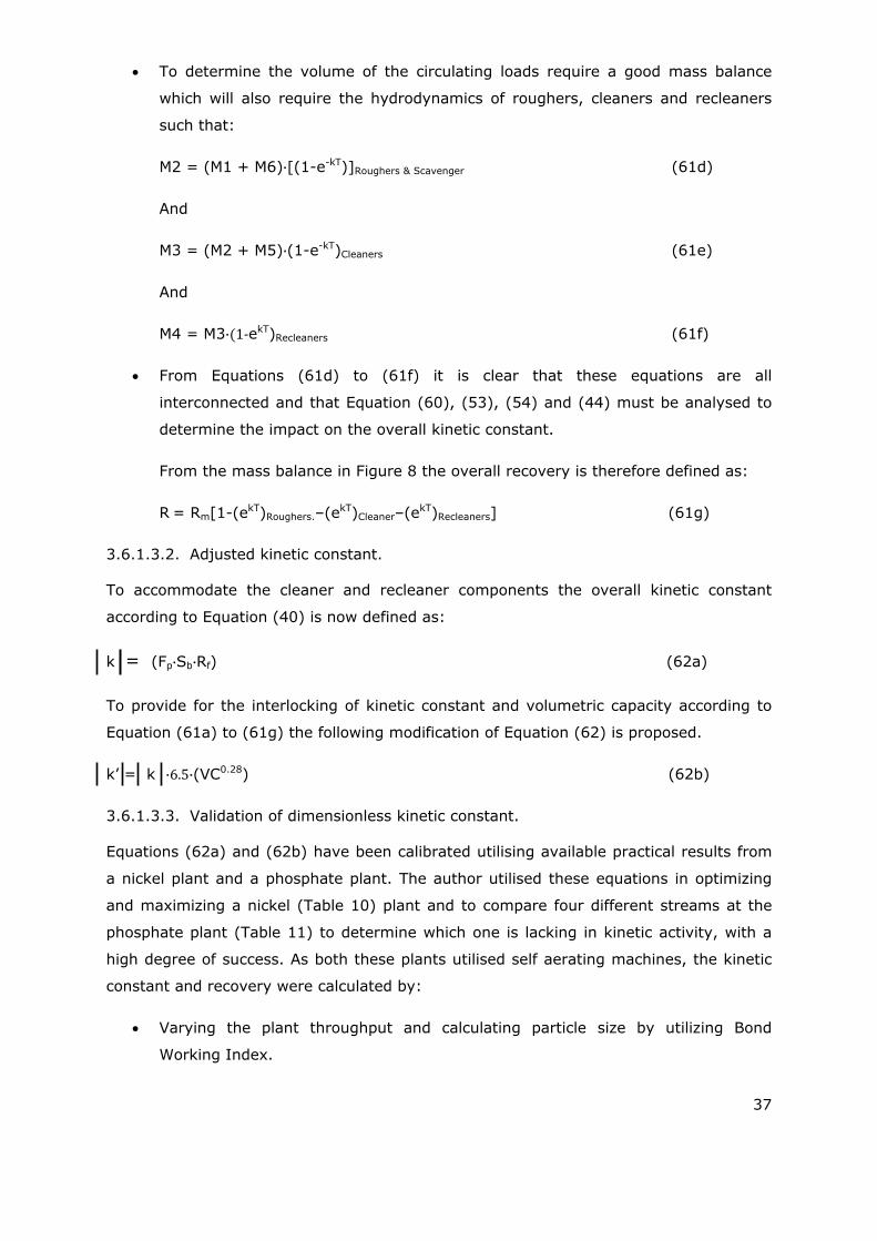
37
To determine the volume of the circulating loads require a good mass balance
which will also require the hydrodynamics of roughers, cleaners and recleaners
such that:
M2 = (M1 + M6) [(1-e-kT)]Roughers & Scavenger (61d)
And
M3 = (M2 + M5) (1-e-kT)Cleaners (61e)
And
M4 = M3 1‐ekT)Recleaners (61f)
From Equations (61d) to (61f) it is clear that these equations are all
interconnected and that Equation (60), (53), (54) and (44) must be analysed to
determine the impact on the overall kinetic constant.
From the mass balance in Figure 8 the overall recovery is therefore defined as:
R = Rm[1-(ekT)Roughers.–(ekT)Cleaner–(ekT)Recleaners] (61g)
3.6.1.3.2. Adjusted kinetic constant.
To accommodate the cleaner and recleaner components the overall kinetic constant
according to Equation (40) is now defined as:
k = (Fp Sb Rf) (62a)
To provide for the interlocking of kinetic constant and volumetric capacity according to
Equation (61a) to (61g) the following modification of Equation (62) is proposed.
k’ = k 6.5 (VC0.28) (62b)
3.6.1.3.3. Validation of dimensionless kinetic constant.
Equations (62a) and (62b) have been calibrated utilising available practical results from
a nickel plant and a phosphate plant. The author utilised these equations in optimizing
and maximizing a nickel (Table 10) plant and to compare four different streams at the
phosphate plant (Table 11) to determine which one is lacking in kinetic activity, with a
high degree of success. As both these plants utilised self aerating machines, the kinetic
constant and recovery were calculated by:
Varying the plant throughput and calculating particle size by utilizing Bond
Working Index.
38
Estimated retention time by dividing Qt/qp.
Calculate froth recovery factor, bubble surface area flux and floatability by
utilizing Equations (44), (53), 54 and (60).
Estimated k and k’ by Equation (62a) and (62b).
Estimated recovery by utilizing Equation (1).
The dimensionless floatability parameter and bubble surface area flux change with
particle size as expected. Aeration and froth depth were kept constant and therefore
the dimensionless froth recovery factor remained constant. In this experiment the
maximum nickel units coincided with 55 tph, but as a 40% loss of product was not
acceptable the plant was set at 40-45 tph.
Table 10: A comparison between measured and predicted recoveries for a
nickel plant.
Feed
tph
P80(μm)
Calculate
Sb (s-1)
Model
Fp
Model
Rf
Model
k’
min-1
τ
min
R (%)
Model
R (%)
Actual
35 130 45 9x10⁻⁴ 0.565 0.081 52 82 82
45 201 35 8.7x10⁻⁴ 0.564 0.061 42 72 73
55 282 28 8.3x10⁻⁴ 0.562 0.046 34 65 62
65 370 23 8x10⁻⁴ 0.562 0.036 26 50 49
The phosphate plant also utilised self aerating machines installed in three banks to
process three different mineral combinations. The modified E-bank was an actual
improved installation where the improvements were suggested and implemented after
analysing plant deficiencies by utilising the schedule of dimensionless numbers. The
predicted recovery was calculated by utilising Equations (44) to (60) and (62b) and (1).
Although extention-8 performed better than the original E-bank and F-bank, Table 11
shows clearly that something was drastically wrong with its kinetic activity. The
dimensionless model showed that the problem lies with aeration, bubble surface flux,
Froude number and volumetric ratio.
Equation 40-62 need to be calibrated and refined with every application as a result of
unusual modifications experienced in certain plants. Small flotation machines would be
fitted with the next size rotor modified to operate within the installed power and these
secondary changes are not covered by equations 40-62.

39
Table 11: The kinetic deficiencies between the different phosphate streams.
Plant PP E-Bank (O) Ext-8 F-bank E-Bank (M)
Feed (Tph) 0.5 600 600 1200 480
Pulp specific gravity 1.4 1.35 1.35 1.4 1.35
Rougher & Scavenger Volume (m3) 0.4 336 672 544 336
Retention time (min)* 19 12 28 10 12
Actual recovery (%) 95 72 75 55 83
Overall kinetic constant (/min) 0.35 0.16 0.055 0.09 0.18
Predicted recovery (%) 94 0.79 71 53 83
Predicted kinetic constant (/min) 0.22 0.15 0.055 0.082 0.18
(*Assumed 65% circulating load, except for pilot plant where circulating load is 50%).
3.7. Characterization of plant deficiencies based on a schedule of dimensionless numbers.
This methodology has been developed to facilitate the plant metallurgist to analyse for
deficiencies and to decide on what steps to take to improve performance based on
dimensionless numbers. A demonstration of the application of this schedule is
demonstrated in Chapters 5 & 6.
Table 12 shows the dimensionless numbers which have been selected to populate the
schedule. These numbers have been selected on the bases of practicality and in a certain
sense it is a reflection of all the variables of the kinetic constant.
3.7.1. Dimensionless parameters influencing flotation.
3.7.1.1. Dimensionless numbers and field of influence.
Table 12 shows the dimensionless groups which represents the most important and easy
measurable groups. This section describes the methods of determining the numerical
values and highlights the pitfalls and difficulties in determining these numbers.
3.7.1.2. Fundamental zones in flotation and dimensionless groups.
Mavros (1992) suggested that a flotation machine can be divided into three very distinct
zones, viz. the agitation zone, the quiet zone, and the froth zone and that each of these
zones has a very specific requirement in terms of turbulence.
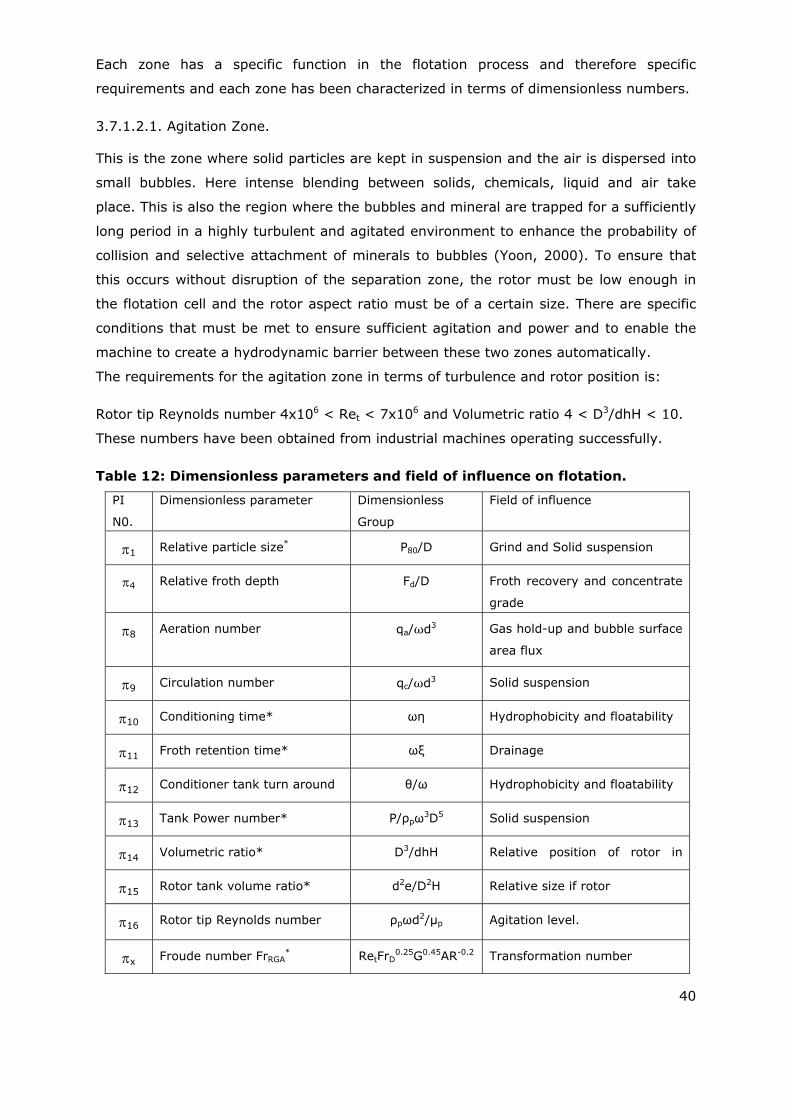
40
Each zone has a specific function in the flotation process and therefore specific
requirements and each zone has been characterized in terms of dimensionless numbers.
3.7.1.2.1. Agitation Zone.
This is the zone where solid particles are kept in suspension and the air is dispersed into
small bubbles. Here intense blending between solids, chemicals, liquid and air take
place. This is also the region where the bubbles and mineral are trapped for a sufficiently
long period in a highly turbulent and agitated environment to enhance the probability of
collision and selective attachment of minerals to bubbles (Yoon, 2000). To ensure that
this occurs without disruption of the separation zone, the rotor must be low enough in
the flotation cell and the rotor aspect ratio must be of a certain size. There are specific
conditions that must be met to ensure sufficient agitation and power and to enable the
machine to create a hydrodynamic barrier between these two zones automatically.
The requirements for the agitation zone in terms of turbulence and rotor position is:
Rotor tip Reynolds number 4x10⁶ < Ret < 7x10⁶ and Volumetric ratio 4 < D3/dhH < 10.
These numbers have been obtained from industrial machines operating successfully.
Table 12: Dimensionless parameters and field of influence on flotation.
PI
N0.
Dimensionless parameter Dimensionless
Group
Field of influence
1 Relative particle size* P80/D Grind and Solid suspension
4 Relative froth depth Fd/D Froth recovery and concentrate
grade
8 Aeration number qa/ωd3 Gas hold-up and bubble surface
area flux
9 Circulation number qc/ωd3 Solid suspension
10 Conditioning time* ωη Hydrophobicity and floatability
11 Froth retention time* ωξ Drainage
12 Conditioner tank turn around θ/ω Hydrophobicity and floatability
13 Tank Power number* P/ρpω3D5 Solid suspension
14 Volumetric ratio* D3/dhH Relative position of rotor in
k 15 Rotor tank volume ratio* d2e/D2H Relative size if rotor
16 Rotor tip Reynolds number ρpωd2/μp Agitation level.
x Froude number FrRGA* RetFrD
0.25G0.45AR-0.2 Transformation number
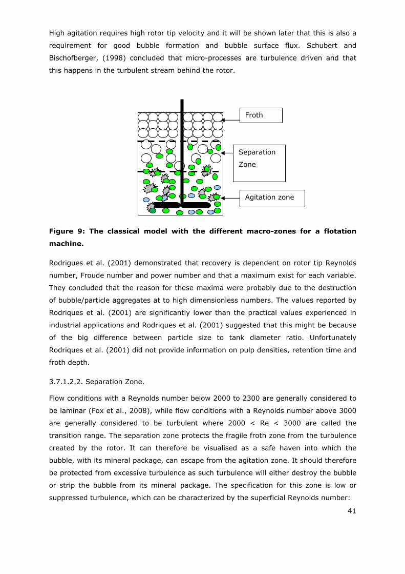
41
High agitation requires high rotor tip velocity and it will be shown later that this is also a
requirement for good bubble formation and bubble surface flux. Schubert and
Bischofberger, (1998) concluded that micro-processes are turbulence driven and that
this happens in the turbulent stream behind the rotor.
Figure 9: The classical model with the different macro-zones for a flotation
machine.
Rodrigues et al. (2001) demonstrated that recovery is dependent on rotor tip Reynolds
number, Froude number and power number and that a maximum exist for each variable.
They concluded that the reason for these maxima were probably due to the destruction
of bubble/particle aggregates at to high dimensionless numbers. The values reported by
Rodriques et al. (2001) are significantly lower than the practical values experienced in
industrial applications and Rodriques et al. (2001) suggested that this might be because
of the big difference between particle size to tank diameter ratio. Unfortunately
Rodriques et al. (2001) did not provide information on pulp densities, retention time and
froth depth.
3.7.1.2.2. Separation Zone.
Flow conditions with a Reynolds number below 2000 to 2300 are generally considered to
be laminar (Fox et al., 2008), while flow conditions with a Reynolds number above 3000
are generally considered to be turbulent where 2000 < Re < 3000 are called the
transition range. The separation zone protects the fragile froth zone from the turbulence
created by the rotor. It can therefore be visualised as a safe haven into which the
bubble, with its mineral package, can escape from the agitation zone. It should therefore
be protected from excessive turbulence as such turbulence will either destroy the bubble
or strip the bubble from its mineral package. The specification for this zone is low or
suppressed turbulence, which can be characterized by the superficial Reynolds number:
Froth
Separation
Zone
Agitation zone

42
Res = pJpD/p < 100000 (63)
The turbulence level in the separation zone is determined by two factors, namely the
rotor speed and the position of the rotor in the cell. The superficial Reynolds number is
determined by the superficial flow through the tank and is best visualised by removing
the mechanism (rotor & stator assembly) from the cell.
The value of Res < 100000 has been determined by CFD analysis and practical
investigation of industrial machines and it seems to represent a good economical level of
turbulence. Pilot plants normally operate in the laminar range (Res < 2000), but full
scale cells, which have been tested and found to perform well, operated at a superficial
Reynolds number equal to Res = 100000.
By studying the mixing theory of continuous stirred tank reactors, Wittrup (2007)
showed that the number of tanks in series required to approach the RTD of an impulse
is:
(64)
Where τ is the average residence time and ψ is the variance of the distribution function
E(t) where:
E(T) = / The probability that a certain element will still be in the tank at time t.
The variance is:
(65)
From Equation (64) it is clear that n is a dimensionless number and therefore Equation
(62) can be transformed into a dimensionless number:
n Re µ TPH. (66)
Equation (66) shows that the number of tanks in series can be expressed as a function
of superficial Reynolds number. This indicates that the superficial Reynolds number can
be used to determine the number of parallel units in a bank. As indicated in Figure 10,
the value of the superficial velocity is determined by:
Jp = qp/D H (67)
It is generally accepted that there will be some sort of velocity profile through the tank
and that this number represents a superficial horizontal velocity. In the case of so-called
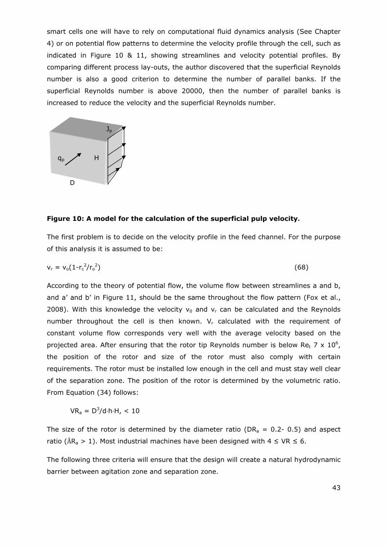
43
smart cells one will have to rely on computational fluid dynamics analysis (See Chapter
4) or on potential flow patterns to determine the velocity profile through the cell, such as
indicated in Figure 10 & 11, showing streamlines and velocity potential profiles. By
comparing different process lay-outs, the author discovered that the superficial Reynolds
number is also a good criterion to determine the number of parallel banks. If the
superficial Reynolds number is above 20000, then the number of parallel banks is
increased to reduce the velocity and the superficial Reynolds number.
Figure 10: A model for the calculation of the superficial pulp velocity.
The first problem is to decide on the velocity profile in the feed channel. For the purpose
of this analysis it is assumed to be:
vr = vo(1-rc2/ro
2) (68)
According to the theory of potential flow, the volume flow between streamlines a and b,
and a’ and b’ in Figure 11, should be the same throughout the flow pattern (Fox et al.,
2008). With this knowledge the velocity v0 and vr can be calculated and the Reynolds
number throughout the cell is then known. Vr calculated with the requirement of
constant volume flow corresponds very well with the average velocity based on the
projected area. After ensuring that the rotor tip Reynolds number is below Ret 7 x 10⁶,
the position of the rotor and size of the rotor must also comply with certain
requirements. The rotor must be installed low enough in the cell and must stay well clear
of the separation zone. The position of the rotor is determined by the volumetric ratio.
From Equation (34) follows:
VRa = D3/d h H, < 10
The size of the rotor is determined by the diameter ratio (DRa = 0.2- 0.5) and aspect
ratio (ÅRa > 1). Most industrial machines have been designed with 4 ≤ VR ≤ 6.
The following three criteria will ensure that the design will create a natural hydrodynamic
barrier between agitation zone and separation zone.
H
D
Jp
qp
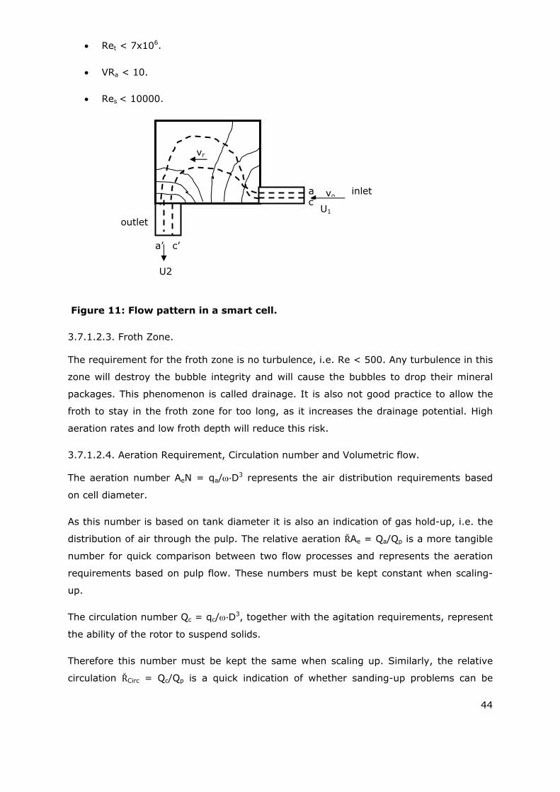
44
Ret < 7x10⁶.
VRa < 10.
Res < 10000.
Figure 11: Flow pattern in a smart cell.
3.7.1.2.3. Froth Zone.
The requirement for the froth zone is no turbulence, i.e. Re < 500. Any turbulence in this
zone will destroy the bubble integrity and will cause the bubbles to drop their mineral
packages. This phenomenon is called drainage. It is also not good practice to allow the
froth to stay in the froth zone for too long, as it increases the drainage potential. High
aeration rates and low froth depth will reduce this risk.
3.7.1.2.4. Aeration Requirement, Circulation number and Volumetric flow.
The aeration number AeN = qa/ D3 represents the air distribution requirements based
on cell diameter.
As this number is based on tank diameter it is also an indication of gas hold-up, i.e. the
distribution of air through the pulp. The relative aeration ŘAe = Qa/Qp is a more tangible
number for quick comparison between two flow processes and represents the aeration
requirements based on pulp flow. These numbers must be kept constant when scaling-
up.
The circulation number Qc = qc/ D3, together with the agitation requirements, represent
the ability of the rotor to suspend solids.
Therefore this number must be kept the same when scaling up. Similarly, the relative
circulation ŘCirc = Qc/Qp is a quick indication of whether sanding-up problems can be
a’
a
cb
c’
inlet
outlet
vo
vr
U1
U2
45
expected. Tank Turn Around (the number of times the mechanism can turn the tank
volume around in one minute) is also a valuable number for quick reference. The
volumetric flow Qp = qp/.D3 is a good indication of whether the cell or bank is
overloaded and represents to a certain extent a dimensionless retention time.
3.7.1.2.5. Froude number.
The Froude number is the primary dimensionless group when considering “partially
submerged objects”. Some researchers (Zlokarnic, 1991) have shown that the gas hold-
up in columns is a function of the Froude number. This is a bit contentious as there are
no partially submerged objects present in a flotation unit. Although air bubbles and
particles are present, they are all totally submerged. With the presence of gravity in the
Froude number, solid suspension might be a function of the Froude number and this in
turn might influence the gas hold-up capabilities in the flotation unit. Rodrigues et al.
(2001) have demonstrated with glass and quartz particles, that recovery is a function of
the Froude number and in fact that a maximum recovery exists.
3.7.1.2.6. Rotor Power Number and Tank power number.
Discussions with project managers and plant metallurgists and a study of a number of
pilot plant reports indicated that they rely on specific power consumption as an indication
of the energy requirement for a cell, but the power number indicates that there is not a
cubic relationship between cell diameter and energy requirement. After one has decided
on the pulp density for best conditioning, and d for best aeration, circulation and
agitation, then the power scale-up becomes a simple numeric calculation by keeping the
power number constant. It is interesting to compare power requirements, calculated with
the tank power number, with that calculated from kW/m3. Rodrigues et al. (2001) have
found that recovery is dependent on the power number and that a maximum recovery
exists.
Deglon et al. (1999) have proved that a maximum relationship exists between power
intensity, expressed as kW/kg, and the flotation kinetic constant, and that this maximum
appears at reduced intensity with increased tank size.
3.6.1.3.4. Summary of requirements for each zone based on practical experience.
To ensure that the machine will be able to create the required macro environment, then
the following practical specifications should be adhered to:
Geometrical requirements.
Rotor tank volume ratio; ŔTaVRa= 1.2%.
Volumetric ratio: VRa = <10.
46
Kinematic requirements.
Rotor tip Reynolds number: 4x10⁶ < Ret < 7x10⁶.
Superficial Reynolds number: Res < 100000.
Circulation number: Qc = 4.2x10⁻⁴.
Aeration number: Qa = 4.2x10⁻⁴.
Dynamic requirements.
Tank power number: 4x10⁻⁵ < TaPNo < 5x10⁻⁵.
These stated numbers have been derived from successful flotation plants in the South-
African Industry and do not vary significantly with mineral type.
3.8. Partial similarity.
Several ‘rule of thumb’ techniques exist for dimensioning different type of parameters
and are in fact scale-up rules based on partial similarity (Zlokarnic, 1991). These rules
include the so-called volume related mixing power (kW/m3) widely used for dimensioning
mixing vessels. Another partial rule for solid suspension is tank turn around per time
unit.
This is a very useful number when sizing conditioners and other mixing vessels. The
energy dissipation parameter (kW/kg) is covered by the dimensionless Froude number
and Weber number.
Newel and Grano, (2006), concluded that the energy dissipation rate is independent of
cell diameter and a function of the impeller diameter. Energy dissipation is a requirement
and not an ability, and is therefore a function of tank diameter, such that Equation (69)
is a dimensionless number.
· (69)
3.8.1. Surface tension of the pulp.
Most of the metallurgists on the plant do not have the ability or tools to determine
surface tension and hence to determine the Weber number. According to Schubert and
Bischofberger (1998), the capillary pressure over an air bubble is ∂p = 4σ/db. Where db
= bubble diameter and σ = surface tension. Substituting this in the Weber number,
gives:

47
We ·
·D . (70)
This equation proves that it is possible to reduce dimensionless numbers such as the
Weber number to simpler variables, such as a modified Froude number which is easier to
measure in practice.
3.8.2. Viscosity of the pulp.
This is probably one of the most difficult variables to determine. Although the Roscoe
model (Roscoe, 1952) is widely used, it is not clear whether this model includes the
effect of reagents and it was therefore decided to produce a viscometer from a hand held
drill modified as shown in Appendix 6. The current drawn is related to the torque which
in turn depends on the viscosity of the fluid. Very good correlation with Roscoe’s method
was found between in the range of pulp densities found in flotation.
3.9. Practical plant measurements.
To ensure some level of consistency the author tried to indicate in the following sections
where this information could be found and how to analyse and evaluate this information.
The author did not try to involve statistics but rather come up with a generic solution for
every variable. Information on conditioning, retention time and froth depth are
demonstrated graphically and pit falls are highlighted where possible. To complete the
range of information, flow diagrams are also shown as various types are encountered in
practice. Although flow diagrams are not dimensionless items it is also required that they
should stay the same between pilot plant and full scale plant, as is required for
mineralogy and reagent dosage. It is imperative to start any flotation process by
studying the mineralogy as it indicates problem minerals and secondary minerals of
value that must be stockpiles separately and this might put extra requirements on the
design of the plant. Pre-extraction of these secondary minerals might benefit the
flotation process by increasing the head grade and under certain conditions reduce and
simplifies the reagent suite and consumption.
3.9.1. Mineralogy.
3.9.1.1. Phosphate.
It is important to make sure we are dealing with the same mineral and liberation
characteristics used during the laboratory and pilot test trials.
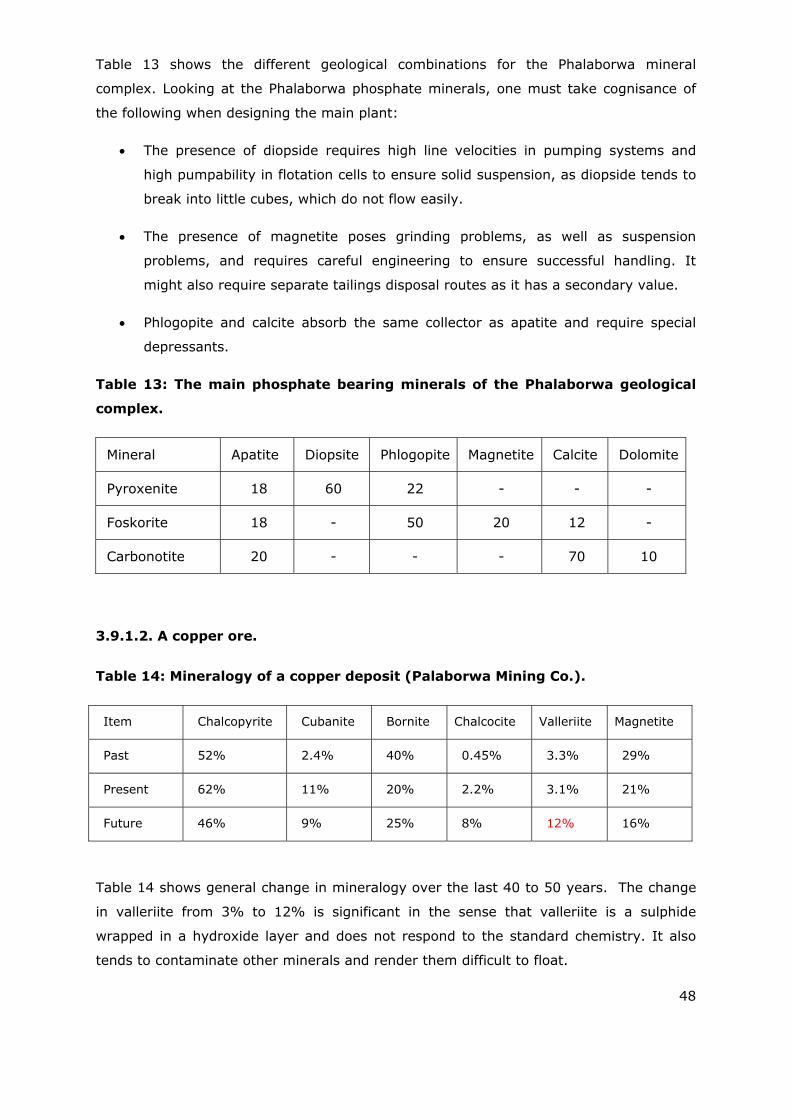
48
Table 13 shows the different geological combinations for the Phalaborwa mineral
complex. Looking at the Phalaborwa phosphate minerals, one must take cognisance of
the following when designing the main plant:
The presence of diopside requires high line velocities in pumping systems and
high pumpability in flotation cells to ensure solid suspension, as diopside tends to
break into little cubes, which do not flow easily.
The presence of magnetite poses grinding problems, as well as suspension
problems, and requires careful engineering to ensure successful handling. It
might also require separate tailings disposal routes as it has a secondary value.
Phlogopite and calcite absorb the same collector as apatite and require special
depressants.
Table 13: The main phosphate bearing minerals of the Phalaborwa geological
complex.
Mineral Apatite Diopsite Phlogopite Magnetite Calcite Dolomite
Pyroxenite 18 60 22 - - -
Foskorite 18 - 50 20 12 -
Carbonotite 20 - - - 70 10
3.9.1.2. A copper ore.
Table 14: Mineralogy of a copper deposit (Palaborwa Mining Co.).
Item Chalcopyrite Cubanite Bornite Chalcocite Valleriite Magnetite
Past 52% 2.4% 40% 0.45% 3.3% 29%
Present 62% 11% 20% 2.2% 3.1% 21%
Future 46% 9% 25% 8% 12% 16%
Table 14 shows general change in mineralogy over the last 40 to 50 years. The change
in valleriite from 3% to 12% is significant in the sense that valleriite is a sulphide
wrapped in a hydroxide layer and does not respond to the standard chemistry. It also
tends to contaminate other minerals and render them difficult to float.
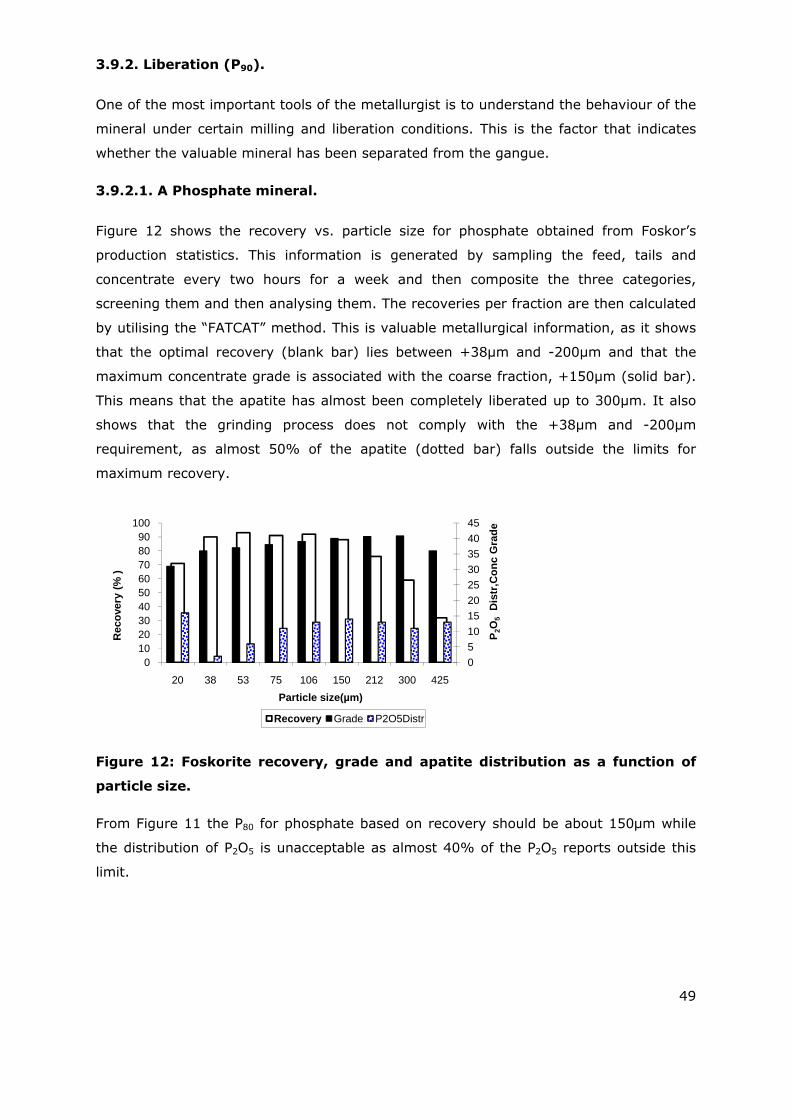
49
3.9.2. Liberation (P90).
One of the most important tools of the metallurgist is to understand the behaviour of the
mineral under certain milling and liberation conditions. This is the factor that indicates
whether the valuable mineral has been separated from the gangue.
3.9.2.1. A Phosphate mineral.
Figure 12 shows the recovery vs. particle size for phosphate obtained from Foskor’s
production statistics. This information is generated by sampling the feed, tails and
concentrate every two hours for a week and then composite the three categories,
screening them and then analysing them. The recoveries per fraction are then calculated
by utilising the “FATCAT” method. This is valuable metallurgical information, as it shows
that the optimal recovery (blank bar) lies between +38µm and -200µm and that the
maximum concentrate grade is associated with the coarse fraction, +150µm (solid bar).
This means that the apatite has almost been completely liberated up to 300µm. It also
shows that the grinding process does not comply with the +38µm and -200µm
requirement, as almost 50% of the apatite (dotted bar) falls outside the limits for
maximum recovery.
Figure 12: Foskorite recovery, grade and apatite distribution as a function of
particle size.
From Figure 11 the P80 for phosphate based on recovery should be about 150μm while
the distribution of P2O5 is unacceptable as almost 40% of the P2O5 reports outside this
limit.
0
5
10
15
20
25
30
35
40
45
0102030405060708090
100
20 38 53 75 106 150 212 300 425
P2O
5D
istr
,Co
nc
Gra
de
Rec
ove
ry (
% )
Particle size(µm)
Recovery Grade P2O5Distr
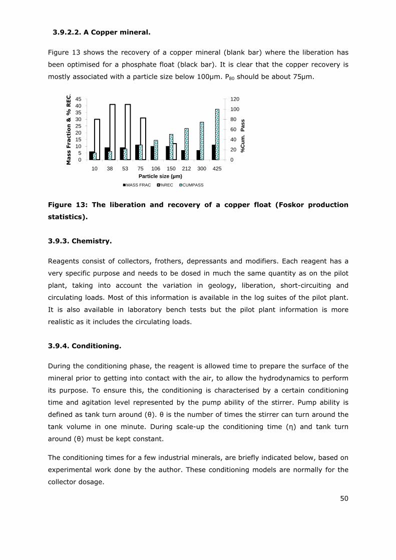
50
3.9.2.2. A Copper mineral.
Figure 13 shows the recovery of a copper mineral (blank bar) where the liberation has
been optimised for a phosphate float (black bar). It is clear that the copper recovery is
mostly associated with a particle size below 100µm. P80 should be about 75μm.
Figure 13: The liberation and recovery of a copper float (Foskor production
statistics).
3.9.3. Chemistry.
Reagents consist of collectors, frothers, depressants and modifiers. Each reagent has a
very specific purpose and needs to be dosed in much the same quantity as on the pilot
plant, taking into account the variation in geology, liberation, short-circuiting and
circulating loads. Most of this information is available in the log suites of the pilot plant.
It is also available in laboratory bench tests but the pilot plant information is more
realistic as it includes the circulating loads.
3.9.4. Conditioning.
During the conditioning phase, the reagent is allowed time to prepare the surface of the
mineral prior to getting into contact with the air, to allow the hydrodynamics to perform
its purpose. To ensure this, the conditioning is characterised by a certain conditioning
time and agitation level represented by the pump ability of the stirrer. Pump ability is
defined as tank turn around (θ). θ is the number of times the stirrer can turn around the
tank volume in one minute. During scale-up the conditioning time (η) and tank turn
around (θ) must be kept constant.
The conditioning times for a few industrial minerals, are briefly indicated below, based on
experimental work done by the author. These conditioning models are normally for the
collector dosage.
0
20
40
60
80
100
120
05
1015202530354045
10 38 53 75 106 150 212 300 425
%C
um
. P
ass
Mass
Fra
ctio
n &
% R
EC
.
Particle size (µm)
MASS FRAC %REC CUMPASS

51
3.9.4.1. Phosphate.
Figure 14 shows the behaviour for a phosphate mineral. The conditioning time in this
case should be about η = 8 minutes for a recovery of more than 80%. This should be
combined with a conditioner tank turn around θ = 9min-1. For fine grinned P80 < 100ηm,
θ should be about 7min-1.
Figure 14: Effect of conditioning time on the recovery of a phosphate mineral.
The design of the conditioner must be such that the discharge from the conditioner is at
the top of the conditioner. When no sanding up occurs then the value of θ should be
acceptable. Theta should be increased stepwise until no sand up occurs. This would
prevent theta to be too high. (See paragraph 3.9.6 for more detail). Accept for the
stirrer at the bottom, good conditioner design includes a small impeller at the top where
it creates a little vortex which is the dosage point. With such a design the reagents are
sucked into the stirrer circulating zones.
3.9.4.2. Conditioning model for a copper mineral.
Figure 15 shows the conditioning time for the Palabora copper mineralogy. Palabora
mine does not condition, although the model clearly shows about a five minutes
conditioning is required for a recovery of more than 90% (η = 5min). The rationale
behind the decision not to condition is unknown and has probably something to do with
cost during the initial design stage. This model shows that all models have similar shapes
and need careful analysis before making decisions. The irregular shape of the second
and third graphs is a result of oxidising during the preparation stage of the sample. The
tests were done over three consecutive days although all the grinding has been done on
day1.
83
0
10
20
30
40
50
60
70
80
90
1 2 3 4 5 6 7 8 9 10
Rec
ove
ry
(%)
Conditioning time (min)
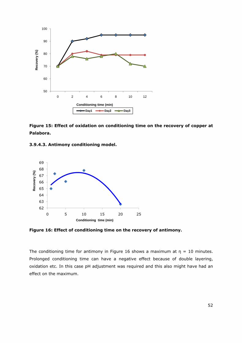
52
Figure 15: Effect of oxidation on conditioning time on the recovery of copper at
Palabora.
3.9.4.3. Antimony conditioning model.
Figure 16: Effect of conditioning time on the recovery of antimony.
The conditioning time for antimony in Figure 16 shows a maximum at η = 10 minutes.
Prolonged conditioning time can have a negative effect because of double layering,
oxidation etc. In this case pH adjustment was required and this also might have had an
effect on the maximum.
50
60
70
80
90
100
0 2 4 6 8 10 12
Rec
ove
ry(%
)
Conditioning time (min)
Day1 Day2 Day3
62
63
64
65
66
67
68
69
0 5 10 15 20 25
Rec
ove
ry (
%)
Conditioning time (min)
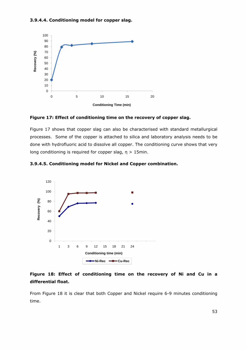
53
3.9.4.4. Conditioning model for copper slag.
Figure 17: Effect of conditioning time on the recovery of copper slag.
Figure 17 shows that copper slag can also be characterised with standard metallurgical
processes. Some of the copper is attached to silica and laboratory analysis needs to be
done with hydrofluoric acid to dissolve all copper. The conditioning curve shows that very
long conditioning is required for copper slag, η > 15min.
3.9.4.5. Conditioning model for Nickel and Copper combination.
Figure 18: Effect of conditioning time on the recovery of Ni and Cu in a
differential float.
From Figure 18 it is clear that both Copper and Nickel require 6-9 minutes conditioning
time.
0
10
20
30
40
50
60
70
80
90
100
0 5 10 15 20
Rec
ove
ry (
%)
Conditioning Time (min)
0
20
40
60
80
100
120
1 3 6 9 12 15 18 21 24
Rec
ove
ry
(%)
Conditioning time (min)
Ni-Rec Cu-Rec
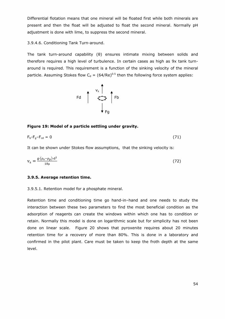
54
Differential flotation means that one mineral will be floated first while both minerals are
present and then the float will be adjusted to float the second mineral. Normally pH
adjustment is done with lime, to suppress the second mineral.
3.9.4.6. Conditioning Tank Turn-around.
The tank turn-around capability (θ) ensures intimate mixing between solids and
therefore requires a high level of turbulence. In certain cases as high as 9x tank turn-
around is required. This requirement is a function of the sinking velocity of the mineral
particle. Assuming Stokes flow Cd = (64/Re)0.5 then the following force system applies:
Figure 19: Model of a particle settling under gravity.
Fb-Fg–Fcd = 0 (71)
It can be shown under Stokes flow assumptions, that the sinking velocity is:
v· ·
µ (72)
3.9.5. Average retention time.
3.9.5.1. Retention model for a phosphate mineral.
Retention time and conditioning time go hand-in–hand and one needs to study the
interaction between these two parameters to find the most beneficial condition as the
adsorption of reagents can create the windows within which one has to condition or
retain. Normally this model is done on logarithmic scale but for simplicity has not been
done on linear scale. Figure 20 shows that pyroxenite requires about 20 minutes
retention time for a recovery of more than 80%. This is done in a laboratory and
confirmed in the pilot plant. Care must be taken to keep the froth depth at the same
level.
Fg
Fb Fd
vs

55
Figure 20: Recovery vs. retention time for pyroxenite ore.
3.9.5.2. Retention time model for Copper and Zinc.
Figure 21 shows a typical recovery vs. retention time for a copper and zinc ore. The high
recovery is a result of very high head grades and the lower zinc recovery is due to the
suppression of zinc as part of the differential flotation requirements. Retention time of
18 minutes for both copper and zinc are required
Figure 21: Recovery vs. retention time for copper and zinc.
0
10
20
30
40
50
60
70
80
90
100
1 6 12 20 30 50
Rec
ove
ry
(%)
Time (min)
0
20
40
60
80
100
120
0 4 8 12 16 18 20
%R
eco
very
Retention Time (minutes)
Cu-Rec Zn-Rec
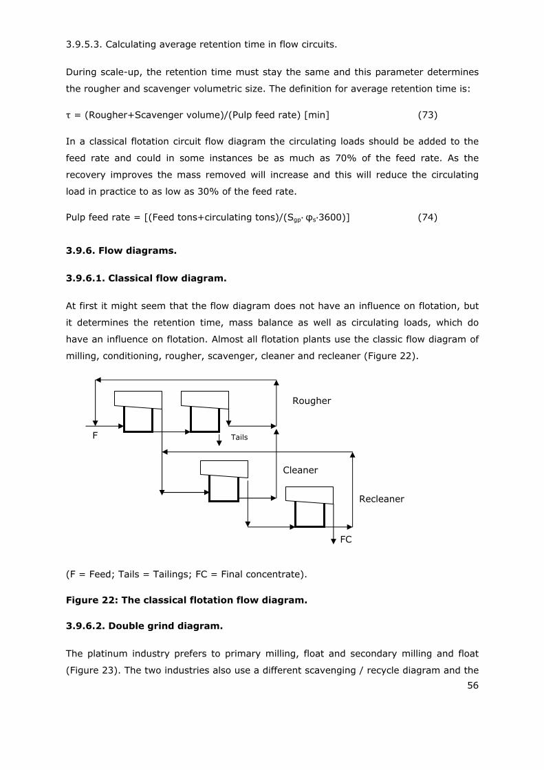
56
3.9.5.3. Calculating average retention time in flow circuits.
During scale-up, the retention time must stay the same and this parameter determines
the rougher and scavenger volumetric size. The definition for average retention time is:
τ = (Rougher+Scavenger volume)/(Pulp feed rate) [min] (73)
In a classical flotation circuit flow diagram the circulating loads should be added to the
feed rate and could in some instances be as much as 70% of the feed rate. As the
recovery improves the mass removed will increase and this will reduce the circulating
load in practice to as low as 30% of the feed rate.
Pulp feed rate = [(Feed tons+circulating tons)/(Sgp φs 3600)] (74)
3.9.6. Flow diagrams.
3.9.6.1. Classical flow diagram.
At first it might seem that the flow diagram does not have an influence on flotation, but
it determines the retention time, mass balance as well as circulating loads, which do
have an influence on flotation. Almost all flotation plants use the classic flow diagram of
milling, conditioning, rougher, scavenger, cleaner and recleaner (Figure 22).
(F = Feed; Tails = Tailings; FC = Final concentrate).
Figure 22: The classical flotation flow diagram.
3.9.6.2. Double grind diagram.
The platinum industry prefers to primary milling, float and secondary milling and float
(Figure 23). The two industries also use a different scavenging / recycle diagram and the
F
FC
Rougher
Cleaner
Recleaner
Tails
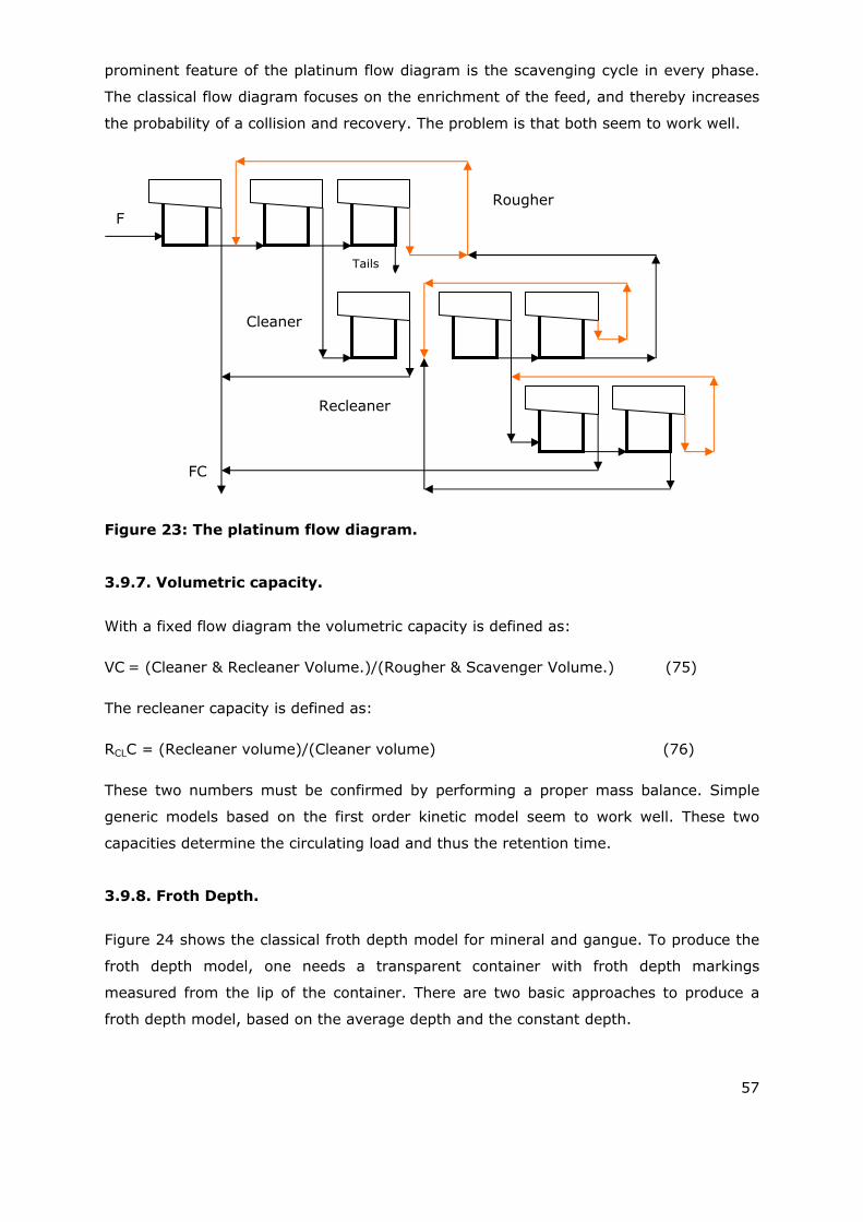
57
prominent feature of the platinum flow diagram is the scavenging cycle in every phase.
The classical flow diagram focuses on the enrichment of the feed, and thereby increases
the probability of a collision and recovery. The problem is that both seem to work well.
Figure 23: The platinum flow diagram.
3.9.7. Volumetric capacity.
With a fixed flow diagram the volumetric capacity is defined as:
VC = (Cleaner & Recleaner Volume.)/(Rougher & Scavenger Volume.) (75)
The recleaner capacity is defined as:
RCLC = (Recleaner volume)/(Cleaner volume) (76)
These two numbers must be confirmed by performing a proper mass balance. Simple
generic models based on the first order kinetic model seem to work well. These two
capacities determine the circulating load and thus the retention time.
3.9.8. Froth Depth.
Figure 24 shows the classical froth depth model for mineral and gangue. To produce the
froth depth model, one needs a transparent container with froth depth markings
measured from the lip of the container. There are two basic approaches to produce a
froth depth model, based on the average depth and the constant depth.
F
FC
Rougher
Cleaner
Recleaner
Tails
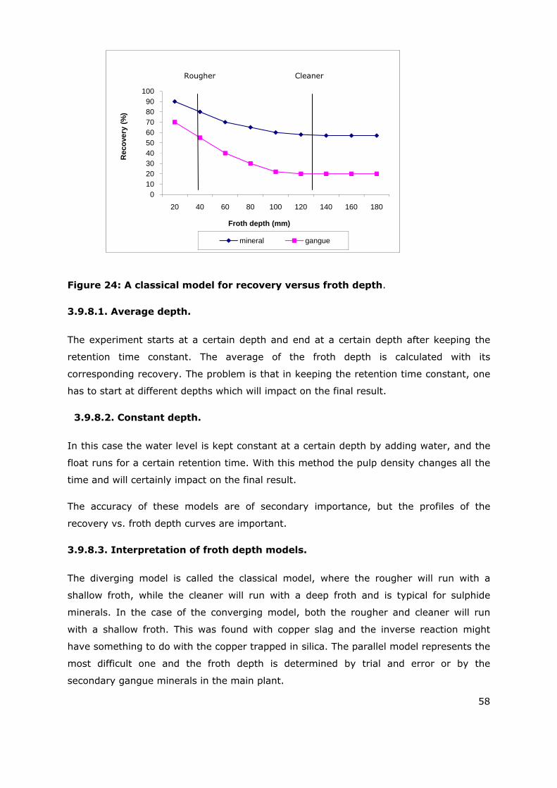
58
Figure 24: A classical model for recovery versus froth depth.
3.9.8.1. Average depth.
The experiment starts at a certain depth and end at a certain depth after keeping the
retention time constant. The average of the froth depth is calculated with its
corresponding recovery. The problem is that in keeping the retention time constant, one
has to start at different depths which will impact on the final result.
3.9.8.2. Constant depth.
In this case the water level is kept constant at a certain depth by adding water, and the
float runs for a certain retention time. With this method the pulp density changes all the
time and will certainly impact on the final result.
The accuracy of these models are of secondary importance, but the profiles of the
recovery vs. froth depth curves are important.
3.9.8.3. Interpretation of froth depth models.
The diverging model is called the classical model, where the rougher will run with a
shallow froth, while the cleaner will run with a deep froth and is typical for sulphide
minerals. In the case of the converging model, both the rougher and cleaner will run
with a shallow froth. This was found with copper slag and the inverse reaction might
have something to do with the copper trapped in silica. The parallel model represents the
most difficult one and the froth depth is determined by trial and error or by the
secondary gangue minerals in the main plant.
0102030405060708090
100
20 40 60 80 100 120 140 160 180
Rec
ove
ry (
%)
Froth depth (mm)
mineral gangue
Rougher Cleaner
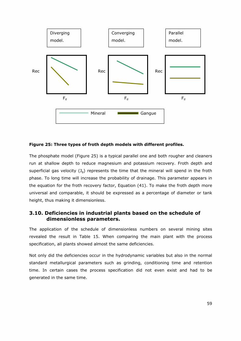
59
Figure 25: Three types of froth depth models with different profiles.
The phosphate model (Figure 25) is a typical parallel one and both rougher and cleaners
run at shallow depth to reduce magnesium and potassium recovery. Froth depth and
superficial gas velocity (Jg) represents the time that the mineral will spend in the froth
phase. To long time will increase the probability of drainage. This parameter appears in
the equation for the froth recovery factor, Equation (41). To make the froth depth more
universal and comparable, it should be expressed as a percentage of diameter or tank
height, thus making it dimensionless.
3.10. Deficiencies in industrial plants based on the schedule of dimensionless parameters.
The application of the schedule of dimensionless numbers on several mining sites
revealed the result in Table 15. When comparing the main plant with the process
specification, all plants showed almost the same deficiencies.
Not only did the deficiencies occur in the hydrodynamic variables but also in the normal
standard metallurgical parameters such as grinding, conditioning time and retention
time. In certain cases the process specification did not even exist and had to be
generated in the same time.
Rec
Fd
Rec Rec
Fd Fd
Diverging
model.
Converging
model.
Parallel
model.
Mineral Gangue

60
Table 15: Comparison of some industrial designs.
Factor Phosphate Copper Platinum Zinc Antimony Nickel
Liberation
Condition
Tank Turn Around
Retention
Flow Diagram.
Volumetric Cap.
Froth Depth
Sb
Volumetric Ratio
Res
Ret
AeN
CN
TaTu
TaPNo.
Dark= Compliance; Light= Non-compliance
In other cases operators would use aeration to control pump sump levels. Finally an
inspection of the flotation pump floor must be conducted to ensure that no pump sump
is overflowing because that is a sure indication that the recoveries recorded are not
accurate. This condition must be rectified before any measurements are taken.
These deficiencies and the non-compliance to the transformation equation based on
Froude number led to the conclusion that metallurgist, engineers and suppliers do not
understand the basic scale-up requirements. These deficiencies represent about
R7 billion revenue loss in South Africa. This represents the salaries of about 150000
employees in South Africa.
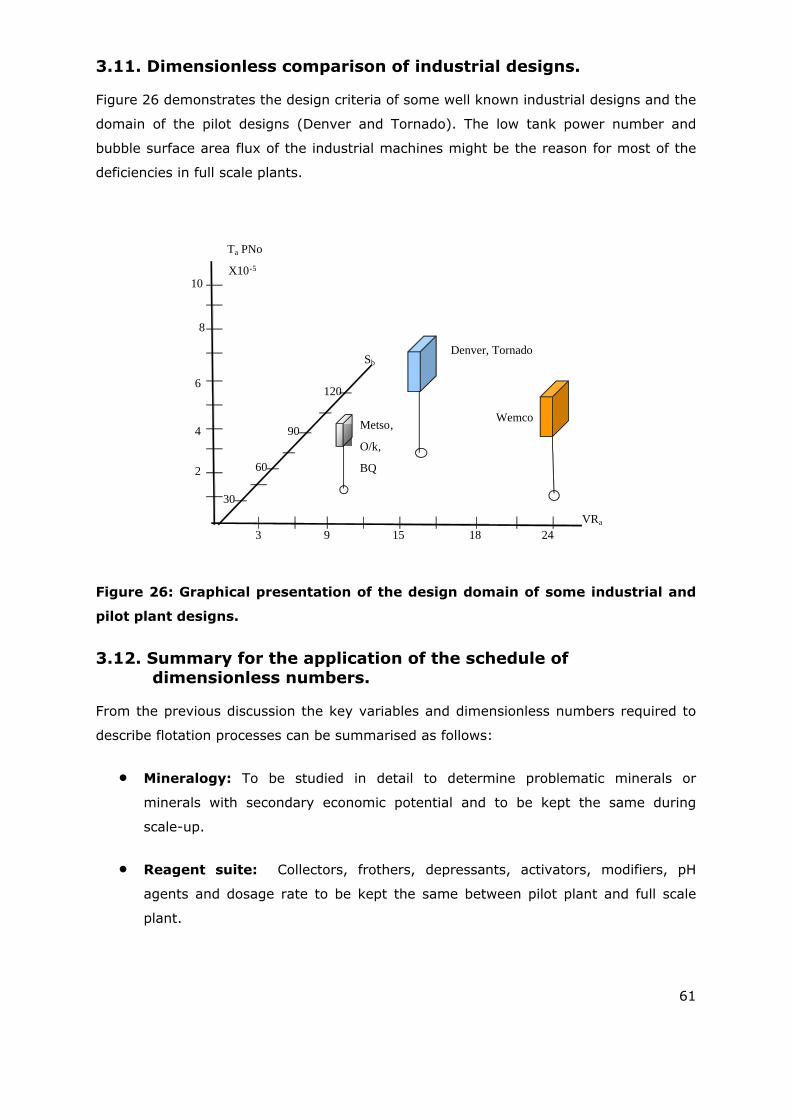
61
3.11. Dimensionless comparison of industrial designs.
Figure 26 demonstrates the design criteria of some well known industrial designs and the
domain of the pilot designs (Denver and Tornado). The low tank power number and
bubble surface area flux of the industrial machines might be the reason for most of the
deficiencies in full scale plants.
Figure 26: Graphical presentation of the design domain of some industrial and
pilot plant designs.
3.12. Summary for the application of the schedule of dimensionless numbers.
From the previous discussion the key variables and dimensionless numbers required to
describe flotation processes can be summarised as follows:
Mineralogy: To be studied in detail to determine problematic minerals or
minerals with secondary economic potential and to be kept the same during
scale-up.
Reagent suite: Collectors, frothers, depressants, activators, modifiers, pH
agents and dosage rate to be kept the same between pilot plant and full scale
plant.
3 9 15 18 24 VRa
30
60
90
120
Sb
2
4
6
8
Ta PNo
X10 - 510
Metso ,
O/k ,
BQ
Denver, Tornado
Wemco
62
Liberation: Recovery vs. particle size is a useful tool to determine milling
requirements. The characterisation process is based on laboratory scale
experiments and pilot plant results.
Conditioning: Determine conditioning time from laboratory experiments and
confirm on pilot plant. Maintain same energy input (Tank Turn Around) and
conditioning time between pilot plant and main plant.
Retention: Determine retention time on laboratory scale and confirm on pilot
plant. Combine with flow diagram configuration. Both retention time and flow
diagram to be kept the same for pilot and main plant.
Rotor tank volume ratio (d2b/D2H): Maintain same Ratio in full scale plant.
Volumetric ratio (D3/dhH): Position of rotor in tank to protect quiet and froth
zones. Maintain same ratio in full scale plant depending on basic design.
Rotor tip Reynolds number (ρpvtd/μp): Agitation level on tip of rotor. To be
combined with relative particle size ratio and to be the same for pilot plant and
main plant.
Superficial Reynolds number (ρpUD/μp): To be investigated taking
cognisance of the requirements of the mixing theory.
Rotor aspect ratio (d/b): Shape of rotor. Maintain same ratio in full scale plant
depending on basic design.
Aeration number (qa/ωD3): Required aeration. Maintain same dimensionless
number in full scale plant.
Circulation number (qc/ωD3): Solid suspension requirement. Maintain same
dimensionless number in full scale plant taking into account the multiple rotor
effect.
Froude number (ω2d2/gD): Additional requirement for solid suspension.
Combine with Ret, aspect ratio and relative particle size ratio to produce FrRGA and
maintain same dimensionless number in full scale plant.
Tank power number (P/ρpω3D5): Power requirements. Maintain same
dimensionless numbers in full scale plant.
63
Mechanism power number (P/ρpω3d5): Mechanism size. Maintain scale-up
ratio taking into account the multiple rotor effect.
Finally, a complete set of parameters are combined, in a process specification sheet
(Schedule of dimensionless numbers) to assist in the identification of plant design
deficiencies.
Although the main aim is to maintain the same dimensionless ratios in the full scale
plant design, Deglon et al. (2000) and Zlokarnic (1975) have shown that present-day
industrial designs do not comply with these objectives and varies over a large range in
almost every respect.
The next Chapter presents the results of a computational fluid dynamics analysis which
was done to get a better understanding of the hydrodynamic parameters, such as
circulation, aeration, eddies and turbulent levels in a Wemco flotation machine. The
reason for choosing the Wemco machine is that it does not represent the standard
design approach, as its volumetric ratio is very large and being a self-aerating machine,
with a low aspect ratio rotor, it requires special physical barriers to protect the
separation and froth zone.
In the following Chapter the CFD analysis presented a unique opportunity to study the
effects of these barriers and design contradictions. The dimensionless parameters such
as aeration number, AeN = qa/ωD3, rotor tip Reynolds number, Ret = ρpωd2/µp and
velocity profiles will be of particular interest.
64
CHAPTER 4: INTERPRATIVE RESULTS OF A COMPUTATIONAL FLUID DYNAMIC ANALYSIS OF FLOTATION CELL HYDRODYNAMICS.
Computational fluid dynamics (CFD) has been widely used in the analysis of complex
flow and thermal problems but very little work has been done by applying this technique
to flotation processes and flotation machine design. The WEMCO flotation machine is a
self-aerating machine utilising a low aspect ratio rotor which has been positioned high up
in the flotation tank to improve aeration ability. To protect the quiet zone from the
agitation zone, certain mechanical barriers were assembled around the rotor in the
shape of dispersers and hoods which again resulted in very complex flow patterns. To
improve circulation and solid suspension the design also features a unique false
bottom/draft tube combination which further complicates flow patterns and predictability
(See Figure 29). For this reason Megchem, represented by Beyers (2002), was
contracted to perform a CFD analysis of the Wemco machine. The client was responsible
for supplying design and process data and for the interpretation of results in terms of
dimensionless parameters. CFD analysis, based on CFX software and Perspex modelling,
have been utilised to contribute towards a better understanding of these complicated
flow patterns. As it is very difficult to undertake research on a full scale plant, this
approach provided the research team with an unique opportunity to do “what if” studies
and to eliminate expensive experimental set-ups. The objective of the study was to
quantify turbulent levels, aeration levels, solids suspension and conditions which would
support a high probability off successful recovery. As similarity is based on flow
conditions where the dimensionless groups have the same numerical value, the CFD
analysis either supported the standard analytical calculations or improved the accuracy
of the numerical values.
4.1. Design data.
4.1.1. Geometry.
The present multiphase simulations were done with the cell geometry modelled with
actual perforated disperser plates and not with porous regions. An axi-symmetric
cylindrical wedge model, with included angle of 36°, is utilised. The modelled geometry
included the as-built perforated plates is shown for clarity in Figure 27.
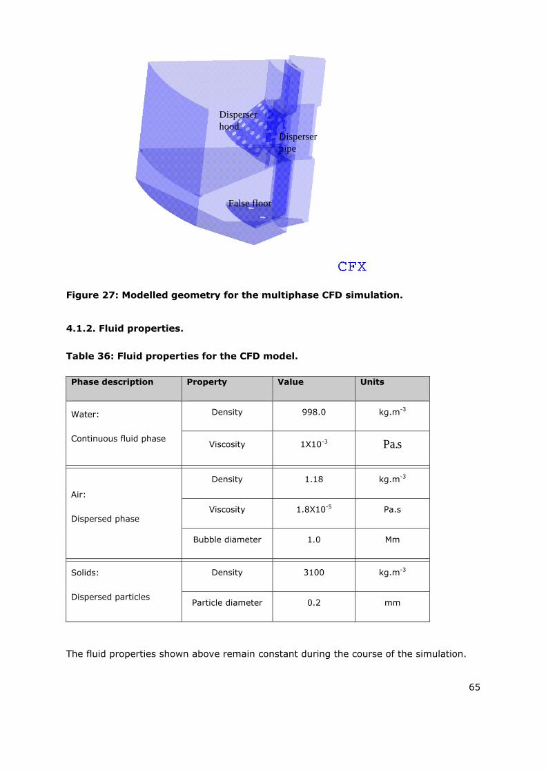
65
False floor
Disperser hood
Disperser pipe
Figure 27: Modelled geometry for the multiphase CFD simulation.
4.1.2. Fluid properties.
Table 36: Fluid properties for the CFD model.
Phase description Property Value Units
Water:
Continuous fluid phase
Density 998.0 kg.m-3
Viscosity 1X10⁻³ s.Pa
Air:
Dispersed phase
Density 1.18 kg.m-3
Viscosity 1.8X10⁻⁵ Pa.s
Bubble diameter 1.0 Mm
Solids:
Dispersed particles
Density 3100 kg.m-3
Particle diameter 0.2 mm
The fluid properties shown above remain constant during the course of the simulation.

66
4.1.3. Boundary conditions.
Boundary conditions were selected to ensure accurate physical modelling of the flotation
cell as shown in Figure 28.
Side periodic boundary
Cell wall Rotating impeller
Top pressure boundary
Top degassing boundary
Cell bottom wall
Figure 28: Boundary conditions employed.
The inlet of the stand pipe was set as a constant pressure boundary to ensure that the
induced suction generated by the impeller is not influenced by an inlet boundary but
rather implicitly calculated during the solution of the flow field. A degassing boundary
condition was assigned to the top section of the flotation cell on the outside of the stans
pipe. This type of boundary is essentially a simplified free surface that allows air to
escape through the boundary surface. Since the model consists of a 36° angle axi-
symmetric cylindrical wedge it was required to include periodic boundaries on each of the
two side planes. No other inlets or outlets were specified, thus ignoring the limited
effects of the actual inflow and outflow of the pulp. This simulation includes no inlet
mass flow boundary conditions for any of the three phases. It was established in earlier
work that the inlet boundary conditions do not greatly influence the overall flow
characteristics. It would however be beneficial to establish some inlet pulp flow condition
in the future for the axi-symmetrical wedge modelled here.
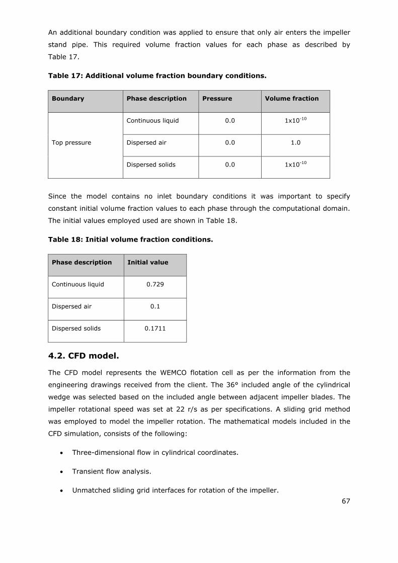
67
An additional boundary condition was applied to ensure that only air enters the impeller
stand pipe. This required volume fraction values for each phase as described by
Table 17.
Table 17: Additional volume fraction boundary conditions.
Boundary Phase description Pressure Volume fraction
Top pressure
Continuous liquid 0.0 1x10⁻¹⁰
Dispersed air 0.0 1.0
Dispersed solids 0.0 1x10⁻¹⁰
Since the model contains no inlet boundary conditions it was important to specify
constant initial volume fraction values to each phase through the computational domain.
The initial values employed used are shown in Table 18.
Table 18: Initial volume fraction conditions.
Phase description Initial value
Continuous liquid 0.729
Dispersed air 0.1
Dispersed solids 0.1711
4.2. CFD model.
The CFD model represents the WEMCO flotation cell as per the information from the
engineering drawings received from the client. The 36° included angle of the cylindrical
wedge was selected based on the included angle between adjacent impeller blades. The
impeller rotational speed was set at 22 r/s as per specifications. A sliding grid method
was employed to model the impeller rotation. The mathematical models included in the
CFD simulation, consists of the following:
Three-dimensional flow in cylindrical coordinates.
Transient flow analysis.
Unmatched sliding grid interfaces for rotation of the impeller.
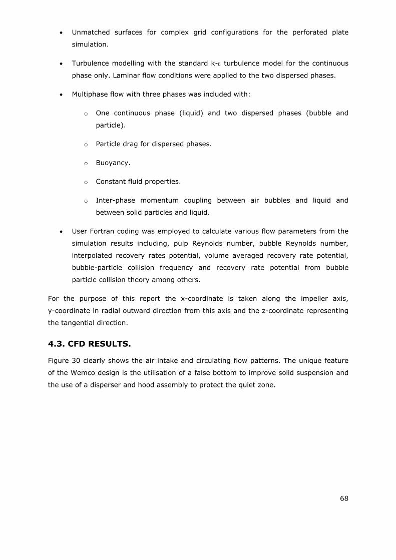
68
Unmatched surfaces for complex grid configurations for the perforated plate
simulation.
Turbulence modelling with the standard k- turbulence model for the continuous
phase only. Laminar flow conditions were applied to the two dispersed phases.
Multiphase flow with three phases was included with:
o One continuous phase (liquid) and two dispersed phases (bubble and
particle).
o Particle drag for dispersed phases.
o Buoyancy.
o Constant fluid properties.
o Inter-phase momentum coupling between air bubbles and liquid and
between solid particles and liquid.
User Fortran coding was employed to calculate various flow parameters from the
simulation results including, pulp Reynolds number, bubble Reynolds number,
interpolated recovery rates potential, volume averaged recovery rate potential,
bubble-particle collision frequency and recovery rate potential from bubble
particle collision theory among others.
For the purpose of this report the x-coordinate is taken along the impeller axis,
y-coordinate in radial outward direction from this axis and the z-coordinate representing
the tangential direction.
4.3. CFD RESULTS.
Figure 30 clearly shows the air intake and circulating flow patterns. The unique feature
of the Wemco design is the utilisation of a false bottom to improve solid suspension and
the use of a disperser and hood assembly to protect the quiet zone.
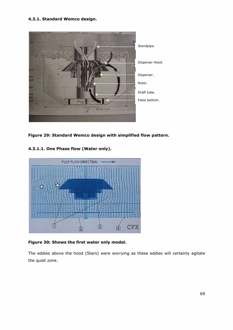
69
4.3.1. Standard Wemco design.
Figure 29: Standard Wemco design with simplified flow pattern.
4.3.1.1. One Phase flow (Water only).
Figure 30: Shows the first water only model.
The eddies above the hood (Stars) were worrying as these eddies will certainly agitate
the quiet zone.
Standpipe.
Disperser Hood.
Disperser.
Rotor.
Draft tube.
False bottom.
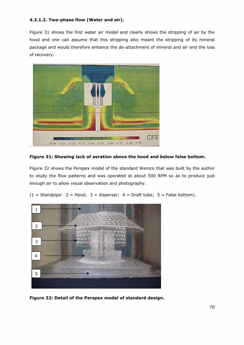
70
4.3.1.2. Two-phase flow (Water and air).
Figure 31 shows the first water air model and clearly shows the stripping of air by the
hood and one can assume that this stripping also meant the stripping of its mineral
package and would therefore enhance the de-attachment of mineral and air and the loss
of recovery.
.
Figure 31: Showing lack of aeration above the hood and below false bottom.
Figure 32 shows the Perspex model of the standard Wemco that was built by the author
to study the flow patterns and was operated at about 500 RPM so as to produce just
enough air to allow visual observation and photography.
(1 = Standpipe: 2 = Hood; 3 = disperser; 4 = Draft tube; 5 = False bottom).
Figure 32: Detail of the Perspex model of standard design.
1
2
3
4
5

71
Figure 33: Shows the Perspex model in operation.
The eddies below and above the hood (white arrows in figure 33) and also the lack of air
flow through the hood are clearly visible. The eddies and lack of air through the hood,
indicated that the CFD analysis was giving reliable results as far as flow patterns were
concerned and based on this results the three phase flow analysis (water, air and solids)
was initiated.
4.3.2. Multiphase results.
Figure 34: Streamline plot for phase 1.
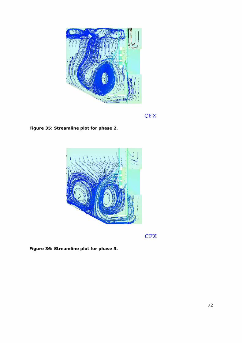
72
Figure 35: Streamline plot for phase 2.
Figure 36: Streamline plot for phase 3.
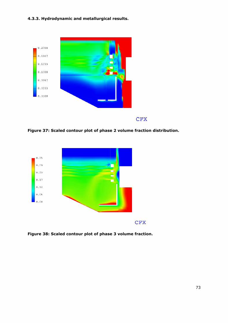
73
4.3.3. Hydrodynamic and metallurgical results.
Figure 37: Scaled contour plot of phase 2 volume fraction distribution.
Figure 38: Scaled contour plot of phase 3 volume fraction.
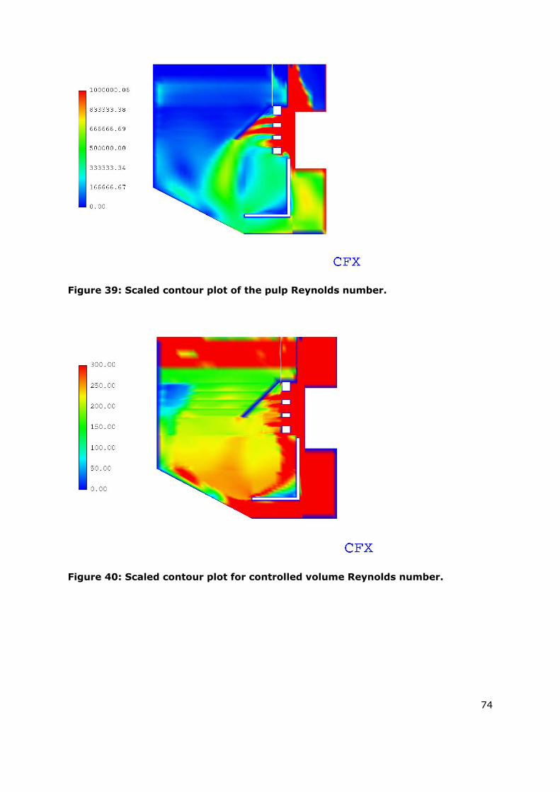
74
Figure 39: Scaled contour plot of the pulp Reynolds number.
Figure 40: Scaled contour plot for controlled volume Reynolds number.
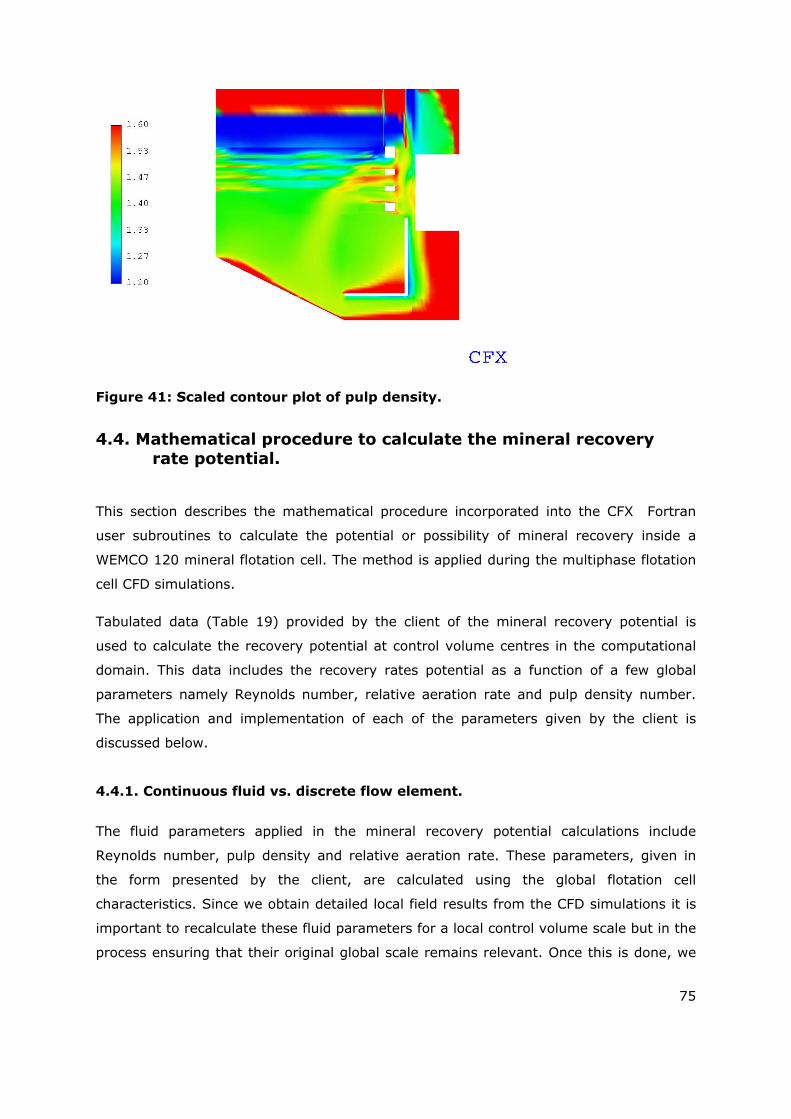
75
Figure 41: Scaled contour plot of pulp density.
4.4. Mathematical procedure to calculate the mineral recovery rate potential.
This section describes the mathematical procedure incorporated into the CFX Fortran
user subroutines to calculate the potential or possibility of mineral recovery inside a
WEMCO 120 mineral flotation cell. The method is applied during the multiphase flotation
cell CFD simulations.
Tabulated data (Table 19) provided by the client of the mineral recovery potential is
used to calculate the recovery potential at control volume centres in the computational
domain. This data includes the recovery rates potential as a function of a few global
parameters namely Reynolds number, relative aeration rate and pulp density number.
The application and implementation of each of the parameters given by the client is
discussed below.
4.4.1. Continuous fluid vs. discrete flow element.
The fluid parameters applied in the mineral recovery potential calculations include
Reynolds number, pulp density and relative aeration rate. These parameters, given in
the form presented by the client, are calculated using the global flotation cell
characteristics. Since we obtain detailed local field results from the CFD simulations it is
important to recalculate these fluid parameters for a local control volume scale but in the
process ensuring that their original global scale remains relevant. Once this is done, we
76
may assume that the fluid properties and conditions as given by the client data will
remain relevant and applicable although they are applied to the control volume scale.
4.4.2. Pulp density.
The client defines a pulp density number as:
S (77)
For calculation of fluid parameters, the local pulp density at control volume centres is
calculated for the CFD simulation from:
ρ . . (78)
The pulp density number at control volume centres then becomes:
(79)
4.4.3. Reynolds number.
The Reynolds number given and calculated by the client is based upon the impeller tip
speed, the impeller tip diameter as well as pulp density and viscosity i.e.:
. . (80)
Where the subscripts pp denotes the pulp phase and subscript t denotes the impeller tip
position. At each control volume in the CFD computational domain, the local speed and
volume fraction for each phase is available from the simulation results. For the
calculation of the local control volume Reynolds number a new Reynolds number is
defined as:
Re . .
µ (81)
Where
μcv = μf (82)
and
v V . V. (83)
77
The subscript ‘cv’ denotes control volume scale and subscript ‘f’ and ‘m’ denote
continuous fluid and mineral particle respectively. The viscosity value represented by
equation (80) should strictly speaking be the pulp viscosity but are maintained at the
initial fluid viscosity for simplicity. The new Reynolds formulation equation (81) ensures
that if fluid properties at local control volume centres are similar to flow conditions
represented by a Reynolds number based on Equation (80), then the local Reynolds
numbers calculated with equation (79) will give a similar value. Subsequently the
tabulated client data will remain relevant and applicable.
4.4.4. Relative aeration rate.
The relative aeration rate as provided by the client is based on the ratio of volume flow
rate of air at the impeller inlet draft tube to the volume flow rate of pulp in the flotation
cell i.e.:
.·A
.·A (84)
where va is the average impeller inlet air velocity and vp is the average outlet pulp
velocity. Asi denotes the impeller air standpipe diameter and Acell denotes the outlet area
for pulp flow. For the calculation of the local relative aeration rate at control volume
centres Equation (84) becomes:
.A
.A (85)
The local airflow speed is denoted by vacv and the local pulp speed denoted by vpcv = vcv.
Since Equation (85) is also based on the draft tube area and pulp outlet area similar
values will be found compared to values from Equation (84) if the air/pulp velocity ratio
is similar. Again, this ensures that the tabulated client data remains relevant and
applicable.
4.5. Interpolation of Recovery rate potential data supplied by client.
4.5.1. Interpolation method.
The mineral recovery rate potential data provided by the client is shown in Table 19. The
data given for recovery rate potentials are tabulated against specific values of pulp
density, flotation cell Reynolds number, relative aeration rate and chemical composition.
Since chemical composition is not included in the CFD simulation it was excluded from
the analysis. In order to use the recovery rate potential data at local control volume
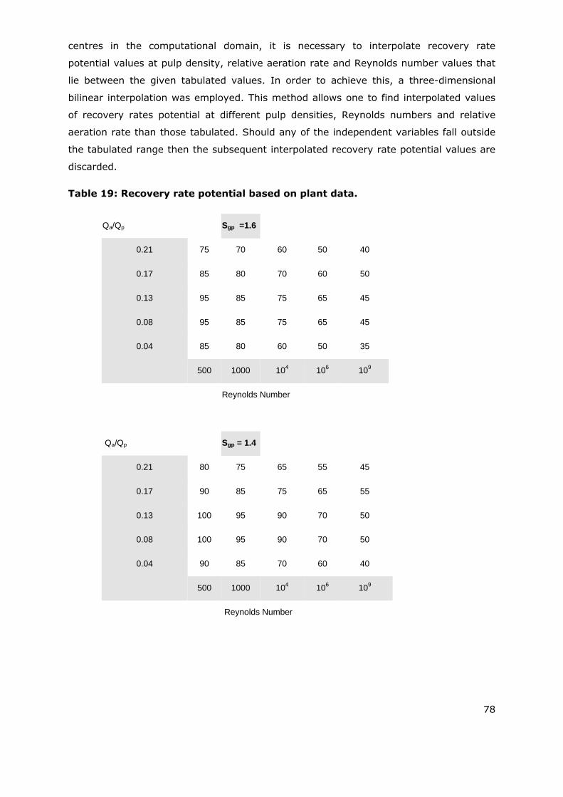
78
centres in the computational domain, it is necessary to interpolate recovery rate
potential values at pulp density, relative aeration rate and Reynolds number values that
lie between the given tabulated values. In order to achieve this, a three-dimensional
bilinear interpolation was employed. This method allows one to find interpolated values
of recovery rates potential at different pulp densities, Reynolds numbers and relative
aeration rate than those tabulated. Should any of the independent variables fall outside
the tabulated range then the subsequent interpolated recovery rate potential values are
discarded.
Table 19: Recovery rate potential based on plant data.
Qa/Qp Sgp =1.6
0.21 75 70 60 50 40
0.17 85 80 70 60 50
0.13 95 85 75 65 45
0.08 95 85 75 65 45
0.04 85 80 60 50 35
500 1000 104 106 109
Reynolds Number
Qa/Qp
Sgp = 1.4
0.21 80 75 65 55 45
0.17 90 85 75 65 55
0.13 100 95 90 70 50
0.08 100 95 90 70 50
0.04 90 85 70 60 40
500 1000 104 106 109
Reynolds Number
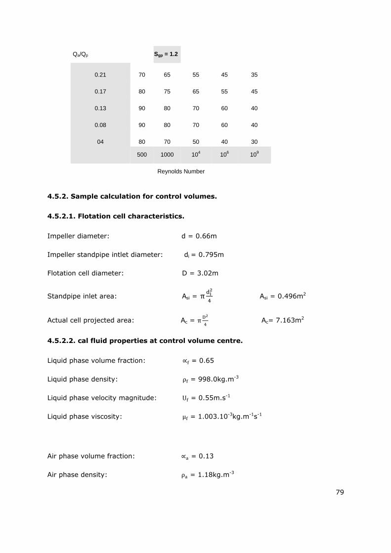
79
Qa/Qp
Sgp = 1.2
0.21 70 65 55 45 35
0.17 80 75 65 55 45
0.13 90 80 70 60 40
0.08 90 80 70 60 40
04 80 70 50 40 30
500 1000 104 106 109
Reynolds Number
4.5.2. Sample calculation for control volumes.
4.5.2.1. Flotation cell characteristics.
Impeller diameter: d = 0.66m
Impeller standpipe intlet diameter: di = 0.795m
Flotation cell diameter: D = 3.02m
Standpipe inlet area: Asi = π Asi = 0.496m2
Actual cell projected area: Ac = π D Ac= 7.163m2
4.5.2.2. cal fluid properties at control volume centre.
Liquid phase volume fraction: = 0.65
Liquid phase density: ρ = 998.0kg.m-3
Liquid phase velocity magnitude: U = 0.55m.s-1
Liquid phase viscosity: µ = 1.003.10-3kg.m-1s-1
Air phase volume fraction: = 0.13
Air phase density: ρ = 1.18kg.m-3
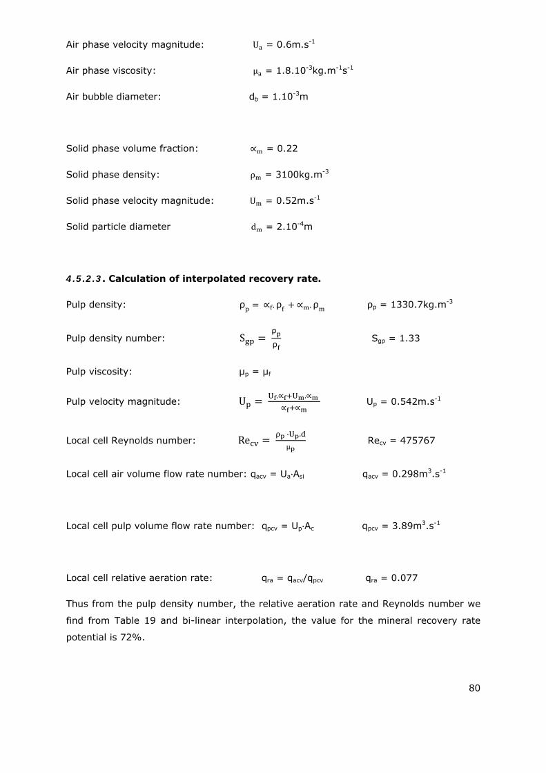
80
Air phase velocity magnitude: U = 0.6m.s-1
Air phase viscosity: µ = 1.8.10-3kg.m-1s-1
Air bubble diameter: db = 1.10-3m
Solid phase volume fraction: = 0.22
Solid phase density: ρ = 3100kg.m-3
Solid phase velocity magnitude: U = 0.52m.s-1
Solid particle diameter d = 2.10-4m
4.5.2.3. Calculation of interpolated recovery rate.
Pulp density: ρ .ρ .ρ ρp = 1330.7kg.m-3
Pulp density number: S ρ
ρ Sgp = 1.33
Pulp viscosity: μp = μf
Pulp velocity magnitude: U U . U . Up = 0.542m.s-1
Local cell Reynolds number: Re ·U .
µ Recv = 475767
Local cell air volume flow rate number: qacv = Ua Asi qacv = 0.298m3.s-1
Local cell pulp volume flow rate number: qpcv = Up Ac qpcv = 3.89m3.s-1
Local cell relative aeration rate: qra = qacv/qpcv qra = 0.077
Thus from the pulp density number, the relative aeration rate and Reynolds number we
find from Table 19 and bi-linear interpolation, the value for the mineral recovery rate
potential is 72%.
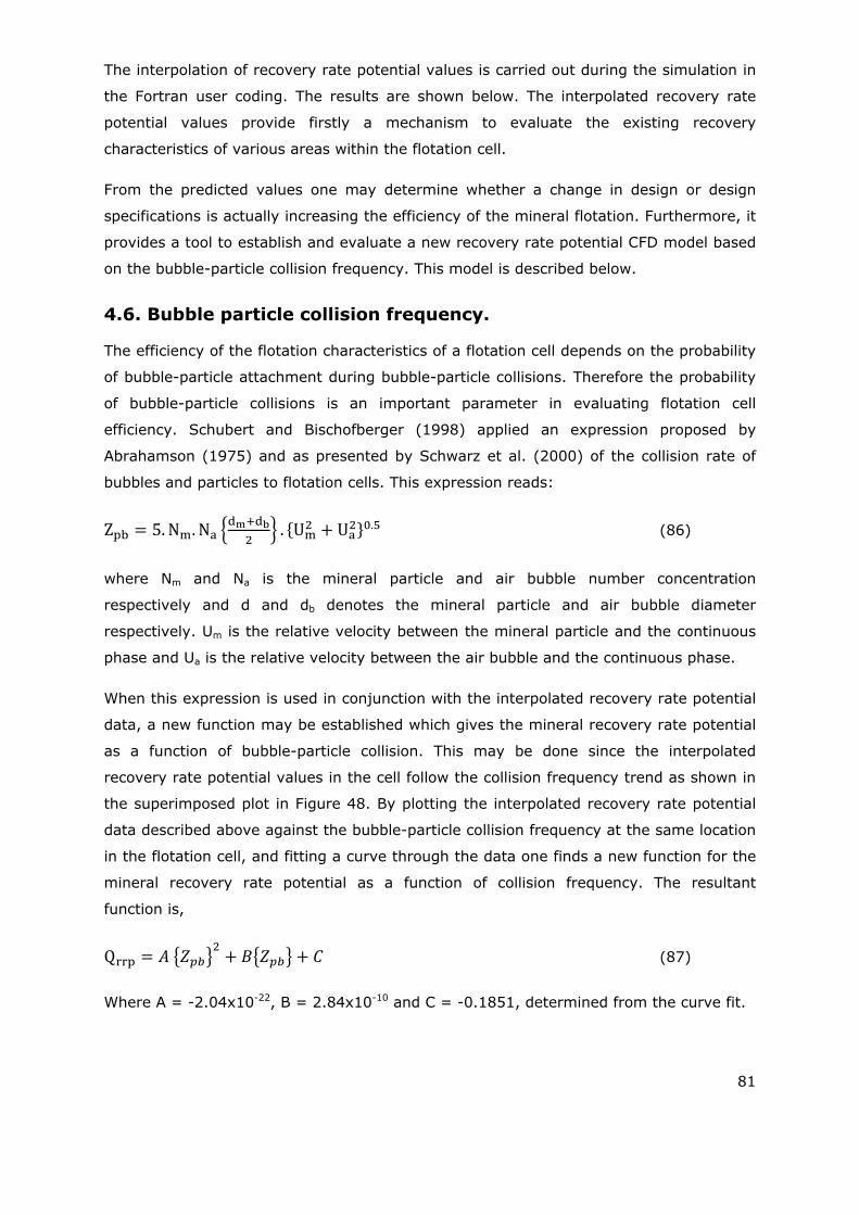
81
The interpolation of recovery rate potential values is carried out during the simulation in
the Fortran user coding. The results are shown below. The interpolated recovery rate
potential values provide firstly a mechanism to evaluate the existing recovery
characteristics of various areas within the flotation cell.
From the predicted values one may determine whether a change in design or design
specifications is actually increasing the efficiency of the mineral flotation. Furthermore, it
provides a tool to establish and evaluate a new recovery rate potential CFD model based
on the bubble-particle collision frequency. This model is described below.
4.6. Bubble particle collision frequency.
The efficiency of the flotation characteristics of a flotation cell depends on the probability
of bubble-particle attachment during bubble-particle collisions. Therefore the probability
of bubble-particle collisions is an important parameter in evaluating flotation cell
efficiency. Schubert and Bischofberger (1998) applied an expression proposed by
Abrahamson (1975) and as presented by Schwarz et al. (2000) of the collision rate of
bubbles and particles to flotation cells. This expression reads:
Z 5. N . N . U U . (86)
where Nm and Na is the mineral particle and air bubble number concentration
respectively and d and db denotes the mineral particle and air bubble diameter
respectively. Um is the relative velocity between the mineral particle and the continuous
phase and Ua is the relative velocity between the air bubble and the continuous phase.
When this expression is used in conjunction with the interpolated recovery rate potential
data, a new function may be established which gives the mineral recovery rate potential
as a function of bubble-particle collision. This may be done since the interpolated
recovery rate potential values in the cell follow the collision frequency trend as shown in
the superimposed plot in Figure 48. By plotting the interpolated recovery rate potential
data described above against the bubble-particle collision frequency at the same location
in the flotation cell, and fitting a curve through the data one finds a new function for the
mineral recovery rate potential as a function of collision frequency. The resultant
function is,
Q (87)
Where A = -2.04x10⁻²², B = 2.84x10⁻¹⁰ and C = -0.1851, determined from the curve fit.
82
4.7. Streamline plots.
Figure 34 to Figure 36 show the streamline distributions for each of the three phases.
The streamline plots clearly supports the above arguments further. The plots indicate the
circulation zones inside the flotation cell also shown by the velocity vector plots. The
liquid phase sets up two strong circulation zones arising from the channelling of the flow
downwards from the disperser hood. The solid particles are entrained in these circulation
zones. The bubbles are also circulated in the inner circulation zone closest to the impeller
bottom draft tube. The bubbles however leave the outer recirculation zone since the
buoyancy force dominates their trajectory.
4.8. Volume fraction distribution.
Figure 37 and Figure 38 show the volume fraction predictions for phases two and three.
The liquid phase is relatively equally dispersed throughout the flotation cell except at the
impeller top inlet area and the outer top surface. Air is sucked in through the top of the
impeller and leaves the flotation cell through the top de-gassing boundary. The induced
air suction of the impeller seems to be accurately simulated. The scaled distribution plot
of the air phase volume fraction indicates that the distribution of air bubbles through the
remainder of the flotation cell is of the order of 1%. Although this volume fraction seems
low, it still corresponds to approximately 19x106 bubbles per cubic metre. The solid
particles are also distributed relatively equally throughout the internal area of the
flotation cell. Since the solid particles are heavier than the liquid phase it is expected to
settle on the bottom surfaces. This is clearly shown in the scaled volume fraction plot of
the solid phase. Particles tend to concentrate on the bottom floor as well as the false
floor. Particles also concentrate near the impeller bottom shaft section.
4.9. Pulp Reynolds number.
Figure 39 shows the pulp Reynolds number plot for the flotation cell. Figure 40 shows
the control volume Reynolds number as per Equation (81). The plots show that the pulp
Reynolds numbers are high in the agitation zone and become progressively less towards
the collection zone.
4.10. Pulp density distribution.
Figure 41 show the contour plot of the relative density as defined by Equation (76).
These are shown to indicate the areas where the Foskor recovery rate data and
subsequently the interpolated recovery rate values are applicable namely
1.2 < Sgcv < 1.6.

83
4.11. Bubble particle collision frequency and probability for successful recovery.
Figure 42: Showing the contour plot for the interpolated mineral recovery
success rate.
Figure 43: Iso–surface plot for a 65% interpolated mineral recovery success
rate.
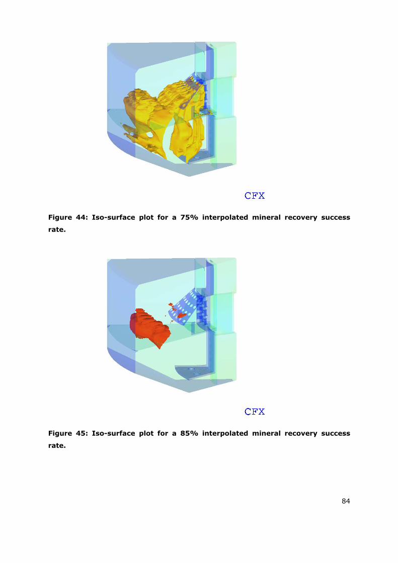
84
Figure 44: Iso-surface plot for a 75% interpolated mineral recovery success
rate.
Figure 45: Iso-surface plot for a 85% interpolated mineral recovery success
rate.
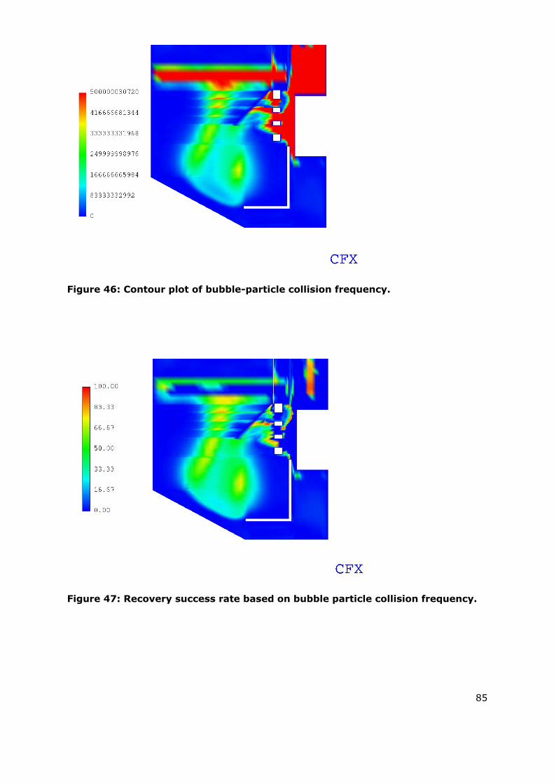
85
Figure 46: Contour plot of bubble-particle collision frequency.
Figure 47: Recovery success rate based on bubble particle collision frequency.
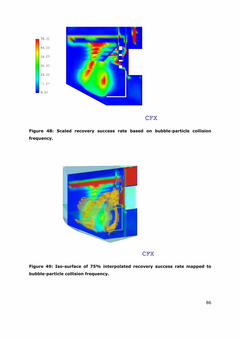
86
Figure 48: Scaled recovery success rate based on bubble-particle collision
frequency.
Figure 49: Iso-surface of 75% interpolated recovery success rate mapped to
bubble-particle collision frequency.
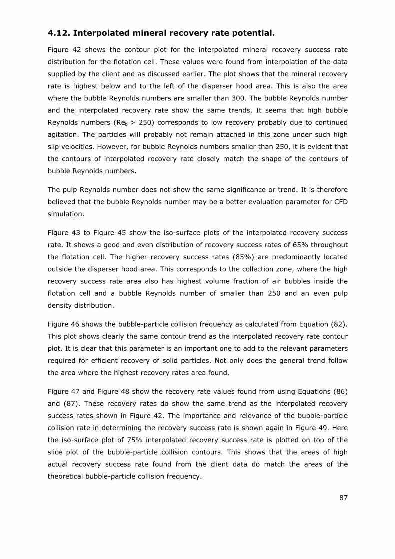
87
4.12. Interpolated mineral recovery rate potential.
Figure 42 shows the contour plot for the interpolated mineral recovery success rate
distribution for the flotation cell. These values were found from interpolation of the data
supplied by the client and as discussed earlier. The plot shows that the mineral recovery
rate is highest below and to the left of the disperser hood area. This is also the area
where the bubble Reynolds numbers are smaller than 300. The bubble Reynolds number
and the interpolated recovery rate show the same trends. It seems that high bubble
Reynolds numbers (Reb > 250) corresponds to low recovery probably due to continued
agitation. The particles will probably not remain attached in this zone under such high
slip velocities. However, for bubble Reynolds numbers smaller than 250, it is evident that
the contours of interpolated recovery rate closely match the shape of the contours of
bubble Reynolds numbers.
The pulp Reynolds number does not show the same significance or trend. It is therefore
believed that the bubble Reynolds number may be a better evaluation parameter for CFD
simulation.
Figure 43 to Figure 45 show the iso-surface plots of the interpolated recovery success
rate. It shows a good and even distribution of recovery success rates of 65% throughout
the flotation cell. The higher recovery success rates (85%) are predominantly located
outside the disperser hood area. This corresponds to the collection zone, where the high
recovery success rate area also has highest volume fraction of air bubbles inside the
flotation cell and a bubble Reynolds number of smaller than 250 and an even pulp
density distribution.
Figure 46 shows the bubble-particle collision frequency as calculated from Equation (82).
This plot shows clearly the same contour trend as the interpolated recovery rate contour
plot. It is clear that this parameter is an important one to add to the relevant parameters
required for efficient recovery of solid particles. Not only does the general trend follow
the area where the highest recovery rates area found.
Figure 47 and Figure 48 show the recovery rate values found from using Equations (86)
and (87). These recovery rates do show the same trend as the interpolated recovery
success rates shown in Figure 42. The importance and relevance of the bubble-particle
collision rate in determining the recovery success rate is shown again in Figure 49. Here
the iso-surface plot of 75% interpolated recovery success rate is plotted on top of the
slice plot of the bubble-particle collision contours. This shows that the areas of high
actual recovery success rate found from the client data do match the areas of the
theoretical bubble-particle collision frequency.
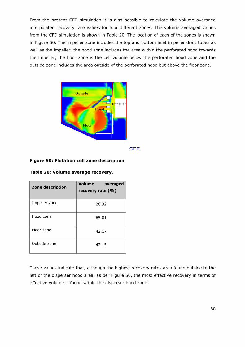
88
From the present CFD simulation it is also possible to calculate the volume averaged
interpolated recovery rate values for four different zones. The volume averaged values
from the CFD simulation is shown in Table 20. The location of each of the zones is shown
in Figure 50. The impeller zone includes the top and bottom inlet impeller draft tubes as
well as the impeller, the hood zone includes the area within the perforated hood towards
the impeller, the floor zone is the cell volume below the perforated hood zone and the
outside zone includes the area outside of the perforated hood but above the floor zone.
Floor
Outside
Hood
Im peller
Figure 50: Flotation cell zone description.
Table 20: Volume average recovery.
Zone description Volume averaged
recovery rate (%)
Impeller zone 28.32
Hood zone 65.81
Floor zone 42.17
Outside zone 42.15
These values indicate that, although the highest recovery rates area found outside to the
left of the disperser hood area, as per Figure 50, the most effective recovery in terms of
effective volume is found within the disperser hood zone.
89
4.13. Summary of CFD results.
The possibility exists that the disperser and hood in the standard Wemco design
may strip the pulp from its air and indirectly stripping it from its mineral package
too. By modifying the hood and disperser slots, plus adding a separation disc on
the rotor displaced the eddies towards the false bottom thereby improving the
conditions required for quiet zone protection. Further analysis of the recovery rate
potential also indicated a marked improvement in the 75% iso-surface.
Perspex modelling is a useful tool to study aeration, air dispersion, streamlines,
eddies and vortex stability.
Deglon et al. (2000) and Nelson and Lelinski measured and calculated the air
hold-up for the Wemco to be between 7%-12%. Figure 29 shows a 3%-17% air
hold-up which compares very favourable with the published results. Therefore the
aeration number of Qa = qa/ωd3 = idem is an acceptable scale-up number. A
aeration number of Qa = 4.6x10⁻⁴ is equal to an air hold-up of
4.6x10⁻⁴ ω Qa/D3 10.6%.
Figure 39 shows a rotor tip Reynolds number in the agitation zone to vary
between 7x10⁶ to 9x10⁶. These numbers were calculated with water density
(1000kg/m3) and viscosity (1x10⁻³kg/ms). When adjusted with a pulp density of
1300kg/m3 and a viscosity of 1.6x10⁻³kg/ms then the Reynolds numbers reduce
to 5x10⁶ to 7x10⁶ which corresponds very well with practical calculated results.
The relatively low bubble Reynolds number can have a favourable effect on
bubble particle attachment as this Reynolds number is in the laminar range.
Figure 39 also shows a very sharp dissipation of the Reynolds number, which
corresponds well with the observations done by Deglon et al. (2000) and Newel
and Grano(2007). This is substantially higher than the superficial Reynolds
number calculated. It seems that the numerical value for superficial Reynolds
number should be increased by about 50% for scale-up purposes.
The favourable comparison between the interpolated recovery rate potential and
the bubble particle collision frequency was a surprising discovery as practical
results in the plant were rearranged by swapping 100% probability of a 60%
recovery to a 60% probability of a successful recovery.
The threshold RPM in the Perspex models corresponds with the Wemco
hydrodynamic information.
90
CHAPTER5: APPLICATION OF SCHEDULE OF DIMENSIONLESS NUMBERS TO A PHOSPHATE PLANT.
5.1. Background.
The Phalaborwa complex is an igneous complex that was discovered by Dr Hans
Merensky in the 1940’s. Foskor was established shortly after this discovery in 1952. The
ore is predominantly Ca-Mg-combinations with chlorides and fluorides as problem
process components. The plant started with two 50 tons per hour rod mills and a
flotation plant equipped with 1.5m3 Denver cells. Being removed from the South African
Industrial hub the management established one of the best equipped laboratories and
pilot plants north of Pretoria. During the 1960’s the mill plant was extended to 12 x 50
tons per hour rod mills and the flotation plant was also extended to include about 150 x
1.5m3 Denver cells. In the 1970’s the mill plant was extended again to include another
12 x 100 tons per hour rod mills and the flotation plant to about 180 x 8.5 m3 Wemco
units. The plant was divided into three sections as each section processed a different ore
combination. The three types of ore are shown in Appendix 6 specification sheet 1 to 3.
The reason was that the three types of ore required three different types of reagent
suites. This pushed the throughput to about 3000 tons per hour and at 7.5% P2O5 head
grade produced 3 million tons concentrate at 37% P2O5.
The rest of the plant consisted of thickeners, filters, drying, dispatch and tailings
handling. In this case study the focus was on the pyroxenite section. From its inception
the plant operated at 75% recovery and 37% concentrate grade, while the pilot plant
performed at a 95% recovery and 40% concentrate grade with the same mineralogy.
The performance of the main plant stayed the same irrespective of ore type, machine
type and machine size. This represented about R100m/a revenue loss at that stage. In
2002 the plant was analysed according to the principles and technique described in this
thesis and the results are described in the rest if this Chapter.
In order to develop some methodology to accumulate all the relevant information, a
specification sheet was used that prompts the metallurgist to enter the information in
such a way as to facilitate the comparison of the various scale-up factors between pilot
plant and full scale plant. The specification column is normally pilot plant information. To
demonstrate how to compile the specification sheet, a phosphate mineral in a Denver
pilot plant will serve as an example.
91
5.2. Geology.
The outcrops of the Phalaborwa complex belong to rocks of the plutonic origin. No
volcanic equivalents are found, which means that great volumes of this complex have
been eroded away. This complex consists predominantly of pyroxenite (igneous) rocks,
with intruded granites and gneisses. Three prominent pipe-like features with concentric
structures flow into one another, forming lobes, named the Northern pyroxenite,
Loolekop and Southern pyroxenite. The Loolekop lobe is an old volcanic structure and
contains approximately 0.8% copper, 20% magnetite, 5% apatite, phlogopite and small
amounts of Gold, Silver and Thorium.
5.3. Pilot plant conditions.
5.3.1. Pilot plant lay-out.
The pilot plant was established to provide Foskor with the ability to develop a unique
process with unique reagents as the industrial circumstances were such that no
information was available to the Foskor at that stage and had to develop the process
from what was available in the country in 1952. Denver equipment was available and a
standard lay-out was established and configured as shown in Figure 50. Reagents were
much different then and had to be prepared on site sodium silicate, guar and the process
was also heated because of the availability of access steam as Foskor generated its own
electricity in the 1950’s and 60’s.
5.3.2. Mineralogy.
The mineralogy of this complex is shown in Appendix 6. The mineralogy is important in
the scale-up phase as it indicates the type of reagents to target and also provides
valuable information for plant pump systems and milling circuit design. In this case the
magnetite and diopside require a line-velocity of more than 3m/s to prevent settling and
also require special milling conditions. The phlogopite and Calcite compete with the
apatite for fatty acid and therefore special suppressants will have to be developed for
these minerals.
5.3.3. Operational Information and flow diagram.
5.3.3.1. Operational conditions.
The pilot plant is equipped with continuous pulp density meter and mass flow meter and
feed, tails and concentrate are sampled every hour. Analysis are done on every sample
and a composite is prepared at the end of every day and analysed by a second
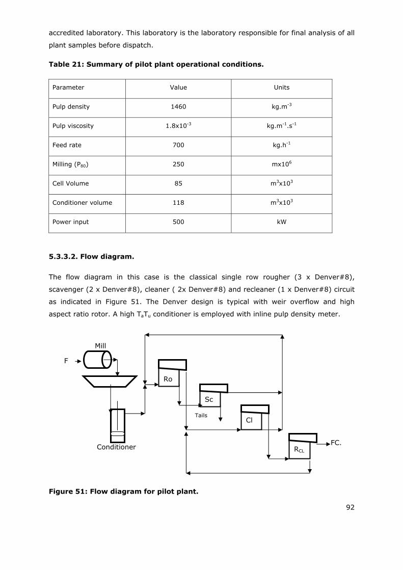
92
accredited laboratory. This laboratory is the laboratory responsible for final analysis of all
plant samples before dispatch.
Table 21: Summary of pilot plant operational conditions.
Parameter Value Units
Pulp density 1460 kg.m-3
Pulp viscosity 1.8x10⁻³ kg.m-1.s-1
Feed rate 700 kg.h-1
Milling (P80) 250 mx106
Cell Volume 85 m3x103
Conditioner volume 118 m3x103
Power input 500 kW
5.3.3.2. Flow diagram.
The flow diagram in this case is the classical single row rougher (3 x Denver#8),
scavenger (2 x Denver#8), cleaner ( 2x Denver#8) and recleaner (1 x Denver#8) circuit
as indicated in Figure 51. The Denver design is typical with weir overflow and high
aspect ratio rotor. A high TaTu conditioner is employed with inline pulp density meter.
Figure 51: Flow diagram for pilot plant.
Ro
Sc
Cl
RCL
FC.
Mill
Conditioner
F
Tails
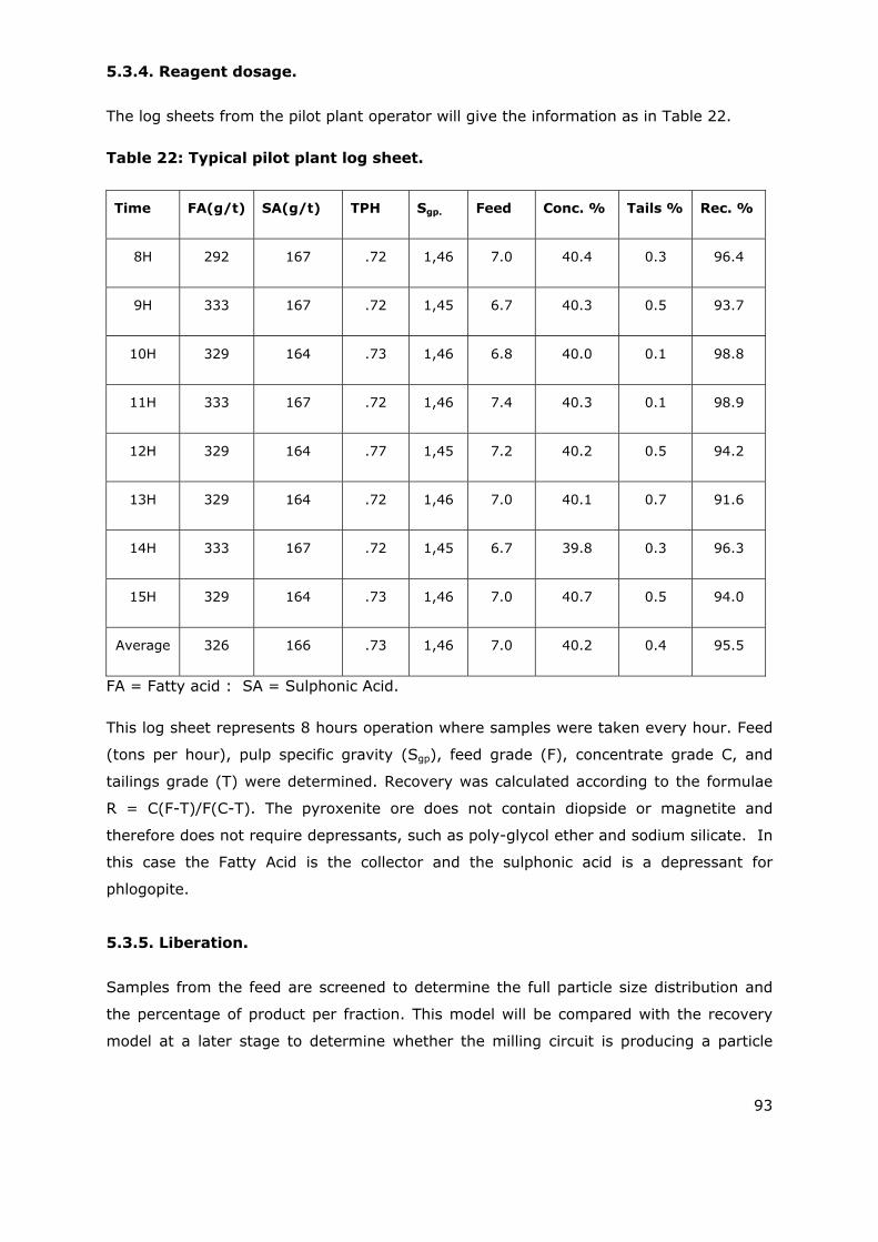
93
5.3.4. Reagent dosage.
The log sheets from the pilot plant operator will give the information as in Table 22.
Table 22: Typical pilot plant log sheet.
Time FA(g/t) SA(g/t) TPH Sgp. Feed Conc. % Tails % Rec. %
8H 292 167 .72 1,46 7.0 40.4 0.3 96.4
9H 333 167 .72 1,45 6.7 40.3 0.5 93.7
10H 329 164 .73 1,46 6.8 40.0 0.1 98.8
11H 333 167 .72 1,46 7.4 40.3 0.1 98.9
12H 329 164 .77 1,45 7.2 40.2 0.5 94.2
13H 329 164 .72 1,46 7.0 40.1 0.7 91.6
14H 333 167 .72 1,45 6.7 39.8 0.3 96.3
15H 329 164 .73 1,46 7.0 40.7 0.5 94.0
Average 326 166 .73 1,46 7.0 40.2 0.4 95.5
FA = Fatty acid : SA = Sulphonic Acid.
This log sheet represents 8 hours operation where samples were taken every hour. Feed
(tons per hour), pulp specific gravity (Sgp), feed grade (F), concentrate grade C, and
tailings grade (T) were determined. Recovery was calculated according to the formulae
R = C(F-T)/F(C-T). The pyroxenite ore does not contain diopside or magnetite and
therefore does not require depressants, such as poly-glycol ether and sodium silicate. In
this case the Fatty Acid is the collector and the sulphonic acid is a depressant for
phlogopite.
5.3.5. Liberation.
Samples from the feed are screened to determine the full particle size distribution and
the percentage of product per fraction. This model will be compared with the recovery
model at a later stage to determine whether the milling circuit is producing a particle
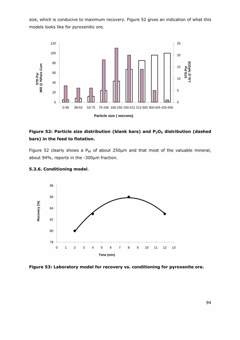
94
size, which is conducive to maximum recovery. Figure 52 gives an indication of what this
models looks like for pyroxenitic ore.
Figure 52: Particle size distribution (blank bars) and P2O5 distribution (dashed
bars) in the feed to flotation.
Figure 52 clearly shows a P80 of about 250µm and that most of the valuable mineral,
about 94%, reports in the -300µm fraction.
5.3.6. Conditioning model.
Figure 53: Laboratory model for recovery vs. conditioning for pyroxenite ore.
0
5
10
15
20
25
0
20
40
60
80
100
120
0-38 38-53 53-75 75-106 106-150 150-212 212-300 300-425 425-500
ST
D.P
yr.L
ib.@
%P
2O
5
ST
D P
yr.M
ill @
%P
ass
Cu
m
Particle size ( microns)
78
80
82
84
86
88
0 1 2 3 4 5 6 7 8 9 10 11 12 13
Rec
ove
ry (
%)
Time (min)
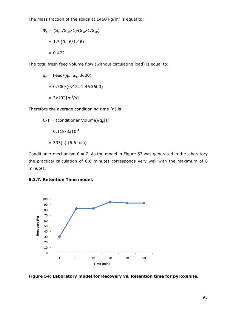
95
The mass fraction of the solids at 1460 kg/m3 is equal to:
Φs = (Sgm/Sgm-1) (Sgp-1/Sgp)
= 1.5 (0.46/1.46)
= 0.472
The total fresh feed volume flow (without circulating load) is equal to;
qp = Feed/(φs Sgp 3600)
= 0.700/(0.472 1.46 3600)
= 3x10⁻⁴[m3/s]
Therefore the average conditioning time (η) is:
C0T = (conditioner Volume)/qp[s]
= 0.118/3x10-4
= 393[s] (6.6 min)
Conditioner mechanism θ = 7. As the model in Figure 53 was generated in the laboratory
the practical calculation of 6.6 minutes corresponds very well with the maximum of 8
minutes.
5.3.7. Retention Time model.
Figure 54: Laboratory model for Recovery vs. Retention time for pyroxenite.
0
10
20
30
40
50
60
70
80
90
100
1 6 12 20 30 50
Rec
ove
ry (
%)
Time (min)

96
Retention time is calculated in the cells where the initial recovery takes place, that is the
roughers and scavengers plus circulating load equal to 30% fresh feed:
τ = (Rougher & Scavenger volume)/qp
= (5 0.085)/(3x10-4 1.3)
= 1089[s] (18.1min)
It is sometimes necessary to make an estimation of the circulating load by consulting the
pump system curves and that must be included in the feed. Again in this case the
practical calculated value corresponded very well with the laboratory results of 20
minutes.
5.3.8. Volumetric Capacity.
The volumetric capacity is defined as:
VC = (Cleaner & Recleaner volume)/(Rougher & Scavenger volume)
= 3 (0.085)/[5 (0.085)]
= 0.6
This value needs to be verified by mass balance calculations. Simple generic models
based on one of the kinetic models produce acceptable results.
5.3.9. Froth Depth.
Figure 55 shows the laboratory results for a pyroxenite mineral and gangue. An
interesting discovery was the behaviour of magnesium and potassium with the two
inflection points at 5% and 10% cell depth. The pilot plant trials showed that the
roughers were running at 10% cell depth and the cleaners were running at 5% cell
depth. This is contradictory to the classical froth depth model and it stresses the point to
analyse for mineral, gangue and secondary gangue. The behaviour of the magnesium
and potassium could not be explained at the time of the experiment. The value of this
discovery was that the contradiction to the classical model could be explained.
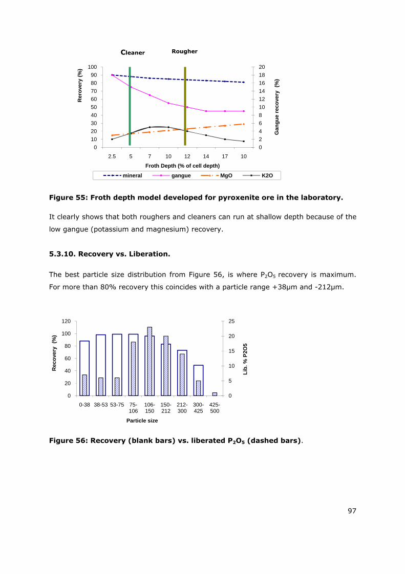
97
Figure 55: Froth depth model developed for pyroxenite ore in the laboratory.
It clearly shows that both roughers and cleaners can run at shallow depth because of the
low gangue (potassium and magnesium) recovery.
5.3.10. Recovery vs. Liberation.
The best particle size distribution from Figure 56, is where P2O5 recovery is maximum.
For more than 80% recovery this coincides with a particle range +38µm and -212µm.
Figure 56: Recovery (blank bars) vs. liberated P2O5 (dashed bars).
0
2
4
6
8
10
12
14
16
18
20
0
10
20
30
40
50
60
70
80
90
100
2.5 5 7 10 12 14 17 10
Gan
gu
e re
cove
ry
(%)
Rer
ove
ry (
%)
Froth Depth (% of cell depth)
mineral gangue MgO K2O
0
5
10
15
20
25
0
20
40
60
80
100
120
0-38 38-53 53-75 75-106
106-150
150-212
212-300
300-425
425-500
Lib
. % P
2O5
Rec
ove
ry
(%)
Particle size
Cleaner Rougher
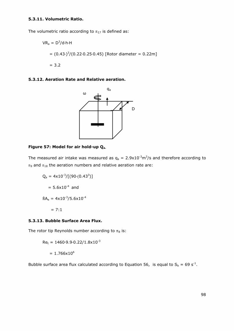
98
5.3.11. Volumetric Ratio.
The volumetric ratio according to 17 is defined as:
VRa = D3/d h H
= (0.43 )3/(0.22 0.25 0.45) [Rotor diameter = 0.22m]
= 3.2
5.3.12. Aeration Rate and Relative aeration.
Figure 57: Model for air hold-up Qa.
The measured air intake was measured as qa = 2.9x10⁻³m3/s and therefore according to
9 and 18 the aeration numbers and relative aeration rate are:
Qa = 4x10⁻³/[(90 0.433)]
= 5.6x10⁻⁴ and
ŘAe = 4x10⁻³/5.6x10-4
= 7:1
5.3.13. Bubble Surface Area Flux. The rotor tip Reynolds number according to 8 is:
Ret = 1460 9.9 0.22/1.8x10-3
= 1.766x10⁶
Bubble surface area flux calculated according to Equation 56, is equal to Sb = 69 s-1.
ω
D
qa
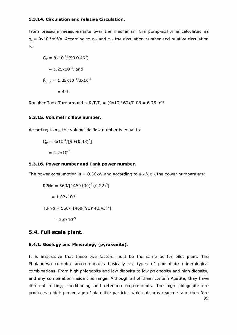
99
5.3.14. Circulation and relative Circulation.
From pressure measurements over the mechanism the pump-ability is calculated as
qc = 9x10⁻³m-3/s. According to 10 and 19 the circulation number and relative circulation
is:
Qc = 9x10⁻³/(90 0.433)
= 1.25x10⁻³, and
Řcirc. = 1.25x10⁻³/3x10-4
= 4:1
Rougher Tank Turn Around is RoTaTu = (9x10⁻³ 60)/0.08 = 6.75 m-1.
5.3.15. Volumetric flow number.
According to 11 the volumetric flow number is equal to:
Qp = 3x10⁻⁴/[90 (0.43)3]
= 4.2x10⁻⁵
5.3.16. Power number and Tank power number. The power consumption is = 0.56kW and according to 15 & 16 the power numbers are:
ŔPNo = 560/[1460 (90)3 (0.22)5]
= 1.02x10⁻³
TaPNo = 560/[1460 (90)3 (0.43)5]
= 3.6x10⁻⁵
5.4. Full scale plant.
5.4.1. Geology and Mineralogy (pyroxenite).
It is imperative that these two factors must be the same as for pilot plant. The
Phalaborwa complex accommodates basically six types of phosphate mineralogical
combinations. From high phlogopite and low diopsite to low phlohopite and high diopsite,
and any combination inside this range. Although all of them contain Apatite, they have
different milling, conditioning and retention requirements. The high phlogopite ore
produces a high percentage of plate like particles which absorbs reagents and therefore
100
require longer conditioning time than the average range. Appendix 6 shows a range of
minerals from the same open pit and the different reagent suites required for each.
5.4.2. Milling and Liberation.
Figure 58: Mineral distribution per fraction.
Figure 58 clearly shows a much higher percentage in the -38 micron fraction and in the
+212µm fraction (Solid bar). About 36% of the P2O5 reports in the low recovery range.
The trend line shows a P80 of about 370µm (Shaded bar).
5.4.3. Chemistry.
Table 23: The chemistry in the main plant.
Reagent Dosage (g/ton)
Fatty Acid 400
Sulphonic Acid 160
The dosage quantity differs from the suite in Table 23 (Pilot plant) The main reason
might be the difference in liberation and interlocked minerals. The depressant seems to
be in the right range but the collector differs more than 25%. This is excessive and
costly.
0
2
4
6
8
10
12
14
16
0
20
40
60
80
100
120
20 38 53 75 106 150 212 300 425
P2O
5 D
istr
ibu
tio
n (
%)
Cu
m p
ass
(%)
Pafrticle size (microns)
101
5.4.4. Operational Conditions.
The section consists of:
2 banks of 8 x roughers + 8 x scavengers of 8.5m3 each.
4 x cleaners + 3 x Recleaners of 4.5m3 each.
The feed is 300 tons per hour per bank at 1350kg/m3 pulp density.
Table 24: Operating parameters for full scale plant.
Parameters Value Dimension
Feed rate per bank 300 Ton.h-1
Aeration rate on roughers 0.04 m3.s-1
Pulp density 1300 kg.m-3
Pulp viscosity 1.7x10⁻³ kg.m-1.s-1
Mineral specific gravity 3 -
Conditioner volume 21 m3
5.4.5. Flow diagram.
The flow diagram is the same as for the pilot plant (Figure 51) except that the cleaners
and recleaners are not the same size machines as the roughers and scavengers.
5.4.6. Conditioning.
The volume flow for the conditioning phase is:
qp = 300/(0.35 1.3 3600)
= 0.18m3/s
Conditioning time:
CoT = 21/0.18
= 116 s (1.9 min)
The conditioner mechanism θ = 3.5/min.
102
5.4.7. Retention time. Volume flow for retention time with 70% circulating load is:
qp = 300 1.7/(0.35 1.3 3600)
= 0.3114(m3/s)
τ = 16 8.5/0.3114
= 436 s (7.2 min)
The volume flow of the circulating load in a full scale plant is too large to measure with
standard containers because of handling problems In this case the use of pump system
curves are the only option though very affective.
5.4.8. Volumetric Capacity.
VC = 7 4.5/16 8.5
= 0.23
5.4.9. Volumetric Ratio.
After inspection it was found that a 144# short rotor was installed which resulted in the
following dimensional set-up:
D = 2.9 m
H = 1.3 m
h = 0.38 m
d = 0.67 m
b = 0.46 m
In the Wemco design the rotor/ draft tube/stand pipe combination represents about 15%
of the total cell volume and therefore one has to consider the effect on diameter and
active volume. The formulae for the volumetric ratio for the Wemco, is reduced to:
VRa = (0.85 2.9)3/(0.67 0.38 1.3)
= 45
103
5.4.10. Rotor tip Reynolds number (Agitation).
From actual measurements the ω = 23.5 r/s (220rpm) and with: vt = 7.9 m/s: p =
1300kg.m3: p = 1.7 x 10⁻³ kg/ms: Rotor diameter = 0.67m then:
Ret = 1350 7.9 0.67/1.7x10-3
= 4.05x10⁶
5.4.11. Volumetric Capacity.
VC = 7 4.5/16 8.5
= 0.23
5.4.12. Aeration number.
The measured aeration rate qa = 0.04m3/s.
Qa = 0.04/[23.5x(2.9 0.85)3]
= 1.14x10⁻⁴
5.4.13. Bubble surface area flux.
From the previous paragraphs the following from Equation 56, the bubble surface area
flux is equal to Sb = 34 s-1.
5.4.14. Circulation number.
According to the Wemco catalogue the circulation is about qc = 0.539 m3/s with clean
water and at Sgp = 1.3 the circulation becomes qc = 0.414 m3/s.
Therefore the circulation number Qc = 0.414/[23 (2.9 0.85)3]
= 1.17x10⁻³
Tank turnaround TaTu = 0.414 60/8.5 = 2.9 min-1.
5.4.15. Volumetric flow.
Qp = 0.3114/23 2.9 0.85)3
= 9x10⁻⁴
104
5.4.16. Power number.
Based on rotor diameter ŔPNo = 28.5x10³/[1300 (23)3 (0.67)5]
= 13.3x10⁻³
Based on cell diameter TaPNo. = 28.5x10³/[1300 (23)3 (2.9 0.85)5]
=1.2x10⁻⁵
5.5. Schedule of dimensionless numbers.
The schedule in Table 25 has been populated with the numerical information calculated
in the preceding paragraphs. The mineralogy and reagent suite is not shown as it is
assumed that these parameters are unchanged. Although the conditioning, retention and
froth depth information has also been developed as dimensionless numbers it is shown
here as dimensional information as it is just practical to display it in the same manner as
the standard production information.
It is obvious from Table 25 that there is very little similarity in almost every metallurgical
and hydrodynamic parameter. This is also summarised by the difference in kinetic
constant. The fact that the power number based on rotor diameter complies, the same
number based on tank diameter demonstrates that the energy requirement is not met.
This set-up performed at a 68% recovery level producing 1850 tons of concentrate per
day at a 7% P2O5 head grade.
5.6. Modified E-Bank.
The flotation banks at Foskor mine are divided into different alphabetical sections which
represented the different minerals as indicated in the mineral spec sheets 1 to 3 in
Appendix 5. The reason is that the different ores have different magnesium and
potassium contents and certain fertilizer processes cannot cope with high magnesium.
E bank processes pyroxenite which has a relatively simple mineralogy and reagent suite.
The full scale comparison under paragraph 5.5 represents the original E-bank
performance which were Wemco 120# with modified 144 rotors. Table 25 shows the
schedule of dimensionless numbers for this condition.
As this bank was at the end of its maintenance life it was decided to replace the old cells
with 21m3 smart cells and to increase cleaner and recleaner capacity. To improve
aeration, bubble surface flux, conditioning time, retention time and grind it was decided
to reduce throughput from 275tph to 240tph and increased RPM from 190 to 200RPM.
Table 26 shows the improvements in operating and dimensionless parameters and Figure
57 and 58 indicate the improvement in performance. Pyroxenite ore contains diopside
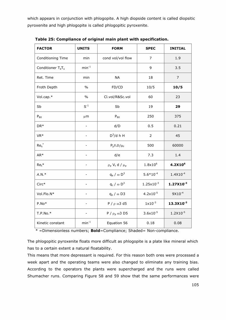
105
which appears in conjunction with phlogopite. A high diopside content is called diopsitic
pyroxenite and high phlogopite is called phlogopitic pyroxenite.
Table 25: Compliance of original main plant with specification.
FACTOR UNITS FORM SPEC INITIAL
Conditioning Time min cond vol/vol flow 7 1.9
Conditioner TaTu min-1 9 3.5
Ret. Time min NA 18 7
Froth Depth % FD/CD 10/5 10/5
Vol.cap.* % Cl.vol/R&Sc.vol 60 23
Sb S-1 Sb 19 29
P80 m P80 250 375
DR* - d/D 0.5 0.21
VR* - D3/d h H 2 45
Res* - ΡpVsD/µp 500 60000
AR* - d/e 7.3 1.4
Ret* - p Vt d / p 1.8x10⁶ 4.2X10⁶
A.N.* - qa / D3 5.6*10-4 1.4X10⁻⁴
Circ* - qc / D3 1.25x10⁻³ 1.27X10⁻³
Vol.Flo.N* - qp / D3 4.2x10⁻⁵ 9X10⁻⁴
P.No* - P / 3 d5 1x10⁻³ 13.3X10⁻³
T.P.No.* - P / p 3 D5 3.6x10⁻⁵ 1.2X10⁻⁵
Kinetic constant min-1 Equation 56 0.18 0.08
* =Dimensionless numbers; Bold=Compliance; Shaded= Non-compliance.
The phlogopitic pyroxenite floats more difficult as phlogopite is a plate like mineral which
has to a certain extent a natural floatability.
This means that more depressant is required. For this reason both ores were processed a
week apart and the operating teams were also changed to eliminate any training bias.
According to the operators the plants were supercharged and the runs were called
Shumacher runs. Comparing Figure 58 and 59 show that the same performances were
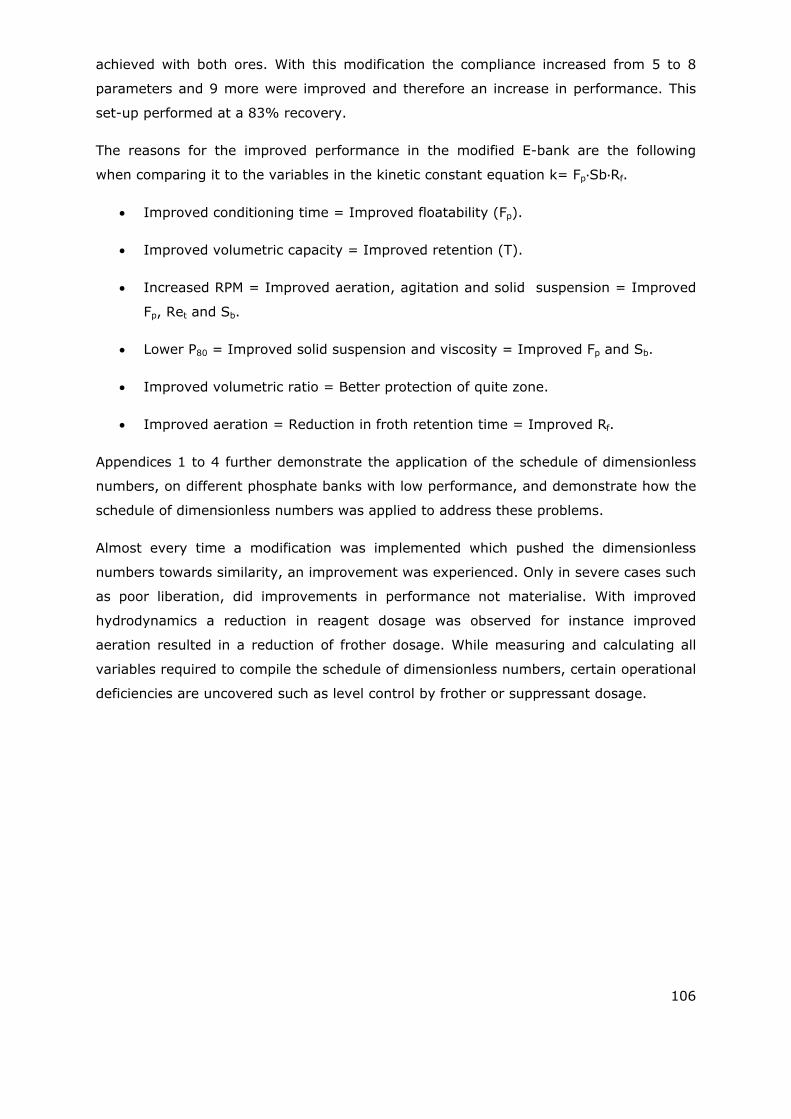
106
achieved with both ores. With this modification the compliance increased from 5 to 8
parameters and 9 more were improved and therefore an increase in performance. This
set-up performed at a 83% recovery.
The reasons for the improved performance in the modified E-bank are the following
when comparing it to the variables in the kinetic constant equation k= Fp Sb Rf.
Improved conditioning time = Improved floatability (Fp).
Improved volumetric capacity = Improved retention (T).
Increased RPM = Improved aeration, agitation and solid suspension = Improved
Fp, Ret and Sb.
Lower P80 = Improved solid suspension and viscosity = Improved Fp and Sb.
Improved volumetric ratio = Better protection of quite zone.
Improved aeration = Reduction in froth retention time = Improved Rf.
Appendices 1 to 4 further demonstrate the application of the schedule of dimensionless
numbers, on different phosphate banks with low performance, and demonstrate how the
schedule of dimensionless numbers was applied to address these problems.
Almost every time a modification was implemented which pushed the dimensionless
numbers towards similarity, an improvement was experienced. Only in severe cases such
as poor liberation, did improvements in performance not materialise. With improved
hydrodynamics a reduction in reagent dosage was observed for instance improved
aeration resulted in a reduction of frother dosage. While measuring and calculating all
variables required to compile the schedule of dimensionless numbers, certain operational
deficiencies are uncovered such as level control by frother or suppressant dosage.
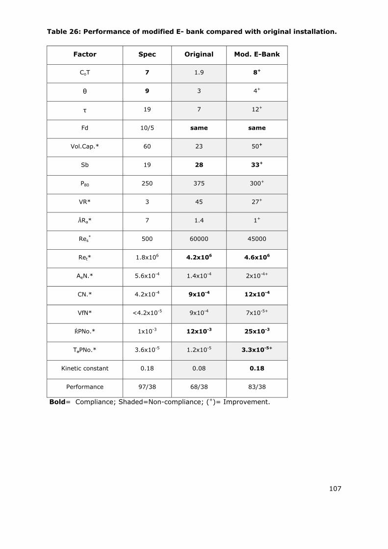
107
Table 26: Performance of modified E- bank compared with original installation.
Factor Spec Original Mod. E-Bank
CoT 7 1.9 8+
θ 9 3 4+
τ 19 7 12+
Fd 10/5 same same
Vol.Cap.* 60 23 50+
Sb 19 28 33+
P80 250 375 300+
VR* 3 45 27+
ÅRa* 7 1.4 1+
Res* 500 60000 45000
Ret* 1.8x106 4.2x10⁶ 4.6x10⁶
AeN.* 5.6x10⁻⁴ 1.4x10⁻⁴ 2x10⁻⁴+
CN.* 4.2x10⁻⁴ 9x10⁻⁴ 12x10-4
VfN* <4.2x10⁻⁵ 9x10⁻⁴ 7x10⁻⁵+
ŔPNo.* 1x10⁻³ 12x10-3 25x10-3
TaPNo.* 3.6x10⁻⁵ 1.2x10⁻⁵ 3.3x10⁻⁵+
Kinetic constant 0.18 0.08 0.18
Performance 97/38 68/38 83/38
Bold= Compliance; Shaded=Non-compliance; (+)= Improvement.
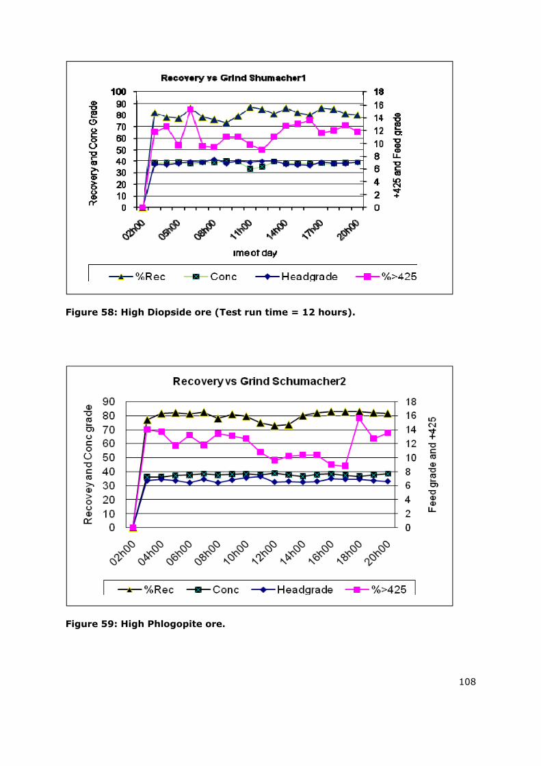
108
Figure 58: High Diopside ore (Test run time = 12 hours).
Figure 59: High Phlogopite ore.

109
CHAPTER 6: APPLICATION OF THE SCHEDULE OF DIMENSIONLESS NUMBERS TO A PLATINUM PLANT.
6.1. The Platinum Industry.
This case study was made difficult by the secrecy between the different South African
platinum producers to protect operational and marketing advantages. Producers are also
reluctant to supply pilot plant information from which to scale-up. Therefore the
specification will be compiled from information gathered in the open literature, from
general flotation requirements and the author’s own experience. The different clients will
also be referred to as Plant 1 and Plant 2. Another difficulty was to obtain an opportunity
to fully apply the schedule of dimensionless to a Platinum plant, therefore this section
will be dedicated to demonstrate how the schedule of dimensionless numbers was
applied to identify deficiencies in these plants.
6.2. Geology.
The Bushveld complex is a massive layered intrusion approximately 2 billion years old,
and is about 350 kilometres in diameter. It intruded through older sedimentary rocks,
some of which contain fossils of the earliest life form. The area of interest for PGM
mineral is a cyclic zone where the rocks are conspicuously layered in a repetitive fashion
referred to as ‘cyclic units’. The base of a cyclic unit is composed of generally dark
coloured minerals, usually pyroxene, olivine or chromite. The layers above these layers
often contain a mixture of these dark minerals with varying proportions of plagioclase
feldspar. These multi-minerallic rocks consist of norite, gabbro, and troctolite.
6.3. Mineralogy.
Two basic mineralogy’s namely Merensky and UG2 are presented in the following
paragraphs.
6.3.1. Merensky.
Table 27: Approximate Merensky mineralogy.
Mineral Pyroxenite Plagioclase Clino Pyr Biotite Talc Others
% 70 20 4 2 small small
110
The Merensky reef is situated in the basalt part of the particular cyclic unit and the
approximate composition is summarised in Table 27. The PGM average composition of
the Merensky minerals, as indicated in Table 28, is 6-9 gm/t.
Table 28: General PGM composition for Merensky.
Mineral Sperrylite Moncheite Cooperite Kotulskite Braggite Pt-Fe Other
% 50 13 10 8 7 6 6
6.3.2. UG2 reef.
The UG2 is the second chromite layer and the approximate composition is outlined in
Table 29.
Table 29: Approximate UG2 mineralogy.
Mineral Chromite Orthopyroxene Plagioclase Magnetite Sulphides
% 75 15 10 small small
The PGM average of the composition as indicated in Table 30 is 4-6 g/t
Table 30: PGM composition for UG2.
Mineral Cooprite Laurite Braggite Sperrylite Pt-Fe
% NKN NKN NKN NKN NKN
NKN = Not Known
6.4. Flotation chemistry.
The reagent suite for the flotation of minerals from the Merensky and UG2 reefs is
summarised in Table 31.
Table 31: Reagent suite for Merensky and UG2 (g/t).
Reef SIBX FROTH PROM ACT DEPR
Merensky 30 30 70 - 70
UG2 35 100 - - 25
111
6.5. Operational Considerations.
The presence of talc in Merensky minerals requires special depressants and grinding
control as talk mills fine easily and therefore has a natural floatability. The depressant in
this case is normally a 10% starch solution. Chromite on the other hand will mill with
more difficulty and having a high density will require special pumping and solid
suspension requirements.
6.5.1. Conditioning.
An unconventional approach found in the platinum industry is that conditioning is
replaced by stepwise dosage. This is the only industry where intimate mixing of the
solids and reagents are not required as the tank turn around (Circulation) of flotation
machines are far to low for this purpose. This approach also unnecessarily consumes
precious retention time. About 20 minutes conditioning time is required for
nickel/copper/pgm combinations and there is no reason why this won’t work for
Merensky and UG2. Minerals.
6.5.2. Retention.
General requirements for retention times are summarised in Table 32.
Table 32: Retention times for Merensky and UG2 (min).
Cycle Primary
Rougher
Primary
Cleaner
Primary
Re-cleaner
Secondary
Rougher
Secondary
Cleaner
Secondary
Re-cleaner
Time (min) 30 60 60 30 60 60
This seems to correspond well with other plants with the same mass balance
requirements.
6.5.3. Flow Diagrams.
The general flow diagram in the Platinum industry is one of grind/float/grind/float. The
primary concentrates from the first rougher, cleaner and recleaner are normally final
concentrates, and cleaners and recleaners are scavenging on themselves.
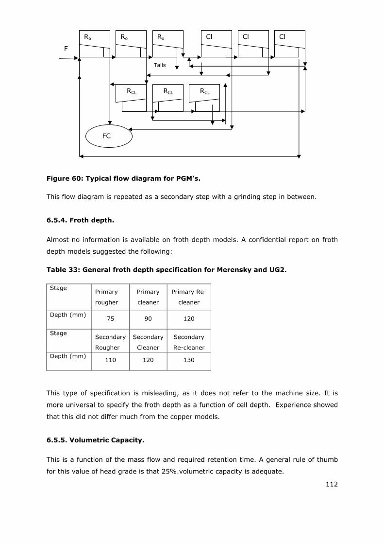
112
Figure 60: Typical flow diagram for PGM’s.
This flow diagram is repeated as a secondary step with a grinding step in between.
6.5.4. Froth depth.
Almost no information is available on froth depth models. A confidential report on froth
depth models suggested the following:
Table 33: General froth depth specification for Merensky and UG2.
Stage Primary
rougher
Primary
cleaner
Primary Re-
cleaner
Depth (mm) 75 90 120
Stage Secondary
Rougher
Secondary
Cleaner
Secondary
Re-cleaner Depth (mm)
110 120 130
This type of specification is misleading, as it does not refer to the machine size. It is
more universal to specify the froth depth as a function of cell depth. Experience showed
that this did not differ much from the copper models.
6.5.5. Volumetric Capacity.
This is a function of the mass flow and required retention time. A general rule of thumb
for this value of head grade is that 25%.volumetric capacity is adequate.
FC
Ro Ro Ro Cl Cl Cl
RCL RCL RCL
F
Tails
113
6.5.6. Volumetric ratio, Superficial and Rotor Reynolds number.
The general scale-up specification applies. The dimensionless number for this ratio is
4 < VRa < 16, Res < 15x103 and 4x10⁶ < Ret > 7x10⁶.
6.5.7. Circulation.
The circulation capability of the machine depends on the sinking velocity of the top 5%
of particle size. This can be specified as:
Table 34: Tank turn around.
6.5.8. Aeration and Bubble surface area flux and Power numbers.
The aeration and bubble surface area flux requirements are as indicated in Table 35.
Table 35: Aeration and bubble surface flux for Merensky and UG2.
6.6. Schedule of dimensionless numbers.
The analysis shows that very little similarity was maintained during the design stage.
The deficiencies could be summarised as follows:
Some uncertainty exists, regarding exact reagent suite, as these companies are
very sensitive in divulging this type of information. For some of them this
information is highly secret.
No liberation model, froth depth model and recovery vs. particle size model
conditioning time and retention time models existed in some cases. The
specification for comparison was decided upon after deliberation with research
personnel and normally resulted in a combination of the laboratory and pilot plant
information produced in the Foskor plant for a very low head grade copper
Circulation Tank Turn-around
4.3x10⁻⁴ 3 – 4
Aeration Number
(AeN)
Bubble surface area
flux (Sb) Tank power number
4.1x10⁻⁴ 90 s-1 4.2x10⁻⁵
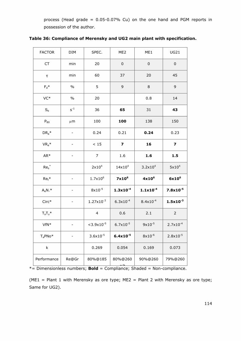
114
process (Head grade = 0.05-0.07% Cu) on the one hand and PGM reports in
possession of the author.
Table 36: Compliance of Merensky and UG2 main plant with specification.
FACTOR DIM SPEC. ME2 ME1 UG21
CT min 20 0 0 0
τ min 60 37 20 45
Fd* % 5 9 8 9
VC* % 20 0.8 14
Sb s-1 36 65 31 43
P80 m 100 100 138 150
DRa* - 0.24 0.21 0.24 0.23
VRa* - < 15 7 16 7
AR* - 7 1.6 1.6 1.5
Res* 2x104 14x104 3.2x10⁴ 5x10⁴
Ret* - 1.7x10⁶ 7x10⁶ 4x10⁶ 6x10⁶
AeN.* - 8x10⁻⁵ 1.3x10⁻⁴ 1.1x10⁻⁴ 7.8x10⁻⁵
Circ* - 1.27x10⁻³ 6.3x10⁻⁴ 8.4x10⁻⁴ 1.5x10⁻³
TaTu* 4 0.6 2.1 2
VfN* - <3.9x10⁻⁵ 6.7x10⁻⁵ 9x10⁻⁵ 2.7x10⁻⁴
TaPNo* - 3.6x10⁻⁵ 6.4x10⁻⁵ 8x10⁻⁶ 2.8x10⁻⁵
k 0.269 0.054 0.169 0.073
Performance Re@Gr 80%@185 80%@260
g/t
90%@260 79%@260
*= Dimensionless numbers; Bold = Compliance; Shaded = Non-compliance.
(ME1 = Plant 1 with Merensky as ore type; ME2 = Plant 2 with Merensky as ore type;
Same for UG2).
115
Too high superficial Reynolds number. The superficial Reynolds number is a tool
to decide on the number of parallel lines. It is possible to design plants with less
units in series with the new tank cells as these cells are no longer open channels
and short circuiting are limited in these designs. More parallel banks will reduce
the superficial velocity and the superficial Reynolds numbers and force it towards
similarity.
Too low aeration and bubble surface flux. The supply are normally external
aeration and the aeration number is below the numerical value for similarity.
Bubble surface area flux is between 40-60 s-1 and this is also below the process
specification.
Too low circulation. This can lead to the settlement of solid particles.
Too high volumetric flow. This represents a dimensionless retention time and is
supported by the actual retention time which is below specification. This is
evident in plants where production is increased to increase output. This normally
happens when the product prise is high.
116
CHAPTER 7: CALE-UP METHODOLOGY.
7.1. New scale-up algorithm.
7.1.1. Assumptions.
Before running the algorithm the following information must be known:
Conditioning and retention times
Required particle size distribution
Type of design: High or low aspect ratio
7.1.2. Algorithm.
See detail algorithm in Appendix 8.
7.2. Discussion of new algorithm.
7.2.1. The calculations in step 1 to 3 follows from the standard plant calculations in §3.10.
7.2.2. In step 4 the rotor RPM is calculated by applying the adjusted transformation
number generated in Equation 36 namely FrRGA = idem.
7.2.3. In step 5 the power requirement is based on the Tank power number and the
rotor power number is adjusted with the ratios of rotor heights for comparison
with the pilot plant. The reason for the adjustment with the ratio of rotor heights
is because the full scale rotor is viewed as a multi-stage version of the pilot plant
rotor. If the full scale rotor was simply an adjustment of diameter then the affinity
laws would have applied
7.2.4. In step 6 the circulation is again based on tank diameter and adjustment with the
ratio of rotor heights for the same reason as in §7.2.3.
7.2.5. Step 7 represents the calculation of the agitation level based on rotor tip Reynolds
number. To compare with pilot plant agitation the Reynolds number is adjusted
with the ratio of relative particle size according to Mavros (1992).
117
7.2.6. Step 8 the dimensionless numbers are compared in the schedule format.
7.2.7. Finally the kinetic constant and its parameters are calculated according to
Equations (46) to (62). The reasoning is that with retention time and kinetic
constant = idem than the recovery should be the same
7.3. Application of the new algorithm to a standard industrial design.
7.3.1. Table 37 shows the related dimensionless numbers that must also be kept
constant. The froth depth number FD/H = idem is required to ensure the same
concentrate grade. In this case the as there are no conditioning in this plant the
dimensionless conditioning parameters ωθ = idem and ωη = idem were both set
equal to 1.
Table 37: The following dimensionless numbers are =idem.
Relative
Particle
size
Relative froth depth
Conditioning time
Tank turn around
Froth
retention
time
Superficial
Reynolds
number
P80/D Fd/H ωη ωθ ωξ ρPJpD/μP
7.3.2. Table 38 shows the comparison between a pilot plant used for sulphide and non-
metal floats and a 50 cubic meter cell as these designs are actively in service in
the South African PGM mining industry. This machine has been installed as a
rougher stage on a UG2 plant. With the improvement of rotor diameter from
0.99m to 1.16m and reducing RPM from 14r/s to 12r/s complied with the
transformation requirements and resulted in an improvement of all operating and
dimensionless parameters as well as a 31% improvement in floatability
parameter, a 1.6% improvement in froth recovery and almost 200%
improvement in the kinetic constant and end in an expected improvement of 7%
points in recovery.
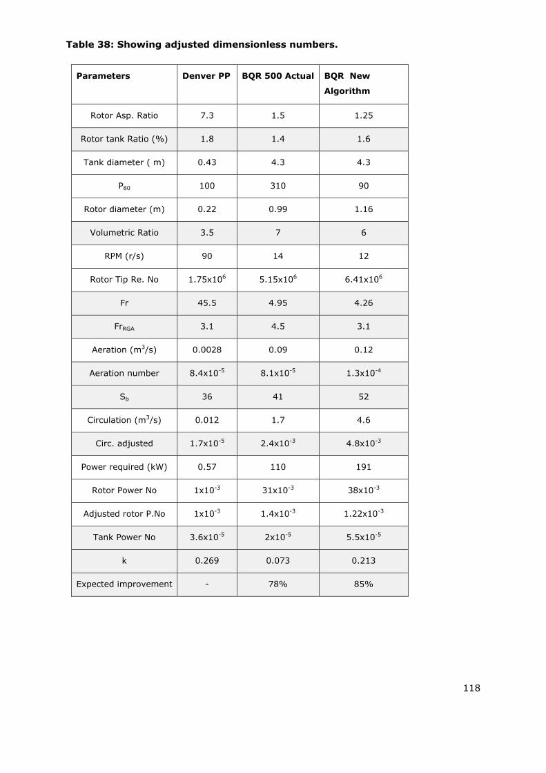
118
Table 38: Showing adjusted dimensionless numbers.
Parameters Denver PP BQR 500 Actual BQR New
Algorithm
Rotor Asp. Ratio 7.3 1.5 1.25
Rotor tank Ratio (%) 1.8 1.4 1.6
Tank diameter ( m) 0.43 4.3 4.3
P80 100 310 90
Rotor diameter (m) 0.22 0.99 1.16
Volumetric Ratio 3.5 7 6
RPM (r/s) 90 14 12
Rotor Tip Re. No 1.75x10⁶ 5.15x10⁶ 6.41x10⁶
Fr 45.5 4.95 4.26
FrRGA 3.1 4.5 3.1
Aeration (m3/s) 0.0028 0.09 0.12
Aeration number 8.4x10⁻⁵ 8.1x10⁻⁵ 1.3x10⁻⁴
Sb 36 41 52
Circulation (m3/s) 0.012 1.7 4.6
Circ. adjusted 1.7x10⁻⁵ 2.4x10⁻³ 4.8x10⁻³
Power required (kW) 0.57 110 191
Rotor Power No 1x10⁻³ 31x10-3 38x10-3
Adjusted rotor P.No 1x10⁻³ 1.4x10⁻³ 1.22x10⁻³
Tank Power No 3.6x10⁻⁵ 2x10⁻⁵ 5.5x10⁻⁵
k 0.269 0.073 0.213
Expected improvement - 78% 85%
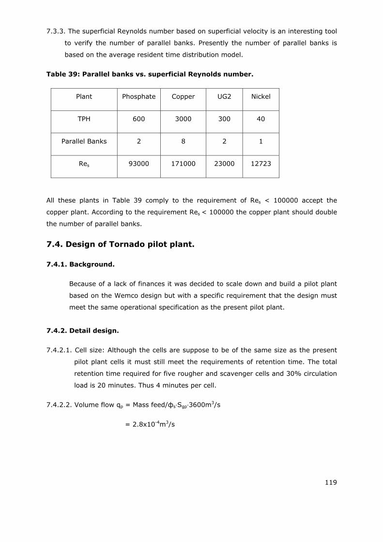
119
7.3.3. The superficial Reynolds number based on superficial velocity is an interesting tool
to verify the number of parallel banks. Presently the number of parallel banks is
based on the average resident time distribution model.
Table 39: Parallel banks vs. superficial Reynolds number.
Plant Phosphate Copper UG2 Nickel
TPH 600 3000 300 40
Parallel Banks 2 8 2 1
Res 93000 171000 23000 12723
All these plants in Table 39 comply to the requirement of Res < 100000 accept the
copper plant. According to the requirement Res < 100000 the copper plant should double
the number of parallel banks.
7.4. Design of Tornado pilot plant.
7.4.1. Background.
Because of a lack of finances it was decided to scale down and build a pilot plant
based on the Wemco design but with a specific requirement that the design must
meet the same operational specification as the present pilot plant.
7.4.2. Detail design.
7.4.2.1. Cell size: Although the cells are suppose to be of the same size as the present
pilot plant cells it must still meet the requirements of retention time. The total
retention time required for five rougher and scavenger cells and 30% circulation
load is 20 minutes. Thus 4 minutes per cell.
7.4.2.2. Volume flow qp = Mass feed/фs Sgp 3600m3/s
= 2.8x10⁻⁴m3/s
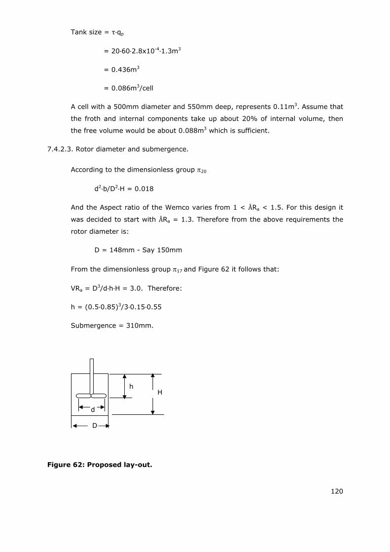
120
Tank size = τ qp
= 20 60 2.8x10⁻⁴ 1.3m3
= 0.436m3
= 0.086m3/cell
A cell with a 500mm diameter and 550mm deep, represents 0.11m3. Assume that
the froth and internal components take up about 20% of internal volume, then
the free volume would be about 0.088m3 which is sufficient.
7.4.2.3. Rotor diameter and submergence.
According to the dimensionless group 20
d2 b/D2 H = 0.018
And the Aspect ratio of the Wemco varies from 1 < ÅRa < 1.5. For this design it
was decided to start with ÅRa = 1.3. Therefore from the above requirements the
rotor diameter is:
D = 148mm - Say 150mm
From the dimensionless group 17 and Figure 62 it follows that:
VRa = D3/d h H = 3.0. Therefore:
h = (0.5 0.85)3/3 0.15 0.55
Submergence = 310mm.
Figure 62: Proposed lay-out.
h H
d
D
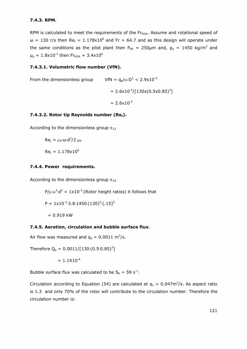
121
7.4.3. RPM.
RPM is calculated to meet the requirements of the FrRGA. Assume and rotational speed of
ω = 130 r/s then Ret = 1.178x10⁶ and Fr = 64.7 and as this design will operate under
the same conditions as the pilot plant then P80 = 250μm and, ρp = 1450 kg/m3 and
μp = 1.8x10⁻³ then FrRGA = 3.4x10⁶
7.4.3.1. Volumetric flow number (VfN).
From the dimensionless group VfN = qp/ D3 < 2.9x10-5
= 2.6x10⁻⁴/[130x(0.5x0.85)3]
= 2.6x10⁻⁵
7.4.3.2. Rotor tip Reynolds number (Ret).
According to the dimensionless group 12
Ret = P ω d2/2 P
Ret = 1.178x10⁶
7.4.4. Power requirements.
According to the dimensionless group 14
P/ 3 d5 = 1x10⁻³ (Rotor height ratios) it follows that
P = 1x10⁻³ 3.8 1450 (130)3 (.15)5
= 0.919 kW
7.4.5. Aeration, circulation and bubble surface flux. Air flow was measured and qa = 0.0011 m3/s.
Therefore Qa = 0.0011/[130 (0.5 0.85)3]
= 1.1X10⁻⁴
Bubble surface flux was calculated to be Sb = 59 s-1.
Circulation according to Equation (54) are calculated at qc = 0.047m3/s. As aspect ratio
is 1.3 and only 70% of the rotor will contribute to the circulation number. Therefore the
circulation number is:
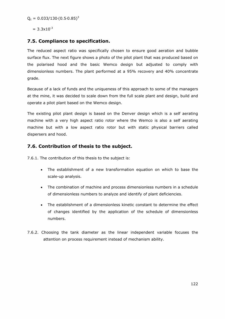
122
Qc = 0.033/130 (0.5 0.85)3
= 3.3x10⁻³
7.5. Compliance to specification.
The reduced aspect ratio was specifically chosen to ensure good aeration and bubble
surface flux. The next figure shows a photo of the pilot plant that was produced based on
the polarised hood and the basic Wemco design but adjusted to comply with
dimensionless numbers. The plant performed at a 95% recovery and 40% concentrate
grade.
Because of a lack of funds and the uniqueness of this approach to some of the managers
at the mine, it was decided to scale down from the full scale plant and design, build and
operate a pilot plant based on the Wemco design.
The existing pilot plant design is based on the Denver design which is a self aerating
machine with a very high aspect ratio rotor where the Wemco is also a self aerating
machine but with a low aspect ratio rotor but with static physical barriers called
dispersers and hood.
7.6. Contribution of thesis to the subject.
7.6.1. The contribution of this thesis to the subject is:
The establishment of a new transformation equation on which to base the
scale-up analysis.
The combination of machine and process dimensionless numbers in a schedule
of dimensionless numbers to analyze and identify of plant deficiencies.
The establishment of a dimensionless kinetic constant to determine the effect
of changes identified by the application of the schedule of dimensionless
numbers.
7.6.2. Choosing the tank diameter as the linear independent variable focuses the
attention on process requirement instead of mechanism ability.
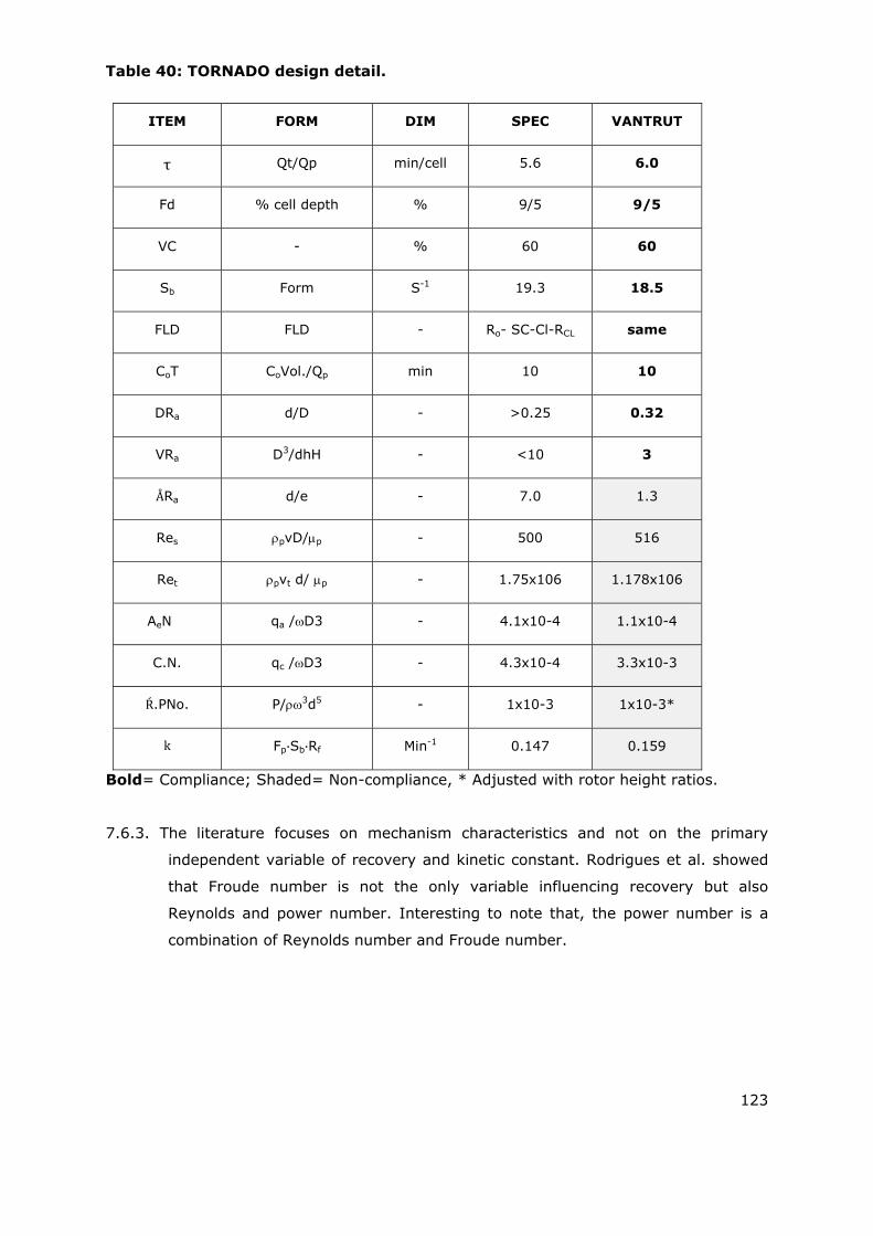
123
Table 40: TORNADO design detail.
ITEM FORM DIM SPEC VANTRUT
τ Qt/Qp min/cell 5.6 6.0
Fd % cell depth % 9/5 9/5
VC - % 60 60
Sb Form S-1 19.3 18.5
FLD FLD - Ro- SC-Cl-RCL same
CoT CoVol./Qp min 10 10
DRa d/D - >0.25 0.32
VRa D3/dhH - <10 3
ÅRa d/e - 7.0 1.3
Res pvD/p - 500 516
Ret pvt d/ p - 1.75x10⁶ 1.178x10⁶
AeN qa /D3 - 4.1x10⁻⁴ 1.1x10⁻⁴
C.N. qc /D3 - 4.3x10⁻⁴ 3.3x10⁻³
Ŕ.PNo. P/3d5 - 1x10⁻³ 1x10⁻³*
k Fp Sb Rf Min-1 0.147 0.159
Bold= Compliance; Shaded= Non-compliance, * Adjusted with rotor height ratios.
7.6.3. The literature focuses on mechanism characteristics and not on the primary
independent variable of recovery and kinetic constant. Rodrigues et al. showed
that Froude number is not the only variable influencing recovery but also
Reynolds and power number. Interesting to note that, the power number is a
combination of Reynolds number and Froude number.
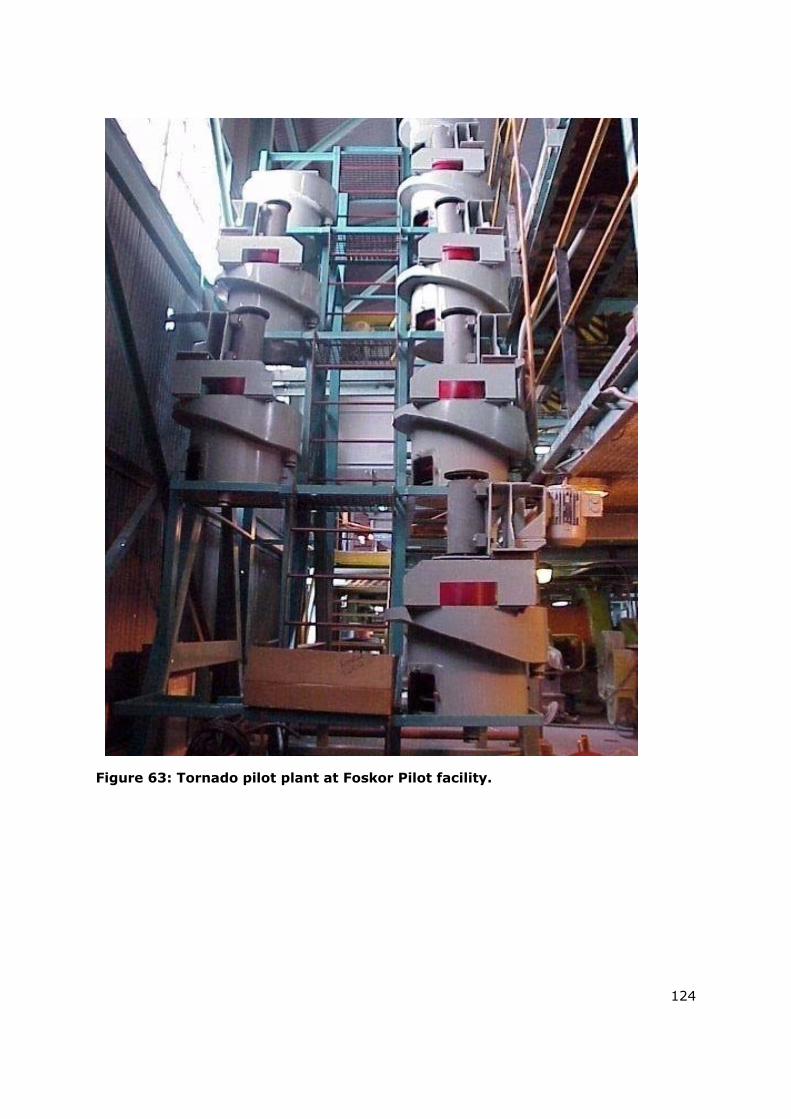
124
Figure 63: Tornado pilot plant at Foskor Pilot facility.
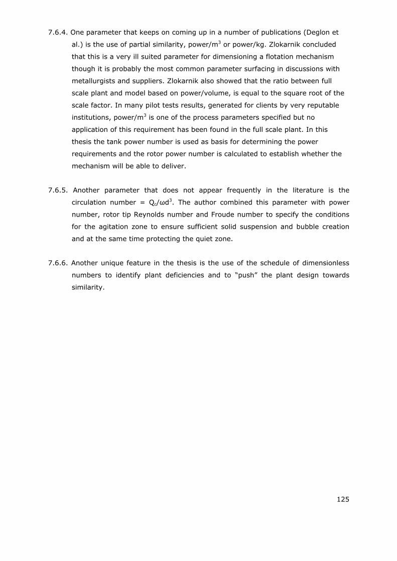
125
7.6.4. One parameter that keeps on coming up in a number of publications (Deglon et
al.) is the use of partial similarity, power/m3 or power/kg. Zlokarnik concluded
that this is a very ill suited parameter for dimensioning a flotation mechanism
though it is probably the most common parameter surfacing in discussions with
metallurgists and suppliers. Zlokarnik also showed that the ratio between full
scale plant and model based on power/volume, is equal to the square root of the
scale factor. In many pilot tests results, generated for clients by very reputable
institutions, power/m3 is one of the process parameters specified but no
application of this requirement has been found in the full scale plant. In this
thesis the tank power number is used as basis for determining the power
requirements and the rotor power number is calculated to establish whether the
mechanism will be able to deliver.
7.6.5. Another parameter that does not appear frequently in the literature is the
circulation number = Qc/ωd3. The author combined this parameter with power
number, rotor tip Reynolds number and Froude number to specify the conditions
for the agitation zone to ensure sufficient solid suspension and bubble creation
and at the same time protecting the quiet zone.
7.6.6. Another unique feature in the thesis is the use of the schedule of dimensionless
numbers to identify plant deficiencies and to “push” the plant design towards
similarity.
126
CHAPTER 8: CONCLUSIONS AND RECOMMENDATION.
8.1. Dimensionless analysis.
This thesis is unique in addressing the transformation number, kinetic constant
and dimensionless schedule at the same time. Comparing the transformation
equation with standard industrial machines clearly showed that that these designs
did not follow the scale-up criteria of Fr = idem. Most of these designs , especially
the Wemco design, followed partial similarity of kW/m3 = idem or
Ret Fr0.5 G0.45 ÅRa-0.2 = idem
The establishing of an equation for the kinetic constant based on dimensionless
numbers resulted in a model built on about 16 variables. The application of this
model to different designs and minerals seems to produce acceptable results.
The validation of floatability parameter and froth recovery factor needs more
attention. In this analysis the author did not try to generate dimensionless
relationships for entrainment and drainage as these are implied in the overall
kinetic constant. Entrainment has a detrimental effect on concentrate grade and
in this case the grade is fixed by the froth depth. In this case the approach was
rather to create conditions that are conducive for froth phase protection and fine
particle collision conditions.
8.2. Schedule of Dimensionless numbers.
It has also been found that the schedule of dimensional numbers is a relative
simple method entailing simple measurements, calculations and comparisons. It
does not require complicated measuring equipment or special conditions but
simple production and maintenance tools.
Finally it amounts to a simple comparison between simple ratios which then
creates the opportunity to identify and rectify these deficiencies by entertaining
improvements that will force the plant towards similitude. The deviation from the
basic transformation equation of Fr = idem might have something to do with
economics of the time though many of these machines were designed and
installed when this relationship was well known.

127
8.3. Main plant performance.
It is true that full scale plants perform much worse than pilot plants to as much
as 30%. These deficiencies are also independent of machine or mineral. The
same deficiencies have been found in copper, phosphate, nickel, platinum and
carbonate plants.
These plants utilised the full range of equipment, with different sizes, self-
aerating or external aerating machines, low and high aspect ratio rotors and high
and low volumetric ratio though the deficiencies are the same.
8.4. Process Characterization.
After discussions with metallurgists and research engineers regarding the scale-
up methodology applied in their full scale designs, it percolated that they put a lot
of effort in characterising the process by compiling mineralogical, metallurgical
and chemical specifications and then turn it over to the suppliers of equipment to
supply the appropriate equipment based on a single characteristic such as power/
cubic metre. No where did the author find any hydrodynamic characteristics as
part of the specification. The reason is that these metallurgists work in isolation
with hardly any assistance from engineers. When one enquires about the
hydrodynamic characteristics of these machines the author discovered that it
exists only partially. The basis for selecting a specific machine is most of the time
based on that which worked somewhere else.
The application of dimensional similitude clearly demonstrated the simplicity of
this methodology. It highlighted almost ten major deficiencies such as aeration
numbers, rotor tip Reynolds number, power number, circulation number etc, in
every plant. At most plants a lot of effort is put into the testing of reagents and
the reason is that it is one of the highest cost items but very little time is spent
on the fundamental issues of flotation such as kinetic activity and what variables
influence its value.
8.5. Process specification.
In certain cases in the industry, processes have been design by “stealing” with
the eyes and ears from other existing plants. Major flotation plants have been
designed and built this way. When requesting process information to determine
whether the plant has been constructed to specification, none was available. This
clearly demonstrated the none-existence of any scale-up technique during the
design of these full scale plants.

128
8.6. Scale-up Techniques.
Most scale-up techniques are proposals but with no prove of analysis, identification
of deficiencies, suggested improvements, prediction of success and
implementation. Most plants were either duplication of existing designs where the
same deficiencies were repeated or some copy of another similar plant.
8.7. CFD results of Wemco machine.
The following has been established in this simulation of the mineral recovery rate
of the WEMCO 120 flotation cell:
The trajectories of the air bubbles are driven by buoyancy once they are out of
the high fluid velocity area. The trajectories of the solid particles are driven by
and follow the continuous liquid phase throughout the flotation cell. The solid
particle sedimentation is as expected concentrated on the bottom and false floors.
An effective procedure has been established to apply field measured data of
recovery rates to the computational domain. This interpolated recovery rate
values have proved effective to evaluate other important flow parameters in
particular the pulp and bubble Reynolds numbers and the bubble-particle collision
frequency. The most important results from the present work are the evidence
that the bubble-particle collision frequency follows the same trend as the
interpolated recovery rate values. Since these values are unrelated, one being
interpolated from measured values and the other derived from theory one may
safely continue to investigate the importance of this parameter. The same applies
to the relevance of the bubble Reynolds number. This parameter has shown that
the slip velocity between bubbles and liquid phase may be more important than
the pulp velocity. This may be justified by the fact that initial bubble-particle
collision can only take place if such a slip velocity exists, a fact inherent to the
theory underlying the expression for the bubble-particle collision frequency.
It has been shown that there exists good agreement between the interpolated
measured recovery rate data and a local recovery rate found by using the bubble-
particle collision frequency. The bubble Reynolds number has also shown to follow
the same trend as the interpolated recovery rate values. It is suggested that
more detailed evaluation of these trends are made correlating the CFD prediction
of bubble-particle collision frequency and bubble Reynolds number to the
interpolated recovery rate data. At this stage the bubble-collision frequency
theory only predicts the probability of initial bubble-particle collisions and does
not provide information on whether the solid particles will remain attached.
129
Global mineral recovery rate from CFD field results. This could be achieved by
developing a method to predict the overall recovery rate potential of the flotation
cell by utilising the data predicted by the CFD simulation. This data should be
interpreted and a method proposed.
130
ABBREVIATIONS.
ACT = Activator.
AP = Apatite.
ÅRa = Rotor aspect ratio.
Ar = Archimedes number.
Conc. = Concentrate.
Circ= Circulation.
CAL = Calcite.
CFD = Computational fluid dynamics.
Cl = Cleaner.
CN = Circulation number.
CUM = Cumulative.
Cu 1-2 = Different copper plants.
DEPR = Depressant.
DIOP = Diopsite.
DIM = Dimension.
DRa = Diameter ratio.
FA = Fatty acid.
FC = Final concentrate.
FLD = Flow diagram.
FOR = Forsterite.
FRT =Dimensionless froth retention time.
FSP = Full scale plant.
FC = Final concentrate grade (%).
131
G = Relative particle size ratio.
Idem = Identical value.
Lib = Liberation.
LIZ = Lizerdite.
MAG = Magnetite.
Mill = Milling (Grinding.)
Ne = Newton number.
PGM 1-2 = Different platinum plants.
PHL = Phlogopite.
PP = Pilot plant.
Pyr = Pyroxenite ore.
PROM = Promoter.
RCL = Recleaner.
REC = Recovery.
ŔPNo.= Rotor power number.
ŔTaVRa = Rotor tank volumetric ratio.
RTD = Residence time distribution.
SA = Sulphonic acid.
Sc = Scavenger.
STD = Standard.
Tails = Tailings.
Tmf = Tails mass flow.
TaPNo= Power number based on tank diameter.
TaSRa = Tank slenderness ratio.
TaTu = Tank-turn-round.
132
TPH = Tons per hour.
VC = Volumetric capacity (%).
VfN = Volumetric flow number.
VRa = Volumetric Ratio.
VC = Volumetric capacity.
VERM = Vermiculite.
133
NOMENCLATURE.
Symbols.
Ac = Cell area (m2).
AeN = Aeration number.
Asi = Stand pipe inlet area (m2).
a-c = Streamline identification in potential flow.
a’-c’ = Streamline identification in potential flow.
B = Reference length in the weir equation (m).
Cd = Drag coefficient.
CoT = Conditioning time (min).
d = Rotor diameter (m).
db = Bubble diameter (m).
dm = Mineral particle diameter (m).
d32 = Sauter diameter (m).
D = Tank diameter (m) (Reference diameter).
Dh = Hydraulic diameter (m).
b = Rotor height (m).
ft = Transformation equations.
f1 –f5 = Functions.
F = Feed rate (Tph).
Fb = Buoyancy force (N).
Fcd = Drag force (N).
Fd = Froth depth (%).
Fg = Gravitational force (N).
134
Fo = Force (N).
Fp = Floatability parameter in kinetic constant.
Fr = Froude number.
FrD = Froude number based on tank diameter D.
Fr* = Froude number combined with Reynolds number.
Fr’ = Special adapted Froude number.
FrRGA = Froude number combined with Reynolds number, relative particle size ratio and
rotor aspect ratio.
g = Gravitational constant (9.81 m/s2).
G = Ratio between relative particle size for full scale plant and pilot plant..
h = Rotor submergence (m).
h* = Distance of stirrer from bottom of tank (m).
H = Tank height (m).
H* = Filling height (m).
Hw = Water height in weir flow equation (m).
i = Constant in froth recovery factor.
j = Drainage constant in froth recovery factor.
Jg = Superficial velocity (cm/s).
Jp = Superficial pulp velocity (m/s).
k = Kinetic constant (min-1).
k’ = Kinetic constant modified with VRa (min-1).
k’’ = Constant in propeller blade equation.
ka = Attachment rate constant.
kd = De-attachment rate constant.
k = Numerical value of kinetic constant.
135
l = Pipe length in pipe flow equation (m).
m = Number of variables in - theorem.
n = Number of fundamental dimensions.
n’ = Constant in circulation equation for the Wemco machine.
n’’ = Number of tanks in series.
Nc = Critical speed for rotating equipment.
Nm = Mineral particle number in collision model.
Na = Air bubble number in collision model.
Ne = Newton number.
P = Power.
P80 = Screen size of which 80% will pass (µm) Q = Volume flow (m3/s).
qa = Aeration rate (m3/s).
qc = Circulation rate (m3/s).
qacv = Air flow in control volume in CFD model. (m3/s).
qp = Pulp volume feed rate (m3/s).
qpcv = Pulp flow rate in control volume in CFD model (m3/s).
qrva = Local relative aeration rate in CFD model.
Q = Volume flow (m3/s).
Qa = Aeration number.
Qc = Circulation number.
Qp = Pulp flow number.
Qrrp = Recovery rate potential function.
Qt = Tank volume (m3).
Q1, Q2-Qm = System variables.
rc = Radius of chanel where flow is equal to vr.
136
ro = Radius of channel (m).
R = Recovery (%)
ŘAe = Relative aeration rate.
RCLC = Recleaner capacity (%).
ŘFd = Relative froth depth.
Řcirc = Relative circulation.
Řps = Relative particle size.
Res = Superficial Reynolds number.
Re = Reynolds number.
Res = Superficial Reynolds number.
Ret = Rotor tip Reynolds number.
Reb = Bubble Reynolds number.
Recv = Reynolds number of local control volume in CFD model.
Rf = Froth recovery factor.
Rh = Rotor height (m).
Rm = Maximum expected recovery (%).
Ro = Rougher.
S = Maximum expected recovery in Klimple model (%).
Sa = Scale factor.
Sb = Bubble surface flux (sec-1).
Sbmax = Maximum bubble surface area flux (sec-1).
Sgs = Specific gravity of solids.
Sgp = Specific gravity of pulp.
Sgcv = Specific gravity of control volume in CFD model.
t = Real time (minutes).
137
T = Tailings.
Te = Temperature (OK).
U = Forward velocity (m/s).
U1 = Inlet velocity (m/s).
U2 = Outlet velocity (m/s).
Uf = Liquid phase velocity (m/s).
Ua = Air phase relative velocity (m/s).
Um = Solid phase relative velocity (m/s).
v = Linear forward velocity (m/s).
va = Average impeller air inlet velocity (m/s).
vacv = Local air speed at control volume (m/s).
vpcv = Local pulp velocity (m/s).
vo = Free stream velocity (m/s).
vp = Average outlet pulp velocity (m/s).
vr = Velocity at distance r (m/s).
vt= Rotor tip velocity (m/s).
vs = Sinking velocity (m/s).
Vcv = Volume of control volume in CFD analysis (m3).
We = Weber number.
x1 – x4 = Unknown exponents in equation for propeller blade.
x’ = Exponent in equation for aeration in Wemco machine.
y1 – y4 = Unknown constants in equation for pipe flow based on Rayleigh’s indicial
method.
y’ = Function of independent variables.
y’’ = Deflection in critical speed for rotary equipment (m)
138
z1 –z6 = Unknown exponents in equation for pipe flow based on Buckingham’s method of
repeating variables.
Z = Propeller diameter (m).
Zf = Reference pipe length in pipe flow problem (m).
Zpb = Bubble particle collision rate (min-1).
139
Greek Symbols.
= Constant in equation for maximum bubble surfave flux.
f = Liquid phase volume fraction.
a = Air phase volume fraction.
= Solid phase volume fraction.
β = Exponent in equation for maximum bubble surface flux.
= Rotational speed (r/s).
ωc = Critical rotational speed (radials/s).
ρ = Density (kg/m3).
ρs = Density of solid material (kg/m3).
ρm = Density of mineral (kg/m3).
ρp = Pulp density (kg.m3).
ρf = Liquid phase density (kg/m3).
ρa = Air phase density (kg/m3).
ρcv = Density of control volume in CFD analysis (kg/m3).
ρpcv = Pulp density number for centre of control volume. (Dimensionless number)
ρw = Density of water (lg/m3).
µ = Viscosity (kg/ms).
p = Pulp Viscosity (kg/ms).
μf = Liquid phase viscosity (kg/ms).
μa = Air phase viscosity (kg/ms).
ξ = Froth residence time (min).
= Conditioning time (min).
θ = Conditioner tank turn around (min-1).
140
Energy dissipation number.
δ = Average particle size.
φs = Mass fraction (% of solids).
Δ = Drainage component in froth recovery factor.
∆p = Pressure drop in pipe flow equation.
Φ = Linear Function.
v = Volume fraction of solids.
= Dimensionless group
= Kinematic viscosity (kgm2/s).
σ = Surface tension (N/m).
τ = Average residence time (min)
τg = Gas residence time.
= Dimensionless constant in pipe flow equation.
ψ = Variance of residence time distribution model.
141
REFERENCES
Abrahamson, J. 1975. Collision rates of small particles in a vigorously turbulent fluid,
Chemical Engineering Science, 30(11), 1371-1370.
AMIRA PROJECT P9L. The Optimisation of Minerals Processes by Modelling and
Simulation. Final Report (2).
Beyers, J.H.M. 2002. CFD study of a Foskor Flotation Separator. Part 3. Evaluation of
mineral recovery. Megchem Engineering and Drafting. Nico Diedericks street. Secunda,
South Africa.
Chen, F., Gomez, C.O. and Finch, J.A. 2001. Bubble size measurement in flotation
machines. Minerals Engineering, 14(4), 427-432.
Dai, Z., Fornasiero, D. and Ralston, J. 1999. Particle-Bubble attachment in mineral
flotation. Journal of Colloid and Interface Science, 217(1), 70-76.
Dai, Z., Dukhin, S., Fornasiero, D. and Ralston, J. 1998. Journal of Colloid and Interface
Science, 97(2), 275-292.
Dai, Z., Fornasiero, D. and Ralston, J. 2000. Particle-bubble collision models – a review.
Advances in Colloid and Interface Science, 85(2-3), 231-256.
Deglon, D.A., Egya-Mensah, D. and Franzidis J.P. 2000. Review of hydrodynamics and
gas dispersion in flotation cells on South African platinum concentrators. Minerals
Engineering, 13(3), 235-244.
Deglon, D.A., Sawyerr, F. and O’Connor, C.T. 1999. A model to relate the flotation rate
constant and the bubble surface area flux in mechanical flotation cells. Minerals
Engineering, 2(6), 599-608.
Degner, V.R. and Treweek, H.B. 1976. Large flotation cell design and development. In:
M.C. Fuerstenau, Editor, Flotation Volume 2, AIME, New York, NY, USA, 816–837.
Dobias, B., Klar, W. and Schwinger, K. 1992. Flotation of pigments and inks from waste
paper. Innovations in Flotation Technology, 499-511.
Fox, R.W., Pritchard, P.J. and McDonald, A.T. 2008. Introduction to Fluid Mechanics,
John Wiley and Sons, Inc., NJ, USA
142
Gorain, B.K., Franzidis, J.P. and Manlapig, E.V. 1997. Studies of impeller type, impeller
speed and air flow rate in an industrial scale flotation cell. Part 4: Effect of bubble
surface area flux on flotation performance. Minerals Engineering, 10(4), 367-379.
Gorain, B.K., Franzidiz, J.P. and Manlapig, E.V. 1999. The empirical prediction of bubble
surface area flux in mechanical flotation cells from cell design and operating data.
Minerals Engineering, 12(3), 309-322.
Klimpel, R.R. 1980. Selection of chemical reagents for flotation. Ch. 45 in Mineral
Processing Plant Design, A.J. Muller (ed), 2nd ed. 907-934.
Koh, P.T.L., Manickam, M. and Schwarz, M.P. 2000 CFD Simulation of bubble-particle
collisions in mineral flotation cells. Minerals Engineering, 13(14-15), 1455-1463.
Nelson, M.G. and Lelinski, D. 2000 Hydrodynamic design of self-aerating flotation
machines. Minerals Engineering, 13(10-11), 991-998.
Newell, R. and Grano, S. 2007. Hydrodynamic and scale-up in Ruston turbine flotation
cells: Part 1 - Cell hydrodynamics. International Journal of Mineral Processing, 81(4),
224-236.
Newell, R. and Grano, S. 2006. Hydrodynamic and scale-up in Ruston turbine flotation
cells: Part 2 – Flotation scale-up for laboratory and pilot cells. International Journal of
Mineral Processing, 81(2), 65-78.
Mavros, P. 1992. Mixing and hydrodynamics in flotation cells. In: P. Mavros and K.A.
Matis, Editors, Innovations in Flotation Technology, Kluwer Academic.
Rodrigues, W.J., Leal Filho, L.S. and Masini, E.A. 2001. Hydrodynamic dimensionless
parameters and their influence on flotation performance of coarse particles. Minerals
Engineering, 14(9), 1047-1054.
Roscoe, R. 1952. The viscosity of suspensions of rigid spheres. British Journal of Applied
Physics, 3, 267-269.
Ruzicka, M.C. 2008. On dimensionless numbers. Chemical Engineering Research and
Design, 86(8), 835-868.
Schulze, H.J. 1982. Dimensionless number and approximate calculation of the upper
particle size of floatability in flotation machines. International Journal of Mineral
Processing, 9(4), 321-328.
143
Schubert, H. and Bischofberger, C. 1998. On the microprocesses air dispersion and
particle-bubble attachment in flotation machines as well as consequences for the scale-
up of macroprocesses. International Journal of Mineral Processing, 52(4), 245-259.
Sleigh, P. A. and Noakes, C. 2009. Lecture Notes: An Introduction to Fluid Dynamics.
CIVE 1400. School of Civil Engineering. University of Leeds, Leeds, United Kingdom
(http://www.efm.leeds.ac.uk/CIVE/FluidsLevel1/Unit00/index.html)
Van der Linde, G.J. 1980. `n Studie van die Wisselwerking tussen Reagense en Minerale
by die Flottasie van Apatiet. Proefskrif vir die graad “Doktor in die Natuurwetenskappe”.
Randse Afrikaanse Universiteit, Johannesburg, South Africa.
Vera, M., Franzidis, J.P. and Manlapig, E. 1999. The JKMRC high bubble surface area flux
flotation cell. Minerals Engineering, 12(5), 477-484.
Wills, B.A. and Napier-Munn, T.J. 2006. Mineral Processing Technology, 7th ed. Elsevier
Publishers, Netherlands.
Wittrup, K.D. 2007. Chemical and Biological Reaction Engineering. Spring 2007. Lecture
10. Massachusetts Institute of Technology.
Yoon, R.H. 2000. The role of hydrodynamic and surface forces in bubble–particle
interaction. International Journal of Mineral Processing, 58(1-4), 129-143.
Zlokarnic, M. and Judat, H. 1967. Rohr- und Scheibenrührer - zwei leistungsfähige
Rührer zur Flüssigkeitsbegasung, Chemische Ingenieurstechnik, 39(20), 1163-1168.
Zlokarnik, M. 1972. Criteria based on the Theory of Similarity for Dimensioning Flotation
Cells. Presentation to the 13th session of the Working Committee on Flotation of the
Expert Committee on Ore Processing of the GDMB, Bad Grund. (Herz).
Zlokarnic, M. 1991. Dimensional Analysis and scale-up in Chemical Equipment. Springer-
Verlag, Berlin, Germany.
Zlokarnic, M. 1998. Problems in the application of dimensional analysis and scale-up of
mixing operations. Chemical Engineering Science, 53(17), 3023-3030.
Zlokarnic, M. and Judat, H. 1969 Tube and propeller stirrers – An effective stirrer
combination for simultaneously Gassing and Churning Chem-Ing Tech 41, 1270-1273.
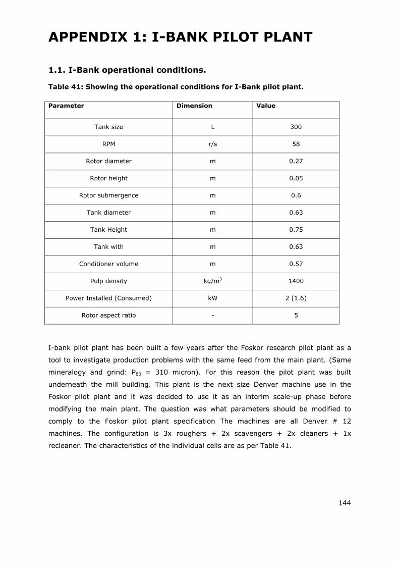
144
APPENDIX 1: I-BANK PILOT PLANT
1.1. I-Bank operational conditions.
Table 41: Showing the operational conditions for I-Bank pilot plant.
Parameter Dimension Value
Tank size L 300
RPM r/s 58
Rotor diameter m 0.27
Rotor height m 0.05
Rotor submergence m 0.6
Tank diameter m 0.63
Tank Height m 0.75
Tank with m 0.63
Conditioner volume m 0.57
Pulp density kg/m3 1400
Power Installed (Consumed) kW 2 (1.6)
Rotor aspect ratio - 5
I-bank pilot plant has been built a few years after the Foskor research pilot plant as a
tool to investigate production problems with the same feed from the main plant. (Same
mineralogy and grind: P80 = 310 micron). For this reason the pilot plant was built
underneath the mill building. This plant is the next size Denver machine use in the
Foskor pilot plant and it was decided to use it as an interim scale-up phase before
modifying the main plant. The question was what parameters should be modified to
comply to the Foskor pilot plant specification The machines are all Denver # 12
machines. The configuration is 3x roughers + 2x scavengers + 2x cleaners + 1x
recleaner. The characteristics of the individual cells are as per Table 41.
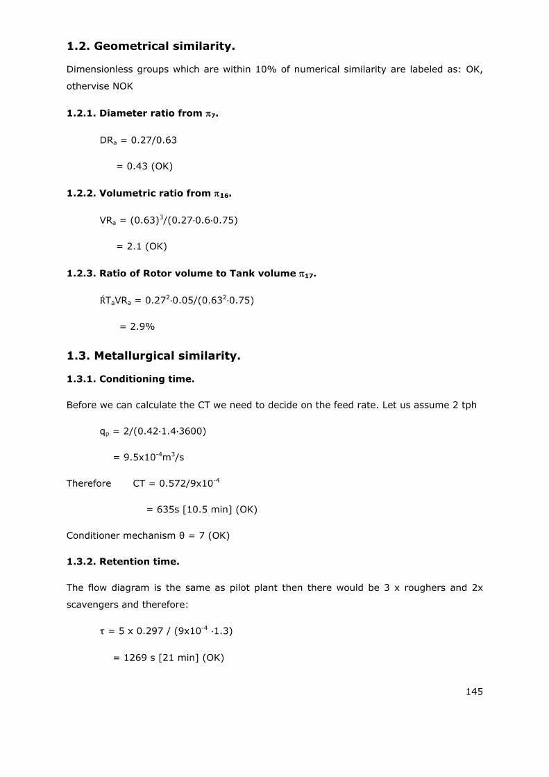
145
1.2. Geometrical similarity.
Dimensionless groups which are within 10% of numerical similarity are labeled as: OK,
othervise NOK
1.2.1. Diameter ratio from 7.
DRa = 0.27/0.63
= 0.43 (OK)
1.2.2. Volumetric ratio from 16.
VRa = (0.63)3/(0.27 0.6 0.75)
= 2.1 (OK)
1.2.3. Ratio of Rotor volume to Tank volume 17.
ŔTaVRa = 0.272 0.05/(0.632 0.75)
= 2.9%
1.3. Metallurgical similarity.
1.3.1. Conditioning time.
Before we can calculate the CT we need to decide on the feed rate. Let us assume 2 tph
qp = 2/(0.42 1.4 3600)
= 9.5x10⁻⁴m3/s
Therefore CT = 0.572/9x10-4
= 635s [10.5 min] (OK)
Conditioner mechanism θ = 7 (OK)
1.3.2. Retention time.
The flow diagram is the same as pilot plant then there would be 3 x roughers and 2x
scavengers and therefore:
τ = 5 x 0.297 / (9x10⁻⁴ 1.3)
= 1269 s [21 min] (OK)

146
(The factor = 1.3 allows for circulating load)
1.4. Hydrodynamic similarity.
1.4.1. Rotor tip Reynolds number.
Rotor tip velocity = 58 0.27/2
= 7.8m/s
Therefore Ret = 1400 7.8 0.27/1.8x10-3
= 1.7x10⁶ (OK)
1.4.2. Aeration number.
Qa = 6x10⁻³/[58 (0.63)3}
= 4.8x10⁻⁴ (NOK)
1.4.3. Circulation and relative circulation.
No info available
1.4.4. Froude number.
FrD = ω2 d2 /4 g D
= 9.9 (NOK)
1.4.5. Bubble surface area flux (Gorain model).
From Equation 56 the bubble surface area flux is equal to 31 s-1 (OK)
1.4.6. Volumetric flow.
VfN = 9x10⁻⁴ 1.3/[58 (0.63}3]
= 8x10⁻⁵ (OK)
1.4.7. Power number.
ŔPNo = 1600/1400 583 0.275
= 4.3x10⁻³ (OK)
TaPNo. = 1700/(1400 583 0.635)
= 6.3x10⁻⁵ (OK)
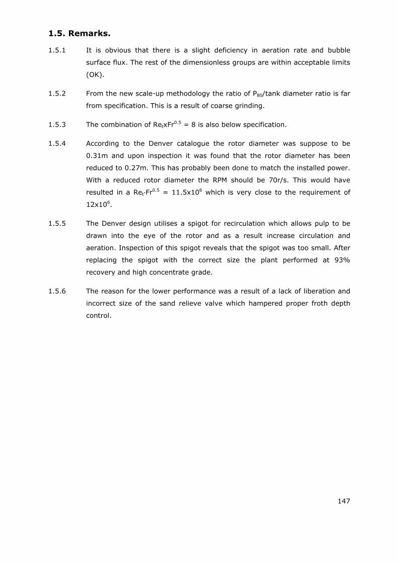
147
1.5. Remarks.
1.5.1 It is obvious that there is a slight deficiency in aeration rate and bubble
surface flux. The rest of the dimensionless groups are within acceptable limits
(OK).
1.5.2 From the new scale-up methodology the ratio of P80/tank diameter ratio is far
from specification. This is a result of coarse grinding.
1.5.3 The combination of RetxFr0.5 = 8 is also below specification.
1.5.4 According to the Denver catalogue the rotor diameter was suppose to be
0.31m and upon inspection it was found that the rotor diameter has been
reduced to 0.27m. This has probably been done to match the installed power.
With a reduced rotor diameter the RPM should be 70r/s. This would have
resulted in a Ret Fr0.5 = 11.5x10⁶ which is very close to the requirement of
12x106.
1.5.5 The Denver design utilises a spigot for recirculation which allows pulp to be
drawn into the eye of the rotor and as a result increase circulation and
aeration. Inspection of this spigot reveals that the spigot was too small. After
replacing the spigot with the correct size the plant performed at 93%
recovery and high concentrate grade.
1.5.6 The reason for the lower performance was a result of a lack of liberation and
incorrect size of the sand relieve valve which hampered proper froth depth
control.
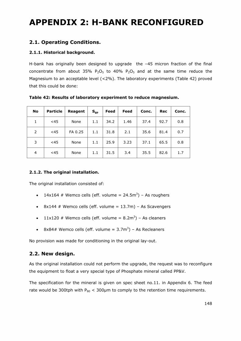
148
APPENDIX 2: H-BANK RECONFIGURED
2.1. Operating Conditions.
2.1.1. Historical background.
H-bank has originally been designed to upgrade the –45 micron fraction of the final
concentrate from about 35% P2O5 to 40% P2O5 and at the same time reduce the
Magnesium to an acceptable level (<2%). The laboratory experiments (Table 42) proved
that this could be done:
Table 42: Results of laboratory experiment to reduce magnesium.
No Particle Reagent Sgp Feed Feed Conc. Rec Conc.
1 <45 None 1.1 34.2 1.46 37.4 92.7 0.8
2 <45 FA 0.25 1.1 31.8 2.1 35.6 81.4 0.7
3 <45 None 1.1 25.9 3.23 37.1 65.5 0.8
4 <45 None 1.1 31.5 3.4 35.5 82.6 1.7
2.1.2. The original installation.
The original installation consisted of:
14x164 # Wemco cells (eff. volume = 24.5m3) – As roughers
8x144 # Wemco cells (eff. volume = 13.7m) – As Scavengers
11x120 # Wemco cells (eff. volume = 8.2m3) – As cleaners
8x84# Wemco cells (eff. volume = 3.7m3) – As Recleaners
No provision was made for conditioning in the original lay-out.
2.2. New design.
As the original installation could not perform the upgrade, the request was to reconfigure
the equipment to float a very special type of Phosphate mineral called PP&V.
The specification for the mineral is given on spec sheet no.11. in Appendix 6. The feed
rate would be 300tph with P80 < 300µm to comply to the retention time requirements.
149
2.2.1. Conditioner volume.
Conditioner volume = CoT qp
= 10 60 0.142
= 85m3
2.2.2. Rougher & Scavenger volume.
(Ro & Sc) volume = T qp 1.5 (50% circulating load)
= 22 60 0.142 1.5
= 281m3
2.2.3. Scavenger volume.
Sc volume = 0.4 281
= 112m3
Then rougher volume = 169m3.
2.2.4. Cleaner & Recleaner volume required.
(Cl & RCL) volume = 0.6 (Ro & Sc ) volume
= 0.6 281
= 168m3
2.2.5. Recleaner volume.
Recleaner volume = 0.4 (Cl & RCL) volume
= 0.4 168
= 67m3
Then available cleaner volume = 101m3
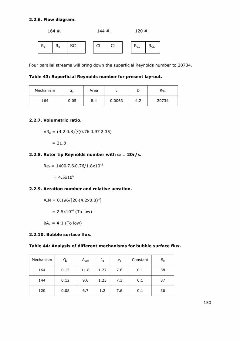
150
2.2.6. Flow diagram.
164 #. 144 #. 120 #.
Four parallel streams will bring down the superficial Reynolds number to 20734.
Table 43: Superficial Reynolds number for present lay-out.
Mechanism qp. Area v D Res
164 0.05 8.4 0.0063 4.2 20734
2.2.7. Volumetric ratio.
VRa = (4.2 0.8)3/(0.76 0.97 2.35)
= 21.8
2.2.8. Rotor tip Reynolds number with ω = 20r/s.
Ret = 1400 7.6 0.76/1.8x10-3
= 4.5x10⁶
2.2.9. Aeration number and relative aeration.
AeN = 0.196/[20 (4.2x0.8)3]
= 2.5x10⁻⁴ (To low)
ŘAe = 4:1 (To low)
2.2.10. Bubble surface flux.
Table 44: Analysis of different mechanisms for bubble surface flux.
Mechanism Qa Acell Jg vt Constant Sb
164 0.15 11.8 1.27 7.6 0.1 38
144 0.12 9.6 1.25 7.3 0.1 37
120 0.08 6.7 1.2 7.6 0.1 36
Ro Ro SC Cl Cl RCL RCL
151
The constant in this case = (ÅRa)-0.019x (P80)-0.4 = 0.102
2.2.11. Circulation and relative circulation and volumetric flow.
qc = 0.79/[20(4.2 0.85)3]
= 8.7x10⁻⁴
Rcirc = 15:1
VfN = 0.053/20(4.2)3
= 5.8x10⁻⁵
2.2.12. Power number.
ŔPNo = 48x103/[1400 (20)3 (0.76)5]
= 17x10-3
TaPNo = 7x10⁻⁶
2.3. Remarks.
The aim of the exercise was to utilise the existing equipment to the best possible extent
and therefore it is expected that there will be some shortcomings:
2.3.1. The Scavenger volume is only 50% of the rougher volume but maybe this
deficiency will be offset by the slight increase in retention time.
2.3.2. Volumetric ratio is typical of the Wemco design.
2.3.3. Superficial Reynolds number is higher than the specification but it is significantly
lower than the main plant.
2.3.4. Aeration rate, relative aeration and bubble surface area flux are below
specification. The key here is to improve P80 as all the other parameters are
fixed.
2.3.5. Volumetric flow is acceptable.
2.3.6. Power is insufficient.
152
2.4. Result.
2.4.1. This modification was never implemented but the plant was recommissioned as is
and never performed up to standard because of the reasons mentioned in
paragraph 2.
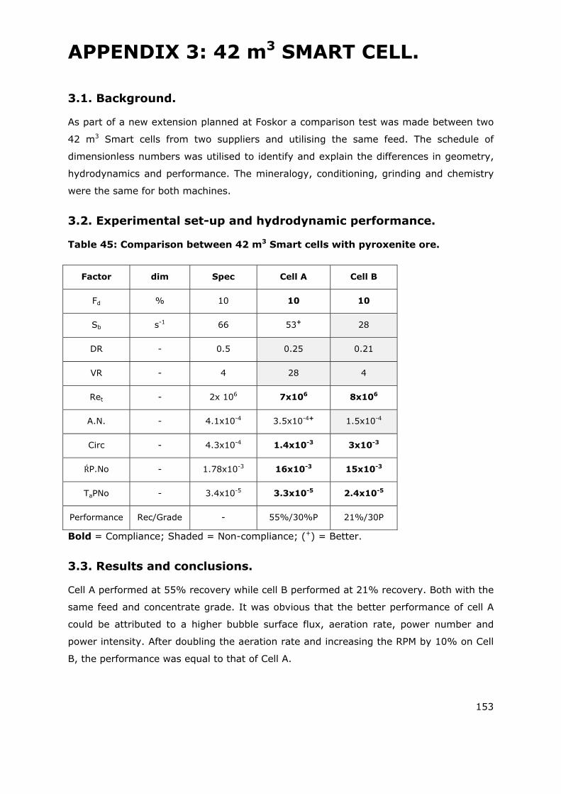
153
APPENDIX 3: 42 m3 SMART CELL.
3.1. Background.
As part of a new extension planned at Foskor a comparison test was made between two
42 m3 Smart cells from two suppliers and utilising the same feed. The schedule of
dimensionless numbers was utilised to identify and explain the differences in geometry,
hydrodynamics and performance. The mineralogy, conditioning, grinding and chemistry
were the same for both machines.
3.2. Experimental set-up and hydrodynamic performance.
Table 45: Comparison between 42 m3 Smart cells with pyroxenite ore.
Factor dim Spec Cell A Cell B
Fd % 10 10 10
Sb s-1 66 53+ 28
DR - 0.5 0.25 0.21
VR - 4 28 4
Ret - 2x 10⁶ 7x10⁶ 8x10⁶
A.N. - 4.1x10⁻⁴ 3.5x10⁻⁴+ 1.5x10⁻⁴
Circ - 4.3x10⁻⁴ 1.4x10⁻³ 3x10⁻³
ŔP.No - 1.78x10⁻³ 16x10-3 15x10-3
TaPNo - 3.4x10⁻⁵ 3.3x10⁻⁵ 2.4x10⁻⁵
Performance Rec/Grade - 55%/30%P 21%/30P
Bold = Compliance; Shaded = Non-compliance; (+) = Better.
3.3. Results and conclusions.
Cell A performed at 55% recovery while cell B performed at 21% recovery. Both with the
same feed and concentrate grade. It was obvious that the better performance of cell A
could be attributed to a higher bubble surface flux, aeration rate, power number and
power intensity. After doubling the aeration rate and increasing the RPM by 10% on Cell
B, the performance was equal to that of Cell A.

154
APPENDIX 4: BANK 15.
4.1. Background.
According to Macros (1972), the separation zone must be protected from the
turbulence and agitation from the agitation zone, and for this reason a low volumetric
ratio is required. To accomplish this, “bank 15 experiment” has been designed to test the
sensitivity of the process to the change in agitation and quiet zone. To achieve this a
modified (shortened) Wemco #164 rotor has been installed in a #120 cell (Bank 15) and
compared with a #144 short rotor in a #120 cell (Bank 13). (See Figure 64 & 65) This
modification reduced the volumetric ratio of bank 15 to 27 and this has been compared
with the bank 13 which has been refurbished with new 144 short components and
volumetric ratio of 45. (See Table 46.)
Table 46: Performance comparison between bank 13 and bank 15.
ITEM BANK 13 BANK 15
Volumetric ratio 45 27
Average rougher conc 27.9 28.1
Feed (% P2O5) 14.2 12.1
Tails (%P2O5) 10.8 9.75
Recovery (%) 39.5 30.5
Froth depth (mm) 200 200
4.2. Machine Changes.
The disappointing performance of bank 15 as indicated in Table 45 were investigated and
the following were discovered:
Bank 15 retention time was 20% less than bank 13 because of the bigger
mechanisms.
The hood was the so called high energy hood with less open area.
No gap between disperser and draft tube.
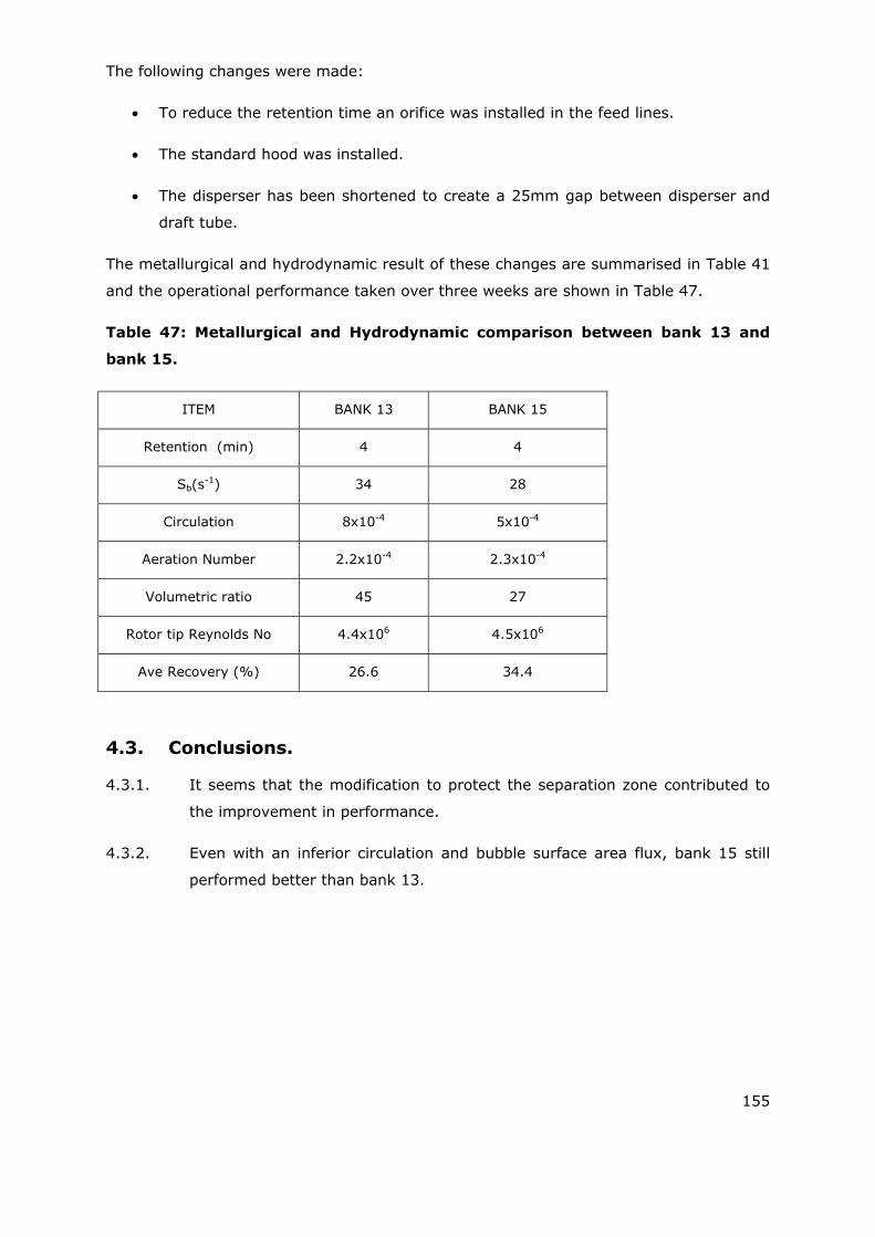
155
The following changes were made:
To reduce the retention time an orifice was installed in the feed lines.
The standard hood was installed.
The disperser has been shortened to create a 25mm gap between disperser and
draft tube.
The metallurgical and hydrodynamic result of these changes are summarised in Table 41
and the operational performance taken over three weeks are shown in Table 47.
Table 47: Metallurgical and Hydrodynamic comparison between bank 13 and
bank 15.
ITEM BANK 13 BANK 15
Retention (min) 4 4
Sb(s-1) 34 28
Circulation 8x10⁻⁴ 5x10⁻⁴
Aeration Number 2.2x10⁻⁴ 2.3x10⁻⁴
Volumetric ratio 45 27
Rotor tip Reynolds No 4.4x10⁶ 4.5x10⁶
Ave Recovery (%) 26.6 34.4
4.3. Conclusions.
4.3.1. It seems that the modification to protect the separation zone contributed to
the improvement in performance.
4.3.2. Even with an inferior circulation and bubble surface area flux, bank 15 still
performed better than bank 13.
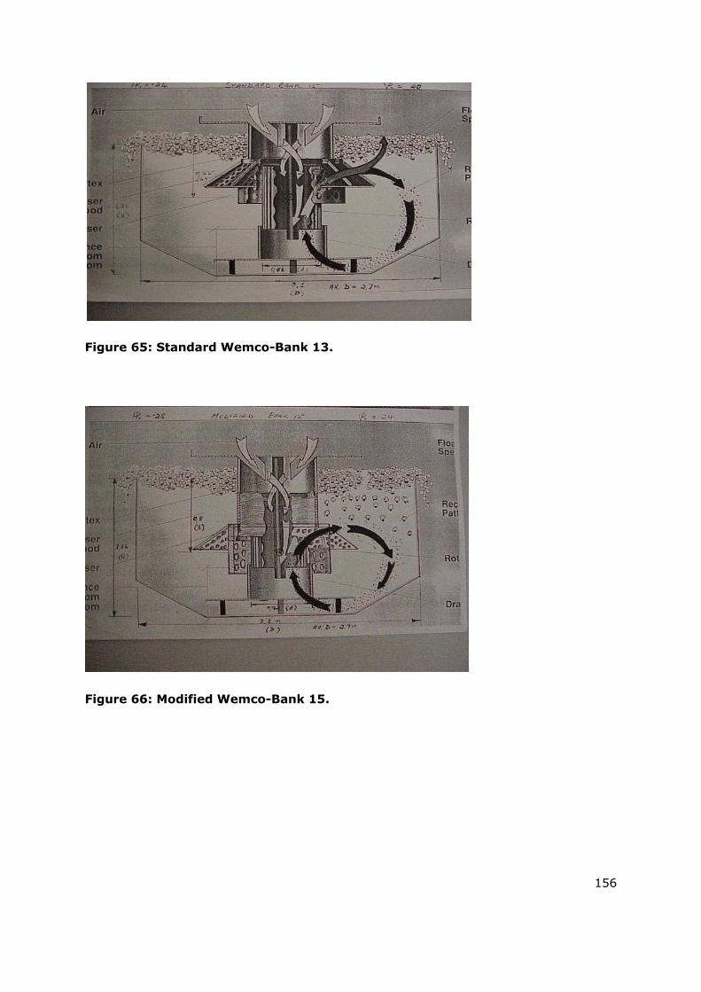
156
Figure 65: Standard Wemco-Bank 13.
Figure 66: Modified Wemco-Bank 15.
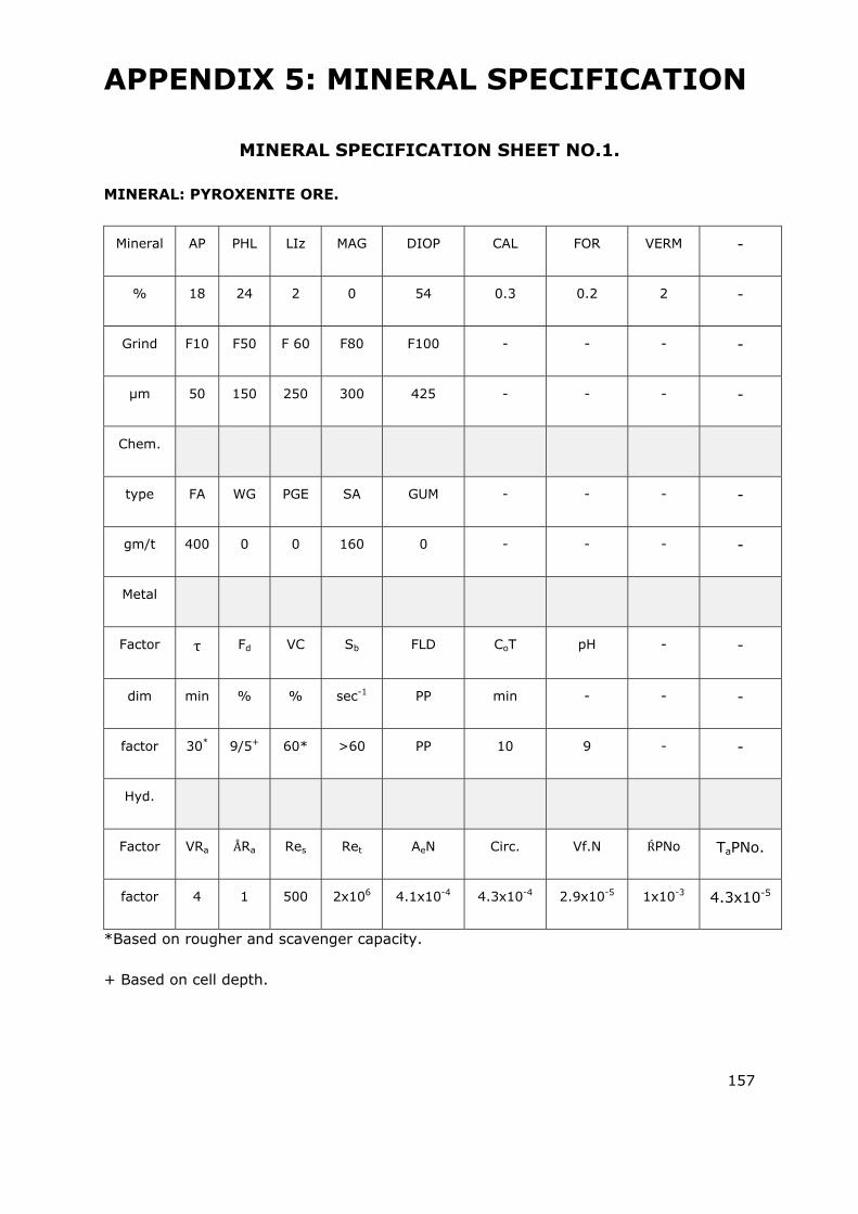
157
APPENDIX 5: MINERAL SPECIFICATION
MINERAL SPECIFICATION SHEET NO.1.
MINERAL: PYROXENITE ORE.
Mineral AP PHL LIz MAG DIOP CAL FOR VERM -
% 18 24 2 0 54 0.3 0.2 2 -
Grind F10 F50 F 60 F80 F100 - - - -
μm 50 150 250 300 425 - - - -
Chem.
type FA WG PGE SA GUM - - - -
gm/t 400 0 0 160 0 - - - -
Metal
Factor τ Fd VC Sb FLD CoT pH - -
dim min % % sec-1 PP min - - -
factor 30* 9/5+ 60* >60 PP 10 9 - -
Hyd.
Factor VRa ÅRa Res Ret AeN Circ. Vf.N ŔPNo TaPNo.
factor 4 1 500 2x10⁶ 4.1x10⁻⁴ 4.3x10⁻⁴ 2.9x10⁻⁵ 1x10⁻³ 4.3x10⁻⁵
*Based on rougher and scavenger capacity.
+ Based on cell depth.

158
MINERAL SPECIFICATION SHEET NO.2.
Mineral: FOSKORITE-CARBONATITE ORE.
Mineral AP FL LIS DIOP KAL DOL FOR FOR -
% 16 10 7 5 42 14 4 4 -
Grind F10 F50 F60 F80 F100 - - - --
μm 50 150 250 300 425 - - - -
Chem.
type FA WG PGE SA GUM - - - -
gm/t 204 347 164 >60 - - - -
Met
type τ Fd VC Sb FLD CoT pH - -
dim min % % sec-1 PP min - - -
factor 25* 9/5+ 12* >60 PP 10 9 - -
Hyd
type VRa ÅRa Res Ret AeN Circ VfN ŔPNo TaPNo
factor 4 1 500 2x10⁶ 4.1x10⁻⁴ >4.3x10⁻⁴ 2.9x10⁻⁴ 1x10⁻³ 4.3x10⁻⁵
*Based on rougher and scavenger capacity.
+ Based on cell depth.
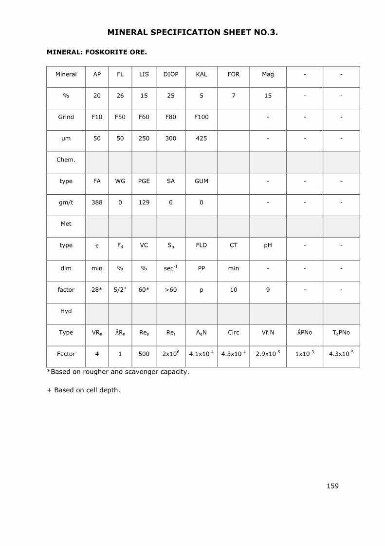
159
MINERAL SPECIFICATION SHEET NO.3.
MINERAL: FOSKORITE ORE.
Mineral AP FL LIS DIOP KAL FOR Mag - -
% 20 26 15 25 5 7 15 - -
Grind F10 F50 F60 F80 F100 - - -
μm 50 50 250 300 425 - - -
Chem.
type FA WG PGE SA GUM - - -
gm/t 388 0 129 0 0 - - -
Met
type τ Fd VC Sb FLD CT pH - -
dim min % % sec-1 PP min - - -
factor 28* 5/2+ 60* >60 p 10 9 - -
Hyd
Type VRa ÅRa Res Ret AeN Circ Vf.N ŔPNo TaPNo
Factor 4 1 500 2x10⁶ 4.1x10⁻⁴ 4.3x10⁻⁴ 2.9x10⁻⁵ 1x10⁻³ 4.3x10⁻⁵
*Based on rougher and scavenger capacity.
+ Based on cell depth.
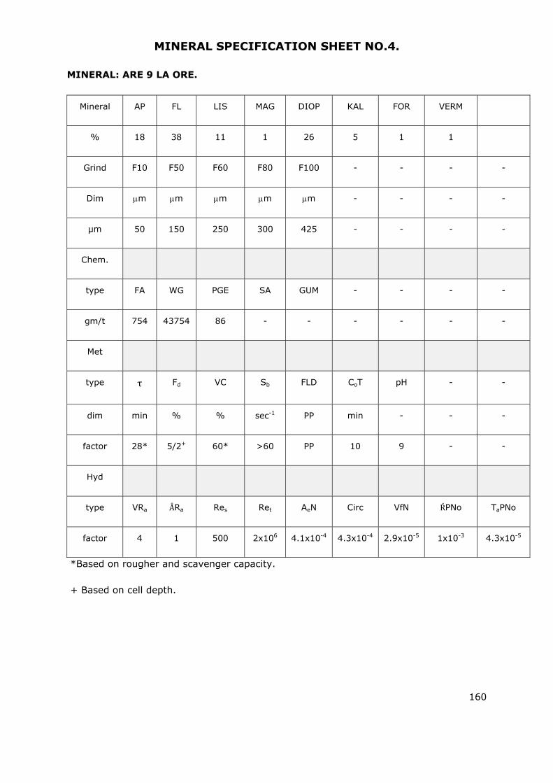
160
MINERAL SPECIFICATION SHEET NO.4.
MINERAL: ARE 9 LA ORE.
Mineral AP FL LIS MAG DIOP KAL FOR VERM
% 18 38 11 1 26 5 1 1
Grind F10 F50 F60 F80 F100 - - - -
Dim m m m m m - - - -
μm 50 150 250 300 425 - - - -
Chem.
type FA WG PGE SA GUM - - - -
gm/t 754 43754 86 - - - - - -
Met
type τ Fd VC Sb FLD CoT pH - -
dim min % % sec-1 PP min - - -
factor 28* 5/2+ 60* >60 PP 10 9 - -
Hyd
type VRa ÅRa Res Ret AeN Circ VfN ŔPNo TaPNo
factor 4 1 500 2x10⁶ 4.1x10⁻⁴ 4.3x10⁻⁴ 2.9x10⁻⁵ 1x10⁻³ 4.3x10⁻⁵
*Based on rougher and scavenger capacity.
+ Based on cell depth.
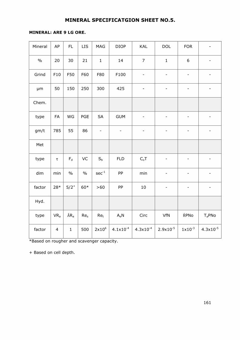
161
MINERAL SPECIFICATGION SHEET NO.5.
MINERAL: ARE 9 LG ORE.
Mineral AP FL LIS MAG DIOP KAL DOL FOR -
% 20 30 21 1 14 7 1 6 -
Grind F10 F50 F60 F80 F100 - - - -
μm 50 150 250 300 425 - - - -
Chem.
type FA WG PGE SA GUM - - - -
gm/t 785 55 86 - - - - - -
Met
type τ Fd VC Sb FLD CoT - - -
dim min % % sec-1 PP min - - -
factor 28* 5/2+ 60* >60 PP 10 - - -
Hyd.
type VRa ÅRa Res Ret AeN Circ VfN ŔPNo TaPNo
factor 4 1 500 2x10⁶ 4.1x10⁻⁴ 4.3x10⁻⁴ 2.9x10⁻⁵ 1x10⁻³ 4.3x10⁻⁵
*Based on rougher and scavenger capacity.
+ Based on cell depth.
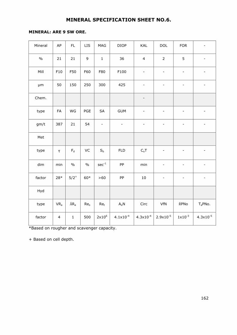
162
MINERAL SPECIFICATION SHEET NO.6.
MINERAL: ARE 9 SW ORE.
Mineral AP FL LIS MAG DIOP KAL DOL FOR -
% 21 21 9 1 36 4 2 5 -
Mill F10 F50 F60 F80 F100 - - - -
μm 50 150 250 300 425 - - - -
Chem. -
type FA WG PGE SA GUM - - - -
gm/t 387 21 54 - - - - - -
Met
type τ Fd VC Sb FLD CoT - - -
dim min % % sec-1 PP min - - -
factor 28* 5/2+ 60* >60 PP 10 - - -
Hyd
type VRa ÅRa Res Ret AeN Circ VfN ŔPNo TaPNo.
factor 4 1 500 2x10⁶ 4.1x10⁻⁴ 4.3x10⁻⁴ 2.9x10⁻⁵ 1x10⁻³ 4.3x10⁻⁵
*Based on rougher and scavenger capacity.
+ Based on cell depth.

163
MINERAL SPECIFICATION SHEET NO.7.
MINERAL: ARE 9 F11A ORE.
Mineral AP FL LIS MAG DIOP KAL DOL FOR -
% 18 40 11 1 17 4 2 6 -
Grind F10 F50 F60 F80 F100 - - - -
μm 50 150 250 300 425 - - - -
Chem.
Type FA WG PGE SA GUM - - - -
gm/t 672 43 129 - - - - - -
Met
Type τ Fd VC Sb FLD CoT pH - -
Dim min % % sec-1 PP min - - -
factor 28* 5/2+ 60* >60 PP 10 9 - -
Hyd
type VRa ÅRa Res Ret AeN Circ VfN ŔPNo TaPNo
factor 4 1 500 2x10⁶ 4.1x10⁻⁴ 4.3x10⁻⁴ 2.9x10⁻⁵ 1x10⁻³ 4.3x10⁻⁵
*Based on rougher and scavenger capacity.
+ Based on cell depth.
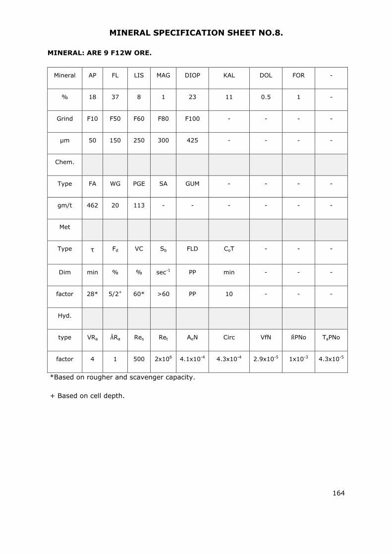
164
MINERAL SPECIFICATION SHEET NO.8.
MINERAL: ARE 9 F12W ORE.
Mineral AP FL LIS MAG DIOP KAL DOL FOR -
% 18 37 8 1 23 11 0.5 1 -
Grind F10 F50 F60 F80 F100 - - - -
μm 50 150 250 300 425 - - - -
Chem.
Type FA WG PGE SA GUM - - - -
gm/t 462 20 113 - - - - - -
Met
Type τ Fd VC Sb FLD CoT - - -
Dim min % % sec-1 PP min - - -
factor 28* 5/2+ 60* >60 PP 10 - - -
Hyd.
type VRa ÅRa Res Ret AeN Circ VfN ŔPNo TaPNo
factor 4 1 500 2x10⁶ 4.1x10⁻⁴ 4.3x10⁻⁴ 2.9x10⁻⁵ 1x10⁻³ 4.3x10⁻⁵
*Based on rougher and scavenger capacity.
+ Based on cell depth.
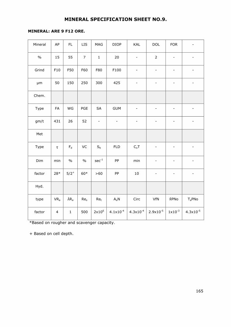
165
MINERAL SPECIFICATION SHEET NO.9.
MINERAL: ARE 9 F12 ORE.
Mineral AP FL LIS MAG DIOP KAL DOL FOR -
% 15 55 7 1 20 - 2 - -
Grind F10 F50 F60 F80 F100 - - - -
μm 50 150 250 300 425 - - - -
Chem.
Type FA WG PGE SA GUM - - - -
gm/t 431 26 52 - - - - - -
Met
Type τ Fd VC Sb FLD CoT - - -
Dim min % % sec-1 PP min - - -
factor 28* 5/2+ 60* >60 PP 10 - - -
Hyd.
type VRa ÅRa Res Ret AeN Circ VfN ŔPNo TaPNo
factor 4 1 500 2x10⁶ 4.1x10⁻⁴ 4.3x10⁻⁴ 2.9x10⁻⁵ 1x10⁻³ 4.3x10⁻⁵
*Based on rougher and scavenger capacity.
+ Based on cell depth.

166
MINERAL SPECIFICATION SHEET NO.10.
MINERAL: PMM TAIL DAM ORE.
Mineral AP FL LIS MAG DIOP KAL DOL FOR -
% 20 8 15 3 5 20 - - -
Grind F10 F50 F60 F80 F100 - - - -
μm 10 105 150 300 500 - - - -
Chem.
Type FA WG PGE SA GUM - - - -
gm/t 388 350 150 0 60 - - - -
Met
Type τ Fd VC Sb FLD CoT pH - -
Dim min % % sec-1 PP Min - - -
factor 25* 9/5+ 60* >60 PP 10 9 - -
Hyd
type VRa ÅRa Res Ret AeN Circ VfN ŔPNo TaPNo
factor 4 1 500 2x10⁶ 4.1x10⁻⁴ 4.3x10⁻⁴ 2.9x10⁻⁵ 1x10⁻³ 4.3x10⁵
*Based on rougher and scavenger capacity.
+ Based on cell depth.
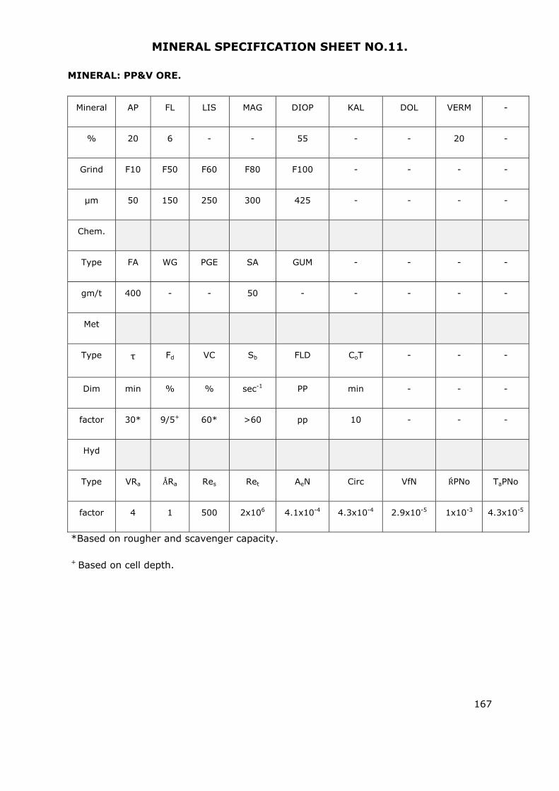
167
MINERAL SPECIFICATION SHEET NO.11.
MINERAL: PP&V ORE.
Mineral AP FL LIS MAG DIOP KAL DOL VERM -
% 20 6 - - 55 - - 20 -
Grind F10 F50 F60 F80 F100 - - - -
μm 50 150 250 300 425 - - - -
Chem.
Type FA WG PGE SA GUM - - - -
gm/t 400 - - 50 - - - - -
Met
Type τ Fd VC Sb FLD CoT - - -
Dim min % % sec-1 PP min - - -
factor 30* 9/5+ 60* >60 pp 10 - - -
Hyd
Type VRa ÅRa Res Ret AeN Circ VfN ŔPNo TaPNo
factor 4 1 500 2x10⁶ 4.1x10⁻⁴ 4.3x10⁻⁴ 2.9x10⁻⁵ 1x10⁻³ 4.3x10⁻⁵
*Based on rougher and scavenger capacity.
+ Based on cell depth.
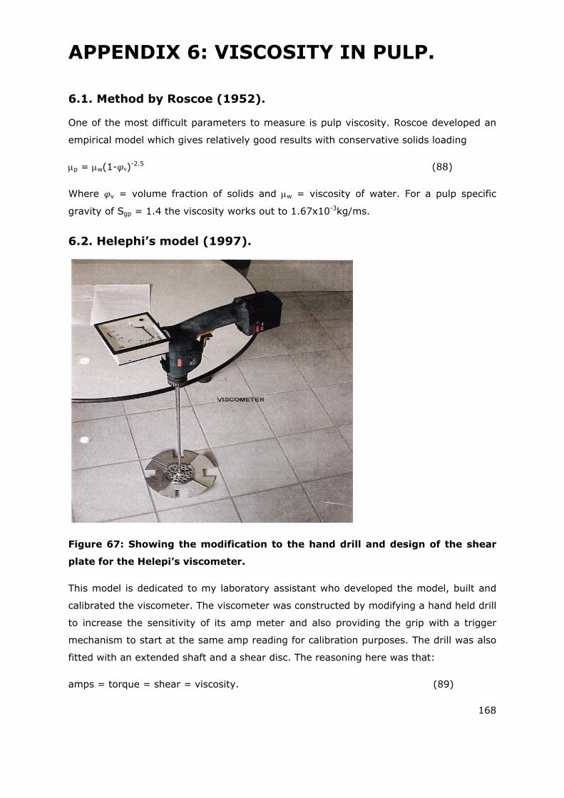
168
APPENDIX 6: VISCOSITY IN PULP.
6.1. Method by Roscoe (1952).
One of the most difficult parameters to measure is pulp viscosity. Roscoe developed an
empirical model which gives relatively good results with conservative solids loading
p = w(1- v)-2.5 (88)
Where v = volume fraction of solids and w = viscosity of water. For a pulp specific
gravity of Sgp = 1.4 the viscosity works out to 1.67x10⁻³kg/ms.
6.2. Helephi’s model (1997).
Figure 67: Showing the modification to the hand drill and design of the shear
plate for the Helepi’s viscometer.
This model is dedicated to my laboratory assistant who developed the model, built and
calibrated the viscometer. The viscometer was constructed by modifying a hand held drill
to increase the sensitivity of its amp meter and also providing the grip with a trigger
mechanism to start at the same amp reading for calibration purposes. The drill was also
fitted with an extended shaft and a shear disc. The reasoning here was that:
amps = torque = shear = viscosity. (89)
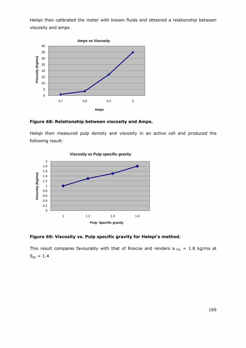
169
Helepi then calibrated the meter with known fluids and obtained a relationship between
viscosity and amps.
Figure 68: Relationship between viscosity and Amps.
Helepi then measured pulp density and viscosity in an active cell and produced the
following result:
Figure 69: Viscosity vs. Pulp specific gravity for Helepi’s method.
This result compares favourably with that of Roscoe and renders a p = 1.8 kg/ms at
Sgp = 1.4
0
5
10
15
20
25
30
35
40
3.7 3.8 4.2 5
Vis
cosi
ty (
Kg
/ms)
Amps
Amps vs Viscosity
0
0.2
0.4
0.6
0.8
1
1.2
1.4
1.6
1.8
2
1 1.2 1.3 1.4
Vis
cosi
ty (
Kg
/ms)
Pulp Specific gravity
Viscosity vs Pulp specific gravity
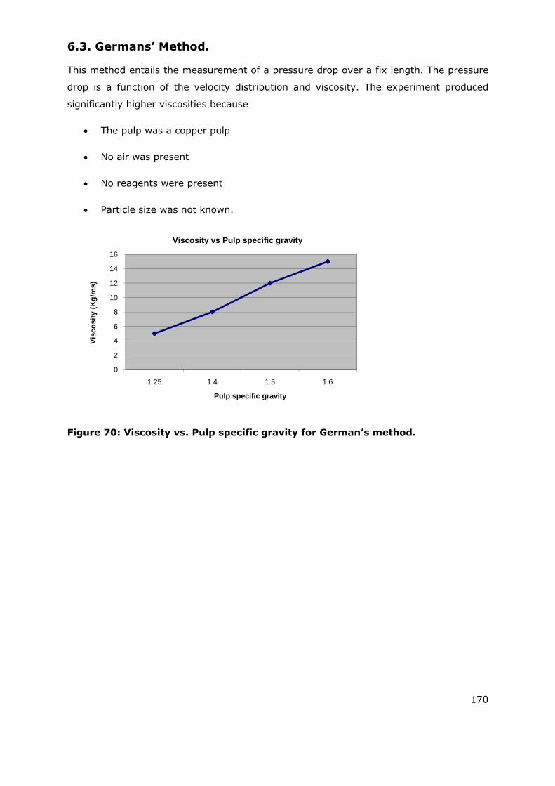
170
6.3. Germans’ Method.
This method entails the measurement of a pressure drop over a fix length. The pressure
drop is a function of the velocity distribution and viscosity. The experiment produced
significantly higher viscosities because
The pulp was a copper pulp
No air was present
No reagents were present
Particle size was not known.
Figure 70: Viscosity vs. Pulp specific gravity for German’s method.
0
2
4
6
8
10
12
14
16
1.25 1.4 1.5 1.6
Vis
cosi
ty (
Kg
/ms)
Pulp specific gravity
Viscosity vs Pulp specific gravity
171
APPENDIX 7: DETAIL DIMENSIONLESS ANALYSIS.
7.1. Variables.
Table 6 contains the relevant list for a mechanically agitated flotation process. The
technique chosen for dimensional analysis is the method of repeating variables. In this
case three repeating variables are chosen (Because three dimensions exist) and a fourth
one is added to form a dimensionless group by equating the function to one. ( ‐group .
The choice of repeating variables are:
Pulp density = ρp (ML-3)
Some linear velocity = v (LT-2)
Tank diameter = D (L)
7.2. Developing of π-groups.
7.2.1. Geometrical groups.
7.2.1.1.Rotor diameter: d (m) - π1
ρpx vy Dz d =1 (89)
Replace variables with dimensions and equate to zero:
[ML-3]x [LT-1]y [L]Z [L] =0
Compare exponents for each dimension:
M: x = 0
L: y +z +1 = 0 y + z = -1
172
T: -y = 0
X = 0 : y = 0 : z = -1
Substitute in (89):
π1 = d/D (Diameter ratio).
When rotor diameter is replaced with any other linear variable then it will result in a
similar group as π1.
7.2.1.2. Geometrical dimensionless groups
1 = Diameter ratio (DRa) = d/D
2 = Relative particle size (Řps) = P80/D
3 = Tank slenderness ratio (TaSRa) = H/D
4 = Relative froth depth (ŘFd) = Fd/D
5 = Submergence ratio (Su) = h /D
6 = Rotor height (Rh) = e/D
7.2.2. Kinematic groups.
7.2.2.1. Aeration: qa (m3/s) - 7 and circulation: qc (m3/s) - 8
ρpx vy Dz qa =1 (90)
Replace variables with dimensions and equate to zero:
[ML-3]x [LT-1]y [L]Z [L3T-1] =0
Compare exponents for each dimension:
M: x = 0
173
L: y +z +3 = 0 y + z = -3
T: -y -1 = 0 y = -1
X = 0 : y = -1 : z = -2
Substitute in (90)
7 = qa /vD2
When v is replaced by ωD then equation becomes:
7 = qa /ωD3 (Aeration number)
The same applies to the circulation requirement:
8 = qc /ωD3 (Circulation number)
7.2.2.2. Conditioning time η (s) -9 , froth retention time ξ s ‐-10 and Conditioner Tank
turn Around θ s‐1
ρpx vy Dz η =1 (91)
Replace variables with dimensions and equate to zero:
[ML-3]x [LT-1]y [L]Z [T] =0
Compare exponents for each dimension:
M: x = 0
L: y +z = 0 y = -z
T: -y +1 = 0 y = 1
X = 0 : y = 1 : z = -1
174
9 = vη/D
Replace v with ωD
9 = ωη ( Dimensionless conditioning time)
The same manipulation for ξ and θ:
10 θ/ω Dimensionless Tank turn around
11 = ωξ (Dimensionless froth retention time)
7.2.2.3. Viscosity μ (kg/ms) - π12 and gravity g (m/s2) - π13
ρpx vy Dz μ =1 (92)
Replace variables with dimensions and equate to zero:
[ML-3]x [LT-1]y [L]Z [ML-1T-1] =0
Compare exponents for each dimension:
M: x + 1 = 0 x = -1
L: -3x +y +z -1 = 0 y + z = -2
T: -y -1 = 0 y = -1
X = -1 : y = -1 : z = -1
Replace in equation (92)
π12 µ/ρp v D
or
175
π12 ρp v D/µ (Superficial Reynolds number)
When µ is replaced by gravity then:
ρpx vy Dz g =1 (93)
Replace variables with dimensions and equate to zero:
[ML-3]x [LT-1]y [L]Z [LT-2] =0
Compare exponents for each dimension:
M: x = 0
L: y +z +1 = 0 y + z = -1
T: -y -2 = 0 y = -2
X = 0 : y = -2 : z = 1
Replace in equation (93)
π13 gD/v2
Replace v with ωd and invert, then π13 becomes
π13 ω2d2/gD Froude number based on tank diameter
7.2.2.4. Kinematic dimensionless groups
7 = Aeration number (AeN) = q/.D3
8 = Circulation number (CN) = Qc/.D3
9 = Dimensionless Conditioning time (CoT) = ω
9 = Conditioner tank turn around (θ) = θ/ω
11 = Dimensionless Froth retention time (FRT) = ω.ξ

176
12 = Superficial Reynolds number (Res) = ρp.ω.D2/µp
13 = Froude No (Fr) = ω2D/g
7.2.3. Dynamic groups.
7.2.3.1. Absorbed power P (kW) - 14
ρpx vy Dz P =1 (94)
Replace variables with dimensions and equate to zero:
[ML-3]x [LT-1]y [L]Z [ML2T-3] =0
Compare exponents for each dimension:
M: x + 1= 0 x=-1
L: -3x + y +z +2 = 0 y + z = -5
T: -y -3 = 0 y = -3
X = -1 : y = -3 : z =-2
Replace in equation (94)
π14 ρ‐1 v‐3 D ‐2 P
Replace v with ωD and invert, then π14 becomes:
π14 P/ ρ ω3 D5 Tank power number
7.2.3.2. Surface tension σ ( N/m) - π15
ρpx vy Dz σ =1 (95)
Replace variables with dimensions and equate to zero:
177
[ML-3]x [LT-1]y [L]Z [MT-2] =0
Compare exponents for each dimension:
M: x + 1= 0 x=-1
L: -3x + y +z = 0 y + z = -3
T: -y -2 = 0 y = -2
X = -1 : y = -2 : z = -1
Replace in equation (95)
π15 ρ‐1 v‐2 D‐1 σ
Replace v with ωD and invert, then π15 becomes:
π15 ρ ω2 D3 / σ Weber number
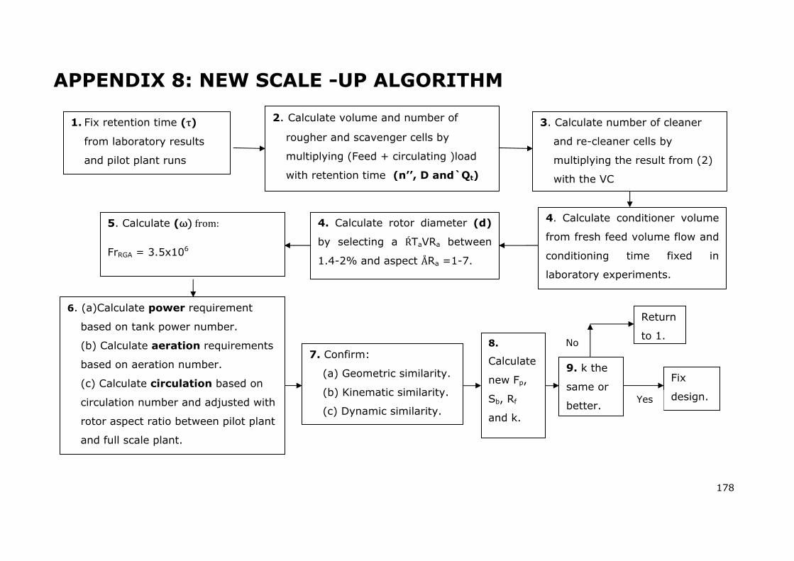
178
APPENDIX 8: NEW SCALE -UP ALGORITHM
1. Fix retention time (τ)
from laboratory results
and pilot plant runs
2. Calculate volume and number of
rougher and scavenger cells by
multiplying (Feed + circulating )load
with retention time (n’’, D and`Qt)
3. Calculate number of cleaner
and re-cleaner cells by
multiplying the result from (2)
with the VC
4. Calculate rotor diameter (d)
by selecting a ŔTaVRa between
1.4-2% and aspect ÅRa =1-7.
5. Calculate (ω from:
FrRGA = 3.5x10⁶
6. (a)Calculate power requirement
based on tank power number.
(b) Calculate aeration requirements
based on aeration number.
(c) Calculate circulation based on
circulation number and adjusted with
rotor aspect ratio between pilot plant
and full scale plant.
7. Confirm:
(a) Geometric similarity.
(b) Kinematic similarity.
(c) Dynamic similarity.
8.
Calculate
new Fp,
Sb, Rf
and k.
4. Calculate conditioner volume
from fresh feed volume flow and
conditioning time fixed in
laboratory experiments.
9. k the
same or
better.
Fix
design. Yes
Return
to 1. No