saurashtra universityetheses.saurashtrauniversity.edu/916/1/gilani_ms_thesis_statistics.pdfdoctor of...

Saurashtra University Re – Accredited Grade ‘B’ by NAAC (CGPA 2.93)

Gaglani, Mansi S., 2011, “A study on Transportation Problem, Transshipment Problem, Assignment Problem and Supply Chain Management”, thesis PhD, Saurashtra University

http://etheses.saurashtrauniversity.edu/id/916 Copyright and moral rights for this thesis are retained by the author A copy can be downloaded for personal non-commercial research or study, without prior permission or charge. This thesis cannot be reproduced or quoted extensively from without first obtaining permission in writing from the Author. The content must not be changed in any way or sold commercially in any format or medium without the formal permission of the Author When referring to this work, full bibliographic details including the author, title, awarding institution and date of the thesis must be given.

Saurashtra University Theses Service http://etheses.saurashtrauniversity.edu

[email protected]

© The Author

A Study on Transportation Problem, Transshipment

Problem, Assignment Problem and Supply Chain

Management

A THESIS SUBMITTED TO

DEPARTMENT OF STATISTICS, SAURASHTRA UNIVERSITY

RAJKOT-360005

FOR

THE AWARD OF THE DEGREE OF

DOCTOR OF PHILOSOPHY

IN

STATISTICS

UNDER THE FACULTY OF SCIENCE

By

Ms. Mansi Suryakant Gaglani

Research Fellow

Department of Statistics

Saurashtra University

Rajkot-360005

Under the Guidance of

Professor D. K. Ghosh

Head of Department of Statistics


Rajkot, Gujarat, India

REGISTRATION NO.: 4064 DATE: 22nd OCTOBER 2011

CERTIFICATE

This is to certify that Ms. Mansi Suryakant Gaglani has worked under my

guidance for the award of degree of Doctor of Philosophy in Statistics

(Operations Research) under Faculty of Science on the topic entitled “A Study

on Transportation Problem, Transshipment Problem, Assignment Problem

and Supply Chain Management”.

We further certify that the work has not been submitted either partially or

fully to any other University/Institute for the award of any degree.

Date: 22/10/2011 Dr. D. K. Ghosh (Guide)

Place: Rajkot Department of Statistics



Date: 22/10/2011 Dr. D. K. Ghosh

Place: Rajkot Professor and Head




DECLARATION

I hereby declare that the thesis carried out by me at the Department of

Statistics, Saurashtra University, Rajkot, Gujarat, India submitted to the Faculty

of Science, Saurashtra University, Rajkot and the work incorporated in the

present thesis is original and has not been submitted to any University/Institution

for the award of the degree.

I am hearty thankful to Dr. D. K. Ghosh who provided me his guidance

fully and allow me to submit my research paper in different journals.

Date: 22/10/2011 Ms. Mansi S. Gaglani

Place: Rajkot Research Fellow



Rajkot-360005

Gujarat, India

ACKNOWLEDGEMENT

I am very much thankful to God for giving her blessing and strength to

complete my work. Let God bless me for my future academic work. I bow before

God as I completed my the mighty task of Ph. D. Research work in the proper

time.

I would like to give my gratitude to my guide, Dr. D. K. Ghosh, Professor

and Head of the Department of Statistics, Saurashtra University, Rajkot for his

valuable guidance. I hearty pay my deepest sense of gratitude to Dr. D. K. Ghosh

who made my career in academic process through out my academic career from

Master degree to Ph.D. During my research work at the department he was

constantly guiding, advising, helping in finding the reprints and providing the

selfless encouragement in proving the results. I am debt to him for his regular

discussion about the research and his blessings. Without his inspiration, it could

not have been possible from any source of my life to complete this Ph. D.

Research work in Statistics. Today whatever academically I achieved, it is due to

my Sir Dr. D. K. Ghosh. I will be faithful to him in my whole life. It was not

possible for me to begin my research activity due to some unavoidable reasons

but because of his humble inspiration and cooperation I took the decision in order

to continue my research work. During my academic work from P.G. to Ph.D., he

neither refused nor gave me any other date whenever I approached him for

seeking guidance, any difficulty or queries related with my research work.

Whatever I expressed my thankful to him will be list for me.

I express my deepest sense of gratitude to owe my loving mother Meeta

S. Gaglani and father Suryakant G. Gaglani for their cooperations,

encouragement and blessing through out my academic career, without their help,

support and good wishes, this work could not have been completed. I am grateful

to my grandmother Jaya G. Gaglani who provides me her company and blessing

in completing this mighty task. I am really owed to my eldest brother Dhaval and

my sweetest Bhabhi Nisha. I am heartiest thankful to my younger brother Nikunj

without their help, this work could not have been completed.

I have no words to express my sincere thanks to all my colleagues and

friends especially to Falguni, Neha, Maulik and Denish without their constant

touch, inspiration, support and motivation, I could not have reach at this stage. I

am hearty thankful to all my friends who help me knowingly or unknowingly.

I am really thankful to office staff of Department of Statistics, Saurashtra

University, Rajkot for their relevant support.

Mansi

CONTENTS

Chapter No. Title

Page No.

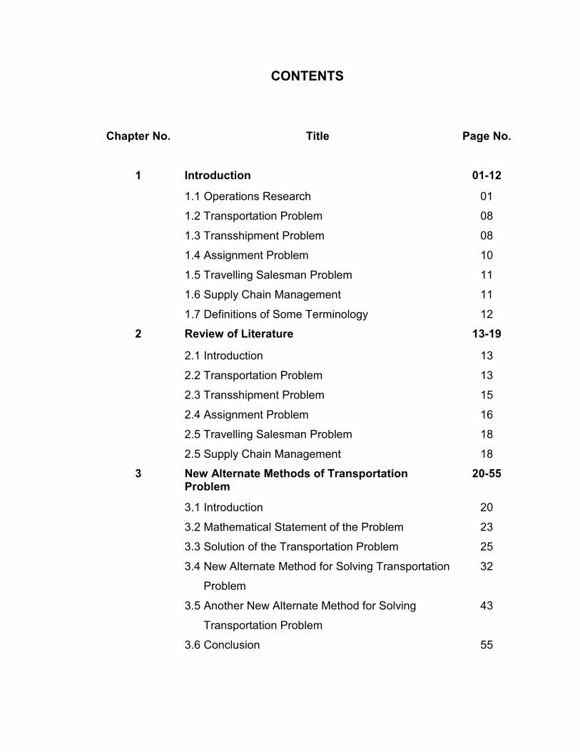
1 Introduction 01-12

1.1 Operations Research

1.2 Transportation Problem

1.3 Transshipment Problem

1.4 Assignment Problem

1.5 Travelling Salesman Problem

1.6 Supply Chain Management

1.7 Definitions of Some Terminology

01

08

08

10

11

11

12

2 Review of Literature 13-19

2.1 Introduction






13

13

15

16

18

18

3 New Alternate Methods of Transportation Problem

20-55

3.1 Introduction

3.2 Mathematical Statement of the Problem

3.3 Solution of the Transportation Problem

3.4 New Alternate Method for Solving Transportation

Problem

3.5 Another New Alternate Method for Solving

Transportation Problem

3.6 Conclusion

20

23

25

32

43

55

4 A New Alternate Method of Transshipment Problem

56-68

4.1 Introduction


4.3 Solution of the Transshipment Problem

4.4 A New Alternate Method for Solving

Transshipment Problem

4.5 Conclusion

56

58

59

62

68

5 A New Alternate Method of Assignment Problem 69-97

5.1 Introduction


5.3 Solution of the Assignment Problem

5.4 A New Alternate Method for Solving

Assignment Problem

5.5 Conclusion

69

71

73

80

97

6 Travelling Salesman Problem 98-103

6.1 Introduction

6.2 Application of New Alternate Method of AP in

TSP

6.3 Conclusion

98

99

103

7 Supply Chain Management 104-114

7.1 Introduction

7.2 Mathematical Model of SCM

7.3 Conclusion

104

110

114

8 Conclusions and Scope of Future Work 115-116

References 117-122

PAPER SUBMITTED FOR PUBLICATIONS

1. Ghosh, D. K. & Mansi, S. G. (2011). A new alternate method of

Transportation Problem, Journal of OR Insight (under review).


Transportation Problem, Journal of Sankhya Vigyan (under review).


Transshipment Problem, Journal of Opsearch (under review).


Assignment Problem, European Journal of Operations Research

(under review).

1

CHAPTER 1

INTRODUCTION

1.1 Operations Research

Operations Research, Operational Research or simply O.R. is the use of

Mathematical models, Statistics and algorithms to aid in decision-making. It is

most often used to analyze complex real-world systems, typically with the goal of

improving or optimizing performance. It is one form of the applied mathematics.

Operations Research is an interdisciplinary branch of applied mathematics and

formal science that uses methods such as mathematical modeling, statistics, and

algorithms to arrive at optimal or near optimal solutions to complex problems. It is

typically concerned with optimizing the maxima (for an example, profit, assembly

line performance, crop yield, bandwidth, etc) or minima (for an example, loss,

risk, etc.) of some objective function. Operations research helps the management

to achieve its goals using scientific methods.

As per history of Operations Research, it is claimed that Charles Babbage

(1791-1871) is the "father of operations research" because his research into the

cost of transportation and sorting of mail led to England's universal "Penny Post"

in 1840 and studies into the dynamical behavior of railway vehicles in defense of

the GWR's broad gauge. The modern field of operations research arose during

World War II. Scientists in the United Kingdom including Patrick Blackett, Cecil

Gordon, C. H. Waddington, Owen Wansbrough-Jones and Frank Yates and

George Dantzig (United States) looked for ways to make better decisions in such

areas as logistics and training schedules. After the war it began to be applied to

similar problems in industry.

2

The terms operations research and management sciences are often used

synonymously. When a distinction is drawn, management science generally

implies a closer relationship to the problems of business management. The field

is closely related to Industrial engineering, but takes more of an engineering point

of view. Industrial engineers typically consider Operations Research (OR)

techniques to be a major part of their toolset. Some of the primary tools used by

operations researchers are statistics, optimization, probability theory, queuing

theory, game theory, graph theory, decision analysis and simulation techniques.

Because of the computational nature of these fields, OR also has ties to

computer science, and hence operations researchers use custom-written and off-

the-shelf software.

Operations research is distinguished by its frequent use to examine an entire

management information system, rather than concentrating only on specific

elements (though this is often done as well). An operations researcher faced with

a new problem that is expected to determine which techniques are most

appropriate for the given nature of the system, the goals for improvement, and

constraints on time and computing power. For this and other reasons, the human

element of OR is vital. Like any other tools, OR techniques cannot solve

problems by themselves. The operations research analyst has a wide variety of

methods available for problem solving. For mathematical programming models

there are optimization techniques appropriate for almost every type of problem,

although some problems may be difficult to solve. For models that incorporate

statistical variability there are methods such as probability analysis and

simulation that estimate statistics for output parameters. In most cases the

methods are implemented in computer programs. It is important that at least

some member of an OR study team be aware of the tools available and be

knowledgeable concerning their capabilities and limitations.

Along the history, is frequent to find collaboration among scientists and

armies officer with the same objective, ruling the optimal decision in battle. In fact

that many experts considered the start of Operational Research in the III century

3

B.C. during the II Punic War with analysis and solution that Arquimedes named

for the defense of the city of Syracuse, besieged for Romans. Enter his

inventions would find the catapult, and a system of mirrors that was setting to fire

the enemy boats by focusing them with the Sun's rays.

Leornado DaVinci (1503), being an engineer took part in the war against

Prisa because he knew the techniques to accomplish bombardments, to

construct ships, armored vehicles, cannons, catapults and another warlike

machine. Another antecedent of use of Operational Research by F.W.

Lanchester, who made a mathematical study about the ballistic potency of

opponents and hence he developed from a system of equations differential and

then called it Lanchester's Square Law that can be available to determine the

outcome of a military battle. Thomas Edison made use of Operational Research

by contributing in the antisubmarine war, with his greats ideas, like shields

against torpedo for the ships. From the mathematical point of view many

mathematicians, in centuries XVII and XVIII, like Newton, Leibnitz, Bernoulli and

Lagrange etc. worked in obtaining maximum and minimum conditions of certain

functions. Mathematical French Jean Baptiste and Joseph Fourier sketched

methods of present-day Linear Programming. During later years of the century

XVIII, Gaspar Monge laid down the precedents of the Graphical Method thanks

to his development of Descriptive Geometry. Janos Von Neumann (1944)

published his work called "Theory of Games", that provided the basic concept of

Linear Programming to Mathematicians. Neumann (1947) viewed the similitude

among the linear programming problems and the matrix theory that developed by

himself. Russian mathematician Kantorovich (1939) in association with another

Dutchman mathematician Koopmans (1939) developed the mathematical theory

called "Linear programming". This investigation rewarded them with the Nobel

Prize.

In the late years 30, George Joseph Stigler presented a particular problem

known as special diet optimal or more commonly known as problem of the diet

that happened because the worry of the USA army to guarantee some

4

nutritionals requests to the lower cost for his troops. It was solved with a heuristic

method which solutions only differ in some centimes against the solution

contributed years later by the Simplex Method. During the years 1941 and 1942,

Kantorovich and Koopmans studied independently about the Transport Problem

for first time. Initially this type of problems for solving Transport Problem was

called problem of Koopmans-Kantorovich. For his solution, they used geometric

methods that are related to Minkowski's theory of convexity. But it does not

considered that has been born a new science called Operations Research until

the II World War, during battle of England, where Deutsche Air Force, that is the

Luftwaffe, was submitting the Britishers to a hard air raid, since these had an little

aerial capability, although experimented in the Combat. The British government

looking for some method to defend his country convoked several scientists of

various disciplines for try to resolve the problem to get the peak of benefit of

radars that they had. Thanks to his work for determining the optimal localization

of antennas and further they got the best distribution of signals to double the

effectiveness of the system of aerial defense. To notice the range of this new

discipline, England created another groups of the same nature in order to obtain

optimal results in the dispute. Just like United States (USA), when joined the War

in 1942, creating the project SCOOP (Scientific Computation of Optimum

Programs), where George Bernard Dantzig (1947) developed the method of

Simplex algorithm.

During the Cold War, the old Soviet Union (USSR) Plan Marshall wanted to

control the terrestrial communications including routes fluvial from Berlin. In order

to avoid the rendition of the city, and his submission to be a part of the deutsche

communist zone, England and United States decided supplying the city, or else

by means of escorted convoys (that would be able to give rise to new

confrontations) or by means of airlift, breaking or avoiding in any event the

blockage from Berlin. Second option was chosen starting the Luftbrücke (airlift) at

June 25, 1948. This went another from the problems in which worked by the

SCOOP group, in December of that same year, could carry 4500 daily tons, and

5

after studies of Research Operations optimized the supplying to get to the

8000~9000 daily tons in March of 1949. This cipher was the same that would

have been transported for terrestrial means, for that the Soviet decided to

suspend the blockage at May 12, 1949. After Second World War the order of

United States' resources (USA) (energy, armaments, and all kind of supplies)

took opportune to accomplish it by models of optimization, resolved intervening

linear programming. At the same time, that the doctrine of Operations Research

is being developed, the techniques of computation and computers are also

developing, thanks them the time of resolution of the problems decreased.

The first result of these techniques was given at the year 1952, when a

SEAC computer was used by National Bureau of Standers in way to obtain the

problem´s solution. The success at the resolution time was so encouraging that

was immediately used for all kind of military problems, like determining the

optimal height which should fly the planes to locate the enemy submarines,

monetary founds management for logistics and armament, including to determine

the depth which should send the charges to reach the enemy submarines in way

to cause the casualties’ bigger number that was translated in a increase in five

times in Air Force's efficacy. During the 50's and 60's decade, grows the interest

and developing of Operational Research, due to its application in the space of

commerce and the industry. Take for example, the problem of the calculation of

the optimal transporting plan of sand of construction to the works of edification of

the city of Moscow which had 10 origins points and 230 destinies. To resolve it,

Strena computer was used and that took 10 days in the month of June of 1958

and such solution contributed a reduction of the 11 % of the expenses in relation

to original costs.

Previously, this problems were presented in a discipline knew as Research

Companies or Analysis Companies that did not have so effective methods like

the developed during Second World War (for example the Método Símplex).

There are many applications of Operations Research in War which we can

imagine with problems like nutrition of cattle raising, distribution of fields of

6

cultivation in agriculture, goods transportation, location, personnel's distribution,

networking problems, queue problems and graphics, etc.

Operations Research contains the following different topics for solving different

types of problems.

1. Add Teach The Add Teach add-in allows the user to install and remove add-ins

in the Teach OR collection without using the Add-in command of the Tools menu.

With the add-in installed, Teach appears on the main Excel menu. Selecting the

Add Teach item presents a dialog that installs or removes add-ins with a click of

the button. The add-in also opens demonstration workbooks that illustrate the

operations of the Teach OR collection.

2. Linear Programming We provide three units to demonstrate and teach linear

programming solution algorithms. Primal Simplex Demonstrations are

implemented using Flash to illustrate basic concepts of the primal simplex

technique. The Teach Linear Programming Add-in implements three different

algorithms for solving linear programming models.

3. Network Flow Programming We provide five units to demonstrate and teach

network flow programming solution algorithms. The Teach Network Add-in

implements the network primal simplex method for both pure and generalized

minimum cost flow problems. A graphical demonstration using Flash illustrates

and contrasts algorithms for finding the minimal spanning tree and shortest path

tree. The Transportation primal simplex method is implemented in the Teach

Transportation Add-in. A graphical demonstration using Flash illustrates the

network primal simplex method.

4. Integer Programming The Teach IP Add-in implements three methods for

solving linear integer programming problems. The Add-in provides

demonstrations and hands-on practice for the branch and bound method, the

cutting plane method and Benders' algorithm.

5. Nonlinear Optimization: The Teach NLP Add-in demonstrates direct search

algorithms for solving nonlinear optimization problems.

7

6. Dynamic Programming: The Teach Dynamic Programming Add-in has features

that allow almost any system appropriate for dynamic programming to be

modeled and solved. The program includes both backward recursion and

reaching.

Here we discuss the detail about the Network Flow Programming.

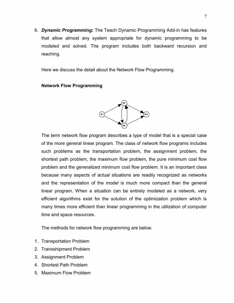
Network Flow Programming

The term network flow program describes a type of model that is a special case

of the more general linear program. The class of network flow programs includes

such problems as the transportation problem, the assignment problem, the

shortest path problem, the maximum flow problem, the pure minimum cost flow

problem and the generalized minimum cost flow problem. It is an important class

because many aspects of actual situations are readily recognized as networks

and the representation of the model is much more compact than the general

linear program. When a situation can be entirely modeled as a network, very

efficient algorithms exist for the solution of the optimization problem which is

many times more efficient than linear programming in the utilization of computer

time and space resources.

The methods for network flow programming are below.

1. Transportation Problem

2. Transshipment Problem

3. Assignment Problem

4. Shortest Path Problem

5. Maximum Flow Problem

8


Transportation problem is one of the subclasses of Linear Programming

Problem(LPP) in which the objective is to transport various quantities of a single

homogeneous commodity that are initially stored at various origins to different

destinations in such a way that the total transportation cost is minimum. To

achieve this objective we must know the amount and location of available

supplies and the quantities demanded. In addition, we must know the costs that

result from transporting one unit of commodity from various origins to various

destinations.

1.2.1 Mathematical Formulation of the Transportation Problem

A Transportation Problem can be stated mathematically as a Linear

Programming Problem as below:

��

��

�

��

Subject to the constraints

� �� , i=1,2,…,m (supply constraints)

� �� !�� , j=1,2,…,n (demand constraints)

xij ≥ 0 for all i and j

Where, ai = quantity of commodity available at origin i

bj= quantity of commodity demanded at destination j

cij= cost of transporting one unit of commodity from ith origin to jth

destination

xij = quantity transported from ith origin to jth destination


In the transportation problems, it was assumed that a source (factory, plant etc.)

acts only as a shipper of the goods and a destination (market etc.) acts only as

receiver of the goods. We shall now consider the broader class of transportation

9

problem, called as transshipment problem, which allow for the shipment of goods

both from one source to another, and from one destination point to another.

Thus, the possibility of transshipment-the goods produced/available at one

source and destined for some destination point may reach there via other

sources and/or destinations and transshipped at these points. This is obviously a

more realistic statement of the distribution problem faced by a business/industrial

house. For example, a multi-plant firm may find it necessary to send some goods

from one plant to another in order to meet the substantial increase in the demand

in the second marker. The second plant here would act both as a source and a

destination and there is no real distinction between source and destination.

A transportation problem can be converted into a transshipment problem by

relaxing the restrictions on the receiving and sending the units on the origins and

destinations respectively. An m-origin, n-destination, transportation problem,

when expressed as a transshipment problem: with m+n origins and an equal

number of destinations. With minor modifications, this problem can be solved

using the transportation method. In a transportation problem, shipment of

commodity takes place among sources and destinations. But instead of direct

shipments to destinations, the commodity can be transported to a particular

destination through one or more intermediate or trans-shipment points. Each of

these points in turn supply to other points. Thus, when the shipments pass from

destination to destination and from source to source, we have a trans-shipment

problem.

In a transportation problem, shipments are allowed only between source-sink

pairs. In many applications, this assumption is too strong. For example, it is often

the case that shipments may be allowed between sources and between sinks.

Moreover, there may also exist points through which units of a product can be

transshipped from a source to a sink. Models with these additional features are

called transshipment problems. Interestingly, it turns out that any given

transshipment problem can be converted easily into an equivalent transportation

10

problem. The availability of such a conversion procedure significantly broadens

the applicability of algorithm for solving transportation problem.

Since Transshipment problem is a particular case of Transportation problem and

hence the mathematical format of the Transshipment problem is similar to date of

Transportation problem.


Imagine, if in a printing press there is one machine and one operator so as to

operate. Immediately a question arrays how would you employ the worker? Your

immediate answer will be, the available operator will operate the machine. Again

suppose there are two machines in the press and two operators are engaged at

different rates to operate them. Which operator should operate which machine for

maximizing profit? Similarly, if there are n machines available and n persons are

engaged at different rates to operate them. Which operator should be assigned

to which machine to ensure maximum efficiency? While answering the above

questions we have to think about the interest of the press, so we have to find

such an assignment by which the press gets maximum profit on minimum

investment. Such problems are known as "assignment problems".

1.4.1 Mathematical Formulation of the Assignment Problem

A assignment problem can be stated mathematically as a Linear Programming

Problem as below:

The objective function is to,

Minimize (Maximize) Z = ∑∑= =

n

i

n

j

ijij xc1 1

Subject to the constraints,

)(,1

)(,1

1

1

trequiremenjobjallforx

tyavailabiliresourceiallforx

n

i

ij

n

j

ij

=

=

∑

∑

=

=

11

Where, xij=0 or 1 and cij represents the cost of assignment from resource i to

activity j.


The Traveling Salesman Problem (TSP) is a problem in combinatorial

optimization studied in operations research and theoretical computer science.

Given a list of cities and their pair wise distances, the task is to find a shortest

possible tour that visits each city exactly once.

The problem was first formulated as a mathematical problem by Menger (1930)

and is one of the most intensively studied problems in optimization. It is used as

a benchmark for many optimization methods. Even though the problem is

computationally difficult, a large number of heuristics and exact methods are

known, so that some instances with tens of thousands of cities can be solved.

1.6 SUPPLY CHAIN MANAGEMENT

There seems to be a universal agreement on what a supply chain is? A supply

chain is to be a network of autonomous or semi-autonomous business entities

which is collectively responsible for procurement, manufacturing and distribution

activities associated with one or more families of related products.

A supply chain is a network of facilities that procure raw materials, transform

them into intermediate goods and then final products. Finally deliver the products

to customers through a distribution system.

A supply chain is a network of facilities and distribution options that performs the

functions of procurement of materials, transformation of these materials into

intermediate and finished products, and the distribution of these finished products

to customers.

12

1.7 Definitions of Some Terminology

The following terms are to be defined with reference to the transportation

problem, assignment problem and transshipment problem.

Feasible Solution ( F. S.)

A set of non-negative allocations xij ≥ 0, which satisfies the row and column

restrictions is known as feasible solution.

Basic (Initial) Feasible Solution ( B. F.S.)

A feasible solution to an m-origin and n-destination problem is said to be basic

feasible solution if the number of positive allocations are (m+n–1). If the number

of allocations in a basic feasible solutions are less than (m+n–1), it is called

degenerate basic feasible solution (DBFS) (otherwise non-degenerate).

Optimal Solution

A feasible solution (not necessarily basic) is said to be optimal if it minimizes the

total cost.

13

CHAPTER 2

REVIEW OF LITERATURE

2.1 Introduction

In this chapter, we discussed the work done by Many scientist/statistician

so far in Transportation Problem, Transshipment Problem, Assignment Problem,

Travelling salesman problem and Supply Chain Management till yet.


Ji and Chu (2002) have discussed Dual-Matrix Approach Method to solve

the Transportation Problem as an alternative to the Stepping Stone Method. The

approach considers the dual of the Transportation Model instead of the primal

and then obtains the optimal solution of the dual using Matrix operations hence it

is called dual matrix approach. In this method, the unit transportation cost is

generally indicated on the North-East Corner in each cell. This problem can also

be expressed as a linear programming model as follows.

Minimize total cost Z= ij

m

i

n

j

ij xc∑∑= =1 1

Subject to i

n

j

ij ax ≤∑=1

for i=1, 2,…, m (2.1)

j

m

i

ij bx ≥∑=1

for j=1,2,…,n (2.2)

�� " # Here, all ai and bj are assumed to be positive and cost cij are non-negative.

14

In usual balanced transportation problem, the condition ∑∑==

=n

j

j

m

i

i ba11

must hold true. If this condition is not met then a dummy origin or destination is

generally introduced to make the problem balanced in order to use Stepping

Stone Method. However the dual matrix approach introduced by Ji and chu

(2002) does not required that a transportation problem to be balanced. This

method can be used both for balanced and unbalanced transportation problem.

Because of this reason (2.1) is represented as ≤ and (2.2) as ≥ instead of = for

both cases. This is one of advantage in Ji and Chu (2002) approach over the

Stepping Stone method. The dual matrix approach is similar to that of Stepping

Stone Method where first find an initial feasible solution and then get next

improved solution by assessing all non basic cells until the optimal solution

found.

Adlakha and Kowalski (1999, 2006) suggested an alternative solution

algorithm for solving certain TP based on the theory of absolute point. Recently

Adalkha and Kowalski (2009) presented various rules governing load distribution

for alternate optimal solution in Transportation Problem. The load assignment for

an alternate optimal solution is left mostly on the decision of the practitioner.

They illustrated the structure of alternate solution in a transportation problem

using the shadow price. They also provided a systematic analysis for allocating

loads to obtain and alternate optimal solution.

For this purpose they consider the reduced the SP matrix after deleting

the rows/columns related to the cells fix due to absolute structure of TP. Here

they are interested to determine the minimum amount of load Xij. To determine

this amount, analyze every rows and columns of the reduced optimal SP matrix

to determine a loaded cell, say, (s, t) where � �� $ %��&' or�� $ �'��&( . After

identifying cell st, the value of Xst is set as following.

Xst = bt - � ��&' or Xst = as - � ��&( .

Many problems like multi-commodity transportation problem,

transportation problem with different kind of vehicles, multi-stage transportation

problem and transportation problem with capacity limit are an extension of the

15

classical transportation problem considering the additional special condition.

Solving such problems many optimization techniques are used like dynamic

programming, linear programming and heuristic approaches etc. Brezina et. al.

(2010) developed a method for solving multi-stage transportation problem with

capacity limit that reflects limits of transported materials quantity. They also

developed algorithm to find optimal solution. Further they discussed efficiency of

presented algorithm depends on selection of algorithm used to obtain the starting

solution (Author used VAM).

2.3 Transshipment problem

Orden (1956) introduced the concept and application of Transshipment

Problem. He extended the concept of original transportation problem so as to

include the possibility that is using the concept of Transshipment Problem. In

other words, He argued that any shipping or receiving point is also permitted to

act as an intermediate point. In fact, the transshipment technique is used to find

the shortest route from one point to another point representing the network

diagram.

Rhody (1963) considered Transshipment model as reduced matrix model.

He discussed the Transshipment of pork from various places and then

Transshipment of finished product. He studied the shipment of interregional

competitive position of the hog-pork industry in the United States for finding the

optimal location and its Transshipment.

King and Logan (1964) developed two alternative models namely (1) Raw

Product – Final Product spatial equilibrium model and (2) Modified

Transshipment Model. In this model, they discussed simultaneously the costs of

shipping raw materials, processing and shipping final product. This problem is

related with the location and size of the California cattle slaughtering plants given

the location and quantity of slaughter animals and the final product demand. In

fact, they studied based on optimal location, number and size of processing

plant.

16

Judge et al. (1965) formulated the Transshipment model into general

linear programming model. They developed model based on interregional

Transshipment. They developed the formulation of Transshipment Problem and

then converted it into linear programming model. So as to find optimal location

and optimal number of live stock. They applied interregional model of

transshipment to the live stock industry.

Garg and Prakash (1985) studied time minimizing Transshipment model.

In their study, it is seen that how the optimal time can be achieved while

transshipping the goods from different origins to different destinations.

However Herer and Tzur (2001) discussed dynamic Transshipment

Problem. In the standard form, the Transshipment problem is basically a linear

minimum cost network through problem. For such types of optimization

problems, a number of effective solutions are available in the literature since

many years.

Recently Khurana and Arora (2011) observed that the Transshipment

problem is basically a linear minimum cost network problem optimization

technique is required with different constraints. Hence they developed

Transshipment problem model with mixed constraints.

In this method, we have discussed a simple and alternate method for

solving Transshipment Problem which gives an optimal solution.


Konig (1931) developed and introduced a method for solving an

Assignment Problem. He gave his name as Hungarian Method (because he was

a Hungarian Mathematician). He developed the method as an efficient method of

finding the optimal solution without having to make a direct comparison of every

solution. His method works on the principal of reducing the given cost matrix to a

matrix of opportunity cost. Opportunity costs show the relative penalties

associated with assigning resource to an activity as opposed to making the best

or least cost assignment. He further said that if we can reduced the cost matrix to

17

the extent of having at least one zero in each row and each column then it will be

possible to make an optimal assignment where opportunity cost are zero. We

have discussed an algorithm of Hungarian Method for obtaining an optimal

solution of an optimal solution of an Assignment Problem is chapter 5.

The Hungarian method is a combinatorial optimization algorithm which

solves the assignment problem in polynomial time and which anticipated later

primal-dual methods. Kuhn (1955) further developed the assignment problem

which has been as "Hungarian method" because the algorithm was largely based

on the earlier works of two Hungarian mathematicians: Dénes Kınig and Jenı

Egerváry.

James Munkres (1957) reviewed the algorithm and observed that it is

(strongly) polynomial. Since then the algorithm has been known also as Kuhn–

Munkres algorithm or Munkres assignment algorithm. The time complexity of the

original algorithm was O (n4), however Edmonds and Karp, and independently

Tomizawa noticed that it can be modified to achieve an O (n3) running time.

Ford and Fulkerson extended the method to general transportation problems. In

2006, it was discovered that Carl Gustav Jacobi had solved the assignment

problem in the 19th century, and published posthumously in 1890 in Latin.

Thompson (1981) discussed a Recursive method for solving assignment

problems which is a polynomially bounded non simplex method for solving

assignment problems. This method begins by finding the optimal solution for a

problem defined from the first row and they finding the optimum for a problem

defined from rows one, two and so on until it solves the problem consisting of all

rows. Hence it is a dimensional expanding rather than an improvement method. It

has been shown that the row duals are non-increasing and the column duals

non-decreasing. However this work was also published online in 2001.

Li and Smith (1995) have studied facility layout and location problems with

stochastic congestion in the traffic circulation system. They developed an

algorithm for Quadratic Assignment Problems. The algorithm for quadratic

assignment problem is in fact a heuristic algorithm which they used for solving

the complex problems for in traffic circulation system. The advantage of their

18

algorithm was that the algorithm can be used for solving large scale Quadratic

Assignment Problems with reasonable computing times and efficient

performance. They claimed that their method is straight forward approach.

Ji et. al. (1997) discussed a new algorithm for the assignment problem

which they also called an alternative to the Hungarian Method. There assignment

algorithm is based on a 2n*2n matrix where operations are performed on the

matrix until an optimal solution is found.


Hamilton (1856) studied the Travelling Salesman Problem by finding Pak

and Circuits on the dodecahedral graph, which satisfied certain conditions like

adjacency condition etc. Hamilton (1856) also introduced Icosian game which

was marketed in 1859. This game was based on dodecahedral graph of the

adjacency condition.

Menger (1930) studied Hamiltonian Path, in which he has discussed

messenger problem. In messenger problem, he has discussed how to solve a

postman problem as well as many travelers problem. Further he carried out to

find shortest path joining all of a finite set of points where pair wise distances are

known. However his work was unnoticed until and unless his book “ the

Travelling Salesman Problem” was published during 1931-32 in journal. So

Monger was the first person who introduced the name “Travelling Salesman

Problem”.


Oliver and Webber (1982) introduced the term Supply Chain

Management. They further developed the Supply Chain Management system to

express the need to integrate the key business processes from end user through

original suppliers. Being those provides products, services and information that

add values for Customers and other stake holders. The basic idea behind Supply

19

Chain Management is that companies and collaboration involved themselves in a

Supply Chain by exchanging information regarding marketing fluctuation and

production capability.

20

CHAPTER 3

NEW ALTERNATE METHODS OF TRANSPORTATION

PROBLEM

3.1 Introduction

The transportation problem and cycle canceling methods are classical in

optimization. The usual attributions are to the 1940's and later. However, Tolsto

(1930) was a pioneer in operations research and hence wrote a book on

transportation planning which was published by the National Commissariat of

Transportation of the Soviet Union, an article called Methods of ending the

minimal total kilometrage in cargo-transportation planning in space, in which he

studied the transportation problem and described a number of solution

approaches, including the, now well-known, idea that an optimum solution does

not have any negative-cost cycle in its residual graph. He might have been the

first to observe that the cycle condition is necessary for optimality. Moreover, he

assumed, but did not explicitly state or prove, the fact that checking the cycle

condition is also sufficient for optimality.

The transportation problem is concerned with finding an optimal

distribution plan for a single commodity. A given supply of the commodity is

available at a number of sources, there is a specified demand for the commodity

at each of a number of destinations, and the transportation cost between each

source-destination pair is known. In the simplest case, the unit transportation

cost is constant. The problem is to find the optimal distribution plan for

transporting the products from sources to destinations that minimizes the total

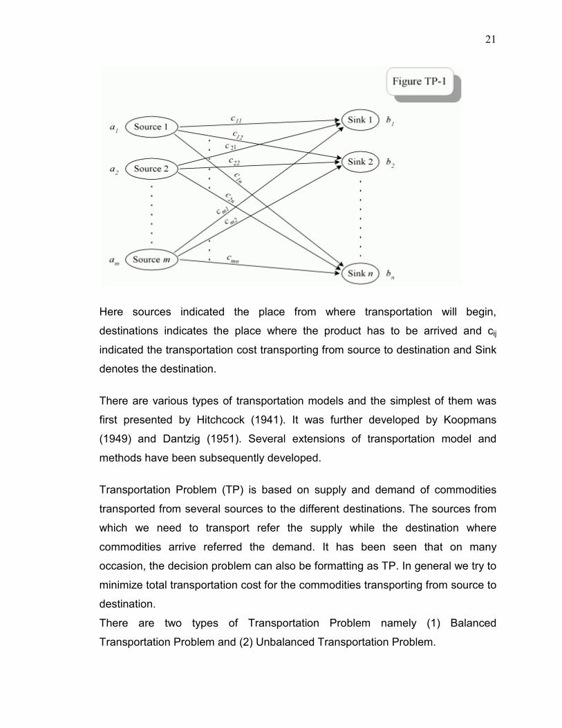
transportation cost. This can be seen in Figure 1.

21

Here sources indicated the place from where transportation will begin,

destinations indicates the place where the product has to be arrived and cij

indicated the transportation cost transporting from source to destination and Sink

denotes the destination.

There are various types of transportation models and the simplest of them was

first presented by Hitchcock (1941). It was further developed by Koopmans

(1949) and Dantzig (1951). Several extensions of transportation model and

methods have been subsequently developed.

Transportation Problem (TP) is based on supply and demand of commodities

transported from several sources to the different destinations. The sources from

which we need to transport refer the supply while the destination where

commodities arrive referred the demand. It has been seen that on many

occasion, the decision problem can also be formatting as TP. In general we try to

minimize total transportation cost for the commodities transporting from source to

destination.

There are two types of Transportation Problem namely (1) Balanced

Transportation Problem and (2) Unbalanced Transportation Problem.

22

Definition of Balanced Transportation Problem: A Transportation Problem is

said to be balanced transportation problem if total number of supply is same as

total number of demand.

Definition of Unbalanced Transportation Problem: A Transportation Problem

is said to be unbalanced transportation problem if total number of supply is not

same as total number of demand.

TP can also be formulated as linear programming problem that can be

solved using either dual simplex or Big M method. Sometimes this can also be

solved using interior approach method. However it is difficult to get the solution

using all this method. There are many methods for solving TP. Vogel’s method

gives approximate solution while MODI and Stepping Stone (SS) method are

considered as a standard technique for obtaining to optimal solution. Since

decade these two methods are being used for solving TP. Goyal (1984)

improving VAM for the Unbalanced Transportation Problem, Ramakrishnan

(1988) discussed some improvement to Goyal’s Modified Vogel’s Approximation

method for Unbalanced Transportation Problem. Moreover Sultan (1988) and

Sultan and Goyal (1988) studied initial basic feasible solution and resolution of

degeneracy in Transportation Problem. Few researchers have tried to give their

alternate method for over coming major obstacles over MODI and SS method.

Adlakha and Kowalski (1999, 2006) suggested an alternative solution algorithm

for solving certain TP based on the theory of absolute point. Ji and Chu (2002)

discussed a new approach so called Dual Matrix Approach to solve the

Transportation Problem which gives also an optimal solution. Recently Adlakha

and Kowalski (2009) suggested a systematic analysis for allocating loads to

obtain an alternate optimal solution. However study on alternate optimal solution

is limited in the literature of TP. In this chapter we have tried an attempt to

provide two alternate algorithms for solving TP. It seems that the methods

discussed by us in this chapter are simple and a state forward. We observed that

for certain TP, our method gives the optimal solution. However for another

23

certain TP, it gives the near to optimal solution. In this chapter we have

discussed only balanced transportation problem for minimization case however

these two methods can also be used for maximization case. Moreover, we may

also use these two methods for unbalanced transportation problem for

minimization and maximization case.


The classical transportation problem can be stated mathematically as follows:

Let ai denotes quantity of product available at origin i, bj denotes quantity of

product required at destination j, Cij denotes the cost of transporting one unit of

product from source/origin i to destination j and xij denotes the quantity

transported from origin i to destination j.

Assumptions: ∑∑==

=n

j

j

m

i

i ba11

This means that the total quantity available at the origins is precisely equal to the

total amount required at the destinations. This type of problem is known as

balanced transportation problem. When they are not equal, the problem is called

unbalanced transportation problem. Unbalanced transportation problems are

then converted into balanced transportation problem using the dummy variables.

3.2.1 Standard form of Transportation Problem as L. P. Problem

Here the transportation problem can be stated as a linear programming problem

as:

Minimise total cost Z= ij

m

i

n

j

ij xc∑∑= =1 1

Subject to i

n

j

ij ax =∑=1

for i=1, 2,…, m

24

j

m

i

ij bx =∑=1

for j=1,2,…,n

and xij ≥0 for all i=1, 2,…, m and j=1,2,…,n

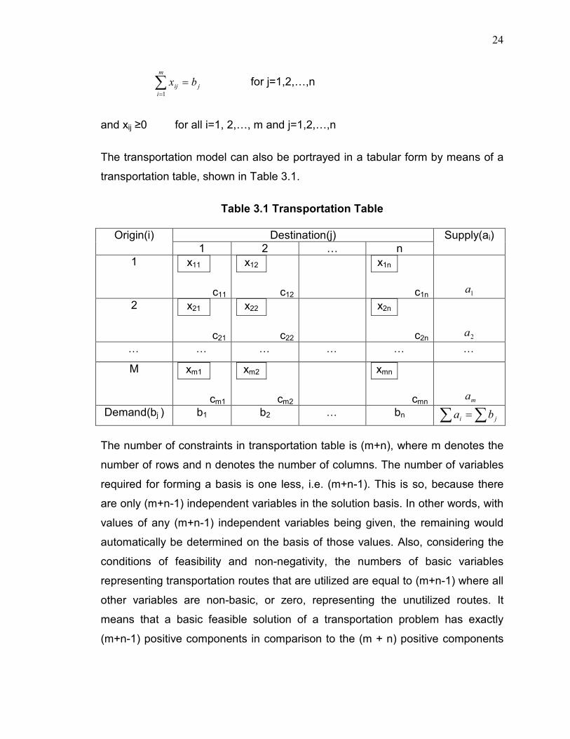
The transportation model can also be portrayed in a tabular form by means of a

transportation table, shown in Table 3.1.

Table 3.1 Transportation Table

Origin(i) Destination(j) Supply(ai) 1 2 … n

1 x11

c11

x12

c12

x1n

c1n

1a

2 x21

c21

x22

c22

x2n

c2n

2a

K K K K K K

M xm1

cm1

xm2

cm2

xmn

cmn

ma

Demand(bj ) b1 b2 K bn ∑∑ = ji ba

The number of constraints in transportation table is (m+n), where m denotes the

number of rows and n denotes the number of columns. The number of variables

required for forming a basis is one less, i.e. (m+n-1). This is so, because there

are only (m+n-1) independent variables in the solution basis. In other words, with

values of any (m+n-1) independent variables being given, the remaining would

automatically be determined on the basis of those values. Also, considering the

conditions of feasibility and non-negativity, the numbers of basic variables

representing transportation routes that are utilized are equal to (m+n-1) where all

other variables are non-basic, or zero, representing the unutilized routes. It

means that a basic feasible solution of a transportation problem has exactly

(m+n-1) positive components in comparison to the (m + n) positive components

25

required for a basic feasible solution in respect of a general linear programming

problem in which there are (m + n) structural constraints to satisfy.

3.3 Solution of the Transportation Problem

A transportation problem can be solved by two methods, using (a) Simplex

Method and (b) Transportation Method. We shall illustrate this with the help of an

example.

Example 3.3.1 A firm owns facilities at six places. It has manufacturing plants at

places A, B and C with daily production of 50, 40 and 60 units respectively. At

point D, E and F it has three warehouses with daily demands of 20, 95 and 35

units respectively. Per unit shipping costs are given in the following table. If the

firm wants to minimize its total transportation cost, how should it route its

products?

Table 3.2

Warehouse

D E F

Plant

A 6 4 1

B 3 8 7

C 4 4 2

(a) Simplex Method

The given problem can be expressed as an LPP as follows:

Let xij represent the number of units shipped from plant i to warehouse j. Let Z

representing the total cost, it can state the problem as follows.


Minimise Z= 6x11+4x12+1x13+3x21+8x22+7x23+4x31+4x32+2x33

26

Subject to constrains:

x11+x12+x13 =50 x11+x21+x31 =20

x21+x22+x23 =40 x12+x22+x32 =95

x31+x32+x33 =60 x13+x23+x33 =35

xij≥0 for i=1,2,3 and j=1,2,3

Using Simplex method, the solution is going to be very lengthy and a

cumbersome process because of the involvement of a large number of decision

and artificial variables. Hence, for an alternate solution, procedure called the

transportation method which is an efficient one that yields results faster and with

less computational effort.

(b) Transportation Method

The transportation method consists of the following three steps.

1. Obtaining an initial solution, that is to say making an initial assignment in

such a way that a basic feasible solution is obtained.

2. Ascertaining whether it is optimal or not, by determining opportunity costs

associated with the empty cells, and if the solution is not optimal.

3. Revising the solution until an optimal solution is obtained.

3.3.1 Methods for Obtaining Basic Feasible Solution for Transportation

Problem

The first step in using the transportation method is to obtain a feasible solution,

namely, the one that satisfies the rim requirements (i.e. the requirements of

demand and supply). The initial feasible solution can be obtained by several

methods. The commonly used are

(I). North – west Corner Method

(II). Least Cost Method (LCM)

27

(III). Vogel’s Approximation Method (VAM)

(I) North-West corner method (NWCM)

The North West corner rule is a method for computing a basic feasible solution of

a transportation problem where the basic variables are selected from the North –

West corner (i.e., top left corner).

Steps

1. Select the north west (upper left-hand) corner cell of the transportation

table and allocate as many units as possible equal to the minimum

between available supply and demand requirements, i.e., min (s1, d1).

2. Adjust the supply and demand numbers in the respective rows and

columns allocation.

3. If the supply for the first row is exhausted then move down to the first

cell in the second row.

4. If the demand for the first cell is satisfied then move horizontally to the

next cell in the second column.

5. If for any cell supply equals demand then the next allocation can be

made in cell either in the next row or column.

6. Continue the procedure until the total available quantity is fully allocated

to the cells as required.

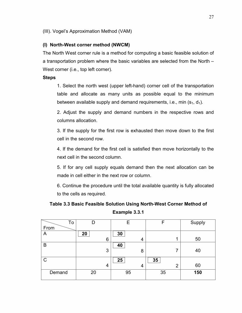
Table 3.3 Basic Feasible Solution Using North-West Corner Method of

Example 3.3.1

To From

D E F Supply

A 20 6

30 4

1

50

B 3

40 8

7

40

C 4

25 4

35 2

60

Demand 20 95 35 150

28

Total Cost: (6*20) + (4*30) + (8*40) + (4*25) + (2*35) = Rs. 730

This routing of the units meets all the rim requirements and entails 5 (=m+n-1 =

3+3-1) shipments as there are 5 occupied cells; It involves a total cost of Rs. 730.

(II) Least Cost Method (LCM)

Matrix minimum method is a method for computing a basic feasible solution of a

transportation problem where the basic variables are chosen according to the

unit cost of transportation.

Steps

1. Identify the box having minimum unit transportation cost (cij).

2. If there are two or more minimum costs, select the row and the column

corresponding to the lower numbered row.

3. If they appear in the same row, select the lower numbered column.

4. Choose the value of the corresponding xij as much as possible subject

to the capacity and requirement constraints.

5. If demand is satisfied, delete that column.

6. If supply is exhausted, delete that row.

7. Repeat steps 1-6 until all restrictions are satisfied.

Table 3.4 Basic Feasible Solution Using Least Cost Method of Example

3.3.1

To From

D E F Supply

A 6

15 4

35 1

50

B 20

3

20 8

7

40

C 4

60 4

2

60

Demand 20 95 35 150

Total Cost: 3*20 + 4*15 + 8*20 +4*60 + 1*35 = Rs. 555

29



(III) Vogel’s Approximation Method (VAM)

The Vogel approximation method is an iterative procedure for computing a basic

feasible solution of the transportation problem.

Steps

1. Identify the boxes having minimum and next to minimum transportation

cost in each row and write the difference (penalty) along the side of the

table against the corresponding row.

2. Identify the boxes having minimum and next to minimum transportation

cost in

each column and write the difference (penalty) against the corresponding

column

3. Identify the maximum penalty. If it is along the side of the table, make

maximum allotment to the box having minimum cost of transportation in

that row. If it is below the table, make maximum allotment to the box

having minimum cost of transportation in that column.

4. If the penalties corresponding to two or more rows or columns are equal,

select the top most row and the extreme left column.

Table 3.5 Basic Feasible Solution Using Vogel’s Method of Example 3.3.1

To From

D E F Supply Iteration I II

A 6

15 4

35 1

50 3 3

B 20

3

20 8

7

40

4

1

C 4

60 4

2

60

2

2

Demand 20 95 35 150 I 1 0 1 II - 0 1

30

Total Cost: 3*20 + 4*15 + 8*20 +4*60 + 1*35 = Rs. 555



3.3.2 Test for Optimality

Once an initial solution is obtained, the next step is to check its optimality.

An optimal solution is one where there is no other set of transportation routes

(allocations) that will further reduce the total transportation cost. Thus, we have

to evaluate each unoccupied cell (represents unused route) in the transportation

table in terms of an opportunity of reducing total transportation cost.

An unoccupied cell with the largest negative opportunity cost is selected to

include in the new set of transportation routes (allocations). This is also known as

an incoming variable. The outgoing variable in the current solution is the

occupied cell (basic variable) in the unique closed path (loop) whose allocation

will become zero first as more units are allocated to the unoccupied cell with

largest negative opportunity cost. Such an exchange reduces total transportation

cost. The process is continued until there is no negative opportunity cost. That is,

the current solution cannot be improved further. This is the optimal solution.

An efficient technique called the modified distribution (MODI) method (also

called u-v method).

Now we discuss MODI method which gives optimal solution and is shown in

3.3.2.1.

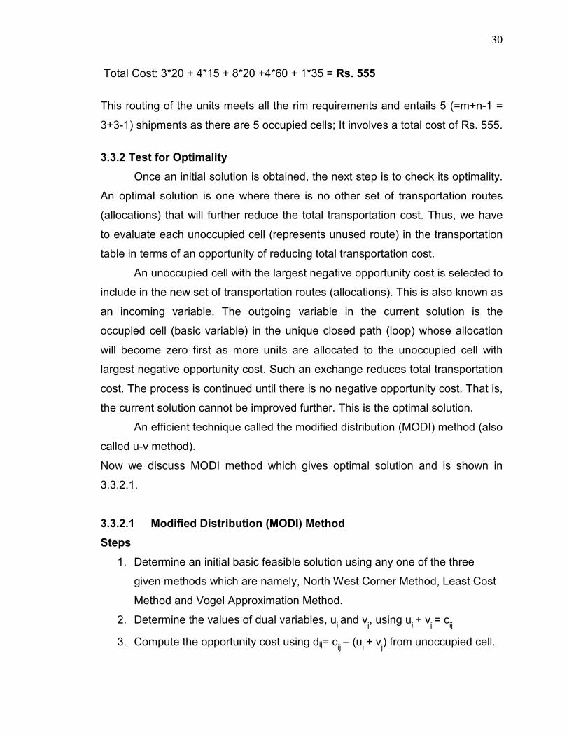
3.3.2.1 Modified Distribution (MODI) Method

Steps

1. Determine an initial basic feasible solution using any one of the three

given methods which are namely, North West Corner Method, Least Cost

Method and Vogel Approximation Method.

2. Determine the values of dual variables, ui and v

j, using u

i + v

j = c

ij

3. Compute the opportunity cost using dij= cij – (ui + v

j) from unoccupied cell.

31

4. Check the sign of each opportunity cost (dij). If the opportunity costs of all

the unoccupied cells are either positive or zero, the given solution is the

optimum solution. On the other hand, if one or more unoccupied cell has

negative opportunity cost, the given solution is not an optimum solution

and further savings in transportation cost are possible.

5. Select the unoccupied cell with the smallest negative opportunity cost as

the cell to be included in the next solution.

6. Draw a closed path or loop for the unoccupied cell selected in the previous

step. Please note that the right angle turn in this path is permitted only at

occupied cells and at the original unoccupied cell.

7. Assign alternate plus and minus signs at the unoccupied cells on the

corner points of the closed path with a plus sign at the cell being

evaluated.

8. Determine the maximum number of units that should be shipped to this

unoccupied cell. The smallest value with a negative position on the closed

path indicates the number of units that can be shipped to the entering cell.

Now, add this quantity to all the cells on the corner points of the closed

path marked with plus signs and subtract it from those cells marked with

minus signs. In this way an unoccupied cell becomes an occupied cell.

9. Repeat the whole procedure until an optimum solution is obtained.

Table 3.6 Optimal Solution Using MODI Method of Example 3.3.1

To From

D E F Supply ui

A 6

15 4

35 1

50 u1=0

B 20 3

20 8

7

40

u2=4

C 4

60 4

2

60

u3=0

Demand 20 95 35 150

vj v1=-1 v2=4 v3=1

32

Total Cost: 3*20 + 4*15 + 8*20 +4*60 + 1*35 = Rs. 555



3.4 NEW ALTERNATE METHOD FOR SOLVING TRANSPORTATION

PROBLEM

So far three general methods for solving transportation methods are available in

literature which is already discussed. These methods give only initial feasible

solution. However here we discuss two new alterative methods which give Initial

feasible solution as well as optimal or nearly optimal solution. Apart from above

three methods, other two methods called MODI method and Stepping Stone

method give the optimal solution. But to get the optimal solution, first of all we

have to find initial solution from either of three methods discussed. However the

methods discussed in this chapter gives initial as well as either optimal solution

or near to optimal solution. In other sense we can say that if we apply any one of

the two methods, it gives either initial feasible solution as well as optimal solution

or near to optimal solution.

3.4.1 Algorithm for Solving Transportation Problem Using New Method

Following are the steps for solving Transportation Problem

Step 1 Select the first row (source) and verify which column (destination) has

minimum unit cost. Write that source under column 1 and corresponding

destination under column 2. Continue this process for each source. However if

any source has more than one same minimum value in different destination then

write all these destination under column 2.

Step 2 Select those rows under column-1 which have unique destination. For

example, under column-1, sources are O1, O2, O3 have minimum unit cost which

represents the destination D1, D1, D3 written under column 2. Here D3 is unique

33

and hence allocate cell (O3, D3) a minimum of demand and supply. For an

example if corresponding to that cell supply is 8, and demand is 6, then allocate

a value 6 for that cell. However, if destinations are not unique then follow step 3.

Next delete that row/column where supply/demand exhausted.

Step 3 If destination under column-2 is not unique then select those sources

where destinations are identical. Next find the difference between minimum and

next minimum unit cost for all those sources where destinations are identical.

Step 4 Check the source which has maximum difference. Select that source and

allocate a minimum of supply and demand to the corresponding destination.

Delete that row/column where supply/demand exhausted.

Remark 1 For two or more than two sources, if the maximum difference happens

to be same then in that case, find the difference between minimum and next to

next minimum unit cost for those sources and select the source having maximum

difference. Allocate a minimum of supply and demand to that cell. Next delete

that row/column where supply/demand exhausted.

Step 5 Repeat steps 3 and 4 for remaining sources and destinations till (m+n-1)

cells are allocated.

Step 6 Total cost is calculated as sum of the product of cost and corresponding

allocated value of supply/ demand. That is,

Total cost = ∑∑= =

n

i

n

j

ijij xc1 1

3.4.2 Numerical Examples

In this section we present a detailed example to illustrated the steps of the

proposed alternate method.

Example 3.4.2.1 Let us consider the Example 3.3.1.

34

A firm owns facilities at six places. It has manufacturing plants at places A, B and

C with daily production of 50, 40 and 60 units respectively. At point D, E and F it

has three warehouses with daily demands of 20, 95 and 35 units respectively.

Per unit shipping costs are given in the following table. If the firm wants to

minimize its total transportation cost, how should it route its products?

Table 3.7

Warehouse D E F

Plant A 6 4 1 B 3 8 7 C 4 4 2

Solution

Step 1 The minimum cost value for the corresponding sources A,B,C are 1, 3

and 2 which represents the destination F, D and F respectively which is shown in

Table 3.8.

Table 3.8

Column 1 Column 2

A F

B D

C F

Step 2 Here the destination D is unique for source B and allocate the cell (B, D)

min (20, 40) =20. This is shown in Table 3.9.

Table 3.9

To From

D E F Supply

A 6

4

1

50

B 20 3

8

7

40

C 4

4

2

60

Demand 20 95 35 150

35

Step 3 Delete column D as for this destination demand is exhausted and adjust

supply as (40-20) =20. Next the minimum cost value for the corresponding

sources A,B,C are 1, 7 and 2 which represents the destination F, F and F

respectively which is shown in Table 3.10.

Table 3.10

Column 1 Column 2

A F

B F

C F

Here the destinations are not unique because sources A, B, C have identical

destination F. so we find the difference between minimum and next minimum unit

cost for the sources A, B and C. The differences are 3, 1 and 2 respectively for

the sources A, B and C.

Step 4: Here the maximum difference is 3 which represents source A. Now

allocate the cell (A, F), min (50, 35) = 35 which is shown Table 3.11.

Table 3.11

To From

E F Supply

A 4

35 1

50

B 8

7

20

C 4

2

60

Demand 95 35 150

Step 5: Delete column F as demand is exhausted. Next adjust supply as (50-35)

=15. Next the minimum unit cost for the corresponding sources A,B and C are 4,

8 and 4 which represents the destination E, E and E respectively which is shown

in Table 3.12.

36

Table 3.12

Column 1 Column 2

A E

B E

C E

Here the source A, B, C have identical destination E, so we must find minimum

difference. However only one column remain and hence minimum difference can

not be obtained. So allocate the remaining supply 15, 20 and 60 to cells (A, E)

(B, E) and (C, E) which is shown in Table 3.13.

Table 3.13

To From

E Supply

A 15 4

15

B 20 8

20

C 60 4

60

Demand 95 150

Step 6: Here (3+3-1) =5 cells are allocated and hence we got our feasible

solution. Next we calculate total cost as some of the product of cost and its

corresponding allocated value of supply/demand which is shown in Table 3.14.

Table 3.14 Basic Feasible Solution using new method

To From

D E F Supply

A 6

15 4

35 1

50

B 20 3

20 8

7

40

C 4

60 4

2

60

Demand 20 95 35 150

37

Total cost: (15*4) + (35*1) + (20*3) + (20*8) + (60*4) = 555

This is a basic feasible solution. The solutions obtained using NCM, LCM, VAM

and MODI/SSM is 730, 555, 555 and 555 respectively. Hence the basic feasible

solution obtained from new method is optimal solution.

Result Our solution is same as that of optimal solution obtained by using LCM,

VAM and MODI/Stepping stone method. Thus our method also gives optimal

solution.

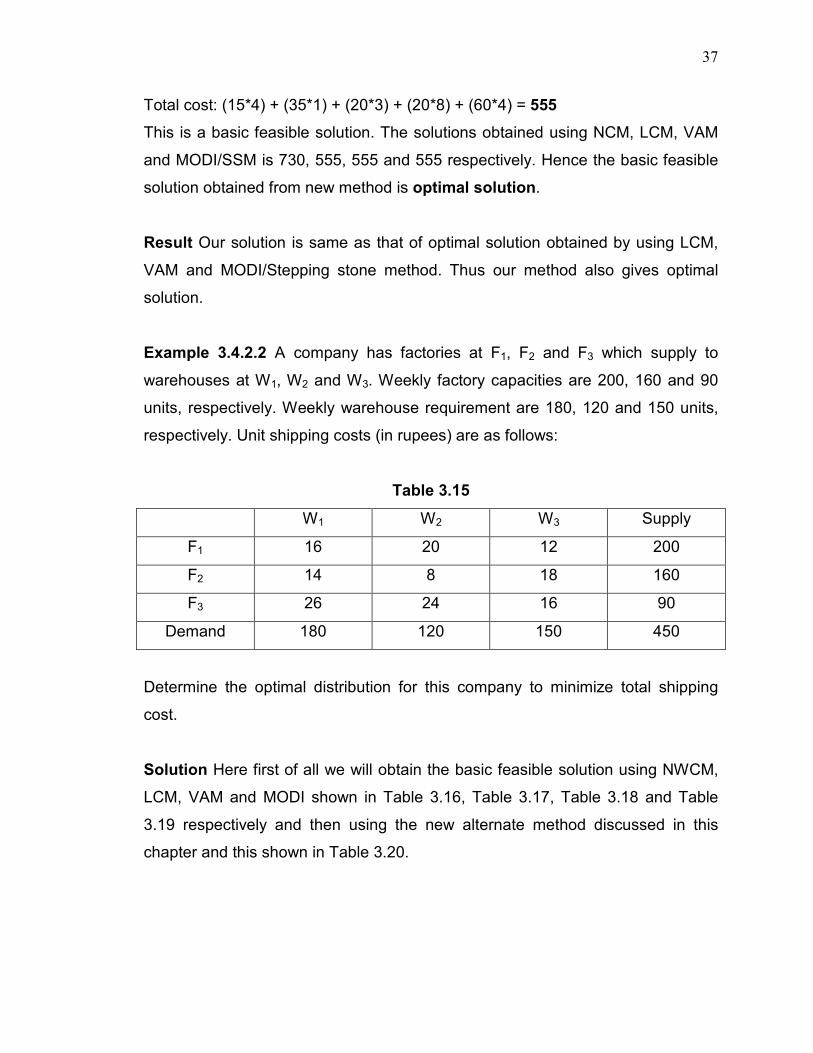
Example 3.4.2.2 A company has factories at F1, F2 and F3 which supply to

warehouses at W1, W2 and W3. Weekly factory capacities are 200, 160 and 90

units, respectively. Weekly warehouse requirement are 180, 120 and 150 units,

respectively. Unit shipping costs (in rupees) are as follows:

Table 3.15

W1 W2 W3 Supply

F1 16 20 12 200

F2 14 8 18 160

F3 26 24 16 90

Demand 180 120 150 450

Determine the optimal distribution for this company to minimize total shipping

cost.

Solution Here first of all we will obtain the basic feasible solution using NWCM,

LCM, VAM and MODI shown in Table 3.16, Table 3.17, Table 3.18 and Table

3.19 respectively and then using the new alternate method discussed in this

chapter and this shown in Table 3.20.

38

3.16 Basic feasible solution using North-West Corner Method

To From

W1 W2 W3 Supply

F1 180 16

20 20

12

200

F2 14

100 8

60 18

160

F3 26

24

90 16

90

Demand 180 120 150 450

Total Cost: (180*16) + (20*20) + (100*8) + (60*18) + (90*16) = 6600

3.17 Basic feasible solution using Least Cost Method

To From

W1 W2 W3 Supply

F1 50 16

20

150 12

200

F2 40 14

120 8

18

160

F3 90 26

24

16

90

Demand 180 120 150 450

Total cost: (50*16) + (150*12) + (40*14) + (120*8) + (90*26) = 6460

3.18 Basic feasible solution using Vogel’s Approximation Method

To From

W1 W2 W3 Supply Iteration

F1 140 16

20

60 12

200

4

4

4

F2 40 14

120 8

18

160

6

4

4

F3 26

24

90 16

90

8

10

-

Demand 180 120 150 450

Iteration

2 12 4

2 - 4

2 - 6

39

Total cost: (140*16) + (60*12) + (40*14) + (120*8) + (90*16) = 5920

3.19 Optimal Solution using MODI Method

To From

W1 W2 W3 Supply ui

F1 140 16

20

60 12

200

u1= 12

F2 40 14

120 8

18

160

u2=10

F3 26

24

90 16

90

u3= 16

Demand 180 120 150 450

vj v1= 4 v2= -2 v3=0

Total Cost= (140*16) + (60*12) + (40*14) + (120*8) + (90*16) = 5920

Now following algorithm 3.4.1, we solve example 3.4.2.2 using new alternate

method and obtained the initial feasible solution which is shown in Table 3.20.

Table 3.20 showing the solution of Example 3.4.2.2 using new alternate

method

To From

W1 W2 W3 Supply

F1 140 16

20

60 12

200

F2 40 14

120 8

18

160

F3 26

24

90 16

90

Demand 180 120 150 450

Total cost= (140*16) + (60*12) + (40*14) + (120*8) + (90*16) = 5920

This is an initial feasible solution. The solutions obtained from NCM, LCM, VAM

and MODI/SSM is 6600, 6460, 5920 and 5920 respectively. Hence the basic

initial feasible solution obtained from new method is optimal solution.

40

Result Our solution is same as that of optimal solution obtained by using VAM

and MODI/Stepping stone method. Thus our method also gives optimal solution.

Now we illustrate some more numerical examples using new alternate method.

Example 3.4.2.3 The following table shows on the availability of supply to each

warehouse and the requirement of each market with transportation cost (in

rupees) from each warehouse to each market. In market demands are 300, 200

and 200 units while the warehouse has supply for 100, 300 and 300 units.

Table 3.21

K1 K2 K3 Supply R1 5 4 3 100 R2 8 4 3 300 R3 9 7 5 300

Demand 300 200 200 700

Determine the total cost for transporting from warehouse to market.

Solution: Now following algorithm 3.4.1, we solve example 3.4.2.3 using new

alternate method and obtained the Basic feasible solution which is shown in

Table 3.22.


method

K1 K2 K3 Supply R1 100

5

4

3

100

R2 100

8

200

4

3

300

R3 100

9

7

200

5

300

Demand 300 200 200 700

41

Total cost= (100*5) + (100*8) + (200*4) + (100*9) + (200*5) =

500+800+800+900+1000= 4000.

This is a basic initial feasible solution. The solutions obtained from NCM, LCM,

VAM and MODI/SSM is 4200, 4100, 3900 and 3900 respectively. Hence the

basic initial feasible solution obtained from new method is near to optimal

solution.

Result Our solution is least than that of NWCM and LCM, while more than VAM

and MODI/Stepping stone method. Thus our method gives near to optimal

solution.

Example 3.4.2.4 Determine an initial feasible solution to the following

transportation problem where Oi and Dj represent ith origin and jth destination,

respectively.

Table 3.23

Destination

D1 D2 D3 D4 Supply

Origin

O1 6 4 1 5 14

O2 8 9 2 7 16

O3 4 3 6 2 5

Demand 6 10 15 4 35

Solution Now following algorithm 3.4.1, we solve example 3.4.2.4 using new


Table 3.24.

42


method

D1 D2 D3 D4 Supply O1 5

6

9 4

1

5

14

O2 1 8

9

15 2

7

16

O3 4

1

3

6

4

2

5

Demand 6 10 15 4 35

Total cost= (6*5) + (9*4) + (1*8) + (15*2) + (1*3) + (4*2) = 30+36+8+30+3+8 =

115.

This is a basic feasible solution. The solutions obtained from NCM, LCM, VAM

and MODI/SSM is 128, 156, 114 and 114 respectively. Hence the basic feasible

solution obtained from new method is near to optimal solution.

Result Our solution is least than that of NWCM and LCM, while more than VAM

and MODI/Stepping stone method. Thus our method gives near to optimal

solution.

Example 3.4.2.5 The following table shows all the necessary information on the

availability of supply to each warehouse, the requirement of each market and unit

transportation cost (in Rs) from each warehouse to each market.

Table 3.25

Market Supply

P Q R S

Warehouse

A 6 3 5 4 22

B 5 9 2 7 15

C 5 7 8 6 8

Demand 7 12 17 9 45

Determine minimum cost value for this transportation problem.

43



Table 3.26.


method

Market Supply P Q R S

Warehouse

A

6

12

3

2

5

8

4

22

B

5

9

15

2

7

15

C

7

5

7

8

1

6

8

Demand 7 12 17 9 45

Total cost= (12*3)+(2*5)+(8*4)+(15*2)+(7*5)+(1*6) = 149

This is a basic feasible solution. The solutions obtained from NCM, LCM, VAM

and MODI/SSM is 176, 150, 149 and 149 respectively. Hence the basic initial

feasible solution obtained from new method is optimal solution.

Result The solution obtained for example 3.4.2.5 using new alternate method is

same as that of optimal solution obtained using VAM and MODI/Stepping stone

method. Thus the method discussed in this chapter also gives same optimal

solution.

3.5 ANOTHER NEW ALTERNATE METHOD (MINIMUM DEMAND-SUPPLY

METHOD) FOR SOLVING TRANSPORTATION PROBLEM

In section 3.4 we discussed a new alternate method for solving a TP based on

unique activity. Next we discussed another new alternate method which is based

44

on minimum demand-supply techniques. For this purpose, we explain algorithm

for solving Transportation Problem in 3.5.1.

3.5.1 Algorithm for solving Transportation Problem using alternate method:

Following are the steps for solving Transportation Problem

Step1 Formulate the problem and set up in the matrix form. The formulation of

TP is similar to that of LPP. So objective function is the total transportation cost

and constraints are the supply and demand available at each source and

destination respectively.

Step 2 Select that row/column where supply/demand is minimum. Find the

minimum cost value in that respective row/column. Allocate minimum of supply

demand to that cell.

Step 3 Adjust the supply/demand accordingly.

Step 4 Delete that row/column where supply/demand is exhausted.

Step 5 Continue steps 1 to step 3 till (m+n-1) cells are allocate.

Step 6 Total cost is calculated as sum of the product of cost and corresponding

assigned value of supply / demand. That is, Total cost = ∑∑= =

n

i

n

j

ijij xc1 1

Remark The new alternate method discussed in this section is optimal for certain

TP while it gives initial feasible solution only for another certain TP.

3.5.2 Numerical Examples

Example 3.5.2.1 A firm owns facilities at six places. It has manufacturing plants

at places A, B and C with daily production of 50, 40 and 60 units respectively. At

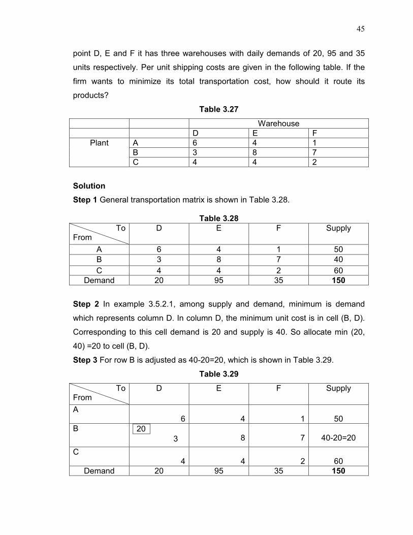
45

point D, E and F it has three warehouses with daily demands of 20, 95 and 35

units respectively. Per unit shipping costs are given in the following table. If the

firm wants to minimize its total transportation cost, how should it route its

products?

Table 3.27

Warehouse D E F

Plant A 6 4 1 B 3 8 7 C 4 4 2

Solution

Step 1 General transportation matrix is shown in Table 3.28.

Table 3.28

To From

D E F Supply

A 6 4 1 50 B 3 8 7 40 C 4 4 2 60

Demand 20 95 35 150

Step 2 In example 3.5.2.1, among supply and demand, minimum is demand

which represents column D. In column D, the minimum unit cost is in cell (B, D).

Corresponding to this cell demand is 20 and supply is 40. So allocate min (20,

40) =20 to cell (B, D).

Step 3 For row B is adjusted as 40-20=20, which is shown in Table 3.29.

Table 3.29

To From

D E F Supply

A 6

4

1

50

B 20 3

8

7

40-20=20

C 4

4

2

60

Demand 20 95 35 150

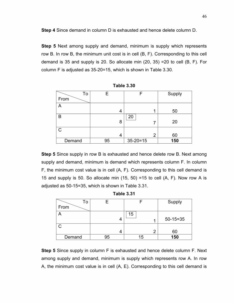
46

Step 4 Since demand in column D is exhausted and hence delete column D.

Step 5 Next among supply and demand, minimum is supply which represents

row B. In row B, the minimum unit cost is in cell (B, F). Corresponding to this cell

demand is 35 and supply is 20. So allocate min (20, 35) =20 to cell (B, F). For

column F is adjusted as 35-20=15, which is shown in Table 3.30.

Table 3.30

To From

E F Supply

A 4

1

50

B 8

20 7

20

C 4

2

60

Demand 95 35-20=15 150

Step 5 Since supply in row B is exhausted and hence delete row B. Next among

supply and demand, minimum is demand which represents column F. In column

F, the minimum cost value is in cell (A, F). Corresponding to this cell demand is

15 and supply is 50. So allocate min (15, 50) =15 to cell (A, F). Now row A is

adjusted as 50-15=35, which is shown in Table 3.31.

Table 3.31

To From

E F Supply

A 4

15

1

50-15=35

C 4

2

60

Demand 95 15 150

Step 5 Since supply in column F is exhausted and hence delete column F. Next

among supply and demand, minimum is supply which represents row A. In row

A, the minimum cost value is in cell (A, E). Corresponding to this cell demand is

47

95 and supply is 35. So allocate min (95, 35) =35 to cell (A, E). Now column E is

adjusted as 95-35=60, which is shown in Table 3.32.

Table 3.32

To From

E Supply

A 35 4

35

C 4

60

Demand 95-35=60 150

Step 5 Here only one cell C is remains so allocate min (60, 60) =60 to cell (C, E).

The final allocated supply and demand is shown in Table 3.33.

Table 3.33 Basic feasible solution using another new method

To From

D E F Supply

A 6

35 4

15

1

50

B 20

3

8

20 7

40 20

C 4

60

4

2

60

Demand 20 95 35 15 150

In Table 3.33, (3+3-1) =5 cells are allocate and hence we got our feasible

solution.

Step 5 Total cost: (35*4) + (15*1) + (20*3) + (20*7) + (60*4) = 595

The solution obtained in our method is less than NWCM but grater than LCM,

VAM and MODI. Hence it is better than NWC method and gives near to optimal

solution.

Example 3.5.2.2 A company has factories at F1, F2 and F3 which supply to

warehouses at W1, W2 and W3. Weekly factory capacities are 200, 160 and 90

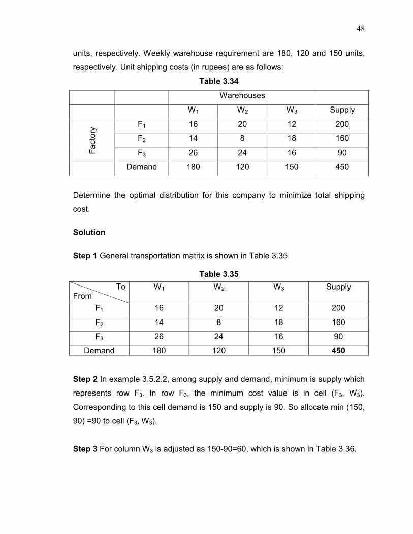
48

units, respectively. Weekly warehouse requirement are 180, 120 and 150 units,

respectively. Unit shipping costs (in rupees) are as follows:

Table 3.34

Warehouses

W1 W2 W3 Supply

Fac

tory F1 16 20 12 200

F2 14 8 18 160

F3 26 24 16 90

Demand 180 120 150 450

Determine the optimal distribution for this company to minimize total shipping

cost.

Solution

Step 1 General transportation matrix is shown in Table 3.35

Table 3.35

Step 2 In example 3.5.2.2, among supply and demand, minimum is supply which

represents row F3. In row F3, the minimum cost value is in cell (F3, W3).


90) =90 to cell (F3, W3).

Step 3 For column W3 is adjusted as 150-90=60, which is shown in Table 3.36.

To From

W1 W2 W3 Supply

F1 16 20 12 200

F2 14 8 18 160

F3 26 24 16 90

Demand 180 120 150 450

49

Table 3.36

To From

W1 W2 W3 Supply

F1 16 20 12 200

F2 14 8 18 160

F3 26

24

90 16

90

Demand 180 120 150-90=60 450

Step 4 Since supply in row F3 is exhausted and hence delete row F3.

Step 5 Next among supply and demand, minimum is demand which represents

column W3. In column W3, the minimum cost value is in cell (F1, W3).


200) =60 to cell (F1, W3). For row F1 is adjusted as 200-60=140, which is shown

in Table 3.37.

Table 3.37

Step 5 Since demand in column W3 is exhausted and hence delete column W3.

Next among supply and demand, minimum is demand which represents column

W2. In column W2, the minimum cost value is in cell (F2, W2). Corresponding to

this cell demand is 120 and supply is 160. So allocate min (120, 160) =120 to cell

(F2, W2). Now row F2 is adjusted as 160-120=40, which is shown in Table 3.38.

To From

W1 W2 W3 Supply

F1 16

20

60 12

200-60=140

F2 14 8 18 160

Demand 180 120 60 450

50

Table 3.38

To From

W1 W2 Supply

F1 16

20

140

F2 14

120 8

160-120=40

Demand 180 120 450

Step 5 Since demand in column W2 is exhausted and hence delete column W2.

Next among supply and demand, minimum is supply which represents row F2. In

row F2, the minimum cost value is in cell (F2, W1). Corresponding to this cell

demand is 180 and supply is 40. So allocate min (180, 40) =40 to cell (F2, W1).

Now column W1 is adjusted as 180-40=140, which is shown in Table 3.39.

Table 3.39

To From

W1 Supply

F1 16

140

F2 40 14

40

Demand 180-40=140 450

Step 5 Here only one cell (F1, W1) is remains so allocate min (140, 140) =140.

The final allocated supply and demand is shown in Table 3.40.


To From

W1 W2 W3 Supply

F1

140 16

20

60 12

200

F2 40 14

120 8

18

160

F3 26

24

90 16

90

Demand 180 120 150 450

In Table 3.40, (3+3-1) =5 cells are allocate and hence we achieved feasible

solution.

51

Total cost= (140*16) + (60*12) +(40*14)+(120*8)+(90*16) = 5920


VAM and MODI/SSM is 6600, 6460, 5920 and 5920 respectively. Hence the

basic initial feasible solution obtained from new method is optimal solution.

Result: Our solution is same as that of optimal solution obtained by using VAM

and MODI/Stepping stone method. Thus our method also gives optimal solution.

Remark We have solved example 3.4.2.1(3.5.2.1) using both the new alternate

methods discussed in 3.4 and 3.5. However we got the same optimal solution

from both the methods. This proves that both methods give optimal solution for

certain TP.

Example 3.5.2.3: The following table shows on the availability of supply to each

warehouse and the requirement of each market with transportation cost (in

rupees) from each warehouse to each market. In market demands are 300, 200

and 200 units while the warehouse has supply for 100, 300 and 300 units.

Table 3.38

K1 K2 K3 R1

5 4

3

R2 8

4

3

R3 9

7

5

Determine the total cost for transporting from warehouse to market.

Solution Now following algorithm 3.5.1, we solve example 3.5.2.3 (using another

new alternate method) and obtained the Basic feasible solution which is shown in

Table 3.39.

52


K1 K2 K3 Supply R1

5

4 100

3 100

R2 8

200 4

100 3

300

R3 300 9

7

5

300

Demand 300 200 200 700 Total cost: (100*3) + (200*4) + (100*3) + (300*9) = 300+800+300+2700 = 4100 This value is same as obtained from LCM while better than NWCM but more than

VAM/MODI method. This solution is happened to be near to optimal solution

as we get directly from new alternate method.

Example 3.5.2.4 Determine an initial feasible solution to the following

transportation problem where Oi and Dj represent ith origin and jth destination,

respectively.

Table 3.40

D1 D2 D3 D4 Supply

O1 6 4 1 5 14

O2 8 9 2 7 16

O3 4 3 6 2 5

Demand 6 10 15 4 35



Table 3.41.

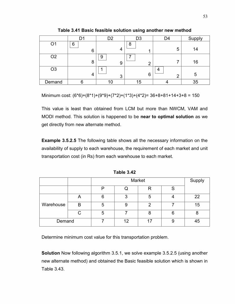
53


D1 D2 D3 D4 Supply O1 6

6

4

8

1

5

14

O2 8

9 9

7

2

7

16

O3 4

1

3

6

4

2

5

Demand 6 10 15 4 35

Minimum cost: (6*6)+(8*1)+(9*9)+(7*2)+(1*3)+(4*2)= 36+8+81+14+3+8 = 150

This value is least than obtained from LCM but more than NWCM, VAM and

MODI method. This solution is happened to be near to optimal solution as we

get directly from new alternate method.

Example 3.5.2.5 The following table shows all the necessary information on the

availability of supply to each warehouse, the requirement of each market and unit

transportation cost (in Rs) from each warehouse to each market.

Table 3.42

Market Supply

P Q R S

Warehouse

A 6 3 5 4 22

B 5 9 2 7 15

C 5 7 8 6 8

Demand 7 12 17 9 45

Determine minimum cost value for this transportation problem.



Table 3.43.

54


Market Supply P Q R S

Warehouse

A 6

12

3

2

5

8

4

22

B 5

9

15

2

7

15

C 7

5

7

8

1

6

8

Demand 7 12 17 9 45

Total cost= (12*3)+(2*5)+(8*4)+(15*2)+(7*5)+(1*6) = 149


VAM and MODI/SSM is 176, 150, 149 and 149 respectively. Hence the basic

initial feasible solution obtained from new method is optimal solution.

Table 3.44 shows comparison of total cost of transportation problem

obtained from various methods

Examples Method 1 Method 2 NWCM LCM VAM MODI

3.6.2.1 555 595 730 555 555 555

3.6.2.2 5920 5920 6600 6460 5920 5920

3.6.2.3 4000 4100 4200 4100 3900 3900

3.6.2.4 115 150 128 156 114 114

3.6.2.5 149 149 176 150 149 149

Remark From Table 3.44, it is clear that method 1 gives optimal solution for

almost all examples while method 2 gives optimal solution for certain examples

of TP.

55

3.6 Conclusion

This chapter deals two alternate algorithms for TP as very few alternate

algorithms for obtaining an optimal solution are available in the textbook and in

other literature. These methods are so simple and easy that makes

understandable to a wider spectrum of readers. The methods discussed in this

chapter give a near optimal solution for certain TP while it gives optimal solution

for other certain TP.

56

CHAPTER 4

A NEW ALTERNATE METHOD OF TRANS-SHIPMENT

PROBLEM

4.1 Introduction

In a transportation problem shipment of commodity takes place among

sources and destinations. But instead of direct shipments to destinations, the

commodity can be transported to a particular destination through one or more

intermediate or trans-shipment points. Each of these points in turn supply to

other points. Thus, when the shipments pass from destination to destination and

from source to source, we have a trans-shipment problem. Since transshipment

problem is a particular case of transportation problem hence to solve

transshipment problem, we first convert transshipment problem into equivalent

transportation problem and then solve it to obtain optimal solution using MODI

method of transportation problem. In a transportation problem, shipments are

allowed only between source-sink pairs. In many applications, this assumption is

too strong. For example, it is often the case that shipments may be allowed

between sources and between sinks. Moreover, some points may exist through

which units of a product can be transshipped from a source to a sink. Models

with these additional features are called transshipment problems. Interestingly, it

turns out that any given transshipment problem can be converted easily into an

equivalent transportation problem. The availability of such a conversion

procedure significantly broadens the applicability of our algorithm for solving

transportation problems.

A transportation problem allows only shipments that go directly from

supply points to demand points. In many situations, shipments are allowed

between supply points or between demand points. Sometimes there may also be

57

points (called transshipment points) through which goods can be transshipped on

their journey from a supply point to a demand point. Fortunately, the optimal

solution to a transshipment problem can be found by solving a transportation

problem.

Some Definition:

Supply point: It can send goods to another point but cannot receive goods from

any other point.

Demand point: It can receive goods from other points but cannot send goods to

any other point.

Transshipment point: It can both receive goods from other points send goods

to other points.

Orden (1956) introduced the concept of Transshipment Problem. He

extended the concept of original transportation problem so as to include the

possibility of transshipment. In other words, we can say that any shipping or

receiving point is also permitted to act as an intermediate point. In fact, the

transshipment technique is used to find the shortest route from one point to

another point representing the network diagram. Rhody (1963) considered

Transshipment model as reduced matrix model. King and Logan (1964) argued

that the problem of determining simultaneously the flows of primary products

through processor to the market as final product has been formulated

alternatively as a transshipment model. However Judge et al. (1965) formulated

the Transshipment model into general linear programming model. Garg and

Prakash (1985) studied time minimizing Transshipment model. However Herer

and Tzur (2001) discussed dynamic Transshipment Problem. In the standard

form, the Transshipment problem is basically a linear minimum cost network. For

such types of optimization problems, a number of effective solutions are available

in the literature since many years. Recently Khurana and Arora (2011) discussed

transshipment problem with mixed constraints. In this chapter, we have

58

discussed a simple and alternate method for solving Transshipment Problem

which gives either an optimal solution or near to optimal solution.


If we let the sources and destinations in a transshipment problem as T, then xij

would represent the amount of goods shipped from the ith terminal (Ti) to the jth

terminal (Tj) and cij would represent the unit cost of such shipment. Naturally, xij

would equal to zero because no units would be shipped from a terminal to itself.

Now, assume that at m terminals ( T1, T2, … , Tm), the total out shipment exceeds

the total in shipment by amounts equal to a1, a2, … , am respectively and at the

remaining n terminals (Tm+1, Tm+2, … , Tm+n), the total in shipment exceeds the

total out shipment by amounts bm+1, bm+2, … , bm+n respectively. If the total in

shipment at terminals T1, T2, … , Tm be t1, t2, … , tm respectively and the total out

shipment at the terminals Tm+1, Tm+2, … , Tm+n be tm+1, tm+2, … , tm+n respectively,

we can write the transshipment problem as:

)*+*,*-.�/ � � � 0��!1�

��

!1�

��

Subject to

�� 2 ��3 242 ��5�6� 2 ��5�1� 242 ��5!1� 7 8� � ��* � 95:5 ; 5,��9� �� 2 �3� 242 ��6�5� 2 ��1�5� 242 �!1�5� � 8��* � 95:5 ; 5,��:�

�� 2 �3� 242 ��6�5� 2 ��1�5� 242 �!1�5� 7 8�� < � , 2 95, 2 :5 ; 5, 2 +��=�

�� 2 ��3 242 ��5�6� 2 ��5�1� 242 ��5!1�� 8��< � , 2 95, 2 :5; 5, 2 +��>�

��!

��

!1�

��!1�� ?�

As can be easily observed, these constraints are similar to the constraints of a

transportation problem with m+n sources and m+n destinations, with the

differences that here there are no xii and xjj terms, and that bj=0 for j=1,2,…,m

59

and ai = 0 for i=m+1,m+2,…,m+n. The terms ti and tj in these constraints may be

seen as the algebraic equivalents of xii and xjj. Now, we can view this problem as

an enlarged problem and solve it by using the transportation method.

The transshipment problem can be depicted form as shown in Table 4.1.

Table 4.1 Transshipment Problem

Terminal

Ti↓ Tj→

1 2 … m m+1 … m+n Supply

ai

1 -t1 x12 … x1m x1,m+1 … x1,m+n a1

2 x21 -t1 … x2m x2,m+1 … x2,m+n a2

` ` `

m xm1 xm2 -tm xm,m+1 xm,m+1 am

m+1 xm+1,1 xm+1,2 xm+1,m -tm+1 xm+1,m+n 0

` ` `

m+n xm+n,1 xm+n,2 xm+n,m xm+n,m+1 -tm+n 0

Demand

bj

0 0 … 0 bm+1 … bm+n ∑ai=∑bj

The first m rows represent the m constraints given in (1) while the remaining n

rows show the constraints given in (4). The constraints in (2) and (3) are

represented by the first m columns and the remaining n columns respectively. All

the t values are placed on the diagonal from left top to right bottom. Each of them

bears negative sign which must be considered carefully when a t is involved in

the readjustment (during the solution process).

4.3 Solution of the Transshipment Problem

The following are steps for solving a Transshipment problem so far available in

the literature.

Step1 If necessary, add a dummy demand point (with a supply of 0 and a

demand equal to the problem’s excess supply) to balance the problem.

Shipments to the dummy and from a point to itself will be zero. Let s= total

available supply.

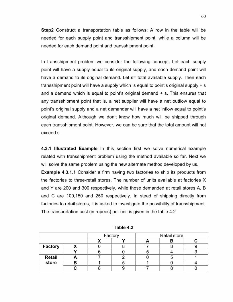
60

Step2 Construct a transportation table as follows: A row in the table will be

needed for each supply point and transshipment point, while a column will be

needed for each demand point and transshipment point.

In transshipment problem we consider the following concept. Let each supply

point will have a supply equal to its original supply, and each demand point will

have a demand to its original demand. Let s= total available supply. Then each

transshipment point will have a supply which is equal to point’s original supply + s

and a demand which is equal to point’s original demand + s. This ensures that

any transshipment point that is, a net supplier will have a net outflow equal to

point’s original supply and a net demander will have a net inflow equal to point’s

original demand. Although we don’t know how much will be shipped through

each transshipment point. However, we can be sure that the total amount will not

exceed s.

4.3.1 Illustrated Example In this section first we solve numerical example

related with transshipment problem using the method available so far. Next we

will solve the same problem using the new alternate method developed by us.

Example 4.3.1.1 Consider a firm having two factories to ship its products from

the factories to three-retail stores. The number of units available at factories X

and Y are 200 and 300 respectively, while those demanded at retail stores A, B

and C are 100,150 and 250 respectively. In stead of shipping directly from

factories to retail stores, it is asked to investigate the possibility of transshipment.

The transportation cost (in rupees) per unit is given in the table 4.2

Table 4.2

Factory Retail store X Y A B C

Factory X 0 8 7 8 9 Y 6 0 5 4 3

Retail store

A 7 2 0 5 1 B 1 5 1 0 4 C 8 9 7 8 0

61

Find the optimal shipping schedule.

Solution We solve this problem using VAM to find the initial solution and then

use this initial solution to obtain optimal solution using MODI method in the

following way.

Table 4.3 showing Initial solution using VAM

X Y A B C Supply X 0

0

8 100

7 100

8

9

200 Y

6 0

0

5 50

4 250

3 300

A 7

2

0 0

5

1

0

B 1

5

1

0 0

4

0

C 8

9

7

8

0 0

0

Demand 0 0 100 150 250 500

Table 4.4 showing optimal solution using MODI

X Y A B C Supply ui X 0

0

8

100

7

100

8

9

200

u1=4

Y 6

0

0

5

50

4

250

3

300 u2=0

A 7

2

0

0

5

1

0 u3=-3

B 1

5

1

0

0

4

0 u4=-4

C 8

9

7

8

0

0

0 u5=-3

Demand 0 0 100 150 250 500 vj v1=-4 v2=0 v3=3 v4=4 v5=3

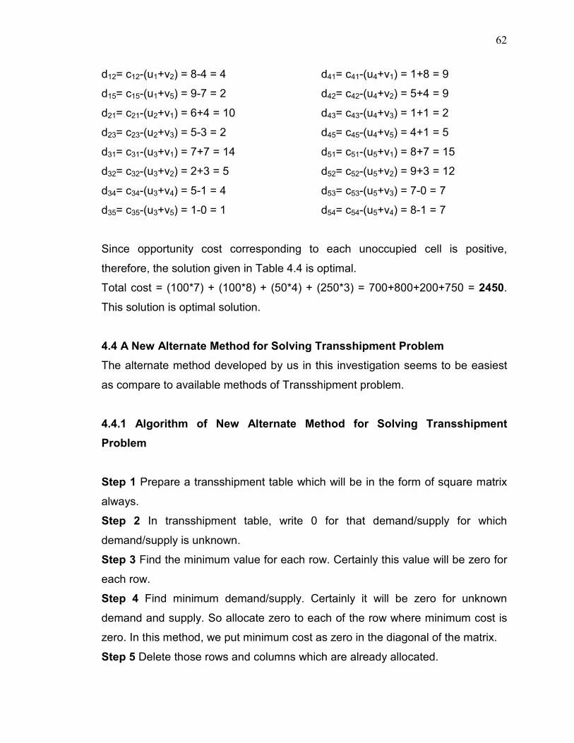
62

d12= c12-(u1+v2) = 8-4 = 4

d15= c15-(u1+v5) = 9-7 = 2

d21= c21-(u2+v1) = 6+4 = 10

d23= c23-(u2+v3) = 5-3 = 2

d31= c31-(u3+v1) = 7+7 = 14

d32= c32-(u3+v2) = 2+3 = 5

d34= c34-(u3+v4) = 5-1 = 4

d35= c35-(u3+v5) = 1-0 = 1

d41= c41-(u4+v1) = 1+8 = 9

d42= c42-(u4+v2) = 5+4 = 9

d43= c43-(u4+v3) = 1+1 = 2

d45= c45-(u4+v5) = 4+1 = 5

d51= c51-(u5+v1) = 8+7 = 15

d52= c52-(u5+v2) = 9+3 = 12

d53= c53-(u5+v3) = 7-0 = 7

d54= c54-(u5+v4) = 8-1 = 7

Since opportunity cost corresponding to each unoccupied cell is positive,

therefore, the solution given in Table 4.4 is optimal.

Total cost = (100*7) + (100*8) + (50*4) + (250*3) = 700+800+200+750 = 2450.

This solution is optimal solution.

4.4 A New Alternate Method for Solving Transshipment Problem

The alternate method developed by us in this investigation seems to be easiest

as compare to available methods of Transshipment problem.

4.4.1 Algorithm of New Alternate Method for Solving Transshipment

Problem

Step 1 Prepare a transshipment table which will be in the form of square matrix

always.

Step 2 In transshipment table, write 0 for that demand/supply for which

demand/supply is unknown.

Step 3 Find the minimum value for each row. Certainly this value will be zero for

each row.

Step 4 Find minimum demand/supply. Certainly it will be zero for unknown

demand and supply. So allocate zero to each of the row where minimum cost is

zero. In this method, we put minimum cost as zero in the diagonal of the matrix.

Step 5 Delete those rows and columns which are already allocated.

63

Step 6 Find minimum unit cost for remaining rows. If minimum unit cost is distinct

then allocate min (supply, demand) to that cell. For example, let for row x

minimum unit cost is 3 in column B and for row y minimum unit cost is 2 in

column A. So allocate min (supply, demand) to cell (x, B) and cell (y, A). If it is

not distinct then go to step 7.

Step 7 Delete those rows and columns where supply and demand exhausted.

Next adjust supply/demand for undeleted row/column. If they are not distinct then

find difference between minimum and next minimum unit cost for those rows

where they are identical. Find the maximum difference and allocate those cells

where demand/supply is minimum. For example, column B contains the minimum

unit cost for row x and y. For row x, difference between minimum and next

minimum unit cost is 2 while for row y, difference between minimum and next

minimum unit cost is 1, so 2 is maximum and hence allocate a min( supply,

demand) to cell (x, B).

Step 8 Continue steps 6 and 7 until (m+n-1) cells are allocated. This gives initial

feasible solution.

Step 9 Find total cost as sum of the product of allocated demand/supply and cost

value for the respective cells. That is,

@A8�B�0AC8 � � � 0��!1�

��

!1�

��D�

This total cost gives optimal or near to optimal solution.

4.4.2 Numeric Examples

Example 4.4.2.1 Consider the example 4.3.1.1.

Solution We solve this Transshipment problem using new alternate method in

following steps.

Step 1 Table 4.5 shows the Transshipment matrix

Step 2 In table 4.5 write zero for unknown demand/supply for respective column

of the row.

Step 3 The minimum cost value in each row is zero.

64

Step 4 We find that zero is minimum unit cost in each row and hence allocate

zero in the diagonal cell of the Transshipment matrix .Which are shown in Table

4.5.

Table 4.5 Transshipment Matrix


0 8

7

8

9

200

Y 6

0 0

5

4

3

300

A 7

2

0 0

5

1

0

B 1

5

1

0 0

4

0

C 8

9

7

8

0 0

0

Demand 0 0 100 150 250 500 Step 5 Delete columns X, Y and rows A, B, C. The remaining is shown in Table 4.6.

Table 4.6

A B C Supply X 7 8 9 200 Y 5 4 3 300

Demand 100 150 250 500

Step 6 In row X, the minimum unit cost is 7 which represents column A. Similarly

in row Y, the minimum unit cost is 3 which represents column C. So allocate min

(100, 200) = 100 to cell (X, A) and a min (250, 300) = 250 to cell (Y, C). Next

adjust the supply for rows X and Y which is shown in Table 4.7.

Table 4.7

A B C Supply X

100 7

8

9

200-100=100

Y

5

4

250

3

300-250=50

Demand 100-100=0 150 250-250=0 500 Delete column A and C. Next, the minimum unit cost in rows X and Y are 8 and 4

respectively which represent column B. So allocate min (100, 150) =100 to cell

65

(X, B). Remaining demand for column B is 150-100=50 which is to be allocated

to cell (Y, B). Finally in Table 4.8 we showed that (5+5-1) =9 cells are occupied

and hence we get initial feasible solution.

Table 4.8 Basic feasible solution using new method


0

8 100

7 100

8

9

200

Y 6

0 0

5

50 4

250 3

300

A 7

2

0 0

5

1

0

B 1

5

1

0 0

4

0

C 8

9

7

8

0 0

0

Demand 0 0 100 150 250 500 Total cost = (100*7) + (100*8) + (50*4) + (250*3) = 700+800+200+750 = 2450.

Result This gives an optimal solution. This is similar to that of MODI method.

Example 4.4.2.2 A firm owns facilities at six places. It has manufacturing plants

at places A, b, and C with daily production of 50, 40 and 60 units respectively. At

point D, E and F, it has three warehouses with daily demands of 20, 95 and 35

units respectively. The firm instead of shipping from plant to warehouse decides

to investigate the possibility of trans-shipment. The unit transportation cost (in

Rs) is given in the table 4.9.

Table 4.9

Plant Warehouse Supply

A B C D E F

Plant A 0 3 2 6 4 1 50 B 3 0 4 3 8 7 40 C 2 4 0 4 4 2 60

Warehouse D 6 3 4 0 2 5 0 E 4 8 4 2 0 1 0 F 1 7 2 5 1 0 0

Demand 0 0 0 50 40 60 150

66



Table 4.10.


Total cost: (50*1) + (40*3) + (10*4) + (40*4) + (10*2) = 50+120+40+160+20 =

390.


Example 4.4.2.3 A firm having two sources, S1 and S2 wishes to ship its product

to two destinations, D1 and D2. The number of units available at S1 and S2 are

10 and 30 and the product demanded at D1 and D2 are 25 and 15 units

respectively. The firm instead of shipping from sources to destinations decides to

investigate the possibility of trans-shipment. The unit transportation cost (in Rs) is

given in the table 4.11.

A B C D E F Supply

A 0 0

3

2

6

4

50

1

50

B 3

0 0

4

40 3

8

7

40

C 2

4

0 0

10 4

40 4

10 2

60

D 6

3

4

0 0

2

5

0

E 4

8

4

2

0 0

1

0

F 1

7

2

5

1

0

0

0

Demand 0 0 0 50 40 60 150

67

Table 4.11

Source Destination Supply S1 S2 D1 D2

Source S1 0

3

4

5

10

S2 3

0

3

5

30

Destination D1 4

3

0

2

0

D2 5

5

2

0

0

Demand 0 0 25 15 40

Determine the shipping schedule.



Table 4.10.


Source Destination Supply S1 S2 D1 D2

Source S1 0

0

3

4

10

5

10

S2 3

0

0

25

3

5

5

30

Destination D1 4

3

0

0

2

0

D2 5

5

2

0

0

0

Demand 0 0 25 15 40

Total minimum cost = (10*5) + (25*3) + (5*5) = 50+75+25=150.


68

4.5 Conclusion

In this chapter we have developed a simple algorithm for solving a

Transshipment Problem. The proposed algorithm is easy to understand and

apply. The optimal solution obtained in this investigation is same as that of MODI

method.

69

CHAPTER 5

A NEW ALTERNATE METHOD OF ASSIGNMENT PROBLEM

5.1 Introduction

An assignment problem is a particular case of transportation problem

where the objective is to assign a number of resources to an equal number of

activities so as to minimize total cost or maximize total profit of allocation.

The problem of assignment arises because available resources such as men,

machines, etc. have varying degrees of efficiency for performing different

activities. Therefore, cost, profit or time of performing the different activities is

different. Thus, the problem is how the assignments should be made so as to

optimize the given objective. The assignment problem is one of the

fundamental combinatorial optimization problems in the branch

of optimization or operations research in Mathematics. It consists of finding a

maximum weight matching in a weighted bipartite graph.

In general, the assignment problem is of following type:

There are a number of agents and a number of tasks. Any agent can be

assigned to perform any task, incurring some cost that may vary depending on

the agent-task assignment. In such problem, it is required to perform all tasks by

assigning exactly one agent to each task in such a way that the total cost of the

assignment is minimized. If the numbers of agents and tasks are equal and the

total cost of the assignment for all tasks is equal to the sum of the costs for each

agent (or the sum of the costs for each task, which is the same thing in this

case), then the problem is called the linear assignment problem. Commonly,

when speaking of the assignment problem without any additional qualification,

then the linear assignment problem is meant.

70

Suppose that a taxi firm has three taxis (the agents) available, and three

customers (the tasks) wishing to be picked up as soon as possible. The firm

prides itself on speedy pickups, so for each taxi the "cost" of picking up a

particular customer will depend on the time taken for the taxi to reach the pickup

point. The solution to the assignment problem will be whichever combination of

taxis and customers results in the least total cost. However, the assignment

problem can be made rather more flexible than it first appears. In the above

example, suppose that there are four taxis available, but still only three

customers. Then a fourth dummy task can be invented, perhaps called "sitting

still doing nothing", with a cost of 0 for the taxi assigned to it. The assignment

problem can then be solved in the usual way and still give the best solution to the

problem. Similar tricks can be played in order to allow more tasks than agents,

tasks to which multiple agents must be assigned (for instance, a group of more

customers than will fit in one taxi), or maximizing profit rather than minimizing

cost.

So far in the literature, there are mainly four methods so called Enumeration

Method, Simplex Method, Transportation Method and Hungarian Method for

solving Assignment Problem. Out of which Hungarian method is one of the best

available for solving an assignment problem.

Hungarian mathematician Konig (1931) developed the Hungarian method

of assignment which provides us an efficient method of finding the optimal

solution without having to make a direct comparison of every solution. It works on

the principle of reducing the given cost matrix to a matrix of opportunity costs.

Opportunity costs show the relative penalties associated with assigning resource

to an activity as opposed to making the best or least cost assignment. If we can

reduce the cost matrix to the extent of having at least one zero in each row and

column, it will be possible to make optimal assignments (opportunity costs are all

zero). The Hungarian method is a combinatorial optimization algorithm which

solves the assignment problem in polynomial time and which anticipated later

primal-dual methods. Kuhn (1955) further developed the assignment problem

which has been as "Hungarian method" because the algorithm was largely based

71

on the earlier works of two Hungarian mathematicians: Dénes Kınig and Jenı

Egerváry. Ford and Fulkerson (1956) extended the method to general

transportation problems. Munkres (1957) reviewed the algorithm and observed

that it is strongly polynomial. Since then the algorithm has been known also as

Kuhn–Munkres algorithm or Munkres assignment algorithm. The time complexity

of the original algorithm was O (n4), however Edmonds and Karp (1972) studied

the theoretical improvements in algorithmic efficiency for network flow problems

while Tomizawa (1990b) studied polynomial diagonal-parameter symmetry model

for a square contingency table however both of them independently noticed that

it can be modified to achieve an O(n3) running time. In 2006, it was discovered

that Carl Gustav Jacobi (1890) had solved the assignment problem in the 19th

century but it was not published during his tenure however it was published

posthumously in 1890 in Latin. Jacobi (1890) developed the concept of

assignment algorithm.

Thompson (1981) discussed a recursive method for solving assignment

problem which is a polynomially bounded non simplex method for solving

assignment problem. Li and Smith (1995) discuss an algorithm for Quadratic

assignment problem. Ji et. al. (1997) discussed a new algorithm for the

assignment problem which they also called an alternative to the Hungarian

Method. There assignment algorithm is based on a 2n*2n matrix where

operations are performed on the matrix until an optimal solution is found.

In this chapter, we have developed an alternative method for solving an

assignment problem to achieve the optimal solution. It has been found that the

optimal solution obtained in this method is same as that of Hungarian method.


Given n resources (or facilities) and n activities (or jobs), and effectiveness (in

terms of cost, profit, time, etc.) of each resource (facility) for each activity (job),

72

the problem lies in assigning each resource to one and only one activity (job) so

that the given measure of effectiveness is optimized. The data matrix for this

problem is shown in Table 5.1.

Table 5.1 Data Matrix

Resources

(workers)

Activities(jobs) Supply

J1 J2 K Jn

W1 c11 c12 K c1n 1

W2 c21 c22 K c2n 1

M M M M M

Wn cn1 cn2 K cnn 1

Demand 1 1 K 1 n

From Table 5.1, it may be noted that the data matrix is the same as the

transportation cost matrix except that supply (or availability) of each of the

resources and the demand at each of the destinations is taken to be one. It is

due to this fact that assignments are made on a one-to-one basis.

Let xij denote the assignment of facility i to job j such that

xij =

otherwise

jjobtoassignedisifacilityif

0

1

Then, the mathematical model of the assignment problem can be stated as:


Minimise Z = ∑∑= =

n

i

n

j

ijij xc1 1

Subject to the constraints

)(,1

)(,1

1

1

trequiremenactivityjallforx

tyavailabiliresourceiallforx

n

i

ij

n

j

ij

=

=

∑

∑

=

=

73

Where, xij=0 or 1 and cij represents the cost of assignment of resource i to activity

j.

From the above discussion, it is clear that the assignment problem is a variation

of the transportation problem with two characteristics: (i) the cost matrix is a

square matrix, and (ii) the optimal solution for the problem would always be such

that there would be only one assignment in a given row or column of the cost

matrix.

5.3 Solution of the Assignment Problem

So far, in the literature it is available that an assignment problem can be solved

by the following four methods.

I. Enumeration method

II. Simplex method

III. Transportation method

IV. Hungarian method

Here, we discuss each of four, one by one.

I. Enumeration method

In this method, a list of all possible assignments among the given resources (like

men, machines, etc.) and activities (like jobs, sales areas, etc.) is prepared. Then

an assignment involving the minimum cost (or maximum profit), time or distance

is selected. If two or more assignments have the same minimum cost (or

maximum profit), time or distance, the problem has multiple optimal solutions.

In general, if an assignment problem involves n workers/jobs, then there

are in total n! Possible assignments. As an example, for an n=3 workers/jobs

problem, we have to evaluate a total of 3! or 6 assignments. However, when n is

large, the method is unsuitable for manual calculations. Hence, this method is

suitable only for small n.

74

II. Simplex Method

Since each assignment problem can be formulated as a 0 or 1 which becomes

integer linear programming problem. Such a problem can be solved by the

simplex method also. As can be seen in the general mathematical formulation of

the assignment problem, there are n×n decision variables and n+n or 2n

equalities. In particular, for a problem involving 5 workers/jobs, there will be 25

decision variables and 10 equalities. It is, again, difficult to solve manually.

III. Transportation Method

Since an assignment problem is a special case of the transportation problem, it

can also be solved by transportation methods. However, every basic feasible

solution of a general assignment problem having a square payoff matrix of order

n should have more m+n-1= n+n-1= 2n-1 assignments. But due to the special

structure of this problem, any solution cannot have more than n assignments.

Thus, the assignment problem is inherently degenerate. In order to remove

degeneracy, (n-1) number of dummy allocations will be required in order to

proceed with the transportation method. Thus, the problem of degeneracy at

each solution makes the transportation method computationally inefficient for

solving an assignment problem.

IV. Hungarian Method

Assignment problems can be formulated with techniques of linear programming

and transportation problems. As it has a special structure, it is solved by the

special method called Hungarian method. This method was developed by D.

Konig, a Hungarian mathematician and is therefore known as the Hungarian

method of assignment problem. In order to use this method, one needs to know

only the cost of making all the possible assignments. Each assignment problem

has a matrix (table) associated with it. Normally, the objects (or people) one

wishes to assign are expressed in rows, whereas the columns represent the

tasks (or things) assigned to them. The number in the table would then be the

costs associated with each particular assignment. It may be noted that the

75

assignment problem is a variation of transportation problem with two

characteristics. (i) The cost matrix is a square matrix, and (ii) The optimum

solution for the problem would be such that there would be only one assignment

in a row or column of the cost matrix. Hungarian method is based on the principle

that if a constant is added to the elements of cost matrix, the optimum solution of

the assignment problem is the same as the original problem. Original cost matrix

is reduced to another cost matrix by adding a constant value to the elements of

rows and columns of cost matrix where the total completion time or total cost of

an assignment is zero. This assignment is also referred as the optimum solution

since the optimum solution remains unchanged after the reduction.

Hungarian Method (minimization case) can be summarized in the following steps:

Step 1 Develop the cost table from the given problem

If the number of rows is not equal to the number of columns and vice versa, a

dummy row or dummy column must be added. The assignment costs for dummy

cells are always zero.

Step 2 Find the opportunity cost table

(a) Locate the smallest element in each row of the given cost table and then

subtract that from each element of that row, and

(b) In the reduced matrix obtained from 2(a), locate the smallest element in

each column and then subtract that from each element of that column.

Each row and column now have at least one zero value.

Step 3 Make assignments in the opportunity cost matrix

The procedure of making assignments is as follows:

(a) Examine rows successively until a row with exactly one unmarked zero is

obtained. Make an assignment to this single zero by making a square �

around it.

(b) For each zero value that become assigned, eliminate (strike off) all other

zeros in the same row and/or column.

76

(c) Repeat Steps 3(a) and 3(b) for each column also with exactly single zero

value cells that have not been assigned.

(d) If a row and/or column have two or more unmarked zeros and one cannot

be chosen by inspection, then choose the assigned zero cell arbitrarily.

(e) Continue this process until all zeros in rows/columns are either

enclosed(assigned) or struck off(× )

Step 4 Optimality criterion

If the number of assigned cells is equal to the number of rows/columns, then it is

an optimal solution. The total cost associated with this solution is obtained by

adding original cost figures in the occupied cells.

If a zero cell was chosen arbitrarily in Step 3, there exists an alternative

optimal solution. But if no optimal solution is found, then go to Step 5.

Step 5 Revise the opportunity cost table

Draw a set of horizontal and vertical lines to cover all the zeros in the revised

cost table obtained from Step 3, by using the following procedure:

(a) For each row in which no assignment was made, mark a tick(√)

(b) Examine the marked rows. If any zero cells occur in those rows, mark to

the respective columns that contain those zeros.

(c) Examine marked columns. If any assigned zero occurs in those columns,

tick the respective rows that contain those assigned zeros.

(d) Repeat this process until no more rows or columns can be marked.

(e) Draw a straight line through each marked column and each unmarked

row.

If the number of lines drawn (or total assignments) is equal to the number of rows

(or columns), the current solution is the optimal solution, otherwise go to Step 6.

Step 6 Develop the new revised opportunity cost table

(a) From among the cells not covered by any line, choose the smallest

element. Call this value k.

(b) Subtract k from every element in the cell not covered by a line.

(c) Add k to every element in the cell covered by the two lines, i.e.

intersection of two lines.

77

(d) Elements in cells covered by one line remain unchanged.

Step 7 Repeat Steps 3 to 6 until an optimal solution is obtained.

5.3.1 Solution of Assignment Problem using Hungarian Method

Example 5.3.1.1 A department has five employees with five jobs to be

performed. The time (in hours) each men will take to perform each job is given in

the effectiveness matrix.

Table 5.2

Employees I II III IV V

Jobs

A 10 5 13 15 16 B 3 9 18 13 6 C 10 7 2 2 2 D 7 11 9 7 12 E 7 9 10 4 12

How should the jobs be allocated, one per employee, so as to minimize the total

man-hours? (Refer Sharma, 2007)

Solution Here I solve this example using only Hungarian Method because other

three methods are not mostly used for solving an assignment problem. And then

I show that how our method is better than Hungarian Method.

Applying step 2 of the algorithm, we get the reduced opportunity time matrix as

shown in Table 5.3.

Table 5.3

I II III IV V A 5 0 8 10 11 B 0 6 15 10 3 C 8 5 0 0 0 D 0 4 2 0 5 E 3 5 6 0 8

Steps 3 and 4

(a) We examine all the rows starting from A one-by-one until a row containing

only single zero element is located. Here rows A, B and E have only one zero

78

element in the cells (A, II), (B,I) and (E,IV). Assignment is made in these cells. All

zeros in the assigned columns are now crossed off as shown in Table 5.4.

(b) We now examine each column starting from column 1. There is one zero in

column III, cell (C, III). Assignment is made in this cell. Thus cell (C, V) is crossed

off. All zeros in the table now are either assigned or crossed off as shown in

Table 5.4.

Table 5.4

I II III IV V A 5 0 8 10 11 B 0 6 15 10 3 C 8 5 0 0 × 0 × D 0 × 4 2 0 × 5 E 3 5 6 0 8

The solution is not optimal because only four assignments are made.

Step 5

Cover the zeros with minimum number of lines (=4) as explained below:

(a) Mark (√) row D since it has no assignment.

(b) Mark (√) columns I and IV since row D has zero element in these columns.

(c) Mark (√) rows B and E since columns I and IV have an assignment in rows B

and E, respectively.

(d) Since no other rows or columns can be marked, draw straight lines through

the unmarked rows A and C and the marked columns I and IV, as shown in Table

5.5.

Table 5.5

I II III IV V A 5 0 8 10 11 B 0 6 15 10 3 √ C 8 5 0 0 × 0

×

D 0 × 4 2 0 × 5 √ E 3 5 6 0 8 √ √ √ Step 6

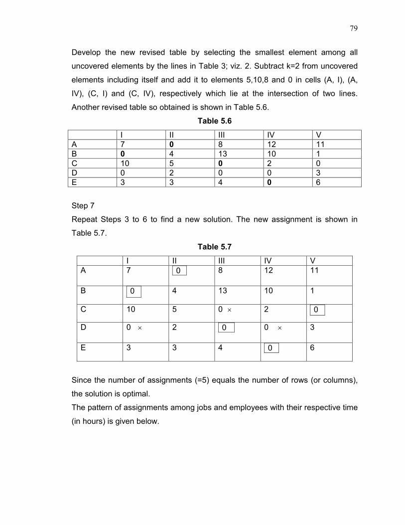
79

Develop the new revised table by selecting the smallest element among all

uncovered elements by the lines in Table 3; viz. 2. Subtract k=2 from uncovered

elements including itself and add it to elements 5,10,8 and 0 in cells (A, I), (A,

IV), (C, I) and (C, IV), respectively which lie at the intersection of two lines.

Another revised table so obtained is shown in Table 5.6.

Table 5.6

I II III IV V A 7 0 8 12 11 B 0 4 13 10 1 C 10 5 0 2 0 D 0 2 0 0 3 E 3 3 4 0 6

Step 7

Repeat Steps 3 to 6 to find a new solution. The new assignment is shown in

Table 5.7.

Table 5.7

I II III IV V A 7 0

8 12 11

B 0

4 13 10 1

C 10 5 0 × 2 0

D 0 × 2 0

0 × 3

E 3 3 4 0

6

Since the number of assignments (=5) equals the number of rows (or columns),

the solution is optimal.

The pattern of assignments among jobs and employees with their respective time

(in hours) is given below.

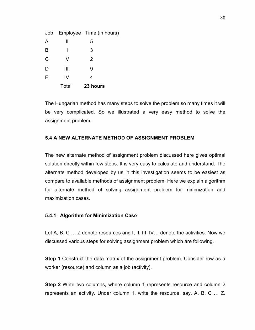
80

Job Employee Time (in hours)

A II 5

B I 3

C V 2

D III 9

E IV 4

Total 23 hours

The Hungarian method has many steps to solve the problem so many times it will

be very complicated. So we illustrated a very easy method to solve the

assignment problem.

5.4 A NEW ALTERNATE METHOD OF ASSIGNMENT PROBLEM

The new alternate method of assignment problem discussed here gives optimal

solution directly within few steps. It is very easy to calculate and understand. The

alternate method developed by us in this investigation seems to be easiest as

compare to available methods of assignment problem. Here we explain algorithm

for alternate method of solving assignment problem for minimization and

maximization cases.

5.4.1 Algorithm for Minimization Case

Let A, B, C … Z denote resources and I, II, III, IV… denote the activities. Now we

discussed various steps for solving assignment problem which are following.

Step 1 Construct the data matrix of the assignment problem. Consider row as a

worker (resource) and column as a job (activity).

Step 2 Write two columns, where column 1 represents resource and column 2

represents an activity. Under column 1, write the resource, say, A, B, C … Z.

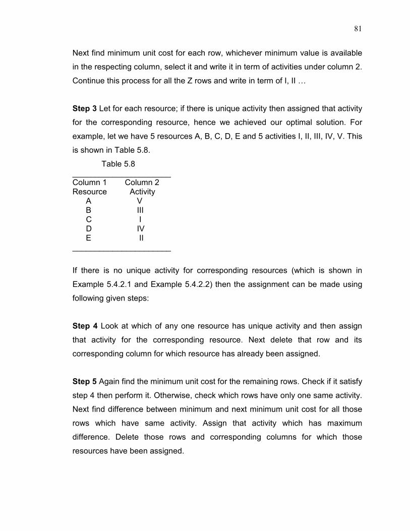
81

Next find minimum unit cost for each row, whichever minimum value is available

in the respecting column, select it and write it in term of activities under column 2.

Continue this process for all the Z rows and write in term of I, II …

Step 3 Let for each resource; if there is unique activity then assigned that activity

for the corresponding resource, hence we achieved our optimal solution. For

example, let we have 5 resources A, B, C, D, E and 5 activities I, II, III, IV, V. This

is shown in Table 5.8.

Table 5.8 ______________________ Column 1 Column 2 Resource Activity A V B III C I D IV E II ______________________

If there is no unique activity for corresponding resources (which is shown in

Example 5.4.2.1 and Example 5.4.2.2) then the assignment can be made using

following given steps:

Step 4 Look at which of any one resource has unique activity and then assign

that activity for the corresponding resource. Next delete that row and its

corresponding column for which resource has already been assigned.

Step 5 Again find the minimum unit cost for the remaining rows. Check if it satisfy

step 4 then perform it. Otherwise, check which rows have only one same activity.

Next find difference between minimum and next minimum unit cost for all those

rows which have same activity. Assign that activity which has maximum

difference. Delete those rows and corresponding columns for which those

resources have been assigned.

82

Remarks 1 However if there is tie in difference for two and more than two activity

then further take the difference between minimum and next to next minimum unit

cost. Next check which activity has maximum difference, assign that activity.

Step 6 Repeat steps 4 to 5 till all jobs are assigned uniquely to the corresponding

activity.

Step 7 Once all the jobs are assigned then calculate the total cost by using the

expression, Total cost = ∑∑= =

n

i

n

j

ijij xc1 1

5.4.2 Numerical Examples In this chapter, we illustrate some numerical

examples to solve the assignment problem using New Alternate Method.

Example 5.4.2.1 A computer centre has five expert programmers. The centre

needs five application programs to be developed. The head of the computer

centre, after studying carefully the programs to be developed. Estimate the

computer time in minutes required by the experts for the application programs.

The observations are shown in Table 5.9.

Table 5.9 Data matrix

Programmers Programs I II III IV V

A 100 90 60 80 120 B 70 90 110 85 105 C 130 110 120 125 140 D 100 120 90 105 85 E 120 140 135 100 115

Assign the programmers to the programs in such a way that the total computer

time is minimum.

Solution Consider Table 5.9, Select row A, where the minimum value is 60

representing program III. Similarly, the minimum value for row-B to row-E are 70,

83

110, 85 and 100 representing programs I, II, V and IV respectively. This is shown

in Table 5.10.

Table 5.10 Table 5.10a

Programmers Programs

A III

B I

C II

D V

E IV

From Table 5.10, we can easily see that different programs are meant for

different programmers. That is, we can assign programs uniquely to the

programmers, which is shown in Table 5.10a and hence we achieved our optimal

solution, which is shown in Table 5.11.

Table 5.11

Programs Programmers Time

I B 70

II C 110

III A 60

IV E 100

V D 85

Total 425

Result This answer is happened to be same as that of Hungarian method.

Hence we can say that the minimum time is still 425 in both the methods. So our

method also gives Optimal Solution. However our method seems to be very

simple, easy and takes very few steps in solving the method.

Programmers Programs

I II III IV V

A 100 90 60

80 120

B 70

90 110 85 105

C 130 110

120 125 140

D 100 120 90 105 85

E 120 140 135 100

115

84

Now we consider another example where (i) different resources do not have

unique activity and (ii) resource has more than one minimum cost. This is

discussed in Example 5.4.2.2.

Example 5.4.2.2 The department has five employees with five jobs to be

performed. The time (in hours) each men will take to perform each job is given in

the effectiveness matrix.


Activities(jobs)

Resources (Employees)

I II III IV V A 10 5 13 15 16 B 3 9 18 13 6 C 10 7 2 2 2 D 7 11 9 7 12 E 7 9 10 4 12

Solution Consider the data matrix 5.12. Now, we select row A and select that

column (activity) for which row A has minimum unit cost. In this example, for row

A, column II (activity) has the minimum unit cast. So we write resource A under

column I and activity II under column II. In the similar way, we select all the rows

(resources) and find the minimum unit cost for the respective columns, which are

shown in Table 5.13.


Resource Activity

A II

B I

C III, IV, V

D I, IV

E IV

Here, Activity II is unique as it doesn’t occur again and hence assigned resource

A to activity II and is shown in Table 5.13a. Next, delete Row A and Column II.

I II III IV V A 10

5

13 15 16

B 3 9 18 13 6 C 10 7 2 2 2 D 7 11 9 7 12 E 7 9 10 4 12

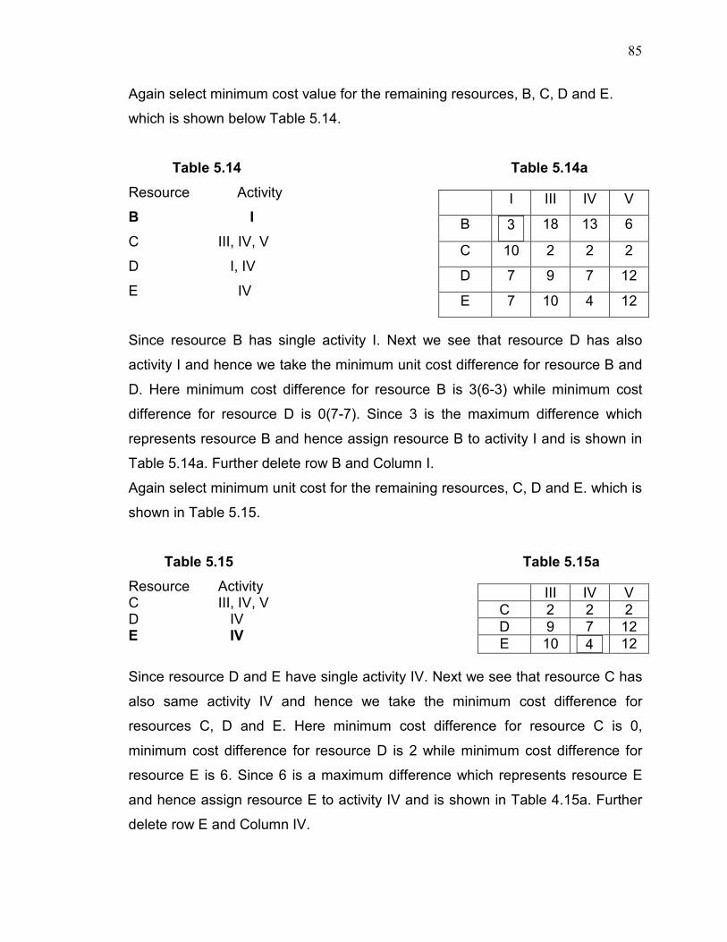
85

Again select minimum cost value for the remaining resources, B, C, D and E.

which is shown below Table 5.14.


Resource Activity

B I

C III, IV, V

D I, IV

E IV

Since resource B has single activity I. Next we see that resource D has also

activity I and hence we take the minimum unit cost difference for resource B and

D. Here minimum cost difference for resource B is 3(6-3) while minimum cost

difference for resource D is 0(7-7). Since 3 is the maximum difference which

represents resource B and hence assign resource B to activity I and is shown in

Table 5.14a. Further delete row B and Column I.

Again select minimum unit cost for the remaining resources, C, D and E. which is



Resource Activity C III, IV, V D IV E IV

Since resource D and E have single activity IV. Next we see that resource C has

also same activity IV and hence we take the minimum cost difference for

resources C, D and E. Here minimum cost difference for resource C is 0,

minimum cost difference for resource D is 2 while minimum cost difference for

resource E is 6. Since 6 is a maximum difference which represents resource E

and hence assign resource E to activity IV and is shown in Table 4.15a. Further

delete row E and Column IV.

I III IV V

B 3

18 13 6

C 10 2 2 2

D 7 9 7 12

E 7 10 4 12

III IV V C 2 2 2 D 9 7 12 E 10 4

12

86

Again select minimum cost value for the remaining resources, C and D. which is



Resource Activity

C III, V

D III

Since resource D has single activity III. Next we see that resource C has also

same activity III and hence we take the minimum cost difference for resources C

and D. Here minimum cost difference for C is 0, while minimum cost difference

for D is 3. Since 3 is the maximum difference which represents resource D and

hence assign resource D to activity III. Finally only row C and column V remains

and hence assign resource C to activity V and is shown in Table 4.16a.

Finally, different employees have assigned jobs uniquely, which is shown in

Table 5.17.

Table 5.17

Employees Jobs Time (in hour) A II 5 B I 3 C V 2 D III 9 E IV 4 Total 23


Hence we can say that the minimum value is still 23 in both the methods. So our


simple, easy and takes very few steps in solving the problem.

Next we consider another example where different resources do not have unique

activity but each resource has only one minimum unit cost. This is discussing in

Example 5.4.2.3.

III V

C 2 2

D 9

12

87

Example 5.4.2.3 A factory has six machines and employed six workers to work

on the given six machines. Based on the workers experience and their personal

efficiency, the workers have assigned to work on six machines. Following is the

times (minutes) taken by workers in completion of that work in the respective

machines. The times are as follow.


Machine I II III IV V VI

Workers

A 9 8 7 5 3 10 B 6 4 2 8 7 9 C 8 10 9 6 4 12 D 9 6 5 4 1 11 E 3 5 6 7 11 8 F 2 4 3 5 8 9

Obtain optimal assignment of the workers.

Solution Consider the data matrix 5.18. Now, we select row A and select that

column (activity) for which row A has minimum value. In this example, for row A,

column V (activity) has the minimum value. So we write resource A under column

I and activity V under column II. In the similar way, we select all the rows

(resources) and find the minimum value for the respective columns. This is


Table 5.19 Table 5.19a Column 1 Column 2 A V B III C V D V E I F I

Here, Activity III is unique as it doesn’t occur again and hence assigned resource

B to activity III and is shown in Table 5.19a. Next, delete Row B and Column III.

I II III IV V VI A 9 8 7 5 3 10 B 6 4 2

8 7 9 C 8 10 9 6 4 12 D 9 6 5 4 1 11

E 3 5 6 7 11 8

F 2 4 3 5 8 9

88

Again select minimum cost value for the remaining resources, A, C, D, E and F.

which is shown below Table 5.20.

Table 5.20 Table 5.20a Column 1 Column 2 A V C V D V E I F I

Since resource A has single activity V. Next we see that resource C and D have

also activity V and hence take the minimum cost difference for resource A, C and

D. Here minimum cost difference for resource A is 2, for resource C is 2, while

minimum cost difference for resource D is 3. Since 3 is the maximum difference

which represents resource D and hence assign resource D to activity V and is

shown in Table 5.20a. Again resource E has single activity I. Next we see that

resource F has also same activity I and hence we take the minimum cost

difference for resource E and F. Here minimum cost difference for resource E is

2 while minimum cost difference for resource F is also 2. So we will find next

minimum difference for resource E and F which comes out as 2 and 1 for E and

F respectively. Since 2 is the maximum difference which represents resource E

and hence assign resource E to activity I and is shown in Table 3a. Further

delete (i) row D and Column V and (ii) row E and Column I.

Again select minimum unit cost for the remaining resources, A, C and F. which is

shown below Table 5.21.

Table 5.21 Table 5.21a Column 1 Column 2 A IV C IV F II

Since resource F has unique single activity II and hence assigned resource F to

activity II shown in Table 5.21a. Further delete row F and Column II. Again select

I II IV V VI A 9 8 5 3 10 C 8 10 6 4 12 D 9 6 4 1

11 E 3

5 7 11 8

F 2 4 5 8 9

II IV VI A 8 5 10 C 10 6 12 F 4

2 9

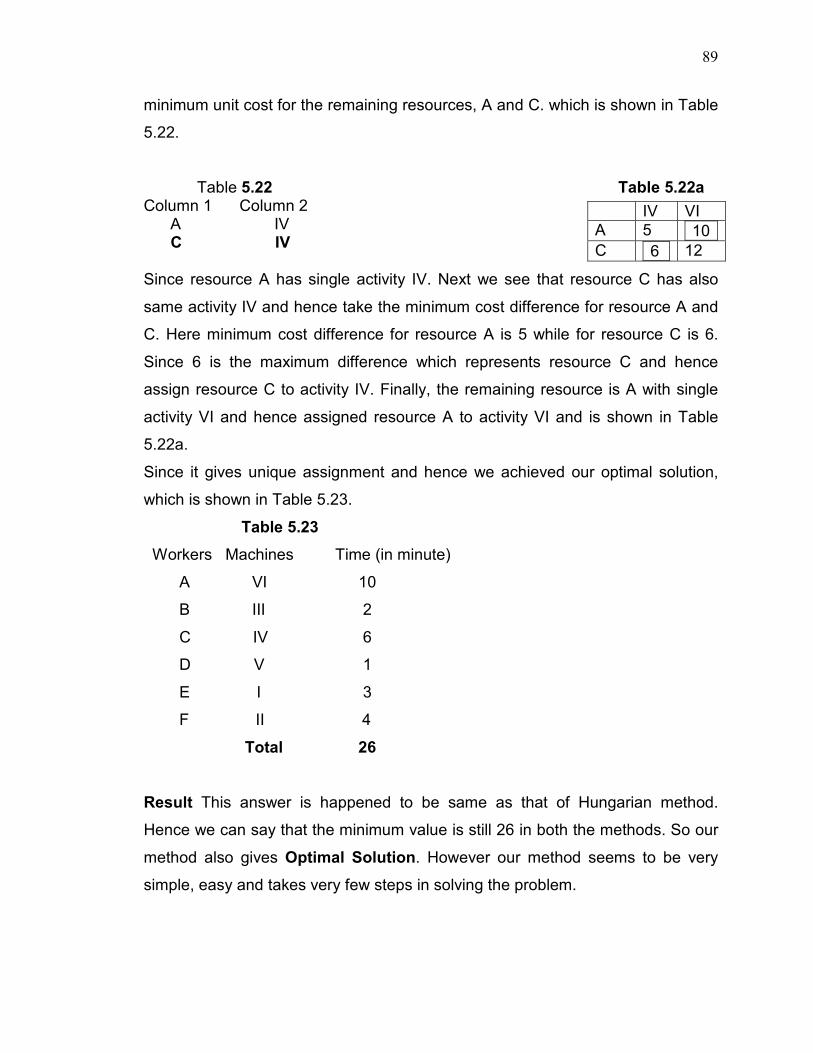
89

minimum unit cost for the remaining resources, A and C. which is shown in Table

5.22.

Table 5.22 Table 5.22a Column 1 Column 2 A IV C IV Since resource A has single activity IV. Next we see that resource C has also

same activity IV and hence take the minimum cost difference for resource A and

C. Here minimum cost difference for resource A is 5 while for resource C is 6.

Since 6 is the maximum difference which represents resource C and hence

assign resource C to activity IV. Finally, the remaining resource is A with single

activity VI and hence assigned resource A to activity VI and is shown in Table

5.22a.

Since it gives unique assignment and hence we achieved our optimal solution,

which is shown in Table 5.23.

Table 5.23

Workers Machines Time (in minute)

A VI 10

B III 2

C IV 6

D V 1

E I 3

F II 4

Total 26


Hence we can say that the minimum value is still 26 in both the methods. So our


simple, easy and takes very few steps in solving the problem.

IV VI A 5 10

C 6

12

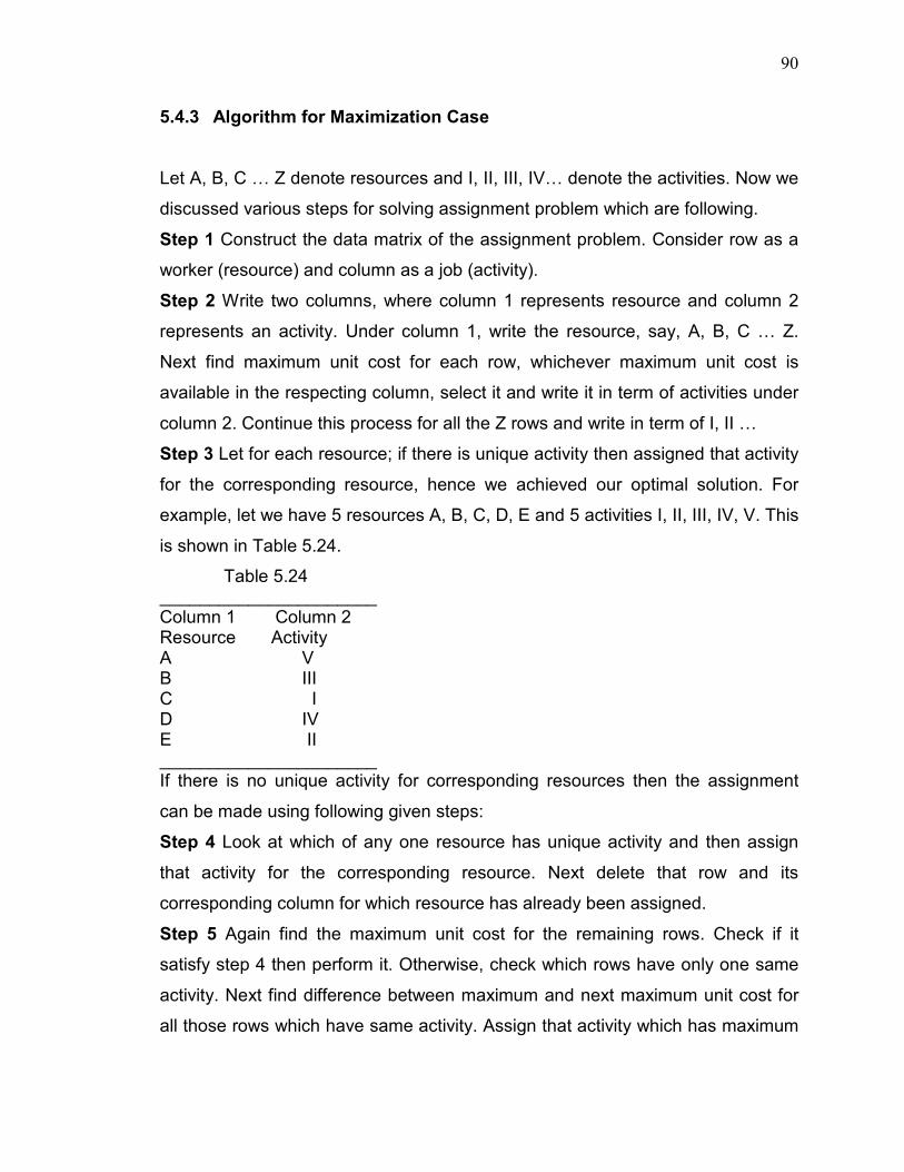
90

5.4.3 Algorithm for Maximization Case

Let A, B, C … Z denote resources and I, II, III, IV… denote the activities. Now we

discussed various steps for solving assignment problem which are following.

Step 1 Construct the data matrix of the assignment problem. Consider row as a

worker (resource) and column as a job (activity).

Step 2 Write two columns, where column 1 represents resource and column 2

represents an activity. Under column 1, write the resource, say, A, B, C … Z.

Next find maximum unit cost for each row, whichever maximum unit cost is

available in the respecting column, select it and write it in term of activities under

column 2. Continue this process for all the Z rows and write in term of I, II …

Step 3 Let for each resource; if there is unique activity then assigned that activity

for the corresponding resource, hence we achieved our optimal solution. For

example, let we have 5 resources A, B, C, D, E and 5 activities I, II, III, IV, V. This

is shown in Table 5.24.

Table 5.24 ______________________ Column 1 Column 2 Resource Activity A V B III C I D IV E II ______________________ If there is no unique activity for corresponding resources then the assignment

can be made using following given steps:

Step 4 Look at which of any one resource has unique activity and then assign

that activity for the corresponding resource. Next delete that row and its

corresponding column for which resource has already been assigned.

Step 5 Again find the maximum unit cost for the remaining rows. Check if it

satisfy step 4 then perform it. Otherwise, check which rows have only one same

activity. Next find difference between maximum and next maximum unit cost for

all those rows which have same activity. Assign that activity which has maximum

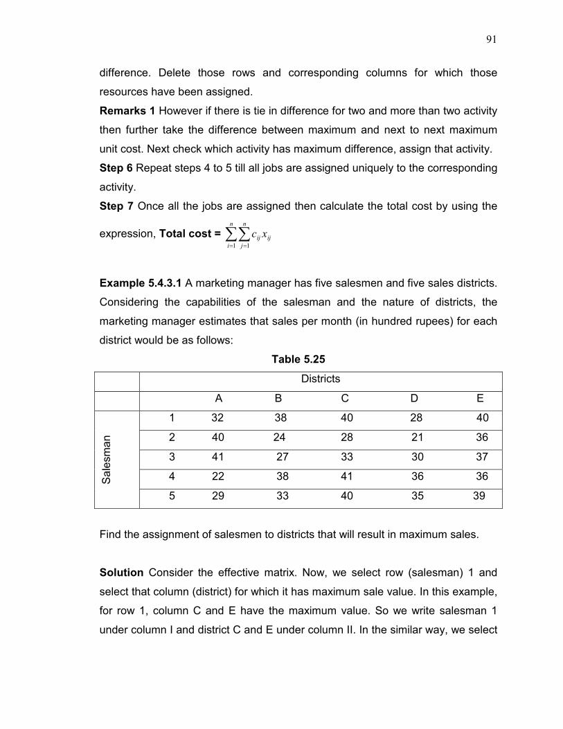
91

difference. Delete those rows and corresponding columns for which those

resources have been assigned.

Remarks 1 However if there is tie in difference for two and more than two activity

then further take the difference between maximum and next to next maximum

unit cost. Next check which activity has maximum difference, assign that activity.

Step 6 Repeat steps 4 to 5 till all jobs are assigned uniquely to the corresponding

activity.

Step 7 Once all the jobs are assigned then calculate the total cost by using the

expression, Total cost = ∑∑= =

n

i

n

j

ijij xc1 1

Example 5.4.3.1 A marketing manager has five salesmen and five sales districts.

Considering the capabilities of the salesman and the nature of districts, the

marketing manager estimates that sales per month (in hundred rupees) for each

district would be as follows:

Table 5.25

Districts

A B C D E

Sales

man

1 32 38 40 28 40

2 40 24 28 21 36

3 41 27 33 30 37

4 22 38 41 36 36

5 29 33 40 35 39

Find the assignment of salesmen to districts that will result in maximum sales.

Solution Consider the effective matrix. Now, we select row (salesman) 1 and

select that column (district) for which it has maximum sale value. In this example,

for row 1, column C and E have the maximum value. So we write salesman 1

under column I and district C and E under column II. In the similar way, we select

92

all the salesmen and find the maximum value for the respective districts, which

are shown in Table 5.26.

Table 5.26 Table 5.26a Resource Activity 1 C, E 2 A 3 A 4 C 5 C

In this example, there is no unique activity for any resource and hence proceed

step 4. The maximum difference between maximum and next maximum profit for

salesman 2 and 3 are 12 and 8 respectively (as for this two resources activity is

same (A)). Here 12 is maximum so assign salesman 2 to district A. This is shown

in Table 5.26a.

Delete salesman 2 and district A. For remaining resources, maximum profit of the

corresponding activity is shown in table 4.27. The maximum difference between

maximum and next maximum profit for salesman 1 and 3 are 0 and 4

respectively (as for this two resources activity is same (E)). Here 4 is maximum

so assign salesman 3 to district E. This is shown in Table 5.27a.


Column 1 Column 2

1 C, E

3 E

4 C

5 C

Delete salesman 3 and district E. For remaining resources, maximum profit of the


maximum and next maximum profit for salesman 1, 4 and 5 are 4, 3 and 5

respectively (as for this two resources activity is same (C)). Here 5 is maximum

so assign salesman 5 to district C. This is shown in Table 5.28a.

A B C D E 1 32 38 40 28 40 2 40

24 28 21 36

3 41 27 33 30 37 4 22 38 41 36 36 5 29 33 40 35 39

B C D E 1 38 40 28 40 3 27 33 30 37

4 38 41 36 36 5 33 40 35 39

93


Column 1 Column 2

1 C

4 C

5 C

Delete salesman 5 and district C. For remaining resources, maximum profit of the


maximum and next maximum profit for salesman 1 and 4 are 10 and 2

respectively (as for this two resources activity is same (B)). Here 10 is maximum

so assign salesman 1 to district B. This is shown in Table 5.29a.


Column 1 Column 2

1 B

4 B

At the last the salesman 4 and district D remains and hence we assign salesman

4 to district D.

Finally, different salesman have assigned district uniquely, which is shown in

Table 5.30.

Table 5.30

Salesman District Sales (in hundred)

1 B 38

2 A 40

3 E 37

4 D 36

5 C 40

Total 191

Result This answer is happened to be same as that of Hungarian method

because the maximum sale value is 191 in both the methods. So our method

also gives Optimal Solution. However our method seems to be very simple,

easy and takes very few steps in solving the problem.

B C D 1 38 40 28 4 38 41 36 5 33 40

35

B D 1 38

28 4 38 36

94

5.4.4 Unbalanced Assignment Problem

The method of assignment discussed above requires that the number of columns

and rows in the assignment matrix be equal. However, when the given cost

matrix is not a square matrix, the assignment problem is called an unbalanced

problem. In such cases a dummy row(s) or column(s) are added in the matrix

(with zeros as the cost elements) to make it a square matrix. For example, when

the given cost matrix is of order 4×3, a dummy column would be added with zero

cost element in that column. After making the given cost matrix a square matrix,

the new alternate method will be used to solve the problem. Once the

unbalanced assignment problem is converted into balanced assignment problem

then we can follow usual algorithm to solve the assignment problem.

Remark Dummy row/column will not be considered for selecting minimum value

in our method for unbalanced assignment problem.

Example 5.4.4.1

A city corporation has decided to carry out road repairs on main four arteries of

the city. The government has agreed to make a special grant of Rs 50 lakh

towards the cost with a condition that the repairs are done at the lowest cost and

quickest time. If the conditions warrant, a supplementary token grant will also be

considered favorably. The corporation has floated tenders and five contractors

have sent in their bids. In order to expedite work, one road will be awarded to

only one contractor.

Table 5.31

Cost of repairs (Rs lakh) R1 R2 R3 R4

Con

trac

tor

s

C1 9 14 19 15 C2 7 17 20 19 C3 9 18 21 18 C4 10 12 18 19 C5 10 15 21 16

Find the best way of assigning the repair work to the contractors and the costs.

95

Solution The given cost matrix is not balanced; hence we add one dummy

column (road, R5) with a zero cost in that column. The cost matrix so obtained is

given in following Table 5.32.

Table 5.32

Cost of repairs (Rs lakh)

R1 R2 R3 R4 R5

Con

trac

tors C1 9 14 19 15 0

C2 7 17 20 19 0

C3 9 18 21 18 0

C4 10 12 18 19 0

C5 10 15 21 16 0

We apply the new alternate method to solve this problem using algorithm

discussed in 5.4.2.

Table 5.33

Column 1 Column 2 Difference

C1 R1 5

C2 R1 10

C3 R1 9

C4 R1 2

C5 R1 5

Assign contractor C2 to repair road R1. Next delete Row C2 and Column R1 and

apply step 4 to 5 which is shown in Table 5.34.

Table 5.34


C1 R2 1

C3 R2, R4 0

C4 R2 6

C5 R2 1



96

Table 5.35


C1 R4 4

C3 R4 3

C5 R4 5



Table 5.36


C1 R3 19

C3 R3 21

In this step, only one column (except dummy column) remains along with two

rows C1 and C3. So assign C1 to R3 (as value is minimum). Next only row C3

remains to assign which will be assign to dummy column R5. Finally each

contractor is assigning to repaired road uniquely which is shown in Table 4.37

along with its corresponding cost.

Table 5.37

Column 1 Column 2 Cost

C1 R3 19

C2 R1 7

C3 R5 0

C4 R2 12

C5 R4 16

Total 54

Result This answer is happened to be same as that of Hungarian method

because the maximum sale value is 54 in both the methods. So our method also

gives Optimal Solution. However our method seems to be very simple, easy

and takes very few steps in solving the problem.

97

Applications Some of the problems where the assignment technique may be

useful are Assignment of workers to machines, salesmen to different sales areas,

clerks to various checkout counters, classes to rooms, etc.

5.5 Conclusion

Hungarian method is used to obtained optimal solution for an assignment

problem. In this chapter, we have developed a new alternate method for solving

an assignment problem where it is shown that this method also gives optimal

solution. Moreover the optimal solution obtained using this method is same as

that of optimal solution obtained by Hungarian method. So we conclude that the

Hungarian method and our method give same optimal solution. However the

technique for solving an assignment problem using our method is more simple

and easy as it takes few steps for the optimal solution.

98

Chapter 6

TRAVELLING SALESMAN PROBLEM

6.1 Introduction

The Traveling Salesman Problem (TSP) is a problem in combinatorial

optimization studied in operations research and theoretical computer science.

Given a list of cities and their pair wise distances, the task is to find a shortest

possible tour that visits each city exactly once.

The problem was first formulated as a mathematical problem by Menger

(1930) and is one of the most intensively studied problems in optimization.

However it was unnoticed till Menger (1994) published a book where he narrated

the foundation of mathematical problem for the travelling salesman problem. It is

used as a benchmark for many optimization methods. Even though the problem

is computationally difficult, a large number of heuristics and exact methods are

known, so that some instances with tens of thousands of cities can be solved.

The TSP has several applications even in its purest formulation, such as

planning, logistics, and the manufacture of microchips. If a slight modification is

made in the problem, it appears as a sub-problem in many areas, such as

genome sequencing. In these applications, the concept city represents, for

example, customers, soldering points, or DNA fragments, and the concept

distance represents traveling times or cost, or a similarity measure between DNA

fragments. In many applications, additional constraints such as limited resources

or time windows make the problem considerably harder. In the theory of

computational complexity, the decision version of TSP belongs to the class of

NP-complete problems. Thus, it is assumed that there is no efficient algorithm for

solving TSP problems. In other words, it is likely that the worst case running time

for any algorithm for TSP increases exponentially with the number of cities, so

99

even some instances with only hundreds of cities will take many CPU years to

solve exactly.

The origins of the traveling salesman problem are unclear. A handbook for

traveling salesmen from 1832 mentions the problem and includes example tours

through Germany and Switzerland, but contains no mathematical treatment.

Hamilton (1800) and Kirkman (1800) expressed the concept of Mathematical

problems related to the travelling salesman problem. The general form of the

TSP appears to have been first studied by mathematicians notably by Menger

(1930). Further Menger (1930) also defines the problem related with salesman

ship based on brute-force algorithm, and observes the non-optimality of the

nearest neighbor heuristic. However Whitney (1930) introduced the name

travelling salesman problem.

During the period 1950 to 1960, the travelling salesman problem started

getting popularity in scientific circle is especially in Europe and the USA. Many

researchers like Dantzig, Fulkerson and Johnson (1954) at the RAND

Corporation in Santa Monica expressed the problem as an integer linear program

and developed the cutting plane method for its solution. With these new methods

they solved an instance with 49 cities to optimality by constructing a tour and

proving that no other tour could be shorter. In the following decades, the problem

was studied by many researchers from mathematics, science, chemistry,

physics, and other sciences. Karp (1972) showed that the Hamiltonian cycle

problem was NP-complete, which implies the NP-hardness of TSP. This supplied

a scientific explanation for the apparent computational difficulty of finding optimal

tours.

6.2 Application of New Alternate Method of Assignment Problem in TSP

We have so far already discussed the algorithm and examples for solving an

assignment problem using a new alternate method in Chapter 5. Now in this

chapter we discuss how the new alternate method for solving an assignment

100

problem can be applied for Travelling Salesman Problem. For this we have

considered an example related with travelling salesman problem and explain in

detail how to find optimal solution using new alternate method of assignment

problem.

Example 6.2.1 A salesman has to visit five cities A.B, C, D and E. The distances

(in hundred kilometers) between the five cities are shown in Table 6.1.

Table 6.1

To city A B C D E

From City

A - 1 6 8 4 B 7 - 8 5 6 C 6 8 - 9 7 D 8 5 9 - 8 E 4 6 7 8 -

If the salesman starts from city A and has to come back to city A, which route

should he select so that total distance traveled become minimum?

Solution

Consider the effective matrix. This is shown in Table 6.2.

Table 6.2

To city A B C D E

From City

A - 1 6 8 4 B 7 - 8 5 6 C 6 8 - 9 7 D 8 5 9 - 8 E 4 6 7 8 -

In this matrix first, we will take first row which is referred a city. We select that

column (assignment) for which it contains minimum distance. For this example,

incase of first row, column B (assignment) has the minimum value. In the similar

way, we select all the rows and find the minimum value for the respective

columns. These are given in Table 6.3.

101

Table 6.3

Column 1(City) Colum 2(Assignment)

A B

B D

C A

D B

E A

In this table, we observed that assignment D occur only once with city B. That is

city B is unique for city D and hence we assign city B to D. This is shown in Table

6.4.

Table 6.4

A B C D E A - 1 6 8 4 B 7 - 8 5

6

C 6 8 - 9 7 D 8 5 9 - 8 E 4 6 7 8 -

However, for other job assignment occur more than once. Hence they are not

unique. So how other job will be assigned further we discuss below.

Next delete row B and column D. Again select minimum cost value for the

remaining cities which is shown below Table 6.5.

Table 6.5


A B

C A

D B

E A

Since assignment B occur with city A and D. Hence first we take the difference

between the value of B and next minimum value (here tie is happens). Here

102

maximum difference is 2 for A and hence we assign B to city A. This is shown in

Table 6.6.

Table 6.6

A B C E A - 1

6 4

C 6 8 - 7 D 8 5 9 8 E 4 6 7 -

Next delete row A and column B. Again select minimum cost value for the


Table 6.7


C A

D A, E

E A

Since assignment A occur with city C, D and E. Hence we take the difference

between the value of A and next minimum value, here the maximum difference is

3 for Job E. And hence we assign A to city E. This is shown in Table 6.8.

Table 6.8

A C E C 6 - 7 D 8 9 8 E 4

7 -

Next delete row E and column A. Again select minimum cost value for the


Table 6.9

Column 1(City) Column 2(Assignment)

C E

D E

103

Here, we cannot assign C to city C. Therefore we only assign E to city C. Then

obviously, we have no other choice rather to assign C for City D.

Finally, we can assign all the cities along with distance which is shown in Table

6.10.

Table 6.10

Column 1(City) Colum 2(Assignment) Distance

A B 1

B D 5

C E 7

D C 9

E A 4

Total 26

This solution is happened to be same as that of Hungarian method. Hence we

can say that the minimum value is still 26 in both the methods. So this solution is

optimal. However our method seems to be very simple, easy and takes very few

steps in solving the method.

6.3 Conclusion

In this chapter, we have applied new alternate method of an assignment problem

for solving Travelling salesman problem where it is shown that this method also

gives optimal solution. Moreover the optimal solution obtained using this method

is same as that of optimal solution obtained by Hungarian method. So we

conclude that the Hungarian method and our method give same optimal solution.

However the technique for solving Travelling Salesman problem using our

method is more simple and easy as it takes few steps for the optimal solution.

104

CHAPTER 7

SUPPLY CHAIN MANAGEMENT

7.1 Introduction

The phrase ‘supply chain management’ appears to have originated in the

early 1980s. Oliver and Webber (1982) discussed the potential benefits of

integrating the internal business functions of purchasing, manufacturing, sales

and distribution. In the modern era, it is a phrase that appears in many

company’s strategies and reports, practitioner and academic journals and texts.

However, there is little consistency in the use of the term and little evidence of

clarity of meaning expressed by Harland (1995a). Rather it appears to be a term

used in several emerging bodies of knowledge which have remained largely

unconnected till to date.

Oliver and Webber (1982), Houlihan (1984), Stevens (1989), Saunders

(1994), Jones and Riley (1985) etc. developed the concept and the meaning of

supply chain management in detail. Ammer (1968) and Lee and Dobler (1965)

explained the pre-existing concepts of Supply Chain Management and found that

It relates closely to materials management. Porter (1985), Johnston and

Lawrence (1988) and Kogut (1985) explained the concepts of Supply Chain

Management in terms of the value of Materials. However, Harland argued that

the supply chain management is concerned with inter business, not intra-

business integration.

There seems to be a universal agreement on what a supply chain is? A

supply chain is a network of autonomous or semi-autonomous business entities

collectively responsible for procurement, manufacturing, and distribution activities

associated with one or more families of related products. A supply chain is a

105

network of facilities that procure raw materials, transform them into intermediate

goods and then finished products, and then finally deliver the products to

customers through a distribution system or a chain. Moreover we can also

express that a supply chain is a network of facilities and distribution options that

performs the functions of procurement of materials. This also transforms these

materials into intermediate and finished products, and finally the distribution of

these finished products to customers.

Next we discuss the supply chain management system using networking in

the following way.

This network is consists of all parties involved directly or indirectly in fulfilling a

customer request.

Figure 7.1

Supply chain can explain with the following example.

Supplier Manufacturer Distributor Retailer CustomerSupplier Manufacturer Distributor Retailer Customer

Supplier Manufacturer Distributor Retailer Customer









Upstream Downstream

106

A manufacturer produced a product which cost is Rs. 1 per product. Now he sells

to the Retailer at a cost of Rs. 6 per product and finally retailer sells to the

customer same product at a cost of Rs. 11 per product.

For this example, we will see the exact profit received by manufacturer

and retailer.

In Supply Chain Management System, any product which is manufactured in a

company, first reaches directly from manufacturer to distributors where

manufacturer sold the product to the distributor with some profit of margin.

Distributors supply that product to retailer with his profit and then finally

customers received that product from retailer. That is called supply chain

management system which implies that a product reaches from manufacturer to

customer through supply. Let manufacturer cost of one product is Rs. 1 and have

produce 1000 such products. Therefore manufacturer cost of 1000 products is

Rs. 1000. Manufacturer supply these products to the distributor at a cost of Rs. 2

per product. Which means that distributor received those products at a cost of

Rs. 2000. So manufacturer’s profit is Rs. 1000. Then retailer received those

products at a cost of Rs. 4 per product from the distributor. That is the retailer

received those product at a cost of Rs. 4000. So distributor’s profit is Rs. 2000.

Finally the customer received these products at a cost of Rs. 7 per product from

the retailer. That is the customer received those products at the cost of Rs. 7000.

So retailer’s profit comes out to be Rs. 3000 only. This shows that customer got

1000 product with a cost of Rs. 5000 more provided customer purchase those

products directly from the manufacturer. To understand this chain we have

developed a mathematical model of Supply of a product from manufacturer-

distributor-retailer-customer. This we discuss in section 7.2.

What is supply chain management?

Supply chain management (SCM) is the combinations of art and science that

goes into improving the way your company finds the raw components it needs to

make a product or service and deliver it to customers. The following are five

basic components of SCM.

107

1. Plan. This is the strategic portion of SCM. Companies need a strategy for

managing all the resources that go toward meeting customer demand for their

product or service. A big piece of SCM planning is developing a set of metrics to

monitor the supply chain so that it is efficient, costs less, and delivers high quality

as well as value to customers.

2. Source. Next, companies must choose suppliers to deliver the goods and

services they need to create their product. Therefore, supply chain managers

must develop a set of pricing, delivery and payment processes with suppliers and

create metrics for monitoring and improving the relationships. And then, SCM

managers can put together processes for managing their goods and services

inventory, including receiving and verifying shipments, transferring them to the

manufacturing facilities and authorizing supplier payments.

3. Make. This is the manufacturing step. Supply chain managers schedule the

activities necessary for production, testing, packaging and preparation for

delivery. This is the most metric-intensive portion of the supply chain where

companies are able to measure quality levels, production output and worker

productivity.

4. Deliver. This is the part that many SCM insiders refer to as logistics, where

company manager coordinate the receipt of orders from customers, develop a

network of warehouses, pick carriers to get products to customers and set up an

invoicing system to receive payments.

5. Return. This can be a problematic part of the supply chain for many

companies. Supply chain planners have to create a responsive and flexible

network for receiving defective and excess products back from their customers

and supporting customers who have problems with delivered products.

Definition

A supply chain is the stream of processes of moving goods from the customer

order through the raw materials stage, supply, production, and distribution of

108

products to the customer. All organizations have supply chains of varying

degrees, depending upon the size of the organization and the type of product

manufactured. These networks obtain supplies and components, change these

materials into finished products and then distribute them to the customer.

Concept of Supply Chain System

Managing the chain of events in this process is known as supply chain

management. Effective management must take into account coordinating all the

different pieces of this chain as quickly as possible without losing any of the

quality or customer satisfaction, while still keeping costs down.

The first step is obtaining a customer order, followed by production, storage and

distribution of products and supplies to the customer site. Customer satisfaction

is paramount. In supply chain process, we are including the customer orders,

order processing, inventory, scheduling, transportation, storage, and customer

service. A necessity in coordinating all these activities is the information service

network.

In addition, key to the success of a supply chain is the speed in which these

activities can be accomplished and the realization that customer needs where

customer satisfaction are the very reasons for the network. Reduced inventories,

lower operating costs, product availability and customer satisfaction are all

benefits which grow out of effective supply chain management.

The decisions associated with supply chain management cover both the long-

term and short-term period. Strategic decisions deal with corporate policies, and

look at overall design and supply chain structure. Operational decisions are those

dealing with every day activities and problems of an organization. These

decisions must take into account the strategic decisions already in place.

Therefore, an organization must structure the supply chain through long-term

analysis and at the same time focus on the day-to-day activities. Manufacturer to

customer will be benefited in real sense if day to day activities are performed.

109

Furthermore, market demands, customer service, transport considerations, and

pricing constraints all must be understood in order to structure the supply chain

effectively. These are all factors, which change constantly and sometimes

unexpectedly. Moreover an organization must realize this fact and be prepared to

structure the supply chain accordingly.

Structure of the supply chain requires an understanding of the demand patterns,

service level requirements, distance considerations, cost elements and other

related factors. It is easy to see that these factors are highly variable in nature

and this variability needs to be considered during the supply chain analysis

process. Moreover, the interplay of these complex considerations could have a

significant bearing on the outcome of the supply chain analysis process.

There are six key elements to a supply chain:

• Production

• Supply

• Inventory

• Location

• Transportation, and

• Information

Application of Supply Chain Management

There are four main uses of the term ‘supply chain management’:

First, the internal supply chain that integrates business functions involved in the

flow of materials and information from inbound to outbound ends of the business.

Secondly, the management of dike or two parties are related with immediate

suppliers. Thirdly, the management of a chain of businesses includes a supplier

and a customer and so on. Fourthly, the management of a network of

interconnected businesses involved in the ultimate provision of product and

service packages required by end customers.

110

Now we develop a mathematical model for Supply Chain Management. In

this model we want to explain how one can find out manufacturer’s price once

the customer price is known. In visa- versa we are also interested to know the

customer price once the manufacturer’s price are known. Such phenomena are

discussed in mathematical model of supply Chain Management developed by us

in section 7.2.

7.2 Mathematical Model of SCM

Let denote price of manufacturer, distributor, retailer and customer by M, D, R

and C respectively. Suppose manufacturer sells his product with more than d1%

of the manufacturer price to the distributor, distributor sells that product with more

than d2% of the distributor price to the retailer. Finally, retailer sells that product

with more than d3% of the retailer price to the customer. We can explain this in

equation form as:

D = M+d1%M (7.1)

R = D+d2%D (7.2)

C = R+d3%R (7.3)

On the basis of the price and the equation provided in (7.1) to (7.3), we

developed a mathematical model to know the price of manufacturer provided

price of customer is known in the following way.

Using (7.3) we can find retailer’s price provided final customer’s price is known in

the following way.

C = R (1+d3)

E.+0.�F � G��1HI� (7.4)

We get price relation between retailer and customer from (7.4).

111

Again using (7.2), we find distributor’s price provided retailer price is known from

(7.4) in the following way.

R = D (1+d2)

J � F�9 2 K3�

On putting the value of R from (7.4), we get D as,

D =

L�MNOI��1HP�

Hence D = G

��1HP�Q��1HI� (7.5)

Now we get price relation between distributor and customer from (7.5).

Finally using (7.1), we can find out manufacturer price provided distributor price

is available from (7.5) in the following way.

D =M (1+d1)

Therefore, M = R

��1HM�

On putting the value of D from (7.5), we get price of Manufacturer as,

M=

L�MNOP�Q�MNOI�

��1HM�

Hence M = G

��1HM�Q��1HP�Q��1HI� (7.6)

Now we get price relation between manufacturer and customer from (7.6).

In visa-versa, we can also find out customer price provided retailer, distributor

and manufacturer price is given along with d1, d2 and d3. This is explained by the

following model.

C=M (1+d1)*(1+d2)*(1+d3) (7.7)

112

From this we found the relation between manufacturer and distributor,

manufacturer and retailer, manufacturer and customer.

Using from (7.7), we have C as,

C=M (1+d1)*(1+d2)*(1+d3)

This relation is between customer and manufacturer.

Putting the value of C in eq. (7.5), we get D as,

D= S��1TM�Q��1TP�Q��1TI�

��1HP�Q��1HI�

Hence we have D=M (1+d1) (7.8)

This relation is between distributor and manufacturer.

Again the putting the value of C in eq. (7.4), we get R as,

R= S��1TM�Q��1TP�Q��1TI�

��1HI�

Finally we have the Price of Retailer as, R= M (1+d1)*(1+d2) (7.9)

This relation is between retailer and manufacturer.

Remark

Using (7.1) to (7.9), one can find price relation of product between customer and

manufacturer, customer and retailer, customer and distributor and visa-versa.

7.2.1 Numeric example Here we demonstrate the price from manufacturer to

customer and vice-versa by a hypothecated numerical example in 7.2.1.1.

Example 7.2.1.1

Manufacturer sold a product with 10% more than the manufacturing price to

distributor, Distributor sold that product with 10% more than the distributor price

to retailer and Retailer sold that product with 35% more than the retailer price to

customer. For this example we have calculated distributor, retailers and customer

price for given manufacturer price.

113

Table 7.1

Manufacturer

price

100

200

300

400

500

600

700

800

900

1000

Solution

Here given is d1=0.10, d2=0.10 and d3=0.35. We have to find distributor, retailers

and customer price for given manufacturer price using (7.8), (7.9) and (7.7).

Table 7.2

M D=M (1+d1) R=M (1+d1)*(1+d2) C=M (1+d1)*(1+d2)*(1+d3) Round figure

Manufacturer Distributor Retailer Customer Customer

price price price price price

100 110 121 163.35 163

200 220 242 326.7 327

300 330 363 490.05 490

400 440 484 653.4 653

500 550 605 816.75 817

600 660 726 980.1 980

700 770 847 1143.45 1143

800 880 968 1306.8 1307

900 990 1089 1470.15 1470

1000 1100 1210 1633.5 1634

Table 7.3

C C/(1+d3) C/(1+d2)*(1+d3) C/(1+d1)*(1+d2)*(1+d3) Round figure

Customer price Retailer price Distributor price Manufacturer price (Manufacturer

Price)

163 120.740741 109.7643098 99.78573615 100

327 242.222222 220.2020202 200.1836547 200

490 362.962963 329.96633 299.9693909 300

653 483.703704 439.7306397 399.755127 400

817 605.185185 550.1683502 500.1530456 500

980 725.925926 659.9326599 599.9387818 600

1143 846.666667 769.6969697 699.7245179 700

1307 968.148148 880.1346801 800.1224365 800

1470 1088.88889 989.8989899 899.9081726 900

1634 1210.37037 1100.3367 1000.306091 1000

114

Remark We also calculated retailer, distributor and manufacturer price by taking

the price of customer obtained in (7.2) in order to check the price of manufacturer

as given in Table (7.2). From Table (7.2) and (7.3), it is clear that the known

manufacturer price in Table (7.2) is same as calculated manufacturer price in

Table (7.3). Similarly known customer price in Table (7.3) is same as calculated

customer price Table (7.2).

7.3 Conclusion

Using this model, if we know customer price and d3 we can find retailer price, if

we know customer price and d2, d3 we can find distributor price, if we know

customer price and d1, d2, d3 we can find manufacturer price and also vice-

versa.

cmehta

Cross-Out

115

CHAPTER 8

CONCLUSIONS AND SCOPE OF FUTURE WORK

8.1 CONCLUSION

In this chapter we discuss the final findings obtained in chapters 3, 4, 5, 6 and 7.

8.1.1 Transportation problem

Chapter 3 deals both the alternate algorithms for a TP as very few alternate

algorithms for obtaining an optimal solution are available in the textbook and in

other literature. These methods are so simple and easy that makes

understandable to a wider spectrum of readers. The methods discussed in

chapter 3, either gives a near optimal solution for certain TP while it gives optimal

solution for other certain TP.

8.1.2 Transshipment Problem

In Chapter 4, we have developed a simple algorithm for solving a Transshipment

Problem. The proposed algorithm is easy to understand and apply. The optimal

solution obtained in this investigation is same as that of MODI method. It will be

possible that basic feasible solution obtained using new alternate method

developed in chapter 4 may yield near to the optimal solution for certain TP

compared to MODI method.

8.1.3 Assignment Problem

So far in the literature Hungarian method is used to obtained optimal solution for

an assignment problem. In chapter 5, we have developed a new alternate

method for solving an assignment problem where it is shown that this method

always gives optimal solution. Moreover the optimal solution obtained using new

alternate method is same as that of optimal solution obtained by Hungarian

method. So we conclude that the Hungarian method and our method give same

116

optimal solution. However the technique for solving an assignment problem using

new alternate method is more simple and easy as it takes few steps for obtaining

the optimal solution.

8.1.4 Travelling Salesman Problem

In chapter 6, we have applied a new alternate method of an assignment problem

for solving Travelling salesman problem where it is shown that this method also

gives optimal solution. Moreover the optimal solution obtained using new

alternate method is same as that of optimal solution obtained by Hungarian

method. So we conclude that the Hungarian method and new alternate method

gives same optimal solution. However the technique for solving travelling

salesman problem based on a new alternate method of assignment problem is

more simple and easy as it takes few steps for the optimal solution.

8.1.5 Supply Chain Management

Using our model discussed in Chapter 7, one can find customer’s price provided

manufacturer’s price is known, similarly manufacturer’s price can be calculated

provided customer’s price is known when value of d1, d2 and d3 are supplied.

8.2 SCOPE OF FUTURE WORK

From chapter 3 to chapter 6, we have developed a new alternate method for

solving Transportation Problem, Transshipment Problem, Assignment Problem

and Travelling Salesmen Problem which gives either near to optimal solution or

optimal solution.

The new alternate methods developed from chapter 3 to 6 are used only for

balanced cases except assignment problem. However we could not made any

attempt to solve unbalanced problem related with transportation and

transshipment problem. Hence one can try to solve unbalanced problem using

new alternate methods developed in this thesis as scope of future work.

117

REFERENCES

1. Adlakha, V. & Kowalski, K. (1999). An Alternative Solution Algorithm for Certain

Transportation Problems, IJMEST 30, 719-728.

2. Adlakha, V. & Kowalski, K. (2009). Alternative Solution Analysis for

Transportation Problems, Journal of Business & Economic Research 11, 41-49.

3. Adlakha, V., Kowalski, K. & Lev, B. (2006). Solving Transportation Problem with

Mixed Constraints, JMSEM 1, 47-52.

4. Ammer, D. S. (1968). Materials Management. Irwin, Homewood, IL, USA.

5. Brezina, I., Cickov, J., Peka, J. & Rei M. (2002). Multi-Stage Transportation

Problem With Capacity Limit. International Journal of Lean Thinking. Volume 1,

42-57.

6. Babbage, C. (1864) Passages from the Life of a Philosopher, London: Longman,

Green, Longman, Roberts, & Green, Chapter 5, page 67. ISBN 1-85196-040-6.

7. Dantzig, G.B (1947). Maximization of a linear function of variables subject to

linear inequalities, T.C. Koopmans (ed.): Activity Analysis of Production and

Allocation, New York-London 1951 (Wiley & Chapman-Hall), pp. 339–347.

8. Dantzig, G. B. (1951). "Application of the Simplex Method to a Transportation

Problem," Activity Analysis of Production and Allocation, Cowles Commission

Monograph 13.

118

9. Dantzig, G. B.; Fulkerson, R.; Johnson, S. M. (1954), "Solution of a large-scale

traveling salesman problem", Operations Research 2 (4): 393–

410, doi:10.1287/opre.2.4.393, JSTOR 166695.

10. Ford, L. R. and Fulkerson, D. R. (1956). “Maximal flow through a network”

Candian Journal of Mathematics 8, 399-404.

11. Garg, R. and Prakash, S. (1985). Time minimizing transshipment problem. Indian

Journal of pure and Applied Mathematics, 1695):449-460.

12. Goyal S. K. (1984). Improving VAM for the Unbalance Transportation Problem, J

Opl Res Soc 35, 1113-1114.

13. Hamilton (1856) Icosian game (marketed in 1859): Find paths and circuits on the

dodecahedral graph, satisfying certain conditions (e.g., adjacency conditions,

etc.).

14. Harland, C. M. (1995a), “The Dynamics of Customer Dissatisfaction in Supply

Chains”, Production Planning and Control, Special Issue on Supply Chain

Management, 6(3), May-June, pp. 209-217.

15. Herer, Y. and Tzur, M. (2001). The dynamic transshipment Problem. Neval

Research Logistics Quarterly, 48, 386-408.

16. Hitchcock, F. L. (1941). "The Distribution of a Product from Several Sources to

Numerous Localities," Journal of Math. and Physics, vol. 20, pp. 224-230.

17. Houlihan, J. (1984). “Supply Chain Management”. Proceedings of 19th

International Technical Conference, BPICS, pp. 101-110.

119

18. JACOBI, C. G. (1890). “De aequationum differentialum systemate non normali ad

formam normalem revocando”, Vorlesungen über Dynamik von C. G. J. Jacobi

nebstes fünf hinterlassenen Abhandlungen desselben, herausegegeben von

A. Clesch, Berlin, Druck und Verlag von Georg Reimer, 1866, p. 550–578 et

C.G.J. Jacobi's gesammelte Werke, fünfter Band, herausgegeben von

K. Weierstrass, Berlin, Druck und Verlag von Georg Reimer, 1890, p. 485-513.

(cf[I/67 a) et b)])

19. Ji Ping & Chu, K. F. (2002). A dual matrix approach to the transportation

problem. Asia-Pacafic Journal of Operations Research, 19, 35-45.

20. Ji Ping, Lee, W. B. & Li Hongyu(1997). A new algorithm for the assignment

problem, An alternative to the Hungarian method. Journal of Computers &

Operations research, 11, 1017-1023.

21. Johnston, R. & Lawrence P. R. (1988). “Beyond Vertical Integration: the Rise of

value adding partnerships”, Harvard Business Review, July- August, pp. 94-101.

22. Jones, T.C. and D. W. Riley (1985). “Using Inventory for Competitive Advantage

through Supply Chain Management”, International Journal of Physical

Distribution and Materials Management, 15(5), pp. 16-26.

23. Judge, G., Havlicek, J. & Rizek, R. (1965). An interregional model: Its formulation

and application to the live stock industry. Agriculture and revision, 7, 1-9.

24. Kantorovich, L.V. (1939). "Mathematical Methods of Organizing and Planning

Production" Management Science, Vol. 6, No. 4 (Jul., 1960), pp. 366–422.

25. Karp, R. M. (1972). “Reducibility Among Combinational Problems”. In R. E. Miller

and J. W. Thatcher, editors, Complexity of computer Computations, pages 85-

103, New York, Plenum Press.

120

26. Khurana, A. and Arora, S. R. (2011). Solving Transshipment Problem with mixed

constraints. International journal of Management Science and Engineering

Management. 6(4):292-297.

27. King, G. and Logan, S. (1964). Optimal location, number, and size of processing

plants with raw product and final product shipment. Journal of Farm Economics,

46:94-108.

28. Kirkman (1856), rector of the parish of Craft with Southworth, Lancashire, from

1840 to 1892. Philosophical Transactions of the Royal Society, London, 146

413–418.

29. Kogut, B. (1985). : Designing Global Strategies: Comparative and Competitive

value added chains”, Sloan Management Review, Summer, pp. 15-28.

30. Konig, D. (1931). Graphok es matrixok [in Hungarian: Graphs and matrices], Mat

es Fizikai Lapok 38, 116-119.

31. Koopmans T. C. (1949). Optimum utilization of the transportation system.

Econometrica, 17, 3-4.

32. Korda, B.( 1967). Matematické metódy v ekonómii. Praha: SNTL - Nakladatelství

technické literatury,

33. Kuhn, H. W. (1955). “The Hungarian Method for the assignment problem”, Naval

Research Logistics Quarterly, Kuhn’s original publication, 2, 83-97.

34. Lanchest, F.W.(1956). Mathematics in Warfare in the World of Mathematics, Vol.

4 Ed. Newman, J.R., Simon and Schuster, 2138-2157.

35. Lee, L. and Dobler D. (1965). Purchasing and Materials Management, McGraw-

Hill, New York, USA.

121

36. Li Wu Ji & Smith J. MacGregor(1995). An algorithm for Quadratic Assignment

Problems. European journal of Operations Research, 1, 205-216.

37. Menger, K. (1994). “Reminiscences of the Vienna circle and the Mathematical

Colloquium”. Dortmund.

38. Munkres, J. (1957). “Algorithms for the Assignment and Transportation

Problems”, Journal of the Society for Industrial and Applied Mathematics, 5(1),

32-38.

39. Neumann, J. V. & Morgenstern, O. (1944). Theory of Games and Economic

Behavior, Princeton University Press.

40. Oliver, R. k. and Webber, M. D. (1982). “Supply Chain Management: Logistics

Catches Up With Strategy”. In: M. Christopher (1992), Logistics: The Strategic

Issues, pp. 63-75. Chapman and Hall, London, UK.

41. Orden, A. (1956). Transshipment problem. Management science, 3:276-285.

42. Porter, M. E. (1985). Competitive Advantages: Creating and Sustaining superior

Performance. Free Press, New York, USA.

43. Ramakrishnan, C. S. (1988). An Improvement to Goyal’s Modified VAM for the

Unbalanced Transportaion Problem, J Opl Res Soc 39, 609-610.

44. Rhody, D. (1963). Interregional competitive position of the hog-pork industry in

the southeast United States. Ph.D. thesis, Iowa State University.

45. Saunders, M. (1994). Strategic Purchasing and Supply Chain Management.

Pitman, London, UK.

122

46. Sharma J K. Q uantitative Techniques(2007). (6th ed.). New Delhi: Macmillan.

47. Stevens, G. C. (1989). “Integrating the Supply Chain”, International Journal of

Physical Distribution and Materials Management, 19(8), pp. 197-208.

48. Sultan, A. & Goyal, S.K. (1988). Resolution of Degeneracy in Transportation

Problems, J Opl Res Soc 39, 411-413.

49. Sultan, A. (1988). Heuristic for Finding an Initial B. F. S. in Transportation

Problems, Opsearch 25, 197-199.

50. Thompson Gerald L. (1981). A recursive method for solving assignment problem.

Journal of Science Direct- North-Holland Mathematics Studies, 59, 319-343.

51. Tolsto, A.N. (1930). Metody nakhozhdeniya naimen’shego summovogo

kilometrazha pri planirovanii perevozok v prostranstve [Russian; Methods of

finding the minimal total kilometrage in cargotransportation planning in space]. In:

Planirovanie Perevozok, Sbornik pervy˘ı [Russian; Transportation Planning,

Volume I], Transpechat’ NKPS [TransPress of the National Commissariat of

Transportation], Moscow, pp. 23–55.

52. Tomizawa, S. (1990b). Polynomial diagonals-parameter symmetry model for

square contingency tables with ordered categories, statistics, 50, 171-178.

53. www.charlesbabbage.net

54. en.wikipedia.org/wiki/operations_research

55. www.phpsimplex.com/en/history/htm

saurashtra universityetheses.saurashtrauniversity.edu/916/1/gilani_ms_thesis_statistics.pdfdoctor of...

Documents