Satellite Altimetry andSatellite Altimetry andGravimetryGravimetry: : Theory and ApplicationsTheory and Applications

C.K. ShumC.K. Shum1,21,2, Alexander Bruan, Alexander Bruan2,12,1

1,21,2Laboratory for Space Geodesy & Remote SensingLaboratory for Space Geodesy & Remote Sensing 2,12,1Byrd Polar Research CenterByrd Polar Research Center

The Ohio State UniversityThe Ohio State UniversityColumbus, Ohio, USAColumbus, Ohio, USA

ckshum@osu.ckshum@osu.eduedu, , braunbraun.118@.118@osuosu..edueduhttp://geodesy.eng.ohio-state.http://geodesy.eng.ohio-state.eduedu

Norwegian Univ. of Science and TechnologyTrondheimTrondheim, Norway, Norway

2121––25 June, 200425 June, 2004

Satellite Altimetry andSatellite Altimetry and Gravimetry Gravimetry::Theory and ApplicationsTheory and Applications

Thursday, 24 June 2004Thursday, 24 June 2004

•• Ocean Tides Determination from Satellite AltimetryOcean Tides Determination from Satellite Altimetry (AM) C.K.(AM) C.K.ShumShum

•• Temporal Gravity Field Observations with GRACETemporal Gravity Field Observations with GRACE (AM) C.K.(AM) C.K.ShumShum

•• IceSat IceSat Research and ApplicationsResearch and Applications (PM) Alexander Braun(PM) Alexander Braun

Ocean Tides DeterminationOcean Tides Determinationfrom Satellite Altimetryfrom Satellite Altimetry

C.K. Shum, C.K. Shum, Yuchan Yuchan YiYiLaboratory for Space Geodesy & Remote SensingLaboratory for Space Geodesy & Remote Sensing

The Ohio State UniversityThe Ohio State UniversityNorwegian Univ. of Science and Technology

TrondheimTrondheim, Norway, Norway2121––25 June, 200425 June, 2004

Introduction to Tides

OCEAN TIDESOCEAN TIDES• Tides have been important for for commerce and science for at least 4,000 years (interdisciplinary science)• Tides produce currents, change the length of day, cause the moon to keep one face towards the Earth, influence almost all precise measurements of the Earth• During the last 4,000 years, greatest scientists have tried to understand, calculate and predict tides: Galileo, Descartes, Kepler, Newton, Euler (1740), Bernoulli (1740), Kant (1754), Laplace (1775), Airy (1845), Lord Kelvin (1872), Jeffereys (1923), Munk (1951), Cartwright (1960).

Key Questions: What is the amplitude and phase of theKey Questions: What is the amplitude and phase of thetides at any place on the ocean? What is the shape oftides at any place on the ocean? What is the shape ofthe tides? How and where are tides dissipate?the tides? How and where are tides dissipate?

Topography-Trapped Tides: Topography-Trapped Tides: Awaji Awaji Is, JapanIs, Japan

JapanJapan•

Movie credit: BillMovie credit: BillPichel Pichel (2004)(2004)

Tidal Coupling/Locking of Earth & MoonTidal Coupling/Locking of Earth & Moon

• The Moon has a rotational period of 27.3 days that(except for small fluctuations) exactly coincides withits (sidereal) period for revolution about the Earth -Tidal Locking of the periods for revolution androtation - Moon keeps the face turned towards theEarth

The “Far Side” (or the “Dark Side”) of the Moon

Lunar DecelerationLunar Deceleration• Space geodetic technique (lunar and satellite laser ranging)determined deceleration of the Moon’s mean motion and theattendant decrease in the Earth’s rotation rate are results of tidaldissipation in the ocean and solid Earth [e.g., Cheng et al., 1992].Cheng et al. [1992] provided an estimate of lunar deceleration at–25.25±0.4 arcs/century2

• Billions year later, the Earth will slow down its rotation to have theexact period as the Moon’s

• Length of Day rate ≈ +0.025 ms/yr or increase of 2.5 ms/century

Tide-generating forceon the surface of the earth

Fc

Fc

A(O)O

A(X)

For each celestial body attracting the earth,F(X), the force driving the ocean water at alocation X is a vector sum ofA(X), gravitational attraction of the body, andFc, centrifugal force due to earth’s orbital motion: F(X) = A(X) + Fc = A(X) – A(O)O is the center of the earth.

(to attracting body)

X

F(X) varies periodically in time asthe earth’s orbital motion does

Equilibrium Ocean TidesEquilibrium Ocean TidesEquilibrium tides (lunar or solar) is thetheoretical ocean tidal response for:• Spherical Earth totally covered by ocean• Ocean depth is unifrom with uniform water density• Frictionless ocean, instantaneous ocean response to gravitational forces (no ‘inertia’, no ‘ocean dynamics’, ocean loading, etc)

Equilibrium tides quite different from real tides, however,Equilibrium tides quite different from real tides, however,with same temporal characteristics (known with same temporal characteristics (known ‘‘frequenciesfrequencies’’))and manifest in the tidal potential which is used to forceand manifest in the tidal potential which is used to forcemodels, and compute satellite orbit perturbationsmodels, and compute satellite orbit perturbations

Woodworth [2002]Woodworth [2002]

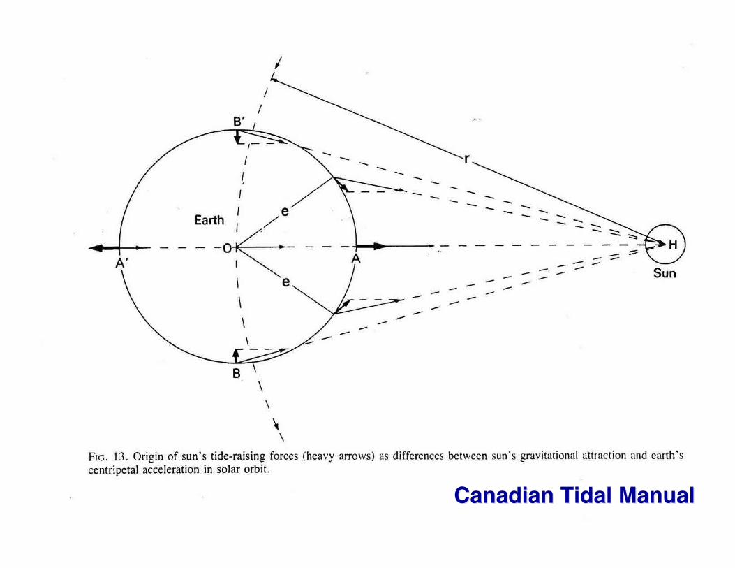
Canadian Tidal ManualCanadian Tidal Manual

TidesSolid Earth tides, (geocentric) ocean tides, pole tides Ocean Tides Using FES94 Model

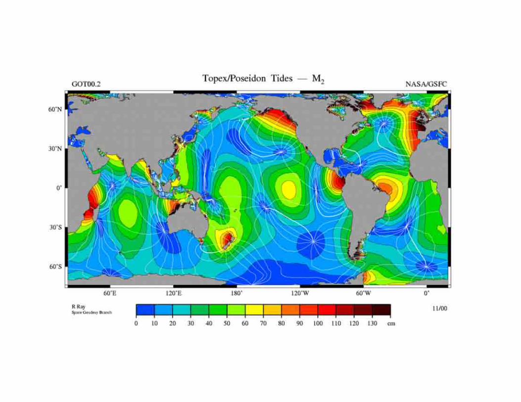
BAROTROPIC OCEAN TIDES BASED ONBAROTROPIC OCEAN TIDES BASED ONMM22, S, S22, K, K11, AND O, AND O11 CONSTITUENTS CONSTITUENTS

Movie covers 4 days beginning at 1 Jan, 1992, 0 hr with 30 minute frames

CSR3.0 Model[Eanes, 1995]Movie credit:C. Tierney

€

˙ ̇ r = −µr r3

← vector← scalar

+ ∇U + F

Equation of Motion:

U - conservative (gravitational) forcesF - Non-conservative forces

€

U(r ,φ ,λ,t) =GMe

ae

ae

r

m =0

l

∑l =1

∞

∑l+1

P lm(sinφ ) C lm(t)cosmλ+ S lm(t)sinmλ[ ]

€

ΔUst =GMe

ae2 Hk

k (l,m )∑ ei (Θ k+ χ k )kk

0

m=0

l

∑l=2

(3)

∑ aer

l+1

Yml (φ ,λ)+ kk

+ aer

l+ 3

Yml+ 2(φ ,λ)

€

ΔUot = 4πGρwae1+ k ' l2l+1+

−

∑m=0

l

∑l=0

∞

∑k∑ ae

r

l+1

Cklm± cos(Θ k ±mλ)+ Sklm

± sin(Θ k ±mλ)[ ]Plm(sinφ )

Geopotential, earth tide, ocean tide potentials:

GLOBAL OCEAN TIDE MODELS• Model availability

JPL/PODAAC: http://podaac.jpl.nasa.gov NASA/GSFC: http://bowie.gsfc.nasa.gov/926/ NAO, Japan: http://www.miz.nao.ac.jp CNES/GRGS: http://www.omp.obs-mip.fr/omp/legos

• Model Evaluations

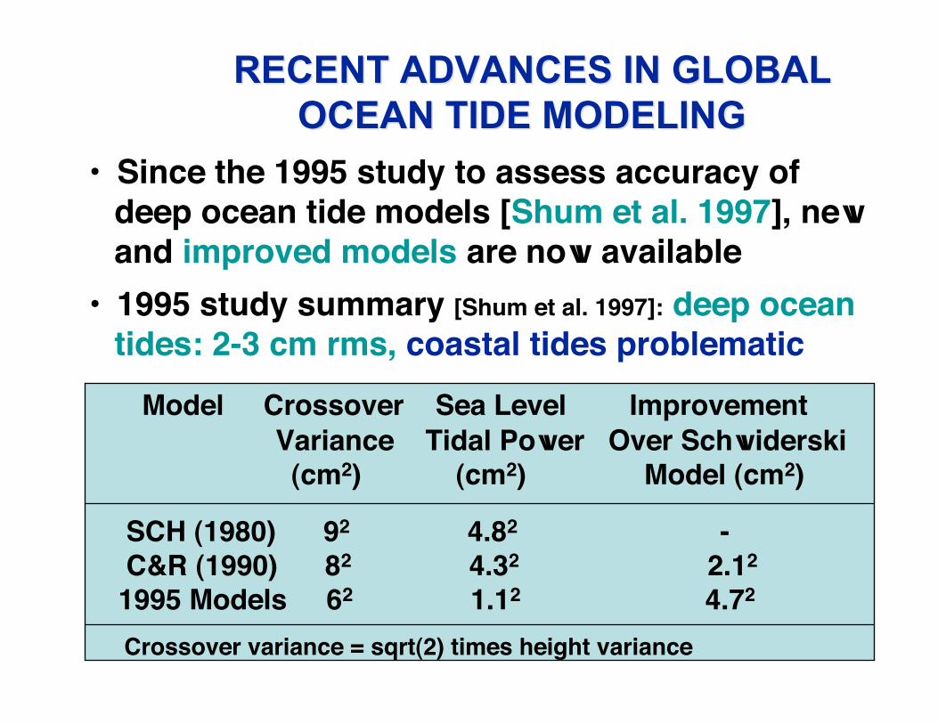
RECENT ADVANCES IN GLOBAL RECENT ADVANCES IN GLOBAL OCEAN TIDE MODELING OCEAN TIDE MODELING

• Since the 1995 study to assess accuracy of deep ocean tide models [Shum et al. 1997], new and improved models are now available• 1995 study summary [Shum et al. 1997]: deep ocean tides: 2-3 cm rms, coastal tides problematic Model Crossover Sea Level Improvement Variance Tidal Power Over Schwiderski (cm2) (cm2) Model (cm2)

SCH (1980) 92 4.82 - C&R (1990) 82 4.32 2.12

1995 Models 62 1.12 4.72

Crossover variance = sqrt(2) times height variance

RECENT GLOBAL OCEAN TIDE MODELSRECENT GLOBAL OCEAN TIDE MODELS•• 1994/1995 global ocean models (over 10) used in the 19951994/1995 global ocean models (over 10) used in the 1995

tide model study [Shum et al. 1997] tide model study [Shum et al. 1997] (JPL CD-ROM product)(JPL CD-ROM product)•• Examples ofExamples of 1999 global ocean tide models (over 8):1999 global ocean tide models (over 8):

• YATM4d (Tierney et al. Univ. of Colorado, assimilatedmodel)

• Arthur Smith (Delft Tech. Univ. empirical model)• TPX0.3 (G. Egbert, Oregon St. U. deep ocean assimil.

model)• D&W98 (Desai & Wahr, JPL/CU deep ocean empirical

Model)• CSR4.0 (R. Eanes, Univ. of Texas empirical model)• GOT99.2b (R. Ray, NASA/GSFC empirical/patched model)• NAO99 (K. Matsumoto, Nat. Astron. Obs. assimilated

model)• FES99 (C. LeProvost, LEGOS/GRGS assimilated model)

•• 2000 or later models: FES00, GOT002000 or later models: FES00, GOT00

ACCURACY ASSESSMENT OF OCEANACCURACY ASSESSMENT OF OCEANTIDE MODELS IN COASTAL REGIONSTIDE MODELS IN COASTAL REGIONS

• Assess present knowledge of coastal tide– Compute rss vector tidal height standard deviations between 6

current selected models (vector differences summed for 8 majorconstituents) as estimated errors

• Evaluation using altimeter sea level data– Assess coastal tide error using altimeter sea level data

computed using altimetric SSH subtracting a mean seasurface (OSUMSS95, Yi and Rapp, [1995])

– Use independent and improved altimeter data [Shum et al.1999, Urban et al. 1999]:

• TOPEX/POSEIDON (1999), ERS-1 Phase E&F(1994-1995, Geodetic Phase), and Geosat GeodeticMission and Exact Repeat Mission (1985-1987) data

• Evaluation using pelagic and coastal tidegauge data

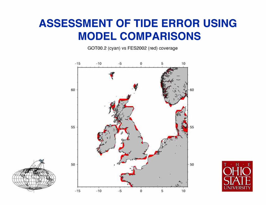
ASSESSMENT OF TIDE ERROR USINGASSESSMENT OF TIDE ERROR USINGMODEL COMPARISONSMODEL COMPARISONS

ASSESSMENT OF TIDE ERROR USINGASSESSMENT OF TIDE ERROR USINGMODEL COMPARISONSMODEL COMPARISONS

Deep Ocean: depth > 1000 mCoastal Ocean: depth < 1000 m Shum et al. [2001]

Estimated Tide Errors (rms):Deep ocean: 2.4 cmCoastal ocean: 2.4 cm to 293.21 cm Maximum

Yellow Sea: 36.58 cm 150.42 cmIndonesian Sea: 14.22 cm 99.11 cmPatagonian Shelf: 19.15 cm 99.70 cmGulf of Mexico: 4.69 cm 49.77 cm

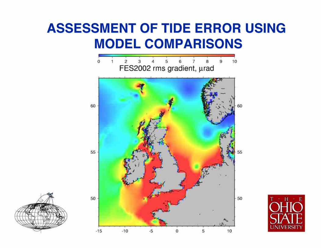
ASSESSMENT OF TIDE ERROR USING ASSESSMENT OF TIDE ERROR USING MODEL COMPARISONSMODEL COMPARISONS

ASSESSMENT OF TIDE ERROR USING ASSESSMENT OF TIDE ERROR USING MODEL COMPARISONSMODEL COMPARISONS

ASSESSMENT OF TIDE ERROR USING ASSESSMENT OF TIDE ERROR USING MODEL COMPARISONSMODEL COMPARISONS

ASSESSMENT OF TIDE ERROR USING ASSESSMENT OF TIDE ERROR USING MODEL COMPARISONSMODEL COMPARISONS

ASSESSMENT OF TIDE ERROR USING ASSESSMENT OF TIDE ERROR USING MODEL COMPARISONSMODEL COMPARISONS

ASSESSMENT OF TIDE ERROR USING ASSESSMENT OF TIDE ERROR USING MODEL COMPARISONSMODEL COMPARISONS

TIDE MODEL EVALUATIONS USINGTIDE MODEL EVALUATIONS USINGTOPEX/POSEIDON SEA LEVELTOPEX/POSEIDON SEA LEVEL

Coastal Ocean (depth<1000m) T/P Sea Level Residual rms (cm) in Regions

Tide models I II III IV V VICSR3.0 14.10 22.16 21.83 23.38 18.72 12.29YATM4d 19.04 31.53 38.06 37.48 23.71 21.62CSR4.0 12.73 19.38 19.33 19.13 17.93 11.70GOT99.2 11.01 17.09 18.82 17.91 16.46 11.50NAO99 10.17 16.32 17.44 15.85 17.57 11.63Smith 18.39 40.51 29.87 34.61 33.54 15.03

I Gulf of Mexico II South America III Gulf of Alaska IV China Sea V North Sea VI Africa

• Sea Level = Altimeter SSH - OSUMSS95 • Latitude weights applied • Edit criteria = 1000cm

TIDE MODEL EVALUATIONS USINGTIDE MODEL EVALUATIONS USINGTOPEX/POSEIDON SEA LEVELTOPEX/POSEIDON SEA LEVEL

Coastal Ocean (depth<1000m)

T/P Sea Level Residual rms (cm) in RegionsTide models Yellow sea Indonesia S. America N. America CSR3.0 33.78 21.21 26.38 6.76 YATM4d 39.07 35.57 30.01 26.60 CSR4.0 25.81 16.99 21.76 6.75GOT99.2 22.23 15.83 20.34 5.64 NAO99 17.75 14.24 17.86 6.68 Smith 50.63 30.34 51.13 9.60

• Sea Level = Altimeter SSH - OSUMSS95 • Latitude weights applied

• Edit criteria = 1000 cm

TIDE MODEL EVALUATIONS USINGTIDE MODEL EVALUATIONS USINGALTIMETER SEA LEVELALTIMETER SEA LEVEL

Global coastal ocean (depth<1000m)

GEOSAT (Residualrms, cm)

Tide Models GM ERM ERS-1 T/P CSR3.0 52.59 111.04 26.72 21.53 YATM4d 58.43 110.96 34.60 33.56 CSR4.0 51.96 53.99 25.40 19.09 GOT99.2 46.96 48.53 25.15 17.75 NAO99 51.90 53.67 24.70 17.04 Smith 47.97 47.51 32.37 33.28

• Sea Level = Altimeter SSH - OSUMSS95• Latitude weights applied [Yi and Rapp, 1995]• Edit criteria = 1000 cm

TIDE MODEL EVALUATIONS USINGTIDE MODEL EVALUATIONS USING102 PELAGIC TIDE GAUGES102 PELAGIC TIDE GAUGES

M2 K2 N2 S2 K1 O1 P1 Q1 RSS CSR3.0 1.75 0.52 0.66 1.11 1.15 0.92 0.40 0.29 2.72 YATM4d 1.40 0.44 0.57 0.91 1.21 0.84 0.39 0.26 2.39 CSR4.0 1.67 0.50 0.64 1.07 1.11 0.88 0.39 0.32 2.62GOT99.2 1.44 0.42 0.64 0.99 1.03 0.84 0.35 0.27 2.37 NAO99 1.64 0.44 0.67 1.10 1.16 0.86 0.37 0.25 2.61

• YATM4d model has assimilated tide gauge data • Amospheric tide inconsistency not corrected [Ray, 1995]

TIDE MODEL EVALUATIONS USINGTIDE MODEL EVALUATIONS USING739 COASTAL TIDE GAUGES739 COASTAL TIDE GAUGES

M2 K2 N2 S2 K1 O1 P1 Q1RSS

CSR3.0 20.59 2.11 4.18 7.30 5.94 3.71 1.85 0.74 23.50 YATM4d 20.61 2.13 4.08 7.48 5.92 3.86 1.79 0.72 23.57 CSR4.0 19.89 2.05 4.04 7.09 5.92 3.52 1.86 0.70 22.75GOT99.2 13.72 1.63 2.99 5.27 4.23 2.53 1.34 0.57 15.94 NAO99

• YATM4d model has assimilated tide gauge data • Amospheric tide inconsistency not corrected [Ray, 1995]

ASSESSMENT OF TIDE ERROR USINGASSESSMENT OF TIDE ERROR USINGMODEL COMPARISONSMODEL COMPARISONS

1 µrad = 1 cm over 10 km

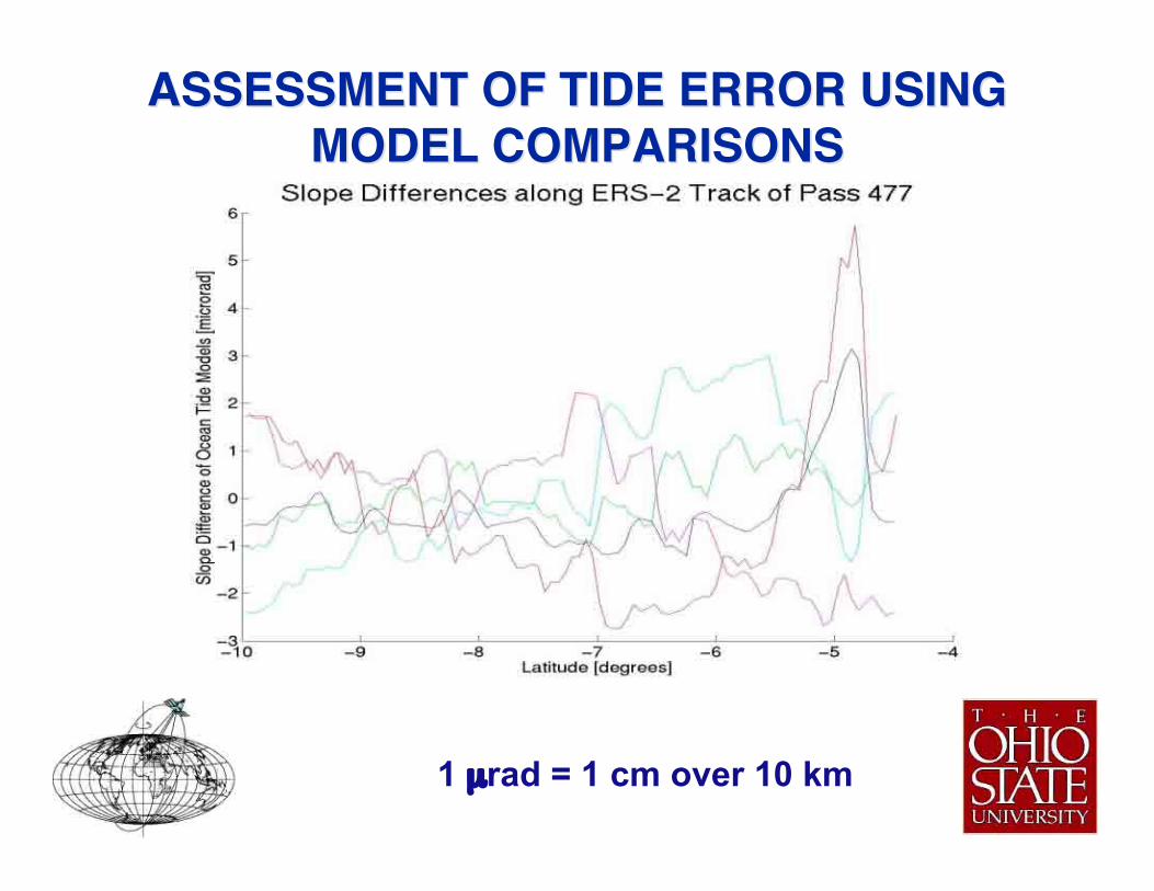
ASSESSMENT OF TIDE ERROR USINGASSESSMENT OF TIDE ERROR USINGMODEL COMPARISONSMODEL COMPARISONS

1 µrad = 1 cm over 10 km

Tidal Aliasing and AltimetricOrbit Design

Aliasing caused by Slow Sampling

Sampling Period TA Remote Sensing Satellite flies over the same locationperiodically at every several days, for example, T = 9.9 days“sample” for T/P Satellite

Tidal Periods TkMost strong tidal signals have periods close to 1 or 0.5day/cycle, much shorter than the sampling Period ofsatellites, i.e., Tk < T

Aliased Tidal Period TakThis slow sampling makes the observed tidal signalindistinguishable from that with a longer Aliased Period Tak

> T (> Tk)

Need to select T so that Tak’s are well separated

•• Sampling a signal with a longer period causesSampling a signal with a longer period causesaliasing effectaliasing effect

M2 Tide Sampled Once per 9.9 Days

For T = 9.9 days of TOPEX/POSEIDON,Tk = 0.52 days/cycle Tak = 62.1 days/cycle

Tidal Aliasing Periods (Days) for Ocean Tides From Satellite Altimeters

Tides Geosat/GFO ERS/Envisat T/P/Jason Space Station

M2 317 95 62 9.89

S2 169 ∞ 59 29.99

N2 52 97 50 7.28

K2 88 183 87 35.88

O1 113 75 46 11.48

P1 4466 365 89 51.52

K1 176 365 173 71.76

Q1 74 133 69 8.10

Mm 45 130 28

Mf 69 -80 36

Ssa 183 183 183

Aliased frequencyfa = ABS[mod(fk+fN, 2fN) - fN]

where fN= 1/2T Nyquist frequency

Example for Topex/POSEIDON (T=9.9156 days)fk = 1/0.5175 days to fa = 1/62.11 days for M2

fk = 1/0.5 days to fa = 1/58.74 days for S2

Coverage:T/P ~ ±660

GFO ~ ±720

ERS ~ ±660

[ 4 ] Analysis, determined results

Ocean Tide Solution Techniques: • Harmonic analysis • Orthotide analysis [Cartwright, 1966] • Harmonic or orthotide analysis using (hydrodynamic) model (tide gauge and/or altimeter) data assimilations [Matsumoto et al., 2001]• Note: First two techniques assumes mostly linear admittance property of tidal constituents, might have problems in coastal regions

Earth Satellite Altimetry MissionsEarth Satellite Altimetry Missions

PlannedPlanned:: CRYOSAT (2004), JASON-2 (2006) CRYOSAT (2004), JASON-2 (2006)ProposedProposed:: ABYSS, NPOESS, GAMBLE ABYSS, NPOESS, GAMBLE

2003ICESAT (laser)

2002ENVISAT

2001JASON

1998GFO

1995ERS-2

1992TOPEX/POSEIDON

1991ERS-1

1984GEOSAT

1978SeaSat

1974GEOS 31973Skylab

Launch DateMission

74.050132.80669.365Q1

87.724182.62186.596K2

4466.665365.24288.891P1

52.07297.39349.528N2

112.95475.06745.714O1

175.448365.242173.192K1

168.817°fi58.742S2

317.10894.48662.107M2

17.05 daysGeosat/GFOrepeat orbit

35 days ERS-1/2repeat orbit

9.9days T/Prepeat orbit

Aliased Period (days/cycle)

Tidalharmonics

Aliased period of 8 major tidal constituents by periodicaltimiter sampling

Analysis model of ocean tide

Fourier series for periodic functions ζ(t, X) = Σk Hk(X) cos[εk +2πfkt - Gk(X)]

ζ(t, X): tidal height at time t and a point X

fk, εk: astronomic constants (global)

Hk(X), Gk(X): harmonic constants at a point X

Harmonic constants change with location because responseof sea height and current to the tide-generating force dependson ocean depth and friction at sea floor. They need to bedetermined based on measurements like tide gauge data and

satellite altimeter data.

Rayleigh Criterion of Harmonic Data Analysis to separate two neighboring tidal frequencies f1 and f2, total time span _t of data record should be long enough so that 1/_t < |f1-f2|, fk =1/Tak

Convolution Theorem of Linear Dynamic Systems G(fk) = H(fk)F(fk) in the Frequency Domain for frequency fk G(fk) is Fourier transform of tidal height (ocean response) F(fk) corresponds to tide-generating potential (driving force) H(fk) - Admittance, Fourier transform of Response Function

Response Method of Parameter Estimation Admittance Function H(fk), a smooth function of frequency requiring a small number of weight parameters (orthotide)⇒ estimability of unknown weight parameters is independent of Rayleigh criterion in principle (shorter data span!)

Response Analysis at a Point

Sea Surface Height (SSH) Data above a Ref. Ellipsoid After correcting for instrument corrections, radar path delays, sea-state bias, atm. pressure loading, solid earth tide, and pole tide,

SSH = N + ODT + elastic ocean tidal height

N is geoid undulation and ODT is ocean dynamic topography

Full or Residual Ocean Tide Solution Full Solution- Direct Harmonic Data Analysis of SSH without Initial Ocean Tide Model

Residual Solution – Improve an Initial Ocean Tide Model Using residual SSH Data

SSH Data at Single/Dual Satellite Crossover Points Unevenly time-sampled data containing harmonic information at additional phase (Single-) or two sampling rates (Dual Sat.)

Satellite Radar Altimeter (RA) Observables

Rayleigh Criterion of Harmonic Data Analysis to separate two neighboring tidal frequencies f1 and f2, total time span _t of data record should be long enough so that 1/_t < |f1-f2|, fk =1/Tak

Convolution Theorem of Linear Dynamic Systems G(fk) = H(fk)F(fk) in the Frequency Domain for frequency fk G(fk) is Fourier transform of tidal height (ocean response) F(fk) corresponds to tide-generating potential (driving force) H(fk) - Admittance, Fourier transform of Response Function

Response Method of Parameter Estimation Admittance Function H(fk), a smooth function of frequency requiring a small number of weight parameters (orthotide)⇒ estimability of unknown weight parameters is independent of Rayleigh criterion in principle (shorter data span!)

Response Analysis at a Point

Ocean tide modeling : Response method

[ ]

[ ] nbiastwatwa

tQvtPutZ

iiiii

m kkkkk

++++

+=

∑

∑∑= =

)sin(),()cos(),(

)(),()(),(),,(

21

2

1

2

0

ϕλϕλ

ϕλϕλϕλ

:)(),( tQtP kk Orthotide function

:),(),,( ϕλϕλ kk vu Coefficients of orthotide function

Due to the aliasing problem in harmonic analysis, we use responsemethod with Orthotide formula (Grove and Reynolds,1975;Andersen, 1995)

(1)

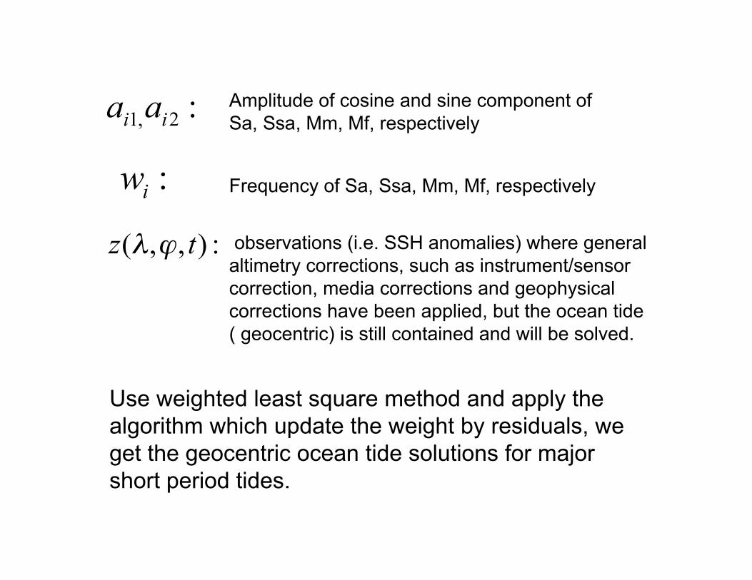
:2,1 ii aa Amplitude of cosine and sine component ofSa, Ssa, Mm, Mf, respectively

:iw Frequency of Sa, Ssa, Mm, Mf, respectively

:),,( tz ϕλ observations (i.e. SSH anomalies) where generalaltimetry corrections, such as instrument/sensorcorrection, media corrections and geophysicalcorrections have been applied, but the ocean tide( geocentric) is still contained and will be solved.

Use weighted least square method and apply thealgorithm which update the weight by residuals, weget the geocentric ocean tide solutions for majorshort period tides.

Th

hT

uT

uAZuAZN

C

ZCACACAu

nAuZ

h

)~)(~(1ˆ

ˆ)ˆ(~ 1111

−−=

+=

+=−−−−

Algorithm for weighting (Tapley, 1971; Anderson, 1995)

is the variance of the observations, here we assume 3cmerror for Topex measurement and 8cm error for ERS2measurement as a priori accuracy.

hC

uCis the variance of the coefficient of the orthotidefunctions and functions representing the annual signaland long period tide Mm, Mf, here the value of 100 isassumed.

The difference between the ability of different tide solutions toreduce the RMS of SSH from satellite altimetry:

14.79(13389)

14.84(21390)

14.75(21408)

9.83(21408)

21.26Topex data

+ ERS-2 data

12.18(12664)

12.69(20664)

12.57(20682)

8.85(20682)

20.65Topex data

only

CATS02.01TPXO.6.2NAO99Solutionof ourstudy

RMS of SSH residual after tidal correctionRMS ofSSH

beforetidal

correction

SSH Data atTOPEX/ERS-2

dual satellitecrossover points

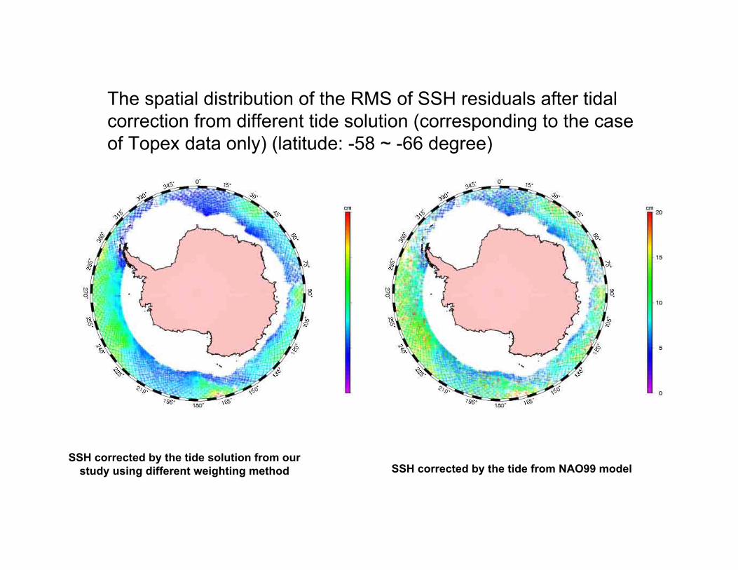
The spatial distribution of the RMS of SSH residuals after tidalcorrection from different tide solution (corresponding to the caseof Topex data only) (latitude: -58 ~ -66 degree)

SSH corrected by the tide solution from ourstudy using different weighting method SSH corrected by the tide from NAO99 model

SSH corrected by the tidefrom TPXO.6.2 model

SSH corrected by the tidefrom CATS02.01 model

As comparison, the same procedure is applied to use the altimetrydata at single satellite crossover locations to obtain the point-wisetidal solutions, and the following table shows their performance inreducing RMS of SSH compared with other models. (different weight)

16.18(4672)

15.27(10046)

15.18(10062)

11.62(10062)

22.40ERS-2

14.14(2020)

14.74(3068)

14.64(3070)

8.81(3070)

20.68Topex

CATS02.01TPXO.6.2NAO99Solutionof ourstudy

RMS of SSH residual after tidal correctionRMS ofSSH

beforetidal

correction

SSH Data atsingle satellite

crossoverpoints

intercomparison of tide solution using three weighting methods withNAO99 model and CATS02.01 model in terms of RSS (unit: cm)

12.9810.4713.5810.8914.5311.66ERS-2 data atsingle satellite

crossover points

1.981.721.981.721.981.72Topex data atsingle satellite

crossover points

2.342.162.412.222.382.22

Topex/ERS-2data at dual

satellite crossoverpoints

CATS02.01NAO99CATS02.01NAO99CATS02.01NAO99

Different weightConstant weight IIConstant weight I

intercomparison of tide solution using different weighting methodwith NAO99 model and CATS02.01 model in terms of vectorRMS for each tidal consitutent (unit: cm)

CATS02010.820.650.371.200.500.691.200.80

NAO.99b0.780.620.361.100.280.611.150.76ERS2_TPdata at dualsatellitecrossoverlocations

CATS02012.222.001.564.843.261.8910.712.18

NAO.99b1.871.721.183.592.661.598.711.89ERS2 data

at singlesatellite

crossoverlocations

CATS02010.700.500.311.060.450.531.030.65

NAO.99b0.620.460.300.890.190.460.950.58Topex data

at singlesatellite

crossoverlocations

ModelO1Q1P1K1K2N2S2M2DATA

Conclusion and future work

1. Based on the intercomparison results, the solutionusing Topex single satellite crossover data has thesmallest rms among the solutions using three kinds ofcrossover data.

2. Using TP_ERS2 dual satellite crossover data gives outbetter solution than using ERS-2 single satellitecrossover data, but a little worse solution than usingTopex single satellite crossover data only.

3. Our solutions using crossover data coincide with NAOand TPXO.6.2 model better than CATS0201 model,and the result show NAO model and TPXO.6.2 modelare comparable to each other as for the magnitude ofRMS.