sample synthesis, experimental techniques, and...
TRANSCRIPT
Chapter 2
Sample Synthesis, Experimental Techniques, and
Data-analysis Methodologies
This chapter deals with the description of sample preparation and various experi-
mental and computational techniques used to investigate the present thesis work.
The structural properties of the samples have been investigated by various tech-
niques such as X-ray and neutron diffraction, and differerential scanning calorimetry.
Bulk magnetic and magnetocaloric properties have been studied by dc magnetization
as a function of temperature and magnetic field. For microscopic understanding of
magnetic properties, temperature dependent neutron diffraction experiments have
been carried out. Mesoscopic technique neutron depolarization has been used to
study the magnetic properties of domains/clusters. For analyzing the X-ray and
neutron diffraction data, the Reidveld refinement method has been employed.
2.1 Sample synthesis
Polycrystalline samples of all intermetallic compounds investigated in this thesis
work were prepared by an arc-melting method. In this method, constituent elements
of high purity are taken in an appropriate stoichiometric ratio, and kept in a copper
crucible, which has a continuous supply of cold water to prevent melting of the
crucible. Some of the elements (e.g. Tb, Mn, Sb) were taken in excess amount to
compensate the evaporation losses. The furnace chamber is first maintained under
41

Chapter 2. Sample Synthesis, Experimental Techniques...... 42
a high vacuum of 10−3 torr and then flushed with an argon gas. This procedure is
repeated 2-3 times to ensure that no trapped gas molecules are present inside the
chamber. When the thoriated tungsten cathode is brought close to the anode(copper
crucible), an ionized argon gas in the chamber leads to an arc, which is used to
melt the elements under an argon atmosphere. The temperature of the arc can be
controlled by varying the current between two electrodes. In the set-up used for the
present thesis work, the current can be varied up to 270 A. The samples were re-
melted for four times to achieve a better chemical homogeneity. After melting, the
samples were annealed in vacuum-sealed quartz tubes at specific temperature for a
fixed duration. The annealing conditions vary for different intermetallic compounds.
The annealing of the samples was done to eliminate the possibility of any segregation
of other phases, by solid state diffusion.
2.2 Experimental techniques
2.2.1 X-ray diffraction
X-ray diffraction technique has been used to study the structural properties of the
intermetallic compounds. X-ray diffraction is based on the elastic scattering of X-
rays from the electron clouds of the individual atoms in the system, and yields the
atomic structure of materials. The diffraction pattern occurs due to the periodic
arrangements of atoms in space according to the Bragg’s Law
2dhklsinθhkl = nλ (2.1)
Here, θhkl is the Bragg angle, dhkl is the distance between two parallel atomic planes
for a given (hkl), λ is the wavelength of the X-ray, and n is an integer [36]. The
lattice parameters can be calculated from the position of the Bragg peaks [37]. A

Chapter 2. Sample Synthesis, Experimental Techniques...... 43
Bragg reflection can occur when λ ≤ 2d which means that the wavelength of the X-
ray should be of the order of the interatomic spacing. The X-rays are produced when
the high energy electron beam is bombarded on a metal target. For crystallography,
Cu is the most common metal target(which is also used in the present thesis work)
producing a wavelength i.e Cu (Kα) with λ = 1 .54187 A. The intensity of the
diffracted beam for a Bragg peak with Miller indices (hkl) is proportional to the
square of the structure factor F hkl, where
Fhkl =N∑
n=1
fn e2πi (hun+kvn+lwn) (2.2)
Here, f n is the atomic scattering factor for the nth atom in an unit cell, un, vn, wn
are the fractional atomic coordinates of an atom/ion within an unit cell, N is the
total number of atoms in an unit cell.
2.2.2 Neutron diffraction
Neutron diffraction experiments have been carried out at various temperatures, from
room temperature to down to 5 K, to study the structural and magnetic proper-
ties of the intermetallic compounds. The neutron diffraction patterns were recorded
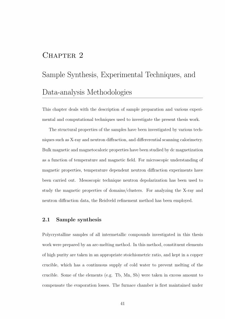
using the powder diffractrometer-II at the Dhruva reactor, Trombay, Mumbai, In-
dia (Figs. 2.1 and 2.2)[38]. The neutron wavelengths used were either λ = 1.249 or
1.2443 A. The scattering angular range of 5◦−130◦ is scaned by five one-dimentional
position sensitive dectetors with a resolution ( ∆d/d) of ∼ 1 %. The neutron flux
at the sample position is typically of the order of 8 × 10⁵ neutrons cm−2 s−1.
Temperature-dependent neutron diffraction patterns down to 1.5 K for one of the
samples (Cu0.85Ni0.15MnSb) were collected at the DMC cold neutron powder diffrac-
tometer (λ = 2.568 A), Paul Scherrer Institute, Switzerland. All other measurements
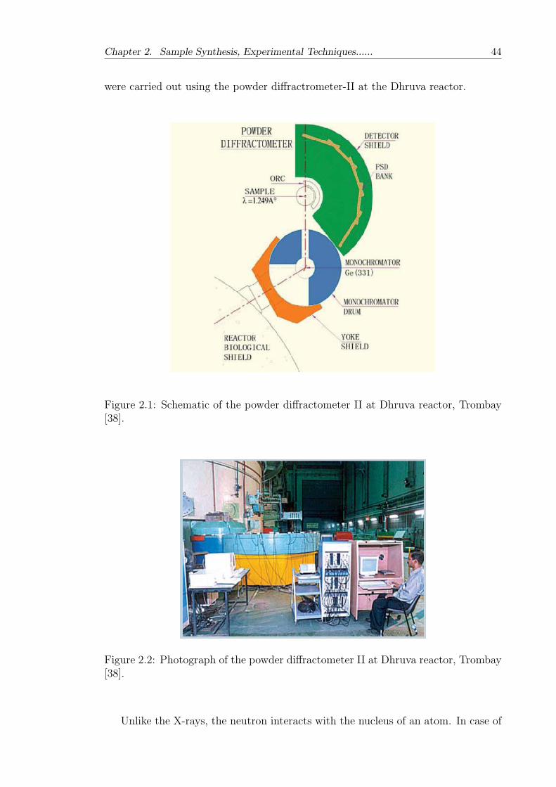
Chapter 2. Sample Synthesis, Experimental Techniques...... 44
were carried out using the powder diffractrometer-II at the Dhruva reactor.
Figure 2.1: Schematic of the powder diffractometer II at Dhruva reactor, Trombay[38].
Figure 2.2: Photograph of the powder diffractometer II at Dhruva reactor, Trombay[38].
Unlike the X-rays, the neutron interacts with the nucleus of an atom. In case of
Chapter 2. Sample Synthesis, Experimental Techniques...... 45
magnetic materials, the electronic scattering (due to magnetic interaction) is also
appreciable. The de Broglie wavelength of the thermal neutron is comparable to
the interatomic spacing (∼1 A) in solids, and hence thermal neutron diffraction is
suitable to study the crystal structure of solids. The physical properties of neutron
that make the neutron scattering complementary to X-ray scattering are:
(i) The neutron scattering is isotopic in nature as the nuclear dimension ( 10−15
m) is very small in comparison to wavelength of the thermal neutrons ( 10−10 m).
Therefore, in case of neutron-nuclear scattering, the scattering centers are point
particles. Hence, the neutron-nucleus scattering amplitude does not vary with the
scattering angle, whereas in the case of X-rays, the scattering is from the electron
clouds and the corresponding X-ray scattering amplitute shows a scattering vector
dependency.
(ii) The nuclear scattering cross-section for an atom is given by b2, where b is
nuclear scattering length. As b depends on the nuclear interaction, this scattering
length varies randomly across the periodic table and thus enables us to distinguish
between two nearby atoms of the periodic table. In the present thesis work where
we substitute one element by the nearby element of the periodic table, neutron
diffraction study helps us to confirm whether these atoms occupy the same site or
not. This is not possible in case of X-rays because the scattering cross-section for
X-rays depends on the atomic number (z), hence the variation of X-rays scattering
cross-section for two neighboring atoms in the periodic table is negligible.
(iii) Neutron possesses a magnetic moment of -1.913µN , where µN is the nuclear
magneton, and interacts with the magnetic moment of the atoms/ions. This helps to
determine the magnetic structure of the material by neutron scattering experiments.
In case of unpolarized neutrons, the Bragg diffracted intensity for a ferromagnetic
or a ferrimagnetic material is proportional to the square of the structure factors

Chapter 2. Sample Synthesis, Experimental Techniques...... 46
F 2hkl, [39] where
F 2hkl = F 2
nuclear + q2F 2magnetic
=
∣∣∣∣∣n∑
j=1
bj exp [2πi (hxj + kyj + lzj)] e−2Wj
∣∣∣∣∣2
+ q2
∣∣∣∣∣m∑j=1
pj exp [2πi (hxj + kyj + lzj)] e−2Wj
∣∣∣∣∣2
(2.3)
Here, bj is the scattering length of the j th nucleus which varies randomly across the
periodic table, n is the total number of atoms in a unit cell. The second term in Eq.
(2.3) gives the magnetic Bragg scattering which occurs if the magnetic moments
have a periodic arrangement. The magnetic interaction vector is given by
q = ϵ(ϵ ·K) −K, (2.4)
where K is a unit vector in the direction of the atomic magnetic moment and ε is
the scattering vector which is perpendicular to the effective ’reflecting’ planes.
pj =
(e2γ
2mc2
)Sjfj (2.5)
where S j is the magnetic moment of the j th atom, f j is the magnetic form factor of
the j th atom which rapidly decreases with (sin θ)/λ, γ is neutron magnetic moment
in nuclear magneton and e2/mc2 is the Bohr radius. x j, y j, z j are the fractional
atomic coordinates in an unit cell. For magnetic scattering, the summation is over
all (m) magnetic atoms/ions in the unit cell. e−2Wj is the Debye-Waller factor
for the j th atom, which is due to thermal fluctuations. For magnetic materials,
neutron diffraction carried out below the magnetic ordering temperature, gives the
information about the magnetic structure of the material, in addition to the crystal

Chapter 2. Sample Synthesis, Experimental Techniques...... 47
structure. In case of a ferromagnetic or ferrimagnetic material, additional Bragg
intensity to the lower angle fundamental nuclear peaks is observed. In case of
an antiferromagnetic material, where the magnetic unit cell could be larger than
the crystallographic unit cell, additional Bragg peaks appear corresponding to the
magnetic unit cell. To analyze the crystal structure as well as magnetic structure
using the neutron diffraction patterns, the Rietveld refinement technique [40] using
the FULLPROF program [41, 42] has been employed.
2.2.3 dc magnetization
The bulk magnetic properties of the intermetallic compounds under investigation in
this thesis have been investigated using (i) a vibrating sample magnetometer (VSM,
Oxford Instruments), (ii) a superconducting quantum interference device (MPMS
XL magnetometer, Quantum Design) also known as SQUID magnetometer, and
(iii) a Physical Property Measurement System (PPMS, Quantum Design). The
magnetization measurements have been carried out as a function of temperature
and applied magnetic field. The measurements have been carried in the temperature
range of 5-350 K and a magnetic field variation of up to ± 80 kOe.
2.2.3.1 dc magnetization using a vibrating sample magnetometer
The magnetic moment is measured by the induction technique in a VSM. This
technique was first given by S. Foner [43]. When a magnetic sample is placed in
a magnetic field produced by an electromagnet or by a superconducting magnet,
a dipole moment is induced. When the sample vibrates, an electromotive force
(electrical signal) is induced in the pick-up coil, which is given by
e = −NdϕB
dt(2.6)

Chapter 2. Sample Synthesis, Experimental Techniques...... 48
Here, e is the induced electromotive force, N is the number of turns in the coil, ϕB
is the magnetic flux in the coil and t is the time. If the sample moves along the
z-axis, then Eq. (2.6) can be written as
e = −NdϕB
dz
dz
dt(2.7)
If the sample vibrates with an amplitude a and frequency ω, then
z = a exp(iωt)
dz
dt= a i ω exp(iωt) (2.8)
Therefore
e = −N a i ωdϕB
dzexp(iωt) (2.9)
The induced emf of an unknown sample is compared with the induced emf of a stan-
dard sample such as nickel. When a standard nickel sample is used for calibration,
the induced emf of Ni (V Ni in volts) with known magnetic moment (MNi in emu)
is stored in calibration file. The magnetic moment of the unknown sample can then
be calculated as
Munknown = VunknownMNi
VNi
(2.10)
Powder samples are compressed in small spherical pellet form and loaded in the
sample holder located at the end of the sample rod. The other end of the sample rod
is connected to the vibrator of the VSM which vibrates vertically with an amplitude
fixed in the range of 0.1-1.5 mm and a fixed frequency of 43-67 Hz. For the present
thesis work, amplitude of 0.5 mm and frequency of 55 Hz have been used. The
ac signal at the pick-up coil is fed to a differential amplifier, and the output of
the amplifier is fed to a tuned amplifier and a lock-in amplifier which also receives a

Chapter 2. Sample Synthesis, Experimental Techniques...... 49
Figure 2.3: Photograph of the Vibrating Sample Magnetometer (Oxford Instru-ments) set up at Solid State Physics Division, BARC.
reference signal from the oscillator. The output of the lock-in amplifier is a dc signal
which is proportional to the magnetic moment of the sample under investigation.
All the data acquisition is done through computer.
2.2.3.2 dc magnetization using a SQUID magnetometer
SQUID (superconducting quantum interference device) is a very sensitive magne-
tometer. This is used to measure magnetic field or magnetization with the help of
superconducting loops with Josephson junction. The input current I splits into two
equal branches in the superconducting ring as shown in Fig. (2.3). If a magnetic field
B is applied perpendicular to the plane of the ring, a phase difference is produced
between currents in the two branches. The magnetic flux ϕ passing through the
superconducting ring is quantized in terms of h/2e, where h is the Plank’s constant
and 2e is the charge of the Cooper pair of electrons.

Chapter 2. Sample Synthesis, Experimental Techniques...... 50
Figure 2.4: Schematic diagram of a superconducting ring with Josephson junction ina superconducting quantum interference device (SQUID) as a simple magnetometer.
Some of the magnetization measurements were carried out using the SQUID
magnetometer (MPMS, Quantum Design). Measurement in MPMS is performed by
moving the sample through the superconducting detection coils which are located
at the center of the magnet. It measures the local changes in magnetic flux density
produced by a sample as it moves through the superconducting detection coils. The
sample moves along the symmetry axis of the detection coil and magnet. As the
sample moves through the coils, the magnetic dipole moment of the sample induces
an electric current in the detection coils. The SQUID functions as a highly linear
current-to-voltage convertor, so that variations in the current in the detection coil
circuit produce corresponding variations in the SQUID output voltage. The MPMS
determines the magnetic moment of a sample by measuring the output voltage of
the SQUID detection system as the sample moves through the coil.
2.2.3.3 dc magnetization using a physical property measurement system
dc magnetization measurement technique used in a Physical Property Measurement
System (PPMS) is the extraction magnetometry. In this technique, a magnetic

Chapter 2. Sample Synthesis, Experimental Techniques...... 51
sample is moved through the detection coils which in turn induces a voltage in
the detection coil set. The amplitude of the signal is proportional to the magnetic
moment as well as the speed of the sample during extraction. The dc servo mo-
tor used to move a sample can extract the sample at a speed of approximately
100 cm per second, thus significantly increasing the signal strength over conven-
tional extraction systems. The greater extraction speed also reduces any error that
may result from non-equilibrium time-dependent effects. The PPMS is provided
with AC/DC Magnetometry System (ACMS) which can perform ac susceptibility
Figure 2.5: Schematic of AC/DC Magnetometry System coil set [42].
Chapter 2. Sample Synthesis, Experimental Techniques...... 52
as well as dc magnetization measurements in a single sequence [44]. The ACMS
coil set includes the detection coils that measure the sample’s magnetic response.
The ACMS probe attachment is concentric with the primary dc superconducting
magnet. The detection coils are arranged in a first-order gradiometer configuration
which rejects background signals. The PPMS uses a Digital Signal Processor chip
rather than a lock-in amplifier which takes advantage of digital filtering. This sig-
nificantly improves signal-to-noise performance over analog filters, which have to
sacrifice accuracy in order to perform over a wide frequency band.
2.2.4 ac susceptibility
In ac susceptibility measurements, a small ac magnetic field is applied to the sample
which induces a time dependent magnetic moment in the sample. This induces time
dependent voltage in the pick-up coil. When the ac field is applied, the induced ac
moment of the sample is
Mac =dM
dHHac sin ωt (2.11)
where H ac is the amplitude of the ac field and ω is frequency, and dM /dH is the
slope of the M (H ) curve, called the susceptibility (χac). When the ac frequency is
low, the ac magnetization is similar to that of dc magnetization. But when the fre-
quency is high, the ac magnetization does not follow the dc magnetization curve due
to the dynamic of the sample. In this case, there is a lag between sample magnetiza-
tion and applied ac field. Thus the ac susceptibility is a complex quantity, and the
in and out of phase produce real and imaginary components of χac, usually denoted
as χ’ac and χ”ac, respectively. The frequency dependent ac susceptibility studies
help us to distinguish spin-glass, cluster spin-glass and superparamagnets. The out
of phase susceptibility component indicates a dissipative processes in the sample.
In case of ferromagnetic materials, this component indicates an irreversible domain
Chapter 2. Sample Synthesis, Experimental Techniques...... 53
wall movement. The relaxation and irreversibility of the magnetization also result in
out of phase susceptibility component. The technique complements dc susceptibility
technique by providing an additional frequency dependent information. Some of the
work in the present thesis has been carried out in a Physical Property Measurement
System with AC/DC Magnetometry System (ACMS) probe. The frequency range
is 10 Hz to 10 kHz and ac field is 5 Oe. The temperature range studied is 5 - 300 K.
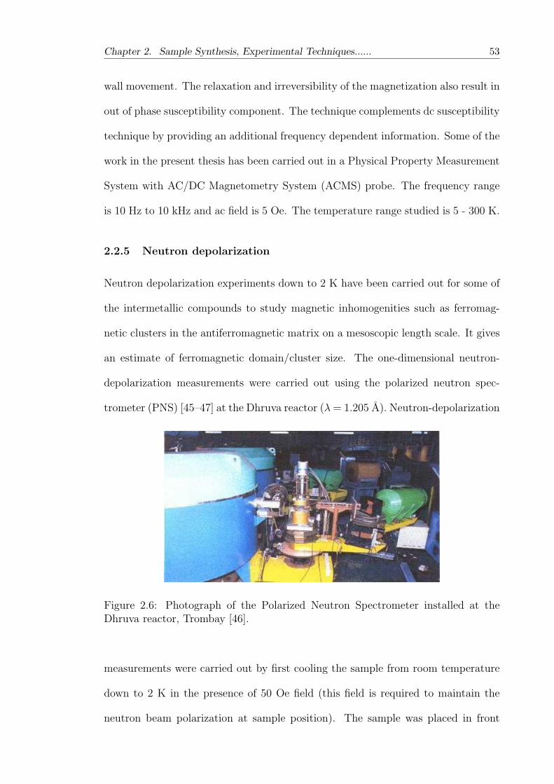
2.2.5 Neutron depolarization
Neutron depolarization experiments down to 2 K have been carried out for some of
the intermetallic compounds to study magnetic inhomogenities such as ferromag-
netic clusters in the antiferromagnetic matrix on a mesoscopic length scale. It gives
an estimate of ferromagnetic domain/cluster size. The one-dimensional neutron-
depolarization measurements were carried out using the polarized neutron spec-
trometer (PNS) [45–47] at the Dhruva reactor (λ = 1.205 A). Neutron-depolarization
Figure 2.6: Photograph of the Polarized Neutron Spectrometer installed at theDhruva reactor, Trombay [46].
measurements were carried out by first cooling the sample from room temperature
down to 2 K in the presence of 50 Oe field (this field is required to maintain the
neutron beam polarization at sample position). The sample was placed in front

Chapter 2. Sample Synthesis, Experimental Techniques...... 54
of the neutron beam such that the propagation direction of the polarized neutron
beam is along the thickness of the flat sample. The beam size was restricted within
the size of the sample. The incident neutron beam was polarized along the -z di-
rection (vertically down) with a beam polarization of 98.60(1) %. In case of an
unsaturated ferromagnet or ferrimagnet, the dipolar field exerted by the magnetic
domains on the neutron polarization depolarizes the neutrons due to Larmor pre-
cession of the neutron spins in the magnetic field of domains. In a ferromagnetic
domain, the spin component parallel to the magnetic induction B does not precess
whereas the component perpendicular to B does. The precession angle is given as
Φδ = (4.63×10⁻¹⁰ G−1 A−2)λδB where λ is the wavelength of the neutrons and
δ is the effective thickness i.e. distance traveled by the neutrons. The value of
average magnetic induction B = 4πM S (in Gauss) was estimated from the bulk
magnetization measurements where M S is the spontaneous magnetization and ρ is
the density of the material in g cm−3. In a pure antiferromagnet, there is no net
magnetization, hence no depolarization occurs. In case of a true spin-glass state,
the spins are randomly frozen in space on a microscopic length scale and hence no
net magnetization is present, resulting in no depolarization. In a paramagnet, the
neutron polarization is unable to follow the variation in the magnetic field as the
temporal spin fluctuation is too fast (10−12 s or faster). Hence, no depolarization is
observed. However, depolarization is expected in case of clusters of spin with a net
magnetization [48]. The neutron beam polarization in a depolarization experiment
can be represented by the following expression
Pf = Pi exp
[−α
(d
δ
)⟨Φδ⟩2
](2.12)

Chapter 2. Sample Synthesis, Experimental Techniques...... 55
where P i and P f are the initial and final neutron beam polarizations, α is a di-
mensionless parameter ≈ 1/3, d is effective sample thickness, and δ is the average
domain size. Equation (2.12) is valid only when the precession angle Φδ is a small
fraction of 2π over a typical domain/cluster length.
In a neutron delpolarization study we measure the polarization ratio (R) which
is a measure of the transmitted polarization. The expression for the polarization
ratio is given by
R =1 − PiDPA
1 + (2f − 1)PiDPA
(2.13)
where PA is the efficiency of the analyzer, f is the efficiency of the rf flipper and D
is the depolarization coefficient. P iD is the transmitted beam polarization. When
there is no depolarization, D = 1 and, when there is total depolarization, D = 0.
2.2.6 Differential scanning calorimetry
Differential scanning calorimetry (DSC) measurements were carried out on some of
the intermetallic compounds using the Mettler Toledo DSC 822 set up which is of
heat flux type. This technique can be employed to investigate a system undergoing
structural phase transition. In differential scanning calorimetry, the difference in
the amount of heat required to increase the temperature of a sample with respect to
the reference is measured as a function of temperature. This technique is based on
the fact that when a sample undergoes a physical transformation such as a phase
transition, either heat is required or librated out of the sample with respect to that
of the reference to maintain both at the same temperature. Whether heat flows out
of the sample or into the sample depends on whether the process is exothermic or
endothermic. In the present work, an empty aluminum pan was used as a refer-
ence. The sample was encapsulated in another aluminum pan and then carefully
placed in the DSC cell. The measurements were carried out in the heating as well as

Chapter 2. Sample Synthesis, Experimental Techniques...... 56
cooling cycles with a scanning rate of 5 K/min. The heat flow versus temperature
was recorded as output. Near the phase transition temperature of a sample, the
absorption or evolution of heat causes a change in the differential heat flow, which
appears as a peak. The peak position of the DSC curve gives the transition temper-
ature of the sample. This curve can be used to calculate enthalpies of transitions.
The integrated area under the peak gives the enthalpy change accompanying the
transition. The nature of the curve also gives the information about the order of
the phase transition. Specific heat capacities and changes in heat capacity can also
be determined from the difference in heat flow.
2.3 Computational techniques
2.3.1 Rietveld refinement
Rietveld refinement technique [40, 49, 50] has been employed to analyze the X-ray
and neutron diffraction patterns. FULLPROF program [41, 42] has been employed
to refine the crystal structure by using the X-ray diffraction patterns. This program
was also employed to refine the crystal structure and to determine the magnetic
structure from neutron diffraction patterns. Rietveld refinement is based on least-
squares minimization technique. This technique minimizes the difference between
experimental powder diffraction pattern and a calculated pattern based on a model
crystal structure and instrumental parameters. This technique can be used to de-
rive certain parameters such as lattice parameters, atomic positions and their oc-
cupancies, thermal parameters, magnetic moment and its direction, phase fraction,
etc. The Rietveld refinement method consists of refining a crystal and/or magnetic
structure by minimizing the weighted squared difference between observed intensity
{y i}i=1...n and calculated intensity { yc,i(α) } i=1...n against a set of parameters (α)
Chapter 2. Sample Synthesis, Experimental Techniques...... 57
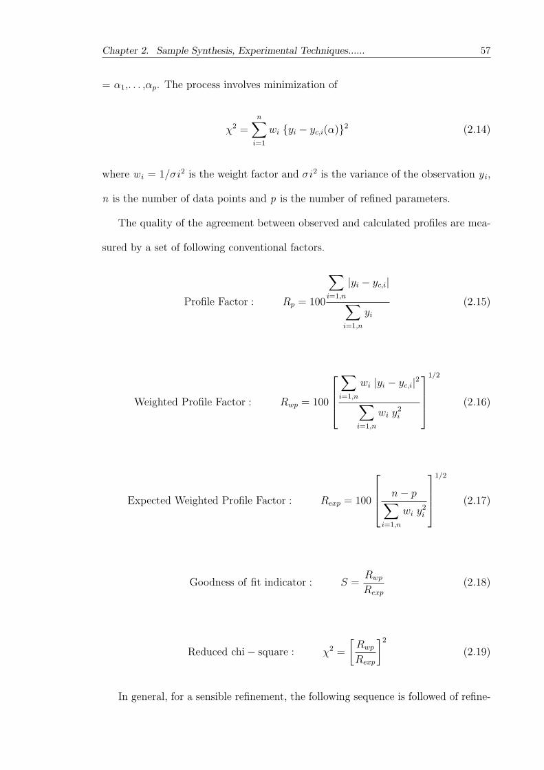
= α1,. . . ,αp. The process involves minimization of
χ2 =n∑
i=1
wi {yi − yc,i(α)}2 (2.14)
where w i = 1/σi2 is the weight factor and σi2 is the variance of the observation y i,
n is the number of data points and p is the number of refined parameters.
The quality of the agreement between observed and calculated profiles are mea-
sured by a set of following conventional factors.
Profile Factor : Rp = 100
∑i=1,n
|yi − yc,i|∑i=1,n
yi(2.15)
Weighted Profile Factor : Rwp = 100
∑i=1,n
wi |yi − yc,i|2∑i=1,n
wi y2i
1/2
(2.16)
Expected Weighted Profile Factor : Rexp = 100
n− p∑i=1,n
wi y2i
1/2
(2.17)
Goodness of fit indicator : S =Rwp
Rexp
(2.18)
Reduced chi − square : χ2 =
[Rwp
Rexp
]2(2.19)
In general, for a sensible refinement, the following sequence is followed of refine-
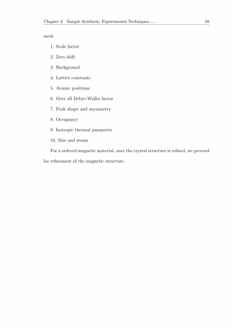
Chapter 2. Sample Synthesis, Experimental Techniques...... 58
ment
1. Scale factor
2. Zero shift
3. Background
4. Lattice constants
5. Atomic positions
6. Over all Debye-Waller factor
7. Peak shape and asymmetry
8. Occupancy
9. Isotropic thermal parameter
10. Size and strain
For a ordered magnetic material, once the crystal structure is refined, we proceed
for refinement of the magnetic structure.