Popular summary for:

High-frequency planetary waves in the polar middle atmosphere as seen in a

data assimilation system

L. Coy, I. Stajner, A.M. da Silva, J. Joiner, R.B. Rood, S. Pawson, S.J. Lin

for submission to The Journal of the Atmospheric Sciences

The atmosphere displays a wide range of motions with different and spatial

and temporal structures. Many of these disturbances can be described as

Rossby waves with specific wavenumber and frequency. One example is

the quasi-two-day wave, which has been detected in ground-andspace-based

observations of temperature and winds in the upper stratosphere and lower

mesosphere. This study presents the first evidence of such a wave in the

assimilated datasets produced by NASA's Data Assimilation Office. The

study examines assimilated meteorology and ozone in July 1998, showing a

significant signal in all of these quantities, representing a major source of

ozone variation in the stratopause region. It is shown that the wave in the

ozone assimilation is in good agreement with that inferred from data of the

"Polar Ozone and Aerosol Measurement (POAM)" satellite. The two-day

wave in the polar region is shown to arise in conjunction with linear

instabilities of the flow, since it is associated with Eliassen-Palm flux

divergence in regions of negative gradients of potential vorticity.

https://ntrs.nasa.gov/search.jsp?R=20030025379 2018-07-29T17:51:45+00:00Z

High Frequency Planetary Waves in the Polar

Middle Atmosphere as seen in a Data

Assimilation System

L. coy *

E. 0. Hulburt Center for Space Research, Naval Research Laboratory

Washington, DC

I. Stajner A. M. DaSilva J. Joiner R. B. Rood

S. Pawson

S. J. Lin

NASA Goddard Space Flight Center, Greenbelt, Maryland, USA.

*Corresponding author address: Lawrence Coy E. 0. Hulburt Center for Space Research, Naval Research Laboratory, Code 7646 4555 Overlook Avenue SW, Washington, JX 20375-5320, USA. Tel: (202) 404-1266 , Fax: (202) 404-8090, e-mail: coy@uap2.nrl.navy.mil

ABSTRACT

This study examines the winter southern hemisphere vortex of 1998 using four

times daily output from a data assimilation system to focus on the polar 2-day, wave

number 2 component of the 4-day wave. The data assimilation system products are

from a test version of the finite volume data assimilation system (fvDAS) being de-

veloped at Goddard Space Flight Center (GSFC) and include an ozone assimilation

system. Results show that the polar 2-day wave dominates during July 1998 at 70"s.

The period of the quasi 2-day wave is somewhat shorter than 2 days (about 1.7 days)

during July 1998 with an average perturbation temperature amplitude for the month of

over 2.5 K. The 2-day wave propagates more slowly that the zonal mean zonal wind,

consistent with Rossby wave theory, and has EP flux divergence regions associated

with regions of negative horizontal potential vorticity gradients, as expected from lin-

ear instability theory. Results for the assimilation-produced ozone mixing ratio show

that the 2-day wave represents a major source of ozone variation in this region. The

ozone wave in the assimilation system is in good agreement with the wave seen in the

POAM (Polar Ozone and Aerosol Measurement) ozone observations for the same time

period. Some differences with linear instability theory are noted as well as spectral

1

peaks in the ozone field, not seen in the temperature field, that may be a consequence

of advection.

2

1 Introduction

The 4-day wave is a relatively common planetary-scale stratopause disturbance found

mainly during the southern hemisphere winter. This high latitude wave consists of

wave 1 and 2 (and some higher wavenumber) components moving at nearly the same

rotational period (the time for a crest to travel around a latitude circle), about 3 4 days,

so that the period of the wave 2 component is about 1.5-2 days. Many studies of

the 4-day wave have focused on the wave 1 component as only daily analyses are

needed to resolve the period accurately. However, modem data assimilation systems

that include the stratosphere often output 4 times a day and so can be used to examine

the higher frequency wave 2 component of the 4-day wave. This paper presents results

of the 4-day wave seen in the temperature and ozone fields produced by a global data

assimilation system during a time when the wave 2 component was dominant.

The 4-day wave has been described by Venne and Stanford (1979, 1982), Prata

(1984), Lait and Stanford (1988), Randel and Lait (1991), Manney (1991), Lawrence

et al. (1995), and Lawrence and Randel (1996): more references can be found in Allen

et al. (1997). Most of these studies examined satellite radiances, though Manney (1991)

used daily analyses from the NCEP (National Center for Environmental Prediction)

data assimilation system. The wave originates near the stratopause at the level of the

3

stratospheric jet maximum where the latitudinal mean zonal wind shears tend to be

largest. The wave is believed to be generated by barotropic and baroclinic instability,

the relative importance of either process depending on the particular zonal mean wind

configuration.

The linear barotropic instability problem at the stratopause germane to 4-day wave

genesis was first investigated by Hartmann (1983) for idealized latitudinal zonal wind

profiles. Hartmann (1983) found that instabilities could occur on both the poleward

and equatorward side of jets corresponding to negative zonal mean potential vorticity

gradients on both sides of the jet. The zonal phase speeds of the unstable waves were

nearly equal to the mean zonal wind speed where Qy (the zonal mean potential vorticity

gradient) changed sign. This gives shorter rotational periods on the poleward side of

the jet (-4 days) and longer rotational periods on the equatorward side of the jet (-15

days) because of the change in length of latitude circles around the globe, even though

the phase speeds could be similar on both sides of the jet. Using a quasi-geostrophic

model Hartmann (1983) also found that baroclinic effects tended to stabilize and re-

duce growth rates by confining the vertical extent of the region of strong latitudinal

wind shear. In Hartmann (1983) both wavenumbers 1 and 2 had similar growth rates,

however, another barotropic model study (Manney et al. 1988) showed L!at wave 2

became the more unstable mode (rather than wave 1) as the jet became more sharply

4

peaked. Manney et al. (1988) also showed that the waves became more dispersive

(that is, the rotational period had more variation for different wave numbers) as the jet

moved equatorward.

Manney and Randel (1993) used a linear quasigeostrophic model to examine un-

stable modes in climatological zonal mean winds, including both barotropic and baro-

clinic effects. They showed that both effects were necessary for realistic growth rates

to occur in the zonal mean winds they studied, These results agreed with observational

studies (Randel and Lait 1991) that showed strong vertical Eliassen-Palm (EP) fluxes

in some 4-day wave observations. More recent work by Allen et al. (1997) highlighted

the general structure of the 4-day wave in terms of the temperatures, winds, and heights

associated with a potential vorticity (pv) anomaly.

Stratospheric constituents can respond to the 4-day wave as tracers if they have

mean gradients in the wave region and relatively long chemical lifetimes. Using high-

latitude middle atmosphere observations from UARS (Upper Atmosphere Research

Satellite) Allen et al. ( I 997) showed a 4-day signal in ozone while Manney et al. (1998)

showed a 4-day signal in water vapor and methane. Both studies modeled the tracers

differently. Allen et al. (1997) calculated the linear ozone response to the observed

temperatlire and geostrophic meridional wind signal coupled with simple phoiochem-

istry to examine the vertical structure of the ozone signal. Manney et al. (1998) used

5

an isentropic transport model to examine how tracers were transported from low lati-

tudes into the wave region. Both studies showed that the 4-day wave, when active, can

explain a large amount of the tracer variability near the polar stratopause.

This paper reports on the higher frequency, wave 2 component of the 4-day wave

using 6 hourly output from a data assimilation system that includes output from an off-

line ozone assimilation as well as the standard assimilation-produced mass and wind

fields. Following a brief description of the assimilation products and analysis methods

(section 2) the assimilation based 4 day wave diagnostics are presented (section 3). In

addition to the ozone assimilation the 4 day wave can be seen in POAM observations

(section 4).

2 Analysis

This study uses assimilation products from the Data Assimilation Office (DAO) at

NASA's Goddard Space Flight Center (GSFC). Output is taken from a developmen-

tal system (fvDAS: finite volume Data Assimilation System) that was run for the year

1998. This system is based on the new fvGCM (finite volume General Circulation

Model) coupled with the PSAS (Physical space Statistical Analysis System) analysis

system (Cohn et al. 1998) that are used together in the current DAO operation sys-

6

tem. As in the current DAO production system, the top analysis level is 0.4 hPa with

the actually model top at 0.01 hPa, making this a good system for stratopause studies.

Output from the fvDAS includes zonal and meridional winds, temperature, and geopo-

tential heights on 36 pressure levels from 1000-0.2 hPa at a horizontal resolution of

2.5" longitude by 2" latitude. These output fields were saved every 6 hours.

Satellite radiances are the main data going into the assimilation system in the up-

per stratosphere levels of interest here. Until July 1998, data from the NOAA 11 and

NOAA 14 TOVS (TIROS Operational Vertical Sounder) were assimilated. TOVS con-

sists of the High-resolution Infrared Sounder (HIRS), a 20 channel IR filter-wheel

radiometer, SSU (Stratospheric Sounding Unit), a 3 channel radiometer that uses a

pressure-modulation technique, and MSU (Microwave Sounding Unit), a 4 channel

microwave radiometer. The channels affecting the upper stratosphere are the 2 high-

est peaking SSU channels and HIRS channel 1. To avoid inter-satellite biases (upper

stratospheric channels are not bias-corrected), the NOAA 11 SSU channels were not

assimilated. After 1 July 1998, data from the NOAA 15 Advanced TOVS (ATOVS)

were added to the assimilation, where the 15 channel Advanced Microwave Sounding

Unit (AMSU) replaced the SSU and MSU of previous NOAA satellites. To avoid inter-

satellite bias between the N O M 15 ATDVS and tbe MOAA 14 SSU, the N0.4A-14

SSU channels were not assimilated after 1 July 1998. The radiances were assimilated

7

using a IDVAR algorthm (Joiner and Rokke 2000).

In addition to the regular assimilation system, an off-line ozone assimilation has

been run for the same time period (1998) using the fvDAS winds and temperatures as

input (Stajner et al. 2001). The assimilation uses satellite-based ozone observations

from SBUV (Solar Backscatter Ultra-Violet) for profile information and from TOMS

(Total Ozone Mapping Spectrometer) for a total column constraint. The ozone fields

are available on the same grid and at the same times as the fvDAS assimilation de-

scribed above.

A standard Fourier transform package was used on two dimensional longitude by

time arrays to extract the eastward propagating wave components of interest at a given

latitude and height. The Fourier analysis was performed monthly (120-124 points in

time). The westward propagating modes consist mainly of solar tidal periods and are

not shown here. Though some higher wavenumber components also show the 4-day

wave, only the dominant wave 1 and wave 2 components are presented here. EP fluxes

and associated heat and momentum fluxes were calculated for a given wavenumber and

frequency from the zonal wind, meridional wind, and temperature Fourier coefficients

along with the zonal and monthly averaged zonal winds and temperatures. The EP flux

formulas were evaluated using spherical, log-pressure coordinates (see Andrews et al.

1987, equations 3.5.3a and b, page 128).

8

3 Results

The 4-day wave is easily seen in the gridded assimilation products. Fig. 1 shows lon-

gitude time sections for temperature and ozone mixing ratio at 70"s and 2 hPa for

July 1998. Both fields show wave 2 features propagating eastward with periods of

about 2 days. The peak-to-peak amplitude is on the order of 10 K for temperature and

1 ppmv for ozone. A comparison with independent POAM ozone observations will be

given later.

Fig. 2 gives a mid-July, 2 hPa synoptic view of the South Pole where the wave 2

structure can be easily seen. The temperature field (Fig. 2a) shows two warm regions

with a cold, elongated region in between, located over the pole. Both of these warm

regions are also seen in the UKMO (United Kingdom Meteorological Office) strato-

spheric assimilation (not shown) so the warm regions are unlikely to be a DAO system

artifact. However, there are differences in temperatures between the two analyses that

reflect the difficulties still associated with temperature analyses near the stratopause.

The Ertel potential vorticity (pv) field (Fig. 2b) shows a strong gradient associated with

the main polar vortex and a weaker, inner vortex, associated with the wave 2 feature.

Ozone (Fig. 2c) also shows an elongated wave 2 low ozone region near the pole. The

phase of the ozone wave disturbance is somewhat east of the temperature and pv waves.

9

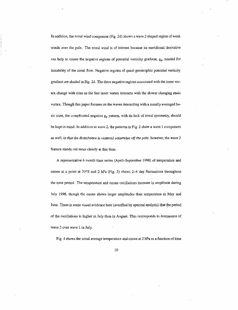
In addition, the zonal wind component (Fig. 2d) shows a wave 2 shaped region of weak

winds over the pole. The zonal wind is of interest because its meridional derivative

can help to create the negative regions of potential vorticity gradient, qy, needed for

instability of the zonal flow. Negative regions of quasi-geostrophic potential vorticity

gradient are shaded in Fig. 2d. The three negative regions associated with the inner vor-

tex change with time as the fast inner vortex interacts with the slower changing main

vortex. Though this paper focuses on the waves interacting with a zonally averaged ba-

sic state, the complicated negative qy pattern, with its lack of zonal symmetry, should

be kept in mind. In addition to wave 2, the patterns in Fig. 2 show a wave 1 component

as well, in that the disturbance is centered somewhat off the pole: however, the wave 2

feature stands out more clearly at this time.

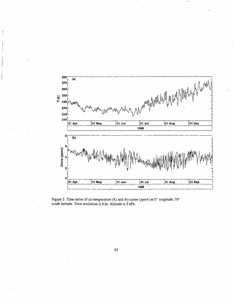
A representative 6 month time series (April-September 1998) of temperature and

ozone at a point at 70"s and 2 hPa (Fig. 3) shows 2-4 day fluctuations throughout

the time period. The temperature and ozone oscillations increase in amplitude during

July 1998, though the ozone shows larger amplitudes than temperature in May and

June. There is some visual evidence here (averified by spectral analysis) that the period

of the oscillations is higher in July than in August. This corresponds to dominance of

wave 2 over wave 1 in July.

Fig. 4 shows the zonal average temperature and ozone at 2 hPa as a function of time

10

and latitude. While the ozone gradients increase somewhat with time, the temperature

structure changes dramatically in July 1998, with a relatively warm region forming at

60-70"s and increased meridional temperature gradients poleward of 70"s. As will be

shown, this warm region is where the wave 2 component of the 4-day wave is found.

Fig. 5 shows the July 1998 eastward propagating temperature and ozone frequency

spectrum as a function of pressure at 70"s for wave 1 and wave 2. Also plotted is

the critical line, derived from the zonal mean zonal wind, for each frequency and

wavenumber. Note that most wave activity is bounded by the critical line indicating

that the waves are regressing with respect to the zonal mean winds as expected for

Rossby waves. The wave 1 temperature spectra (Fig. 5a) are large for the station-

ary and slowly propagating waves, however the amplitudes are relatively weak and

poorly defined near the 4-day wave frequency (0.25 day-l). The wave 1 ozone spec-

tra (Fig. 5b) show a stationary wave peak at 2 hPa and a weak ozone peak at a fairly

high period (0.4 day-l) very near the critical level. The wave 2 temperature spectra

(Fig. 5c) show a large, vertically coherent peak at about 0.6 day-l. This is the wave 2

structure: the period is about 1.7 days. The spectral peak maximizes between 1-2 hPa

and extends from the top of the domain down to the critical level. The wave 2 ozone

specua (Fig. 56) shows a simiiar 0.6 day-l peak, thoilgh it is milch mme localized in

the vertical than the wave 2 temperature peak. Ozone also tends to show a weak peak

11

at higher frequencies near the critical level, similar to the wave 1 ozone spectra.

The same frequencies as a function of latitude, at 2 hPa, are shown in Fig. 6. Once

again the waves are generally constrained by the critical line to be propagating more

slowly than the zonal mean flow. An exception seen here is near the equator where the

peaks in the temperature spectra are likely to be Kelvin waves. The wave 1 tempera-

ture spectra (Fig. 6a) show the largest amplitudes at low frequencies (periods greater

than 10 days). Poleward of 70"s there is a weak peak at 0.25 day-'. The wave 1

ozone spectra (Fig. 6b) show low frequency waves along with high frequency peaks

poleward of 70"s. As in Fig. 5, the ozone tends to show peaks near the critical level

and peaks at even higher frequencies than the critical level frequency. The wave 2

temperature spectra (Fig. 6c) show low frequency waves equatorward of 60"s and the

high frequency peak, as before, at 0.6 day-l. The wave 2 ozone spectra (Fig. 6d) also

show the 0.6 day-' peak, along with peaks at higher frequencies near the critical level.

The tendency seen here for the ozone frequencies to peak near the critical level may

represent advection of ozone features by the zonal mean wind and is discussed further

in Section 5. Fig. 6 shows that the high frequency wave is larger and more well defined

in wave 2 than wave 1 during July 1998 in agreement with Fig. 5 .

As pointed out by Allen et al. (1997) and others, tine 4-day wave temperature struc-

ture is expected to be a vertical dipole centered about a geopotential height (or pv)

12

perturbation. The two lobes of the temperature dipole will be out of phase with each

other so that high perturbation heights will have warm air below and cold air above,

consistent with hydrostatic balance. In this study, only the lower lobe of the tempera-

ture dipole can been seen, as the DAO pressure level output stops at 0.2 hPa. However,

the geopotential height and pv waves can be examined above the lower temperature

lobe.

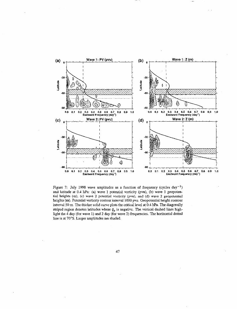
Figure 7 shows the wave 1 and wave 2 pv and geopotential height spectra for

July 1998 at 0.4 hPa as a function of latitude. The pv and height spectra are simi-

lar. The wave 1 spectra (Figs. 7a and b) show the largest peaks for the low frequency

waves with smaller peaks poleward of W S at 0.25 day-' and higher frequencies. The

wave 2 spectra (Figs. 7c and d) show some low frequency waves equatorward of 60's

and a well-defined high frequency peak at 0.6 day -l. This wave 2 peak occurs near the

intersection of the critical line and the latitude where gy = 0. This agrees with expecta-

tions from the linear theory of barotropically growing waves (as discussed in Hartmann

1983). Because of the double-peaked jet at these altitudes, the wave 2 frequencies from

0.55-0.6 day-l actually have three critical lines (as can be seen in Fig. 7), and the two

most poleward critical lines are close to the two qv = 0 lines that bound the negative

sl, region between the two jets. Thus, the monthiy averaged zonal mean zonal wind in

July 1998 provides ample opportunity for the development of wave 2 , 0 3 4 . 6 day-l

13

modes. What is not clear is why wave 2 is singled out for development rather than the

corresponding wave 1 frequencies.

The next three plots (Figs. 8,9, and 10) present a series of latitude-pressure sections

of the July 1998 wave 2 structure at a single frequency, 0.58 day-' (1.72 day period),

that corresponds to the main wave 2 peak seen in the spectra. The critical line for this

frequency is repeated on all the plots as a reference curve. Note that these plots are

more limited in altitude (100-0.2 hPa) and latitude (90-30's) than previous plots to

better focus on the region of interest.

Figure 8a shows the zonal mean zonal wind for the month of July 1998 and its

associated negative region of gu. The jet tilts strongly equatorward with altitude with a

weak poleward secondary maximum at the uppermost levels. In between the two jets

is the negative gv region. The critical line for the 0.58 day-l wave and the Q = 0

line coincide at upper levels, in the region between the two jets. The reference level

at 0.4 hPa shows how there can be three critical levels at a given altitude as seen in

Fig. 7. Figure 8b shows the zonal mean temperatures for July 1998. The dashed line

shows where the meridional temperature gradient is zero. A region of reversed temper-

ature gradient (warm air toward the pole) extends from the mesosphere down into the

stratosphere.

Figure 8c shows the wave 2 temperature amplitude and phase. As mentioned above,

14

only the lower lobe of the temperature structure is seen at these altitudes, though the

phase is changing rapidly with height at the top level, as expected, and there is some

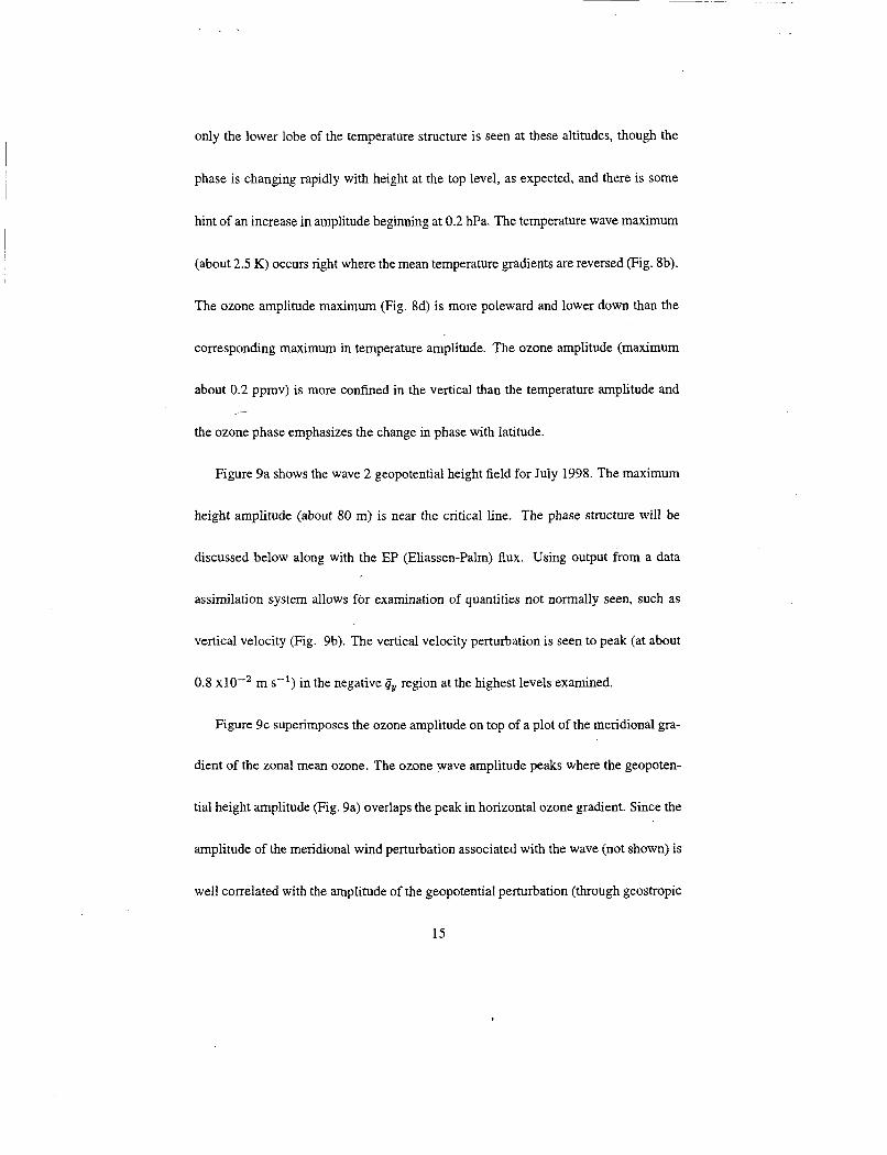
hint of an increase in amplitude beginning at 0.2 hPa. The temperature wave maximum

(about 2.5 K) occurs right where the mean temperature gradients are reversed (Fig. 8b).

The ozone amplitude maximum (Fig. 8d) is more poleward and lower down than the

corresponding maximum in temperature amplitude. The ozone amplitude (maximum

about 0.2 ppmv) is more confined in the vertical than the temperature amplitude and /

the ozone phase emphasizes the change in phase with latitude.

Figure 9a shows the wave 2 geopotential height field for July 1998. The maximum

height amplitude (about 80 m) is near the critical line. The phase structure will be

discussed below along with the EP (Eliassen-Palm) flux. Using output from a data

assimilation system allows for examination of quantities not normally seen, such as

vertical velocity (Fig. 9b). The vertical velocity perturbation is seen to peak (at about

0.8 x ~ O - ~ m s-l) in the negative &, region at the highest levels examined.

Figure 9c superimposes the ozone amplitude on top of a plot of the meridional gra-

dient of the zonal mean ozone. The ozone wave amplitude peaks where the geopoten-

tial height amplitude (Fig. 9a) overlaps the peak in horizontal ozone gradient. Since the

amplitude of the meridional wind perturbation associated with the wave (not shown) is

well correlated with the amplitude of the geopotential perturbation (through geostropic

15

balance) this implies that horizontal advection by the wave acting in a region of strong

latitudinal ozone gradients is mainly responsible for the ozone wave signal, in agree-

ment with the findings of Manney et al. (1998).

Figure 9d shows that temperature is not the only quantity with a dipole structure.

The zonal mean wind perturbation shows a strong dipole structure in latitude associated

with the height perturbation. A phase switch occurs between the two lobes. This

structure is expected from geostrophic balance with the perturbation height field. The \

most equatorward lobe peaks at -50's.

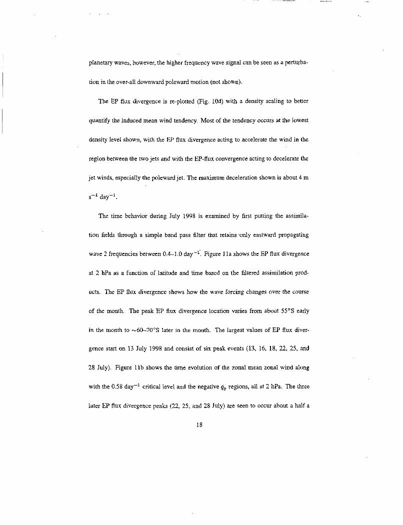
Figure 10a plots the EP flux divergence and the EP flux vectors calculated from the

assimilated winds and temperatures for July 1998 wave 2 height field. The divergence

is centered at about 1 hPa and 58"s with extensions up into the negative oy region and

across over a broad latitude range (70-5OOS) at 2 hPa. The EP flux vectors point into

three convergence regions: equatorward (and above), poleward (and above) and below

the divergence region. Linear instability theory predicts growing waves to consist of a

dipole of EP flux divergence and convergence with the EP flux vector pointing from di-

vergence to convergence (see Hartmann (1983) for a discussion of the barotropic prob-

lem and Manney and Randel (1993) for baroclinic examples). The July 1998 wave 2

shows a more complex case than what 1s usually modeled. T i e poleward and equator-

ward EP flux vectors show that both poleward and equatorward momentum fluxes are

16

associated with the wave. This helps explain the geopotential height field phase vari-

ations shown in Fig. 9a at upper levels where the meridional phase gradient changes

sign. Downward EP flux vectors have been reported by Randel and Lait (1991) and

Allen et al. (1997) and in the linear instability model of Manney and Randel (1993).

These downward EP flux vectors are not surprising in a middle atmosphere instabil-

ity event: however, they contrast with the usually upward direction associated with

planetary waves propagating upward from the troposphere. The net EP flux will still

be upward, of course, as the forced upward planetary fluxes are much larger than the

fluxes associated with the local instability. These downward EP flux vectors penetrate

to below 10 hPa where they abate near the lower part of the critical level.

Figure 10b shows the same fields as in Fig. loa, but calculated using only the assim-

ilated geopotential height field amplitude and phase shown in Fig. 9a, using the quasi-

geostrophic approximation. Though the magnitudes are larger, the quasi-geostrophic

approximation shows remarkable agreement with the full calculation. This lends sup-

port to observational EP-flux studies based only on satellite derived height fields.

Figure 1Oc plots the heat flux-based mass stream function (meridional heat flux di-

vided by the mean stability) associated with the 0.58 day-' wave 2. The circulation is

equatorward at 2 hPa, opposite to the poleward motion forced by upward propagating

planetary waves. The total circulation will be dominated by the upward propagating

17

planetary waves, however, the higher frequency wave signal can be seen as a perturba-

tion in the over-all downward poleward motion (not shown).

The EP flux divergence is re-plotted (Fig. 10d) with a density scaling to better

quantify the induced mean wind tendency. Most of the tendency occurs at the lowest

density level shown, with the EP flux divergence acting to accelerate the wind in the

region between the two jets and with the EP-flux convergence acting to decelerate the

jet winds, especially the poleward jet. The maximum deceleration shown is about 4 m

s-' day-'.

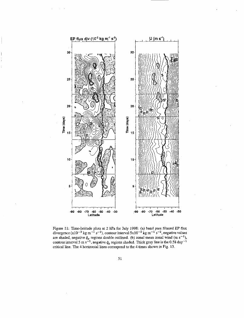
The time behavior during July 1998 is examined by first putting the assimila-

tion fields through a simple band pass filter that retains.only eastward propagating

wave 2 frequencies between 0.4-1 .O day-l'. Figure 1 l a shows the EP flux divergence

at 2 hPa as a function of latitude and time based on the filtered assimilation prod-

ucts. The EP flux divergence shows how the wave forcing changes over the course

of the month. The peak EP flux divergence location vanes from about 55"s early

in the month to -60-70"s later in the month. The largest values of EP flux diver-

gence start on 13 July 1998 and consist of six peak events (13, 16, 18, 22, 25, and

28 July). Figure l l b shows the time evolution of the zonal mean zonal wind along

with the 0.58 day-' critical level and the negative qv regions, aii at 2 hPa. The three

later EP flux divergence peaks (22, 25, and 28 July) are seen to occur about a half a

18

day after the center of corresponding negative qy regions. There is also some overlap

between the EP flux divergence on 9 July and a negative gy region.

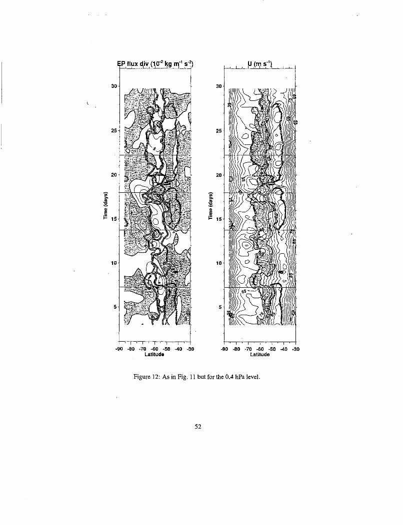
Figure 12 shows the same fields as Fig. 11 at 0.4 hPa. The zonal mean zonal wind

(Fig. 12b) shows the double jet structure at these altitudes with a persistent region of

negative I& located between the two jets. Unlike the nearly constant single critical line

at 2 hPa, at 0.4 hPa there are often times when the 0.58 day-' critical line is found at

three latitudes. Note how the 0.58 day-' critical line mirrors the poleward most i&, = 0

line during most of the time shown and tracks closely the middle critical line about half

of the time shown. The EP flux divergence at 0.4 hPa is mainly in the negative qy

region with EP flux convergence outside the negative i&, region as expected from linear

stability arguments for growing waves. This relation is especially apparent on 14 July.

Figure 13 shows the EP flux divergence and the zonal mean zonal wind at 4 times:

7 Jul 6 UTC; 13 Jul 18 UTC; 18 Jul 0 UTC; and 22 Jul 6 UTC. Because these fields

are not time averages and contain a range of frequencies, the magnitude of the EP flux

vectors and their divergences are larger than in the monthly averaged, single frequency

plots previously shown in Fig. 10 and the vectors and contours have been re-scaled for

these plots. Early in the month (Fig. 13a) the EP flux divergence is relatively weak and

located at a relatively low latitude ( % O S ) . There are two EP flux convergence regions

both poleward and equatonvard of the peak divergence region, with EP flux vectors

19

pointing from the divergence region into the convergence regions. These vectors cor-

respond to both equatorward and poleward momentum fluxes at this time. This pattern

of EP flux divergence will tend to accelerate the winds between the split jet (Fig. 13b)

and decelerate both jets. The EP flux divergence at this time is somewhat correlated

with the negative i&, region located between the split jet.

By 13 July, the EP flux divergence (Fig. 13c) is much stronger and the peaks are

displaced farther poleward (65"s). While the EP flux divergence peaks below the neg-

ative 4 region, there is still an EP flux divergenceregion above 1 hPa that is well

correlated with the negative qy region. There are two EP flux convergence regions at

this time: one above and poleward of the main divergence peak, and one below the

EP flux divergence region. The EP flux vectors are mainly poleward at this time (equa-

torward momentum fluxes) except down near 10 hPa where the EP flux vectors head

toward the critical level (Fig. 13d).

An even more poleward EP flux divergence peak is found on 18 July (Fig. 13e) and

it is clearly associated with a high latitude negative qy region. The poleward jet is very

weak at this time (Fig. 130 and most of the EP flux vectors equatorward of 70's point

equatorward (poleward momentum flux). The EP flux convergence region completely

encircles the divergence region wirh especiaily strong convergence above six! below

the divergence region.

20

Just 4 days later (about one rotational period) the EP flux divergence peak (Fig. 13g)

is more equatorward (58"s) and there are large regions of both poleward and equator-

ward EP flux vectors. The EP flux divergence is well correlated with a negative t&,

region and the double jet structure has returned (Fig. 13h). The EP flux convergence

region wraps almost completely around the divergence region.

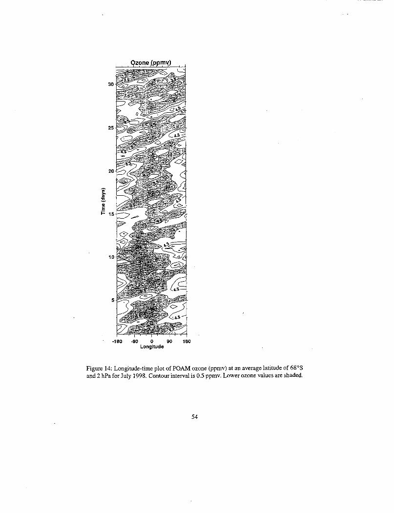
4 POAM Ozone Data

This section presents POAM (Polar Ozone and Aerosol Measurement) ozone data

(Lucke et al. 1999) that observationally validates key features of the 4-day wave as seen

in the DAO ozone assimilation. During July 1998 the POAM ozone observations were

confined between about 65-70"s and therefore will be treated as being at a constant

latitude. There are -14 ozone profiles taken each day. This does not give much resolu-

tion for a longitude time plot: nevertheless, Fig. 14 shows one attempt to interpolate the

longitude-time POAM observations at 2 hPa to a regular grid suitable for contouring

the high frequency waves. Comparing with the assimilation ozone (Fig. Ib), the POAM

observations show a similar time mean wave 1 structure and propagating wave 2 fea-

ture. The amplitude of the wave 2 signal in the POAM ozone is nearly the same as in

the DAO ozone assimilation (the contour interval is doubled in Fig. 14), although there

21

is an offset to slightly higher overall values of ozone in the POAM observations.

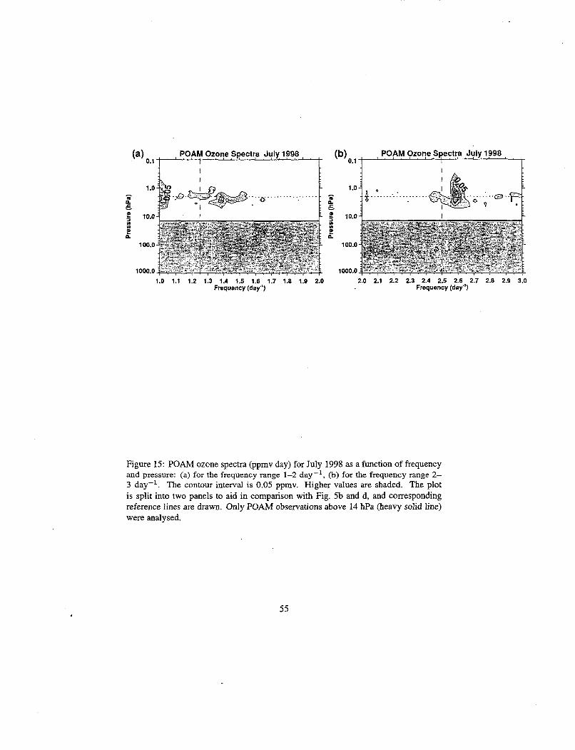
Figure 15 provides more quantitative evidence of the high frequency wave in the

POAM observations using an analysis method similar to that of Prata (1984). Here

the POAh4 observations at each level are taken as a time series for the month and a

Fourier transform is performed on the month long time series (43 1 points at each level

for the month of July 1998). This method does not separate out the wavenumber de-

pendence, however stationary waves l and 2 would correspond to l day-’ and 2 day-‘

frequencies respectively (as the Earth rotates under the satellite), and 4 day rotational

period, westward propagating waves 1 and 2 would correspond to 1.25 day-’ and

2.5 day-’ frequencies respectively (by adding the frequency of the wave motion to the

corresponding frequency associated with the Earth’s rotation). The results are plotted

in two frequency ranges (Fig. 15a and b) to aid in making comparisons with Fig. 5b

and d. Figures 15a and 15b can be interpreted as wave 1 and wave 2 plots, though this

interpretation of the POAM observations is not unique.

Spectral analysis of the POAM time series confirms what can easily be seen as

the largest signal in the time series: an oscillation near .2 hPa with a frequency of

2.58 days-‘ (Fig 15b). A stationary wave 2 would yield a peak of 2 days-‘ and an

eastward propagating wave 2 would have 2 days-’ added to its frequency, in this citse

0.58 days-’, exactly the peak seen in the DAO ozone assimilation and temperature

22

(Fig. 5). Of course, the peak at 2.58 days-l could also be produced by a very rapidly

moving eastward wave 1 or a westward propagating wave 3. However, the wave 2

interpretation seems most likely in this case, given the DAO assimilation results. Only a

portion of the POAM spectrum is shown in Fig. 15: however, the 2.58 day-' frequency

peak is by far the largest spectral peak. The magnitude of the 2.58 day-' peak is about

the same as that found in the DAO ozone spectra (fig. 5d) and the peak is located at

-2 hPa in both the POAh4 ozone spectra and the DAO ozone spectra.

'

Figure 15a shows a stationary wave 1 signal ( also apparent in Fig. 14) at 1 day-'

and a very small peak at 1.4 day-' that can be interpreted as corresponding to the small

wave 1 ozone peak seen in Fig. 5b at 0.4 day-l. As pointed out in the discussion of

Fig. 5b, this peak is near the frequency corresponding to the mean wind speed (i.e. near

the critical line).

5 Discussion

The assimilation products shown here clearly display high frequency planetary-scale

waves over the pole during the southern hemisphere winter. Issues to be discussed

concern the quality of the assimilation products for high frequency wave studies, the

ability of linear instability theory to explain the results, and the advective peaks seen in

23

I the ozone spectra.

a. Quality

The meteorological data going into the fvDAS at these levels (2 hPa) are mainly satel-

lite radiance measurements. That these observations contain the 4-day wave is not

surprising given that the early work in studying the 4-day wave (Venne and Stanford

1979, 1982; Prata 1984) was based directly on satellite radiances. The fvDAS used a

lDVAR assimilation (Joiner and Rokke 2000) of satellite radiances and should reflect

any waves in these radiances. However a good representation of the waves is needed in

the GCM as well in order for them to persist in the analysis. The ability of the fvGCM

to realistically represent these wave has not been studied to date.

The top level of the analysis may be too low to completely characterize the waves.

As mentioned in the introduction, the top analysis level is 0.4 hPa with the highest

pressure level output being slightly above it at 0.2 hPa. The negative qv region and

the wave 2 critical level extend above this altitude. It would be more satisfying if the

entire regions of unstable and high zonal wind speeds were captured. The fvGCM does

extend to 0.01 hPa so the whole region of instability may indeed be contained by the

fvDAS .

24

when the band-passed filtered temperatures did not closely resemble the warm tem-

The ozone data assimilation system was run without chemistry at this time, relying

on observations to correct for photochemical modifications. This may lead to some

biases in the mean values and wave amplitudes in the ozone assimilation, however, the

basic patterns should be captured via advection by the fvGCM coupled with the ozone

observations, since past studies have shown the 4-day wave signal in ozone (Allen

et al. 1997) and other tracer gases (Manney et al. 1998) is predominantly a transport

phenomenon. Here, the 4-day wave signal in the DAO assimilated ozone agreed well

with contemporaneous POAM ozone observations.

Band-passed filtered fields were used here because the 2-day wave signal was well-

defined and persistent throughout July 1998. Generally the band passed filtered fields

closely followed the full wave pattern (by comparison of corresponding maps, not

shown): however, there were some specific times (mainly at the end of the month)

perature regions. At these times enhanced wave 1 and wave 3 components were also

present, and thus, more spectral components or a non Fourier approach are required

taken for detailed study of the dynamical situation at these times.

The key to this study was the availability of fvDAS products every 6 hours. Such

time resolution resolves these fast propagating and fast changing waves and thus per-

mits a detailed study of their properties and evolution.

25

b. Instability theory

In linear instability theory a negative qy region is correlated with a region of EP flux

divergence. Hartmann (1983) found exact correlation in his barotropic model. In their

baroclinic model Manney and Randel (1993) also found EP flux divergence and neg-

ative 4 regions were very closely correlated. In this study, we found that regions of

EP flux divergence were not so well correlated with negative qY regions. Throughout

the month of July 1998, the EP flux divergences are closely associated with a negative

qy region, however, the negative gy regions seem to disappear quickly once a region of

EP flux divergence appears. The negative qy region is never completely eliminated, but

rather tends to shift to a different latitude or height.

Some of the wave structure seems to show wave propagation away from the source

region toward convergence at a critical level. This can be seen in Fig. 10a where the

EP flux vectors converge on the critical line at about 20 hPa. By contrast, EP flux

vectors from a linear model shown in Manney and Randel (1993) are only large close

to the negative qv region.

Fig. 2d shows how zonally asymmetric the negative potential vorticity regions can

be. This suggests that (in this example at least) formulating the problem in terms of

waves growing on a zonally symmetric unstable state may only be a first step in un-

26

derstanding the origin and evolution of the waves. All of the zonally averaged EP flux

divergence regions shown here overlap with negative potential vorticity regions at some

longitude (not shown). Additional consideration of wave-wave interactions (Manney

et al. 1989) or a more three-dimensional modelling approach may be needed.

Overall, our study supports earlier linear instability models that associate regions of

potential vorticity instability as the source of the waves. The waves propagate (where

qy is positive) more slowly than the mean wind in agreement with Rossby wave theory.

In addition the wave’s vertical scale decreases as the waves approach the critical level

from above, as seen in Fig. 9a where the phase of the geopotential height field begins

to change rapidly, again in agreement with linear Rossby wave theory. The frequency

of the wave is determined by the near coincidence of the qy = 0 line and a constant

zonal mean zonal wind line (critical line) in the region between the double jet.

c. Advective ozone peak

While the temperature spectra peak at frequencies that imply phase speeds slower than

the zonal mean zonal wind, the ozone spectra show a tendency for additional peaks

at frequencies that imply phase speeds that are faster than the zonal mean zonal wind

speed (Fig. 6) . This may imply that the wave-induced temperature response is more

27

dynamically controlled than the ozone response. Chemistry or diabatic processes may

act to create ozone gradients along pv contours allowing the wave-induced ozone re-

sponse to have a passive advection signal as well. While no signals like this were seen

in Manney et al. (1998) a large fast moving ozone peak was seen in the spectra pre-

sented in Allen et al. (1997). The results here should be interpreted with some caution

as these advective peaks were not identified prior to the spectral analysis and the rela-

tion between the spectra of advected tracers to the zonal mean zonal wind speed has

not been investigated explicitly here.

As recognized by past studies (Prata 1984; Lawrence et al. 1995), the wave temper-

ature perturbation is not simply being advected by the zonal mean zonal wind. Indeed,

our results show that the temperature perturbations are generally moving more slowly

than the mean wind. The DAO ozone assimilation results serve as a reminder that

advection is more likely to produce filaments, rather than well-defined isolated temper-

ature regions. This can be seen to some extent in Fig. 2, where the temperature map

has less filamentary structure than the corresponding ozone map.

28

6 Conclusion

This paper has focused on a month (July 1998) when the wave 2 component of the

4-day wave was well defined and persistent. The availability of 6 hourly output from

the fvDAS has allowed the first detailed global examination of this fast moving wave

feature. In addition, a companion ozone assimilation allowed identification of the high

frequency wave in the assimilated ozone field.

This wave 2 component (1.7 day period) is generally consistent with past obser-

vational studies and linear instability models. Enhanced EP flux divergence is closely

associated with negative gv regions with the wave amplitude mainly confined by the

critical line to phase speeds westward with respect to the mean flow..

The wave 2 also appears prominently in the DAO ozone assimilation, having an am-

plitude of about 0.5 ppmv or - 15% of the total ozone mixing ratio at 2 hPa. This ozone

signal is supported by independent POAM ozone mixing ratio observations. POAM

ozone time series at -70"s shows a spectral peak at 2.58 day-l that is consistent with

the assimilation results. The amplitude of the 2.58 day-' signal in POAM (Fig. 14)

is very close to the amplitude of the wave 2, 0.58 day-l signal in the DAO ozone as-

similation (Fig. 5d) and both show the ozone spectra at those frequencies peaking near

2 hpa.

29

In addition to the 4-day wave peaks, the ozone assimilation showed high frequency

peaks corresponding to advection with the zonal mean zonal wind speed. These peaks

may be related to mean advection of chemically or dibatically-induced ozone gradients

along the pv contours.

While the wave can appear fairly steady over the course of a month, the EP flux di-

vergence pattern can vary significantly over the course of a wave period as shown here

for the wave 2 component and in Randel and Lait (1991) and Lawrence and Randel

(1996) for the wave 1 component. This probably indicates that more detailed examina-

tion of these wave and their development may be possible using instantaneous pv maps.

This leaves open future studies based on assimilation products to further understand the

origin and development of high frequency polar waves.

Acknowledgment We would like to thank Stephen Eckermann for reviewing an early

draft of this work. We would also like to thank the POAM team for guidance in us-

ing the POAM ozone measurements. The work was supported in part by the Naval

Research Laboratory.

30

References

Allen, D. R., J. L. Stanford, L. S. Elson, E. F. Fishbein, L. Froidevaux, and J. W. Waters,

1997: The 4-day wave as observed from the Upper Atmosphere Research Satelite

Microwave Limb Sounder. J. Amos. Sci., 54,420434.

Andrews, D. G., J. R. Holton, and C. B. Leovy, 1987: Middle Atmosphere Dynamics.

Academic Press, 489 pp.

. Cohn, S . E., A. da Silva, 3. Guo, M. Sienkiewicz, and D. Lamich, 1998: Assessing

the effects of data selection with the DAO physical-space statistical analysis system.

Mon. Weather. Rev., 126,2913-2926.

Hartmann, D. L., 1983: Barotropic instability of the polar night jet stream. J. Amos.

Sci., 40, 817-835.

Joiner, J. and L. Rokke, 2000: Variational cloud clearing with tovs data. Quart. J. Roy.

Meteor SOC., 126,725-748.

Lait, L. R. and J. L. Stanford, 1988: Fast, long-lived features,in the polar stratosphere.

J. Amos. Sci., 45, 3800-3809.

Lawrence, B. N., G. J . Fraser, R.A. Vincent, and A. Philip, i995: The 4-day wave in

the Antarctic mesosphere. J. Geophys. Res., 100, 18899-18908.

31

Lawrence, B. N. and W. J. Randel, 1996: Variability in the mesosphere observed by

the Nimbus 6 PMR. J. Geophys. Res., 101,23475-23489.

Lucke, R. L., D. R. Korwan, R. M. Bevilacqua, J. S. Hornstein, E. P. Shettle, D. T.

Chen, M. Daehler, J. D. Lumpe, M. D. Fromm, D. Debrestian, B. Neff, M. Squire,

G. Konig-Langlo, and J. Davies, 1999: The Polar Ozone and Aerosol Measurement

(POAM) LII instrument and early validation results. J. Geophys. Res., 104, 18785-

18799.

Manney, G. L., 1991: The stratospheric 4-day wave in NMC data. J. Amos. Sci., 48,

1798-1 81 1.

Manney, G. L., T. R. Nathan, and J. L. Stanford, 1988: Barotropic strability of realistic

stratospheric jets. J. Amos. Sci., 45,2545-2555.

- 1989: Barotropic instability of basic states with a realistic jet and a wave. .I. Amos.

Sci. ,'46, 1250-1273.

Manney, G. L., Y. J. Orsolini, H. C. Pumphrey, and A. E. Roche, 1998: The 4-day

wave and transport of UARS tracers in the austral polar vortex. J. Atmos. Sci., 55,

3456-3470.

32

Manney, G. L. and W. J. Randel, 1993: Instability at the winter stratopause: A mecha-

nism for the 4-day wave. J. Amos. Sci., 50,3928-3938.

Prata, A. J., 1984: The 4-day wave. J. Amos. Sci., 41, 150-155.

Randel, W. J. and L. R. Lait, 1991: Dynamics of the 4-day wave in the Southern

Hemisphere polar stratosphere. J. Amos. Sci., 48,2496-2508.

Venne, D. E. and J. L. Stanford, 1979: Observations of a 4-day temperature wave in

the polar winter stratosphere. J. Amos. Sci., 36,2016-2019.

- 1982: An observational study of high-latitude stratospheric planetary waves in win-

ter. J. Amos. Sci., 39, 1026-1034.

Stajner, I., L. P. Riishojgaard, and R. B. Rood, 2001: The GEOS ozone data assimila-

tion system: Specification of error statistics. Q. J. R. Met. SOC., 127, 1069-1094.

33

List of Figures

1 Longitude time plot of (a) temperature (K) and (b) ozone mixing ratio

(ppmv) at 70"s and 2 hPa for July 1998. Temperature contour inter-

val is 5 K. Cooler temperatures are shaded. Ozone contour interval is

1 ppmv. Lower ozone values are shaded. . . . . . . . . . . . . . . . .

Circulation at 2 hPa on 16 July 1998 122: (a) temperature (K), tem-

41

2

peratures less than 235 K shaded, contour interval 2.5 K; (b) potential

vorticity (pvu, where 1 pvu = 1 x ~ O - ~ K m2 kg-' s-l) pv less than

-5500 pvu shaded, contour interval 500 pvu; (c) ozone @pmv), ozone

less than 2.5 ppmv shaded, contour interval 0.5 ppmv, and; (d) zonal

wind component (m s-'), qy less than zero is shaded, contour interval

10 m s-'. Orthographic projection from equator to South Pole, 90"

East at the bottom of the plots, highlighted latitude at 70" South. . . .

Time series of (a) temperature (K) and (b) ozone (ppmv) at 0" longi-

42

,. 3

tude, 70" south latitude. Time resolution is 6 hr. Altitude is 2 hPa. . . 43

34

4 Latitude-time contour plot of (a) temperature (K), 5 K contour interval,

dark shading: temperatures less than 235 K, light shading: tempera-

tures less than 245 K and @) ozone (ppmv), 1 ppmv contour interval,

shading: ozone less than 3.5 ppmv. Altitude is 2 hPa. . . . . . . . . .

July 1998 wave amplitudes as a function of frequency (cycles day-I)

and pressure at 70"s: (a) wave 1 temperature (K), (b) wave 1 ozone (ppmv),

(c) wave 2 temperature (K), and (d) wave 2 ozone (ppmv). Tempera-

ture contour interval 0.5 K. Ozone contour interval 0.05 ppmv. The

thicker solid curve plots the critical line at 70"s. The vertical dashed

lines highlight the 4 day (for wave I) and 2 day (for wave 2) frequen-

cies. The horizontal dotted line is at 2 hPa. Values below 500 hPa are

44

5

not shown. Larger amplitudes are shaded. . . . . . . . . . . . . . . . 45

35

6 July 1998 wave amplitudes as a function of frequency (cycles day-')

and latitude at 2 hPa: (a) wave 1 temperature (K), (b) wave 1 ozone (ppmv),

(c) wave 2 temperature (K), and (d) wave 2 ozone (ppmv). Tempera-

ture contour interval is 0.5 K. Ozone contour interval is 0.05 ppmv.

The thicker solid curve plots the critical line at 2 hPa. The vertical

dashed lines highlight the 4 day (for wave 1) and 2 day (for wave 2)

frequencies. The horizontal dotted line is at 70's. Larger amplitudes

are shaded. . . . . . . . . . . . . . . . . . . . . . . . . . . . . . . . 46

July 1998 wave amplitudes as a function of frequency (cycles day-')

and latitude at 0.4 hPa: (a) wave 1 potential vorticity (pvu), (b) wave 1

geopotential heights (m), (c) wave 2 potential vorticity (pvu), and (d)

wave 2 geopotential heights (m). Potential vorticity contour interval

1000 pvu. Geopotential height contour interval 50 m. The thicker

solid curve plots the critical level at 0.4 hPa. The diagonally striped

7

region denotes latitudes where qv is negative. The vertical dashed lines

highlight the 4 day (for wave 1) and 2 day (for wave 2) frequencies.

The horizontal dotted line is at 70"s. Larger amplitudes are shaded. . 47

36

8 Wave 2 structure, July 1998, 1.72 day period, as a function of latitude

and pressure. The heavy dark curve is the critical line. (a) zonal mean

zonal wind (m s-l). Shaded region is where the zonal mean pv gra-

dient, qV, is negative, Dotted reference line at 0.4 hPa (b) zonal mean

temperature (K). Thicker dashed curve is where the horizontal temper-

ature gradient is zero. Shaded region is where Qy, is negative. (c) tem-

perature wave amplitude (K, shaded contours, contour interval 0.5 K)

and phase (degrees, black lines, contour interval 45'). (d) ozone wave

amplitude (ppmv, shaded contours, contour interval 0.05 ppmv) and

phase (degrees, black lines, contour interval 45 "). Reference broken

lines at 70's and 2 hPa in (c) and (d). . . . . . . . . . . . . . . . . . 48

37

9 Wave 2 structure, July 1998, 1.72 day period, as a function of latitude

and pressure. The heavy dark curve is the critical line. (a) geopoten-

tial height wave amplitude (m, shaded contours, contour interval 10 m,

maximum contour is 80 m) and phase (degrees, black lines, contour

interval lo"). Dotted reference line at 0.4 hPa; (b) vertical velocity

amplitude ( x ~ O - ~ m s-', shaded contours, contour interval 0.1 x ~ O - ~

m s-') and phase (degrees, black lines, contour interval 20"); (c) mean

latitudinal ozone gradient (ppmv deg -' , shaded contours, contour in-

terval 0.025 ppmv deg-') and ozone wave amplitude (dashed lines)

taken from Fig. 8d; (d) zonal wind amplitude (m s-', shaded contours,

contour interval 1 m s-') and phase (degrees, black lines, contour in-

terval 30'). . . . . . . . . . . . . . . . . . . . . . . . . . . . . . . . 49

38

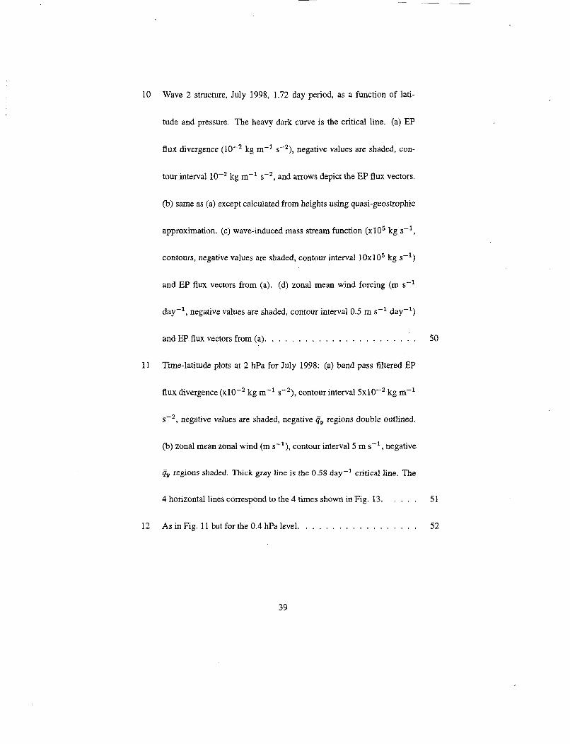
10 Wave 2 structure, July 1998, 1.72 day period, as a function of lati-

tude and pressure. The heavy dark curve is the critical line. (a) EP

flux divergence (1 0-2 kg rn-l s - ~ ), negative values are shaded, con-

kg m-l s-~, and arrows depict the EP flux vectors.

(b) same as (a) except calculated from heights using quasi-geostrophic

approximation. (c) wave-induced mass stream function (x105 kg s-',

contours, negative values are shaded, contour interval 10x105 kg s-')

and EP flux vectors from (a). (d) zonal mean wind forcing (m s-l

day-l, negative values are shaded, contour interval 0.5 m s-' day-')

tour interval

and EP flux vectors from (a). . . . . . . . . . . . . . . . . . . . . . . 50

11 Time-latitude plots at 2 hPa for July 1998: (a) band pass filtered EP

flux divergence ( x I O - ~ kg m-l s - ~ ), contour interval 5x1OU2 kg rn-l

s - ~ , negative values are shaded, negative qy regions double outlined.

(b) zonal mean zonal wind (m s-'), contour interval 5 m s-I, negative

regions shaded. Thick gray line is the 0.58 day-l critical line. The

4 horizontal lines correspond to the 4 times shown in Fig. 13. . . . . 51

12 As in Fig. 11 but for the 0.4 hPa level. . . . . . . . . . . . . . . . . . 52

39

13 Plots of EP flux divergence (left, contour interval 2.5~10-~ kg rn-l

s - ~ , negative values are shaded) and zonal mean zonal wind (right,

contour interval 10 m s-l) at four times during July 1998. EP flux

vectors are scaled to be 40% smaller than in Fig. 10 to aid readability.

The heavy line on the right is the critical line for a 1.72 day period

wave 2 mode. Negative 4 regions are shaded on the right and qv = 0

are double lines on the left. . . . . . . . . . . . . . . . . . . . . . . . 53

14 Longitude-time plot of POAM ozone (ppmv) at an average latitude of

68"s and 2 hPa for July 1998. Contour interval is 0.5 ppmv. Lower

ozone values are shaded. . . . . . . . . . . . . . . . . . . . . . . . . 54

15 POAM ozone spectra (ppmv day) for July 1998 as a function of fre-

quency and pressure: (a) for the frequency range 1-2 day-', (b) for

the frequency range 2-3 day-'. The contour interval is 0.05 ppmv.

Higher values are shaded. The plot is split into two panels to aid in

comparison with Fig. 5b and d, and corresponding reference lines are

drawn. Only POAM observations above 14 hPa (heavy solid line) were

analysed. . . . . . . . . . . . . . . . . . . . . . . . . . . . . . . . . 55

40

30

25

20

2.

s

i= 15 2

10

5

30

25

20

h

2. m s

i= 15 E

i o

r

-180 -90 0 90 180 Longitude

-180 -90 0 90 180 Longitude

Figure 1: Longitude time plot of (a) temperature (K) and (b) ozone mixing ratio (ppmv) at 70"s and 2 hPa for July 1998. Temperature contour interval is 5 K. Coolei :empe:2- tures are shaded. Ozone contour interval is 1 ppmv. Lower ozone values are shaded.

41

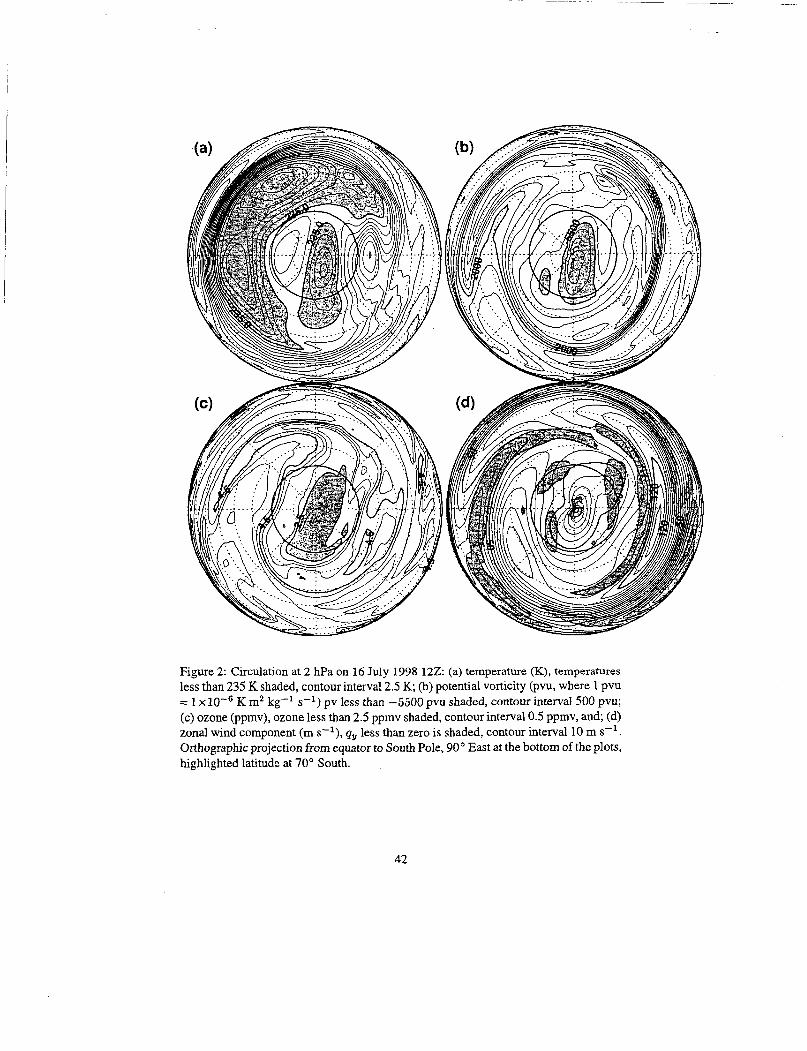
Figure 2: Circulation at 2 hPa on 16 July 1998 122: (a) temperature (K), temperatures less than 235 K shaded, contour interval 2.5 K, (b) potential vorticity (pvu, where 1 pvu = 1 x K m2 kg-' s-l) pv less than -5500 pvu shaded, contour interval 500 pvu; (c) ozone (ppmv), ozone less than 2.5 ppmv shaded, contour interval 0.5 ppmv, and; (d) zonal wind component (m s-l), qy less than zero is shaded, contour interval 10 m s-'. Orthographic projection from equator to South Pole, 90" East at the bottom of the plots, highlighted latitude at 70" South.

,

42

P v

I-

01 Apr 101 May (01 Jun

280

270

260

250

240

230

220

01 Jul (01 Aug 01 Sep

01 Apr 101 May

n

01 Jun 101 Jul 01 Aug 101 Sep

Figure 3: Time series of (a) temperature (K) and @) ozone (ppmv) at 0" longitude, 70" south latitude. Time resolution is 6 hr. Altitude is 2 hPa.

43

01 Apr 101 May (01 Jun (01 Jul (01 Aug 1998

01 Apr (01 May (01 Jun (01 Jul 01 Aug (01 Sep

Figure 4: Latitude-time contour plot of (a) temperature (K), 5 K contour interval, dark shading: temperatures less than 235 K, light shading: temperatures less than 245 K and @) ozone (ppmv), 1 ppmv contour interval, shading: ozone less than 3.5 ppmv. Altitude is 2 hPa.

44

0.1 (b)

0.1 (a)

1 .o 1 .o ................. - .......... A

a 5. z g 10.0 g 10.0 n n

e e! a a 100.0 100.0

1000.0 1000.0

0.0 0.1 0.2 0.3 0.4 0.5 0.6 0.7 0.8 0.9 1.0 Eastward Frequency (day.') Eastward Frequency (day")

0.1 (a

1 .o - . . . . . . . ..a -0 2 c,

10.0 ; e n

100.0

1000.0

0.0 0.1 0.2 0.3 0.4 0.5 0.6 0.7 0.8 0.9 1.0 0.0 0.1 0.2 0.3 0.4 0.5 0.6 0.7 0.8 0.9 1.0 Eastward Frequency (day") Eastward Frequency (day")

Figure 5: July 1998 wave amplitudes as a function of frequency (cycles day-') and pressure at 7OOS: (a) wave 1 temperature (K), (b) wave 1 ozone (ppmv), (c) wave 2 temperature (K), and (d) wave 2 ozone (ppmv). Temperature contour interval 0.5 K. Ozone contour interval 0.05 ppmv. The thicker solid curve plots the critical line at 70"s. The vertical dashed lines highlight the 4 day (for wave 1) and 2 day (for wave 2) frequencies. The horizontal dotted line is at 2 hPa. Values below 500 hPa are not shown. Larger amplitudes are shaded.

45

Wave 1 :,Temperature (K) I ' O I ' " " '

I

-30 -30 al a, U 0

L L - I - - -I

-60 -60

_... _........ ..

-90 -90

0.0 0.1 0.2 0.3 0.4 0.5 0.6 0.7 0.8 0.9 1.0 Eastward Frequency (day")

Wave 2: Temperature (K) I

I I -30

m U - e .- -I

-60

- g o { , , , , , , , I , , , , , ! 0.0 0.1 0.2 0.3 0.4 0.5 0.6 0.7 0.8 0.9 1.0

Eastward Frequency (day")

0.0 0.1 0.2 0.3 0.4 0.5 0.6 0.7 0.8 0.9 1.0 Eastward Frequency (day")

(d) 0

-30 al 0

Io -I I e .-

-60

-90

0.0 0.1 0.2 0.3 0.4 0.5 0.6 0.7 0.8 0.9 1.0 Eastward Frequency (day")

Figure 6: July 1998 wave amplitudes as a function of frequency (cycles day-') and latitude at 2 hPa: (a) wave 1 temperature (K), (b) wave 1 ozone (ppmv), (c) wave 2 temperature (K), and (d) wave 2 ozone (ppmv). Temperature contour interval is 0.5 K. Ozone contour interval is 0.05 ppmv. The thicker solid curve plots the critical line at 2 hPa. The vertical dashed lines highlight the 4 day (for wave 1) and 2 day (for wave 2 ) frequencies. The horizontal dotted line is at 70"s. Larger amplitudes are shaded.

46

Wave 1 : PV (pvu) (a) 0 " " ' i " " " " " ' I . ' i

I

0.0 0.1 0.2 0.3 0.4 0.5 0.6 0.7 0.8 0.9 1.0 Eastward Frequency (day")

Wave 2: P V (pvu), ( C ) O ' " . ' ' . ' , ' ' " " "

I

-30 0 0

e e .- 2

-60

-90 I , , , , , , , I ' I 0.0 0.1 0.2 0.3 0.4 0.5 0.6 0.7 0.8 0.9 1.0

Eastward Frequency (day")

-30 a, U .- e .- d

-60

..................

-90 '0.0 0.1 0.2 0.3 0.4 0.5 0.6 0.7 0.8 0.9 1.0

Eastward Frequency (day") Wave 2: Z (m) ( d ) O ' ' ' ~ ' " ' i

I I -30

a, 0 - .- - 111 -I

-60

.......................

- 9 0 1 , , , , , I , , , , , I 0.0 0.1 0.2 0.3 0.4 0.5 0.6 0.7 0.8 0.9 1.0

Eastward Frequency (day")

Figure 7: July 1998 wave amplitudes as a function of frequency (cycles day-') and latitude at 0.4 hPa: (a) wave 1 potential vorticity (pvu), (b) wave 1 geopoten- tial heights (m), (c) wave 2 potential vorticity (pvu), and (d) wave 2 geopotential heights (m). Potential vorticity contour interval 1000 pvu. Geopotential height contour interval 50 m. The thicker solid curve plots the critical level at 0.4 hPa. The diagonally striped region denotes latitudes where rjv is negative. The vertical dashed lines high- light the 4 day (for wave 1) and 2 day (for wave 2) frequencies. The horizontal dotted line is at 70's. Larger amplitudes are shaded.

47

-90 -80 -70 -60 -50 -40 -30 -90 -80 -70 -60 -50 -40 -30 Latitude Latitude

Wave 2: Ozone (ppmv) 0.1 i Wave 2: T (K) (dl

0.11 " ' i " " i (c) I I

. - - I 1.0- I 1.0-

5 .. . . . .... . - r . e a en

P P

n e 10.0; i z 10.0-

- .. . . . . . . . .

E

l , I

100.0 , ,

-90 -80 -70 -60 -50 -40 -30 Latitude Latitude

100.0 -90 -80 -70 -60 -50 -40 -30

Figure 8: Wave 2 structure, July 1998, 1.72 day period, as a function of latitude and pressure. The heavy dark curve is the critical line. (a) zonal mean zonal wind (m s-l). Shaded region is where the zonal mean pv gradient, qy, is negative. Dotted reference line at 0.4 hPa (b) zonal mean temperature (IC). Thicker dashed curve is where the horizontal temperature gradient is zero. Shaded region is where (fy, is negative. (c) temperature wave amplitude (K, shaded contours, contour interval 0.5 K) and phase (degrees, black lines, contour interval 45"). (d) ozone wave amplitude (ppmv, shaded contours, contour interval 0.05 ppmv) and phase (degrees, black lines, contour interval 45'). Reference broken lines at 70's and 2 hPa in (c) and (d).

48

J

. . . . . . . . . 0 v i - m 1.0- - m 1.0-

e - E 2 m

2 - g

g 10.0- g 10.0- In

7

100.0

-90 -80 -70 - 4 0 -50 -40 -30 Latitude

Wave 2: 0, Grad (ppmv deg-') (c)

100.0 -90 -80 -70 -60 -50 -40 -30

Latitude Wave 2: u (rn d) (d)

g 1.0 g 1.0- L

: 10.0 E l0.Oj -

5 E

5 t 7 m

100.0 100.0 i -90 -80 -70 -60 -50 -40 -30 -90 -80 -70 -60 -50 -40 -30

Latitude Latitude

Figure 9: Wave 2 structure, July 1998, 1.72 day period, as a function of latitude and pressure. The heavy dark curve is the critical line. (a) geopotential height wave ampli- tude (m, shaded contours, contour interval 10 m, maximum contour is 80 m) and phase (degrees, black lines, contour interval loo). Dotted reference line at 0.4 hPa; (b) ver- tical velocity amplitude ( X ~ O - ~ m s-l, shaded contours, contour interval 0.1 x ~ O - ~ m s-l) and phase (degrees, black lines, contour interval 20"); (c) mean latitudinal ozone gradient (ppmv deg-l, shaded contours, contour interval 0.025 ppmv deg-') and ozone wave amplitude (dashed lines) taken from Fig. 8d; (d) zonal wind amplitude (m s-l, shaded contours, contour interval 1 m s-l) and phase. (degrees, black lines, contour interval 30").

49

(4 Wave 2: EP flux div (lO-',kg rn-' s-') ,

m 1.0- n E. 5 0)

m

$ 10.0-

100.0 -90 -80 -70 -60 -50 -40 -30

Latitude Wave 2: Stream Function, (IO5 kq s-') ,

I 0.1 i ' (a

(b) , Wave 2: QG,EP flux div (10' kg m;l s-') , 0.1 I ' I

I- . r- 100.0

-90 -80 -70 -60 -50 -40 -30 Latitude

(a Wave 2: EP flux< div (rn ,s-' day-') I

- 1.0 n m 1.0 n 5 5 e 2

- m al

m

d 10.0 g 10.0

100.0 100.0

-90 -80 -70 -60 -50 -40 -30 . Latitude

Figure 10: Wave 2 structure, July 1998, 1.72 day period, as a function of latitude and pressure. The heavy dark curve is the critical line. (a) EP flux divergence (lo-' kg rn-l s-~), negative values are shaded, contour interval lo-' kg rn-l s-~, and ar- rows depict the EP flux vectors. (b) same as (a) except calculated from heights using quasi-geostrophic approximation. (c) wave-induced mass stream function (xl O5 kg s-l, contours, negative values are shaded, contour interval 10x105 kg s-') and EP flux vectors from (a). (d) zonal mean wind forcing (m s-I day-', negative values are shaded, contour interval 0.5 m s-l day-') and EP flux vectors from (a). .

50

30

25

20

h u)

m I!

F 15 E

10

5

30

25

20

h

5. m I!

i= 15 E

i a

5

-90 -80 -70 -60 -50 -40 -30 Latitude

-90 -80 -70 -60 -50 -40 -30 Latitude

Figure 11: Time-latitude plots at 2 hPa for July 1998: (a) band pass filtered EP flux divergence ( x ~ O - ~ kg m-l s - ~ ) , contour interval 5x10F2 kg m-' s - ~ , negative values are shaded, negative qV regions double outIined. (b) zonal mean zonal wind (m s-'), contour interval 5 m s-', negative qv regions shaded. Thick gray line is the 0.58 day-' critical line. The 4 horizontal lines correspond to the 4 times shown in Fig. 13.

51

3c

L

25

20

n v)

5. a E E F 15

10

5

I -90 -80 -70 -60 -50 -40 -30

Latitude

30

25

20

n

s

F 15 E

10

5

-90 -80 -70 -60 -50 -40 -30 Latitude

Figure 12: As in Fig. 11 but for the 0.4 hPa level.

52

- 1 0

d D I

100

1W 0 -W JO -70 50 do 4 0 Jo

L&d. EP flux div(l0'kg rn: r? 13 +ly,l@9p 182 (c) , , 0.1

-. .

- 1 0 c - I i - 100

1000

1.0

: 6

100

1000

- 1.0

z D - 10.0

lW.O

- 1.0 c I 2 i

-

10.0

1m.o

Figure 13: Plots of EP flux divergence (left, contour interval 2 . 5 ~ 1 0 - ~ kg m-l s - ~ , negative values are shaded) and zonal mean zonal wind (right, contour interval 10 m s-l) at four times during July 1998. EP'flux vectors are scaled to be -10% smaller than in Fig. 10 to aid readability. The heavy line on the right is the critical line for a 1.72 day period wave 2 mode. Negative c&, regions are shaded on the right and qv = 0 are double lines on the left.

53

30

25

20

10

5

-180 -90 0 90 180 Longitude

Figure 14: Longitude-time plot of POAh4 ozone (ppmv) at an average latitude of 68"s and 2 hPa for July 1998. Contour interval is 0.5 ppmv. Lower ozone values are shaded.

54

. 7

e e a a u)

100.0 100.0

1000.0 1000.0 1.0 1.1 1.2 1.3 1.4 1.5 1.6 1.7 1.0 1.9 2.0 2.0 2.1 2.2 2.3 2.4 2.5 2.6 2.7 2.8 2.9 3.0

Frequency (day") Frequency (day")

Figure 15: POAM ozone spectra (ppmv day) for July 1998 as a function of frequency and pressure: (a) for the frequency range 1-2 day-', (b) for the frequency range 2- 3 day-'. The contour interval is 0.05 ppmv. Higher values are shaded. The plot is split into two panels to aid in comparison with Fig. 5b and d, and corresponding reference lines are drawn. Only POAM observations above 14 hPa (heavy solid line) were analysed.

55