Solar Backscatter Ultraviolet Instrument (SBUV/2) Version 8 Ozone Retrieval Algorithm Theoretical Basis Document (V8 ATBD) Edited by L. Flynn (Last Revision February 2, 2007) Background

The Solar Backscatter Ultraviolet (SBUV/2) instruments are the operational ozone- monitoring satellite instruments for the U.S.. They are flown on NOAA’s Polar-orbiting Operational Environmental Satellites (POES). The new Version 8 algorithms are being implemented for operational processing and reprocessing of NOAA’s SBUV(/2) measurements to produce total column and vertical profile ozone estimates. Versions of the total ozone component of this algorithm are used with EP-TOMS and EOS Aura OMI measurements. Purpose

This ATBD presents a description of the theory and science in the Version 8 total ozone algorithm (V8T) and the Version 8 ozone profile algorithm (V8P) as applied to SBUV/2 instrument measurements. The V8T is very similar to the improved Version 8 of the NASA Total Ozone Mapping Spectrometer (TOMS) total ozone column algorithm with modifications for differences in the measurements. The first two chapters of this document reproduce large sections of the TOMS Version 8 ATBD (by P.K. Bhartia and C.G. Wellemeyer) and the Ozone Monitoring Instrument (OMI) ATBD Volume II: OMI Ozone Products (edited by P.K. Bhartia) with changes for the operational and reprocessing SBUV/2 implementations. The third chapter describes the V8P with emphasis on differences and improvements between it and the previous Version 6 SBUV/2 ozone profile retrieval algorithm.

Chapter 1: Scientific Overview

1.1 Introduction This chapter describes the theoretical basis of the measurements used in the Version 8

algorithms (V8). V8 is the most recent version of the backscattered ultraviolet (BUV) algorithms that have undergone three decades of progressive refinement. Its predecessors, V7 for total ozone, developed about in 1998, and V6 for profile ozone, developed in about 1990, have been used to produce the acclaimed TOMS total ozone and SBUV(/2) ozone profile time series. V8 will correct several small errors in V7 and V6 that were discovered by extensive error studies using radiative transfer models and by comparison with ground-based instruments. The V8T uses only two wavelengths (318 nm and 331 nm) to derive total ozone. Other wavelengths are used for diagnostics and error correction. Experience with TOMS and SBUV/2 suggests that the algorithm is capable of producing total ozone with rms error of about 2%, though these errors are not necessarily randomly distributed over the globe. The errors typically increase with solar zenith angle and in presence of heavy aerosol loading.

The SBUV/2 instruments provide measurements of Earth's total column ozone by measuring the backscattered Earth radiance at a set of discrete 1.1-nm wavelength bands. Both ozone-absorbing and non-absorbing regions of the BUV spectrum are sampled, and the concept of differential absorption is used to derive total column ozone from these measurements. The experiments use a double monochromator and a grating drive to sample the BUV radiation at nadir in 12 discrete wavelength channels over 24 seconds. A second detector, called the cloud cover radiometer, makes measurements of the BUV radiation at 380 nm, with a 3-nm bandpass,

coincident with each of these monochromator measurements. The SBUV/2 uses periodic measurements of the sun to provide normalization of the BUV radiances to solar output, and to remove some instrument dependence. The SBUV/2 instruments measure radiance and irradiance with the same optical system. The SBUV/2 instruments cover 14 nadir tracks on the daylight portions of each day’s orbits. The sun synchronous near-polar orbits provide these measurements at the same approximate local time on a monthly basis, but this varies as the local equator crossing time changes with long-term orbit drifts.

Ozone profiles and total column amounts are derived from the ratio of the observed backscattered spectral radiance to the incoming solar spectral irradiance. This ratio is referred to as the backscattered albedo. The only difference in the optical components between the radiance and irradiance observations is the instrument diffuser used to make the solar irradiance measurement; the remaining optical components are identical. Therefore, a change in the diffuser reflectivity will result in an apparent trend in ozone. This is the key calibration component for the SBUV(/2) series. An on-board calibration system using direct and diffuser views of a Hg lamp provides the baseline for long-term instrument characterization. This allows one to track reflectivity changes to get accurate albedo calibration. A more detailed instrument description is available at http://www2.ncdc.noaa.gov/docs/klm/ in the NOAA KLM User’s Guide. See Hilsenrath et al. [1995] for a longer discussion on calibration.

This document is organized as follows. The next sections of this chapter provide an overview of key properties of backscattered ultraviolet radiation in the wavelength range used to derive total column and vertical profile ozone, the following chapter describes the theoretical basis of the V8T, including an error analysis, and the third chapter describes the V8P.

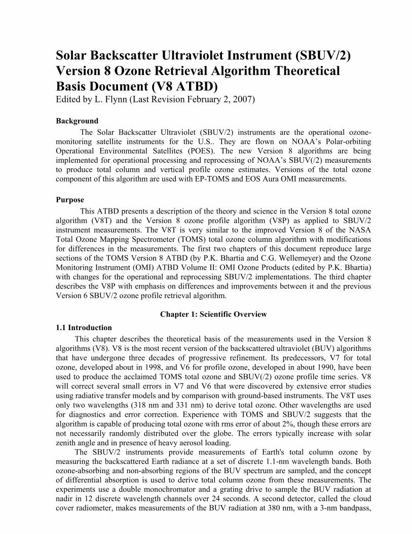
Figure 1-1a (Left) & 1-1b (Right): Ozone Absorption Cross-Sections for 250 nm to 330 nm.

1.2 Properties of Backscattered UV (BUV) Radiation The SBUV/2 instruments measure the radiation backscattered by the Earth’s atmosphere

and surface at discrete wavelengths in the range 250 nm to 380 nm. Though ozone has absorption over this entire wavelength range (Fig. 1-1a and Fig 1-1.b), the ozone profile products are retrieved by using wavelengths between 250 nm and 310 nm, where the absorption limits the penetration into the stratosphere; and the total ozone products are derived using UV wavelengths, between 310 nm and 331 nm, where the absorption is significant enough to permit reliable retrievals, but not so large that the they are absorbed before sensing most of the ozone layer. Longer wavelengths are used to identify aerosols and clouds. In the following sub-sections

we summarize key properties of the BUV radiation in the 250 nm to 380 nm wavelength range that form the basis for the algorithms described in the subsequent chapters.

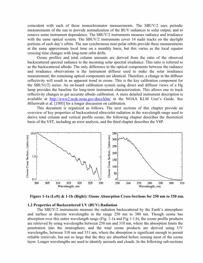
Figure 1-2: Radiance Contribution Functions for selected UV channels

1.2.1 O3 Absorption By multiplying the ozone cross-sections given in Fig. 1-1 with typical O3 column density

of 1x1019

molecule/cm2, one gets the vertical absorption optical depth of the atmosphere, which

varies from 160 at 250 nm to 0.01 at 340 nm. Since 90% of this absorption occurs in the stratosphere, little radiation reaches the troposphere at wavelengths shorter than 295 nm, hence the radiation emanating from the Earth at these wavelengths is unaffected by clouds, tropospheric aerosols, and the surface. Therefore, the short wavelength BUV radiation consists primarily of Rayleigh-scattered radiation from the molecular atmosphere, with small contributions by scattering from stratospheric aerosols [Torres & Bhartia, 1995], polar stratospheric clouds (PSC) [Torres et al., 1992], polar mesospheric clouds (PMC) [Thomas, 1984]; and emissions from NO [McPeters, 1989], Mg

++

and other ionized elements. Ozone absorption controls the depth from which the Rayleigh-scattered radiation emanates. As shown in Fig. 1-2, this occurs over a fairly broad region of the atmosphere (roughly 16-km wide at the half maximum point) defined by the radiance contribution functions (RCF). As shown by Bhartia et al. [1996], the magnitude of the BUV radiation is proportional to the pressure at which the contribution function peaks, which occurs roughly at an altitude where the slant ozone absorption optical path is approximately 1. This means that the basic information in BUV radiation is on the ozone column density as a function of pressure.

Figure 1-2 also shows that the RCF becomes extremely broad at around 300 nm with two distinct peaks; one in the stratosphere the other in the troposphere. At longer wavelengths the stratospheric peak subsides and the tropospheric peak grows. Since roughly 95% of the ozone column is above the tropospheric peak, the radiation emanating from the troposphere essentially senses the entire ozone column, while the radiation emanating from the stratosphere senses the column above the RCF peak. Thus the longer wavelengths (>310 nm) are suitable for measuring total ozone and the shorter (<310 nm) are suitable for measuring the vertical distribution of ozone profiles.

The magnitude of the BUV radiation that emanates from the troposphere is determined by molecular, cloud, and aerosol scattering, reflection from the surface, and absorption by aerosol and other trace gases. Basic information about each of these is provided in the following sections.

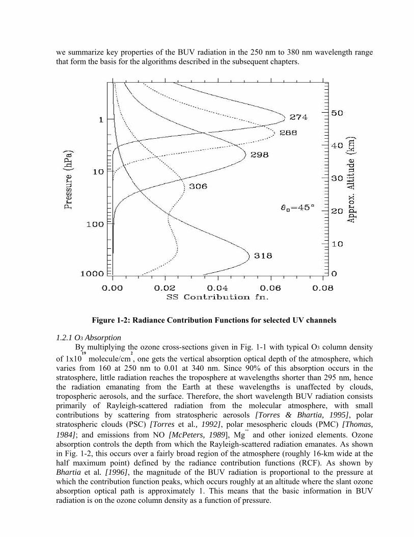
Figure 1-3: Fractional change in BUV radiance due to Ring Effect.

1.2.2 Molecular Scattering In absence of clouds, Rayleigh scattering from the molecular atmosphere forms the

dominant component of radiation measured by satellites in the 250 nm to 380 nm wavelength range. Using the standard definition [Young, 1981], we define Rayleigh scattering as consisting of conservative scattering as well as non-conservative scattering, the latter consisting primarily of rotational Raman scattering (RRS) from O2 and N2 molecules [Kattawar et al., 1981, Chance et al., 1997]. Though molecular scattering varies smoothly with wavelength, following the well-known λ

−α law (where α is approximately 4.3 near 300 nm), RRS, which contributes ~3.5 % to

the total scattering, introduces a complex structure in the BUV spectrum by filling-in (or depleting) structures in the atmospheric radiation, producing the so-called Ring Effect [Grainger & Ring, 1962] (See Fig. 1-3.). The most prominent structures in BUV radiation are those due to solar Fraunhofer lines, however, structures produced by absorption by ozone and other molecules (principally volcanic SO2) in the earth’s atmosphere are also altered by RRS. (Vibrational Raman scattering from water molecules can also produce the Ring effect. Although this effect is insignificant below 340 nm, it can be important at longer wavelengths.) Radiative

transfer codes have been developed recently [Joiner et al., 1995; Vountas et al., 1998] that calculate the effect of gaseous absorption, surface reflection and multiple scattering on the Ring signal. These models show that the fractional Ring Effect (i.e., fractional increase or decrease in BUV radiation due to RRS) is a complex, non-linear function of surface albedo, aerosol properties, and cloud optical depth, and is also affected by cloud height [Joiner & Bhartia, 1995]. These effects must be accounted for in developing the ozone retrieval algorithms. 1.2.3 Trace Gas Absorption

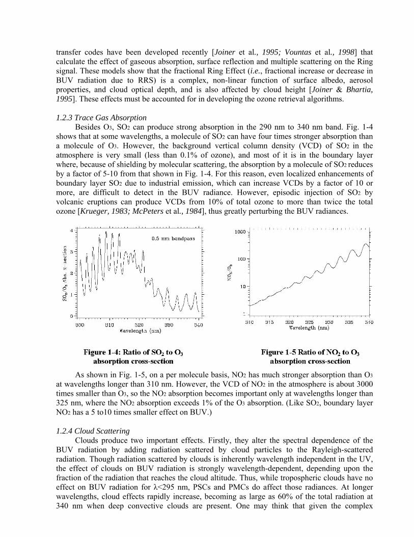
Besides O3, SO2 can produce strong absorption in the 290 nm to 340 nm band. Fig. 1-4 shows that at some wavelengths, a molecule of SO2 can have four times stronger absorption than a molecule of O3. However, the background vertical column density (VCD) of SO2 in the atmosphere is very small (less than 0.1% of ozone), and most of it is in the boundary layer where, because of shielding by molecular scattering, the absorption by a molecule of SO2 reduces by a factor of 5-10 from that shown in Fig. 1-4. For this reason, even localized enhancements of boundary layer SO2 due to industrial emission, which can increase VCDs by a factor of 10 or more, are difficult to detect in the BUV radiance. However, episodic injection of SO2 by volcanic eruptions can produce VCDs from 10% of total ozone to more than twice the total ozone [Krueger, 1983; McPeters et al., 1984], thus greatly perturbing the BUV radiances.

As shown in Fig. 1-5, on a per molecule basis, NO2 has much stronger absorption than O3

at wavelengths longer than 310 nm. However, the VCD of NO2 in the atmosphere is about 3000 times smaller than O3, so the NO2 absorption becomes important only at wavelengths longer than 325 nm, where the NO2 absorption exceeds 1% of the O3 absorption. (Like SO2, boundary layer NO2 has a 5 to10 times smaller effect on BUV.) 1.2.4 Cloud Scattering

Clouds produce two important effects. Firstly, they alter the spectral dependence of the BUV radiation by adding radiation scattered by cloud particles to the Rayleigh-scattered radiation. Though radiation scattered by clouds is inherently wavelength independent in the UV, the effect of clouds on BUV radiation is strongly wavelength-dependent, depending upon the fraction of the radiation that reaches the cloud altitude. Thus, while tropospheric clouds have no effect on BUV radiation for λ<295 nm, PSCs and PMCs do affect those radiances. At longer wavelengths, cloud effects rapidly increase, becoming as large as 60% of the total radiation at 340 nm when deep convective clouds are present. One may think that given the complex

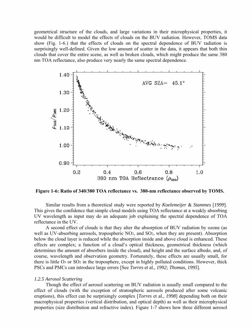
geometrical structure of the clouds, and large variations in their microphysical properties, it would be difficult to model the effects of clouds on the BUV radiation. However, TOMS data show (Fig. 1-6.) that the effects of clouds on the spectral dependence of BUV radiation is surprisingly well-defined. Given the low amount of scatter in the data, it appears that both thin clouds that cover the entire scene, as well as broken clouds, which might produce the same 380 nm TOA reflectance, also produce very nearly the same spectral dependence.

Figure 1-6: Ratio of 340/380 TOA reflectance vs. 380-nm reflectance observed by TOMS.

Similar results from a theoretical study were reported by Koelemeijer & Stammes [1999]. This gives the confidence that simple cloud models using TOA reflectance at a weakly absorbing UV wavelength as input may do an adequate job explaining the spectral dependence of TOA reflectance in the UV.

A second effect of clouds is that they alter the absorption of BUV radiation by ozone (as well as UV-absorbing aerosols, tropospheric NO2, and SO2, when they are present). Absorption below the cloud layer is reduced while the absorption inside and above cloud is enhanced. These effects are complex; a function of a cloud’s optical thickness, geometrical thickness (which determines the amount of absorbers inside the cloud), and height and the surface albedo, and, of course, wavelength and observation geometry. Fortunately, these effects are usually small, for there is little O3 or SO2 in the troposphere, except in highly polluted conditions. However, thick PSCs and PMCs can introduce large errors [See Torres et al., 1992; Thomas, 1995]. 1.2.5 Aerosol Scattering

Though the effect of aerosol scattering on BUV radiation is usually small compared to the effect of clouds (with the exception of stratospheric aerosols produced after some volcanic eruptions), this effect can be surprisingly complex [Torres et al., 1998] depending both on their macrophysical properties (vertical distribution, and optical depth) as well as their microphysical properties (size distribution and refractive index). Figure 1-7 shows how three different aerosol

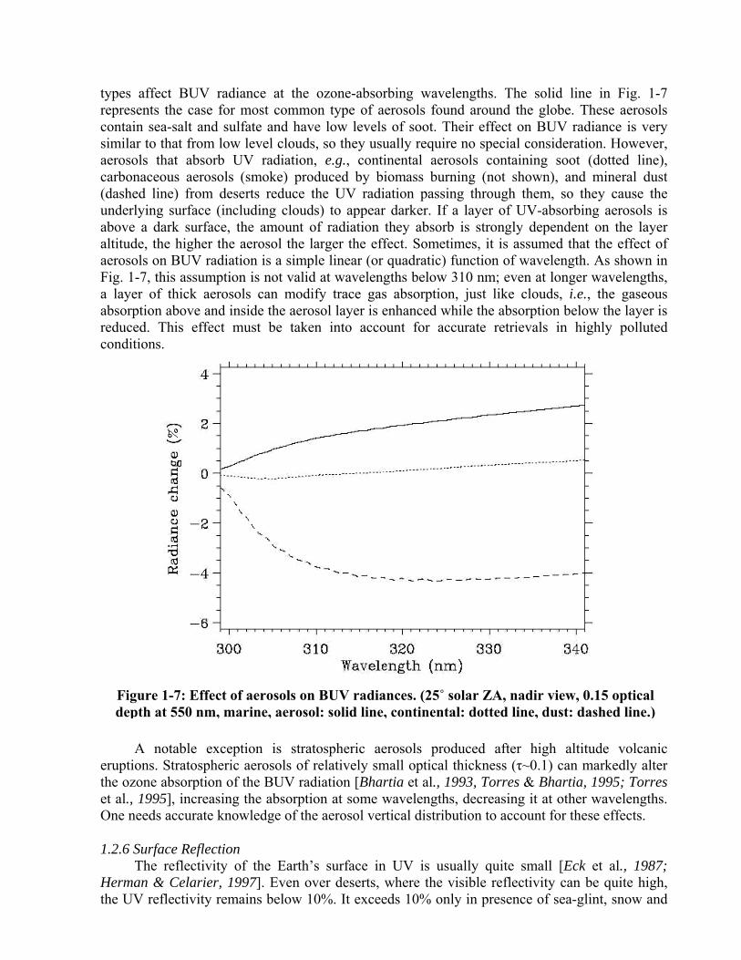
types affect BUV radiance at the ozone-absorbing wavelengths. The solid line in Fig. 1-7 represents the case for most common type of aerosols found around the globe. These aerosols contain sea-salt and sulfate and have low levels of soot. Their effect on BUV radiance is very similar to that from low level clouds, so they usually require no special consideration. However, aerosols that absorb UV radiation, e.g., continental aerosols containing soot (dotted line), carbonaceous aerosols (smoke) produced by biomass burning (not shown), and mineral dust (dashed line) from deserts reduce the UV radiation passing through them, so they cause the underlying surface (including clouds) to appear darker. If a layer of UV-absorbing aerosols is above a dark surface, the amount of radiation they absorb is strongly dependent on the layer altitude, the higher the aerosol the larger the effect. Sometimes, it is assumed that the effect of aerosols on BUV radiation is a simple linear (or quadratic) function of wavelength. As shown in Fig. 1-7, this assumption is not valid at wavelengths below 310 nm; even at longer wavelengths, a layer of thick aerosols can modify trace gas absorption, just like clouds, i.e., the gaseous absorption above and inside the aerosol layer is enhanced while the absorption below the layer is reduced. This effect must be taken into account for accurate retrievals in highly polluted conditions.

Figure 1-7: Effect of aerosols on BUV radiances. (25˚ solar ZA, nadir view, 0.15 optical depth at 550 nm, marine, aerosol: solid line, continental: dotted line, dust: dashed line.)

A notable exception is stratospheric aerosols produced after high altitude volcanic eruptions. Stratospheric aerosols of relatively small optical thickness (τ~0.1) can markedly alter the ozone absorption of the BUV radiation [Bhartia et al., 1993, Torres & Bhartia, 1995; Torres et al., 1995], increasing the absorption at some wavelengths, decreasing it at other wavelengths. One needs accurate knowledge of the aerosol vertical distribution to account for these effects.

1.2.6 Surface Reflection

The reflectivity of the Earth’s surface in UV is usually quite small [Eck et al., 1987; Herman & Celarier, 1997]. Even over deserts, where the visible reflectivity can be quite high, the UV reflectivity remains below 10%. It exceeds 10% only in presence of sea-glint, snow and

ice. More importantly, to the best of our knowledge, the UV reflectivity doesn’t vary with wavelength significantly enough to alter the spectral dependence of the BUV radiation. An important exception is the sea-glint. Since the reflectivity of the ocean, when viewed in the glint (geometrical reflection) direction, is very different for direct and diffuse light (exceeding 100% for direct when the ocean is calm, but only 5% for diffuse), in the UV, where the ratio of diffuse to direct radiation has a strong spectral dependence, the ocean appears “red”, i.e., it gets brighter as the wavelength increases. The reflectivity of the ocean at any wavelength, as well as its spectral dependence, is a strong function of wind speed, and of course, aerosol and cloud amount. Accurate retrieval in presence of sea glint requires that one account for these complex effects. Fortunately, the nadir-viewing geometry of the SBUV/2 and spacecraft orbits with equator crossing times more than an hour from solar noon limit the occurrence of sea-glint observing geometries. 1.3 References Bhartia, P.K., et al., “Effect of Mount Pinatubo Aerosols on Total Ozone Measurements From

Backscatter Ultraviolet (BUV) Experiments,” J. Geophys. Res., 98, 18547-18554, 1993. Bhartia, P.K., et al., “Algorithm for the Estimation of Vertical Ozone Profile from the

Backscattered Ultraviolet (BUV) Technique,” J. Geophys. Res., 101, 18793-18806, 1996. Chance, K., & R.J.D. “Spurr, Ring Effect Studies: Rayleigh Scattering, Including Molecular

Parameters for Rotational Raman Scattering, and the Fraunhofer Spectrum,” Applied Optics 36, 5224-5230, 1997.

Eck, T.F., et al., “Reflectivity of the Earth's Surface and Clouds in Ultraviolet from Satellite Observations,” J. Geophys. Res., 92, 4287, 1987.

Grainger, J.F. & J. Ring, “Anomalous Fraunhofer line profiles”, Nature, 193, 762, 1962. Herman, J.R., and E.A. Celarier, “Earth surface reflectivity climatology at 340-380 nm from

TOMS data,” J. Geophys. Res.,102, 28003-28011, 1997. Joiner, J., et al., “Rotational-Raman Scattering (Ring Effect) in Satellite Backscatter Ultraviolet

Measurements,” Appl. Opt., 34, 4513-4525, 1995. Joiner, J. & P.K. Bhartia, “The Determination of Cloud Pressures from Rotational-Raman

Scattering in Satellite Backscatter Ultraviolet Measurements,” J. Geophys. Res.,100, 23019-23026, 1995.

Kattawar, G.W., A.T. Young, & T.J. Humphreys, “Inelastic scattering in planetary atmospheres. I. The Ring Effect, without aerosols,” Astrophys. J., 243, 1049-1057, 1981.

Koelemeijer, R.B.A., & P. Stammes, “Effects of clouds on ozone column retrieval from GOME UV measurements,” J. Geophys. Res., 104, 8,281-8,294, 1999.

Krueger, A.J., “Sighting of El Chichon Sulfur Dioxide with the Nimbus-7 Total Ozone Mapping Spectrometer,” Science, 220, 1377-1378, 1983.

McPeters, R D., D.F. Heath, & B.M. Schlesinger, “Satellite observation of SO2 from El Chichon: Identification and Measurement,” Geophys Res. Lett., 11, 1203-1206, 1984.

McPeters, R.D., “Climatology of Nitric Oxide in the upper stratosphere, mesosphere, and thermosphere: 1979 through 1986,” J. Geophys. Res.,94, 3461-3472, 1989.

Thomas, G.E., “Solar Mesosphere Explorer measurements of polar mesospheric clouds (noctilucent clouds),” J. Atmos. Terr. Phys., 46, 819-824, 1984.

Thomas, G.E., “Climatology of polar mesospheric clouds: Interannual variability and implications for long-term trends,” Geophysical Monograph 87, AGU, 1995.

Torres, O., Z. Ahmad & J.R. Herman, “Optical effects of polar stratospheric clouds on the retrieval of TOMS total ozone,” J. Geophys. Res., 97, 13015-13024, 1992.

Torres, O. & P.K. Bhartia, “Effect of Stratospheric Aerosols on Ozone Profile from BUV Measurements,” Geophys. Res. Lett., 22, 235-238, 1995.

Torres, O., et al., “Properties of Mt. Pinatubo Aerosols as Derived from Nimbus-7 TOMS Measurements,” J. Geophys. Res., 100, 14,043-14,056, 1995.

Torres, O., et al., “Derivation of aerosol properties from satellite measurements of backscattered ultraviolet radiation: Theoretical basis,” J. Geophys. Res., 103, 17,099-17,110, 1998.

Vountas, M., V.V. Rozanov & J.P. Burrows, “Ring Effect: Impact of rotational Raman scattering on radiative transfer in Earth's Atmosphere,” J. Quant. Spectroscopy and Radiative Transfer, 60, 943-961, 1998.

Young, A.T., “Rayleigh Scattering,” Appl. Opt., 20, 533-535, 1981. Information on the TOMS and OMI total ozone algorithms is available in their ATBDs at

http://jwocky.gsfc.nasa.gov/version8/v8toms_atbd.pdf and

http://www.knmi.nl/omi/documents/data/OMI_ATBD_Volume_2_V2.pdf

Chapter 2: Version 8 Total O3 Algorithm 2.1 Introduction

The Version 8 total O3 algorithm (V8T) is the most recent version of a series of BUV (backscattered ultraviolet) total O3 algorithms that have been developed since the original algorithm proposed by Dave & Mateer [1967], which was used to process Nimbus-4 BUV data [Mateer et al., 1971]. These algorithms have been progressively refined [Klenk et al., 1982; McPeters et al., 1996; Wellemeyer et al., 1997] with better understanding of UV radiation transfer, internal consistency checks, and comparison with ground-based instruments. However, all algorithm versions have made two key assumptions about the nature of the BUV radiation that have largely remained unchanged over all these years. Firstly, we assume that the BUV radiances at wavelengths greater than 310 nm are primarily a function of total O3 amount, with only a weak dependence on O3 profile that can be accounted for using a set of standard profiles. Secondly, we assume that a relatively simple radiative transfer model that treats clouds, aerosols, and surfaces as Lambertian reflectors can account for most of the spectral dependence of BUV radiation, though corrections are required to handle special situations. The recent algorithm versions have incorporated procedures for identifying these special situations, and apply semi-empirical corrections, based on accurate radiative transfer models, to minimize the errors that occur in these situations. In the following sections, we will describe the forward model used to calculate the top-of-the-atmosphere (TOA) reflectances, the inverse model used to derive total O3 from the measured reflectances, and give a summary of errors.

2.2 Forward Model The radiative transfer forward model, called TOMRAD, used in creating look-up tables

and conducting sensitivity tests is based on successive iteration of the auxiliary equation in the theory of radiative transfer developed by Dave [1964]. This elegant solution accounts for all orders of scattering, as well as the effects of polarization, by considering the full Stokes vector in obtaining the solution. Though the solution is limited to Rayleigh scattering and can only handle reflection by Lambertian surfaces, the original Dave code, written more than three decades ago, is still one of the fastest radiative transfer codes that is currently available to solve such problems, and, with the modifications that have been incorporated into the code over the years, it is also one of the most accurate. The modifications include a pseudo-spherical correction (in which the incoming and the outgoing radiation is corrected for changing solar and satellite zenith angle due to Earth’s sphericity but the multiple scattering takes place in plane parallel atmosphere), molecular anisotropy [Ahmad & Bhartia, 1995], and rotational Raman scattering [Joiner et al., 1995]. Comparison with a full-spherical code indicates that the pseudo-spherical correction is accurate to 88˚ solar zenith angle [Caudill et al., 1997]. The current version of the code can handle multiple molecular absorbers, and accounts for the effect of atmospheric temperature on molecular absorption and of Earth’s gravity on the Rayleigh optical depth. In the following we describe the various inputs and outputs of this code.

2.2.1 Spectroscopic Constants The Rayleigh scattering cross-sections and molecular anisotropy factor used are based on

Bates [1984], while the O3 cross-sections and their temperature coefficients are based on Bass & Paur [1984] for wavelengths shortward of 340 nm and Voight et al. [1998] for 340 nm and longer. The possibility of switching to a new set of O3 cross-sections based on the laboratory work of Brion et al. [1993] is under investigation. The forward model also accounts for O2-O2 absorption, which is based on measurements by Greenblatt et al. [1990].

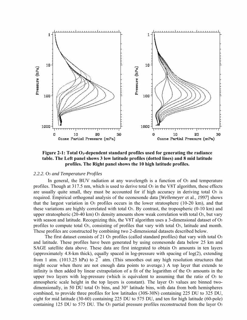
Figure 2-1: Total O3-dependent standard profiles used for generating the radiance table. The Left panel shows 3 low latitude profiles (dotted lines) and 8 mid latitude

profiles. The Right panel shows the 10 high latitude profiles.

2.2.2. O3 and Temperature Profiles In general, the BUV radiation at any wavelength is a function of O3 and temperature

profiles. Though at 317.5 nm, which is used to derive total O3 in the V8T algorithm, these effects are usually quite small, they must be accounted for if high accuracy in deriving total O3 is required. Empirical orthogonal analysis of the ozonesonde data [Wellemeyer et al., 1997] shows that the largest variation in O3 profiles occurs in the lower stratosphere (10-20 km), and that these variations are highly correlated with total O3. By contrast, the tropospheric (0-10 km) and upper stratospheric (20-40 km) O3 density amounts show weak correlation with total O3, but vary with season and latitude. Recognizing this, the V8T algorithm uses a 3-dimensional dataset of O3 profiles to compute total O3, consisting of profiles that vary with total O3, latitude and month. These profiles are constructed by combining two 2-dimensional datasets described below.

The first dataset consists of 21 O3 profiles (called standard profiles) that vary with total O3 and latitude. These profiles have been generated by using ozonesonde data below 25 km and SAGE satellite data above. These data are first integrated to obtain O3 amounts in ten layers (approximately 4.8-km thick), equally spaced in log-pressure with spacing of log(2), extending from 1 atm. (1013.25 hPa) to 2

-10

atm. (This smoothes out any high resolution structures that might occur when there are not enough data points to average.) A top layer that extends to infinity is then added by linear extrapolation of a fit of the logarithm of the O3 amounts in the upper two layers with log-pressure (which is equivalent to assuming that the ratio of O3 to atmospheric scale height in the top layers is constant). The layer O3 values are binned two-dimensionally, in 50 DU total O3 bins, and 30° latitude bins, with data from both hemispheres combined, to provide three profiles for low latitudes (30S-30N) containing 225 DU to 325 DU, eight for mid latitude (30-60) containing 225 DU to 575 DU, and ten for high latitude (60-pole) containing 125 DU to 575 DU. The O3 partial pressure profiles reconstructed from the layer O3

amounts are shown in Fig. 2-1. They capture the well-known features of the O3 vertical distribution, namely, that in a given latitude band the O3 peak and the O3 tropopause get lower as total O3 increases, and for a given total O3 the peak gets lower as one moves to higher latitude. Empirical orthogonal function analysis shows that the standard profiles capture the first two eigen-functions of the O3 profile covariance matrix well, and explain about 80% of the variance of the layer O3 amounts [Wellemeyer et al., 1997]. However, the scheme doesn’t capture the seasonal variation of O3 at altitudes where the O3 profile is not correlated with total O3 (the troposphere and altitudes above 25 km). Also, since a single US standard temperature profile is used in constructing the radiance tables, the effects of seasonal and latitudinal variation of temperature on O3 cross-sections are not accounted for.

The previous BUV algorithms had ignored these effects, since their absence did not increase the RMS error of a single measurement significantly and had virtually no impact on global O3 trend. This practice is consistent with that used by ground-based Dobson instruments, which also ignore seasonal and latitudinal variations in atmospheric temperature in retrieving total O3 from their measurements. However, with improving accuracy of the various O3 measuring systems, and with increasing emphasis on extracting weak tropospheric O3 signatures from total O3 measurements [Fishman et al., 1986; Ziemke et al., 1998] these small errors become more noticeable. We correct these errors in V8T by incorporating monthly and latitudinally varying O3 and temperature climatologies in the retrieval algorithm [based on the work described in McPeters, Logan, & Labow 2003].

The 3-dimensional profiles are constructed by combining these two datasets in such a way that in the part of the atmosphere where total O3 is a good predictor of O3 profile the 1st dataset prevails while in the rest of the atmosphere the 2nd data set prevails. This results in 1512 profiles, 12Xn profiles in each of the 18 latitude bins, where n is 3 in low latitudes (30S-30N), 8 in mid latitude (30°-60°), and 10 in high latitudes (60°-90°), containing the same total O3 as in the first dataset. These profiles are slightly different in the two hemispheres, primarily due to hemispherical asymmetry in the tropospheric O3. Since the errors in switching from the 21 profiles to the larger set are small, we have judged that it is sufficiently accurate to correct for them using Jacobians - defined as dlogI/dx, where I is the TOA (top of atmosphere) radiance, and x is the layer O3 amount in ~4.8 km [∆log(p)=log(2)] atmospheric layers. The Jacobian is calculated by the finite difference method for each entry in the basic radiance table. (The Jacobian can be provided in the output file so a user can readily calculate the impact of using an alternative O3 or temperature profile on the retrieved O3 without going through the full algorithm. This should be particularly useful for the assimilation of total O3 data using techniques based on 3-dimensional chemical and transport models.)

Figure 2-2 shows scatter plots comparing layer O3 amounts measured by the Hohen-peissenberg ozonesonde station with the 96 profile subset of the 3D profiles at that latitude. In layers 2 to 4, the correlations between the two are ~85%. Table 2-1 shows the variation reduction and residual standard deviation with this station and the SAGE satellite data at 50°N. The residual standard deviation in all layers is less than 10 DU. Similar results are obtained at other latitudes.

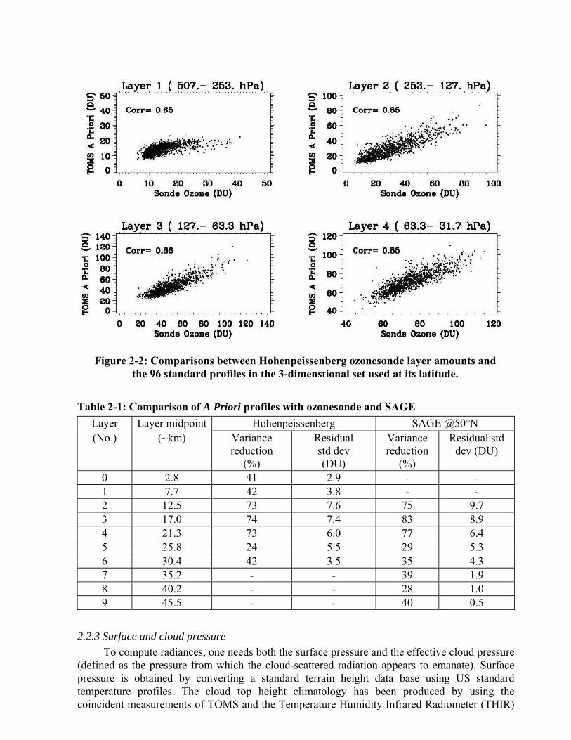
Figure 2-2: Comparisons between Hohenpeissenberg ozonesonde layer amounts and

the 96 standard profiles in the 3-dimenstional set used at its latitude. Table 2-1: Comparison of A Priori profiles with ozonesonde and SAGE

Layer Layer midpoint Hohenpeissenberg SAGE @50°N (No.) (~km) Variance

reduction (%)

Residual std dev (DU)

Variance reduction

(%)

Residual std dev (DU)

0 2.8 41 2.9 - - 1 7.7 42 3.8 - - 2 12.5 73 7.6 75 9.7 3 17.0 74 7.4 83 8.9 4 21.3 73 6.0 77 6.4 5 25.8 24 5.5 29 5.3 6 30.4 42 3.5 35 4.3 7 35.2 - - 39 1.9 8 40.2 - - 28 1.0 9 45.5 - - 40 0.5

2.2.3 Surface and cloud pressure To compute radiances, one needs both the surface pressure and the effective cloud pressure

(defined as the pressure from which the cloud-scattered radiation appears to emanate). Surface pressure is obtained by converting a standard terrain height data base using US standard temperature profiles. The cloud top height climatology has been produced by using the coincident measurements of TOMS and the Temperature Humidity Infrared Radiometer (THIR)

both onboard the Nimbus 7 Spacecraft. THIR cloud heights for clouds with high UV-reflectivity based on TOMS have been mapped onto a 2.5º latitude X 2.5º longitude grid for each month. These high reflectivity cloud heights are appropriate for the V8T cloud and surface reflectivity model described below in Section 2.2.4. The surfaces are also flagged as containing snow/ice by using a climatological database. There is no difficulty in substituting improved information on ground cover from current observations or forecasts.

2.2.4 Radiance Computation Using the output of TOMRAD, one calculates the TOA radiance, I, by using the following

formula:

I = I0 θ0,θ( )+ I1 θ0,θ( )cosφ + I2 θ0,θ( )cos2φ +RIR θ0,θ( )1− RSb( ) (2.1)

where, the first three terms constitute the purely atmospheric component of the radiance, unaffected by the surface. This component, which we will refer to as Ia, is a function of solar zenith angle θ0, satellite zenith angle θ, and φ, the relative azimuth angle between the plane containing the sun and local nadir at the viewing location and the plane containing the satellite and local nadir. The last term provides the surface contribution, where, the product R IR is the once-reflected radiance from a Lambertian surface of reflectivity R, and the factor (1-RSb)

-1

accounts for multiple reflections between the surface and the overlying atmosphere. Note that this factor can greatly enhance the effect of absorbers (e.g., tropospheric O3, O2-O2, UV-absorbing aerosols, and SO2) that may be present just above a bright surface. The tables are computed for ten solar zenith angles and six satellite zenith angles, which have been selected so that the interpolation errors in the computed radiances are typically smaller than 0.1% using a carefully constructed piecewise cubic interpolation scheme.

The forward model does not account for aerosols explicitly. This decision has been made deliberately since, as shown by Dave [1978], common types of aerosols (sea-salt, sulfates etc.) can be treated simply by increasing the apparent reflectivity of the surface, i.e., by increasing R in Eq. (2.1), to match the measured radiances at a weakly ozone-absorbing wavelength. This also avoids the need for knowing the true reflectivity of the surface. However, one must make a key assumption that the reflectivity thus derived is spectrally invariant over the range of wavelength of interest (310 nm to 330 nm). It is now known that UV-absorbing aerosols (smoke, mineral dust, volcanic ash) introduce a spurious spectral dependence in R, for they absorb the (strongly wavelength-dependent) Rayleigh-scattered radiation passing through them [Torres et al., 1998]. This absorption obviously varies with the height of the aerosols as well as on their microphysical properties; both of which are highly variable in space and time. Therefore, it is not possible to account for them explicitly in the forward model. In the next section we will discuss how we detect and correct for them in the inverse model.

The forward model treats a cloud as an opaque Lambertian surface. Transmission through and around clouds is accounted for by a partial cloud model, in which the TOA radiance I is written as:

I = Is Rs, ps( )1− fc( )+ Ic Rc, pc( ) fc (2.2)

where, Is represents radiance from the clear portion of the scene, containing a Lambertian surface of reflectivity Rs at pressure ps; and Ic similarly represents the cloudy portion, and fc is the cloud fraction. As shown in Fig. 2-3, the best agreement between the spectral dependence of TOA reflectance ( ρ = πI F cosθ0 ) observed by TOMS and that calculated by using Eq. (2.2) is

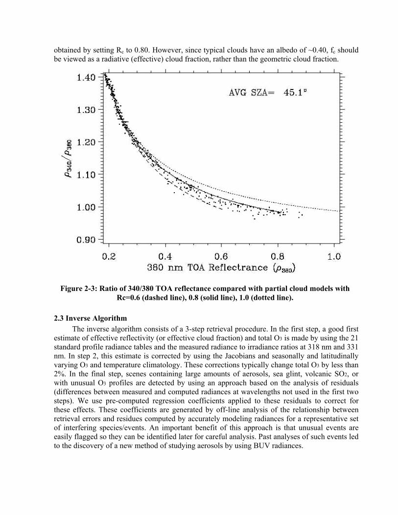
obtained by setting Rc to 0.80. However, since typical clouds have an albedo of ~0.40, fc should be viewed as a radiative (effective) cloud fraction, rather than the geometric cloud fraction.

Figure 2-3: Ratio of 340/380 TOA reflectance compared with partial cloud models with Rc=0.6 (dashed line), 0.8 (solid line), 1.0 (dotted line).

2.3 Inverse Algorithm The inverse algorithm consists of a 3-step retrieval procedure. In the first step, a good first

estimate of effective reflectivity (or effective cloud fraction) and total O3 is made by using the 21 standard profile radiance tables and the measured radiance to irradiance ratios at 318 nm and 331 nm. In step 2, this estimate is corrected by using the Jacobians and seasonally and latitudinally varying O3 and temperature climatology. These corrections typically change total O3 by less than 2%. In the final step, scenes containing large amounts of aerosols, sea glint, volcanic SO2, or with unusual O3 profiles are detected by using an approach based on the analysis of residuals (differences between measured and computed radiances at wavelengths not used in the first two steps). We use pre-computed regression coefficients applied to these residuals to correct for these effects. These coefficients are generated by off-line analysis of the relationship between retrieval errors and residues computed by accurately modeling radiances for a representative set of interfering species/events. An important benefit of this approach is that unusual events are easily flagged so they can be identified later for careful analysis. Past analyses of such events led to the discovery of a new method of studying aerosols by using BUV radiances.

2.3.1 Step 1: Initial total O3 estimation This step consists of the following sub-steps.

Step 1.1: By assuming a nominal total O3 amount, calculate the effective reflectivity of the scene by inverting Eq. (2.1). The inverse equation is:

R =Im − Ia( )

IR − Sb Im − Ia([ )] (2.3)

where, Im is the measured radiance at 331 nm, and Ia and IR are calculated using the climatological surface pressure (ps) appropriate for the scene. If 0.15<R<0.80, and the snow/ice and sea-glint flags are not set, compute effective cloud fraction fc by inverting Eq. (2.2), i.e.,

fc=(Im-Is)/(Ic-Is) (2.4) where Is and Ic are computed using Eq. (2.1) assuming Rs=0.15 and Rc=0.8. Note that the surface is assumed to have a reflectivity of 15%, even though the UV reflectivity of most surfaces (not covered with snow/ice) is between 2-8% [Herman & Celarier, 1997]. A larger value is used to account for haze, aerosols, and fair-weather cumulus clouds that are frequently present over the oceans at very low altitudes. We believe that treating them as part of the surface rather than as part of (a higher-level) cloud offers the best strategy to minimize errors. However, the method may produce small errors (1-2 DU) when cirrus clouds are present.

If R derived from Eq. (2.3) is greater than 0.80, we assume that the surface contribution to the radiance is zero. The (Lambertian-equivalent) cloud reflectivity is then derived using Eq. (2.3) assuming the surface is at pc. When the snow/ice flag is set, we currently assume that the cloud contribution to the radiances is negligible, and that R derived from Eq. (2.3) using ps represents the surface reflectivity. Step 1.2: Using R or fc and equations (2.1) and (2.2) compute the radiance as a function of total O3 amount (Ω) at 317.5 nm. Estimate O3 by a piecewise-linear fit on log(I) vs. Ω, i.e.,

Ω1 = Ωi + ln Im − ln I i( ) ∂ lnI∂Ω i,i+1

(2.4)

where, the measured radiance Im lies between Ii and Ii+1, computed using profiles with total O3 amounts Ωi and ΩI+1, respectively. Iterate steps 1.1 and 1.2 to correct for the total O3 dependence of the 331.2 nm wavelength. Convergence is achieved in one or two iterations.

At the termination of the iteration, one has the estimated O3 value Ω1, as well as the O3 profile (X1) which has been used to estimate it. This O3 profile is given by interpolation of the standard profiles, namely,

X1= Xi+(Xi+1-Xi)(Ω1-Ωi)/(Ωi+1-Ωi) (2.5)

Where Xi and Ωi are ozone profiles and total ozone amounts, respectively, for profile standard profile i. 2.3.2 Step 2: O3 and Temperature climatology correction In step 2, we adjust the solution total O3 to be consistent with a climatological O3 profile (X2) and a climatological temperature profile (T2). The Step 2 total O3, Ω2 is obtained as follows:

Ω2 = Ω1 +x2,l − x1,l[ ]

l∑ ∂ lnI

∂xl+ σ T2,l( )− σ T1,l( )[ ]∂ln I

∂σ l

∂ ln I∂Ω

(2.6)

where, l refers to the layer number, and σ(T) is the O3 absorption cross-section at temperature T. The Jacobian ∂ln I ∂σ is calculated from ∂ln I ∂x by using the chain rule for partial derivatives and that the radiances are functions of the products of x and σ, so

∂ ln I∂σ l

=∂ ln I∂xl

xl

σ l (2.7)

The O3 profile climatology used to provide (X2) is dependent on latitude and season as

well as total O3. A two step process was used to create the climatology in order to combine available information. First, the total O3 dependent standard profiles used to produce X1 (Equation 2.5) are combined with a climatology of seasonally and latitudinally varying O3 profiles that has no total O3 dependence. This procedure of merging the two climatologies has been carefully designed to account for the strengths and weaknesses of the two. We assume that the total O3 dependent standard profiles are most accurate in atmospheric layers where the layer O3 is highly correlated with total O3 (30 hPa- tropopause), while the seasonal climatology is better in all other layers. The merged climatology of profiles (X2) is constructed as follows:

X2=X1+ [Xc -Xs(Ωc)] (2.8)

where, Xc is the climatological profile (interpolated to the time and location of the measurement) and Xs is the standard profile (Fig. 2-1) interpolated to the same total O3 (Ωc) as contained in Xc. Note that, since Ωc and Ωs are the same, the procedure conserves total O3, i.e., Ω2=Ω1. It also retains X1 in those layers in which Xc and Xs are nearly the same. This occurs in those layers where total O3 is a good predictor of the O3 profile. In layers in which Xs doesn’t vary with total O3 (Fig. 2-1), X1 and Xs are the same, so X2 becomes equal to Xc.

This procedure works quite well except at high latitudes where the large dynamic range of total O3 amounts seems to thwart the use of Eq. (2.8) to determine profile shape characteristics for all total O3 amounts based on a mean profile. In these regions as a second step, we have used SBUV profile information to adjust the total O3 dependence of the merged climatology.

Comparison with sonde and satellite data shows that the X2 profile set explains a large portion of the variance of the O3 profiles seen at all altitudes, indicating that Eq. (2.8) provides a reliable method of generating a priori O3 profiles over the entire globe that vary correctly with season and total O3.

The temperature profile T2 corresponding to X2 is obtained simply by interpolation using a (month x latitude) climatology of temperature profiles obtained from NOAA/NCEP data. 2.3.3 Step 3: Correction of errors due to episodic events

Using R (or fc), which is assumed to be wavelength independent, Ω2, and the associated O3 and temperature profiles X2 and T2, it is straightforward to use the radiance and Jacobian tables to predict the radiance at each SBUV/2 wavelength. We call the percentage difference between the measured and predicted radiances the residuals. If the quantities that have been derived, and the assumptions made in deriving them are valid, the residuals should be zero, so a non-zero residue is an indicator of combined errors due to the forward model, the inverse model

and the instrument calibration. Experience with TOMS, supported by extensive simulation of various errors by using radiative transfer code, suggests that the analysis of spatial and temporal variability of the residual can yield many valuable clues to separate these various error sources. In many cases a simple correction procedure based on these residues can be developed. In the following, we provide examples of errors that can be detected and corrected this way.

Aerosols TOMS data show very clearly that the apparent reflectivity of the Earth’s surface derived

from Eq. (2.3) has a strong wavelength dependence in the presence of mineral dust and carbonaceous aerosols. Mie scattering calculations show that this is caused by the absorption of direct and Rayleigh-scattered radiation as it passes through the aerosol layer. Since this scattering increases with decreasing wavelength, the apparent reflectivity of the surface (obtained by neglecting the aerosol absorption) decreases with wavelength. When one uses only two wavelengths to derive O3, this absorption produces an effect that cannot be distinguished from O3 absorption, and hence one overestimates total O3. The V8T algorithm corrects for this effect by taking advantage of the fact that the effect on radiances of the R-λ dependence produced by aerosols can be readily observed by using two weakly-absorbing wavelengths that are separated in wavelength. For TOMS, we use wavelengths 331.2 and 360 nm. For SBUV/2, the photometer channel at 380 nm is used with the monochromator 331-nm channel.

When one uses the R derived from 331 nm to calculate a radiance at 380 nm, the R-λ dependence produces a residue at 380 nm. This residue is positive when absorbing aerosols are present. By Mie scattering calculation, using various types of absorbing and non-absorbing aerosols, Torres & Bhartia [1999] showed that for the TOMS V7 algorithm a simple linear relationship between the residues and the O3 error exists. Similar calculations using the TOMS V8T algorithm indicate that O3 is overestimated by ~2.5±0.5 DU when the 360-nm residue is 1%. The uncertainty represents variations in the estimated corrections due to aerosol type, their vertical distribution, and observational geometry. This means that in extreme cases, when the 360-nm residue reaches 10%, the maximum corrections are 25±5 DU. We estimate that the error in this aerosol correction is 1.5%.

Mie scattering calculations show that the non-absorbing aerosols can also produce residues, but for reasons that are more conventional. It is well known that the optical depth of aerosols consisting of small particles varies as λ

-A

, where A is called the Ångstrom coefficient and is typically close to 1. This produces a greater increase in BUV radiances (above the Rayleigh background) at shorter wavelengths than at longer wavelengths, thus producing O3 underestimation and a negative residue at 380 nm. However, compared to absorbing aerosols these effects are small. TOMS data indicate that 360-nm residues are rarely less than –2%. From Mie scattering calculation, the coefficient of correction comes out to be the same as for absorbing aerosols, i.e., -2.5 DU for -1% residue at 360 nm.

Since relatively large residues, not related to aerosols, are seen at large solar zenith angles in the TOMS data, the aerosol correction is applied only when the solar zenith angle is less than 60˚. TOMS data indicate that aerosol amounts are large enough to produce a 1% residue at 360 nm roughly 30% of the time, and most of these corrections are less than 5 DU. The larger SBUV/2 FOV increases the portion of data with aerosols present.

Sun-Glint The apparent reflectivity of the ocean in the BUV in the glint direction (roughly a cone of

±15˚ from the nadir for the SBUV/2) varies with wavelength due to variations in the direct to diffuse ratio of the radiation falling on the surface. The magnitude of the sea-glint, and hence the R-λ dependence it produces, decreases with increase in surface winds and by the presence of

aerosols and clouds which also decrease the direct to diffuse ratio. Radiative transfer calculations [Ahmad & Fraser, private communication] show that, though the cause of the R-λ dependence produced by sea-glint is quite different, its effect on O3 and residuals is similar to that for absorbing aerosols, and the same correction procedure also applies. As mentioned in section 1.2.6, the nadir-viewing geometry of the SBUV/2 and spacecraft orbits with equator crossing times more than an hour (15˚) from solar noon limit the occurrence of sea glint geometries.

However, there is one aspect of sea-glint that is different from absorbing aerosols- the fact that they can significantly increase the apparent brightness of the surface and are easily confused with clouds. Since sea-glint increases the absorption of radiation by O3 near the surface while clouds reduce the absorption, it is important to separate the two. The V8T distinguishes clouds from sea-glint using the fact that clouds do not produce residues. So, in situations where geometry indicates the potential for sea-glint, retrievals with 360 nm residue greater than 3.5% are flagged as effected by sea-glint in the TOMS V8T. Since the SBUV/2 instruments are nadir-viewing and lack a 360 nm channel. This flagging is not performed. O3 Profile

Strictly speaking, the BUV radiances at all wavelengths have some sensitivity to the vertical distribution of O3. Though the wavelengths used in the V8T algorithm to derive total O3 have been selected to minimize this effect, and the step 2 correction procedure described in section 2.3.2 has been designed to correct any residual systematic errors, there are situations when the profile errors become too large to be acceptable. These situations begin to occur when the O3 slant column density (SCD), Ω × (secθ+secθ0), exceeds 1500 DU. Studies of O3 in the polar regions require that the algorithm be able to derive reasonable total O3 values as close to the solar terminator as possible. At 80˚ soar zenith angle, the SCD can vary from less than 1000 DU to more than 4000 DU due to O3 variability, and simply discarding data with very large SCD would seriously bias the zonal means. Therefore, it is important to design the algorithm such that reasonable (5%, 1σ) total O3 values can be obtained for SCD of 5000 DU. From the error analysis of the TOMS algorithm [Wellemeyer et al., 1997], we have determined that errors at SCD>1500 DU typically occur when the assumed O3 profile near 10 hPa is significantly different from that assumed in step 2 (X2). The error occurs because the algorithm has been explicitly designed (by using the standard profiles shown in Fig. 2-1) to minimize errors near 100 hPa where most of the O3 variability takes place. This makes the algorithm sensitive to O3 profile variations away from the 100 hPa region. Fig. 2-4 shows how a 10% error in the assumed profile between 4 hPa and 32 hPa (representing roughly 1σ variation of O3 profile) affects the Step 2-derived total O3 as a function of SCD.

Fortunately, profile errors near 10 hPa can be detected by examining the residue at shorter BUV wavelengths which are more sensitive to O3 profile than the wavelengths used for deriving total O3. Fig. 2-5 shows how the 312.5 nm residue responds to the profile error assumed for Fig. 2-4. More detailed analysis of this error using a set of O3 profiles derived from high latitude ozonesondes indicates that a simple correction factor of 3.5 DU for 1% residue at 312.5 nm provides adequate correction to obtain reliable total O3 values (2%, 1σ) at SCDs of up to 3000 DU. However, the correction procedure becomes increasingly unreliable as the SCD exceeds 3000 DU.

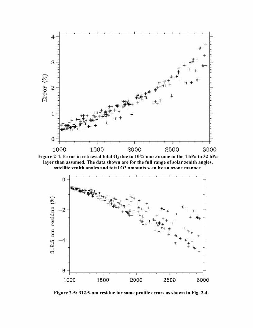
Figure 2-4: Error in retrieved total O3 due to 10% more ozone in the 4 hPa to 32 hPa layer than assumed. The data shown are for the full range of solar zenith angles,

satellite zenith angles and total O3 amounts seen by an ozone mapper.

Figure 2-5: 312.5-nm residue for same profile errors as shown in Fig. 2-4.

For SCD > 3000 DU, TOMS uses the 360-nm channel to derive surface reflectivity, so that the 331-nm residue, which is fairly sensitive to total O3 at these very high path lengths but insensitive to profile shape effects, can be used to identify error in the total O3 derived using 317.5 nm. The residue based correction to the derived O3 then is the product of the 331-nm residue and the total O3 sensitivity at 331 nm, ∂lnI/∂Ω. Sulfur dioxide (SO2)

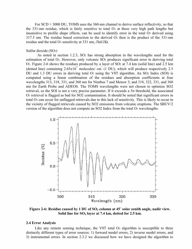
As noted in section 1.2.3, SO2 has strong absorption in the wavelengths used for the estimation of total O3. However, only volcanic SO2 produces significant error in deriving total O3. Figure 2-6 shows the residues produced by a layer of SO2 at 7.4 km (solid line) and 2.5 km (dotted line) containing 2.65x10

16

molecules/ cm2

(1 DU), which will produce respectively 2.5 DU and 1.3 DU errors in deriving total O3 using the V8T algorithm. An SO2 Index (SOI) is computed using a linear combination of the residues and absorption coefficients at four wavelengths 313, 318, 331, and 360 nm for Nimbus 7 and Meteor 3; and 318, 322, 331, and 360 nm for Earth Probe and ADEOS. The TOMS wavelengths were not chosen to optimize SO2 retrieval, so the SOI is not a very precise parameter. If it exceeds a 5σ threshold, the associated O3 retrieval is flagged as bad for SO2 contamination. It should be noted that significant errors in total O3 can occur for unflagged retrievals due to this lack of sensitivity. This is likely to occur in the vicinity of flagged retrievals caused by SO2 emissions from volcanic eruptions. The SBUV/2 version of the algorithm does not compute an SO2 Index from the total O3 wavelengths.

Figure 2-6: Residue caused by 1 DU of SO2 column at 45˚ solar zenith angle, nadir view. Solid line for SO2 layer at 7.4 km, dotted for 2.5 km.

2.4 Error Analysis Like any remote sensing technique, the V8T total O3 algorithm is susceptible to three

distinctly different types of error sources: 1) forward model errors, 2) inverse model errors, and 3) instrumental errors. In section 2.3.2 we discussed how we have designed the algorithm to

minimize the impact of the first two of these errors by carefully constructing the O3 and temperature profiles to remove any latitude and seasonally dependent biases from the data, and in section 2.3.3 we discussed how we use the residues to detect and correct errors that are localized in space and time. However, there are some errors that cannot be corrected by either of these methods. In this section we highlight these remaining errors. In addition, we discuss the sensitivity of the algorithm to instrumental errors. 2.4.1 Forward Model Errors

The forward model errors include errors that occur in the computation of radiances. Since even the best radiative transfer models can only approximate the complex scattering and absorption processes of the real atmosphere, one inevitably has errors. Since the retrieval algorithm essentially uses the difference between the measured and calculated radiances to derive O3, errors in forward model calculations are just as important, if not more important (given that they are systematic), as errors in measured radiance. However, it is important to note that the algorithm uses a pair of wavelengths to derive O3. Since these wavelengths are only 13 nm apart, relatively large errors in computing absolute radiances may not have much impact, while even small errors in computing the ratio of radiances become quite important. Following is a brief summary of key forward model errors.

Radiative Transfer Code The TOMRAD radiative transfer code, the work-horse of the V8T algorithm, assumes that

the atmosphere contains only molecular scatterers and absorbers bounded by opaque Lambertian surfaces. Radiation amounts from these surfaces are linearly mixed to simulate the effect of clouds. Clearly, this scheme is an overly simplified treatment of many complex processes that occur in a real atmosphere, including Mie scattering by clouds and aerosols, scattering by non-spherical dust particles, and reflection by non-Lambertian surfaces. However, as discussed in the previous section, the ability of this code to simulate the ratio of radiances at weakly-absorbing wavelengths can be tested using TOMS data. These tests show that the prediction of forward model works quite well over a very large range of conditions, with three key exceptions, two of which we have already noted: sea-glint and UV-absorbing aerosols. The third case usually occurs at large solar zenith angles in the presence of snow/ice, where the forward model underestimates the ratio of 340-nm/380-nm radiances by several percent. If this anomaly is caused by the presence of clouds over bright surfaces, as is strongly suspected, its impact on derived O3 would be small, since multiple scattering between the surface and clouds reduces the shielding effect of clouds.

Analysis of the ratio of 340-nm and 380-nm radiances, however, leaves out the possible effect of clouds, aerosols and surfaces in changing the absorption of radiation by O3. To understand these effects, we use a more realistic radiative transfer model in which we assume that clouds are homogeneous and plane-parallel layer of Mie scatterers. We calculate the effect of clouds on the BUV radiances using the Gauss-Seidel vector code [Herman & Browning, 1965] using Deirmendjian’s [Deirmendjian, 1969] C1 cloud model. By varying the cloud optical depth in this model one can produce a curve similar to that shown in Fig. 2-2. Comparison with TOMS data shows similar good agreement, which leads us to believe that this model is a reasonable way to model cloud effects in UV, with the advantage that one can account for surface-cloud interactions that the operational model ignores. However, detailed comparison of the results from the two models indicates that despite their drastically different characterization of clouds, the total O3 derived from these models are essentially the same (within ±1%), provided one uses the correct effective pressure of the clouds. (The effective pressure of the cloud is usually greater, i.e., the clouds scattering emanates from lower altitude, than the cloud

top pressure, depending upon the optical and physical thickness of the clouds, surface albedo and observation geometry. It is expected that UV or visible cloud algorithms would provide a more accurate value of this pressure than infrared algorithms, which sense the black-body temperature of cloud-tops, for all but very thin clouds, such as cirrus.)

This error analysis does not apply to clouds and aerosols in the stratosphere, which can significantly alter the absorption of the BUV radiation by stratospheric O3, producing relatively large errors. It has been shown [Torres et al., 1992; Bhartia et al., 1993] that at high solar zenith angles (θo>80˚) stratospheric clouds (e.g., PSCs) and aerosols may cause the total O3 to be significantly underestimated, provided they are sufficiently optically thick (τ>0.1) and are close to the O3 density peak. This is because the photons scattered in the stratosphere do not sense the entire O3 column. However, at lower solar zenith angles, the error can be either positive or negative and may vary in a complicated way with observation geometry. Though it is known that optically thick Type III PSCs containing water ice do form due to adiabatic ascent of air as it passes over orographic features (lee waves), sometimes creating localized O3 depletion called a “mini-hole”, it is not known if the optical depth of these clouds is large enough, or if they are high enough, to produce the errors postulated by Torres et al. [1998]. However, the effects of high altitude stratospheric aerosols that form after volcanic eruptions are well understood [Torres et al., 1995]. Bhartia et al. [1993] estimate that the stratospheric aerosols created few months after the 1991 eruption of Mt. Pinatubo volcano in the Philippines introduced errors in the BUV total O3 retrieval of +6 to -10%, depending on solar zenith angle, though these errors subsided quickly after 6 months as the altitude of the aerosols dropped.

To summarize, under normal circumstances for SBUV/2 and TOMS, the radiative transfer modeling errors would contribute approximately 1.5% (1σ) error in the computation of O3. However, in the presence of Type III PSCs, and for several months after high altitude volcanic eruptions, the errors may be an order of magnitude larger.

Spectroscopic Constants Several groups have made measurements of O3 absorption cross-sections recently. Based

on evaluation of Bass & Paur [1984] measurements by Chance [private communication], it is estimated that at the wavelengths used to derive total O3 (317.5 nm) Bass and Paur measurements are probably accurate to better than 2%. We have used the Bass and Paur measurements shortward of 340 nm, and FTS Measurements from University of Bremen [S. Voight, private communication, 2001]. Uncertainty in molecular scattering cross-sections are generally considered small (<1%), and in any case the errors are not likely to vary significantly with wavelength to affect derived total O3. Some non-physical values for the temperature dependence of the O3 cross-sections have been found in the Bass and Paur data sets and alternative sources are under evaluation.

2.4.2 Inverse Model Errors In remote sensing problems, the inverse model errors are caused by the fact that the

inversions of radiances into geophysical parameters require a priori information. This is true of even the simplest type of remote sensing, e.g., measurement of total O3 using direct solar radiation, as employed by ground-based Dobson and Brewer instruments. The inversion algorithms for these instruments require some knowledge of how the O3 is distributed vertically in the atmosphere in order to correct for the effects of atmospheric temperature on O3 absorption cross-section, and for the effect of Earth’s sphericity on the airmass factor. Errors in a priori, therefore, inevitably introduce retrieval errors; though for Dobson and Brewer algorithms they are usually quite small (<1%). The following is a summary of these errors for the V8T algorithm.

O3 Profile As discussed in section 2.3, the V8T algorithm uses an elaborate scheme to minimize

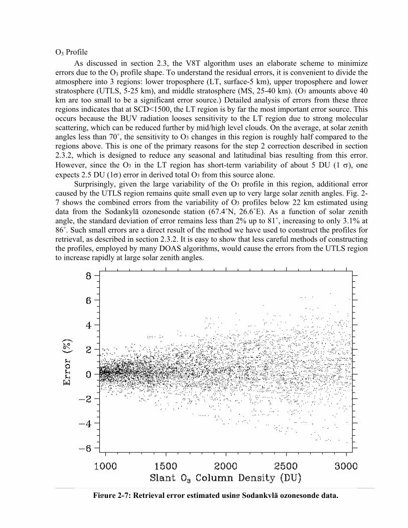
errors due to the O3 profile shape. To understand the residual errors, it is convenient to divide the atmosphere into 3 regions: lower troposphere (LT, surface-5 km), upper troposphere and lower stratosphere (UTLS, 5-25 km), and middle stratosphere (MS, 25-40 km). (O3 amounts above 40 km are too small to be a significant error source.) Detailed analysis of errors from these three regions indicates that at SCD<1500, the LT region is by far the most important error source. This occurs because the BUV radiation looses sensitivity to the LT region due to strong molecular scattering, which can be reduced further by mid/high level clouds. On the average, at solar zenith angles less than 70˚, the sensitivity to O3 changes in this region is roughly half compared to the regions above. This is one of the primary reasons for the step 2 correction described in section 2.3.2, which is designed to reduce any seasonal and latitudinal bias resulting from this error. However, since the O3 in the LT region has short-term variability of about 5 DU (1 σ), one expects 2.5 DU (1σ) error in derived total O3 from this source alone.

Surprisingly, given the large variability of the O3 profile in this region, additional error caused by the UTLS region remains quite small even up to very large solar zenith angles. Fig. 2-7 shows the combined errors from the variability of O3 profiles below 22 km estimated using data from the Sodankylä ozonesonde station (67.4˚N, 26.6˚E). As a function of solar zenith angle, the standard deviation of error remains less than 2% up to 81˚, increasing to only 3.1% at 86˚. Such small errors are a direct result of the method we have used to construct the profiles for retrieval, as described in section 2.3.2. It is easy to show that less careful methods of constructing the profiles, employed by many DOAS algorithms, would cause the errors from the UTLS region to increase rapidly at large solar zenith angles.

Figure 2-7: Retrieval error estimated using Sodankylä ozonesonde data.

At SCD>1500 DU, the profile effect of the MS region starts to become important. However, error analysis using high latitude O3 profiles obtained from satellites indicate that the step 3 profile correction (described in section 2.3.3) works quite well. The residual errors are estimated to be ~1.5% (1σ), increasing to 5% at SCD of 5000 DU. If the maximum-likelihood-estimation procedure is employed, then these errors can be reduced further. Total RMS errors due to variations in the O3 profile are: ~1.5% up to 70˚ solar zenith, ~3% at 82˚ and ~5% at 85˚.

Temperature Profile Step 2 of the algorithm corrects for seasonal and latitudinal variation of the atmospheric

temperature. Residual errors are less than 0.5% (1σ). Though the errors can become larger in the polar regions, the O3 profile errors remain the dominant error source at all latitudes. Therefore, at present, we do not see any need to bring in daily temperature maps to improve our total O3 estimates.

2.4.3 Instrumental Errors Instrumental errors include systematic errors due to pre-launch errors in instrument

calibration (spectral and radiometric), calibration drift after launch, and random noise. Since we do not yet know how large these errors are likely to be, we provide sensitivity to various errors in the following.

Spectral Calibration The 317.5-nm wavelength channel is located on a plateau in the O3 absorption cross-

section; hence it is not particularly sensitive to wavelength errors: a 0.01-nm error in wavelength produces 0.1% error in O3. This is roughly the uncertainty in the SBUV/2 wavelength scale calibration.

Radiometric Calibration Unlike DOAS algorithms, the V8T algorithm is quite sensitive to radiometric calibration

errors. A 1% calibration error, independent of wavelength between 317.5 nm and 331.2 nm, introduces a 0-2 DU O3 error depending on brightness of the scene. (Larger errors occur for darker scenes.) A 1% relative calibration error between the two wavelengths introduces ~4-6 DU error depending on slant column O3 amount. (The smallest errors occur at SCD of ~1000 DU.) Over the years, several strategies have been developed to detect the calibration errors by the analysis of residues. We estimate that the radiometric calibration of an individual SBUV/2 total O3 or reflectivity is accurate to 1%, and may contain drifts of 1%/decade or less after retrospective characterization. Operational variations for total O3 channels may reach 2%.

Instrument Noise A 1% instrument noise at each of the two wavelengths used for total O3 retrieval would

lead to 6 DU to 9 DU noise in total O3. The noise of the SBUV/2 instrument in total O3 and reflectivity channels is 2 to 4 times better than this, so its effect will be well below the systematic errors and therefore of little significance.

2.4.4 Error Summary All the important error sources we have discussed above are systematic, i.e., the errors are

repeatable given the same geophysical conditions and viewing geometry. However, most errors vary in a pseudo-random manner with space and time, so they tend to average out when data are averaged or smoothed. The best way to characterize these errors is as follows: the errors at any given location would have a roughly Gaussian probability distribution with standard deviation of

about 2% at solar zenith angles less than 70˚, increasing to 5% at 85˚, with a non-zero mean. The means themselves will have a roughly Gaussian distribution with standard deviation of about 1% with non-zero mean of ±2% (due to error in O3 absorption cross-section). Conservatively, one should assume that the latter error distribution is not affected by the amount of smoothing, i.e., it remains the same whether one looks at monthly mean at any given location, daily zonal mean, monthly zonal mean, or even yearly mean 2.5 References Ahmad, Z. & P.K. Bhartia, “Effect of Molecular Anisotropy on the Backscattered UV

Radiance,” Appl. Opt., 34, 8309-8314, 1995. Bass, A.M. & R.J. Paur, “The ultraviolet cross-section of ozone: I The measurements,” in

Atmospheric Ozone, edited by C.S. Zerefos and A, Ghazi, 606-610, D. Reidel, Norwood, Mass., 1984.

Bates, D. R., “Rayleigh scattering by air,” Planet. Space Sci., 32, 785-790, 1984. Bhartia, P.K., et al., “Effect of Mount Pinatubo Aerosols on Total Ozone Measurements From

Backscatter Ultraviolet (BUV) Experiments,” J. Geophys. Res., 98, 18547-18554, 1993. Brion, J., et al., “High-resolution laboratory absorption 23 cross section of O3. Temperature

effect,” Chem. Phys. Lett., 213 (5-6), 610-512, 1993. Caudill, T.R., et al., “Evaluation of the pseudo-spherical approximation for backscattered

ultraviolet radiances and ozone retrieval,” J. Geophys. Res., 102, 3881-3890, 1997. Deirmendjian, D., Electromagnetic scattering on spherical polydispersions, Elsevier, 290, 1969. Greenblatt, G.D., et al., “Absorption Measurements of Oxygen Between 330 and 1140 nm,” J.

Geophys. Res., 95, 18,57718,582, 1990. Dave, J. V., “Meaning of successive iteration of the auxiliary equation of radiative transfer,”

Astrophys. J., 140, 1292-1303, 1964. Dave, J.V. & C.L. Mateer, “A preliminary study on the possibility of estimating total

atmospheric ozone from satellite measurements,” J. Atmos. Sci., 24, 414-427, 1967. Dave, J.V., “Effect of Aerosols on the estimation of total ozone in an atmospheric column from

the measurements of its ultraviolet radiance,” J. Atmos. Sci., 35, 899-911, 1978. Eck, T.F., et al., “Reflectivity of the Earth's Surface and Clouds in Ultraviolet from Satellite

Observations,” J. Geophys. Res., 92, 4287, 1987. Fishman, J., et al., “Use of satellite data to study tropospheric ozone in the tropics,” J. Geophys.

Res., 91, 14,451-14,465, 1986. Herman, B.M., & S.R. Browning, “A numerical solution to the equation of radiative transfer,” J.

Atmos. Sci., 22, 559-566, 1965. Herman, J.R., & E.A. Celarier, “Earth surface reflectivity climatology at 340-380 nm from

TOMS data,” J. Geophys. Res., 102, 28003-28011, 1997. Joiner, J., et al., “Rotational-Raman Scattering (Ring Effect) in Satellite Backscatter Ultraviolet

Measurements,” Appl. Opt., 34, 4513-4525, 1995. Joiner, J. & P.K. Bhartia, “The Determination of Cloud Pressures from Rotational-Raman

Scattering in Satellite Backscatter Ultraviolet Measurements,” J. Geophys. Res., 100, 23019-23026, 1995.

Joiner, J. & P.K. Bhartia, “Accurate determination of total ozone using SBUV continuous spectral scan measurements,” J. Geophys. Res., 102, 12,957-12,970, 1997.

Klenk, K.F., et al., “Total ozone determination from the Backscattered Ultraviolet (BUV) experiment,” J. Appl. Meteorol., 21, 1672-1684, 1982.

Mateer, C.L., D.F. Heath, & A.J. Krueger, “Estimation of total ozone from satellite measurements of backscattered ultraviolet Earth radiance,” J. Atmos. Sci., 28, 1307-1311, 1971.

McPeters, R.D. et al., Nimbus-7 Total Ozone Mapping Spectrometer (TOMS) Data Products User's Guide, NASA Reference Publication 1384, 1996.

McPeters, R.D., J.A. Logan, & G.J. Labow, “Ozone Climatological Profiles for Version 8 TOMS and SBUV Retrievals.” A21D-0998, AGU Fall 2003.

Torres, O., Z. Ahmad & J.R. Herman, “Optical effects of polar stratospheric clouds on the retrieval of TOMS total ozone,” J. Geophys. Res., 97, 13015-13024, 1992.

Torres, O., et al., “Properties of Mt. Pinatubo Aerosols as Derived from Nimbus-7 TOMS Measurements,” J. Geophys. Res., 100, pp. 14,043-14,056, 1995.

Torres, O., et al., “Derivation of aerosol properties from satellite measurements of backscattered ultraviolet radiation: Theoretical basis,” J. Geophys. Res., 103, 17,099-17,110, 1998.

Torres, O. & P.K. Bhartia, “Impact of tropospheric aerosol absorption on ozone retrieval from backscattered ultraviolet measurements,” J. Geophys. Res., 104, 21569-21,577, 1999.

Voigt, S., et al.," The temperature dependence (203293 K) of the absorption cross sections of O3 in the 230-850 nm region measured by Fourier-Transform spectroscopy,“ J. Photochem. Photobiol. A, 143, 1-9, 2001.

Wellemeyer, C.G., et al., “A correction for total ozone mapping spectrometer profile shape errors at high latitude,” J. Geophys. Res., 102, 9029-9038, 1997.

Ziemke, J. R., S. Chandra & P.K. Bhartia, “Two New Methods of Deriving Tropospheric Column Ozone from TOMS Measurements: The Assimilated UARS MLS/HALOE and Convective Cloud Differential Technique,” J. Geophys. Res., 103, 22,115-22,127, 1998.

Chapter 3: Version 8 Vertical Profile O3 Algorithm 3.1 Background and Overview

The Version 8 O3 profile algorithm (V8P) is the latest in a series of BUV (backscattered ultraviolet) vertical profile O3 algorithms that have been developed for the SBUV and follow on SBUV/2 instruments. This chapter describes the basis for the V8P implementation with emphasis on the changes from the Version 6 O3 profile algorithm (V6A) it is replacing. The V6A is described in Bhartia et al. [1996] and in the OMPS Nadir Profile ATBD [Ball, 2002]. Both the V6A and V8P use optimal estimation to generate maximum likelihood retrievals. See Rodgers, [1976] and Rodgers, [1990] for theoretical analysis of the properties of this class of retrievals, and Meijer et al. [2006] for applications to O3 profile estimation. This chapter also makes frequent references to the two previous chapters’ descriptions of the physical basis of the measurements and the modeling techniques that are shared by the V8T and the V8P.

The Version 8 vertical profile O3 algorithm (V8P) is the first new SBUV/2 algorithm since the Version 6 (V6A) in 1990. The V8P uses a new set of profiles for the a priori information leading to better estimates in the troposphere (where SBUV/2 lacks retrieval information) and to simplified comparisons of SBUV/2 results to other measurement systems (in particular, the Umkehr ground-based O3 profile retrievals which now use the same set). The V8P has improved total O3 retrievals from improved multiple scattering and cloud and reflectivity modeling. Some errors present in the V6A will be reduced. These include a correction for 2% errors from previously ignoring the gravity gradient with height and elimination of 0.5% errors from low fidelity bandpass modeling. The V8P is also designed to allow the use of more accurate external and climatological data, to adjust for changes in wavelength selection, and to incorporate several ad hoc V6A improvements directly. Finally, the V8A is designed for expansion to perform retrievals for hyperspectral instruments, such as OMI, GOME and the Nadir Profiler in OMPS. Some components of the initial V8P implementation were optimized for trend detection. These are modified for use in operations but the algorithm has the flexibility to make these changes.

The Solar Backscatter Ultraviolet instruments, SBUV on Nimbus 7 and SBUV/2s on NOAA-9, -11, -14, -16 and -17 -18, are nadir-viewing instruments that infer total column O3 and the O3 vertical profile by measuring sunlight scattered from the atmosphere in the ultraviolet spectrum. Heath et al. [1975] describes the SBUV flown on Nimbus-7. Frederick et al. [1986], and Hilsenrath et al. [1995] describe the follow-on SBUV/2 instruments flown on the NOAA series of spacecraft.

The instruments are all of similar design; nadir-viewing double-grating monochromators of the Ebert-Fastie type. The instruments step through 12 wavelengths in sequence over 24 seconds, while viewing the Earth in the fixed nadir direction with an instantaneous field of view (IFOV) on the ground of approximately 180 km by 180 km. To account for the change in the scene-reflectivity due to the motion of the satellite during the course of a scan, a separate co-aligned filter photometer (centered at 343 nm on SBUV; 380 nm on SBUV/2) makes 12 measurements concurrent with the 12 monochromator measurements. Each sequence of measurements ends with an 8 second retrace, producing a complete set of measurements every 32 seconds on the daylight portions of an orbit.

The instruments are flown in polar orbits to obtain global coverage. Since the SBUV O3 measurements rely on backscattered solar radiation, data are only taken on the dayside of each orbit. There are about 14 orbits per day with 26° of longitudinal separation at the equator. Unfortunately, the early NOAA polar orbiting satellites are not sun-synchronous. For example, the NOAA-11 equator crossing times drifted from 1:30 pm (measurements at 30° solar zenith angle or so at the equator) at the beginning of 1989 to 5:00 pm by the end of 1995 (measurements at 70° solar zenith angle). As the orbit drifts, the terminator crossing location moves to lower latitudes and coverage decreases.

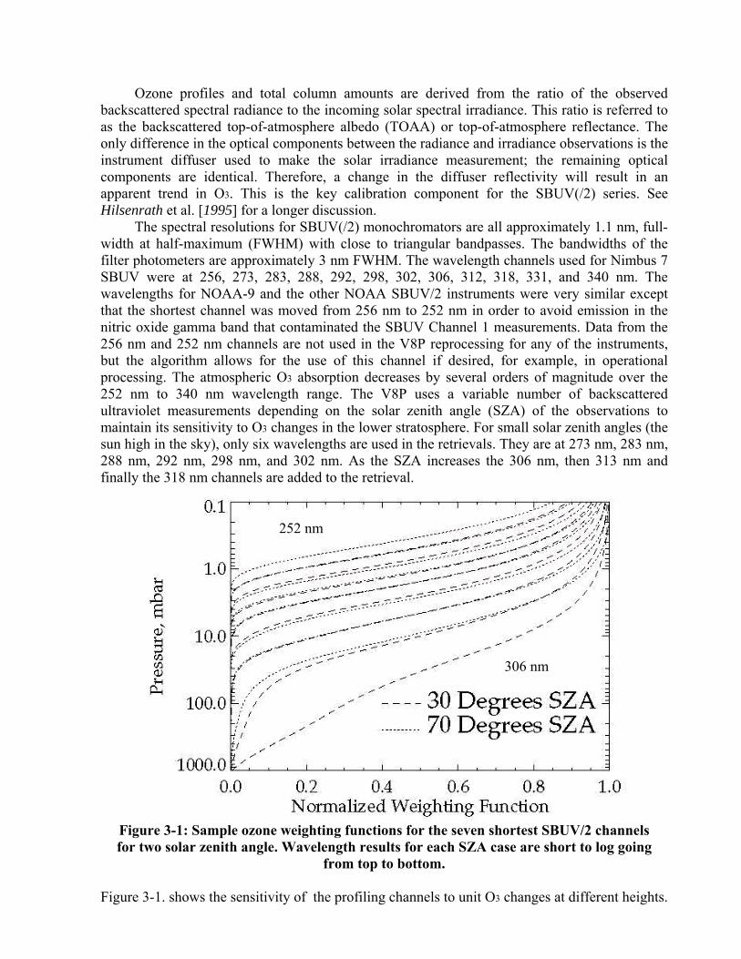
Ozone profiles and total column amounts are derived from the ratio of the observed backscattered spectral radiance to the incoming solar spectral irradiance. This ratio is referred to as the backscattered top-of-atmosphere albedo (TOAA) or top-of-atmosphere reflectance. The only difference in the optical components between the radiance and irradiance observations is the instrument diffuser used to make the solar irradiance measurement; the remaining optical components are identical. Therefore, a change in the diffuser reflectivity will result in an apparent trend in O3. This is the key calibration component for the SBUV(/2) series. See Hilsenrath et al. [1995] for a longer discussion.

The spectral resolutions for SBUV(/2) monochromators are all approximately 1.1 nm, full-width at half-maximum (FWHM) with close to triangular bandpasses. The bandwidths of the filter photometers are approximately 3 nm FWHM. The wavelength channels used for Nimbus 7 SBUV were at 256, 273, 283, 288, 292, 298, 302, 306, 312, 318, 331, and 340 nm. The wavelengths for NOAA-9 and the other NOAA SBUV/2 instruments were very similar except that the shortest channel was moved from 256 nm to 252 nm in order to avoid emission in the nitric oxide gamma band that contaminated the SBUV Channel 1 measurements. Data from the 256 nm and 252 nm channels are not used in the V8P reprocessing for any of the instruments, but the algorithm allows for the use of this channel if desired, for example, in operational processing. The atmospheric O3 absorption decreases by several orders of magnitude over the 252 nm to 340 nm wavelength range. The V8P uses a variable number of backscattered ultraviolet measurements depending on the solar zenith angle (SZA) of the observations to maintain its sensitivity to O3 changes in the lower stratosphere. For small solar zenith angles (the sun high in the sky), only six wavelengths are used in the retrievals. They are at 273 nm, 283 nm, 288 nm, 292 nm, 298 nm, and 302 nm. As the SZA increases the 306 nm, then 313 nm and finally the 318 nm channels are added to the retrieval.

252 nm

306 nm

Figure 3-1: Sample ozone weighting functions for the seven shortest SBUV/2 channels for two solar zenith angle. Wavelength results for each SZA case are short to log going

from top to bottom. Figure 3-1. shows the sensitivity of the profiling channels to unit O3 changes at different heights.

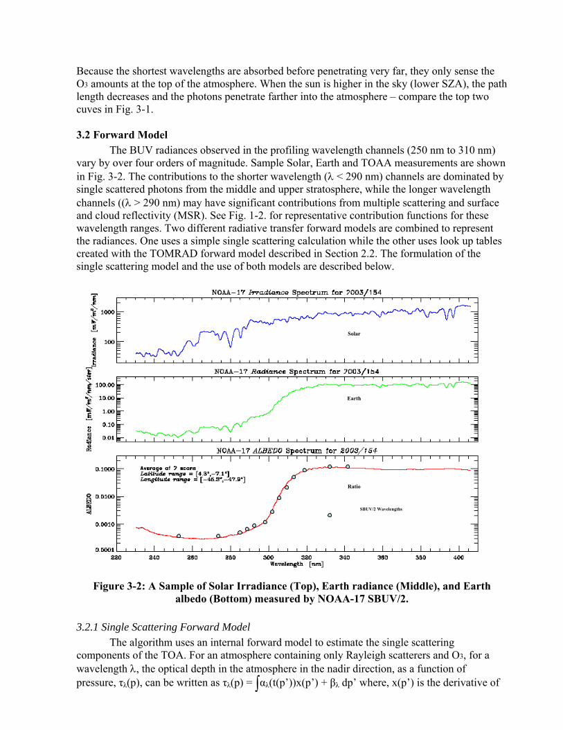
Because the shortest wavelengths are absorbed before penetrating very far, they only sense the O3 amounts at the top of the atmosphere. When the sun is higher in the sky (lower SZA), the path length decreases and the photons penetrate farther into the atmosphere – compare the top two cuves in Fig. 3-1. 3.2 Forward Model

The BUV radiances observed in the profiling wavelength channels (250 nm to 310 nm) vary by over four orders of magnitude. Sample Solar, Earth and TOAA measurements are shown in Fig. 3-2. The contributions to the shorter wavelength (λ < 290 nm) channels are dominated by single scattered photons from the middle and upper stratosphere, while the longer wavelength channels ((λ > 290 nm) may have significant contributions from multiple scattering and surface and cloud reflectivity (MSR). See Fig. 1-2. for representative contribution functions for these wavelength ranges. Two different radiative transfer forward models are combined to represent the radiances. One uses a simple single scattering calculation while the other uses look up tables created with the TOMRAD forward model described in Section 2.2. The formulation of the single scattering model and the use of both models are described below.

SBUV/2 Wavelengths

Solar

Earth

Ratio

Figure 3-2: A Sample of Solar Irradiance (Top), Earth radiance (Middle), and Earth

albedo (Bottom) measured by NOAA-17 SBUV/2. 3.2.1 Single Scattering Forward Model

The algorithm uses an internal forward model to estimate the single scattering components of the TOA. For an atmosphere containing only Rayleigh scatterers and O3, for a wavelength λ, the optical depth in the atmosphere in the nadir direction, as a function of pressure, τλ(p), can be written as τλ(p) = ∫αλ(t(p’))x(p’) + βλ dp’ where, x(p’) is the derivative of

the column O3 amount above a pressure p’ [x(p) = dX(p)/dp where X(p) is the partial column of ozone from the top of the atmosphere down to pressure p], αλ(t) is the O3 absorption coefficient at temperature t, and βλ is the Rayleigh scattering coefficient at a wavelength λ.

At wavelengths below 290 nm, little solar radiation penetrates below 30 km, permitting surface, cloud, and aerosol effects to be ignored. Because radiation is scattered from a region of the atmosphere which is optically thin for scattering, multiple scattering effects may also be ignored. For such cases, the backscattered radiance intensity in Eq. (2.1) can be explicitly written to a high degree of accuracy as

Rλ = (1/4π)Fλβλ P(cosθ0)∫exp[−∫s(p’)(αλ(t(p’))x( p’) +βλ )dp’] dp (3.1)

Where θ0 is the solar zenith angle, s is the slant path factor (air mass factor), P is the Rayleigh phase function, Fλ is the solar flux, and p is pressure. The outer integral limits are the surface to the top of the atmosphere. The inner integral limits are pressure p to the top of the atmosphere. This expression for Rλ is commonly described as the single scattering radiance. The Rayleigh phase function, P(cosθ0), assuming a depolarization factor of 0.035 (Bates, 1984), can be written as

P(cos θ0)= 0.7619 (1+ 0.937cos2 θ0). (3.2)

The slant path (air mass), s, for the SBUV/2 nadir viewing geometry, can be approximated by 1+sec(θ0) at low solar zenith angles (<60°), or by the Chapman (1931) function at moderate solar zenith angles (<80°). For solar zenith angles greater than 80°, s must be treated as a function of p, calculated by ray-tracing. The slant pass must also be modified to account for the increase in neutral atmosphere as a function of pressure increments with increasing height, that is, the gravity gradient. This increases the scatters by a factor of [1+H(p)/Re]2 where Re is the radius of the Earth at a surface at 1 atmosphere and H(p) is the physical height the layer at pressure p is above this surface. We will work with the top of atmosphere albedos (TOAA) I=R/F. The algorithm computes the single scattered albedos and the corresponding Jacobians of partial derivatives with respect to layer O3 amounts for given SBUV/2 channels by using a double discretization of Eq. (3.1) in atmospheric pressure and wavelength bandpass. The discretization in pressures represents the atmosphere by using 81 pressure layers with constant logarithmic spacing. Approximation of the atmosphere by using the pressure layers transforms the integral in Eq. 3.1 into a discrete sum with x(p) transformed into a corresponding discrete set of O3 layer amounts, and t(p) into a discrete set of mean layer temperature values. The partial derivatives of I with respect to O3 layer amounts can be efficiently computed by multiplying the component results for I by the appropriate –sα values and computing the appropriate sums. The second discretization concerns the representation of the wavelength channels 1.1-nm bandpasses. These are modeled by using a discrete set of 21 wavelengths spaced at 0.1 nm intervals around each bandpass center, multiplying the calculated Iλ for each wavelength by the relative bandpass contribution, and summing to provide the estimate of the full channel. Results using finer spacing and additional weighting to model solar variations produced small additional improvements. 3.2.2 Multiple Scattering Forward Model

The multiple-scattering forward model used in the V8P is the same radiative transfer forward model described in Section 2.2, namely, TOMRAD. Again it is used to create look-up

tables of radiances and Jacobians. In this case, the look-up tables give the relative changes between the MSR results and the single scattering results. That is, the tables give the ratio of full multiple scattering and reflectivity simulations and partial derivatives to corresponding single scattering ones. This means that they give the values to transform single scattering albedos or Jacobians computed by the internal forward model into full multiple scattering and reflectivity estimates. Additional tables with the sensitivity of the Jacobian tables to O3 layer changes allow the algorithm to track changes in the partial derivatives even when the iterations of the O3 profile solution, described in the next section, move away from the standard profiles used to generate the tables. 3.2.3 Spectroscopic Constants

The same data sets are used for the O3 cross-sections and Rayleigh scattering as are described in Section 2.2.1. 3.3 Retrieval Algorithm The retrieval algorithm uses a maximum likelihood retrieval combining a priori O3 profile information with the SBUV/2 measurements. The longer channel measurements are used to provide an initial total O3 estimate (used only to generate the first guess) and a cloud/surface reflectivity estimate (adjusted for photometer variations but fixed for the retrieval). The measurement vector is represented by YM and contains the natural logarithm of the TOAAs for the shorter channels (the number of channels is varied with solar zenith angle and total O3); the unknown O3 profile is represented by a vector X and its components are the values for layer O3 content in Dobson Units for each of 21 pressure layers; and the corresponding 21-layer a priori O3 profile is represented by a vector XA as defined in the next section. The 21 layers are defined by 21 pressure levels at

P = [ 1.0, 0.631, 0.398, 0.251, 0.158, 0.1, 0.0631, 0.0398, 0.0251, 0.0158, 0.01, 0.00631, 0.00398, 0.00251, 0.00158, 0.001,0.000631,0.000398,0.000251,0.000158,0.0001] Atm.

That is, with 5 layers per decade of pressure or approximately 3-KM spacing, except for the last layer; it extends to the top of the atmosphere. Some calculations are performed on finer layers with a total of 81 sublayers (20 per decade or pressure) each approximately 0.8-KM thick. The following sections describe the components of the maximum likelihood retrieval, namely: the a priori O3 profile data set, the a priori and measurement covariance matrices, the forward model linearization and Jacobian construction, and the iteration and its stopping criteria. 3.3.1 Version 8 Algorithm A Priori Profiles

The a priori profile database was created from 15 years (1988-2002) of ozonesonde measurements and SAGE (Version 6.1) and/or UARS-MLS (Version 5) data. Over 23,400 sondes from 1988-2002 were used in producing this climatology. The data were "filtered", i.e., obvious bad data points were removed. Balloons that burst below 250 hPa were discarded. Data from bouncing balloons were sorted by pressure. Note: No total O3 correction factor (TOMS or Dobson) filtering was used. The stations were weighted equally for each band so that we do not introduce any longitudinal biases (e.g., Resolute and Nyalesund have equal weights in December even though Nyalesund has three times as many sondes as Resolute for that month). The SAGE data was also "filtered" for bad retrievals. Average profiles from ozonesondes and SAGE are merged over a 4-km range with the sonde weight decreasing from 80 to 60 to 40 to 20% and the

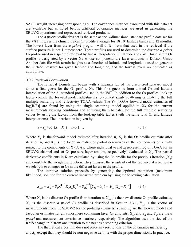
SAGE weight increasing correspondingly. The covariance matrices associated with this data set are available but as noted below, artificial covariance matrices are used in generating the SBUV/2 operational and reprocessed retrieval products.

The a priori profile data set is the same as the 3-dimensional standard profile data set for the V8T. It gives the climatological O3 profile averages for 18 10º latitude bands and 12 months. The lowest layer from the a priori program will differ from that used in the retrieval if the surface pressure is not 1 atmosphere. These profiles are used to determine the discrete a priori O3 profile used in a specific retrieval by linear interpolation in latitude and day. This discrete O3 profile is designated by a vector XA whose components are layer amounts in Dobson Units. Another data file with terrain heights as a function of latitude and longitude is used to generate the surface pressure for given latitude and longitude, and the lowest layers are truncated as appropriate. 3.3.2 Retrieval Formulation The retrieval formulation begins with a linearization of the discretized forward model about a first guess for the O3 profile, X0. This first guess is from a total O3 and latitude interpolation of the 21 standard profiles used in the V8T. In addition to the O3 profiles, look up tables contain the forward model adjustments to convert single scattering estimate to the full multiple scattering and reflectivity TOAA values. The Y0 [TOAA forward model estimates of log(R/F)] are found by using the single scattering model applied to X0 for the current measurements viewing conditions and adjusting them to calculate the full multiple scattering values by using the factors from the look-up table tables (with the same total O3 and latitude interpolations). The linearization is given by

Y =Yn + Kn (X − Xn ) n=0,1,… (3.3) Where Yn is the forward model estimate after iteration n, Xn is the O3 profile estimate after iteration n, and Kn is the Jacobian matrix of partial derivatives of the components of Y with respect to the components of X (∂yi/∂xj where individual yi and xj represent log of TOAA for an SBUV/2 channel and an O3 pressure layer amount, respectively) evaluated at Xn. The partial derivative coefficients in K are calculated by using the O3 profile for the previous iteration (Xn) and constitute the weighting function. They measure the sensitivity of the radiance at a particular wavelength to changes in O3 in the different layers in the profile. The iterative solution proceeds by generating the optimal estimation (maximum likelihood) solution for the current linearized problem by using the following calculation

Xn+1 = XA + SAKT [KnSAKnT

+ SM]-1[YM − Yn ) – Kn (XA − Xn )] (3.4)

Where Xn is the discrete O3 profile from iteration n, Xn+1 is the new discrete O3 profile estimate, XA is the discrete a priori O3 profile as described in Section 3.3.1, YM is the vector of measurements from the SBUV/2 for the profiling channels; Yn and Kn are the forward model and Jacobian estimates for an atmosphere containing layer O3 amounts, Xn; and SA and SM are the a priori and measurement covariance matrices, respectively. The algorithm uses the size of the RMS change in X from one iteration to the next as a stopping criterion.

The theoretical algorithm does not place any restrictions on the covariance matrices SA and SM except that they should be non-negative definite with the proper dimensions. In practice,

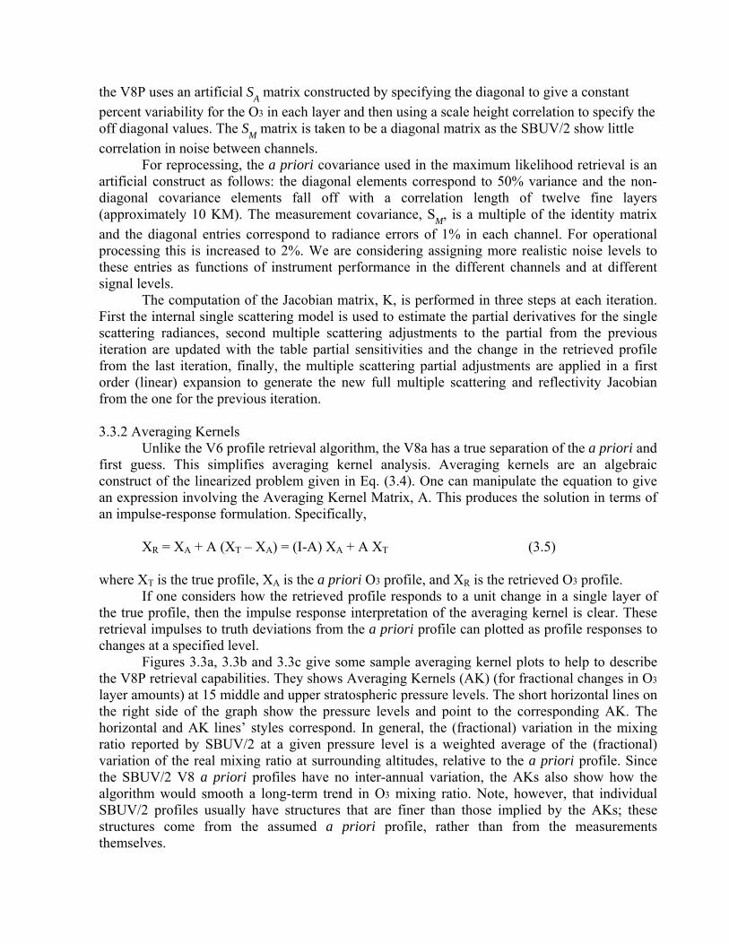
the V8P uses an artificial SA matrix constructed by specifying the diagonal to give a constant percent variability for the O3 in each layer and then using a scale height correlation to specify the off diagonal values. The SM matrix is taken to be a diagonal matrix as the SBUV/2 show little correlation in noise between channels.

For reprocessing, the a priori covariance used in the maximum likelihood retrieval is an artificial construct as follows: the diagonal elements correspond to 50% variance and the non-diagonal covariance elements fall off with a correlation length of twelve fine layers (approximately 10 KM). The measurement covariance, SM, is a multiple of the identity matrix and the diagonal entries correspond to radiance errors of 1% in each channel. For operational processing this is increased to 2%. We are considering assigning more realistic noise levels to these entries as functions of instrument performance in the different channels and at different signal levels.

The computation of the Jacobian matrix, K, is performed in three steps at each iteration. First the internal single scattering model is used to estimate the partial derivatives for the single scattering radiances, second multiple scattering adjustments to the partial from the previous iteration are updated with the table partial sensitivities and the change in the retrieved profile from the last iteration, finally, the multiple scattering partial adjustments are applied in a first order (linear) expansion to generate the new full multiple scattering and reflectivity Jacobian from the one for the previous iteration. 3.3.2 Averaging Kernels

Unlike the V6 profile retrieval algorithm, the V8a has a true separation of the a priori and first guess. This simplifies averaging kernel analysis. Averaging kernels are an algebraic construct of the linearized problem given in Eq. (3.4). One can manipulate the equation to give an expression involving the Averaging Kernel Matrix, A. This produces the solution in terms of an impulse-response formulation. Specifically,

XR = XA + A (XT – XA) = (I-A) XA + A XT (3.5)

where XT is the true profile, XA is the a priori O3 profile, and XR is the retrieved O3 profile. If one considers how the retrieved profile responds to a unit change in a single layer of

the true profile, then the impulse response interpretation of the averaging kernel is clear. These retrieval impulses to truth deviations from the a priori profile can plotted as profile responses to changes at a specified level.

Figures 3.3a, 3.3b and 3.3c give some sample averaging kernel plots to help to describe the V8P retrieval capabilities. They shows Averaging Kernels (AK) (for fractional changes in O3 layer amounts) at 15 middle and upper stratospheric pressure levels. The short horizontal lines on the right side of the graph show the pressure levels and point to the corresponding AK. The horizontal and AK lines’ styles correspond. In general, the (fractional) variation in the mixing ratio reported by SBUV/2 at a given pressure level is a weighted average of the (fractional) variation of the real mixing ratio at surrounding altitudes, relative to the a priori profile. Since the SBUV/2 V8 a priori profiles have no inter-annual variation, the AKs also show how the algorithm would smooth a long-term trend in O3 mixing ratio. Note, however, that individual SBUV/2 profiles usually have structures that are finer than those implied by the AKs; these structures come from the assumed a priori profile, rather than from the measurements themselves.

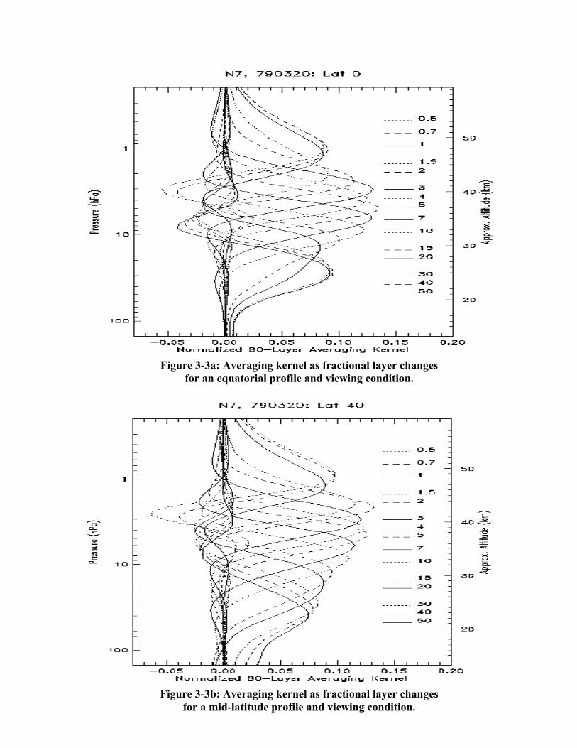
Figure 3-3a: Averaging kernel as fractional layer changes

for an equatorial profile and viewing condition.

Figure 3-3b: Averaging kernel as fractional layer changes

for a mid-latitude profile and viewing condition.

Figure 3-3c: Averaging kernels as fractional layer changes

for a high latitude profile and viewing condition.

Figure 3-3a shows typical AKs at the equator. The AKs show best resolution of ~6 km near 3 hPa, degrading to ~10 km at 1 and 20 hPa. Outside this range the retrieved profiles have little information. For example, the (fractional) variation in O3 mixing ratio seen at 0.5 hPa actually represents the (fractional) variation from the region around 1 hPa, and the variation around 50 hPa represents the variation from around 30 hPa.

Figure 3.3b shows typical AKs for March at 40N latitude. At this latitude the 50 hPa AK does capture some of the atmospheric variation, albeit with a FWHM resolution of ~11 km. In general, the upper AKs get progressively better as the solar zenith angle increases, and the lower AKs become better as the O3 density peak drops in altitude. Figure 3.3c shows typical AKs for March at 80N latitude. One can see the improvement in AKs for the upper portions of the profile, especially the 0.5, 0.7, 1, and 1.5 hPa AKs, in capturing the atmospheric variation more accurately than in Figs. 2 and 1, with better resolution of ~6 km at 0.7 hPa.

The AK results presented here use the SA and SM covariance matrices applied for the reprocessed product retrievals. The operational retrievals use an SM matrix with larger entries to allow for the greater uncertainty in the operational calibration. The averaging kernels for the operational implementation are slightly broader than those shown here. 3.4 Retrieval Algorithm Errors

The V8P combines backscattered ultraviolet measurements and a priori profile information in a maximum likelihood retrieval placing it in the same class of retrievals as V6A described in Bhartia et al. [1996]. The following list gives an overview of how errors will be reduced:

1. The V8P has new set of a priori profiles varying by month and latitude leading to better estimates in the troposphere (where SBUV/2 lacks retrieval information) and allowing simplified

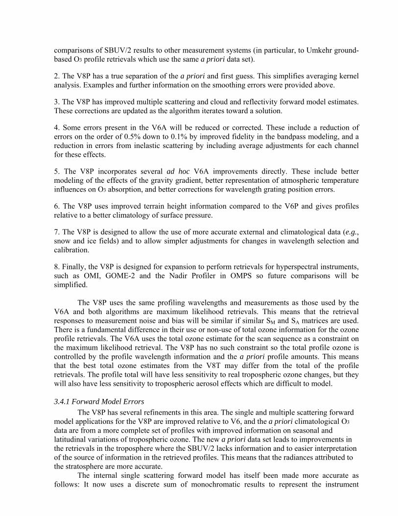
comparisons of SBUV/2 results to other measurement systems (in particular, to Umkehr ground-based O3 profile retrievals which use the same a priori data set).

2. The V8P has a true separation of the a priori and first guess. This simplifies averaging kernel analysis. Examples and further information on the smoothing errors were provided above.

3. The V8P has improved multiple scattering and cloud and reflectivity forward model estimates. These corrections are updated as the algorithm iterates toward a solution.

4. Some errors present in the V6A will be reduced or corrected. These include a reduction of errors on the order of 0.5% down to 0.1% by improved fidelity in the bandpass modeling, and a reduction in errors from inelastic scattering by including average adjustments for each channel for these effects.

5. The V8P incorporates several ad hoc V6A improvements directly. These include better modeling of the effects of the gravity gradient, better representation of atmospheric temperature influences on O3 absorption, and better corrections for wavelength grating position errors.

6. The V8P uses improved terrain height information compared to the V6P and gives profiles relative to a better climatology of surface pressure.

7. The V8P is designed to allow the use of more accurate external and climatological data (e.g., snow and ice fields) and to allow simpler adjustments for changes in wavelength selection and calibration.

8. Finally, the V8P is designed for expansion to perform retrievals for hyperspectral instruments, such as OMI, GOME-2 and the Nadir Profiler in OMPS so future comparisons will be simplified.

The V8P uses the same profiling wavelengths and measurements as those used by the V6A and both algorithms are maximum likelihood retrievals. This means that the retrieval responses to measurement noise and bias will be similar if similar SM and SA matrices are used. There is a fundamental difference in their use or non-use of total ozone information for the ozone profile retrievals. The V6A uses the total ozone estimate for the scan sequence as a constraint on the maximum likelihood retrieval. The V8P has no such constraint so the total profile ozone is controlled by the profile wavelength information and the a priori profile amounts. This means that the best total ozone estimates from the V8T may differ from the total of the profile retrievals. The profile total will have less sensitivity to real tropospheric ozone changes, but they will also have less sensitivity to tropospheric aerosol effects which are difficult to model. 3.4.1 Forward Model Errors

The V8P has several refinements in this area. The single and multiple scattering forward model applications for the V8P are improved relative to V6, and the a priori climatological O3 data are from a more complete set of profiles with improved information on seasonal and latitudinal variations of tropospheric ozone. The new a priori data set leads to improvements in the retrievals in the troposphere where the SBUV/2 lacks information and to easier interpretation of the source of information in the retrieved profiles. This means that the radiances attributed to the stratosphere are more accurate.

The internal single scattering forward model has itself been made more accurate as follows: It now uses a discrete sum of monochromatic results to represent the instrument

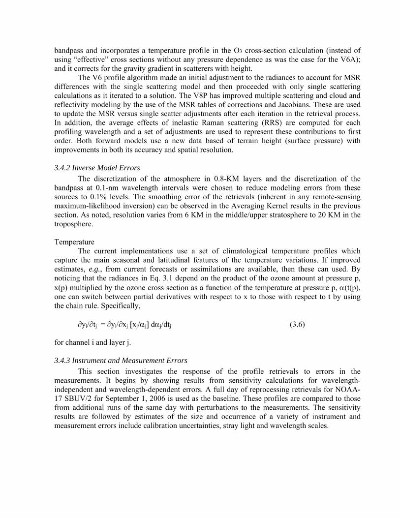
bandpass and incorporates a temperature profile in the O3 cross-section calculation (instead of using “effective” cross sections without any pressure dependence as was the case for the V6A); and it corrects for the gravity gradient in scatterers with height.

The V6 profile algorithm made an initial adjustment to the radiances to account for MSR differences with the single scattering model and then proceeded with only single scattering calculations as it iterated to a solution. The V8P has improved multiple scattering and cloud and reflectivity modeling by the use of the MSR tables of corrections and Jacobians. These are used to update the MSR versus single scatter adjustments after each iteration in the retrieval process. In addition, the average effects of inelastic Raman scattering (RRS) are computed for each profiling wavelength and a set of adjustments are used to represent these contributions to first order. Both forward models use a new data based of terrain height (surface pressure) with improvements in both its accuracy and spatial resolution. 3.4.2 Inverse Model Errors

The discretization of the atmosphere in 0.8-KM layers and the discretization of the bandpass at 0.1-nm wavelength intervals were chosen to reduce modeling errors from these sources to 0.1% levels. The smoothing error of the retrievals (inherent in any remote-sensing maximum-likelihood inversion) can be observed in the Averaging Kernel results in the previous section. As noted, resolution varies from 6 KM in the middle/upper stratosphere to 20 KM in the troposphere.

Temperature

The current implementations use a set of climatological temperature profiles which capture the main seasonal and latitudinal features of the temperature variations. If improved estimates, e.g., from current forecasts or assimilations are available, then these can used. By noticing that the radiances in Eq. 3.1 depend on the product of the ozone amount at pressure p, x(p) multiplied by the ozone cross section as a function of the temperature at pressure p, α(t(p), one can switch between partial derivatives with respect to x to those with respect to t by using the chain rule. Specifically,

∂yi/∂tj = ∂yi/∂xj [xj/αj] dαj/dtj (3.6) for channel i and layer j. 3.4.3 Instrument and Measurement Errors

This section investigates the response of the profile retrievals to errors in the measurements. It begins by showing results from sensitivity calculations for wavelength-independent and wavelength-dependent errors. A full day of reprocessing retrievals for NOAA-17 SBUV/2 for September 1, 2006 is used as the baseline. These profiles are compared to those from additional runs of the same day with perturbations to the measurements. The sensitivity results are followed by estimates of the size and occurrence of a variety of instrument and measurement errors include calibration uncertainties, stray light and wavelength scales.

Figure 3-4: Difference in retrieval responses for ±1% uniform measurement errors at all profiling wavelengths at 16 latitudes (every 10° from 75S to 75N)

Figure 3-4 shows the effects of a uniform shift in the calibration of all the profile wavelength measurement channels. The thick solid line gives the paired results for 45N latitude when all channels are increased by 1% or all channels are deceased by 1%. The dotted lines give the paired results for other the full range of latitudes covered by the SBUV/2, 80S to 80N. The retrieval algorithm interprets a 1% increase in the radiances at all profiling channels at 45N as a decrease in the middle and upper stratospheric ozone amounts of approximately 2%, little change in the lower stratosphere, and an increase in the tropospheric ozone amounts of 1%.

Figure 3-5 shows the effects of -0.5% shifts in individual channels for six profiling wavelength channels – 273 nm, 283 nm, 288 nm, 292 nm, 298 nm and 302 nm — for a retrieval at 45N latitude. The six curves go from the shortest channel to the longest in the following order; Thick Solid, Thick Dotted, Thick Dashed, Thin Solid, Thin Dotted, Thin Dashed. In general, the larger retrieval differences are found higher in the atmosphere for the shorter wavelengths and lower in the atmosphere for the longer ones. These features will follow the pattern of the contribution function shown in Fig 3-1, moving higher with increases in SZA or ozone amounts. The SA and SM matrices were in their reprocessing configuration for these sensitivity tests.

Figure 3-5: Difference in retrieval response for -0.5% measurement errors at individual profile wavelengths – 273, 283, 288, 292, 298 and 302-nm channels for the 273-nm to

302-nm channels at 45N latitude.

Radiance/Irradiance Calibration The measurement errors modeled in Figs. 3-4 & 3-5 were chosen because they are representative of the types of uncertainties expected in the TOAA calibration for the SBUV/2 instruments, that is, errors in the overall calibration of all the channels combined with errors in the relative calibration of individual channels. Details on the calibration of the SBUV/2 instruments are beyond the scope of this ATBD. Material on the methods for maintaining this calibration and estimates of the success of their application can be found in the following articles and their references: Herman et al. [1991], Bhartia et al. [1995], Hilsenrath et al. [1995], Cebula and DeLand [1998], Flynn et al. [2000], Huang et al. [2003], Deland et al. [2002], and Flynn et al. [2006].

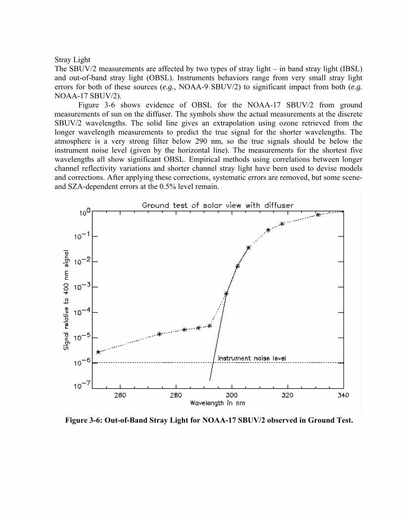
Stray Light The SBUV/2 measurements are affected by two types of stray light – in band stray light (IBSL) and out-of-band stray light (OBSL). Instruments behaviors range from very small stray light errors for both of these sources (e.g., NOAA-9 SBUV/2) to significant impact from both (e.g. NOAA-17 SBUV/2).

Figure 3-6 shows evidence of OBSL for the NOAA-17 SBUV/2 from ground measurements of sun on the diffuser. The symbols show the actual measurements at the discrete SBUV/2 wavelengths. The solid line gives an extrapolation using ozone retrieved from the longer wavelength measurements to predict the true signal for the shorter wavelengths. The atmosphere is a very strong filter below 290 nm, so the true signals should be below the instrument noise level (given by the horizontal line). The measurements for the shortest five wavelengths all show significant OBSL. Empirical methods using correlations between longer channel reflectivity variations and shorter channel stray light have been used to devise models and corrections. After applying these corrections, systematic errors are removed, but some scene- and SZA-dependent errors at the 0.5% level remain.

Figure 3-6: Out-of-Band Stray Light for NOAA-17 SBUV/2 observed in Ground Test.

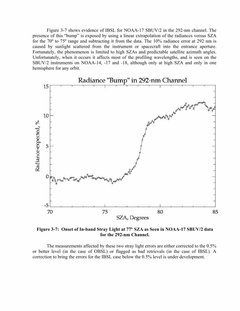
Figure 3-7 shows evidence of IBSL for NOAA-17 SBUV/2 in the 292-nm channel. The presence of this “bump” is exposed by using a linear extrapolation of the radiances versus SZA for the 70º to 75º range and subtracting it from the data. The 10% radiance error at 292 nm is caused by sunlight scattered from the instrument or spacecraft into the entrance aperture. Fortunately, the phenomenon is limited to high SZAs and predictable satellite azimuth angles. Unfortunately, when it occurs it affects most of the profiling wavelengths, and is seen on the SBUV/2 instruments on NOAA-14, -17 and -18, although only at high SZA and only in one hemisphere for any orbit.

Figure 3-7: Onset of In-band Stray Light at 77° SZA as Seen in NOAA-17 SBUV/2 data for the 292-nm Channel.

The measurements affected by these two stray light errors are either corrected to the 0.5% or better level (in the case of OBSL) or flagged as bad retrievals (in the case of IBSL). A correction to bring the errors for the IBSL case below the 0.5% level is under development.

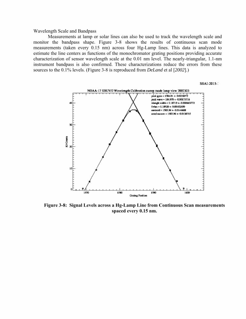
Wavelength Scale and Bandpass Measurements at lamp or solar lines can also be used to track the wavelength scale and

monitor the bandpass shape. Figure 3-8 shows the results of continuous scan mode measurements (taken every 0.15 nm) across four Hg-Lamp lines. This data is analyzed to estimate the line centers as functions of the monochromator grating positions providing accurate characterization of sensor wavelength scale at the 0.01 nm level. The nearly-triangular, 1.1-nm instrument bandpass is also confirmed. These characterizations reduce the errors from these sources to the 0.1% levels. (Figure 3-8 is reproduced from DeLand et al [2002].)

Figure 3-8: Signal Levels across a Hg-Lamp Line from Continuous Scan measurements spaced every 0.15 nm.

3.5 References Ball Aerospace & Technology Corporation, Algorithm Theoretical Basis Document (ATBD)

Nadir Profile Ozone) for the Ozone Mapping and Profiler Suite (OMPS)of the National Polar-Orbiting Operational Environmental Satellite System (NPOESS) Program, Document Number – IN0092A-108 CI Number – SS0052Am January 2002.

Bates, D.R., “Rayleigh scattering by air,” Planet. Sp. Sci., 32, 785-790, 1984. Bhartia, P.K., et al., “Applications of the Langley plot method to the calibration of SBUV

instrument on Nimbus-7 satellite,” J. Geophys. Res., 100, 2997-3004, 1995. Bhartia, P.K., et al., “Algorithm for the estimation of vertical profiles from the backscattered

ultraviolet technique,” J. Geophys. Res. 101, 18,793-18,806, 1996. Cebula, R.P., & DeLand, M.T., “Comparisons of the NOAA-11 SBUV/2, UARS SOLSTICE,

and UARS SUSIM Mg II solar activity proxy indexes,” Solar Physics, 177, 117–132, 1998.

Chapman, S., “The absorption and dissociative or ionizing effect of monochromatic radiation in an atmosphere on a rotating earth,” Proc. Phy. Soc. (London), 43, 483-501, 1931.

Deland, M.T., et al., NOAA-17 SBUV/2 (Flight Model#6) Activation and Evaluation Phase (A&E) Report, SSAI Document #SSAI-2015-180-MD-2002-02, 2002.

Fleig, A.J., et al., Nimbus 7 Solar Backscatter Ultraviolet (SBUV) Ozone Products User's Guide, NASA Reference Publication 1234, 1990.

Flynn, L.E., et al., 2000, ”Internal validation of SBUV/2 ozone vertical profile data sets,” Proceedings of the Quadrennial Ozone Symposium, Sapporo,. 75-76.

Flynn, L.E. et al., “Characterization of Operational Solar Backscatter Ultraviolet Insruments at the U.S. NOAA,” Proceedings of ACVE-3, ESA, Frascati Italy, December 4-7, 2006.

Frederick, J.E, R.P. Cebula, & D.F. Heath, “Instrument characterization for the detection of long-term changes in stratospheric ozone: An analysis of the SBUV/2 radiometer,” J. Atmos. Oceanic Technol., 3, 472-480, 1986.

Gleason, J.F, & R.D. McPeters, “Correction to the Nimbus 7 solar backscatter ultraviolet data in the "nonsync" period (Feb. 1987 to June 1990),” J. Geophys. Res., 100, 16,873-16,877, 1995.

Heath, D.F., et al., “The solar backscatter ultraviolet and total ozone mapping spectrometer (SBUV/TOMS) for Nimbus G,” Optical Engineering, 14, 323-331, 1975.

Heath, D.F., et al., ''Comparison of Spectral Radiance Calibrations of SSBUV-2 Satellite Ozone Monitoring Instruments using Integrating Sphere and Flat-Plate Diffuser Technique,'' Metrologia, 30, 259-264, 1993.

Herman, J.R., et al., “A new self-calibration method applied to TOMS and SBUV backscattered ultraviolet data to determine long-term global ozone change,” J. Geophys. Res., 96, 7531-7545, 1991.

Hilsenrath, E., et al., “Calibration of the NOAA-11 Solar Backscatter Ultraviolet (SBUV/2) Ozone Data Set from 1989 to 1993 using In-Flight Calibration Data and SSBUV,” J. Geophys. Res., 100, 1351-1366, 1995.

Huang, L.K., et al., “Determination of NOAA-11 SBUV/2 radiance sensitivity drift based on measurements of polar ice cap radiance,” Int. J. Remote Sensing, 24(2),305-314, 2003.

Meijer, Y., et al., “Evalution of global ozone monitoring experiment (GOME) ozone profiles from nine different algorithms, J. Geophys. Res., 111, D21306, doi: 10.1029/2005JD006778, 2006.

Rodgers, C.D., “Retrieval of atmospheric temperature and composition from remote measuremets of thermal radiation,” Rev. Geophys. Space Phys., 14, 609-624, 1976.

Rodgers, C.D., The Characterization and Error Analysis of Profiles Retrieved from Remote Sounding Measurements, J. Geophys. Res., 95, 5587-5595, 1990.

Web References The Solar Backscatter Ultraviolet instrument (SBUV/2) measurements fly on the NOAA Polar-orbiting Operation Environmental Satelllites (POES). Information on these sensors and products is available in sections 3.8, 7.4 and 9.7 of the NOAA-KLM User’s Guide at

http://www2.ncdc.noaa.gov/docs/klm/Activation and evaluation reports and other calibration documents can be found at

http://www.orbit.nesdis.noaa.gov/smcd/spb/calibration/icvs/sbuvdoc.htmlCalibration and validation monitoring can be found in the ultraviolet instrument links at

http://www.orbit.nesdis.noaa.gov/smcd/spb/calibration/icvs/index.htmlAdditional monitoring information and the V8 Fortran code are available from links at

http://www.orbit.nesdis.noaa.gov/smcd/spb/ozone/ftp://www.orbit.nesdis.noaa.gov/pub/smcd/spb/ozone/code

Additional documentation and product validation are contained on theV8P data DVD available at http://disc.sci.gsfc.nasa.gov/data/datapool/TOMS/DVD-ROMs/

The following documents with information on the V8T and V8P implementation in the operational processing at NOAA are available from NOAA/NESDIS: Solar Backscattered Ultraviolet Radiometer (SBUV/2) Operational Ozone Product System

Version 8, System Maintenance Manual, Dec. 2006, Prepared by Q. Zhao & J. Selekof. Solar Backscattered Ultraviolet Radiometer (SBUV/2) Operational Ozone Product System

Version 8, System Description Document, Dec. 2006, Prepared by Q. Zhao & J. Selekof. Solar Backscattered Ultraviolet Radiometer (SBUV/2) Operational Ozone Product System

Version 8, Interface Control Document, Dec. 2006, Prepared by Q. Zhao & J. Selekof.