Technical White Paper

Runoff Coefficient Evaluation

For Volumetric BMP Sizing

May 29, 2015

CTSW-TM-15-312.03.01

California Department of Transportation Division of Environmental Analysis

Stormwater Program 1120 N Street, Sacramento, California 95814

http://www.dot.ca.gov/hq/env/stormwater/index.htm

Form DEA F 001 (11-07) Reproduction of completed page authorized

CALTRANS Technical Report Documentation Page 1. Report No.

CTSW-TM-15-312.03.01

2. Type of Report

Technical Memorandum

3. Report Phase and Edition

Final

4. Title and Subtitle

Runoff Coefficient Evaluation for Volumetric BMP Sizing

5. Report Date

May 29, 2015

6. Copyright Owner(s)

California Department of Transportation

7. Caltrans Project Coordinator

Bala Nanjundiah

8. Performing Organization Names and Addresses

Office of Water Programs California State University, Sacramento 6000 J Street, 1001 Modoc Hall Sacramento, CA 95816 http://www.owp.csus.edu/

9. Task Order No.

003 Amendment No. N/A

10. Contract No.

43A0312

11. Sponsoring Agency Name and Address

California Department of Transportation Sacramento, CA 95814

12. Caltrans Functional Reviewers:

Design: Mike Marti, Sean Penders, Robert Schott, Tim Sobelman DEA: Bhaskar Joshi, Mark Keisler, Bala Nanjundiah, Mike Rogers

13. Supplementary Notes

14. External Reviewers

None

15. Abstract

Methods used to transform rainfall depth into runoff volume for sizing volumetric stormwater BMPs are identified and explained. This includes a cursory evaluation of the current method used by Caltrans, along with an initial inventory of other methods used by various municipalities and departments of transportation (DOTs). Only the basic theory, assumptions, and suitability to the Caltrans NPDES Permit sizing requirements are provided for each method.

16. Key Words

Volumetric runoff coefficient, curve number, stormwater, runoff volume

17. Distribution Statement

18. No. of pages

26

iii

ACKNOWLEDGMENTS

The following individuals are acknowledged for their contribution toward this project:

Christian Carleton Brian Currier

iv

DISCLAIMER

Any statements expressed in these materials are those of the individual authors and do not necessarily represent the views of CALTRANS, which takes no responsibility for any statement made herein. CALTRANS has not independently verified the results, conclusions or claims presented herein. No reference made in this publication to any specific method, product, process, or service constitutes or implies an endorsement, recommendation, or warranty thereof by CALTRANS. The materials are for general information only and do not represent a finding of fact, standard of CALTRANS, nor are they intended as a reference in purchase specifications, contracts, regulations, statutes, or any other legal document. CALTRANS makes no representation or warranty of any kind, whether expressed or implied, concerning the accuracy, completeness, suitability, or utility of any information, apparatus, product, or process discussed in this publication, and assumes no liability therefore. This information should not be used without first securing competent advice with respect to its suitability for any general or specific application. Anyone utilizing this information assumes all liability arising from such use, including but not limited to infringement of any patent or patents.

Technical Memoranda are used for timely documentation and communication of preliminary results, interim reports, or more localized or special purpose information that may not have received formal outside peer reviews or detailed editing.

Software applications are provided by CALTRANS “as is” and any express or implied warranties, including, but not limited to, the implied warranties of merchantability and fitness for a particular purpose are disclaimed. In no event shall CALTRANS be liable for any direct, indirect, incidental, special, exemplary, or consequential damages (including, but not limited to, procurement of substitute goods or services; loss of use, data, or profits; or business interruption) however caused and on any theory of liability, whether in contract, strict liability, or tort (including negligence or otherwise) arising in any way out of the use of this software, even if advised of the possibility of such damage.

Copyright (2015) California Department of Transportation

All Rights Reserved

1

BACKGROUND In 2012, the State Water Resources Control Board (SWRCB) issued the California Department of Transportation (Caltrans) a statewide National Pollutant Discharge Elimination System (NPDES) stormwater permit (Order No. 2012-0011-DWQ, NPDES No. CAS 000003)(Caltrans NPDES Permit 2013). The Permit specifies sizing treatment control Best Management Practices (BMPs) for the 85th percentile, 24-hour storm event, which is much smaller than the typical storm size used for drainage design.

Certain aspects of the current Caltrans method used to transform rainfall depth to runoff volume may result in the oversizing of volumetric stormwater BMPs. This technical white paper is intended to provide a cursory evaluation of the current method used by Caltrans and to provide an initial inventory of other methods used by various municipalities and departments of transportation (DOTs) around the country. Only the basic theory, assumptions, and suitability to the Caltrans NPDES Permit sizing requirements will be provided for each method.

DRAINAGE VS. STORMWATER QUALITY DESIGN The basic hydrology and hydraulic principles are the same whether designing a drainage system or a stormwater quality treatment BMP. However, these two types of runoff designs have very different design goals and philosophies that must be recognized in order to meet performance objectives.

The design goal for drainage systems is to protect human health and property from flooding. In order to accomplish this goal the design must have the capacity to convey runoff from a large storm, such as a 25-year recurrence interval storm. Furthermore, drainage systems are predominantly engineered to handle a specified flow rate instead of a runoff volume.

The design goal for stormwater quality treatment BMPs is to treat the many small storms that collectively transport the majority of the runoff pollutants. Treating larger and less frequent storms creates a diminishing return on installation and maintenance costs. An optimized design capacity is typically a storm that has a recurrence interval of less than 2 years. Because the runoff volume from these smaller water quality design storms is much less than the volume that is produced by a larger drainage system design storm, initial abstraction (losses from interception, depressional storage, etc. that occur before runoff begins) is a more significant factor in estimating the transformation of precipitation to runoff for small storms than it is for larger storms. In addition, the initial abstraction volume can be a large percentage of the total precipitation volume. As the amount of precipitation increases, the initial abstraction volume stays constant, which causes it to become an increasingly smaller percentage of the total precipitation volume until it reaches a point where it can be considered negligible for very large storms.

Due to differences in the targeted storm sizes between drainage design and stormwater quality treatment BMP design, the methods used to estimate runoff cannot necessarily be interchanged. Dhakal et al. (2012) recognized that volumetric-based coefficients should not be used to predict peak discharge rates, and furthermore observed that volumetric coefficients derived from data are weakly correlated to the rate-based coefficients available in the literature. This finding helps highlight the importance of recognizing that rate-based coefficients and volume-based coefficients are not the same and as such should not be used in place of each other. However, this distinction does not mean that drainage design and stormwater quality treatment BMP design requirements cannot be achieved on the

2

same project. Proper BMP design should include bypass and overflow elements that allow the BMP to meet the drainage design requirements.

This white paper focuses on the design storm requirements of the Caltrans NPDES Permit and therefore limits its investigation to methods available for sizing volumetric BMPs for the 85th percentile, 24-hour storms across the state which approximates a <2-year return period.

CURRENT CALTRANS METHOD The current guidance provided by Caltrans for calculating volumetric stormwater treatment BMP sizes is provided in the Storm Water Quality Handbooks: Project Planning and Design Guide (PPDG; Caltrans 2012b), Section 2.4.2.2, “Treatment BMP Use and Placement Considerations.” For projects with project initiation documents (PIDs) approved prior to July 1, 2013, the PPDG specifies using the 85th percentile runoff capture ratio or maximized volume approach1 and refers the designer to the Basin Sizer design tool (Caltrans 2007) to perform the calculations. Projects with PIDs approved after this date will use the 85th percentile 24-hour storm event in the new NPDES order.

In Basin Sizer version 1.45 and earlier, a runoff depth equivalent is estimated by multiplying the rainfall depth for the selected location by a user-provided composite runoff coefficient. The runoff depth equivalent can then be multiplied by the drainage area to get the runoff volume. However, both the PPDG and Basin Sizer guidance are unclear on what input values to use for the composite runoff coefficient for the drainage area. The Highway Design Manual (HDM; Caltrans 2014) is also silent on how to estimate runoff volumes for sizing stormwater BMPs, and provides no guidance on selecting an appropriate runoff coefficient. Without explicit guidance for volumetric coefficients, Caltrans designers use the HDM Figure 819.2A, “Runoff Coefficients for Undeveloped Areas,” and Table 819.2B, “Runoff Coefficients for Developed Areas.”

In 2013, the Caltrans Infiltration Tools version 3.01 (Caltrans 2013a; Caltrans 2013b) was released. The Infiltration Tools use Basin Sizer to get a design storm depth (not a runoff depth). If using Basin Sizer version 1.45 and earlier a composite runoff coefficient of 1.0 must be used; in version 1.46 (the most recent) the runoff coefficient input has been removed so that only a rainfall depth is provided. Regardless of which version of Basin Sizer is used to get the rainfall depth, the transformation of rainfall to runoff is calculated within the Infiltration Tools by multiplying the rainfall depth by the drainage area and a runoff coefficient. Two runoff coefficients are used: the first coefficient is 0.9, for impervious areas; the second is based on user inputs for the pervious areas taken directly from the HDM, Figure 819.2B.

Both the original Basin Sizer method and the newer Infiltration Tools/Basin Sizer method use runoff coefficients from the HDM. These coefficients are intended to be used with the rational method for estimating peak design discharge (i.e., flow rate). Often referred to as C values, they represent the ratio between rainfall intensity and peak flow rate. This allows them to act as the transformation function within the rational method to estimate flow rate (i.e., volume per time) from precipitation intensity (i.e., depth per time). Furthermore, the rational method and its coefficients are intended for use in estimating peak runoff from large storm events (typically the 10-year recurrence interval and larger).

1 The PPDG sizing method will be revised to match the 2013 Caltrans NPDES Permit requirements of the 85th percentile, 24-hour storm event (Order No 2012-0011-DWQ).

3

This is in contrast to the design objective for sizing a volumetric BMP, which needs to estimate runoff volume as a function of precipitation depth for much smaller and more frequent storm events.

While use of the current HDM runoff coefficient values in the sizing of volumetric BMPs is not necessarily appropriate, the resulting design sizes are permit-compliant since these rate-based coefficients tend to oversize BMPs relative to BMPs sized with a more appropriate coefficient from one of the techniques described later in this technical white paper.

SMALL STORM HYDROLOGY METHOD (SSHM) The Small Storm Hydrology Method (SSHM) is currently the most widely used non-computerized model for the calculation of stormwater volume runoff (see Appendix A). There are several different forms of the equation used by various municipalities across the nation, but, ultimately, they can all be described by Equation 1. It is based on the simple mass balance principle that a proportion of the rainfall on a drainage area translates into runoff.

∀𝑅= 𝑅𝑣𝑃𝑃 Equation 1 Where: ∀𝑅 = Runoff Volume [L3] 𝑅𝑣 = Volumetric Runoff Coefficient [unitless] 𝑃 = Precipitation Depth [L] 𝑃 = Drainage Area [L2] In the SSHM, the Volumetric Runoff Coefficient (Rv) is defined as the ratio of runoff volume to precipitation volume (Equation 2). It can either be assigned based on drainage area characteristics or it can be calculated as an area-weighted composite.

𝑅𝑣 =∀𝑅∀𝑃

Equation 2

Where: ∀𝑃 = Precipitation Volume [L3] = 𝑃𝑃 Three approaches have emerged as the preferred techniques of obtaining Rv values: 1) linear regression equations based on the percent impervious, 2) polynomial equations based on percent impervious, and 3) look-up tables based on land use/cover and precipitation depth. All of these approaches are empirical and the results are sensitive to the precipitation distribution and land uses in the locations where the data were collected.

Linear Regression Equations Using data from the National Urban Runoff Program (NURP), Driscoll (1983) calculated the mean Rv at over 50 monitored sites. He was able to show that the majority of the variation within the mean Rv values for each site was attributed to the amount of urbanization or imperviousness within the drainage area. While working for the Metropolitan Washington Council of Governments, Schueler used a subset of Driscoll’s data and adding a few more sites to compile a table of 44 sites with percent impervious, mean Rv, and median Rv values (WMWRPB 1987). Based on this composite data set, Schueler used simple linear regression to derive Equation 3, which predicts a mean Rv based on the percent impervious.

4

𝑅𝑣 = 0.05 + 0.009(𝐼) 𝑅2 = 0.71 Equation 3 Where: 𝑅𝑣 = Volumetric Runoff Coefficient [unitless] 𝐼 = Percent Impervious of Drainage Area (0-100) The majority of the municipal design manuals reviewed for this white paper (Appendix A) use Equation 3. While not published in the literature, if outliers are removed from the data set Equation 4 is obtained. About 20% of the municipal design manuals reviewed used this form of the equation.

𝑅𝑣 = 0.015 + 0.0092(𝐼) 𝑅2 = 0.86 Equation 4 Reese (2006) proposed using the median Rv instead of the mean Rv (Equation 5) to develop an alternate relationship. This alternative, while not used prolifically in professional practice, has validity because it is more robust for data sets containing outliers. Outliers caused by measurement errors are inevitable when measuring small runoff events, so using median values reduces the impact of erroneous measurements. As a result, Equation 5 provides a practical and intuitive result that shows that highly pervious catchments do not produce runoff from the smallest storms considered.

𝑅𝑣 = 0.0091(𝐼)− 0.0204 𝑅2 = 0.85 Equation 5 Figure 1 displays a graph of the Schueler data and the three linear regression equations derived from the data. The right side of the plot area (white side) identifies the range of percent impervious within which Caltrans typically has to design and size stormwater BMPs. It is important to recognize that only about 20% of the data used to derive these relationships are within this range. It is also important to recognize that the fundamental assumption about all three equations is that Rv only changes with percent impervious and is not affected by any other factors such as storm characteristics (e.g., intensity, depth, duration). The one shortcoming of Equation 5 then is that due to the constraints of fitting a straight line through the data, sites with very low percent imperviousness result in a negative Rv which is not physically possible, so results should be limited to positive values. However, this limitation would not likely impact the highway environment because the percent impervious typically remains well above 50% where treatment BMPs are required.

Figure 1 – Comparison of the linear regression equations developed from the Schueler (1987) data.

5

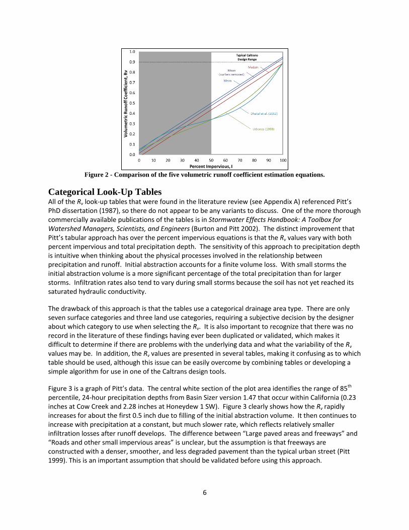
Polynomial Equations Recognizing that there may be a better model for the NURP data, Urbonas (1999) proposed a third order polynomial equation to estimate Rv (Equation 6; Figure 2). This equation is presented in Urban Runoff Quality Management (WEF and ASCE 1998) and included in the California Stormwater BMP Handbook: New Development and Redevelopment (CASQA 2003). Also, according to Dhakal et al. (2012), this equation was used in the 2010 Drainage Criteria Manual for the Denver Urban Drainage and Flood Control District.2 Equation 6 was derived using median Rv values from 60 NURP sites.

𝑅𝑣 = 0.858 �𝐼

100�3− 0.78 �

𝐼100

�2

+ 0.774 �𝐼

100� + 0.04 𝑅2 = 0.72

Equation 6

Note: Variables used in the original published equation have been adjusted for internal

consistency within this technical white paper.

Equation 6 is more complicated than Equations 3-5 and provides some valuable insight. As shown in Figure 2, Equation 6 follows a similar trend for the lower Rv values estimated by Equation 5 for areas with a higher percentage of impervious surfaces. It also rectifies the negative Rv values of Equation 5 for areas with little to no impervious surfaces.

Dhakal et al. (2012) added 45 sites from Texas to the 60 NURP sites to derive Equation 7.

𝑅𝑣 = 1.843 �𝐼

100�3− 2.275 �

𝐼100

�2

+ 1.289 �𝐼

100� + 0.036 𝑅2 = 0.57

Equation 7

Note: Variables used in the original published equation have been adjusted for internal

consistency within this white paper.

Perhaps the most important point that the third order polynomial equations illustrate is the degree to which Rv may not be a linear function. The slope of the lines in Figure 2 represents the rate of change in Rv with respect to percent impervious. The linear regression equations have a constant slope, therefore Rv is directly proportional to percent impervious. However, the Urbonas and Dhakal et al. approaches have more complex relationships between Rv and percent impervious. The slope of the line is greatest in both of these equations for high percent impervious (>75%). This is the range where the infiltration in the pervious areas is overwhelmed by the excess runoff from the impervious surfaces. The Dhakal et al. (2012) equation has more curvature because of how the additional Texas data points are clustered. This factor introduces a bias into Equation 7, making its applicability questionable for areas outside of where the additional data were collected.

2 The equation appears to have been removed in the 2013 edition of the manual.

6

Figure 2 - Comparison of the five volumetric runoff coefficient estimation equations.

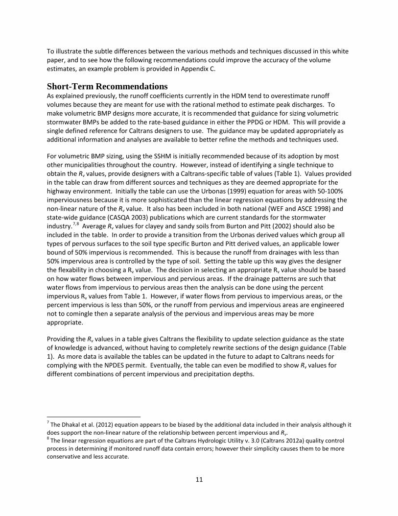
Categorical Look-Up Tables All of the Rv look-up tables that were found in the literature review (see Appendix A) referenced Pitt’s PhD dissertation (1987), so there do not appear to be any variants to discuss. One of the more thorough commercially available publications of the tables is in Stormwater Effects Handbook: A Toolbox for Watershed Managers, Scientists, and Engineers (Burton and Pitt 2002). The distinct improvement that Pitt’s tabular approach has over the percent impervious equations is that the Rv values vary with both percent impervious and total precipitation depth. The sensitivity of this approach to precipitation depth is intuitive when thinking about the physical processes involved in the relationship between precipitation and runoff. Initial abstraction accounts for a finite volume loss. With small storms the initial abstraction volume is a more significant percentage of the total precipitation than for larger storms. Infiltration rates also tend to vary during small storms because the soil has not yet reached its saturated hydraulic conductivity.

The drawback of this approach is that the tables use a categorical drainage area type. There are only seven surface categories and three land use categories, requiring a subjective decision by the designer about which category to use when selecting the Rv. It is also important to recognize that there was no record in the literature of these findings having ever been duplicated or validated, which makes it difficult to determine if there are problems with the underlying data and what the variability of the Rv values may be. In addition, the Rv values are presented in several tables, making it confusing as to which table should be used, although this issue can be easily overcome by combining tables or developing a simple algorithm for use in one of the Caltrans design tools.

Figure 3 is a graph of Pitt’s data. The central white section of the plot area identifies the range of 85th percentile, 24-hour precipitation depths from Basin Sizer version 1.47 that occur within California (0.23 inches at Cow Creek and 2.28 inches at Honeydew 1 SW). Figure 3 clearly shows how the Rv rapidly increases for about the first 0.5 inch due to filling of the initial abstraction volume. It then continues to increase with precipitation at a constant, but much slower rate, which reflects relatively smaller infiltration losses after runoff develops. The difference between “Large paved areas and freeways” and “Roads and other small impervious areas” is unclear, but the assumption is that freeways are constructed with a denser, smoother, and less degraded pavement than the typical urban street (Pitt 1999). This is an important assumption that should be validated before using this approach.

7

Furthermore, the fact that freeways have Rv values greater than pitched roofs is questionable and indicates that results were generated from a limited data set.

Figure 3 – Pitt’s volumetric runoff coefficients for different rainfall depths (data from Burton and Pitt 2002).

CURVE NUMBER (CN) METHOD The Soil Conservation Service (SCS), now known as the Natural Resources Conservation Service (NRCS), originally developed their hydrology techniques based on unit hydrograph theory and curve numbers in the 1940s and 1950s (USDA-NRCS 2004). Hydrologic calculations were originally done by hand, but in the 1960s the process was coded into a computer program that was documented in Technical Release 20 (TR-20), Computer Program for Project Formulation Hydrology (USDA-SCS 1992). Utilizing output from TR-20, the SCS was then able to develop further simplified techniques for estimating runoff and peak discharges in Technical Release 55 (TR-55), Urban Hydrology for Small Watersheds (USDA-NRCS 1986). Two separate hydrologic methods are utilized within TR-20 and TR-55. The first is the curve number (CN) method that calculates a storm event’s direct runoff depth based on a precipitation depth and land use/cover. The second method is the dimensionless unit hydrographs that convert the direct runoff depth to a hydrograph with a peak flow rate (ASCE/EWRI 2009).

Today, TR-55 provides the most common form of the CN method used with stormwater calculations. Its theory is based on the use of a CN to estimate the potential maximum retention after runoff begins (Equation 8) and the initial abstraction (Equation 9).

𝑆 =1000𝐶𝐶

− 10 Equation 8

Where: 𝑆 = Potential Maximum Retention After Runoff Begins (in) 𝐶𝐶 = Curve Number (unitless)

𝐼𝑎 = 0.2𝑆 Equation 9 Where: 𝐼𝑎 = Initial Abstraction (in) The theoretical basis for TR-55 then ties S and Ia together using Equation 10, which is a hyperbolic equation to estimate the runoff depth.

8

𝑄 =(𝑃 − 𝐼𝑎)2

(𝑃 − 𝐼𝑎) + 𝑆

Equation 10

Where: 𝑄 = Runoff Depth (in) 𝑃 = Precipitation Depth (in) One of the benefits of using the TR-55 CN method to comply with the Caltrans NPDES Permit requirements is that the method is based completely on 24-hour storm events, which conveniently matches with the Permit’s 85th percentile, 24-hour storm event sizing requirement. However, the NRCS (2009) makes a point of identifying limitations of the TR-55 method, including accuracy issues with less than 0.5 inch of runoff. Furthermore, Claytor and Schueler (1996) state that the CN method underestimates the runoff volume for small storms less than 2 inches, and provide explanations in their Table 2.10.3 This is the reason why most agencies do not use the TR-55 CN method to estimate runoff volume. The NRCS also points out that the 0.2S relationship is based on data from agricultural watersheds, which has the potential to generate erroneous Ia estimates in urban watersheds. This can be easily observed by assuming a CN of 98 for impervious areas, which calculates an Ia of 0.04 inch (1 mm) using Equation 9. Observation of any paved surface during a light rain event would suggest that this Ia is small since the adhesion and cohesion of the water on the roadway alone would likely account for at least this much of a loss even before depressional storage or initial infiltration are considered.

Figure 4 provides curves of Rv values calculated using the TR-55 CN method as a function of precipitation depth for different percent imperviousness. The percent impervious assumes a CN of 98 for impervious surfaces and 70 for pervious surfaces. While the exact values may not be correct, the outcome of this analysis is very insightful. All of the curves have an Rv of zero when the precipitation equals Ia. For precipitation greater than Ia the curves are smooth, well behaved, and probably accurate. For precipitation less than Ia the curves display asymptotic behavior approaching an Rv of infinity at a precipitation of zero. This is the likely reason why NRCS suggests a minimum runoff depth of 0.5 inch. However, Figure 4 illustrates that this anomaly lessens with increased CN such that a site with 100 percent impervious area is virtually unaffected. While further investigation is needed, it appears that this limitation may not be a significant factor for the types of percent impervious areas that Caltrans typically designs.

3 Claytor and Schueler’s conclusions are based on an unpublished manuscript presented by Pitt at a conference in 1994. A copy of this manuscript could not be located to include its contents in this technical white paper, yet many of the municipal design manuals listed in Appendix A reference it when explaining why the CN method should not be used to estimate runoff volumes for small storms. See Pitt, Robert E. 1994. Small Storm Hydrology. Presented at Design of Stormwater Quality Management Practices, Madison, WI, May 17-19.

9

Figure 4 – Volumetric runoff coefficients for varying precipitation depths and percent impervious

(CN 70 to 98).

Using the same assumptions for percent impervious (CN range from 70 to 98), Figure 5 shows Rv as a function of percent impervious for different precipitation depths. As the depth increases, the line straightens out, similar to the three linear regression equations. Conversely, smaller precipitation depths have more curvature, similar to the polynomial equations, because they are more affected by the initial abstraction. As discussed earlier, the exact values of the lines may not be correct, but this graph provides theoretical support for non-linear solutions, such as the third order polynomial equations, for smaller stormwater quality design storms, and the linear regression equations for larger storms.

Figure 5 - Volumetric runoff coefficients for varying percent impervious (CN 70 to 98) and

precipitation depths.

While the TR-55 CN methodology may not be appropriate for use with all stormwater quality design storms, the underlying CN methodology is still a valid model. Fortunately, the computer version (WinTR-554) eliminates these issues because it uses an algorithm based on TR-20 (USDA-NRCS 2009). Further 4 Available at http://www.nrcs.usda.gov/wps/portal/nrcs/detailfull/national/water/?cid=stelprdb1042901

10

investigation into the applicability of WinTR-55 for sizing stormwater quality treatment BMPs in the highway environment would be needed before this method could be adopted.

COMPUTER MODELS The two most common computer models used to model stormwater runoff (i.e., runoff volume, infiltration, etc.) are the US EPA Storm Water Management Model (SWMM)5 and the joint US EPA and USGS Hydrological Simulation Program FORTRAN (HSPF).6 The reason for the popularity of these models is that they can both perform continuous simulation. Due to the significantly more advanced and complex nature of these types of models, continuous simulation computer models are not within the scope of this white paper. However, they are mentioned here because of the potential to use them for either verification or calibration of the other models discussed.

For single event design storm analysis, the USACE HEC-HMS and the USGS WinTR-55 are the most common. WinTR-55 is used more often for stormwater BMP sizing, likely because of its ties to the original TR-55 method.

RECOMMENDATIONS The rate-based runoff coefficients from the HDM were not developed for small storm volumetric BMP sizing. In order to calculate the most accurate volume estimate, both percent impervious and precipitation depth should be utilized. To help illustrate this point, Appendix B contains a table that compares the Rv values between the different techniques presented. The TR-55 column shows how the Rv values decrease not only with percent impervious, like the other techniques, but also with the precipitation depth. The Appendix B table spans the full range of California’s 85th percentile, 24-hour rainfall depths.

Currently, there is no simple method that is widely accepted by the stormwater industry that accounts for both percent impervious and precipitation depth when dealing with small storms. The CN method is not appropriate for smaller storms, and other methods reviewed for Rv estimation do not account for differences with precipitation depth. As a way to work around this shortcoming in knowledge, the recommendations are divided into short-term and long-term recommendations.

The short-term recommendations can be implemented immediately and are based on the current state of knowledge. They identify a way to use existing methods in such a way that they can be appropriately utilized by Caltans in the highway environment. If Caltrans decides that a more accurate method for estimating runoff volumes is needed then the long-term recommendations have been provided. These recommendations require further investigation and analysis to be implemented. However, they have the potential to provide a more accurate solution that is calibrated to the Caltrans highway environment.

5 Available at http://www.epa.gov/nrmrl/wswrd/wq/models/swmm/ 6 Available at http://water.usgs.gov/software/HSPF/

11

To illustrate the subtle differences between the various methods and techniques discussed in this white paper, and to see how the following recommendations could improve the accuracy of the volume estimates, an example problem is provided in Appendix C.

Short-Term Recommendations As explained previously, the runoff coefficients currently in the HDM tend to overestimate runoff volumes because they are meant for use with the rational method to estimate peak discharges. To make volumetric BMP designs more accurate, it is recommended that guidance for sizing volumetric stormwater BMPs be added to the rate-based guidance in either the PPDG or HDM. This will provide a single defined reference for Caltrans designers to use. The guidance may be updated appropriately as additional information and analyses are available to better refine the methods and techniques used.

For volumetric BMP sizing, using the SSHM is initially recommended because of its adoption by most other municipalities throughout the country. However, instead of identifying a single technique to obtain the Rv values, provide designers with a Caltrans-specific table of values (Table 1). Values provided in the table can draw from different sources and techniques as they are deemed appropriate for the highway environment. Initially the table can use the Urbonas (1999) equation for areas with 50-100% imperviousness because it is more sophisticated than the linear regression equations by addressing the non-linear nature of the Rv value. It also has been included in both national (WEF and ASCE 1998) and state-wide guidance (CASQA 2003) publications which are current standards for the stormwater industry.7,8 Average Rv values for clayey and sandy soils from Burton and Pitt (2002) should also be included in the table. In order to provide a transition from the Urbonas derived values which group all types of pervous surfaces to the soil type specific Burton and Pitt derived values, an applicable lower bound of 50% impervious is recommended. This is because the runoff from drainages with less than 50% impervious area is controlled by the type of soil. Setting the table up this way gives the designer the flexability in choosing a Rv value. The decision in selecting an appropriate Rv value should be based on how water flows between impervious and pervious areas. If the drainage patterns are such that water flows from impervious to pervious areas then the analysis can be done using the percent impervious Rv values from Table 1. However, if water flows from pervious to impervious areas, or the percent impervious is less than 50%, or the runoff from pervious and impervious areas are engineered not to comingle then a separate analysis of the pervious and impervious areas may be more appropriate.

Providing the Rv values in a table gives Caltrans the flexibility to update selection guidance as the state of knowledge is advanced, without having to completely rewrite sections of the design guidance (Table 1). As more data is available the tables can be updated in the future to adapt to Caltrans needs for complying with the NPDES permit. Eventually, the table can even be modified to show Rv values for different combinations of percent impervious and precipitation depths.

7 The Dhakal et al. (2012) equation appears to be biased by the additional data included in their analysis although it does support the non-linear nature of the relationship between percent impervious and Rv. 8 The linear regression equations are part of the Caltrans Hydrologic Utility v. 3.0 (Caltrans 2012a) quality control process in determining if monitored runoff data contain errors; however their simplicity causes them to be more conservative and less accurate.

12

Table 1: Recommended initial table of volumetric runoff coefficients (Rv)

Description Volumetric Runoff

Coefficient (Rv) Source 100% Impervious 0.89 Urbonas 1999 90% Impervious 0.73 Urbonas 1999 80% Impervious 0.60 Urbonas 1999 70% Impervious 0.49 Urbonas 1999 60% Impervious 0.41 Urbonas 1999 50% Impervious 0.34 Urbonas 1999 Clayey Soils1 0.22 Burton and Pitt 2002 Sandy Soils1 0.03 Burton and Pitt 2002

1 Value for an average California 85th percentile, 24-hour storm event depth of 1.26 inches.

Long-Term Recommendations The following long-term recommendations are provided in order of easiest to most extensive. The estimated duration of time needed to implement each of these recommendations is included.

• Data mine the Caltrans Stormwater Data Archive (SDA) to develop a California highway-specific Rv data set. Use the data to develop an equation that estimates Rv as a function of percent impervious and precipitation depth. (Estimated duration: 4-8 months after the SDA flow data review is completed)

• Re-calculate the Rv linear regression and polynomial equations using only the NURP sites with percent impervious > 50%, and add a confidence interval to each prediction equation. Results can then be compared against studies in the Caltrans SDA. (Estimated duration: 1-2 months)

• Investigate the validity of using the WinTR-55 computer program to access the TR-20 method to calculate the runoff volumes. Using a computer program will be especially helpful for drainage areas with both connected and disconnected impervious areas. Please note that in a preliminary investigation, WinTR-55 (TR-20) estimated a substantially lower Rv than the original TR-55 method. This result will need to be explained. (Estimated duration: 6-8 months)

• Use the TR-20 method to develop a new relationship between Ia and S for pavement-dominated drainage areas and small storms, as recommended by the NRCS. This method can be used in place of the TR-55 equations. (Estimated duration: 6-12 months after the investigation into the validity of using the WinTR-55 computer program has been completed)

13

REFERENCES ASCE/EWRI Curve Number Hydrology Task Committee. 2009. Curve Number Hydrology:

State of the Practice. Edited by Richard H. Hawkins, Timothy J. Ward, Donald E. Woodward and Joseph A. Van Mullen. Reston, VA: American Society of Civil Engineers.

Burton, G. Allen, and Robert Pitt. 2002. Stormwater Effects Handbook: A Toolbox for Watershed Managers, Scientists, and Engineers. Boca Raton, FL: Lewis Publishers.

California Department of Transportation (Caltrans). 2007. Caltrans Basin Sizer Methodologies. User manual. CTSW-RT-07-180.04.1. Caltrans. Sacramento, CA.

California Department of Transportation (Caltrans). 2012a. Caltrans Hydrologic Utility v. 3.0 User Manual. CTSW-SA-10-239.02.02. Caltrans, Division of Environmental Analysis. Sacramento, CA.

California Department of Transportation (Caltrans). 2012b. Storm Water Handbooks Project Planning and Design Guide. CTSW-RT-10-254.03. Caltrans, Office of Storm Water Managment - Design. Sacramento, CA.

California Department of Transportation (Caltrans). 2013a. T-1 Checklist Infiltration Tools v. 3.01, Technical Reference. CTSW-SA-12-239.09.05. Caltrans, Division of Environmental Analysis. Sacramento, CA.

California Department of Transportation (Caltrans). 2013b. T-1 Checklist Infiltration Tools v. 3.01, User Manual. CTSW-SA-12-239.09.04. Caltrans, Divison of Environmental Analysis. Sacramento, CA.

California Department of Transportation (Caltrans). 2014. Highway Design Manual. Caltrans. Sacramento, CA.

California Stormwater Quality Association (CASQA). 2003. California Stormwater BMP Handbook: New Development and Redevelopment. CASQA. Menlo Park, CA.

Claytor, R.A., and T.R. Schueler. 1996. Design of Stormwater Filtering Systems. Chesapeake Research Consortium, Inc. Solomons, MD.

Dhakal, Nirajan, Xing Fang, Theodore G. Cleveland, David B. Thompson, William H. Asquith, and Luke J. Marzen. 2012. Estimation of Volumetric Runoff Coefficients for Texas Watersheds Using Land-Use and Rainfall-Runoff Data. Journal of Irrigation & Drainage Engineering 138 (1):43-54. doi: 10.1061/(asce)ir.1943-4774.0000368.

Driscoll, Eugene D. 1983. Rainfall/Runoff Relationships from the NURP Urban Runoff Data Base. paper Presented at Stormwater and Quality Models Users Group Meeting, Montreal, Quebec, Sep 8-9.

National Pollutant Discharge Elimination System (NPDES) Statewide Storm Water Permit Waste Discharge Requirements (WDRs) for State of California Department of Transportation. California State Water Resources Control Board (SWRCB). Order No. 2012-0011-DWQ, NPDES No. CAS000003 (2013).

Pitt, Robert E. 1987. “Small Storm Urban Flow and Particulate Washoff Contributions to Outfall Discharges.” PhD diss., Department of Civil Engineering, University of Wisconsin, Madison. University Microfilms (123.3523).

Pitt, Robert E. 1999. Small Storm Hydrology and Why it is Important for the Design of Stormwater Control Practices. In New Applications in Modeling Urban Water Systems, edited by William James, 61-92. Guelph, ON Canada: CHI.

Urbonas, Ben R. 1999. Design of a Sand Filter for Stormwater Quality Enhancement. Water Environment Research 71 (1):102-113. doi: 10.2307/25045180.

14

USDA-Natural Resources Conservation Service (NRCS). 1986. Urban Hydrology for Small Watersheds, Technical Release 55, Second Edition. Technical Release. 210-VI-TR-55. US Department of Agriculture, Natural Resources Conservation Service, Conservation Engineering Division. Washington, DC.

USDA-Natural Resources Conservation Service (NRCS). 2004. WinTR-20 User Guide (Draft). US Department of Agriculture, Natural Resources Conservation Service, Conservation Engineering Division. Washington, DC.

USDA-Natural Resources Conservation Service (NRCS). 2009. Small Watershed Hydrology WinTR-55 User Guide. US Department of Agriculture, Natural Resources Conservation Service, Conservation Engineering Division. Washington, DC.

USDA-Soil Conservation Service (SCS). 1992. Computer Program for Project Formulation Hydrology TR-20. US Department of Agriculture, Soil Conservation Service, Hydrology Unit and Technology Development Support. Washington, DC.

Washington Metropolitan Water Resources Planning Board (WMWRPB). 1987. Controlling Urban Runoff: A Practical Manual for Planning and Desgning Urban BMPs. Metropolitan Washington Council of Governments, Department of Environmental Programs. Washington, D.C.

Water Environment Federation (WEF), and American Society of Civil Engineers (ASCE). 1998. Urban Runoff Quality Management, WEF Manual of Practice No. 23 and ASCE Manual and Report on Engineering Practice No. 87. Alexandria, VA and Reston, VA: WEF and ASCE.

A-1

APPENDIX A List of some of the municipality design manuals using the Small Storm Hydrology Method.

Design Manual Method/Technique Table/Curve

Fort Wayne, Indiana, Stormwater Design and Specification Manual (2009)

SSHM with Rv = 0.05+0.009(I)

N

Lawrence Village, Georgia, Stormwater Design Manual SSHM with Rv = 0.05+0.009(I)

N

New York State Stormwater Management Design Manual (2010)*

SSHM with Rv = 0.05+0.009(I)

Y

Indianapolis, Indiana, Stormwater Specifications Manual (2011) SSHM with Rv = 0.05+0.009(I)

N

Boone County, Michigan, Stormwater Design Manual SSHM with Rv = 0.05+0.009(I)

N

Dallastown, Pennsylvania, Stormwater Management (2005) SSHM with Rv = 0.05+0.009(I)

N

Andover, Massachusetts, Stormwater Management and Erosion Control Regulations (2009)

SSHM with Rv = 0.05+0.009(I)

N

Department of Transportation, Hawaii Post Construction BMP Training (2012)

SSHM with Rv = 0.05+0.009(I)

N

Minnesota Pollution Control Agency, The Simple Method for Estimating Phosphorus Export

SSHM with Rv = 0.05+0.009(I)

N

Georgia Coastal Stormwater Supplement (2009) SSHM with Rv = 0.05+0.009(I)

N

Salisbury, Maryland, Wastewater Treatment Plant PER SSHM with Rv = 0.05+0.009(I)

N

Maryland Stormwater Design Manual (2000)* SSHM with Rv = 0.05+0.009(I)

N

Alaska Storm Water Guide (2011)* SSHM with Rv = 0.05+0.009(I)

N

Newton, Kansas, Post Construction Best Management Practices Manual

SSHM with Rv = 0.05+0.009(I)

Y

Virginia Stormwater Management Handbook (2013)* SSHM with Rv = 0.05+0.009(I)

N

Madisonville, Kentucky, Storm Water Management SSHM with Rv = 0.05+0.009(I)

N

Columbia, Missouri, Stormwater Management and Water Quality Manual (2013)

SSHM with Rv = 0.05+0.009(I)

Y

North Carolina Division of Water Quality, Stormwater Best Management Practices Manual (2007)*

SSHM with Rv = 0.05+0.009(I)

N

New Hampshire Stormwater Manual: Volume 2 (2008)* SSHM with Rv = 0.05+0.009(I)

N

A-2

Design Manual Method/Technique Table/Curve

City of Mexico Stormwater Manual SSHM with Rv = 0.05+0.009(I)

N

Knox County, Tennessee, Stormwater Management Manual SSHM with Rv = 0.015 + 0.0092(I )

N

Franklin, Tennessee, Water Quality Policy and Procedures SSHM with Rv = 0.015 + 0.0092(I )

N

Elizabethton, Tennessee, Water Quality BMP Manual (2008) SSHM with Rv = 0.015 + 0.0092(I )

Y

Rutherford, Tennessee, Stormwater Best Management Practices (2006)

SSHM with Rv = 0.015 + 0.0092(I )

N

Washington State Dept. of Transportation, Highway Runoff Manual (2011)

Continuous Simulation N

Pennsylvania Department of Environmental Protection, Pennsylvania Stormwater Best Management Practices Manual (2006)

Look-Up Table Y

Southeast Michigan Council of Governments, Low Impact Development Manual for Michigan: A Design Guide for Implementers and Reviewers (2008)*

Look-Up Table Y

*Statewide guidance utilized by DOTs

B-1

APPENDIX B

Comparison of volumetric runoff coefficients (Rv) obtained using different methods.

Current Caltrans Practice

(HDM Table 819.2B )1

Small Storm Hydrology Method TR-55

Linear Regression Equations Polynomial Equations Categorical Look-Up

Tables Eq. 3 Eq. 4 Eq. 5 Eq. 6 Eq. 7 Categorical CN

Range of 85% 24-hr CA PCP

(in) % Imp

Schueler (1987) -Mean-

Schueler (1987) w/o

Outliers -Mean-

Reese (2006)

-Median- Urbonas (1999)

Dhakal et al. (2012) Pitt (1987)2 NRCS3

2.28 (Honeydew4)

100% 0.95 0.95 0.94 0.89 0.89 0.89 0.86 0.90 75% 0.79 0.73 0.71 0.66 0.54 0.50 0.72 0.62 50% 0.63 0.50 0.48 0.43 0.34 0.34 0.59 0.41

1.00 100% 0.95 0.95 0.94 0.89 0.89 0.89 0.71 0.79

75% 0.79 0.73 0.71 0.66 0.54 0.50 0.58 0.38 50% 0.63 0.50 0.48 0.43 0.34 0.34 0.46 0.18

0.62 (Sac)

100% 0.95 0.95 0.94 0.89 0.89 0.89 0.65 0.70 75% 0.79 0.73 0.71 0.66 0.54 0.50 0.53 0.21 50% 0.63 0.50 0.48 0.43 0.34 0.34 0.42 0.05

0.23 (Cow Crk5)

100% 0.95 0.95 0.94 0.89 0.89 0.89 0.54 0.40 75% 0.79 0.73 0.71 0.66 0.54 0.50 0.44 0.00 50% 0.63 0.50 0.48 0.43 0.34 0.34 0.33 0.00

1 Assumes coefficients of 0.95 for impervious surfaces and 0.30 for pervious surfaces 2 Assumes coefficients from Roads and other small impervious areas for impervious surfaces and Clayey soils for pervious surfaces as shown in Figure 3 3 Assumes CN of 98 for impervious surfaces and 70 for pervious surfaces 4 Largest 85% 24-hour precipitation station from Basin Sizer 5 Smallest 85% 24-hour precipitation station from Basin Sizer

C-1

APPENDIX C

Example Problem

Project Description

The project is a new 3-lane section of highway located in Sacramento County. One of the drainages in the project is a 0.3-mile (1633 feet) stretch with 2 new lanes (12 feet each), a 3-foot impermeable shoulder with a curb, and a cut slope that is approximately 27 feet wide. A slope intercept drain is installed at the top of the cut slope to prevent run-on. Two of the lanes, the shoulder, and the cut slope drain to a newly proposed BMP that needs to be sized volumetrically. The surrounding soil is a Type C soil with native grasses. The 85th percentile, 24-hour rainfall depth for Sacramento is 0.62 inch. Figure C1 is a schematic of this example problem.

Figure C1 – Schematic of Example Problem

Solution

1. Calculate areas

The contributing drainage area (CDA) to the BMP consists of the two lanes, impermeable shoulder, and the area below the slope intercept drain.

C-2

𝐶𝐶𝑃 = (12 𝑓𝑓 + 12 𝑓𝑓 + 3 𝑓𝑓 + 27 𝑓𝑓) × �1633 𝑓𝑓 ×1 𝑎𝑎

43560 𝑓𝑓2� = 2 𝑎𝑎

The net new impervious (NNI) area consists of only the two lanes and impermeable shoulder.

𝐶𝐶𝐼 𝑃𝐴𝐴𝑎 = (12 𝑓𝑓 + 12 𝑓𝑓 + 3 𝑓𝑓) × �1633 𝑓𝑓 ×1 𝑎𝑎

43560 𝑓𝑓2� = 1 𝑎𝑎

The percent impervious for the CDA can now be calculated.

% 𝐼𝐼𝐼 = 𝐶𝐶𝐼 𝑃𝐴𝐴𝑎𝐶𝐶𝑃

× 100 =1 𝑎𝑎2 𝑎𝑎

× 100 = 50%

2. Volumetric Runoff Coefficients

The volumetric runoff coefficient (Rv) should be calculated for both the water quality volume (WQV) coming off of the NNI area (100% impervious) and the target capture volume coming off of the CDA (50% impervious). For comparison purposes, calculations from four of the most viable techniques are provided.

Current Caltrans Practice:

From the Caltrans Highway Design Manual (HDM), Table 819.2B, a conservative runoff coefficient for streets (impervious surface) is 0.95, and for unimproved areas (pervious surface) is 0.30. The composite runoff coefficient can then be calculated using an area-weighted approach:

𝐶100% = 0.95

𝐶 =𝐶1𝑃1 + 𝐶2𝑃2𝑃1 + 𝑃2

𝐶50% =(0.95 × 1 𝑎𝑎) + (0.30 × 1 𝑎𝑎)

1 𝑎𝑎 + 1 𝑎𝑎= 0.63

Reese (2006):

The Reese (2006) equation is a linear regression equation that estimates median Rv values based on the drainage area’s percent impervious.

𝑅𝑣 = 0.0091(𝐼)− 0.0204

𝑅𝑣 100% = 0.0091(100)− 0.0204 = 0.89

𝑅𝑣 50% = 0.0091(50) − 0.0204 = 0.43

Urbonas (1999):

C-3

The Urbonas (1999) equation is a third order polynomial equation that estimates median Rv values based on the drainage area’s percent impervious.

𝑅𝑣 = 0.858 �𝐼

100�3− 0.78 �

𝐼100

�2

+ 0.774 �𝐼

100� + 0.04

𝑅𝑣 100% = 0.858 �100100

�3− 0.78 �

100100

�2

+ 0.774 �100100

� + 0.04 = 0.89

𝑅𝑣 50% = 0.858 �50

100�3

− 0.78 �50

100�2

+ 0.774 �50

100�+ 0.04 = 0.34

TR-55 CN Method:

The TR-55 CN method uses curve numbers as the coefficient instead of volumetric runoff coefficients. From the Urban Hydrology for Small Watersheds (NRCS 1986), Table 2-2, a curve number for streets (impervious surface) is 98, and for a grassland/meadow area (pervious surface) is 70. The composite curve number can then be calculated on TR-55, Worksheet 2 using an area weighted approach:

𝐶𝐶 =𝐶𝐶1𝑃1 + 𝐶𝐶2𝑃2

𝑃1 + 𝑃2

𝐶𝐶100% = 98 → 𝑄0.62 𝑖𝑖 = 0.43 𝑖𝑖

𝑅𝑣 100% =𝑄𝑃

=0.43 𝑖𝑖0.62 𝑖𝑖

= 0.69

𝐶𝐶50% =(98 × 1 𝑎𝑎) + (70 × 1 𝑎𝑎)

1 𝑎𝑎 + 1 𝑎𝑎= 84 → 𝑄0.62 𝑖𝑖 = 0.027 𝑖𝑖

𝑅𝑣 50% =𝑄𝑃

=0.027 𝑖𝑖0.62 𝑖𝑖

= 0.043

3. Target Capture Volume

The target capture volume can now be calculated for the runoff coming off of the CDA.

Current Caltrans Practice:

∀= 0.63 × 0.62𝑖𝑖 �1𝑓𝑓

12𝑖𝑖� × 2𝑎𝑎 �

43560 𝑓𝑓2

1𝑎𝑎 � = 2836𝑓𝑓3

Reese (2006):

C-4

∀𝑅= 0.62𝑖𝑖 �1𝑓𝑓

12𝑖𝑖� × 0.43 × 2𝑎𝑎 �

43560 𝑓𝑓2

1𝑎𝑎 � = 1936𝑓𝑓3

Urbonas (1999):

∀𝑅= 0.62𝑖𝑖 �1𝑓𝑓

12𝑖𝑖� × 0.34 × 2𝑎𝑎 �

43560 𝑓𝑓2

1𝑎𝑎 � = 1530𝑓𝑓3

TR-55 CN Method:

𝑆 =1000𝐶𝐶

− 10 𝑄 =(𝑃 − 0.2𝑆)2

(𝑃 + 0.8𝑆)

𝑆 =1000

84− 10 = 1.90𝑖𝑖 𝑄 =

�0.62𝑖𝑖 − 0.2(1.90𝑖𝑖)�2

�0.62𝑖𝑖 + 0.8(1.90𝑖𝑖)�= 0.027𝑖𝑖

∀𝑅= 𝑄𝑃

∀𝑅= 0.027𝑖𝑖 �1𝑓𝑓

12𝑖𝑖� × 2𝑎𝑎 �

43560 𝑓𝑓2

1𝑎𝑎 � = 196𝑓𝑓3

4. Water Quality Volume

The water quality volume (WQV) can now be calculated for the runoff coming from the NNI area.

Current Caltrans Practice:

∀= 𝐶𝑃𝑃

∀= 0.95 × 0.62𝑖𝑖 �1𝑓𝑓

12𝑖𝑖� × 1𝑎𝑎 �

43560 𝑓𝑓2

1𝑎𝑎 � = 2138𝑓𝑓3

Small Storm Hydrology:

∀𝑅= 𝑃𝑅𝑣𝑃

Using Reese (2006):

∀𝑅= 0.62𝑖𝑖 �1𝑓𝑓

12𝑖𝑖� × 0.89 × 1𝑎𝑎 �

43560 𝑓𝑓2

1𝑎𝑎 � = 2003𝑓𝑓3

Using Urbonas (1999):

∀𝑅= 0.62𝑖𝑖 �1𝑓𝑓

12𝑖𝑖� × 0.89 × 1𝑎𝑎 �

43560 𝑓𝑓2

1𝑎𝑎 � = 2003𝑓𝑓3

C-5

TR-55 CN Method:

𝑆 =1000𝐶𝐶

− 10 𝑄 =(𝑃 − 0.2𝑆)2

(𝑃 + 0.8𝑆)

𝑆 =1000

98− 10 = 0.20𝑖𝑖 𝑄 =

�0.62𝑖𝑖 − 0.2(0.20𝑖𝑖)�2

�0.62𝑖𝑖 + 0.8(0.20𝑖𝑖)�= 0.431𝑖𝑖

∀𝑅= 𝑄𝑃

∀𝑅= 0.431𝑖𝑖 �1𝑓𝑓

12𝑖𝑖� × 1𝑎𝑎 �

43560 𝑓𝑓2

1𝑎𝑎 � = 1565𝑓𝑓3

5. Summary

Tables 1 and 2 provide a comparison of the runoff coefficients and resulting WQV and Target Capture Volumes using the four different methods.

Table 1 – Comparison of Runoff Coefficients

Surface Type

Current Caltrans

Practice (HDM Table 819.2B )

Eq. 5 Eq. 6 TR-55

Reese (2006)

-Median- Urbonas (1999)

NRCS

CN Rv

equivalent* Impervious (100%) 0.95 0.89 0.89 98 0.70 Composite (50%) 0.63 0.43 0.34 84 0.05 *For the condition of 0.62 inches in 24-hours

Table 2 – Comparison of Runoff Volumes

Volume Type

Current Caltrans

Practice (HDM Table 819.2B )

Eq. 5 Eq. 6 TR-55 Reese (2006)

-Median- Urbonas (1999)

NRCS Composite

CN Separated

Land Use CN Water Quality Volume 2138 2003 2003 1565 1565 Target Capture Volume 2836 1936 1530 196 1565

It is important to recognize that the composite CN used in the TR-55 method assumes that the impervious and pervious areas are homogeneously distributed throughout the drainage area. This results in an erroneously small Target Capture Volume for small, non-homogeneous drainages (196 ft2 for this example). A more appropriate approach for highways is to analyze the land uses separately and then add the resulting runoff volumes. For the 0.62 inch of rainfall with a pervious area CN of 70 there is no runoff, therefore the Target Capture Volume for this example is the same as the WQV.