Advances in Water Resources 59 (2013) 123–132

Contents lists available at SciVerse ScienceDirect

Advances in Water Resources

journal homepage: www.elsevier .com/ locate/advwatres

Robust numerical solution of the reservoir routing equation

0309-1708/$ - see front matter � 2013 Elsevier Ltd. All rights reserved.http://dx.doi.org/10.1016/j.advwatres.2013.05.013

⇑ Corresponding author.E-mail addresses: marcello.fiorentini@unimore.it (M. Fiorentini), stefano.orlan-

dini@unimore.it (S. Orlandini).URL: http://www.idrologia.unimore.it/orlandini (S. Orlandini).

Marcello Fiorentini, Stefano Orlandini ⇑Dipartimento di Ingegneria ‘‘Enzo Ferrari’’, Universitá degli Studi di Modena e Reggio Emilia, Strada Vignolese 905, 41125 Modena, Italy

a r t i c l e i n f o a b s t r a c t

Article history:Received 14 January 2013Received in revised form 13 April 2013Accepted 29 May 2013Available online 11 June 2013

Keywords:Surface runoffReservoirsFloods

The robustness of numerical methods for the solution of the reservoir routing equation is evaluated. Themethods considered in this study are: (1) the Laurenson–Pilgrim method, (2) the fourth-order Runge–Kutta method, and (3) the fixed order Cash–Karp method. Method (1) is unable to handle nonmonotonicoutflow rating curves. Method (2) is found to fail under critical conditions occurring, especially at the endof inflow recession limbs, when large time steps (greater than 12 min in this application) are used.Method (3) is computationally intensive and it does not solve the limitations of method (2). The limita-tions of method (2) can be efficiently overcome by reducing the time step in the critical phases of the sim-ulation so as to ensure that water level remains inside the domains of the storage function and theoutflow rating curve. The incorporation of a simple backstepping procedure implementing this controlinto the method (2) yields a robust and accurate reservoir routing method that can be safely used in dis-tributed time-continuous catchment models.

� 2013 Elsevier Ltd. All rights reserved.

1. Introduction

The term ‘‘reservoir routing’’ (or ‘‘storage routing’’) is used todenote the propagation of an inflow hydrograph through a reser-voir. Storage in surface reservoirs may be natural or man-made[12, p. 100]. Natural storage in the form of lakes, swamps and riv-ers have a strong influence on the flow from the catchment butdoes not regulate flow [19, p. 308]. Regulation in the water re-sources management sense requires man-made control structures.Reservoir storage refers to the part of the reservoir volume whichcan be used for flow regulation. A reservoir may be required to sup-ply water for power generation, irrigation, water supply, flood pro-tection, and recreational use. Each of these requirements of thereservoir imposes constraints on the operating policy. Many ofthese requirements contradict each other (e.g., power generationrequires a full reservoir or maximum head whereas flood protec-tion requires an empty reservoir). For flood protection in a multi-purpose reservoir a certain volume of the storage reservoir iskept empty, ready to receive water during the peak of the flood.The flow rate downstream is limited to a predetermined maximumvalue. The stored water is released after the flood peak has passed.Thus the reservoir receives all the water in excess of the designflow rate and the peak of the hydrograph is skimmed off and is de-layed by storage. This mechanism reduces the peak discharge rateof the downstream hydrograph but increases the baselength of the

hydrograph [16]. Predictions of the magnitude of the flood peak, itstime of occurrence, and the volume of water to be stored areneeded for the design of the reservoir. More in general, detaileddescriptions of the hydrologic interactions between reservoirsand regulated river systems are needed to determine structuraland nonstructural measures for flood protection and water re-sources management.

A reservoir can be modeled either as a large channel reach or asa pool [9]. While (distributed) channel routing may be needed todescribe the propagation of rapidly rising hydrographs (e.g., havingtime of rise less than 1 h) along very long (e.g., having lengthsgreater than 80 km) reservoirs, (lumped) pool routing is adequate(e.g., errors non exceeding 10%) in most of the cases [9]. Level poolrouting is a procedure for calculating the outflow hydrograph froma reservoir with a horizontal water surface, given its inflow hydro-graph and storage-outflow characteristics [4, p. 245]. The equa-tions governing reservoir dynamics can be combined to yield thenonlinear first-order ordinary differential equation

dSdt¼ IðtÞ � Qðt; SÞ; ð1Þ

where S is the volume of water stored in the reservoir, t is the time, Iis the inflow discharge, and Q is the outflow discharge, or the equiv-alent differential equation

dHdt¼ IðtÞ � Qðt;HÞ

AðHÞ ; ð2Þ

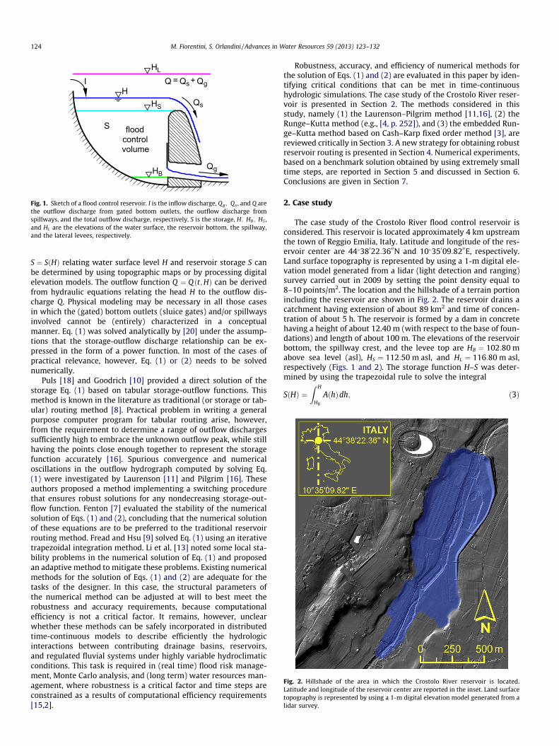
where H is the water surface level and A ¼ dS=dH is the watersurface area at elevation H. A sketch of the quantities involvedin level pool routing is shown in Fig. 1. The storage function

flood

volumecontrol

HB

HS Qs

HL

Qg

Qs Qg=Q +IH

S

Fig. 1. Sketch of a flood control reservoir. I is the inflow discharge, Qg ; Qs , and Q arethe outflow discharge from gated bottom outlets, the outflow discharge fromspillways, and the total outflow discharge, respectively, S is the storage, H; HB; HS ,and HL are the elevations of the water surface, the reservoir bottom, the spillway,and the lateral levees, respectively.

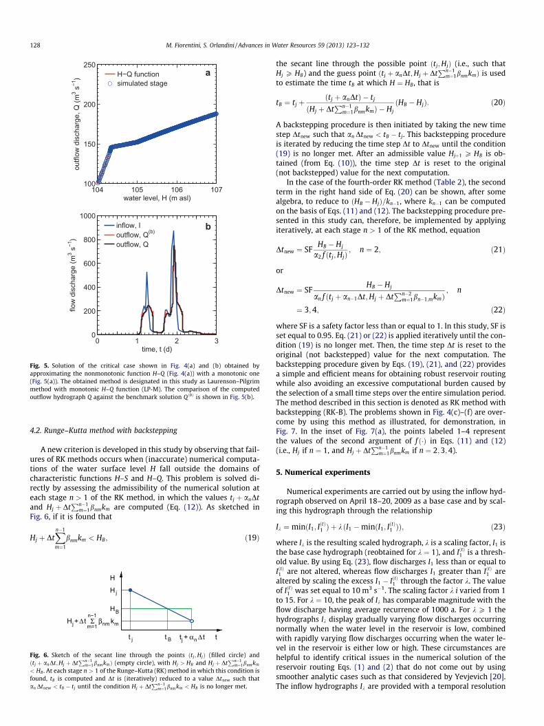
Fig. 2. Hillshade of the area in which the Crostolo River reservoir is located.Latitude and longitude of the reservoir center are reported in the inset. Land surfacetopography is represented by using a 1-m digital elevation model generated from alidar survey.

124 M. Fiorentini, S. Orlandini / Advances in Water Resources 59 (2013) 123–132

S ¼ SðHÞ relating water surface level H and reservoir storage S canbe determined by using topographic maps or by processing digitalelevation models. The outflow function Q ¼ Qðt;HÞ can be derivedfrom hydraulic equations relating the head H to the outflow dis-charge Q. Physical modeling may be necessary in all those casesin which the (gated) bottom outlets (sluice gates) and/or spillwaysinvolved cannot be (entirely) characterized in a conceptualmanner. Eq. (1) was solved analytically by [20] under the assump-tions that the storage-outflow discharge relationship can be ex-pressed in the form of a power function. In most of the cases ofpractical relevance, however, Eq. (1) or (2) needs to be solvednumerically.

Puls [18] and Goodrich [10] provided a direct solution of thestorage Eq. (1) based on tabular storage-outflow functions. Thismethod is known in the literature as traditional (or storage or tab-ular) routing method [8]. Practical problem in writing a generalpurpose computer program for tabular routing arise, however,from the requirement to determine a range of outflow dischargessufficiently high to embrace the unknown outflow peak, while stillhaving the points close enough together to represent the storagefunction accurately [16]. Spurious convergence and numericaloscillations in the outflow hydrograph computed by solving Eq.(1) were investigated by Laurenson [11] and Pilgrim [16]. Theseauthors proposed a method implementing a switching procedurethat ensures robust solutions for any nondecreasing storage-out-flow function. Fenton [7] evaluated the stability of the numericalsolution of Eqs. (1) and (2), concluding that the numerical solutionof these equations are to be preferred to the traditional reservoirrouting method. Fread and Hsu [9] solved Eq. (1) using an iterativetrapezoidal integration method. Li et al. [13] noted some local sta-bility problems in the numerical solution of Eq. (1) and proposedan adaptive method to mitigate these problems. Existing numericalmethods for the solution of Eqs. (1) and (2) are adequate for thetasks of the designer. In this case, the structural parameters ofthe numerical method can be adjusted at will to best meet therobustness and accuracy requirements, because computationalefficiency is not a critical factor. It remains, however, unclearwhether these methods can be safely incorporated in distributedtime-continuous models to describe efficiently the hydrologicinteractions between contributing drainage basins, reservoirs,and regulated fluvial systems under highly variable hydroclimaticconditions. This task is required in (real time) flood risk manage-ment, Monte Carlo analysis, and (long term) water resources man-agement, where robustness is a critical factor and time steps areconstrained as a results of computational efficiency requirements[15,2].

Robustness, accuracy, and efficiency of numerical methods forthe solution of Eqs. (1) and (2) are evaluated in this paper by iden-tifying critical conditions that can be met in time-continuoushydrologic simulations. The case study of the Crostolo River reser-voir is presented in Section 2. The methods considered in thisstudy, namely (1) the Laurenson–Pilgrim method [11,16], (2) theRunge–Kutta method (e.g., [4, p. 252]), and (3) the embedded Run-ge–Kutta method based on Cash–Karp fixed order method [3], arereviewed critically in Section 3. A new strategy for obtaining robustreservoir routing is presented in Section 4. Numerical experiments,based on a benchmark solution obtained by using extremely smalltime steps, are reported in Section 5 and discussed in Section 6.Conclusions are given in Section 7.

2. Case study

The case study of the Crostolo River flood control reservoir isconsidered. This reservoir is located approximately 4 km upstreamthe town of Reggio Emilia, Italy. Latitude and longitude of the res-ervoir center are 44�38022:3600N and 10�35009:8200E, respectively.Land surface topography is represented by using a 1-m digital ele-vation model generated from a lidar (light detection and ranging)survey carried out in 2009 by setting the point density equal to8–10 points/m2. The location and the hillshade of a terrain portionincluding the reservoir are shown in Fig. 2. The reservoir drains acatchment having extension of about 89 km2 and time of concen-tration of about 5 h. The reservoir is formed by a dam in concretehaving a height of about 12.40 m (with respect to the base of foun-dations) and length of about 100 m. The elevations of the reservoirbottom, the spillway crest, and the levee top are HB ¼ 102:80 mabove sea level (asl), HS ¼ 112:50 m asl, and HL ¼ 116:80 m asl,respectively (Figs. 1 and 2). The storage function H–S was deter-mined by using the trapezoidal rule to solve the integral

SðHÞ ¼Z H

HB

AðhÞdh; ð3Þ

M. Fiorentini, S. Orlandini / Advances in Water Resources 59 (2013) 123–132 125

where the water surface area A ¼ AðhÞ for h ¼ ½HB;H� is readilydetermined from the 1-m resolution digital elevation model shownin Fig. 2 by considering all the cells lying within the reservoir andhaving elevation less than or equal to h. The obtained storage func-tion H–S is shown in Fig. 3(a). The outflow discharge rating curve H–Q, determined from physical modeling, is shown in Fig. 3(b). It isnoted here that the obtained outflow discharge rating curve dis-plays an interval of H around the value of 104.70 m asl in whichthe outflow discharge Q decreases as the water surface level H in-creases. This is due to the transition from free surface flow to totallysubmerged flow through the bottom outlets. The storage volume atthe maximum design elevation of 114.68 m asl is about 3 � 106 m3,and the outflow discharge released by the reservoir under theseconditions is about 950 m3 s�1 (Fig. 3(a) and (b)).

3. Methods

The numerical methods for the solution of the reservoir Eqs. (1)and (2) can be grouped in two dominant classes. The first class isbased on the numerical approximation of the storage Eq. (1) ob-tained by using the trapezoidal rule, namely

Sjþ1 � Sj ¼Dt2

Ijþ1 þ Ij� �

� Qjþ1 þ Q j

� �� �; ð4Þ

where j is the counter of nodes tj ¼ jDt ðj ¼ 0;1;2; . . .Þ, along thetime domain, Dt is the time step, Sj; Ij, and Qj are the storage, theinflow discharge, and the outflow discharge, respectively, at timetj ðj ¼ 0;1;2; . . .Þ (e.g., [4, p. 246]). The traditional method men-tioned in Section 1 is obtained by putting Eq. (4) in the form

0

1

2

3

4

stor

age,

S (1

06 m

3 )

Δ0

εS

a

102 107 112 1170

500

1000

1500

2000

2500

outfl

ow d

isch

arge

, Q (m

3 s−

1 )

water level, H (m asl)

b

b

103 104 105 10660

120

180

240

Fig. 3. (a) Water level-storage (H–S) relationship obtained by applying Eq. (3) to thedigital elevation model reported in Fig. 2, and (b) water level-outflow discharge (H–Q) relationship obtained experimentally from a physical model of the Crostolo Riverreservoir. The inset in (b) highlights the region in which the H–Q function isnonmonotonic as a result of the transition from (open-channel) free surface topressurized pipe flow through the bottom outlets.

2Sjþ1

Dtþ Q jþ1 ¼ Ijþ1 þ Ij

� �þ 2Sj

Dt� Qj

� �ð5Þ

and by determining the unknown values Hjþ1; Sjþ1, and Qjþ1 fromtabular data mapping H and 2S=Dt þ Q [18,10,11,16,4,7]. This tradi-tional method is unconditionally stable, but it displays an accuracyevaluated on the Yevjevich’s [20] test case that is less than the sec-ond-order Runge–Kutta method [7]. Therefore, the traditionalmethod is not evaluated in the present study. An alternative meth-od based on Eq. (4) was introduced by Laurenson [11] and furtherdeveloped by Pilgrim [16]. This method, denoted shortly as ‘‘LPmethod,’’ is described in Section 3.1 and is evaluated in the presentstudy. The second class of methods is composed of explicit numer-ical solutions of Eq. (2). Runge–Kutta methods belong to this class[4,7]. Explicit Runge–Kutta methods were found by Fenton [7] toprovide the best solutions in terms of consistency, accuracy, andstability. The Runge–Kutta method, denoted shortly as ‘‘RK meth-od,’’ and the embedded Runge–Kutta method proposed by Cashand Karp [3], denoted shortly as ‘‘CK method,’’ are described in Sec-tions 3.2 and 3.3, respectively, and are evaluated in the presentstudy.

3.1. Laurenson–Pilgrim method

The LP method solves a variant of Eq. (4) by using the regula-fal-si (or false position) method [17, p. 347]. The LP method is repre-sented by the general equation

Xiþ1jþ1 ¼ Xiþ1=2

jþ1 �WðXiþ1=2jþ1 Þ

Xiþ1=2jþ1 � Xi

jþ1

WðXiþ1=2jþ1 Þ �WðXi

jþ1Þ; ð6Þ

where X can be either the outflow discharge Q or the storage S; i is acounter of the iterations ði ¼ 0;1;2; . . .Þ; j is a counter of the nodesalong the time domain ðj ¼ 0;1;2; . . .Þ; WðXÞ is a function of Q incor-porating the direct S-Q function S ¼ FðQÞ, as given for instance by

WðXijþ1Þ ¼ Q i

jþ1Dt2þ FðQi

jþ1Þ þ Q jDt2� ðIjþ1 þ IjÞ

Dt2� FðQ jÞ; ð7Þ

or a function of S incorporating the inverse S–Q function Q ¼ F�1ðSÞ,as given for instance by

WðXijþ1Þ ¼ F�1ðSi

jþ1ÞDt2þ Si

jþ1 þ F�1ðSjÞDt2� ðIjþ1 þ IjÞ

Dt2� Sj: ð8Þ

The function WðXÞ is clearly defined on the basis of Eq. (4). When Eq.(4) is verified, then (and only then) WðXÞ ¼ 0. Eq. (6) provides anapproximation of the zero of the function WðXÞ obtained by consid-ering the secant for the points ðXi

jþ1;WðXijþ1ÞÞ and ðXiþ1=2

jþ1 ;WðXiþ1=2jþ1 ÞÞ

and the (approximate) condition WðXiþ1jþ1Þ ¼ 0. At each time interval

½jDt; ðjþ 1ÞDt�, the LP method starts the iterations ði ¼ 0Þ with Eqs.(6) and (7) (i.e., with X ¼ Q) by using Qj and ðQj þ Ijþ1Þ=2 as initialguesses for Qi

jþ1 and Qiþ1=2jþ1 , respectively. Further details on the

method can be found in Pilgrim [16, p. 137]. The use of Eq. (6) withX ¼ Q was originally introduced by Laurenson [11]. However, it wasnoted that the regula-falsi does not converge if the storage-outflowdischarge function displays limbs in which S increases at constant Qor Q increases at constant S. Laurenson [11] suggested, therefore, toalternate the use of Eqs. (7) and (8) for ensuring the convergence ofEq. (6). This convergence is achieved when WðXiþ1

jþ1Þ < �S, where �S isa fixed tolerance.

3.2. Runge–Kutta method

The RK methods solve Eq. (2), written in the formdH=dt ¼ f ðt;HÞ with

f ðt;HÞ ¼ IðtÞ � Qðt;HÞAðHÞ ð9Þ

126 M. Fiorentini, S. Orlandini / Advances in Water Resources 59 (2013) 123–132

by evaluating q times the local function f ðt;HÞ and by using a suit-able linear combination of the kind

Hjþ1 ¼ Hj þ DtXq

n¼1

cn kn; ð10Þ

where Hj is the water level at time tj; Dt is the time step, cn

ðn ¼ 1; . . . ; qÞ are coefficients, kn ðn ¼ 1; . . . ; qÞ is the evaluation ofthe function f ðt;HÞ given by (9) at the stage n, namely

k1 ¼ f ðtj;HjÞ; n ¼ 1 ð11Þ

and

kn ¼ f ðtj þ anDt;Hj þ DtXn�1

m¼1

bnmkmÞ; n ¼ 2; . . . ; q; ð12Þ

where an and bnm are coefficients [5]. Coefficients cn; an; bnm can beorganized to form of ‘‘Butcher Tableau’’ as reported in Table 1. In thepresent study, the fourth-order explicit RK method is used. The re-lated coefficients are reported in Table 2.

3.3. Cash–Karp method

The CK method is an embedded, or nested, RK method in whichthe accuracy of the solution is controlled by comparing solutionsobtained from RK methods having different orders [6,3,17]. A firstsolution, namely Hjþ1, is computed by using a fifth-order RK meth-od represented by Eqs. (10)–(12) with q ¼ 6 and coefficients givenby Table 3. A second solution, namely H�jþ1, is computed by using anembedded fourth-order RK method as

Table 1Coefficients of the Runge–Kutta (RK) method organized in form of ‘‘Butcher Tableau’’.

n an bnm cn

1 a1 b11 b12 . . . b1q c1

2 a2 b21 b22 . . . b2q c2

..

. ... ..

. ... ..

.

q aq bq1 bq2 . . . bqq cq

m ¼ 1 2 . . . q

Table 2Coefficients of the fourth-order Runge–Kutta (RK) method organized in form of‘‘Butcher Tableau’’.

n an bnm cn

1 16

2 12

12

13

3 12

12

13

4 1 1 16

m ¼ 1 2 3

Table 3Butcher Tableau of Cash–Karp (CK) method

n an bnm cn c�n

1 37378

282527648

2 15

15

0 0

3 310

340

940

250621

1857548384

4 35

310 � 9

1065

125594

1352555296

5 1 � 1154

52 � 70

273527

0 27714336

6 78

163155296

175512

57513824

44275110592

2534096

5121771

14

m ¼ 1 2 3 4 5

H�jþ1 ¼ Hj þ DtX6

n¼1

c�n kn; ð13Þ

where coefficients c�n are given in Table 3 and evaluations kn are gi-ven by Eqs. (11) and (12). Note that coefficients cn and c�nðn ¼ 1; . . . ;6Þ reported in Table 3 display different values dependingon the order of the method [3]. As reported in Press et al. [17, p.710], the difference D ¼ Hjþ1 � H�jþ1 between the two numericalestimates is a convenient indicator of truncation error. This differ-ence, namely

D ¼ DtX6

n¼1

ðcn � c�nÞkn ð14Þ

is used to adapt the time step. If D is less than or equal to a giventolerance D0, the time step Dt is adapted (normally increased or leftas is) using the equation

Dtnew ¼ SFDtjD0=Dj0:20; ð15Þ

where Dtnew is the new (adapted) time step, and SF is a safety factorless than or equal to 1. If D is greater than the tolerance D0, the timestep Dt is adapted (normally decreased) using the equation

Dtnew ¼ SFDtjD0=Dj0:25: ð16Þ

The value SF ¼ 0:90 is used in the present investigation [3].

4. Robust reservoir routing

4.1. Background

Pilgrim [16], Fenton [7], and Fread and Hsu [9] highlighted thatthe shapes of characteristic curves and inflow hydrographs play acritical role on determining the robustness and accuracy of thenumerical solutions of reservoir routing Eqs. (1) and (2). This is a rel-evant issue especially when these methods are parts of distributedhydrologic models for time-continuous simulations of complexhydroclimatic scenarios. Existing numerical methods are found tofail when: (a) the outflow discharge rating curve H–Q is nonmono-tonic, or it displays high gradients of either Q with H or H with Q,and/or (b) large time steps (as commensurate with the rate of changeof water level in the reservoir) are used as a result of computationalconstraints. An example of numerical failure of the LP method underthe circumstances (a) is reported, for demonstration, in Fig. 4(a) and(b). In this example, the problem displayed by the LP method can beovercome by using a monotonic approximation of the ‘‘true’’ H–Qfunction as shown in Fig. 5(a) and (b). The case shown in Fig. 4(a)and (b) highlights, however, that the LP method may be unable tohandle complex H–Q functions. Examples of numerical failure underthe circumstances (b) are illustrated, for demonstration, in Fig. 4(c)and (d), for the RK method, and in Fig. 4(e) and (f), for the CK method.In the case shown in Fig. 4(c), the fourth-order RK method provides(inaccurate) predictions of the water level falling beyond the eleva-tion of the reservoir bottom HB. The points labeled 1–4 in the inset ofFig. 4(c) represent the values of the second argument of f ð�Þ in Eqs.(11) and (12) (i.e., Hj if n ¼ 1, and Hj þ Dt

Pn�1m¼1bnmkm if n ¼ 2;3;4).

The point labeled 4 (n ¼ 4) highlights that the second argument off ð�Þ in Eq. (12) falls outside the domains of the functions H–Q andH–S, namely Hj þ Dt

P3m¼1b4mkm < HB. As a consequence, the values

of k4 cannot be computed and the RK method cannot reach a solu-tion. This problem can be overcome by selecting a smaller time stepDt as reported below.

An empirical criterion for the determination of a suitable timestep Dt for the solution of the reservoir equation was providedby Pilgrim [16], who suggested to set the time step equal to or lessthan a quarter of the smallest rising limb baselength observed in

104 105 106 107100

150

200

250

flow

dis

char

ge, Q

(m3 s

−1)

water level, H (m asl)

H−Q functionsimulated stage

a0 1 2 3

0

200

400

600

800

1000

flow

dis

char

ge (m

3 s−1

)

time, t (d)

b

inflow, Ioutflow, Q(b)

outflow, Q

0 1 2 3100

105

110

115

120

125

130

wat

er le

vel,

H (m

asl

)

time, t (d)

HLHSHBH(b)

H

c

1.39 1.40 1.41101

103

105

123

4

0 1 2 30

200

400

600

800

1000

time, t (d)

flow

dis

char

ge (m

3 s−1

)

d

inflow, Ioutflow, Q(b)

outflow, Q

0 1 2 3100

105

110

115

120

125

130

wat

er le

vel,

H (m

asl

)

time, t (d)

HLHSHBH(b)

H

e

1.39 1.40 1.41101

103

1051

2

0 1 2 30

200

400

600

800

1000

time, t (d)

flow

dis

char

ge (m

3 s−1

)

f

inflow, Ioutflow, Q(b)

outflow, Q

Fig. 4. Critical conditions found when ((a) and (b)) the Laurenson–Pilgrim (LP) method with a nonmonotonic H–Q function is used (k ¼ 10; Dt ¼ 30 s, and �S ’ AD0 withD0 ¼ 10�4 m), ((c) and (d)) the fourth-order Runge–Kutta (RK) method with large Dt are used and H approaches HB (k ¼ 10; Dt ¼ 900 s), and ((e) and (f)) the Cash–Karp (CK)method with large time steps Dt are used and H approaches HB (k ¼ 10; Dt ¼ 900 s, and D0 ¼ 10�4 m).

M. Fiorentini, S. Orlandini / Advances in Water Resources 59 (2013) 123–132 127

the inflow hydrograph. An analytic criterion based on the Lipschitzcondition was provided by Fenton [7] in the form

DtdQdS

< 2: ð17Þ

When the outflow discharge Q is not controlled, the time step Dtensuring robust reservoir routing can be readily determined fromEq. (17) by using the storage-outflow discharge function S–Q [7].A numerical criterion for the determination of the time step Dtwas derived by Laurenson [11] by considering the inflow and thechange of storage over the first half of the time step Dt as given by

Ij þ Ijþ1=2

2Dt �

Q j þ Q jþ1=2

2Dt

��������� F Q j

� �� F Qjþ1=2

� ��� �� 6 �S

2; ð18Þ

where the subscript jþ 1=2 refers to the value linearly interpolatedat the midpoint of the time step, Fð�Þ is the direct S–Q functionS ¼ SðQÞ, and �S is a given tolerance. The time step Dt is reduced(generally to the half) iteratively until the condition (18) is met. An-other numerical criterion is given by Eqs. (15) and (16) of the CKmethod. Time steps obtained from Eq. (17) may be very small,and this may imply that robustness of the reservoir routing equa-tion is achieved in exchange for excessive computational costs.The other criteria do not ensure that the reservoir routing equationsare accurately solved for all the conditions met in time-continuoushydrologic simulations. There is, therefore, a need for a reliable cri-terion ensuring accurate and computationally efficient solutions ofthe reservoir routing equations.

104 105 106 107100

150

200

250ou

tflow

dis

char

ge, Q

(m3 s

−1)

water level, H (m asl)

H−Q functionsimulated stage

a

0 1 2 30

200

400

600

800

1000

flow

dis

char

ge (m

3 s−1

)

time, t (d)

binflow, Ioutflow, Q(b)

outflow, Q

Fig. 5. Solution of the critical case shown in Fig. 4(a) and (b) obtained byapproximating the nonmonotonic function H–Q (Fig. 4(a)) with a monotonic one(Fig. 5(a)). The obtained method is designated in this study as Laurenson–Pilgrimmethod with monotonic H–Q function (LP-M). The comparison of the computedoutflow hydrograph Q against the benchmark solution Q ðbÞ is shown in Fig. 5(b).

128 M. Fiorentini, S. Orlandini / Advances in Water Resources 59 (2013) 123–132

4.2. Runge–Kutta method with backstepping

A new criterion is developed in this study by observing that fail-ures of RK methods occurs when (inaccurate) numerical computa-tions of the water surface level H fall outside the domains ofcharacteristic functions H–S and H–Q. This problem is solved di-rectly by assessing the admissibility of the numerical solution ateach stage n > 1 of the RK method, in which the values tj þ anDtand Hj þ Dt

Pn�1m¼1bnmkm are computed (Eq. (12)). As sketched in

Fig. 6, if it is found that

Hj þ DtXn�1

m¼1

bnmkm < HB; ð19Þ

tj + Δ t

jH

HB

kmjH Σm=1

n−1nmβ+Δ t

H

j t B nαt t

Fig. 6. Sketch of the secant line through the points ðtj;HjÞ (filled circle) andðtj þ anDt;Hj þ Dt

Pn�1m¼1bnmkmÞ (empty circle), with Hj > HB and Hj þ Dt

Pn�1m¼1bnmkm

< HB . At each stage n > 1 of the Runge–Kutta (RK) method in which this condition isfound, tB is computed and Dt is (iteratively) reduced to a value Dtnew such thatan Dtnew < tB � tj until the condition Hj þ Dt

Pn�1m¼1bnmkm < HB is no longer met.

the secant line through the possible point ðtj;HjÞ (i.e., such thatHj P HB) and the guess point ðtj þ anDt;Hj þ Dt

Pn�1m¼1bnmkmÞ is used

to estimate the time tB at which H ¼ HB, that is

tB ¼ tj þðtj þ anDtÞ � tj

ðHj þ DtPn�1

m¼1bnmkmÞ � Hj

ðHB � HjÞ: ð20Þ

A backstepping procedure is then initiated by taking the new timestep Dtnew such that an Dtnew < tB � tj. This backstepping procedureis iterated by reducing the time step Dt to Dtnew until the condition(19) is no longer met. After an admissible value Hjþ1 P HB is ob-tained (from Eq. (10)), the time step Dt is reset to the original(not backstepped) value for the next computation.

In the case of the fourth-order RK method (Table 2), the secondterm in the right hand side of Eq. (20) can be shown, after somealgebra, to reduce to ðHB � HjÞ=kn�1, where kn�1 can be computedon the basis of Eqs. (11) and (12). The backstepping procedure pre-sented in this study can, therefore, be implemented by applyingiteratively, at each stage n > 1 of the RK method, equation

Dtnew ¼ SFHB � Hj

a2 f ðtj;HjÞ; n ¼ 2; ð21Þ

or

Dtnew ¼ SFHB � Hj

an f ðtj þ an�1Dt;Hj þ DtPn�2

m¼1bn�1;mkmÞ; n

¼ 3;4; ð22Þ

where SF is a safety factor less than or equal to 1. In this study, SF isset equal to 0.95. Eq. (21) or (22) is applied iteratively until the con-dition (19) is no longer met. Then, the time step Dt is reset to theoriginal (not backstepped) value for the next computation. Thebackstepping procedure given by Eqs. (19), (21), and (22) providesa simple and efficient means for obtaining robust reservoir routingwhile also avoiding an excessive computational burden caused bythe selection of a small time steps over the entire simulation period.The method described in this section is denoted as RK method withbackstepping (RK-B). The problems shown in Fig. 4(c)–(f) are over-come by using this method as illustrated, for demonstration, inFig. 7. In the inset of Fig. 7(a), the points labeled 1–4 representthe values of the second argument of f ð�Þ in Eqs. (11) and (12)(i.e., Hj if n ¼ 1, and Hj þ Dt

Pn�1m¼1bnmkm if n ¼ 2;3;4).

5. Numerical experiments

Numerical experiments are carried out by using the inflow hyd-rograph observed on April 18–20, 2009 as a base case and by scal-ing this hydrograph through the relationship

Ik ¼ minðI1; IðtÞ1 Þ þ k ðI1 �minðI1; I

ðtÞ1 ÞÞ; ð23Þ

where Ik is the resulting scaled hydrograph, k is a scaling factor, I1 isthe base case hydrograph (reobtained for k ¼ 1), and IðtÞ1 is a thresh-old value. By using Eq. (23), flow discharges I1 less than or equal toIðtÞ1 are not altered, whereas flow discharges I1 greater than IðtÞ1 arealtered by scaling the excess I1 � IðtÞ1 through the factor k. The valueof IðtÞ1 was set equal to 10 m3 s�1. The scaling factor k i varied from 1to 15. For k ¼ 10, the peak of Ik has comparable magnitude with theflow discharge having average recurrence of 1000 a. For k P 1 thehydrographs Ik display gradually varying flow discharges occurringnormally when the water level in the reservoir is low, combinedwith rapidly varying flow discharges occurring when the water le-vel in the reservoir is either low or high. These circumstances arehelpful to identify critical issues in the numerical solution of thereservoir routing Eqs. (1) and (2) that do not come out by usingsmoother analytic cases such as that considered by Yevjevich [20].The inflow hydrographs Ik are provided with a temporal resolution

100

105

110

115

120

125

130

wat

er le

vel,

H (m

asl

)HLHSHBH(b)

H

a

1.39 1.40 1.41101

103

1051 2

3 4

0 1 2 30

200

400

600

800

1000

time, t (d)

flow

dis

char

ge (m

3 s−1

)

b

inflow, Ioutflow, Q(b)

outflow, Q

Fig. 7. Solution of the critical case shown in Fig. 4(c) and (d) obtained by controllingthe time step Dt as H approaches HB through the backstepping procedure reportedin Section 4.2. The obtained method is denoted as Runge–Kutta method withbackstepping (RK-B). The inset in Fig. 7(a) highlights the points to which the controlis applied and the solution obtained. The evaluation of the outflow hydrograph Qagainst the benchmark solution Q ðbÞ is shown in Fig. 7(b).

M. Fiorentini, S. Orlandini / Advances in Water Resources 59 (2013) 123–132 129

of 1 h, but they may be resampled to smaller time resolutions bylinear interpolation. Since RK methods having order equal to orhigher than 2 provide numerical solutions that approach the exactsolution as the time step Dt goes to zero [7], it is assumed thatthe numerical solution obtained from the RK method by using avery small time step is a valid benchmark solution. A benchmarksolution is, therefore, obtained by applying the fourth-order RKmethod with constant time step Dt ¼ 0:1 s. The reservoir character-istic relationships H–S and H-Q used to determine this benchmarksolution are those shown in Fig. 3. The benchmark water levelsand outflow discharges are denoted as HðbÞ and Q ðbÞ, respectively(Figs. 4, 5, and 7).

In the present study, the attention is focused (1) on the possiblenonmonotonicity of characteristic functions H–Q such as thatshown in Fig. 3(b), (2) on time steps involved in numerical solu-tions, and (3) on the shape of inflow hydrograph as representedby the hydrographs Ik given by Eq. (23) by varying the scaling fac-tor k. Point (1) is analyzed by comparing results obtained with thenonmonotonic function shown in Fig. 3(b) and its monotonicapproximation shown in Fig. 5(a) as mentioned in Section 4.1(Figs. 4(a) and (b) and 5(a) and (b)). Point (2) is investigated byvarying the time step Dt from 1 to 900 s (Fig. 8). Point (3) is inves-tigated by considering the inflow hydrographs Ik given by Eq. (23)with k ranging from 1 to 15 (Fig. 9). In the numerical experimentsperformed, the time step Dt and tolerance D0 are the essentialparameters influencing the numerical solutions of Eqs. (1) and(2). The tolerance D0 is used (directly) in the CK method (Eqs.(15) and (16)). The same tolerance D0 is used (indirectly) in theLP method to estimate the corresponding tolerance �S as

�S ’ AD0: ð24Þ

This equation comes up by observing that the interval of water levelD0 is related to the corresponding interval of the storage �S throughthe equation �S=D0 ’ dS=dH (Fig. 3(a)) and that dS=dH ¼ A on thebasis of Eq. (3).

Robustness, accuracy, and efficiency of numerical methods areevaluated by considering three indices: (1) CPU time s, (2) relativeerror on outflow volume �V , and (3) relative error on peak water le-vel �H (Figs. 8 and 9). The CPU time s evaluates the efficiency ofsimulations. The values of s reported in this study are obtainedby using codes written in Matlab and an Intel Core i5–460 M pro-cessor (3 MB cache, 2.53 GHz). These values are especially informa-tive in relative terms as the CPU time clearly depends on theperformance of algorithm and processor. Relative errors on outflowvolume and peak water level with respect to the reservoir bottomare computed as

�V ¼V � V ðbÞ

V ðbÞð25Þ

and

�H ¼Hp � HðbÞp

HðbÞp � HB

; ð26Þ

where V and Hp are the outflow volume and the peak water level ofthe numerical solution examined, respectively, V ðbÞ and HðbÞp are thecorresponding values in the benchmark solution, and HB is the levelof the reservoir bottom. The relative error �V provides a measure ofthe method robustness. The error �V is normally significant whenthe method has numerical problems related to discontinuity pointsor breakdown. The relative error �H is an indicator of the modelaccuracy. The quantities s; �V and �H are plotted against the timestep Dt (Fig. 8) for different values of D0, namely D0 ¼ 10�3 m inFig. 8(a)–(c) and D0 ¼ 10�4 m in Fig. 8(d)–(f). The variations of �V

and �H with the scaling factor k are reported in Fig. 9 using a timestep Dt equal to 30 s (Fig. 9(a) and (b)) or equal to 900 s (Fig. 9(c)and (d)), with D0 ¼ 10�4 m in both the cases.

Robustness and efficiency of the RK-B method are further dem-onstrated in two additional experiments. Robustness is demon-strated by the comparison between Yevjevich’s [20] analyticalsolution obtained for a test case reproducing the broad featuresof the Crostolo River reservoir, the corresponding numerical solu-tion obtained from the RK-B method, and the numerical solutionobtained from the RK-B method when the relationship H–Q is per-turbed by using a step function as indicated by the inset of Fig. 10.This comparison between analytical, numerical, and perturbedsolutions is shown in Fig. 10. Efficiency is demonstrated by aMonte Carlo simulation of peak water levels Hp in the Crostolo Riv-er reservoir. A simple hydroclimatic characterization of the drain-age basin contributing inflow to the reservoir is provided. Spatiallyand temporally averaged rainfall hyetographs having a fixed returnperiod T are obtained from the intensity–duration–frequency rela-tionship iTðdÞ ¼ ARFaT dnT�1, where iTðdÞ is the rainfall intensityassociated to the rainfall duration d; ARF is the areal reductionfunction, aT is a scaling coefficient, and nT is an exponent [4, p.453]. Excess rainfall hyetographs, obtained by applying a constantrunoff coefficient /, are transformed in (direct) runoff hydrographsby using the concept of time-area curve [1, p. 448]. The contribut-ing areas are determined by assuming that surface runoffconcentrates with constant velocity v along topography-based sur-face flow paths [14]. The values used, for demonstration, in thepresent study are: T ¼ 200 a, ARF ¼ 0:92; a200 ¼ 74:12 mm h�nT

,n200 = 0.349, / ¼ 0:65, and v ¼ 1:13 m s�1. The Monte Carlo simu-lation is performed by generating initial levels H0 and rainfall dura-tions d randomly from uniform probability distributions on the

10−1100101102103104105106

CPU

tim

e, τ

(s) LP

RKCKLP−MRK−B

a

−2−1

01234

rela

tive

erro

r, ε V (%

) ← εV = 83% for Δt = 5 s

εV = 44% → for Δt = 900 s

b

−1.0−0.8−0.6−0.4−0.2

0.00.2

rela

tive

erro

r, ε H

(%) c

0 300 600 90010−1100101102103104105106

CPU

tim

e, τ

(s)

time step, Δt (s)

d

0 300 600 900−2−1

01234

time step, Δt (s)

rela

tive

erro

r, ε V (%

) ← εV = 120% for Δt = 195 s

e

0 300 600 900−1.0−0.8−0.6−0.4−0.2

0.00.2

time step, Δt (s)

rela

tive

erro

r, ε H

(%) f

Fig. 8. Comparison between methods in terms of ((a) and (d)) CPU time, s, ((b) and (e)) relative error on outflow volume, �V , and (c and f) relative error on peak water levelwith respect to the reservoir bottom, �H , for different values of the time step Dt. The inflow hydrograph is given by Eq. (23) with k ¼ 10. The tolerance D0, when applicable, isequal to 10�3 m in Fig. 8(a)–(c) and 10�4 m in Fig. 8(d)–(f).

−100

0

100

200

300

400

500

600

rela

tive

erro

r, ε V (%

)

aΔt = 30 s

1 2 30

100

200

300

I, Q

(m3 s

−1)

t (d)

IQ

LPλ = 2.1

−30

0

30

60

90

120

rela

tive

erro

r, ε H

(%)

bΔt = 30 s

1.7 1.9 2.1102

104

106

108

H (m

asl

)

t (d)

LPλ = 2.0

H(b)

H

0 5 10 15−3

0

3

6

9

12

rela

tive

erro

r, ε V (%

)

scaling coefficient, λ (−)

cΔt = 900 s

LPRKCKLP−MRK−B

0 5 10 15−30

0

30

60

90

120

rela

tive

erro

r, ε H

(%)

scaling coefficient, λ (−)

dΔt = 900 s

1.7 1.9 2.1102

104

106

108

H (m

asl

)

t (d)

LPλ = 2.0

H(b)

H

Fig. 9. Comparison between methods in terms of ((a) and (c)) relative error on outflow volume, �V , and ((b) and (d)) relative error on peak water level with respect to thereservoir bottom, �H , for different inflow hydrographs obtained by varying the scaling coefficient k in Eq. (23). The time step Dt is equal to ((a) and (b)) 30 s and ((c) and (d))900 s, and the tolerance D0, when applicable, is equal to 10�4 m.

130 M. Fiorentini, S. Orlandini / Advances in Water Resources 59 (2013) 123–132

intervals ½HB;HS� and [1,24] h, respectively. The results obtainedare shown in Fig. 11. 30,000 points are computed by using theRK-B method with Dt ¼ 1800 s in approximately 4 h. These pointsare classed on the basis of four intervals of H0 and representedusing different colors as indicated by the bottom left legend ofFig. 11.

6. Discussion

Existing numerical methods for the solution of Eqs. (1) and (2)are not always robust. The LP method (Section 3.1) is unable tohandle complex, nonmonotonic outflow rating curves such as thatshown, for demonstration, in Fig. 3(b) (Fig. 4(a) and (b)). In fact, the

0 300 600 900 12000

200

400

600

800

outfl

ow d

isch

arge

, Q (m

3 s−1

)

time, t (s)

analyticalnumericalperturbed

102 104 1060

250

500

Q (m

3 s−1

)

H (m asl)

Fig. 10. Comparison between Yevjevich’s [20] analytical solution obtained for a testcase reproducing the broad features of the Crostolo River reservoir (red line), thecorresponding numerical solution obtained from the RK-B method (blue line), andthe numerical solution obtained from the RK-B method when the relationship H–Qis perturbed by using a step function as indicated by the inset (green line).

Fig. 11. Peak water levels in the Crostolo River reservoir Hp obtained from a MonteCarlo simulation in which the initial water level H0 and the rainfall duration d aregenerated from uniform probability distributions on the intervals ½HB;HS� and[1,24] h, respectively. The obtained 30,000 points are classed on the basis of fourintervals of H0 and represented using different colors as indicated by the bottom leftlegend.

M. Fiorentini, S. Orlandini / Advances in Water Resources 59 (2013) 123–132 131

regula-falsi used in the LP method does not overcome totally con-vergence problems of root finding algorithms as highlighted byLaurenson [11] and Pilgrim [16] by considering the Newton–Raph-son method [17, p. 340]. In Eq. (6), convergence may not bereached when (1) X increases at constant/nearly-constant WðXÞor (2) WðXÞ increases at constant/nearly-constant X. The case (1)implies that the denominator WðXiþ1=2

jþ1 Þ �WðXijþ1Þ is equal-to/

close-to zero and results are inaccurate due to spurious oscilla-tions. The case (2) produces slow convergence and large diffusionof numerical errors due to high gradients of the goal functionWðXÞ. In addition, when characteristics functions are nonmono-tonic, the terms Xiþ1=2

jþ1 � Xijþ1 and WðXiþ1=2

jþ1 Þ �WðXijþ1Þ in Eq. (6)

may have opposite sign, allowing the second term of the right hand

side to be positive. This causes in turn spurious numerical oscilla-tions of the solution Xiþ1

jþ1 (Fig. 4(a) and (b)), which prevent the con-vergence criterion WðXiþ1

jþ1Þ < �S mentioned in Section 3.1 frombeing satisfied. This problem occurs even when small time steps(for instance, Dt ¼ 30 s in the case shown in Fig. 4(a) and (b)) areused, and it can only be overcome by approximating the nonmon-otonic H–Q function (such as that reported in Fig. 3(b)) with amonotonic function (such as that reported in Fig. 5(a)). This pro-duces, however, a loss of detail in the description of the outflowhydrograph. This loss of detail is not very important in the caseshown in Fig. 5b, but it may be more significant in other cases(see, for instance, the cases reported in the insets of Fig. 9(a), (b)and (d)).

When a large time step Dt (larger than 660 s in this application)is used (as a result of computational constraints), the RK and CKmethods (Sections 3.2 and 3.3, respectively) may fail to describecritical conditions in which the inflow is rapidly varying and thewater level is low (Fig. 4(c)–(f)). These issues may not be relevantas long as the problem of reservoir design is addressed. In this case,time steps may be reduced in order to obtain accurate determina-tions of the design variables. However, the same issues become rel-evant when reservoirs, pools, lakes, and depression areas aremodeled using a distributed time-continuous model in which thereservoir routing equation is solved in combination with the equa-tions describing the (interacting) surface and subsurface flows(e.g., [2]). In these cases, large time steps are necessary to ensurethe numerical efficiency of the overall hydrologic model and robustreservoir routing is required for all the inflow and storage condi-tions displayed. The RK method (Section 3.2) displays accurateand robust solutions as far as the time step Dt is small, less thanor equal to 720 s in this application (Fig. 8). When larger time stepsare used, however, the RK method may fail to provide a solution(Figs. 4(c) and (d), 8, and 9). Failures were found to occur whenthe computed points fall outside the domains of the characteristicfunctions H–S and H–Q (see, for instance, the inset of Fig. 4c). TheCK method (Section 3.3) was found to be unable to prevent theseproblems (Figs. 4(e) and (f), 8, and 9). A direct solution of the prob-lem is therefore provided by introducing a backstepping procedurehandling all the situations in which the computed data points arefound to fall outside the domains of characteristic functions (Figs. 6and 7). The resulting RK-B method was found to handle accuratelyall the cases considered in this study while also displaying anumerical efficiency comparable with that of the RK method andsignificantly better than that of the CK method (Figs. 7–9).

The CK method is found to require significantly higher CPUtimes than the other methods, especially for D0 ¼ 10�4 m(Fig. 8(a) and (d)). In addition, the CK method does not ensure thata solution is obtained for all the time steps Dt lying between 1 and900 s. The solution is not obtained, for instance, for315 < Dt < 480 s when D0 ¼ 10�3 m (Fig. 8(a)) or for Dt > 660 s,when D0 ¼ 10�4 m (Fig. 8(d)). The smallest CPU times are requiredby the RK and RK-B methods for a large lower portion of the inter-val 1 6 Dt 6 900 s (Fig. 8(a) and (d). While the RK method does notprovide a solution for Dt > 720 s, the RK-B method is found to pro-vide a solution for all the considered time steps Dt (Fig. 8(a) and(d)). The RK-B methods is, therefore, found to display CPU timesthat are less than or approximately equal to the other consideredmethods, by ensuring a solution for all the considered time stepsDt (Fig. 8(a) and (d)). In the case k ¼ 10 reported in Fig. 8(b), (c),(e) and (f), when a solution is obtained, the relative errors �V and�H displayed by the considered methods are generally small. Theexceptions are provided by the LP method when time stepsDt < 105 s, for D0 ¼ 10�3 m, or Dt < 120 s and 120 < Dt < 255 s,for D0 ¼ 10�4 m, are used (Fig. 8(b) and (e)). More specifically,the LP method provides �V ¼ 83% for Dt ¼ 5 s and D0 ¼ 10�3 m(Fig. 8(b)), and �V ¼ 120% for Dt ¼ 195 s and D0 ¼ 10�4 m

132 M. Fiorentini, S. Orlandini / Advances in Water Resources 59 (2013) 123–132

(Fig. 8(e)). For Dt ¼ 900 s and D0 ¼ 10�3 m, the CK method provides�V ¼ 44%. The RK and RK-B methods ensure, under the conditionsexamined in this study, that j�V j < 0:2% and j�Hj < 0:04% (Fig. 8(b),(c), (e) and (f)).

The responses of the considered methods to changes of the scal-ing coefficient k used in Eq. (23) are evaluated in terms of relativeerror �V (Fig. 9(a) and (c)) and relative error �H (Fig. 9(b) and (d)).The LP and LP-M methods are found to display large errors forDt ¼ 30 s, especially for k < 5:5 (Fig. 9(a) and (b)). Under these cir-cumstances, 96% < �V < 337% and �22% < �H < 39%. The inset inFig. 9a shows that the large errors �V ¼ 337% obtained from the LPmethod in the case k ¼ 2:1 is due to the inability of the method topredict the recession limb of the outflow hydrograph. ForDt ¼ 900 s, the errors displayed by the LP and LP-M methods arerelatively smaller (�2% < �V < 5:4%, �4:2% < �H < 88:5%), butstill significant in some cases (Fig. 9(c) and (d)). The insets inFig. 9(b) and (d) show that the large relative errors �H obtainedfrom the LP method in the case k ¼ 2:0 are due to the convergenceproblems displayed where the H–Q function is nonmonotonic. TheRK-B method is found to display insignificant relative errors �V and�H (j�V j < 0:5% and j�Hj < 2:3%) for all the considered values of k. Itmay, therefore, be concluded that the RK-B method is accurate,computationally efficient, and robust for all the considered timesteps Dt and for all the inflow hydrographs obtained from Eq.(23) by varying the scaling factor k between 1 and 15.

The relevance of the RK-B method in the area of water resourcesis further demonstrated by the numerical experiments reported inFigs. 10 and 11. The comparison between the analytical, numerical,and perturbed solutions shown in Fig. 10 reveals that the RK-Bmethod is accurate as it agrees with Yevjevich’s [20] analyticalsolution, and robust at the same time as it handles the case inwhich the relationship H–Q is perturbed using a step function(Fig. 10, inset). The Monte Carlo analysis reported in Fig. 11 showsthat the RK-B method is efficient as it requires a reasonable CPUtime of about 4 h to perform 30,000 runs, and robust at the sametime as it handles highly variable conditions due to the wide spec-tra of initial water levels H0 ðHB 6 H0 6 HSÞ and rainfall durations dð1 6 d 6 24hÞ applied. The obtained results reveal that peak waterlevel in the reservoir Hp is mostly controlled by the initial conditionH0 (due, for instance, to a previous flood) for rainfall durations dgreater than about 13.6 h, whereas it is mostly controlled by the in-flow hydrograph for smaller rainfall durations. The lower bound ofthe point cloud displays a jump at d ¼ 13:6 h that is enhanced bythe nonmonotonic behavior of the function H–Q highlighted inFig. 3. The patterns displayed at the lower bound of the point cloudfor d < 13:6 h are likely to be connected to the interrelationshipbetween the reservoir dynamics and the dynamics of the contrib-uting drainage basin. This interrelationship will be investigatedin a future companion paper.

7. Conclusions

The analysis carried out in this paper reveals that the LP methodis unable to handle nonmonotonic H–Q functions (Figs. 3(b) and4(a) and (b)). This is a relevant problem in all cases in which a de-tailed description of the transition between free-surface to pres-surized flow through the bottom outlet of a reservoir is requiredor, more in general, when complex H–Q functions have to be con-sidered. The standard RK method fails to provide a solution whenlarge time steps (Dt > 720 s in this application) are used and H ap-proaches HB (Fig. 4(c) and (d)). The CK variant of the RK methoddoes not solve this problem (Figs. 4(e) and (f)). Robust reservoir

routing is obtained by using the (fourth-order) RK method in com-bination with a simple backstepping procedure controlling thetime step Dt when H approaches HB in such a way that the deter-mined values of H do not fall outside the domains of the character-istic reservoir functions H–S and H–Q (Figs. 6–11). This strategyyields an accurate, robust, and efficient reservoir routing methodthat can be safely used in real time flood risk management andin Monte Carlo analysis of complex hydroclimatic scenarios basedon the use of detailed distributed catchment models.

Acknowledgments

This study was carried out under the research program PRIN2010–2011 (Grant 2010JHF437) funded by the Italian Ministry ofEducation, University, and Research. Paola Gambarelli is acknowl-edged for participating to the writing of part of the codes used inthe present study. The authors thank the three anonymous review-ers for comments that led to improvements in the manuscript.

References

[1] Bras RL. Hydrology: an introduction to hydrologic science. Reading,Mass: Addison-Wesley; 1990.

[2] Camporese M, Paniconi C, Putti M, Orlandini S. Surface-subsurface flowmodeling with path-based runoff routing, boundary condition-based coupling,and assimilation of multisource observation data. Water Resour. Res.2010;46(2):W02512. http://dx.doi.org/10.1029/2008WR007536.

[3] Cash JR, Karp AH. A variable order Runge–Kutta method for initial valueproblems with rapidly varying right-hand sides. ACM Trans Math Softw1990;16(3):201–22. http://dx.doi.org/10.1145/79505.79507.

[4] Chow VT, Maidment DR, Mays LW. Applied hydrology. New York: McGraw-Hill; 1988.

[5] Dormand JR, Prince PJ. New Runge–Kutta algorithms for numerical simulationin dynamical astronomy. Celestial Mech 1978;18(3):223–32. http://dx.doi.org/10.1007/BF01230162.

[6] Dormand JR, Prince PJ. A family of embedded Runge–Kutta formulae. J ComputAppl Math 1980;6(1):19–26. http://dx.doi.org/10.1016/0771-050X(80)90013-3.

[7] Fenton JD. Reservoir routing. Hydrol Sci J 1992;37(3):233–46. http://dx.doi.org/10.1080/02626669209492584.

[8] Fread DL. Channel routing. In: Anderson MG, Burt TP, editors. Hydrologicalforecasting. New York: John Wiley and Sons; 1985. p. 437–503.

[9] Fread DL, Hsu KS. Applicability of two simplified flood routing methods: level-pool and Muskingum–Cunge. In: Shen HW, Su ST, Wen F, editors. ASCEnational hydraulic engineering conference. San Francisco, CA: ASCE; 1993. p.1564–8.

[10] Goodrich RD. Rapid calculation of reservoir discharge. Civil Eng1931;1(5):417–8.

[11] Laurenson EM. Variable time-step nonlinear flood routing. In: Radojkovic M,Maksimovic C, Brebbia CA, editors. Hydrosoft 86: hydraulic engineeringsoftware. Berlin, Germany: Springer Verlag; 1986. p. 61–72.

[12] Leopold LB. Water, rivers and creeks. Sausalito, CA, USA: University ScienceBooks; 1997.

[13] Li X, Wang BD, Shi R. Numerical solution to reservoir flood routing. J HydrolEng 2009;14(2):197–202. http://dx.doi.org/10.1061/(ASCE)1084-0699(2009)14:2(197).

[14] Orlandini S, Moretti G. Determination of surface flow paths from griddedelevation data. Water Resour Res 2009;45(3):W03417. http://dx.doi.org/10.1029/2008WR007099.

[15] Orlandini S, Rosso R. Parameterization of stream channel geometry in thedistributed modeling of catchment dynamics. Water Resour Res1998;34(8):1971–85. http://dx.doi.org/10.1029/98WR00257.

[16] Pilgrim DH. Flood routing. In: Pilgrim DH, editor. Australian rainfall andrunoff: a guide to flood estimation, vol. 1. Australia, Barton, ACT, Australia: TheInstitution of Engineers; 1987. p. 129–49.

[17] Press WH, Teukolsky SA, Vetterling WT, Flannery BP. Numerical recipes inFORTRAN: the art of scientific computing. 2nd ed. New York: CambridgeUniversity Press; 1992.

[18] Puls LG. Construction of flood routing curves. House document 185, US 70thcongress, first session. Washington, DC; 1928.

[19] Raudkivi AJ. Hydrology: an advanced introduction to hydrological processesand modelling. Oxford: Pergamon; 1979.

[20] Yevjevich VM. Analytical integration of the differential equation for waterstorage. J Res Nat Bureau Stand B Math Math Phys 1959;63B(1):43–52.