1

Sim-heuristic algorithms for Robust Vehicle

Routing Problem with Stochastic Demand

By

Abdulwahab Almutairi

Thesis submitted to the University of Portsmouth

for the degree of Doctor of Philosophy

in

The Department of Mathematics ‘Logistic and

Operational Research and Analytics Group’

September 2016

2

Contents

List of Figures .............................................................................................................. 4

List of Tables ............................................................................................................... 6

Glossary of symbols and abbreviations ........................................................................ 8

Declaration ............................................................................................................... 10

Acknowledgements .................................................................................................. 11

Abstract .................................................................................................................... 12

Chapter 1: Introduction ............................................................................................. 14 §1.1 Background and motivation ................................................................................. 14 §1.2 Aims and objectives ............................................................................................. 20 §1.3 Contributions ....................................................................................................... 22 §1.4 Structure of thesis ................................................................................................ 25 §1.5 Chapter summary ................................................................................................ 26

Chapter 2 : Literature review of VRPSD ................................................................... 27 §2.1 Introduction ........................................................................................................ 27 §2.2 Vehicle Routing Problem with Stochastic Demand (VRPSD) ................................... 29 §2.3 Robust routing model .......................................................................................... 37 §2.4 Solution methods................................................................................................. 41

2.4.1 Exact algorithms ...................................................................................................... 42 2.4.2 Heuristics and metaheuristics ................................................................................. 46

§2.5 Sim-Optimisation ................................................................................................. 50 2.5.1 Benefits of sim-heuristics approach ........................................................................ 54

§2.6 Chapter summary ................................................................................................ 55

Chapter 3 : Robust routing model and Sim-heuristic for VRPSD ............................... 58 §3.1 Introduction ........................................................................................................ 58 §3.2 Contribution ........................................................................................................ 58 §3.3 The robust routing model ..................................................................................... 59

3.3.1 Mathematical formulation ...................................................................................... 63 §3.4 Proposed approach for solving VRPSD .................................................................. 66 §3.5 Computational experiments ................................................................................. 74 §3.6 Conclusion ........................................................................................................... 85

Chapter 4 : Sim-Randomised Iterated Greedy (IG) algorithm to solve Robust VRPSD 87

§4.1 Introduction ........................................................................................................ 87 §4.2 Literature review of Iterated Greedy (IG) algorithm .............................................. 88 §4.3 Contribution ........................................................................................................ 92 §4.4 Sim-Randomised IG heuristic ................................................................................ 93 §4.5 Computational results .......................................................................................... 99 §4.6 Conclusion ......................................................................................................... 107

Chapter 5 : Sim-heuristic and IG algorithm with local search to solve robust VRPSD 109

§5.1 Introduction ...................................................................................................... 109

3

§5.2 Literature review on local search ........................................................................ 110 §5.3 Contribution ...................................................................................................... 113 §5.4 Proposed Sim-heuristic and robust model with IG algorithm and local search ...... 115 §5.5 Computational results ........................................................................................ 119 §5.6 Conclusion ......................................................................................................... 127

Chapter 6 : NADEC case study: VRPSD for distribution of food in a real urban context. 129

§6.1 Introduction ...................................................................................................... 129 §6.1 Literature review ............................................................................................... 130 §6.1 NADEC Company ................................................................................................ 132

6.1.1 NADEC foods .......................................................................................................... 132 6.1.2 NADEC agricultural projects in the KSA ................................................................. 133

§6.2 Company products and detials ........................................................................... 135 §6.3 Company instances ............................................................................................ 136 §6.4 Computational results ........................................................................................ 142 §6.5 Conclusion ......................................................................................................... 145

Chapter 7 : Conclusion and future research .......................................................... 147 §7.1 Conclusion ......................................................................................................... 147 §7.2 Extensions and future work ................................................................................ 150

Chapter 8 : References ......................................................................................... 152

Chapter 9 : APPENDICES ....................................................................................... 159

4

List of Figures

Figure 1. An example about the VRP where it designs the routes through a group of nodes

................................................................................................................................... 15

Figure 2. Representation of relation of Classical optimisation methods. ......................... 42

Figure 3. Overview scheme of the Sim-heuristic approach .............................................. 51

Figure 4. An a-priori solution for the VRPSD problem.................................................... 62

Figure 5. Final solution for the VRPSD problem ............................................................. 62

Figure 6. One scenario approach of the vehicle capacity 100% capacity ......................... 67

Figure 7. Uniform randomisation vs. biased randomisation (Juan et al. 2014) ................ 69

Figure 8. Pseudo-code 1 shows the logic flow of this main procedure ............................ 71

Figure 9. Pseudo-code Randomised CWS procedure to generate a random initial solution

................................................................................................................................... 72

Figure 10. Pseudo Code Randomised edge-selection procedure ...................................... 72

Figure 11. Pseudo-code 4 MCS procedure to obtain variable costs ................................. 73

Figure 12. Iterated greedy algorithm code ........................................................................ 89

Figure 13. Destruction and Construction procedure ......................................................... 94

Figure 14. Randomised Iterated greedy approach ............................................................ 96

Figure 15. Randomised Iterated greedy approach with MCS ........................................... 97

Figure 16. A diagram illustrating the example above (for one iteration only). ................ 98

Figure 17. General framework of local search (Iterative improvement procedure in the

insertion neighbourhood) ........................................................................................ 117

Figure 18. Iterated greedy algorithm with local search .................................................. 117

Figure 19. Current solution ............................................................................................. 118

Figure 20. New Solution ................................................................................................. 118

Figure 21. Map of KSA .................................................................................................. 130

Figure 22.Geographical location for all the project in KSA. Source

(https://www.google.co.uk/maps) ........................................................................... 134

Figure 23. NADEC main products.................................................................................. 135

Figure 24. The name and location of the customers ....................................................... 141

Figure 25. Representation of solution_period_1 ............................................................. 145

Figure 26.Flow diagram for the described methodology ................................................ 162

5

Figure 27. This shows routes for the solution_period_1 by using Java .......................... 164

Figure 28. Overview of the calculation for solution_period_1 by using Java ................ 165

Figure 29. The development of the dairy and food processing sector sales ................... 166

Figure 30. The evolution of the overall profits of the dairy and food processing sector sales.

................................................................................................................................. 166

6

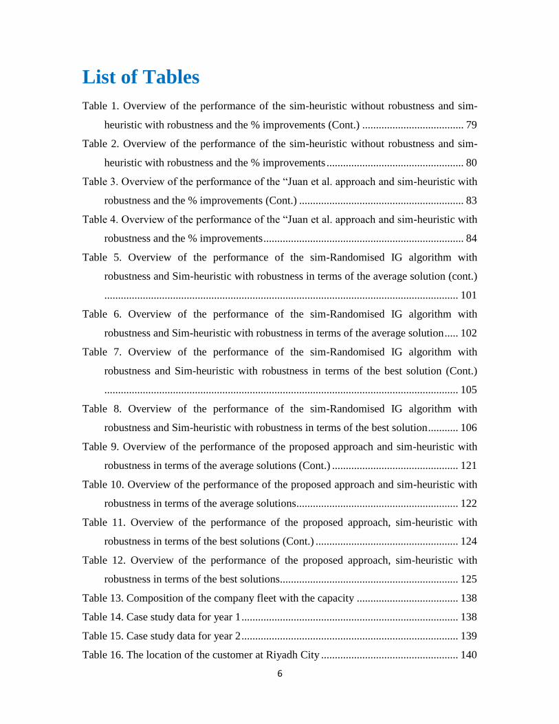
List of Tables

Table 1. Overview of the performance of the sim-heuristic without robustness and sim-

heuristic with robustness and the % improvements (Cont.) ..................................... 79

Table 2. Overview of the performance of the sim-heuristic without robustness and sim-

heuristic with robustness and the % improvements .................................................. 80

Table 3. Overview of the performance of the “Juan et al. approach and sim-heuristic with

robustness and the % improvements (Cont.) ............................................................ 83

Table 4. Overview of the performance of the “Juan et al. approach and sim-heuristic with

robustness and the % improvements ......................................................................... 84

Table 5. Overview of the performance of the sim-Randomised IG algorithm with

robustness and Sim-heuristic with robustness in terms of the average solution (cont.)

................................................................................................................................. 101

Table 6. Overview of the performance of the sim-Randomised IG algorithm with

robustness and Sim-heuristic with robustness in terms of the average solution ..... 102

Table 7. Overview of the performance of the sim-Randomised IG algorithm with

robustness and Sim-heuristic with robustness in terms of the best solution (Cont.)

................................................................................................................................. 105

Table 8. Overview of the performance of the sim-Randomised IG algorithm with

robustness and Sim-heuristic with robustness in terms of the best solution ........... 106

Table 9. Overview of the performance of the proposed approach and sim-heuristic with

robustness in terms of the average solutions (Cont.) .............................................. 121

Table 10. Overview of the performance of the proposed approach and sim-heuristic with

robustness in terms of the average solutions ........................................................... 122

Table 11. Overview of the performance of the proposed approach, sim-heuristic with

robustness in terms of the best solutions (Cont.) .................................................... 124

Table 12. Overview of the performance of the proposed approach, sim-heuristic with

robustness in terms of the best solutions................................................................. 125

Table 13. Composition of the company fleet with the capacity ..................................... 138

Table 14. Case study data for year 1 ............................................................................... 138

Table 15. Case study data for year 2 ............................................................................... 139

Table 16. The location of the customer at Riyadh City .................................................. 140

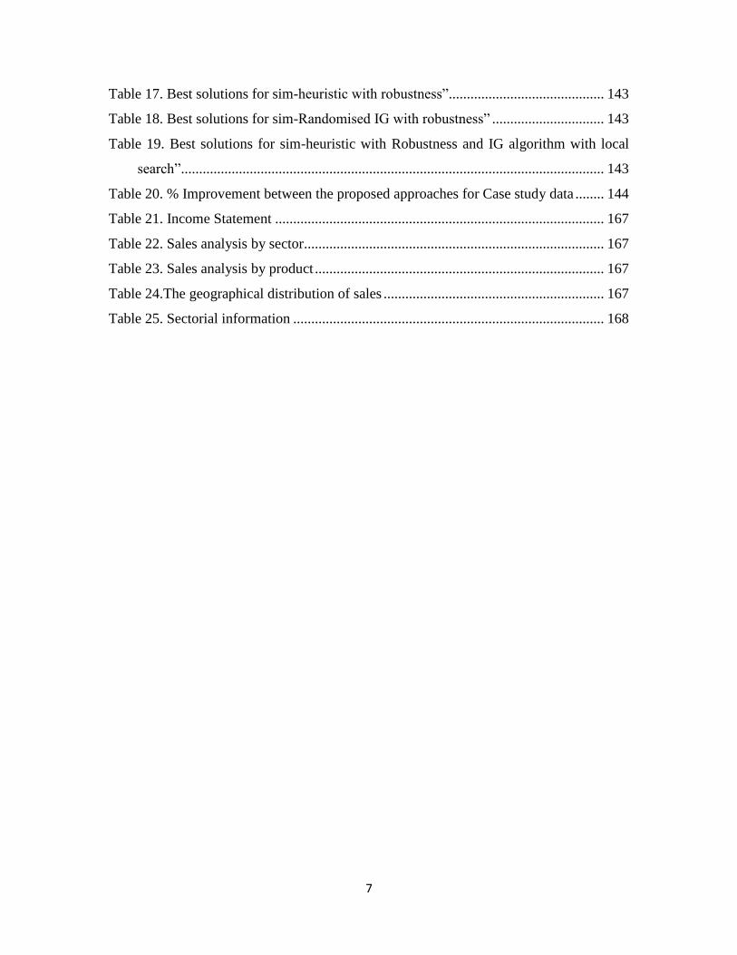
7

Table 17. Best solutions for sim-heuristic with robustness”........................................... 143

Table 18. Best solutions for sim-Randomised IG with robustness” ............................... 143

Table 19. Best solutions for sim-heuristic with Robustness and IG algorithm with local

search”..................................................................................................................... 143

Table 20. % Improvement between the proposed approaches for Case study data ........ 144

Table 21. Income Statement ........................................................................................... 167

Table 22. Sales analysis by sector................................................................................... 167

Table 23. Sales analysis by product ................................................................................ 167

Table 24.The geographical distribution of sales ............................................................. 167

Table 25. Sectorial information ...................................................................................... 168

8

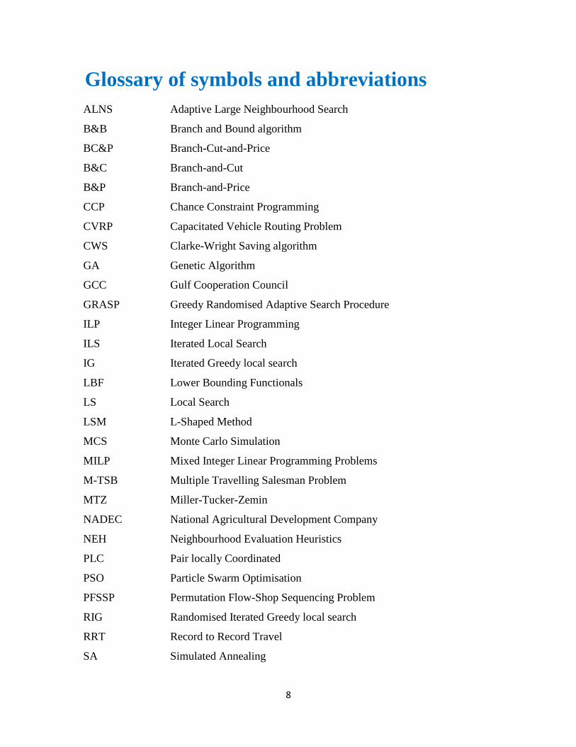
Glossary of symbols and abbreviations

ALNS Adaptive Large Neighbourhood Search

B&B Branch and Bound algorithm

BC&P Branch-Cut-and-Price

B&C Branch-and-Cut

B&P Branch-and-Price

CCP Chance Constraint Programming

CVRP Capacitated Vehicle Routing Problem

CWS Clarke-Wright Saving algorithm

GA Genetic Algorithm

GCC Gulf Cooperation Council

GRASP Greedy Randomised Adaptive Search Procedure

ILP Integer Linear Programming

ILS Iterated Local Search

IG Iterated Greedy local search

LBF Lower Bounding Functionals

LS Local Search

LSM L-Shaped Method

MCS Monte Carlo Simulation

MILP Mixed Integer Linear Programming Problems

M-TSB Multiple Travelling Salesman Problem

MTZ Miller-Tucker-Zemin

NADEC National Agricultural Development Company

NEH Neighbourhood Evaluation Heuristics

PLC Pair locally Coordinated

PSO Particle Swarm Optimisation

PFSSP Permutation Flow-Shop Sequencing Problem

RIG Randomised Iterated Greedy local search

RRT Record to Record Travel

SA Simulated Annealing

9

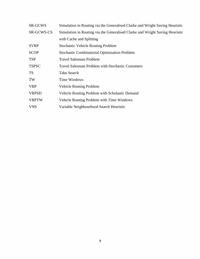
SR-GCWS Simulation in Routing via the Generalised Clarke and Wright Saving Heuristic

SR-GCWS-CS Simulation in Routing via the Generalised Clarke and Wright Saving Heuristic

with Cache and Splitting

SVRP Stochastic Vehicle Routing Problem

SCOP Stochastic Combinatorial Optimisation Problem

TSP Travel Salesman Problem

TSPSC Travel Salesman Problem with Stochastic Customers

TS Tabu Search

TW Time Windows

VRP Vehicle Routing Problem

VRPSD Vehicle Routing Problem with Scholastic Demand

VRPTW Vehicle Routing Problem with Time Windows

VNS Variable Neighbourhood Search Heuristic

10

Declaration

I hereby declare that this thesis has not been submitted, either in the same or different

form, to this or any other university for a degree.

Signature:

11

Acknowledgements

Producing this thesis has been in some ways at least as hard as anything I have previously

attempted, and I certainly would not have reached this point without a great deal of support.

In addition, my research has been a wonderful learning experience. Acknowledgements for

my research and thesis are directed toward many people.

Firstly, I would like to express my heartfelt gratefulness to my thesis advisors Dr. Djamila

Ouelhadj, Dr. Dylan Jones and Dr. Banafsheh Khosravi for their valuable support,

motivation, encouragement, insightful comments, enthusiasm and continuous guidance

during the development of this thesis. They were always open to discussing and clarifying

different concepts and made me feel part of the department. Without their help, this thesis

would not have been possible. I would also like to thank Dr. Angel A. Juan for being the

external advisor of this thesis and for his insightful comments, help and support in the

development of different parts of this work.

My deepest thanks to my family, especially to my wife Mona and my children for their

patience during the long after-work hours necessary to complete this work. Finally, many

thanks to my family back in Saudi Arabia for their support and encouragement, especially

my father and mother for always asking about my work and supporting me.

12

Abstract

The Vehicle Routing Problem with Stochastic Demand (VRPSD) is a fundamental problem

underlying many operational challenges in the field of logistic and supply chain

management. The VRPSD is a well-known NP-hard problem whereby a fleet of vehicles

is located at a single depot. Each vehicle has a limited capacity and has to serve a number

of customers whose actual demands are known only when the vehicle arrives at the

customers’ locations. The VRPSD arises in practice whenever a company faces the

problem of delivering to a set of customers, whose demands are uncertain. The solution to

the VRPSD includes the optimisation of complete routing schedules whilst minimising the

transportation costs (fixed costs and variable costs) to satisfy all the constraints in the

problem. This study proposes three approaches: the robust routing model with sim-

heuristic, randomised Iterated Greedy (IG) algorithm with Monte Carlo Simulation (MCS)

and finally IG algorithm with local search to solve the VRPSD. The main aim of using the

robust routing model with sim-heuristics is to build robust solutions by combining

simulation and optimisation using heuristic methods. This is to handle uncertainty as well

as to optimise against any worst instance that might arise due to data uncertainty. Several

heuristics have been combined with simulation to deal with stochastic demand. In our

version of the approach, the first one is a randomised Clarke and Wright Saving (CWS)

algorithm step after which an MCS is incorporated in order to improve the final solutions

of VRPSD. The second approach proposed the combination of randomised IG algorithm

with MCS to be applied on the VRPSD. The final approach is to use an IG algorithm with

local search, based on the aforementioned first approach, in order to improve the solutions

generated. Local search has been proven to be an effective technique for obtaining good

solutions.

The developed robust routing model and sim-heuristic algorithms are tested on well-known

benchmark instances and a real-life case study is considered in order to evaluate the

effectiveness of the proposed methodologies. The computational results showed that the

proposed methodologies are capable of finding useful solutions for the VRPSD and that

they are good/robust for the stochastic nature of the problem instances. After computing

the average costs from each instance, we also computed the best solution and found that

13

they both could be highly promising and useful for decision makers. The results obtained

are quite competitive when compared to the other algorithms found in the literature.

14

Chapter 1: Introduction

§1.1 Background and motivation

Transportation plays a significant role in our daily lives. Researchers have used different

targets to measure and obtain optimal solutions. The Vehicle Routing Problem (VRP) was

first introduced by (Dantzig and Ramser, 1959). VRP is one of the most significant and

challenging combinatorial optimisation task with clear industry applications. It belongs to

the category of NP-hard problems. The fundamental aim of a VRP algorithm is to optimise

a given objective, i.e. minimising the number of vehicles needed or the total length of

vehicle routes that can be measured in distance (e.g. miles) and travel time (e.g. hours). A

number of specific constraints need to be respected, such as: each vehicle has a limited

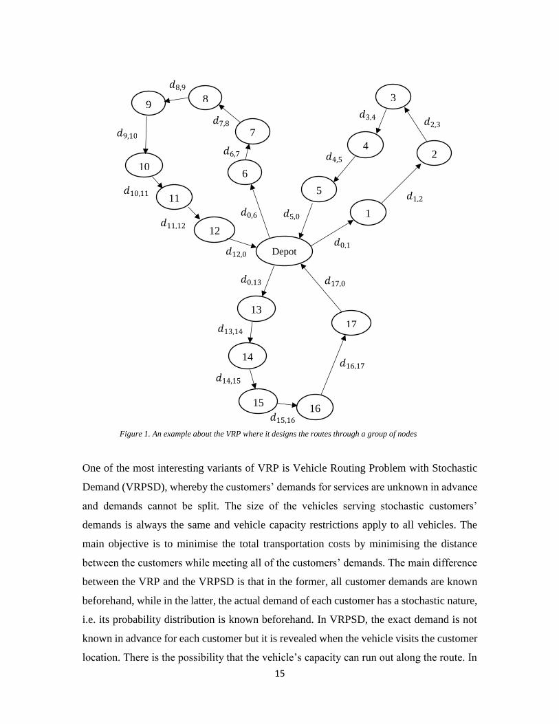
capacity and each customer has a certain demand that has to be satisfied. Figure 1 gives a

good illustration of a VRP and the objective function is to minimise the total travel distance

of the routes generated. In recent decades, extensive research on VRP and associated

scheduling problems has been carried out.

15

One of the most interesting variants of VRP is Vehicle Routing Problem with Stochastic

Demand (VRPSD), whereby the customers’ demands for services are unknown in advance

and demands cannot be split. The size of the vehicles serving stochastic customers’

demands is always the same and vehicle capacity restrictions apply to all vehicles. The

main objective is to minimise the total transportation costs by minimising the distance

between the customers while meeting all of the customers’ demands. The main difference

between the VRP and the VRPSD is that in the former, all customer demands are known

beforehand, while in the latter, the actual demand of each customer has a stochastic nature,

i.e. its probability distribution is known beforehand. In VRPSD, the exact demand is not

known in advance for each customer but it is revealed when the vehicle visits the customer

location. There is the possibility that the vehicle’s capacity can run out along the route. In

𝑑8,9

𝑑7,8

𝑑12,0

𝑑9,10

𝑑10,11

𝑑11,12 𝑑0,6 𝑑5,0

𝑑0,1

𝑑14,15

𝑑0,13 𝑑17,0

𝑑16,17

𝑑15,16

𝑑6,7

𝑑2,3 𝑑3,4

𝑑4,5

Depot

1

5

4

3

2

6

7

8 9

10

11

12

13

14

15 16

17

𝑑1,2

𝑑13,14

Figure 1. An example about the VRP where it designs the routes through a group of nodes

16

this case, the remaining customer demands along the route may not be satisfied. This is

called a failure route (Chepuri, and Homem-De-Mello, 2004). Recourse actions are

considered and each customer on the route receives a unique penalty for not satisfying its

demand. The arc denotes the distance travelled by a vehicle between customers. The cost

for a particular route travelled by the vehicle during a period is calculated as the sum of all

the arcs visited and the penalties (if any) imposed. This includes the arc from the central

depot to the first customer visited and the arc from the last customer visited back to the

central depot. Alternatively, if the vehicle fails to meet the demands of a particular

customer, the vehicle travels back to the central depot at that point terminating the

remaining route. The cost is then the sum of all the arcs visited including the arc from the

customer where the failure occurred back to the central depot and the penalty for that

customer. In addition, the penalties for the remaining customers who were not visited will

also be imposed; thus a given route can have an additional cost associated with it.

Research into VRPSD has focused on improving its practical aspects by setting different

objectives, such as reducing transportation costs or including energy consumption to

protect the environment (Tolga and Laporte, 2011). Other researchers such as Tan et al.

(2007) introduced a multi-objective evolutionary algorithm that combines two VRPSD-

specific heuristics for local exploitation and a route simulation method to estimate the

fitness of solutions. VRPSD can be described as a problem that arises when designing

either optimal collection or delivery routes from a central depot to a set of geographically

dispersed customers. Actual demand is revealed only when the vehicle arrives at the

customer or when setting up a single depot to serve the customers/retailers with a number

of identical or heterogeneous vehicles. A number of mixed fleet vehicles are located in a

central depot and operated by a number of drivers to distribute goods along the most

appropriate road network.

Research on VRPSD has mainly focused on the development of algorithm techniques that

can provide high-quality solutions within acceptable computation times. Numerous exact,

heuristic and metaheuristic algorithms have been proposed by a number of researchers

leading to optimal solutions in terms of cost and/or time. Examples of these algorithms

include the Branch and Cut (B&C) algorithm, the Branch and Bound (B&B) algorithm,

17

Simulated Annealing (SA) algorithm, Tabu Search (TS), Genetic Algorithm (GA), Particle

Swarm Optimisation (PSO) algorithm and Hybrid algorithms. Exact algorithms are able to

solve the problem with a small number of customers, whereas heuristic and metaheuristic

algorithms have the ability to solve the problem for both small, medium and large number

of customers (Bianchi et al., 2004). Heuristics consider methods that can produce better

solutions iteratively. Metaheuristics have been successfully applied to VRPSD and have

also obtained better solutions. Researchers using both heuristics and metaheuristics have

confirmed that a route solution can be improved by adjusting it. For instance, reloading the

vehicle or transferring a customer to another route. Nowadays, researchers propose

combining two different algorithms, e.g., by combining a hybrid VRP algorithm with

parallelisation techniques and simulation to obtain better solutions such as (Juan et al.,

2013). Notice that most real-life applications can use either exact or heuristic or

metaheuristic algorithms to handle hundreds or even thousands of customers.

Other researchers have provided a comprehensive survey of the use of heuristics and

metaheuristics and also their practical applications. Chepuri and Homem-De-Mello, (2004)

proposed a new heuristic method based on the Cross-Entropy method together with Monte

Carlo Sampling to solve the VRPSD. Another aim of their study was the development of

theoretical results to find exact solutions and lower bounds for the VRPSD under various

conditions. This can also serve as a good framework to test other heuristics for the problem

formulation. Properties and formulations of the VRPSD based on a priori optimisation have

also been investigated by Laporte and Louveaux (1992); Bastian and Kan (1992); Trudeau

and Dror, (1992).

In practice, solving the VRPSD in which demand is only revealed when the vehicle reaches

the customer’s location considers one of the competitive goals. Such problems occur in a

number of varieties of real world applications. For example, collecting milk from different

resources/ producers, delivery of home heating oil, delivery of petrol from a big station to

small petrol stations, garbage collection, sludge disposal and distribution of products in

grocery stores. Some applications of VRPSD can be beer distribution to retail outlets,

resupply of baked goods to food stores, replenishment of liquid at research laboratories and

restocking vending machines. Another application of VRPSD is where the daily demand

18

for cash at a bank’s automatic teller machine is uncertain. An obvious application of the

VRPSD is the Dial-and-Ride Problem that has been investigated in many papers e.g.

(Bjerring, 2010) and this problem could be Dial-A-Ride problem for land transport or Dial-

A-Flight problem for air transport.

A robust model aims generally to provide the best feasible solution with all the uncertainty

considered and to optimise against the worst instance that might arise due to this

uncertainty data. In addition, the purpose is to find robust solutions, where routes are

feasible for all customer demand defined by a predetermined uncertainty polytope. The

robust model is able to obtain efficient routing solutions for problems under uncertainty

and to find a feasible solution which satisfies all possible constraint instances. Sungur et

al., (2007) introduced a robust approach in order to achieve a robust solution for the VRP

with demand uncertainty by using an exact algorithm. The approach yielded routes

minimising the sum of the expected values of the total transportation cost and its variability

(the robust term) while satisfying all demands in a given bounded uncertainty set. They

solved the problem directly by using an off-the-shelf mixed integer programming solver.

A novel PSO approach is applied to solve the VRPSD with no known distributions by

Moghaddam et al. (2012). Their proposed model may not be able to satisfy the demand

fully but it incurs less cost. Also in all cases, the proposed method has achieved a feasible

solution while the other methods, in many cases, have not achieved any feasible solutions.

In conclusion, the robust approach provides the solution while satisfying all demand

outcomes from the uncertainty set and have the potential to be viable solutions in practice.

Recently, sim-optimisation has been suggested as a new research area to deal with

uncertainty. In general, this is a simulation-optimisation (SimOpt) approach with the

simulation as an evaluation function of the optimisation algorithm. This is a promising

approach and its application area includes transportation and logistics. A number of studies

have combined simulation and optimisation approaches to improve solutions and to deal

with realistic-complex scenarios. Therefore, the combination of complementary techniques

is quite popular in the research community. The sim-heuristic approach is a particular case

of simulation-optimisation which combines a heuristic/metaheuristic algorithm with

simulation methodologies. For example, MCS, discrete-event and agent-based simulation

19

in order to efficiently deal with the two components of a Stochastic Combinatorial

Optimisation Problem (SCOP): the optimisation nature of the problem and its stochastic

nature. For instance, Juan et al., (2011b) combined MCS with routing metaheuristics in

order to solve the VRPSD. Juan et al., (2013c) reviewed the related literature and provides

an example of simulation-optimisation methods. One of the main contribution of (Juan et

al., 2013c) was the description of an efficient and flexible methodology that combines MCS

and parallel-computing to achieve real-time solutions to the VRPSD. Also, their aim was

to find minimum-cost routes between two customers, so that both the required time to serve

all customer’s demand locations and the sum of waiting times were minimised.

From the literature, it is clear that very few researchers have considered a robust model in

order to provide solutions to VRPSD. Whereas, no research has combined robust routing

model with sim-optimisation to deal with uncertainty. Most VRPSD studies are conducted

on stochastic customer demand with a cost minimisation objective function. However, the

solution methods for VRPSD is very diverse, including exact methods, heuristics and

metaheuristics techniques. This research is the first of its kind in the field of VRPSD. Based

on a systematic review of the VRPSD literature and conducted survey, we proposed to

address the research gap by developing a robust routing model suitable for solving VRPSD

combined with an efficient approach such as sim-heuristic. Also, we addressed the research

gap by integrating MCS inside randomised IG algorithm with robustness, in order to

improve solutions for VRPSD generated by a CWS heuristic. In addition, we addressed the

VRPSD without considering safety stock by developing an IG algorithm with local search

in an effort to improve the solutions of VRPSD. The main aim is to provide efficient

support to decision-making in the VRPSD using these three contributions. As a result, these

contributions have the potential to be interesting, not only for the academic community but

also for real-life problems and the business sector. Hence, in this research, we applied the

developed model and the proposed approaches to a real world case study based on real data

collected from NADEC Company in the kingdom of Saudi Arabia (KSA).

20

§1.2 Aims and objectives

This study addresses VRPSD. The research study focuses on offering better routing

decisions in order to minimise the expected total transportation costs. The problem

presented in this thesis is inspired by real-life applications with the hope that practitioners

will be able to use the methods explained in this study. In the VRPSD, the exact demand

of each customer has a stochastic nature and it is revealed only when the vehicle arrives at

the customer’s location. One common practice to handle uncertainty in customer demands

is that the vehicle routes are designed in advance by applying a specific algorithm.

However, due to the uncertainty of customer demand, at some point along a route the

vehicle capacity may be depleted before all customer demands on the route have been

satisfied. Therefore, some corrective or recourse actions are required in the event of such

an occurrence.

In general, a desirable or efficient optimisation algorithm with simulation to solve VRPSD

should produce good or high-quality solutions, be simple to configure, flexible to be

adapted to new constraints and easy to understand and implement (Cordeauet al., 2002).

The overall aim of the research is to improve on the existing current solution methods for

VRPSD. This improvement can be obtained by applying the following:

Develop, implement and test a robust routing model with sim-heuristic to solve the

VRPSD. Sim-heuristic will combine biased randomised CWS with MCS.

Evaluate the performance of the algorithm under uncertain scenarios. For this, we

propose an algorithm which combines a randomised IG algorithm with MCS and

robustness to find near-optimal solution for VRPSD.

Improve the quality of the solutions, by implementing IG algorithm with local

search. This, in turn, will contribute to significant improvements in the quality of

VRPSD instances solutions.

Promote knowledge transfer to real-life problems, in order to improve the

competitiveness of the company by using the robust routing model with these

approaches when designing the distribution plan.

In order to accomplish these aims, several steps must be achieved. First of all, sim-heuristic

21

is designed and implemented with the robust routing model to solve VRPSD instances.

This sim-heuristic methodology is based on heuristics, biased randomisation and

simulation in order to efficiently support decision-making processes in the VRPSD area.

Secondly, the application of the methodology to the problem at a higher level is presented

before introducing the pseudo-code for the proposed algorithm. Then, the algorithm is

implemented on benchmark problems extracted from the literature. After that, the results

obtained by the model with the proposed algorithm are analysed in terms of the

minimisation of expected total cost. This enables us to compare the quality of the algorithm

results with the results reported in the literature.

Regarding the benchmark problem, there are some issues that could be found when a

VRPSD is developed, e.g. not having data to execute tests. Various studies used real data

provided by companies even though the data used was private or sometimes difficult to

access. Some studies generated instances following random aspects or specific probability

distribution. In our study, we used both cases: firstly, we used several well-known instances

to test the developed model and proposed approaches, each of these instances have been

developed for a specific VRP branch. Secondly, real-life data from NADEC Company was

used for testing the performance of the developed model with proposed approaches.

22

§1.3 Contributions

In the process of achieving the objectives described in the previous section, a series of

original contributions to the existing research are made. The most relevant ones are

summarised as below and are explained in detail in the study.

1. The robust routing model with sim-heuristic for solving VRPSD: The robust

routing model is proposed to develop robust solutions to the problem with the aim

of minimising the expected total cost in the presence of uncertainty. The robust

routing model can produce good solutions for VRPSD compared to other solutions

and the robust framework can be very useful when the information of the

customer’s demand is not available. A second objective is centred around the

combination of randomised heuristic with simulation (Sim-heuristic) to be applied

on the VRPSD. The sim-heuristic approach is based on the randomised CWS

heuristic with MCS for the VRPSD. This combination has the characteristic of

obtaining good results, which makes it suitable to use with the robust routing model

to achieve an optimal solution of VRPSD. The experimental results showed the

potential of the proposed model with sim-heuristic in terms of the quality of the

solution as it is able to obtain robust solutions for the problem. Our model

demonstrates a better performance when combined with sim-heuristic.

2. The Sim-Randomised IG heuristic for solving VRPSD: To our knowledge, this

algorithm has not been used in the literature to solve VRPSD. IG algorithm has

been shown to be very successful for solving a considerable number of different

Combinatorial Optimisation Problems. For example, IG algorithm has been applied

successfully for the Permutation Flow Shop Scheduling Problem (PFSSP) (Ruiz

and Stützle., 2007). For this, we adapted this algorithm to solve the VRPSD. In

order to achieve this aim, we first proposed the IG algorithm to handle the

deterministic case. This algorithm is then developed and extended to deal with the

stochastic case where the robust routing model is used with a sim-randomised IG

algorithm; this was to improve the solution for the VRPSD for the first time in the

23

literature. To validate the proposed algorithm, computational experiments are

conducted on a benchmark set from the literature. From the perspective of

experimental results, this algorithm is easy to implement as it has no parameters.

Also, the model with the approach showed the effectiveness needed in order to

improve the solutions of the algorithm in most of the instances.

3. Robust routing model and sim-heuristic with IG algorithm and local search

for the VRPSD: To solve the VRPSD, the IG algorithm with a local search is

proposed to improve the final solutions obtained using the aforementioned model

and approach described in chapter 3. We started off using the robust routing model

with sim-heuristic then implemented IG algorithm with local search. Applying the

IG algorithm with local search provides excellent results and has improved the best-

known solutions to benchmark problems. In terms of the computational results, we

have adapted the IG algorithm with local search for the customer demand variation

of the VRP and evaluated its performance. The IG algorithm with local search

results showed that it is able to outperform the two aforementioned methodologies

described earlier in most or all of the instances considered. With that, we

demonstrated the potential of local search to facilitate the discovery of high quality

solutions by embedding them within the IG algorithm framework to solve the

VRPSD.

4. Application to case study problem from National Agricultural Development

Company (NADEC): Nowadays, urban transportation is a strategic domain for

distribution companies. In academic literature, this problem is categorised as a

VRPSD. This is a popular research stream that has undergone significant theoretical

advances, but has remained far from practical implementation. To promote the

knowledge transfer to a real-life problem, we can implement data of the company

by using the robust routing model with the proposed approaches when designing

the distribution plan. The aim of the case study was to show the efficiency of our

model and proposed approaches. We focused on VRPSD faced by a Saudi food

distribution company (NADEC) on a daily basis in order to reduce the expected

24

total transportation costs. In this study, we considered a routing problem with a

number of vehicles, limited capacity, customer’s demands and the location of each

customer. Different algorithms with the robust routing model developed earlier will

be implemented and compared. We executed our algorithms and model with data

from a company that distributes prepared food in Riyadh. In terms of computational

experiments, the results reveal promising improvements in the different

approaches.

25

§1.4 Structure of thesis

This thesis studies VRPSD, designing algorithms for VRPSD based on Sim-heuristics

frameworks, and developing the robust routing model for solving VRPSD. To this end, the

thesis is structured including the following chapters:

Chapter 2 presents an overview of Vehicle Routing Problem with Stochastic

Demand. A review of both robust routing model and the sim-heuristic method to

solve the Vehicle Routing Problem with Stochastic Demand is presented. In

addition, the use of varios methodologies applied on Vehicle Routing Problem with

Stochastic Demand to optimise different objective measurements are explained.

This includes exact methods and heuristic approaches in order to solve different

benchmark problems. Sim-heuristic is based on the use of biased randomisation

with simulation for solving complex optimisation problems. This method has been

proven to be useful for solving routing, scheduling and availability problems,

especially in the field of transportation and logistics. In this thesis, we aim to adapt

these algorithms and apply them on VRPSD with a robust model.

Chapter 3 introduces the main part of the thesis, which is the robust model with

sim-heuristic, in order to deal with stochastic variables in the resolution of VRP

scenarios (VRPSD) using simple simulation techniques. Solutions for the VRP

cases with stochastic demands are provided.

Chapter 4 is divided into two parts. The first part proposes a novel heuristic that

has not been implemented on VRP before in literature. This novel heuristic is an

IG algorithm and deals with deterministic cases. The second part extends the

deterministic case to a stochastic case by proposing a Randomised IG algorithm

with MCS for solving VRPSD.

Chapter 5 proposes an IG algorithm with local search to improve the final solution

of the robust model with sim-heuristic. An IG algorithm with local search is applied

after using the sim-heuristic with a robust model for solving VRPSD.

Chapter 6 presents a case study. An attempt was made to test all the mentioned

approaches by using a real-life case study in Saudi Arabia (Riyadh) and comparing

the computational results.

26

Chapter 7 summarises the main achievements of the study, presents the general

conclusions, and proposes possible areas for further research.

In all chapters, the adaptation of some heuristics to solve the VRPSD and constraints is

considered. This study examines how the solutions to the VRPSD could be improved by

integrating a robust model with heuristics, simulation, and biased randomisation. These

integrations can help to design effective methods to solve VRPSD. These methodologies

are tested with well-known benchmark problems available in the literature and the results

are compared to those from other studies.

§1.5 Chapter summary

We enumerated the main contributions of this study which will be introduced in more detail

in the following chapters. A brief explanation of the structure of the study is presented in

terms of giving a clear picture about the whole thesis. The following chapters describe the

various aspects of this study, such as literature review, definitions, models, problem

description, the description of competitive algorithms to solve the VRPSD, computational

results on well-known VRPSD benchmarks and conclusions.

27

Chapter 2 : Literature review of VRPSD

§2.1 Introduction

Stochastic Vehicle Routing Problem (SVRP) has an obvious difference from deterministic

VRP because some important properties of the latter are no longer held in the former. In

the deterministic problem, decision-makers have all the information when generating

vehicle routes and the routes do not change once they are in execution. In the stochastic

problem, all input is unknown when the decision-maker wants to generate the routes;

however probabilistic information about the future may be known. Due to the number of

variables and side constraints considered, research in the areas of SVRP is growing both

intensively and extensively at a rapid pace. Some of the basic objectives of the SVRP are

to minimise the transportation cost or numbers of vehicles in the fleet, or minimise the

routing travel time. Berhan et al. (2014a) developed a structural classification of SVRP

using different domains and attributes. The aim of this study was to help summarise and

map a comprehensive survey of SVRP literature.

Oyola et al. (2016) have reviewed the past 20 years of scientific research on SVRP and

also described and categorised many variants of the SVRP that have been considered. They

also presented a number of approaches that have been proposed to deal with different

variants of the SVRP. Uncertainty can emerge in different aspects of VRP. Uncertainty

may affect any of the input data and the most common examples of the uncertainty in VRP

are as follows: uncertainty linked with the demand - called VRP with Stochastic Demand

(VRPSD) and uncertainty linked with the customer - called VRP with Stochastic

Customers (VRPSC). In addition, uncertainty may concern the time, such as VRP with

Stochastic Travel Time (VRPSTT) and VRP with Stochastic Service Time (VRPSST). The

uncertainty may also be linked with two variants, such as VRP with Stochastic Demand

and Customers (VRPSDC).

Sometimes, the customer demands, travel and service times, and the presence of customers

are modelled stochastically (Gendreau et al. 1996a; Tan et al. 2007). An early literature

review in the VRPSD with other variants in (Gendreau et al., 1996a) included a brief

28

description related to solution concepts and algorithms. Two stages can be used to solve a

VRPSD; a first stage is computed, the realisations of the random variables are then

disclosed and, in a second stage, a corrective action can be taken when the values of the

random variables are known. This is a feature of many real life problems such as the one

studied by Yang et al. (2000). However, for VRPSD, the decision-makers have to make a

decision for the solution (at least partially) with partial information. In some situations,

some constraints can be violated. For example, the total real customer demands on a

planned route may actually exceed the capacity of the vehicle. Because some of the

information is random, it is no longer required to satisfy the constraints for all realisations

of the random variables, and new feasibility and optimality concepts are required. With

respect to their deterministic counterparts, SVRPs are considerably more difficult to solve

(Cordeau et al., 2007). Therefore, the most studied version of SVRP is the VRPSD where

customer demands are random and usually independent. Gendreau et al. (2014) provided a

tutorial with a synthesis of some recent literature in the VRPSD with other variants.

In terms of the robust model, little research has been presented. The purpose of using a

robust model is to obtain efficient routing solutions for VRPSD. The robust model is an

attractive alternative for formulating routing problems under demand uncertainty as it does

not require distribution assumptions on the uncertainty (Sungur et al., 2007). Sungur et al.

(2007) proposed the Miller-Tucker-Zemlin formulation (MTZ) of the Capacitated Vehicle

Routing Problem (CVRP) in order to minimises the total cost distance of the problem. Also,

they proposed several constraints such as vehicles leaving and returning to the depot, each

vehicle visits each customer exactly once and the vehicle capacity should not be violated.

They presented computational results on instances from the literature and analysed the

trade-offs of robust solutions on families of clustered instances. They also compared the

robust solution with alternative methods to address VRPSD.

Several studies have combined simulation and optimisation approaches in order to

minimise a different number of objectives such as time or total route cost. In addition,

simulation and optimisation are able to provide solutions to practical and complex real-life

problems. Recent advances indicated that simulation and optimisation technology is able

to solve problems more effectively, specifically in applications involving risk and

29

uncertainty. Several studies have been conducted on this matter for different purposes

(Glover et al., 1996, 1999). In the last few years, the integration of simulation with

optimisation has undergone remarkable changes by making simulation applications

available that had previously been considered infeasible or beyond the scope of current

technology to handle. In addition, the timescale has been reduced in terms of finding near-

optimal solutions. A number of applications have used simulation-based optimisation to

deal with realistic complex scenarios. This chapter is organised as follows. In section 2.2,

we reviewed the related literature of VRPSD. In section 2.3, we gave an overview of the

related literature of robust model routing. We included some of the most important solution

methods that are related to solve the VRPSD in section 2.4. In section 2.5, we presented an

overview of the related papers of sim-heuristic with benefits of using sim-heuristics. We

summarised the chapter in section 2.6.

§2.2 Vehicle Routing Problem with Stochastic Demand (VRPSD)

The VRPSD is a well-known NP-hard problem (Bastian and Rinnooy 1992) in which a

number of customers with unknown demands are to be served by a fleet of homogeneous

vehicles departing from a depot and returning to the depot, which initially holds all

available resources. The costs are often related to the total distance travelled from the depot

to the customers and from one customer to another. These costs are usually assumed to be

symmetric. Also other factors e.g. number of vehicles employed, or service times for each

customer, can be included. The central point of the VRPSD is that the actual demand of

each customer has a stochastic nature that follow a well-known theoretical or empirical

probability distribution, either discrete or continuous, with a known mean. Before reaching

the customer locations, the distribution of the customer’s demands are known. Upon

arrival, customer demands are observed and served to the maximum extent, given the

available vehicle capacity. When its capacity is exceeded, a vehicle has to apply recourse

actions. Therefore, VRPSD is a more complex problem due to the uncertainty introduced

by the random behaviour of customer’s demands. The standard aim is to find the feasible

solution that minimises the expected total costs subject to the following constraints: (i) all

30

vehicle routes begin and end at the central depot; (ii) each vehicle has a maximum load

capacity, which is considered to be the same for all vehicles; (iii) all (stochastic) customer

demands have to be satisfied; (iv) each customer is supplied by a single vehicle; and (v) a

vehicle cannot stop twice at the same customer without incurring a penalty cost. In

addition, a number of different constraints and factors are sometimes considered to solve

VRPSD such as number of vehicles, number of depots, maximum allowable costs for a

route, costs associated with each demand, environmental costs, loading splitting

constraints, time windows for serving each customer and other externalities.

In VRPSD, the customer demands are stochastic and become known only when the vehicle

arrives at the customer locations. The routes are designed before the customer demand

becomes known to the decision-maker. Furthermore, each vehicle has a limited capacity

from a depot to serve a number of geographically dispersed customers. The customers’

demands are usually independent in this problem. The VRPSD can be described as a

problem that a number of the vehicles located in the central depot are ready to serve

different varieties of the customer's demands in different locations (Tillman, 1969).

Tillman (1969) was the first to present an algorithm that is based on the Clarke and Wright

Saving (CWS) algorithm (Clarke and Wright, 1964) for solving the VRPSD, in a case

where there is a number of depots. Penalties are incurred whenever a vehicle is filled over

capacity. An early study on VRPSD is that of (Stewart and Golden, 1983), who used several

formulations including a chance constrained model, two other models, and to apply

heuristic algorithms to solve the VRPSD. The first model used a penalty proportional to

the probability of exceeding the capacity of the vehicle. The second model related to the

expected demand, thus the penalty is proportional to the expected demand which is in

excess of the capacity of the vehicle. Two algorithms are implemented: One based on the

CWS algorithm and another based on Lagrangean relaxation, considering some demand

distributions. Notice that (Tillman, 1969; Stewart et al. 1983; Dror and Trudeau., 1986)

proposed different modification to saving the algorithm of CWS.

As the authors proposed, CWS used for generating an a-priori solution for the problem.

Later, Dror and Trudeau (1986) presented a modification of the CWS algorithm when the

real customer demand is not revealed with certainty and vehicle routes are designed. Also,

31

the authors showed that the expected travel cost depends on the direction of a designed

route. Bertsimas (1991) proposed a heuristic with different recourse policies to deal with

the VRPSD and suggested several bounds, asymptotic results and analysis of the VRPSD

using a variety of theoretical approaches. The aim of the recourse policies is to describe

what actions to take in order to repair the solution after a failure. Most of the literature

studied the a-priori solution approach, based on CWS algorithm. The goal of Secomandi.,

(2001) work was to develop a computationally tractable heuristic for computing a

reoptimisation-type routing policy. This has been accomplished by sequentially improving

a given a-priori solution by a rollout algorithm. After describing the solution strategy and

providing properties of the rollout policy, the policy behaviour is analysed by conducting

a computational investigation. Depending on the quality of the initial solution based on

CWS, the rollout policy obtained 1% to 4% average improvements on the a-priori

approach, within a reasonable computational effort. The CWS heuristic is based on the

simple premise of iteratively combining routes in order of those pairs that provide the

largest saving.

Recourse policies are allowed to adjust an a-priori solution after the uncertainty is revealed.

As Sungur et al. (2007); Tan et al., (2007) proposed three common policies to obtain near-

optimal solutions for VRPSD. The first recourse is to send the vehicle back to the depot

for restocking when the vehicle capacity is exceeded. Second policy, which is preventive

restocking, can help to reduce the cost of travelling back to the depot from the failed

customer location. This policy can also be done before a route failure occurs. The last

common policy is to re-optimise the part of the route with a number of customer’s demands

that have not been served, after the route failure has occurred and the customer demand has

become known. The decision-maker can also decide which customer has to be visited next,

either on the route incorporating replenishment at the depot or as part of the regular routing.

Tan et al. (2007) considered VRPSD with a limited capacity and time windows constraint.

They have introduced a multi-objective evolutionary algorithm to solve a multi-objective

and multi-modal optimisation problem. Multi-objective incorporated two VRPSD specific

heuristics for local exploitation and a route simulation method to evaluate the suitability of

the results. Their solution to the VRPSD involved the optimisation of complete routes for

multiple vehicles with minimum travel distance, the optimisation of driver remuneration

32

and the number of required vehicles. In terms of time-constrained VRP with stochastic

demand, a possible recourse policy is to apply a penalty when the duration of a route

exceeds a given bound. Also, this kind of penalty can correspond to the overtime pay that

a driver receives.

Juan et al. (2011a) and Marinakis et al. (2013) studied the random behaviour of customer’s

demands that could make the feasible solution become infeasible, in a case where the final

demand of any route exceeds the origin vehicle’s capacity. They referred this case as route

failure and the decision makers should try to resolve this by introducing corrective actions

in order to achieve a feasible solution. For some recourse actions, a decision maker can

consider a safety stock in each vehicle during the execution. Also, a vehicle may travel

back to the depot after route failure to reload and resume distribution at the last visited

customer. Juan et al. (2011a) defined the VRPSD as an NP-hard problem in which a set of

customers with stochastic demands has to be served by a homogeneous fleet departing from

a single central depot that initially holds all available resources. They assigned different

levels of safety stocks that the routed vehicles must employ to deal with unexpected

demands, and they consider a vehicle capacity lower than the actual maximum capacity

when designing the VRPSD solutions. They used the MCS to achieve estimates of the

reliability of each a-prioristic solution. In addition, the expected costs are linked with

recourse actions gradually, after a vehicle capacity is exceeded and before completing its

route. Juan et al. (2011a) aim to reduce the probability of occurrence of such undesirable

situations to a reasonable value, which is defined as a utility function – according to the

decision-makers. Moreover, they attempted to avoid route failure by keeping a safety stock

in each vehicle for emergencies. The goal of using safety stock is to cover route failures

without having to assume the usual high expected costs involved in vehicle restocking trips.

Juan et al. (2013) focused on solving the VRPSD and explain the combination of the

Parallel CWS and MCS to efficiently solve the VRPSD. Also, their algorithm solved each

scenario by integrating MCS embedded in a randomised heuristic process. They considered

different levels of safety stocks when they deal with uncertainty in the customer demands

in order to offer a flexible as well as an efficient algorithm for solving the VRPSD. They

have obtained good solutions for VRPSD but the study does not consider the robust model

during the implementation.

33

Marinakis et al. (2013) suggested that the vehicles leave the central depot with a full load

to serve several customers whose demands are known only when the vehicle arrives to

customers’ locations. They investigated a hybrid algorithm that is based on a combination

of the PSO to solve the VRPSD. The finite vehicle capacity and two simple local search

metaheuristics and the Path Relinking strategy can be combined in a hybrid scheme in order

to give very good results for the VRPSD. In PSO algorithm procedure, initially a number

of particles is created randomly where each particle corresponds to a potential solution.

Each particle has a position in the space of solutions and moves with a given velocity. One

of the main issues in designing a successful PSO for the VRPSD is to obtain a suitable

mapping between particles in PSO and VRPSD. In a study by Marinakis et al. (2013), the

objective function included the expected cost of the route when a vehicle does not travel

back to the central depot but continues to serve the next customer, and also includes the

expected cost when the vehicle travels back to the central depot for preventive restocking.

The way they dealt with route failure is given in the following: when the route failure

occurs, the vehicle is sent to the depot, then, it returns to the customer location where the

route failure occurs and continues the service. The second way is a preventive restocking

strategy such as using safety stock in order to serve the rest of the customers.

Novoa and Storer (2009) developed efficient and flexible rollout algorithms in order to

solve the VRPSD. The rollout algorithms have a type of policy iteration where single or

multiple initial suboptimal base policies are sequentially improved. These algorithms

should be efficient because it has the ability to provide an optimal or near-optimal solution

to both small and medium VRPSD instances within reasonable computing time. In terms

of the flexibility, no further assumptions need to be made concerning the random variables

which are used to model customer demands, e.g. these variables should not be assumed to

be discrete or follow any particular distribution. According to C´aceres-Cruz (2013), most

of the existing approaches in the literature solve the VRPSD but do not satisfy the

efficiency and flexibility requirements. Therefore, one of the most important contributions

of the study by C´aceres-Cruz (2013) was the application of an efficient and flexible

methodology that combines MCS and parallel-computing, to obtain real-time solutions to

the VRPSD. The aim was to minimise the total expected cost, which consists of fixed costs,

34

expected variable costs and a trade-off between two costs. Also, authors explained how a

multiple scenario approach based on the safety stocks level works in a good way as well

as the range of safety stocks which have been used, between 0% to 20% of the capacity of

each vehicle.

Several researchers have applied a different model with approaches to solve the VRPSD,

such as (Chang, 2005) proposed a nonlinear stochastic integer programming with recourse

to formulate the VRPSD. An optimisation algorithm is developed by applying the L-shaped

method. In addition, this approach was able to minimise the total cost of the first stage

solution and expected recourse costs. The first stage contained the total cost between

customers and total waiting cost at all customers’ locations. The expected recourse costs

contained the cost incurred in order to finish the routes which were planned in advance.

Noorizadegan et al. (2012) use a basic Miller-Tucker-Zemin (MTZ) formulation and

proposed branch-and-cut algorithms to solve the Heterogeneous Vehicle Routing Problem

under demand uncertainty. This paper discussed Heterogeneous Vehicle Routing Problem

under demand uncertainty with unlimited number of the vehicles, and the multi-depot

Heterogeneous Vehicle Routing Problem under demand uncertainty with limited number

of vehicles. Noorlzadegan et al. (2012) compared the deterministic, robust optimisation

and exact algorithm that are based on different performance measures such as extra cost,

unmet demand and recourse cost. Sun and Wang (2015) considered failure and successful

scenario. They formulated a solution procedure for VRP with uncertainty with regard to

two factors: future demand and transportation cost. Also, they proposed Expectation

Semideviation Robust Optimisation Approach (E-SDROA) for solving the VRP with

uncertainty. Their contribution was to focus on the robust optimisation formulation for this

problem, to minimise the total expected cost. As a result, their approach has the ability to

deal with some cases involving bidding or capital budget decisions. The result of (E-

SDROA) approach showed a trade-off between the expected value of the total cost in all

failure scenarios and its variation and successful scenarios. Moreover, both the similarities

and differences of the robust optimisation model and existing robust optimisation

approaches are compared.

35

The quality of the solutions is assessed using a new proposed way of comparing the

expected costs. Therefore, Bianchi et al. (2004) analysed the performance of number of

metaheuristics for the VRPSD. They investigated two types of hybridisation of

metaheuristics by means of two objective functions. Also, two different approximation

schemes for evaluating the expected distance cost of a local search move, are considered.

The main contribution of the study by Bianchi et al. (2004) is to test the impact of using

the length of the a-priori tour on the metaheuristics’ performance, as this can be a fast

approximation of the exact, but computationally demanding, objective function. In terms

of experimental comparisons of (Bianchi et al., 2004), the computational result showed

that metaheuristics achieved better solutions with respect to the cyclic heuristic, which is

known from the literature to achieve good results on different types of benchmarks

problems. Bianchi et al. (2006) investigated the use of objective function approximations

derived from deterministic problems in the context of VRPSD. They improved the

computational result one step further and their metaheuristics found better solutions with

respect to both the cyclic heuristic and with respect to solving the travelling salesman

problem. To conclude Bianchi et al. (2004, 2006) have applied a simple SA algorithm to

the VRPSD and implemented several metaheuristics, namely, Ant Colony Optimisation,

Evolutionary Computation, TS and Iterated Local Search.

A number of researchers provided a complete background with unified view of

metaheuristics that lead researchers to design, understand and implement metaheuristics to

solve VRPSD. A number of problems are solved by metaheuristics as can be seen in

logistics and transportation, scheduling and telecommunication applications. Ismail and

Irhamah (2008) proposed a hybrid GA with TS heuristic under a-priori approach, with

preventive restocking during route design. Their method solves a single VRPSD where the

customer demands are random variables with a known probability distribution. In addition,

they conducted a comparative study between their approach which is GA and TS

approaches for solving the VRPSD. The data is inspired by a real case study of VRPSD in

a waste collection problem. The computational results of the waste collection data showed

the advantages of the proposed algorithm in terms of solution quality. A set of very well-

known metaheuristics methods, widely used in literature, in order to solve the VRPSD, are

presented by Bianchi et al. (2009) and Hemmelmayr et al. (2010). They have surveyed a

36

number of metaheuristics to solve varied classes of combinatorial optimisation problems

with demand uncertainty. These metaheuristics are emerging as effective alternatives for

solving VRPSD and other optimisation problems. One of the advantages of these articles

is that they have provided enormous references regarding the use of metaheuristics in

VRPSD and other related problems. In addition, they proposed some possible directions of

research with guidelines. The main contribution in these articles is to summarise the

achievements in theoretical proofs of convergence which can help researchers to find a gap

for new investigations. Moghaddam et al. (2012) investigated VRPSD by implementing an

advance PSO algorithm. They also developed the decoding scheme to increase the PSO

efficiency. They assumed customer’s demands are uncertain and with not enough detail

available to estimate the probability distribution of uncertain parameter values.

Subsequently, they analysed the solution by considering the trade-offs between exact

robust solutions in (Sungur et al., 2007) and the proposed heuristic method. Finally, they

proved that the exact robust method meets all uncertain demands while their method has

some unmet demands.

Balaprakash (2015) suggested some estimation-based metaheuristics for solving the single

Vehicle Routing Problem with Stochastic Demands and Customers. They customised the

estimation-based procedure to evaluate the final solution cost of the VRPSD. The methods

are implemented on four instance sizes and the same probability value is assigned to all

customers except the central depot. They considered probability values between 0.05 and

0.2 and showed the current best algorithm for solving VRPSD. Mendoza et al. (2015)

proposed a hybrid metaheuristic including a Greedy Randomised Adaptive Search

Procedure (GRASP) with a heuristic to solve route-duration constraints in the VRPSD.

They have tested this methodology on 40 instances for classical VRPSD. The Variable

Neighbourhood Search Heuristic (VNS) approach is used to solve VRPSD under a

preventive restocking policy and to obtain a minimum expected tour length in the study by

Biesinger et al. (2015). Furthermore, two different algorithms have been applied to find an

initial solution and three types of well-known neighbourhood structures are used in the

VNS part. After examining these methods, the outcomes showed that their methodology is

able to address larger instances and the VNS approach is able to provide an optimal or

37

near-optimal solution in much shorter time. On top of that a multi-level evaluation scheme

was used in order to substantially reduce the time needed for evaluating a solution.

The idea of Paired Locally Coordinated (PLC) has been developed in the study by (Zhu et

al., 2014) as part of a Paired Cooperative Re-optimisation (PCR) strategy for the VRPSD.

This strategy is proposed to be used between a pair of vehicles. The major contribution was

to use a bi-level Markov decision process (MDP) to develop the PCR recourse strategy.

This kind of strategy allowed a pair of vehicles to dynamically visit a number of customers

under a re-optimisation policy. The vehicles run independently until the information is

shared, which occurs after any of the vehicles finishes visiting its assigned customers’

demands. The process of solving VRPSD started dividing the customers into two clusters

and assigned a cluster to each vehicle. When one vehicle has finished its assignment, the

remaining customers who have not been visited yet by the second vehicle are divided into

two clusters and assigned to each vehicle. Both vehicles are able to communicate and

dynamically modify their routes in order to visit all customers’ demands. This process is

repeated until all customers in the problem are visited. The sequence of the visits in each

group is determined by partial re-optimisation. In this problem, Zhu et al. (2014) followed

a uniform discrete probability distribution for the customer demand. The model considered

three assumptions: firstly, the customer service time is ignored, the travelling speed of

vehicles has to be the same, and finally, vehicles do not have any idle time. The PCR

reduced the cost when it is compared with the PLC which showed that the use of

communication helped to reduce the cost.

§2.3 Robust routing model

Robust optimisation based on the definition of model robustness (Mulvey et al., 1995): this

approach mainly focused on the feasibility of the optimal solution from a set of scenarios.

They have achieved several aims: firstly, they developed a general framework for

achieving robustness and secondly, they discussed the relative merits of robust

optimisation over sensitivity analysis and stochastic programming. Finally, they also have

seen how robust optimisation models would indeed generate robust solutions for some

38

applications. Only a few studies applying robust routing to the VRPSD have been

published. The robust routing is considered as a particular case of robust optimisation. The

main approach of a robust routing model is to achieve a solution against the worst scenarios

that might arise due to the uncertainty of data (e.g. customer presence, demand

requirements, travel or service times). The uncertain parameters in the robust routing are

described by discrete scenarios or a continuous range. In addition, the robust solution can

prevent having unsatisfied demand by increasing a small cost. The robust model can

carefully deal with the remaining vehicle capacity cover all demands with minimum cost.

A number of robust model formulations have been presented in different articles such as

(Sungur et al., 2007).

Sungur et al. (2007) presented an MTZ formulation for solving demand uncertainty sets.

Their robust model approach for the VRPSD used the remaining vehicle capacity and made

it suitable for meeting uncertain demands without making a lot of adjustments. They

addressed the robust model to solve VRPSD. The main contribution was to model demand

uncertainty in the Capacitated VRP (CVRP) to obtain a robust solution efficiently. The aim

was to determine vehicle routes that satisfy the vehicle capacities and specified delivery

time windows if all customer’s demands and travel times reach their worst case realisations

simultaneously. The target of using this robust model approach is to find a robust solution

that optimises against the worse instance and to obtain efficient routing solutions over all

data uncertainty by using a min-max objective. Furthermore, they aimed to find robust

solutions where routes are feasible for every customer’s demands and to minimise the

expected total costs, in a given bounded uncertainty set, without considering recourse

actions. They proposed an exact method (Branch and Cut) to solve the problem when

customers’ demands and travel times are uncertain. They modified the original CVRP

formulation to incorporate the demand uncertainty and solved the problem directly by an

off-the-shelf Mixed Integer Programming (MIP) solver.

From the experimental analysis of (Sungur et al., 2007), they have proved that the robust

model provided better protection against the uncertainty of the demand, than considering a

uniform distribution for unused vehicles capacity. Also, they have used the performance

measures to compare robust and deterministic solutions. A performance measure quantifies

39

the relative extra cost of the robustness with respect to the cost of the deterministic solution.

A close analysis of the results showed that the robust solution performed well on clustered

instances when it can redistribute efficiently the unused vehicle capacity. If a planned route

does not have enough vehicle capacity for a possible customer’s demand, then the robust

solution would route the vehicles differently. In this situation, if there is a vehicle nearby

with enough capacity, it can serve this customer demand with a small increase in cost.

However, if a vehicle with enough capacity is far from the extra customer demand, then

the robust solution to satisfy this customer’s demand can be significantly more expensive.

There are several solutions applied in order to obtain a better solution, for instance when

the route failure occurs the vehicle is sent to the depot, then, it returns to the customer

location where the route failure occurs and continues the service. Another solution is that

vehicle does not travel back to the central depot but continues to serve the next customer.

In this case, they needed to include the expected cost when the vehicle travels back to the

central depot for preventive restocking. From a practical point of view, the ability to adjust

a route is limited to when the data becomes available to a driver and the amount of work

in computing new routes. In addition, too much adjusting will lead to increasing the total

cost and a loss of the sense of robustness. Other biased (non-symmetric) probabilistic

distributions can be used during the execution in order to measure its performance and its

impact on results.

Another robust model can be found in (Lee et al., 2012) in order to solve a problem when

the demand is in the state of uncertainty. The uncertainty of a customer’s demand has been

considered and the probability distribution of this approach is assumed to be unknown.

They proposed a Dantzig-Wolfe decomposition approach to investigate the VRP with

demand uncertainty and vehicle capacity. Lee et al. (2012) aimed to minimise the total

distance by proposing a model and solution method. The robustness of a solution against

the uncertain demand can be found by creating a solution which is feasible for any customer

demand defined in the uncertainty set. This work has some similarity with a chance

constrained program. Furthermore, they do not consider the recourse actions in case of

route failure, since the robustness of a solution is evaluated as the percentage of scenarios

(from a set) in which the solution is feasible. These scenarios are used only to evaluate and

compare the robustness of found solutions. The final results of the experiments showed

40

that the robustness of the solution can be improved with a moderate penalty in the optimal

value and also their solutions performed on two well-known sets (Solomon, 1987) and

(Augerat et al, 1995). It is difficult to ensure the feasibility of a set of a-priori routes for all

possible customer demand realisations without considering a recourse policy. Thus, most

researchers used and allowed some recourse decisions to be applied. In Lee et al. (2012),

they have not considered the recourse policy that leads to increase the total costs.

A recent version of the robust model for VRPSD can be found in (Gounaris et al., 2013).

The main aim of this study was to address the minimum cost delivery of a product to

geographically dispersed customers using capacity-constrained vehicles. Their approach is

based on both B&C and B&P to solve the problem under demand uncertainty. The main

contributions of this study can be summarised in the following; they stated sufficient

conditions that are able to help the robust model of the problem to reduce the deterministic

problem solution. Secondly, they proposed a new formulation for the deterministic problem

which includes the robust counterparts of several known deterministic problem

formulations such as the MTZ formulation. Also they proposed the robust counterpart of

the rounded capacity inequalities. This can be used to expedite the solution of the robust

model as well, as it is shown how they can be separated efficiently for two broad classes

of demand supports. They established the relationship between the robust problem model

and a distribution robust variant of the chance constrained CVRP. As a result, they analysed

and explained how the robust model is related to the chance-constrained CVRP which

allows a controlled degree of supply shortfall to decrease delivery costs.

Erbao et al. (2014) have addressed the VRPSD by using a robust model with its strategies,

where all vehicles do not have to return to the depot after serving the customer’s demand,

which belongs to specific bounded uncertainty sets. They proposed two objective functions

that are related to travel costs and unmet demand. They proposed four robust strategies to

deal with the Open Vehicle Routing Problem with stochastic Demand (OVRPSD) and to

cope with uncertain demand. They introduced an improved differential evaluation

algorithm to solve the robust model. The aim of the robust model in this article was to

minimise the total transportation cost and unmet demand. In terms of computational results,

they proposed an improved differential evolution algorithm in order to solve the robust

41

model and four robust strategies have been designed: the maximum demand strategy

(Strategy 1), the average demand strategy (Strategy 2), the optimal return strategy (Strategy

3) and the resource reservation strategy (Strategy 4). The optimal return strategy was

chosen as the best strategy because it can obtain a good trade-off between cost and unmet

demand. To conclude they analysed the performance of four different robust strategies by

considering the two competing objective functions. They found that the four robust

strategies greatly avoid unmet demand while incurring a small extra cost and the optimal

return strategy is the best strategy by balancing the trade-off cost and unmet demand among

different strategies. Also, they do not consider the safety stock levels when designing the

routes. Using safety stocks not only contributes to reduce variable costs due to route

failures but, related to that, it also increases the reliability or robustness of the planned

routes, i.e. as safety stock levels increase, the probability of suffering a route failure

diminishes.

§2.4 Solution methods

Various studies have investigated both exact methods, heuristic and metaheuristic

algorithms for this problem for long times. Due to the difficulty of the problem, a common

approach is to adapt VRP heuristics to solve the stochastic version. In recent years, The

VRPSD have been studied and a large set of efficient optimisation methods, heuristics and

metaheuristics have been developed and proposed in order to improve the solutions of

VRPSD. For example, different approaches to VRPSD have been explored during the last

years. These approaches range from the use of pure optimisation methods, such as

mathematical programming, for solving small- to medium-size problems with relatively

simple constraints. Also, a large set of heuristics and metaheuristics have been developed

in order to provide near-optimal solutions for medium and large-size problems with more

complex constraints. Following the proposed division of (Talbi., 2009), this huge family

could be preliminary summarised in a balanced tree presented in Fig. 2. For practical

reasons, only the used techniques are depicted. There are three main characteristics and

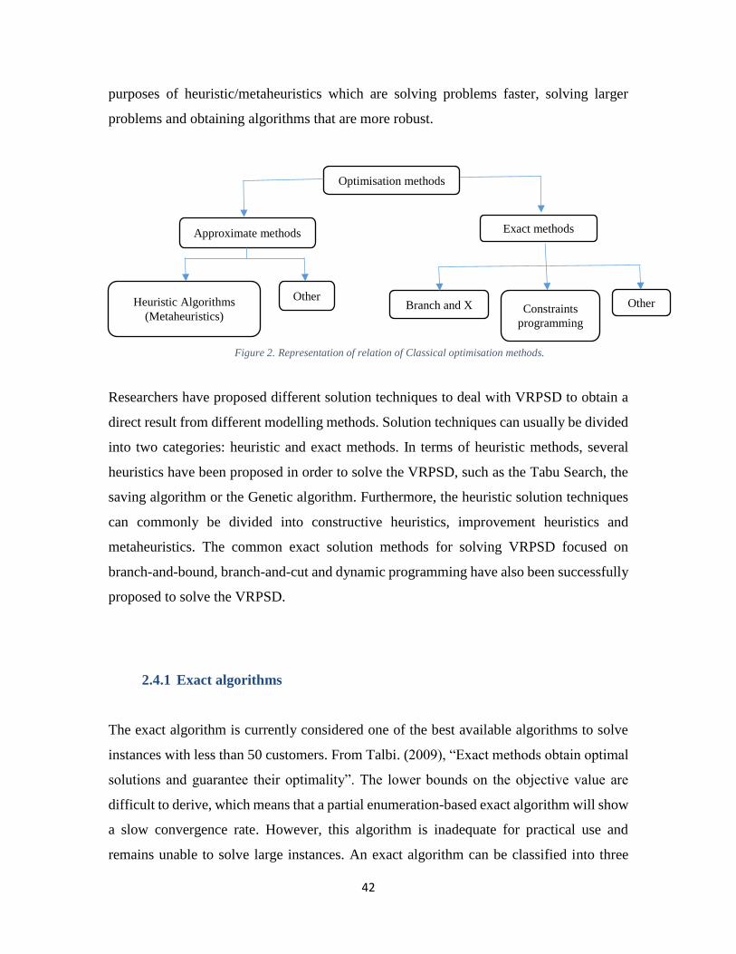
42

purposes of heuristic/metaheuristics which are solving problems faster, solving larger

problems and obtaining algorithms that are more robust.

Researchers have proposed different solution techniques to deal with VRPSD to obtain a

direct result from different modelling methods. Solution techniques can usually be divided

into two categories: heuristic and exact methods. In terms of heuristic methods, several

heuristics have been proposed in order to solve the VRPSD, such as the Tabu Search, the

saving algorithm or the Genetic algorithm. Furthermore, the heuristic solution techniques

can commonly be divided into constructive heuristics, improvement heuristics and

metaheuristics. The common exact solution methods for solving VRPSD focused on

branch-and-bound, branch-and-cut and dynamic programming have also been successfully

proposed to solve the VRPSD.

2.4.1 Exact algorithms

The exact algorithm is currently considered one of the best available algorithms to solve

instances with less than 50 customers. From Talbi. (2009), “Exact methods obtain optimal

solutions and guarantee their optimality”. The lower bounds on the objective value are

difficult to derive, which means that a partial enumeration-based exact algorithm will show

a slow convergence rate. However, this algorithm is inadequate for practical use and

remains unable to solve large instances. An exact algorithm can be classified into three

Optimisation methods

Approximate methods Exact methods

Heuristic Algorithms

(Metaheuristics)

Other Other

Constraints

programming

Branch and X

Figure 2. Representation of relation of Classical optimisation methods.

43

categories. The first category is dynamic programming which focuses on solving complex

problems by breaking problems down into simpler sub-problems. The second category is

the branch and X family of the algorithms (where the X represents the different variants,

such as Branch-and-Cut and Branch-and-Bound). These algorithms proposed in order to

solve Integer Linear Programming (ILP) and Mixed Integer Linear Programming problems

(MILP). In addition, these algorithms are considered to be one of the most popular methods

to solve problems such as VRPSD in an exact way. The third category is constraint

programming which is modelled by a set of variables connected by a constraints set. The

variables set can take their values from a finite domain of integers and the constraints set

could have a mathematical form. The VRPSD has received little attention in the literature

despite its applicability to many distribution systems. Different exact algorithms have been

developed to solve the VRPSD and these algorithms have been implemented with some

success in the problem. In addition, these algorithms look at the problem as a special case

of an integer or mixed integer programme that implements some form of branching to find

an optimal solution. Furthermore, the purpose of implementing these algorithms was to

provide a good solution for instances that are small and medium.

Both Stochastic Programs with Recourse (SPR) and Chance-Constrained Programs (CCP)

could be used to explicitly model the stochastic aspect of the VRPSD. Stewart et al. (1983)

described a Chance-Constrained Programs model in order to identify a set of vehicle routes

of minimum distance, subject to the constraint that the probability of failure of any route

is less than an allowable limit. Furthermore, they ignore recourse action costs and solve the

Chance-Constrained Programs model by transforming it into an equivalent deterministic

VRP, which then can be solved using standard solution techniques for the VRP. Laporte et

al. (1989) developed a branch and bound algorithm to solve exactly both a CCP model and

a bounded penalty model. Furthermore, there are two variants studies: (1) to minimise first

stage costs so that the probability of route failure does not exceed a present threshold; (2)

to minimise second stage costs so that the expected penalty of any route does not exceed a

fraction of its planned cost.

Stochastic Programs with Recourse models are considered as the most computationally

challenging for solving the VRPSD. Most of the Stochastic Programs with Recourse

44

models in the literature considered the VRPSD as a two-stage problem and all employ the

traditional recourse policy of (Dror et al., 1989). Although traditional recourse simplifies

the model to some extent, it overestimates the recourse cost particularly in the case of

multiple vehicles. Using the integer L-shaped method proposed by Laporte and Louveaux,

(1993, 1998); Gendreau et al. (1995) were the first to optimally solve a VRP with stochastic

customers and demands. Hjorring and Holt (1999) optimally solved the single VRPSD

using the integer L-shaped method following some probability distributions. To reduce

Central Processing Unit time, they introduced a tight lower bound and a general optimality

cut. To optimally solve a multiple VRPSD, Laporte et al. (2002) incorporated new

inequalities into the integer L-shaped method and are able to solve instances with up to 4

vehicles and 25 customers. The Poisson distributions were followed and normal

distributions were used when dealing with customer demands. The optimality of the results

is ensured by varying the number of the customers, and the number of vehicles used

(between two and four).

The branch-and-price procedure of (Christiansen and Lysgaard, 2007) has solved

optimality problem instances with many vehicles but fewer customers. A branch and price

algorithm has been proposed to solve the VRPSD; the problem is based on a partitioning

formation of the problem (Christiansen and Lysgaard., 2007). The number and sequence

of customers for each route designed are known when an integer solution of the problem

is not known. So the expected failure cost could be calculated before an integer solution is

known. Also, they adapted the instances to the VRPSD by assuming that customer demands

are Poisson random variables, with the mean demand for each customer, equal to the

deterministic value of demand given in the underlying VRP problem instance. Therefore,

the decision-maker is able to calculate the expected failure cost before an integer solution

is known.

Jabali et al. (2012) developed an exact algorithm for a variant of the vehicle routing

problem in which customer demands are stochastic. They made three main scientific

distributions. It first generalised the concept of partial routes defined by Hjorring and Holt,

(1999) for the single-vehicle case and by Laporte et al. (2002) for the multi-vehicle case.

It then proposed strengthened Lower Bounding Functionals based on these generalised

45

partial routes. Finally, it defined an exact separation algorithm for these Lower Bounding

Functionals. The computational results shown that some combinations of the proposed

Lower Bounding Functionals outperform the classical version. As a result, on a set of 270

benchmark instances, the number of optimally solved instances increased from 77 to 87,

which is significant in the context of stochastic vehicle routing. Furthermore, the results

confirmed the effectiveness of the proposed algorithm as measured by a substantial

reduction in the number of feasible solutions that have to be explicitly eliminated.

Gauvin et al., (2014) proposed a state-of-the-art branch-cut-and price algorithm for solving

VRPSD. Also, they formulated the VRPSD as a set partitioning model with additional

constraints and a subset of feasible routes are generated by using a dynamic programming

algorithm executed over a state-space graph. They also added the capacity cuts and subset-

row inequalities to the constraints in order to strengthen the linear relaxation of the

problem. Their algorithm combined 2 cycle elimination with 𝑛𝑔-routes, and as extensive

experiment results illustrate that their method is very competitive with the method

proposed by Christiansen and Lysgaard. (2007). Also, they showed the results of the

methodology by using Poisson distributed demands with integer expectation.

Computational results have shown that they can solve the majority of the instances

currently solved within the time limit of 20 minutes, when considering Poisson demands

with one decimal place.

An integer L-shaped method has been proposed (Jabali et al., 2014) to solve partial-route

inequalities for the multi-VRPSD. VRPSD was formulated as a two-stage stochastic

programming model and they extend and improve the integer L-shaped algorithm to solve

the problem. They introduced three Lower Bounding Functionals based on the generation

of general partial routes, alongside an exact separation procedure to identify violated cuts

to eliminate the number of infeasible solutions. Jabali et al. (2014) studied a problem where

a vehicle can arrive to a customer without enough capacity and cannot serve a customer.

Thus, the vehicle travels back to the central depot to reload and resume its planned route

at the position of failure. Their approach can solve a large number of instances by using

the normal distribution. Extensive numerical analysis was carried out to assess the

performance of the algorithm. The exact separation procedure was therefore able to solve

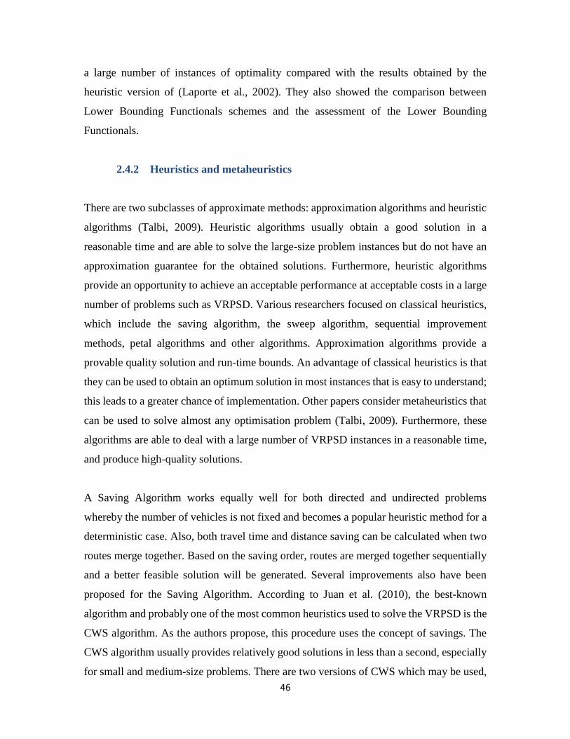
46

a large number of instances of optimality compared with the results obtained by the

heuristic version of (Laporte et al., 2002). They also showed the comparison between

Lower Bounding Functionals schemes and the assessment of the Lower Bounding

Functionals.

2.4.2 Heuristics and metaheuristics

There are two subclasses of approximate methods: approximation algorithms and heuristic

algorithms (Talbi, 2009). Heuristic algorithms usually obtain a good solution in a

reasonable time and are able to solve the large-size problem instances but do not have an

approximation guarantee for the obtained solutions. Furthermore, heuristic algorithms

provide an opportunity to achieve an acceptable performance at acceptable costs in a large

number of problems such as VRPSD. Various researchers focused on classical heuristics,

which include the saving algorithm, the sweep algorithm, sequential improvement

methods, petal algorithms and other algorithms. Approximation algorithms provide a

provable quality solution and run-time bounds. An advantage of classical heuristics is that

they can be used to obtain an optimum solution in most instances that is easy to understand;

this leads to a greater chance of implementation. Other papers consider metaheuristics that

can be used to solve almost any optimisation problem (Talbi, 2009). Furthermore, these

algorithms are able to deal with a large number of VRPSD instances in a reasonable time,

and produce high-quality solutions.

A Saving Algorithm works equally well for both directed and undirected problems

whereby the number of vehicles is not fixed and becomes a popular heuristic method for a

deterministic case. Also, both travel time and distance saving can be calculated when two

routes merge together. Based on the saving order, routes are merged together sequentially

and a better feasible solution will be generated. Several improvements also have been

proposed for the Saving Algorithm. According to Juan et al. (2010), the best-known

algorithm and probably one of the most common heuristics used to solve the VRPSD is the

CWS algorithm. As the authors propose, this procedure uses the concept of savings. The

CWS algorithm usually provides relatively good solutions in less than a second, especially

for small and medium-size problems. There are two versions of CWS which may be used,

47

parallel and sequential. CWS works in this way: savings are computed, followed by

ordering the savings list from the top to the bottom. Either the parallel version or sequential

version is then used to merge the feasible route starting from the top of the savings list.

Also, these savings are estimated between all customers and then decreasingly sorted.

Then, the bigger saving is always taken and used to merge the two associated routes. Juan

et al. (2010) proposed new algorithms based on CWS. The new algorithm is a multi-start

randomised approach called Simulation in Routing via the Generalised Clarke and Wright

Savings heuristic (SR-GCWS), in order to solve the VRPSD.

Mendoza et al. (2011) proposed three different constructive algorithms based on stochastic

programming with recourse formulation to solve multi-compartment VRPSD. One of these

algorithms is the CWS algorithm and the other two algorithms are different approaches of

a novel look-ahead heuristic that follows a route-first and cluster-second approach. They

tackled a generalisation of the VRPSD known as the multi-compartment VRPSD. In the

computational experiments, these three algorithms were tested on instances of up to 200

customers from the multi-compartment VRPSD with literature and compared with results

reported by Christiansen and Lysgaard (2007). These algorithms were able to obtain a good

solution in a short time. A multi-start search procedure was combined with the CWS

algorithm to solve VRPSD (Juan et al., 2013a). During designing the routes, part of the

vehicle capacity was considered safety stock and the remainder to be the capacity of the

vehicle used during the service. Their approach considered different levels of safety stocks.

For each of these levels, a different scenario is defined. After that, the approach solved

each scenario by integrating MCS inside a heuristic-randomisation process based on

randomised CWS. MCS was used to estimate the reliability of each route in the solution

obtained using the proposed method. This way, expected variable costs due to route failures

and can be naturally estimated even when customers’ demands follow a probability

distribution.

Most metaheuristics are adopted for an improvement phase. Also, metaheuristics

algorithms are able to generate an equally good solution even with a low-quality initial

solution. Metaheuristics are used in many applications and are both efficient and effective

at solving large and complex problems. In recent years, the application of metaheuristics

48

applied into a large number of areas, such as planning routing problems, robot planning,

scheduling, production, transportation and supply chain management. Metaheuristics are

especially implemented in solving VRPSD problems with a large size in a short time.

Metaheuristics are widely classified into three methods: population search, learning

mechanisms and local search. Greedy Randomised Adaptive Search Procedure (GRASP)

(Festa and Resende, 2009) and Variable Neighbourhood Search (VNS) (Hansen et al.,

2010) have been applied in VRPSD. The GRASP approach is one of the commonly

implemented metaheuristic algorithms in COPs. Each iteration of the GRASP approach

consists of two phases, construction and local search. Mendoza et al. (2015) proposed two

strategies to deal with route-duration constraints in the VRPSD which are GRASP

enhanced with Heuristic Concentration (HC). A set of randomised route-first and cluster-

second heuristics were used to build starting solutions followed by a variable

neighbourhood descent procedure for the local search phase. This approach followed the

Poisson distribution to test 40 instances of the classical VRPSD. GRASP-HC is thus able

to generate best solutions for all these instances compared with the literature.

Local search is a regularly used technique in COPs. It has been shown to be an effective

technique for producing better solutions to VRPSD instances and other variants. Several

local searches have been successfully implemented to solve VRPSD. The TS is one of the

local searches proposed by Haughland et al. (2007) in which demands are unknown at the

time when the districts are designed and appear only after the districting decisions are

determined. Multi-start heuristics have also been implemented and compared with the TS.

From the computational results, the TS therefore generated better solutions than the multi-

start heuristics. A TS heuristic is developed by Ak and Erera (2007) to find good solutions

to VRPSD instances with homogeneous customer demand distributions given the

alternative recourse strategy denoted by the paired locally coordinated operating scheme.

An Adaptive Large Neighbourhood Search (ALNS) heuristic was used by Lei et al. (2011)

to deal with the VRPSD. They generated initial solutions using the modification version of

the push forward insertion heuristic. At each iteration, a probabilistic mechanism is

implemented to choose the removal and insertion heuristic; one of the removal heuristics

is thus chosen randomly to destroy the current solution, and one of the insertion heuristics

49

is chosen randomly to repair the demand solution. The acceptance of the new solutions can

be obtained using the record to record travel algorithm. The objective is to minimise the

total deterministic costs of the first-stage solutions and the expected total cost of the

recourse action, as they model the problem as a stochastic programming model with

recourses. Modified Solomon benchmark instances are used in the experiments. The

computational results showed both the efficiency and the effectiveness of using the ALNS

algorithm. Experiments using the ALNS algorithm showed an improved performance of

the VRPSD.

Simulated annealing is another local search that can be proposed to find solutions to solve

the VRPSD instances. A simulated annealing was used by Goodson et al. (2012) to find an

optimal solution for the VRPSD. They utilised a simulated annealing framework in order

to demonstrate the potential of cyclic-order neighbourhoods to facilitate the discovery of

high quality a-priori solutions for the VRPSD. Without tailoring the solution procedure to

VRPSD, they are able to match 16 of 19 known optimal VRPSD solutions. Later, Goodson

(2015) subsequently modified the cyclic-order simulated annealing to solve the multi-

compartment VRPSD. The simulated annealing has two stages. In the first stage, solutions

are evaluated by scenarios, while the process of the second stage is to attempt to improve

the solution by exactly calculating the quality of the solution. In terms of the experiments,

they incorporated the estimation procedure into a cyclic-order-based simulated annealing

algorithm, in order to improve the best-known solution values for a number of instance

problems. They also discussed how the estimation procedure can be tested within local

search schemes.

Variable Neighbourhood Search (VNS) is quite a recent metaheuristic used for solving

optimisation problems based on a systematic change of the neighbourhood structures

within the search, in order to avoid local optima. It has been tested successfully in different

problems. It is based on a successive exploration of a set of predefined neighbourhoods to

achieve a better solution at each step. Biesinger et al. (2015) proposed VNS in order to

minimise the expected tour length through all clusters. They also proposed a multi-level

evaluation scheme to significantly reduce the time needed for solution evaluations. Two

different algorithms for finding an initial solution and three well-known neighbourhood

50

structures of permutations, are used within the VNS. In terms of the computational results,

a comparison to an exact approach showed that the VNS is able to achieve an optimal or

near-optimal solution in much shorter time. Large Neighbourhood Search (LNS) can be

interpreted as a special case of VNS where efficient procedures are designed to consider a

high number of neighbourhoods at the same time.

Oyola et al. (2016) extended the work of (Gendreau et al., 1996) to provide a

comprehensive review of the scientific literature on problems such as VRPSD and their

solution methods. The most important variants that have been studied are related to

stochastic demand. In addition, they surveyed numerous variants of the problem that have

been considered in the literature. The various solution methods that have been applied to

solve VRPSD, and other variants, are studied. In terms of the solution methods, the key

dichotomy is between exact solutions versus heuristic methods.

§2.5 Sim-Optimisation

The simulation-based optimisation (Sim-Opt) field is still a promising research line. A

number of studies have combined simulation and optimisation for different purposes, in

order to achieve an original resolution procedure, and also to help to deal with more

realistic/complex scenarios and to optimise large-scale problems (Glover et al., 1996,

1999). A number of Sim-Opt approaches have been proposed in the literature review by

using different criteria. A good comprehensive survey on the subject of simulation based

optimisation methods has been carried out by Andradottir (1998), and Fu et al. (2005). The

aim of the Sim-Opt approach is to obtain the optimal solution that can lead to minimise the

resources spent, while maximising the information found in a simulation experiment. A

review of the theory has been given by Long-Fei and Le-Yuan (2013) and they also

introduced some significant techniques for the Sim-Opt approach in detail. Note that

simulation contains several types e.g. MCS and optimisation contains several types e.g.

heuristic and metaheuristic. MCS has proved by Juan et al. (2011) to be extremely useful

for solving different problems with stochastic demands such as VRPSD. Therefore,

nowadays, the mixture of simulation with optimisation is becoming very popular and able

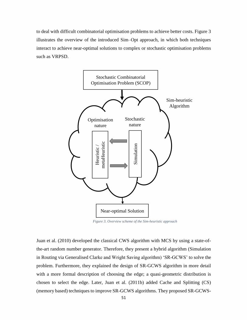
51

to deal with difficult combinatorial optimisation problems to achieve better costs. Figure 3

illustrates the overview of the introduced Sim–Opt approach, in which both techniques

interact to achieve near-optimal solutions to complex or stochastic optimisation problems

such as VRPSD.

Juan et al. (2010) developed the classical CWS algorithm with MCS by using a state-of-

the-art random number generator. Therefore, they present a hybrid algorithm (Simulation

in Routing via Generalised Clarke and Wright Saving algorithm) ‘SR-GCWS’ to solve the

problem. Furthermore, they explained the design of SR-GCWS algorithm in more detail

with a more formal description of choosing the edge; a quasi-geometric distribution is

chosen to select the edge. Later, Juan et al. (2011b) added Cache and Splitting (CS)

(memory based) techniques to improve SR-GCWS algorithms. They proposed SR-GCWS-

Figure 3. Overview scheme of the Sim-heuristic approach

Sim-heuristic

Algorithm

Heu

rist

ic /

met

aHeu

rist

ic

Optimisation

nature

Sim

ula

tion

Stochastic

nature

Stochastic Combinatorial

Optimisation Problem (SCOP)

Near-optimal Solution

52

CS probabilistic algorithm to efficiently achieve a set of alternative quasi-optimal solutions

for the problem in reasonable times. One idea is that they introduced some biased random

behaviour within the CWS algorithm, to perform a search process inside the space of

feasible solutions. Another idea is to divide the problem into small subsets and to solve

each one of these subsets by applying the same methodology.

The sim-heuristic can be used to find better results in different applications such as

transportation, manufacturing & production, healthcare, logistic & supply chain

management, and others. As an obvious example of using a sim-heuristic in the logistics

and transportation is VRPSD and (Juan et al., 2011a) considered different levels of the

safety stocks size in order to solve VRPSD and then solve the resulting scenarios. This is

performed by employing MCS, which allows for estimating the variable costs associated

with each candidate solution. Thus, between the multiple solutions generated for each

scenario, the solution with lowest expected total costs are stored as the best-found solution

associated with the corresponding safety-stock levels. Once the execution of the different

scenarios ends, the corresponding solutions are compared to each other and the one with

the lowest expected total costs is selected as the best-found routing plan.

In Juan et al. (2013) paper, they focused on VRPSD and discussed how Parallel and

Distributed Computing Systems can be employed to efficiently solve the VRPSD. MCS

can combine with biased randomised heuristics to handle complex real life problems with

uncertainty variables. Notice that the algorithm considered different levels of the safety

stocks size. For each of these levels, a different scenario is defined. Then, the algorithm

solves each scenario by integrating MCS inside a heuristic-randomisation process. This

way, expected variable costs due to route failures, can be naturally estimated even when

customer demands follow a non-normal probability distribution. Later, parallelisation

strategies are used to run multiple instances of the algorithm in a concurrent way.

Parallelisation strategies are used at two different levels: the first level, a parallel-execution

environment is designed in order to deal with the multiple-scenario analysis; the second

level is that several concurrent threads sharing a common memory or, alternatively, several

concurrent processes are considered during the algorithm execution for each scenario. In

terms of the computational results, they showed the steps to create biased randomisation

53

with benefits which are accuracy, speed, simplicity, and flexibility. This approach

represents several advantages such as an efficient, flexible and simple to solve number of

combinatorial optimisation problems, in different fields.

Another obvious example of a Sim-Opt approach is developed by Juan and Rabe (2013)

where the simulation is integrated with the heuristic/metaheuristic approach, that will

provide a dynamic feedback to the searching process, to improve the final result. Juan and

Rabe (2013) stated that sim-heuristics are an interesting approach for most real-life

problems and these methods can provide near-optimal solutions to complex real-life

problems within a reasonable computing time. Typically, given a Stochastic Combinatorial

Optimisation Problem (SCOP) instance, a heuristic/metaheuristic algorithm is run in order

to perform an oriented search inside the solution space. This iterative process aimed to find

feasible solutions with the best possible value, which is also expected to be near-optimal.

During the iterative search process, the algorithm must deal with the stochastic nature of

the SCOP instance. One natural way to do this is by taking advantage of the capabilities

offered by simulation methods to manage randomness. Obviously, one major drawback of

this approach is that the results are no longer expected to be optimal since sim-heuristics

combine two approximate methodologies. Nevertheless, real-life problems are sufficiently

complex and usually NP-hard even in their deterministic versions. Therefore, sim-

heuristics constitute a reasonably interesting alternative for most practical purposes since

they represent relatively simple and flexible methods that are able to provide near-optimal

solutions to complex real-life problems within reasonable computing times (Juan and Rabe,

2013) and (C´aceres-Cruz, 2013).

Several examples of a sim-heuristic application to different areas can be found in the Sim–

Opt literature. Thus, for instance, Gonzalez et al. (2012) combined MCS with routing

metaheuristics in order to solve the arc routing problem with stochastic demands. Juan et

al. (2014a) combined MCS with a scheduling metaheuristic to solve the permutation flow-

shop problem with stochastic processing times and (Juan et al., 2014b) combined MCS

with a routing metaheuristic in order to solve the inventory routing problem with stock-

outs and stochastic demands. Also, as illustrated in Cabrera et al. (2014), discrete-event

simulation can be used in combination with a metaheuristic to solve other COPs with

54

probabilistic constraints where the random behavior is conditioned by the time factor. After

completing an extensive review of related work by Juan et al. (2015), they described a

general methodology that allows for extending metaheuristics through simulation in order

to deal with stochastic combinatorial optimisation problems. Sim-heuristics allow models

for dealing with real-life uncertainty in a natural way by integrating simulation (in any of

its variants) into a metaheuristic-driven framework. These optimisation driven algorithms

rely on the fact that efficient metaheuristics already exist for the deterministic version of

the corresponding COP. Sim-heuristics also facilitate the introduction of risk and/or

reliability analysis criteria, during the assessment of alternative high-quality solutions to

SCOPs. They also provided several examples of applications in different fields in order to

illustrate the potential of the proposed methodology. So far, most sim-heuristic approaches

have focused on evaluation function and feasibility checking purposes and they have

employed either MCS or discrete-event simulation. We expect other types of simulation,

such as agent-based, to be increasingly implemented in sim-heuristic frameworks. Since

these simulation types require more computational effort and also analytical model

enhancement, methods appear to be a good alternative in many situations, particularly

when there is a linear analytical model for the problem.

2.5.1 Benefits of sim-heuristics approach

Cordeau et al. (2002) describe the main evaluation aspects of a metaheuristic, such as

accuracy, speed, simplicity, and flexibility. In general, the accuracy and speed aspects are

quite popular for measuring the performance of a solution method. The quality of solutions

used are represented by the numerical cost obtained in a given period of execution time.

However, each of the last two aspects has a different direction, which means that the

simplicity aspect is an important factor that is focused on easy implementation and

parameterisation. The flexibility is focused on the adaptation of a given method to be

modified for a different problem or constraint set. The natural adaptation to different

realistic scenarios is a feature demanded by the solution methods.

Bearing in mind these measured attributes, the main benefits of sim-heuristics over other

related approaches are listed below (C´aceres-Cruz, 2013):

55

The ever-increasing complexity of systems can be considered, such as the real-life

natural representation of variants in mathematical models (for example

stochasticity). Complex relations and real-life variables can be modelled in a

comprehensible way.

The use of different probabilistic properties (for example uncertainty levels) in

stochastic variables offers a more natural and efficient way to select the most proper

solution in different realistic scenarios. This offers a well-known starting point to

coordinate the execution of any sim-heuristic (parameterisation).

The generation of internal added-value information from simulation allows the

search to intensify in the solution space in the promising regions. In fact, it can

produce a set of solutions with different properties in order to offer different

solution-scenarios to the decision-maker.

Based on well-tested heuristics, the methods are relatively simple and easy to

implement, and can be adapted to account for new constraints (flexibility).

Furthermore, the general performance of heuristics is quite fast.

The natural and easy parallelisation of this general process can be combined with

multi-start-like approaches and different probabilistic properties.

§2.6 Chapter summary

The VRPSD is considered as one of the essential studies in the SVRP area. This problem

is widely studied due to the practical relevance of the applications. The research in this area

is growing faster than in the last decade. From the findings, current research on VRPSD

focused more on improving the collecting or delivering customer demand by minimisation

of costs which satisfy all the constraints. Some researchers are attempted to reduce the cost

by improving the routing of vehicles, other researchers defined the goal as minimising the

number of vehicles used. A central feature in VRPSD is the source of stochasticity in terms

of customer demand. Another important distinguishing feature of VRPSD is the recourse

policy, which described the actions to take in order to make the feasibility of the solution

route after a failure.

56

In terms of the robust model, a literature review showed that this could be a competitive

approach in addressing uncertainty for the VRP, when compared to the deterministic

solution, as it does not require distributing assumptions on the uncertainty. Also, a robust

model can be adapted to address the same uncertainty in the model as an alternative

approach to each other. However, this will require a different set of assumptions to follow,

which would result in different definitions of the uncertainty set. We have chosen few

studies that have addressed this issue with proposed different methods. Also, the robust

model can be applied in different areas such as robust inventory and revenue management.

An early development of the robust solution framework is able to obtain an optimal

solution that is immune to any realisation of uncertainty. Based on a literature review, it

can be concluded that the robust solution amounts to a clever management of the remaining

vehicle capacity compared to non-uniformly and uniformly distributing this slack over the

vehicles. We also verified that the robust solution is superior to simple strategies of

distributing the excess capacity among all vehicles. We noticed that such strategies

compete better with the robust solution as the network structure is more clustered.

However, an interesting future work is still needed to identify the best distribution of the

excess capacity in general.

There exists several versions of the problem, and a wide variety of exact and approximate

algorithms have been proposed for its solution. Exact algorithms can only solve relatively

small problems but a number of approximate algorithms have proved very satisfactory.

However, several promising avenues of research deserve more attention. A better heuristic

should be more flexible to accommodate the various side constraints encountered in most

of real-life applications. In terms of sim-heuristics, nowadays, the combination of Sim-Opt

is becoming quite popular in the research community. We presented several studies on sim-

heuristics methodology, which related to the combination of simulation with

heuristics/metaheuristic, in order to improve and to find a better way to solve combinatorial

optimisation problems, in particular, VRPSD. Additionally, the advantages of these

algorithms are that they are flexible, quite efficient and can be implemented in most

practical applications. Also, the uncertainty modelling feature of MCS mixed with efficient

and fast heuristics can create interesting approaches for real-life problems. Sim-heuristics

57

offer a practical perspective which is able to deal with more realistic scenarios: by

integrating MCS in the heuristic/metaheuristic, it is possible to naturally consider any

probabilistic distribution for modelling the random customer demand or job processing

times. To conclude a literature review showed that the use of sim-heuristics is a well-

established and increasingly relevant topic in combinatorial optimisation. Potential

applications of distributed computing to solve large-size VRPs with real-life constraints

have also been pointed out.

58

Chapter 3 : Robust routing model and Sim-

heuristic for VRPSD

§3.1 Introduction

One of the most challenging variants of the VRP is the VRPSD. The VRPSD is an NP-

hard problem in which a set of customers with random or stochastic demands, have to be

visited by a fleet of homogeneous vehicles that have a fixed capacity, and depart from a

central depot. The decision-maker has no knowledge of the demands that the vehicles will

encounter on a given route and each vehicle strives to meet all the customers’ demands

periodically. In terms of the demand, the demands of a given customer during each period

are modelled as being independent of those of other customers. Juan et al. (2015) provided

an extensive review of sim-heuristics and describe a general methodology that allows for

extending metaheuristics through simulation to solve SCOs. Sim-heuristics allow

modellers to deal with real-life uncertainty in a natural way by combining simulation into

a heuristic/metaheuristic. A robust solution approach has been studied using an exact

algorithm in (Sungur et al., 2007) to deal with VRPSD. Also, they used a high level of

sufficient management of the remaining vehicle capacity compared to uniformly and non-

uniformly distributing this slack for all the considered vehicles. This chapter is organised

as follows. In section 3.2, we present our contribution to this chapter. We proposed the

robust routing model in detail in section 3.3. The proposed approach for solving VRPSD

is presented in section 3.4. In section 3.5, we show all the computational experiments of

this chapter. We summarised the chapter in section 3.6.

§3.2 Contribution

Most of the existing approaches in the literature do not consider the robust routing model.

However, safety stock and reloading/restocking have been considered to minimise the total

cost. To the best of our knowledge, there is no research reported in the literature that

combines a robust routing model with a sim-heuristic to solve the VRPSD. One of the

major contributions of this study is the formulation of a robust routing model that

minimises deviation from the a-priori route, and the use of a sim-heuristic that combines

59

MCS and randomised CWS algorithms to provide a near-optimal solution for the VRPSD.

Our approach considers the robust routing model and sim-heuristic in order to solve

VRPSD. The methodology includes two stages. In the first stage, optimal a-priori routes

are generated using stochastic demand to satisfy all customer’s demand, which can be

achieved by devising a particular model and method. Because of the uncertainty of

customers’ demands, at some point along the route the vehicle capacity may be depleted

before all demands on the route have been satisfied. This situation is known as route failure.

In the second stage, the decision maker has to serve the failure by moving it to another

route, to minimise the sum of the expected total cost in all failed and successful routes. In

addition, when a vehicle capacity is exceeded, recourse actions have to be planned/

designed to make sure the feasibility of solutions in case of route failure.

In conclusion, most of the researchers have applied the sim-heuristic without using the

robustness. On the contrary, other researchers have considered the robustness using exact

algorithms to solve small instances. Therefore, in this chapter we proposed to build robust

solutions by developing a robust routing model and a sim-heuristic approach to minimise

the expected total cost. The robust routing model coupled with the sim-heuristic approach

proves to be a useful tool for solving VRPSD. The computational results have shown that

the robust routing model with a sim-heuristic improved the solutions, as well as showing

that the proposed robust routing model and sim-heuristic algorithm generated very good

solutions, compared to ones published in the literature.

§3.3 The robust routing model

VRPSD considers the problem of routing at minimum expected cost. Some of the standard

assumptions and definitions of the frequently used notations for the VRPSD are described

in the following. In general, the VRPSD can be defined as a complete graph 𝐺 = (𝑉, 𝐴, 𝐷).

Customers and depot are represented as: 𝑉 = {0, 1, 2, … , 𝑛} where 0 represents the central

depot and is treated as the source of demanded service and 1, 2, … , 𝑛 represent the number

of customers to be served. Also, it is assumed that the depot is fully interconnected with

the customers’ location 𝐴 = {(𝑖, 𝑗): 𝑖, 𝑗 ∈ 𝑉, 𝑖 ≠ 𝑗}. Every single vehicle has to start and end

its route at the depot with full capacity and each customer 𝑖 ∈ 𝑉 has a stochastic demand

60

𝐷 = {𝑑𝑖𝑗: 𝑖, 𝑗 ∈ 𝑉, 𝑖 ≠ 𝑗} and the demand appears when the vehicle arrives at the

customer’s location.

Each vehicle has a full capacity and when the total demand of the customer exceeds the

vehicle capacity, the planned route may not be achieved. The customer’s demand is the

most significant constraint in this problem. At the beginning, the demand is not known and

thus we are not able to design the routes with the optimal solution. However, we have to

follow two stages. In the first stage, we should design routes well in advance before the

real demands for each customer can be known. In the second stage, when the real demand

is known, we attempt to slightly adjust the pre-planned routes to satisfy the failed

customers. In addition, we assume that the customer’s demands are independently and

identically distributed. The customer’s demand, 𝑑𝑖, 𝑖 = 1,2, … , 𝑛 does not exceed the

vehicle’s capacity 𝑄 and it is a random variable which follows a discrete probability

distribution. Furthermore, the real customer’s demand is known when the vehicle arrives

at the customer’s location. It should be noted that 𝐾 represents the number of vehicles.

Designing the routes, route failure and recourse actions are the other important issues to

consider in this study. Defining the routes plays a key role in solving the VRPSD problem

and it enables us to generate a better solution through robust routes. The idea behind

designing robust routes is to obtain the best routes to meet uncertain customers’ demands.

Furthermore, it has the high possibility of achieving the required service quality at a lower

cost. Each vehicle has to start at the central depot and visits a number of customers and

then returns to the central depot. Clearly, the number of routes should be the same as the

number of the vehicles. A feasible solution to the VRPSD is a permutation of the customers

𝑠 = (𝑠(1), 𝑠(2), … , 𝑠(𝑛)) beginning and ending at the depot and 𝑠(1) = 𝑠(𝑛) = 0. A route

is considered as a failure when ∑ 𝑑𝑛𝑖(𝑟)𝑓𝑖=1 ≥ 𝑄, 𝑛𝑖(𝑟) represents the number of 𝑖 customer

that is served in a particular route 𝑟. It has to be an element in the customer set, i.e. 𝑛𝑖(𝑟) ∈

𝑉. In this case, the recourse actions are used such that a vehicle can continue to serve the

remaining customer’s demands where the customer demand is less than the remaining

vehicle capacity at the 𝑛𝑡ℎ customer. If ∑ 𝑑𝑛𝑖(𝑟)𝑓𝑖=1 = 𝑄, the recourse actions are not used

and the vehicle returns to the depot. If ∑ 𝑑𝑛𝑖(𝑟)𝑓𝑖=1 ≤ 𝑄, the recourse actions are used such

61

that the vehicle can serve other customers’ demands when they are less than the remaining

vehicle capacity. It should be noted that the recourse actions increase the total expected

transportation cost in terms of travel distance. However, some recourse or corrective

actions have to be applied to prevent the route failure and to ensure the solution feasibility.

Transportation cost is shown as 𝐶 which is used to define the VRPSD objective function;

Transportation cost 𝐶 = {𝑐𝑖𝑗, (𝑖, 𝑗): 𝑖, 𝑗 ∈ 𝑉, 𝑖 ≠ 𝑗} is usually expressed in different ways

such as the travelled distance between two customers or between a customer and the central

depot or vice versa. The cost is symmetric 𝑐𝑖𝑗 = 𝑐𝑗𝑖, and it satisfies the triangular

inequality 𝑐𝑖𝑗 ≤ 𝑐𝑖𝑢 + 𝑐𝑢𝑗, and it is clear that 𝑐𝑖𝑖 = 0. Furthermore, the additional cost is

calculated whenever a vehicle follows the a-priori route until the end, as there is enough

capacity to serve other customers’ demands where demand is less than the remaining

vehicle capacity. The cost matrix is a function of Euclidean distance and the Euclidean

distance can be calculated by using the following equation: where 𝑖𝑥 and 𝑖𝑦 are the 𝑥 and

𝑦 coordinates of the point 𝑖, respectively.

𝑐𝑖𝑗 = √(𝑖𝑥 − 𝑗𝑥)2 + (𝑖𝑦 − 𝑗𝑦)2 (1)

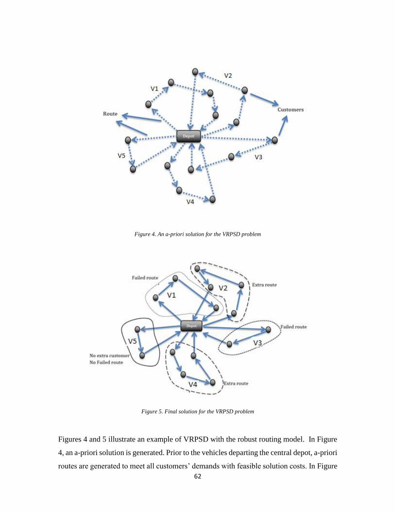
62

Figure 4. An a-priori solution for the VRPSD problem

Figure 5. Final solution for the VRPSD problem

Figures 4 and 5 illustrate an example of VRPSD with the robust routing model. In Figure

4, an a-priori solution is generated. Prior to the vehicles departing the central depot, a-priori

routes are generated to meet all customers’ demands with feasible solution costs. In Figure

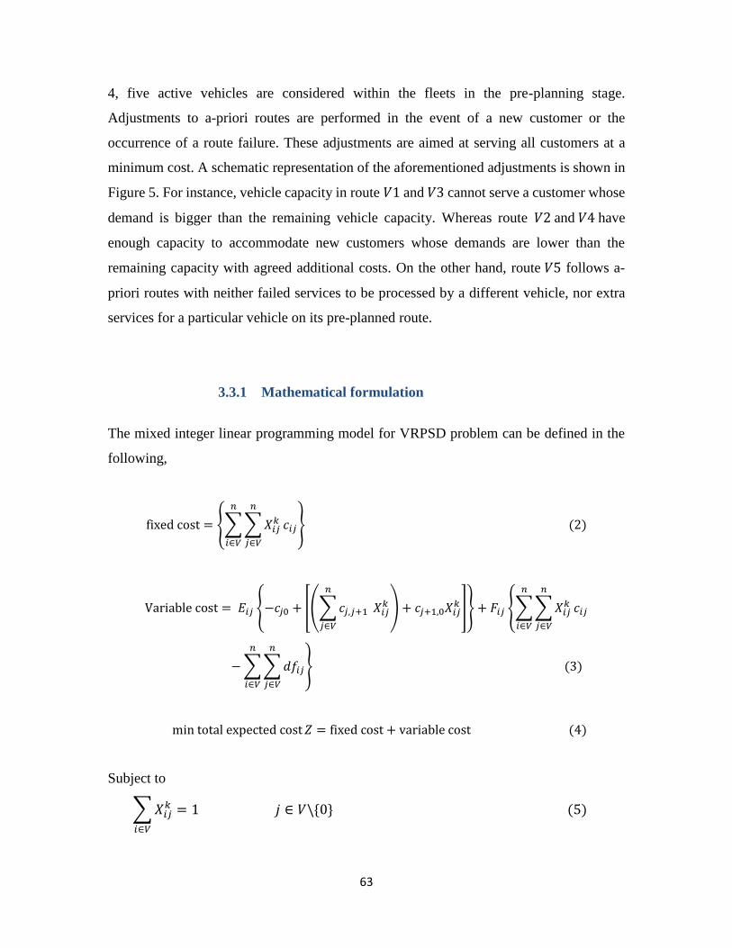
63

4, five active vehicles are considered within the fleets in the pre-planning stage.

Adjustments to a-priori routes are performed in the event of a new customer or the

occurrence of a route failure. These adjustments are aimed at serving all customers at a

minimum cost. A schematic representation of the aforementioned adjustments is shown in

Figure 5. For instance, vehicle capacity in route 𝑉1 and 𝑉3 cannot serve a customer whose

demand is bigger than the remaining vehicle capacity. Whereas route 𝑉2 and 𝑉4 have

enough capacity to accommodate new customers whose demands are lower than the

remaining capacity with agreed additional costs. On the other hand, route 𝑉5 follows a-

priori routes with neither failed services to be processed by a different vehicle, nor extra

services for a particular vehicle on its pre-planned route.

3.3.1 Mathematical formulation

The mixed integer linear programming model for VRPSD problem can be defined in the

following,

fixed cost = {∑∑𝑋𝑖𝑗𝑘

𝑛

𝑗∈𝑉

𝑐𝑖𝑗

𝑛

𝑖∈𝑉

} (2)

Variable cost = 𝐸𝑖𝑗 {−𝑐𝑗0 + [(∑𝑐𝑗,𝑗+1

𝑛

𝑗∈𝑉

𝑋𝑖𝑗𝑘) + 𝑐𝑗+1,0𝑋𝑖𝑗

𝑘 ]} + 𝐹𝑖𝑗 {∑∑𝑋𝑖𝑗𝑘

𝑛

𝑗∈𝑉

𝑐𝑖𝑗

𝑛

𝑖∈𝑉

− ∑∑𝑑𝑓𝑖𝑗

𝑛

𝑗∈𝑉

𝑛

𝑖∈𝑉

} (3)

min total expected cost 𝑍 = fixed cost + variable cost (4)

Subject to

∑𝑋𝑖𝑗𝑘

𝑖∈𝑉

= 1 𝑗 ∈ 𝑉\{0} (5)

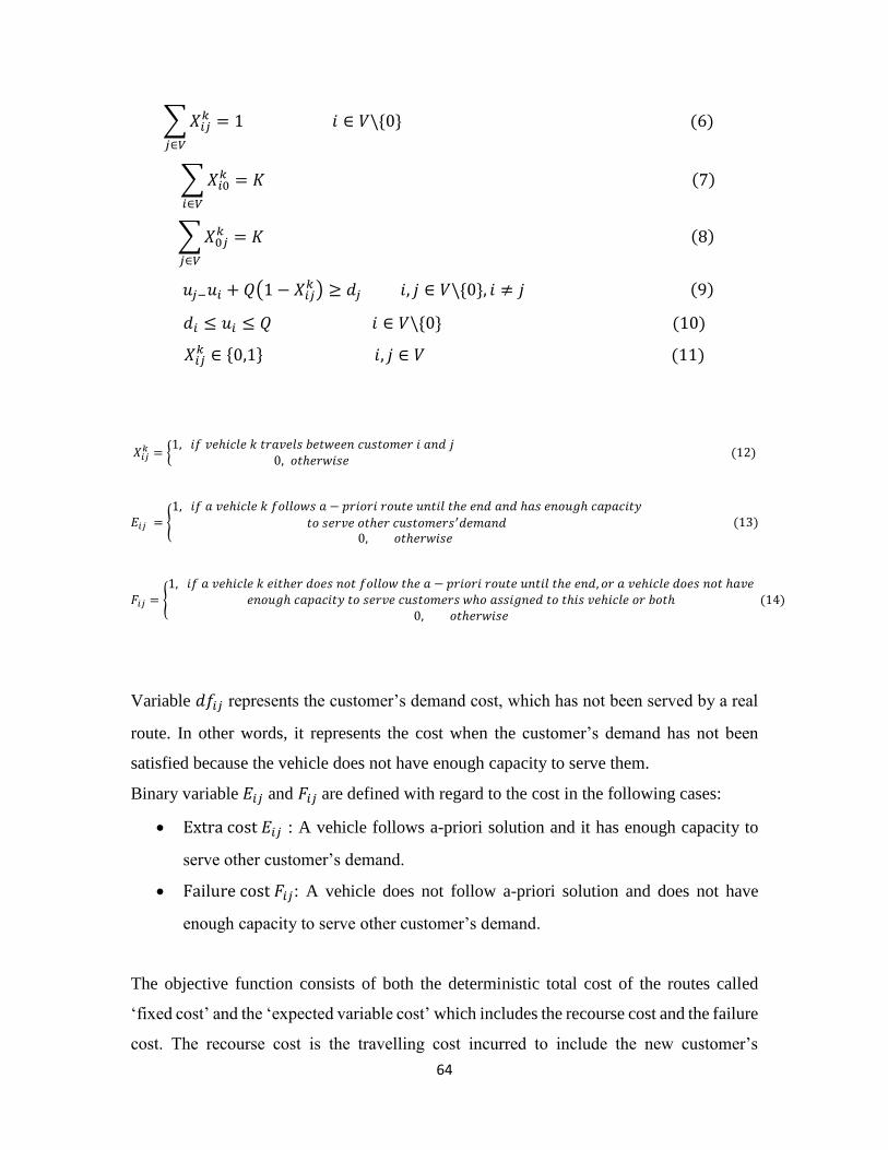
64

∑𝑋𝑖𝑗𝑘

𝑗∈𝑉

= 1 𝑖 ∈ 𝑉\{0} (6)

∑𝑋𝑖0𝑘

𝑖∈𝑉

= 𝐾 (7)

∑𝑋0𝑗𝑘

𝑗∈𝑉

= 𝐾 (8)

𝑢𝑗−𝑢𝑖 + 𝑄(1 − 𝑋𝑖𝑗𝑘) ≥ 𝑑𝑗 𝑖, 𝑗 ∈ 𝑉\{0}, 𝑖 ≠ 𝑗 (9)

𝑑𝑖 ≤ 𝑢𝑖 ≤ 𝑄 𝑖 ∈ 𝑉\{0} (10)

𝑋𝑖𝑗𝑘 ∈ {0,1} 𝑖, 𝑗 ∈ 𝑉 (11)

𝑋𝑖𝑗𝑘 = {

1, 𝑖𝑓 𝑣𝑒ℎ𝑖𝑐𝑙𝑒 𝑘 𝑡𝑟𝑎𝑣𝑒𝑙𝑠 𝑏𝑒𝑡𝑤𝑒𝑒𝑛 𝑐𝑢𝑠𝑡𝑜𝑚𝑒𝑟 𝑖 𝑎𝑛𝑑 𝑗0, 𝑜𝑡ℎ𝑒𝑟𝑤𝑖𝑠𝑒

(12)

𝐸𝑖𝑗 = {1, 𝑖𝑓 𝑎 𝑣𝑒ℎ𝑖𝑐𝑙𝑒 𝑘 𝑓𝑜𝑙𝑙𝑜𝑤𝑠 𝑎 − 𝑝𝑟𝑖𝑜𝑟𝑖 𝑟𝑜𝑢𝑡𝑒 𝑢𝑛𝑡𝑖𝑙 𝑡ℎ𝑒 𝑒𝑛𝑑 𝑎𝑛𝑑 ℎ𝑎𝑠 𝑒𝑛𝑜𝑢𝑔ℎ 𝑐𝑎𝑝𝑎𝑐𝑖𝑡𝑦

𝑡𝑜 𝑠𝑒𝑟𝑣𝑒 𝑜𝑡ℎ𝑒𝑟 𝑐𝑢𝑠𝑡𝑜𝑚𝑒𝑟𝑠′𝑑𝑒𝑚𝑎𝑛𝑑 0, 𝑜𝑡ℎ𝑒𝑟𝑤𝑖𝑠𝑒

(13)

𝐹𝑖𝑗 = {1, 𝑖𝑓 𝑎 𝑣𝑒ℎ𝑖𝑐𝑙𝑒 𝑘 𝑒𝑖𝑡ℎ𝑒𝑟 𝑑𝑜𝑒𝑠 𝑛𝑜𝑡 𝑓𝑜𝑙𝑙𝑜𝑤 𝑡ℎ𝑒 𝑎 − 𝑝𝑟𝑖𝑜𝑟𝑖 𝑟𝑜𝑢𝑡𝑒 𝑢𝑛𝑡𝑖𝑙 𝑡ℎ𝑒 𝑒𝑛𝑑, 𝑜𝑟 𝑎 𝑣𝑒ℎ𝑖𝑐𝑙𝑒 𝑑𝑜𝑒𝑠 𝑛𝑜𝑡 ℎ𝑎𝑣𝑒

𝑒𝑛𝑜𝑢𝑔ℎ 𝑐𝑎𝑝𝑎𝑐𝑖𝑡𝑦 𝑡𝑜 𝑠𝑒𝑟𝑣𝑒 𝑐𝑢𝑠𝑡𝑜𝑚𝑒𝑟𝑠 𝑤ℎ𝑜 𝑎𝑠𝑠𝑖𝑔𝑛𝑒𝑑 𝑡𝑜 𝑡ℎ𝑖𝑠 𝑣𝑒ℎ𝑖𝑐𝑙𝑒 𝑜𝑟 𝑏𝑜𝑡ℎ 0, 𝑜𝑡ℎ𝑒𝑟𝑤𝑖𝑠𝑒

(14)

Variable 𝑑𝑓𝑖𝑗 represents the customer’s demand cost, which has not been served by a real

route. In other words, it represents the cost when the customer’s demand has not been

satisfied because the vehicle does not have enough capacity to serve them.

Binary variable 𝐸𝑖𝑗 and 𝐹𝑖𝑗 are defined with regard to the cost in the following cases:

Extra cost 𝐸𝑖𝑗 : A vehicle follows a-priori solution and it has enough capacity to

serve other customer’s demand.

Failure cost 𝐹𝑖𝑗: A vehicle does not follow a-priori solution and does not have

enough capacity to serve other customer’s demand.

The objective function consists of both the deterministic total cost of the routes called

‘fixed cost’ and the ‘expected variable cost’ which includes the recourse cost and the failure

cost. The recourse cost is the travelling cost incurred to include the new customer’s

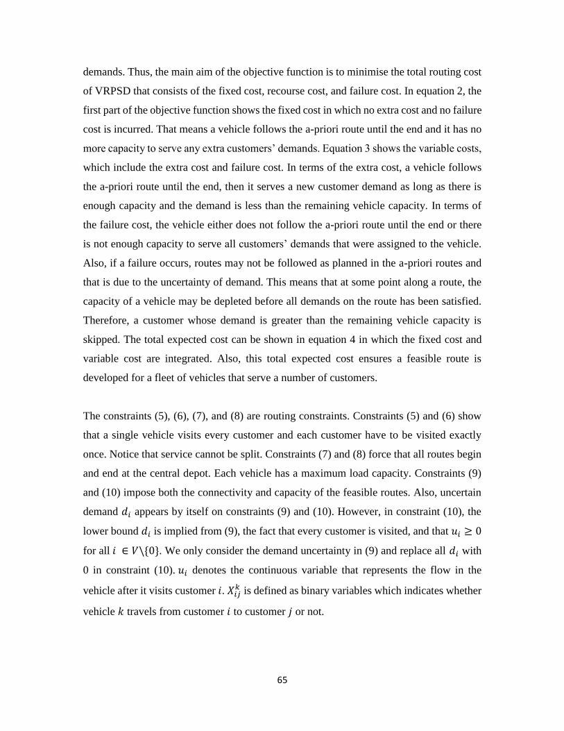
65

demands. Thus, the main aim of the objective function is to minimise the total routing cost

of VRPSD that consists of the fixed cost, recourse cost, and failure cost. In equation 2, the

first part of the objective function shows the fixed cost in which no extra cost and no failure

cost is incurred. That means a vehicle follows the a-priori route until the end and it has no

more capacity to serve any extra customers’ demands. Equation 3 shows the variable costs,

which include the extra cost and failure cost. In terms of the extra cost, a vehicle follows

the a-priori route until the end, then it serves a new customer demand as long as there is

enough capacity and the demand is less than the remaining vehicle capacity. In terms of

the failure cost, the vehicle either does not follow the a-priori route until the end or there

is not enough capacity to serve all customers’ demands that were assigned to the vehicle.

Also, if a failure occurs, routes may not be followed as planned in the a-priori routes and

that is due to the uncertainty of demand. This means that at some point along a route, the

capacity of a vehicle may be depleted before all demands on the route has been satisfied.

Therefore, a customer whose demand is greater than the remaining vehicle capacity is

skipped. The total expected cost can be shown in equation 4 in which the fixed cost and

variable cost are integrated. Also, this total expected cost ensures a feasible route is

developed for a fleet of vehicles that serve a number of customers.

The constraints (5), (6), (7), and (8) are routing constraints. Constraints (5) and (6) show

that a single vehicle visits every customer and each customer have to be visited exactly

once. Notice that service cannot be split. Constraints (7) and (8) force that all routes begin

and end at the central depot. Each vehicle has a maximum load capacity. Constraints (9)

and (10) impose both the connectivity and capacity of the feasible routes. Also, uncertain

demand 𝑑𝑖 appears by itself on constraints (9) and (10). However, in constraint (10), the

lower bound 𝑑𝑖 is implied from (9), the fact that every customer is visited, and that 𝑢𝑖 ≥ 0

for all 𝑖 ∈ 𝑉\{0}. We only consider the demand uncertainty in (9) and replace all 𝑑𝑖 with

0 in constraint (10). 𝑢𝑖 denotes the continuous variable that represents the flow in the

vehicle after it visits customer 𝑖. 𝑋𝑖𝑗𝑘 is defined as binary variables which indicates whether

vehicle 𝑘 travels from customer 𝑖 to customer 𝑗 or not.

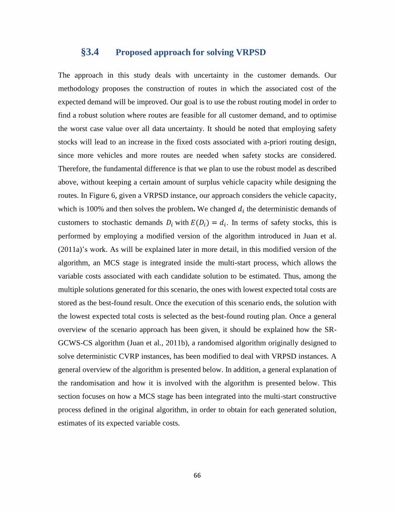
66

§3.4 Proposed approach for solving VRPSD

The approach in this study deals with uncertainty in the customer demands. Our

methodology proposes the construction of routes in which the associated cost of the

expected demand will be improved. Our goal is to use the robust routing model in order to

find a robust solution where routes are feasible for all customer demand, and to optimise

the worst case value over all data uncertainty. It should be noted that employing safety

stocks will lead to an increase in the fixed costs associated with a-priori routing design,

since more vehicles and more routes are needed when safety stocks are considered.

Therefore, the fundamental difference is that we plan to use the robust model as described

above, without keeping a certain amount of surplus vehicle capacity while designing the

routes. In Figure 6, given a VRPSD instance, our approach considers the vehicle capacity,

which is 100% and then solves the problem. We changed 𝑑𝑖 the deterministic demands of

customers to stochastic demands 𝐷𝑖 with 𝐸(𝐷𝑖) = 𝑑𝑖. In terms of safety stocks, this is

performed by employing a modified version of the algorithm introduced in Juan et al.

(2011a)’s work. As will be explained later in more detail, in this modified version of the

algorithm, an MCS stage is integrated inside the multi-start process, which allows the

variable costs associated with each candidate solution to be estimated. Thus, among the

multiple solutions generated for this scenario, the ones with lowest expected total costs are

stored as the best-found result. Once the execution of this scenario ends, the solution with

the lowest expected total costs is selected as the best-found routing plan. Once a general

overview of the scenario approach has been given, it should be explained how the SR-

GCWS-CS algorithm (Juan et al., 2011b), a randomised algorithm originally designed to

solve deterministic CVRP instances, has been modified to deal with VRPSD instances. A

general overview of the algorithm is presented below. In addition, a general explanation of

the randomisation and how it is involved with the algorithm is presented below. This

section focuses on how a MCS stage has been integrated into the multi-start constructive

process defined in the original algorithm, in order to obtain for each generated solution,

estimates of its expected variable costs.

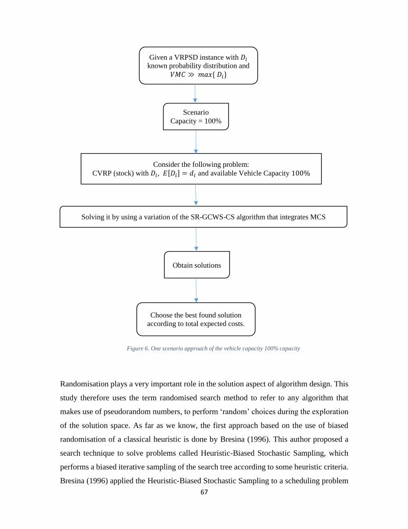
67

Randomisation plays a very important role in the solution aspect of algorithm design. This

study therefore uses the term randomised search method to refer to any algorithm that

makes use of pseudorandom numbers, to perform ‘random’ choices during the exploration

of the solution space. As far as we know, the first approach based on the use of biased

randomisation of a classical heuristic is done by Bresina (1996). This author proposed a

search technique to solve problems called Heuristic-Biased Stochastic Sampling, which

performs a biased iterative sampling of the search tree according to some heuristic criteria.

Bresina (1996) applied the Heuristic-Biased Stochastic Sampling to a scheduling problem

Figure 6. One scenario approach of the vehicle capacity 100% capacity

Given a VRPSD instance with 𝐷𝑖

known probability distribution and

𝑉𝑀𝐶 ≫ 𝑚𝑎𝑥{ 𝐷𝑖}

Scenario

Capacity = 100%

Consider the following problem:

CVRP (stock) with 𝐷𝑖, 𝐸 𝐷𝑖 = 𝑑𝑖 and available Vehicle Capacity 100%

Choose the best found solution

according to total expected costs.

Solving it by using a variation of the SR-GCWS-CS algorithm that integrates MCS

Obtain solutions

68

and concluded that this approach outperforms a greedy search within a small number of

samples. Other non-symmetric (biased) distributions can also be used to induce

randomness into an algorithm. GRASP is considered to be one of the most popular

randomised search methods. As described in Festa and Resende (2009), GRASP

algorithms have been applied to solve a wide set of problems like scheduling, routing,

logic, partitioning and location. Resende and Ribeiro (2010) described several tasks, such

as the basic components of GRASP and alternative randomised greedy construction

schemes. GRASP is a multi-start metaheuristic or iterative process for combinatorial

optimisation problems which use uniform random numbers and a restricted candidate list

to explore the solution space. There are two phases at each iteration: construction and local

search. The construction phase generates a new solution by randomising a classical

heuristic, whilst the local search phase improves the previously constructed solution. At

the end of this multi-start process, the local search aims to keep the best overall solution as

the result. Juan et al. (2011c) discussed the use of probabilistic or randomised algorithms

to deal with VRP with non-smooth objective functions. The idea of the general framework

in the study by Juan et al. (2011c) is the MIRHA local search. This combined classical

greedy heuristic with pseudorandom varieties from a different non-symmetric probability

distribution, is developed in order to add a biased random into classical heuristics. The

MIRHA approach was explained more clearly with a pseudo-code published in (Juan et al.,

2013b).

69

Figure 7. Uniform randomisation vs. biased randomisation (Juan et al. 2014)

To avoid losing the ‘common sense’ behind the heuristic, GRASP proposes to consider a

restricted list of candidates. This is a sub-list including just some of the most promising

movements, namely the ones at the top of the list, before applying a uniform randomisation

in the order in which the elements of that restricted list are selected (see left-hand side of

Figure 7). In this way, a deterministic procedure is transformed into a randomised

algorithm that can be encapsulated into a multi-start process, while most of the logic or

common sense behind the original heuristic is still respected. The MIRHA approach goes

one step further, and instead of restricting the list of candidates, it assigns different

probabilities of being selected to each potential movement in the sorted list. In this way,

the elements at the top of the list receive a higher probability of being selected than those

at the bottom of the list, although all elements could potentially be selected. It should be

noted that by doing so, this not only avoids the issue of selecting the proper size of the

restricted list, but also guarantees that the probabilities of being selected are always

proportional to the position of each element in the list (see the right-hand side of Figure 7).

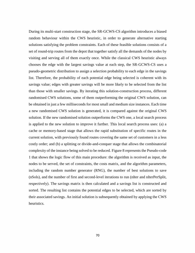
70

During its multi-start construction stage, the SR-GCWS-CS algorithm introduces a biased

random behaviour within the CWS heuristic, in order to generate alternative starting

solutions satisfying the problem constraints. Each of these feasible solutions consists of a

set of round-trip routes from the depot that together satisfy all the demands of the nodes by

visiting and serving all of them exactly once. While the classical CWS heuristic always

chooses the edge with the largest savings value at each step, the SR-GCWS-CS uses a

pseudo-geometric distribution to assign a selection probability to each edge in the savings

list. Therefore, the probability of each potential edge being selected is coherent with its

savings value; edges with greater savings will be more likely to be selected from the list

than those with smaller savings. By iterating this solution-construction process, different

randomised CWS solutions, some of them outperforming the original CWS solution, can

be obtained in just a few milliseconds for most small and medium size instances. Each time

a new randomised CWS solution is generated, it is compared against the original CWS

solution. If the new randomised solution outperforms the CWS one, a local search process

is applied to the new solution to improve it further. This local search process uses: (a) a

cache or memory-based stage that allows the rapid substitution of specific routes in the

current solution, with previously found routes covering the same set of customers in a less

costly order; and (b) a splitting or divide-and-conquer stage that allows the combinatorial

complexity of the instance being solved to be reduced. Figure 8 represents the Pseudo-code

1 that shows the logic flow of this main procedure: the algorithm is received as input, the

nodes to be served, the set of constraints, the costs matrix, and the algorithm parameters,

including the random number generator (RNG), the number of best solutions to save

(nSols), and the number of first and second-level iterations to run (nIter and nIterPerSplit,

respectively). The savings matrix is then calculated and a savings list is constructed and

sorted. The resulting list contains the potential edges to be selected, which are sorted by

their associated savings. An initial solution is subsequently obtained by applying the CWS

heuristics.

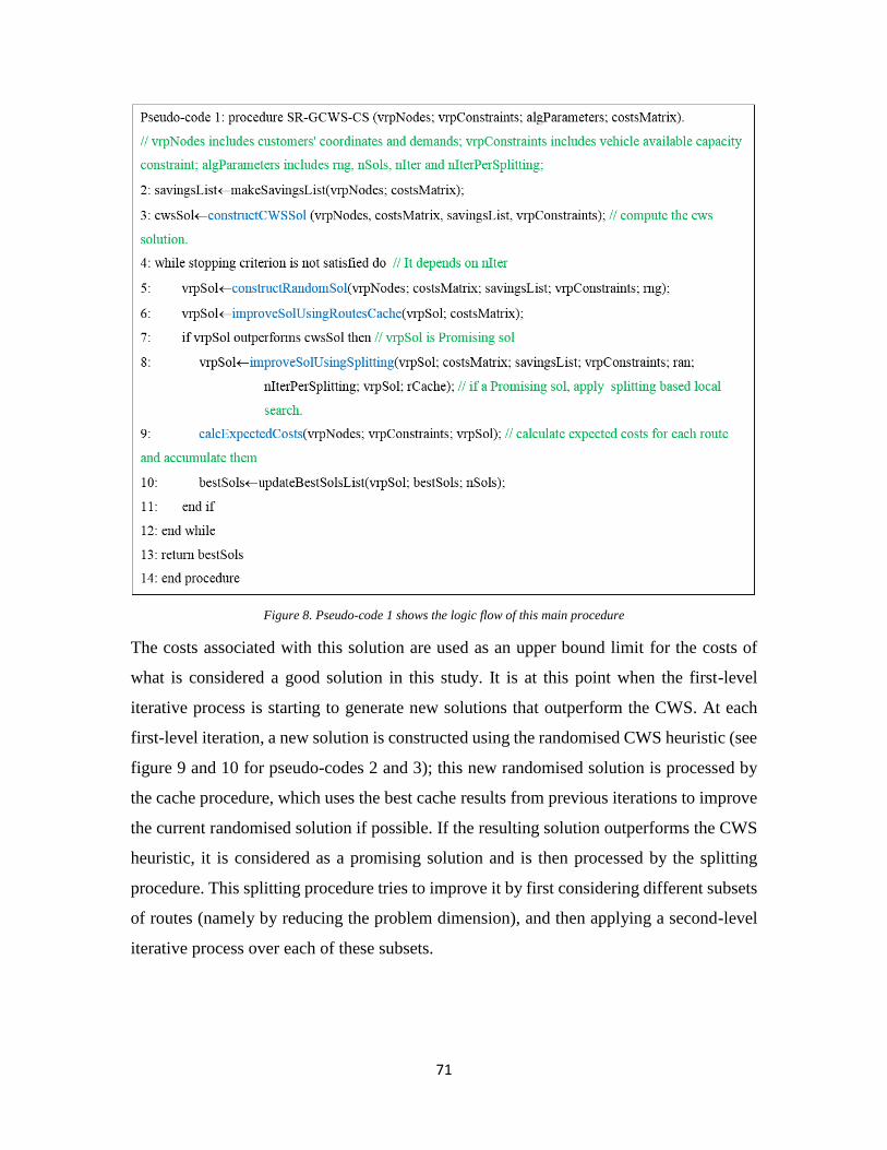
71

Figure 8. Pseudo-code 1 shows the logic flow of this main procedure

The costs associated with this solution are used as an upper bound limit for the costs of

what is considered a good solution in this study. It is at this point when the first-level

iterative process is starting to generate new solutions that outperform the CWS. At each

first-level iteration, a new solution is constructed using the randomised CWS heuristic (see

figure 9 and 10 for pseudo-codes 2 and 3); this new randomised solution is processed by

the cache procedure, which uses the best cache results from previous iterations to improve

the current randomised solution if possible. If the resulting solution outperforms the CWS

heuristic, it is considered as a promising solution and is then processed by the splitting

procedure. This splitting procedure tries to improve it by first considering different subsets

of routes (namely by reducing the problem dimension), and then applying a second-level

iterative process over each of these subsets.

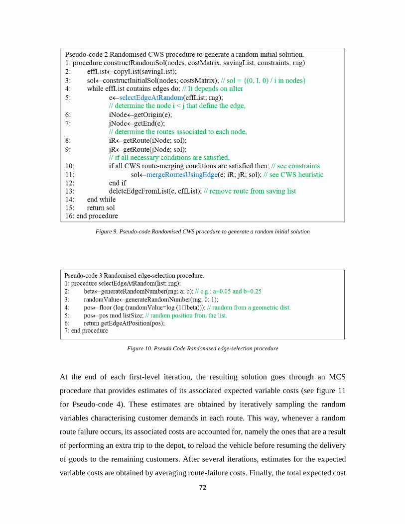
72

Figure 9. Pseudo-code Randomised CWS procedure to generate a random initial solution

Figure 10. Pseudo Code Randomised edge-selection procedure

At the end of each first-level iteration, the resulting solution goes through an MCS

procedure that provides estimates of its associated expected variable costs (see figure 11

for Pseudo-code 4). These estimates are obtained by iteratively sampling the random

variables characterising customer demands in each route. This way, whenever a random

route failure occurs, its associated costs are accounted for, namely the ones that are a result

of performing an extra trip to the depot, to reload the vehicle before resuming the delivery

of goods to the remaining customers. After several iterations, estimates for the expected

variable costs are obtained by averaging route-failure costs. Finally, the total expected cost

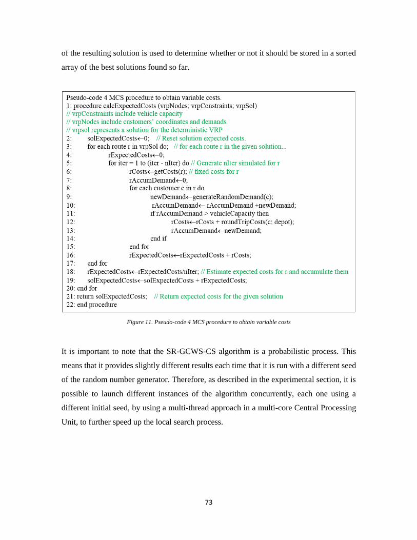
73

of the resulting solution is used to determine whether or not it should be stored in a sorted

array of the best solutions found so far.

Figure 11. Pseudo-code 4 MCS procedure to obtain variable costs

It is important to note that the SR-GCWS-CS algorithm is a probabilistic process. This

means that it provides slightly different results each time that it is run with a different seed

of the random number generator. Therefore, as described in the experimental section, it is

possible to launch different instances of the algorithm concurrently, each one using a

different initial seed, by using a multi-thread approach in a multi-core Central Processing

Unit, to further speed up the local search process.

74

§3.5 Computational experiments

The computational experiments have been conducted using well known benchmark

problems from the literature. Juan et al. ( 2013) modified the benchmarks and they decided

to employ a natural generalisation of several classical CVRP instances by using random

customer demands, instead of constant ones, in order to deal with VRPSD. We used the

same benchmarks in order to compare our results with the literature. This approach has at

least three advantages: (1) all data details, including customers coordinates and random

demands, are given, so that other researchers can use the same data sets for verifying and

benchmarking purposes; (2) we are using a well-known set of instances which includes a

diversity of clustered and disperse problems of different sizes; and (3) our VRPSD results

for each instance can be compared with the best known solution in the literature. This

approach has at least three advantages: (1) all data details, including customers coordinates

and random demands, are given, so that other researchers can use the same data sets for

verifying and benchmarking purposes; (2) we are using a well-known set of instances

which includes a diversity of clustered and disperse problems of different sizes; and (3) our

VRPSD results for each instance can be compared with the best known solution in the

literature.

The algorithm described in this paper are implemented using Java application. In the

experiments, a Macintosh HD on 2.3 GHz Intel HD Graphics 4000 1024 MB with Intel

Core i7 with 4 GB 1600 MHz DDR3 has been used to perform the computational

experiments. Java is used since it is being an object-oriented language and it facilitates the

quick development of a prototype. Notice that no fine-tuning process was carried out, since

one of our aims was to show that our approach is robust and can provide efficient solutions

to VRPSD problem with very few adjustments. We have tested our algorithms on several

instances originally developed for the Capacitated VRP. The instances consisted of a set of

55 classical CVRP instances on the so-called A, B, E, F, M, and P benchmarks, which

details (in terms of customers’ coordinates, deterministic demands and vehicle capacity)

and are available at https://www.coin-

or.org/SYMPHONY/branchandcut/VRP/data/index.htm.old. This link contains data sets

for the CVRP.

75

For example A-n80-k10 is an instance of class A with 80 customers which has to be solved

with a 10 routes solution. The number of customers is in the range from 20 to 121. We used

the same customers and vehicle maximum capacity as in the original benchmark data. So,

for each instance, we keep all customer coordinates and vehicle capacities the same, but

we change 𝑑𝑖, the deterministic demands of a customer 𝑖 to stochastic demands 𝐷𝑖

with 𝐸 𝐷𝑖 = 𝑑𝑖. In other words, we considered the demand of each customer as a random

variable following a well-known statistical distribution with a given mean and a variance.

To determine the standard parameter setting of the approach, we performed extensive tests

solving VRPSD benchmark instances, considering the objective function in which the

expected total costs are primarily minimised. Parameter of the algorithm is Geometric

distribution. We selected a Geometric distribution for modelling demands, although any

other distribution with a known mean could have been used instead. In fact, real-world

problem historical data would be used to model each customer’s demand by a different

probability distribution, which can be naturally supported by our simulation-based

approach. Also, a Geometric probability distribution, which only has one parameter, has

proven to be an excellent option (Juan et al., 2010).

We considered a 100% of the vehicle maximum capacity. Both the average and best

solution for each approach are composed of three main parts including - fixed costs,

expected variable costs and expected total costs that are obtained. Notice that this strategy

always provides pseudo-optimal solutions in terms of fixed costs. However, since no safety

stock is used, there is a chance that these solutions can suffer from route failures. By using

the robust model, some route failures can be avoided. Hopefully, this might lead to new

solutions with slightly higher fixed costs but with lower expected variable costs. At the

end, these alternative solutions can present lower expected total costs, which are the ones

to be minimised. We reported the cost of the average solution of the approaches of 10 runs

of each instance. We have chosen 10 runs because we compared our results with those seen

by (Juan et al. 2013) who chose the average of 10 runs. The best solution of each instance

is based on the best run of these 10 runs. Furthermore, the best solution of both the average

and best for each instance is shown in bold in both expected total costs; the improvements

between these approaches is also included. The row entitled as ‘average’ computes the

76

average of the 55 rows above, for these approaches. The bottom row in tables shows the

average value of the results for each approach, for all instances of the problems.

The computational results are shown in the tables 1, 2, 3 and 4. These tables clearly showed

the results for “A”, “B”, “E”, “F”, “M” and “P” instances by using sim-heuristic with and

without the robust routing model and the approach by (Juan et al., 2013). These tables

reported the results obtained for all 55 classical instances. The results for a particular

instance are shown in the following columns. In all tables in the study, the first column

represents the instance number and the second column represents instance name, which

includes the class, the number of the customers and the number of routes. Tables 1, 2, 3

and 4 illustrated the results of three distinct approaches implemented in this chapter.

Namely: (Juan et al., 2013) approach and two novel approaches that firstly, do not account

for robustness in the solution and subsequently takes robustness into consideration. In each

of these approaches, the average and the best solution is computed in each instance. The

columns “Juan et al., 2013” summarises the average and the best results obtained by

applying (Juan et al., 2013) approach. The columns ‘sim-heuristic without robustness’ and

sim-heuristic with robustness summarise the average and best results obtained by these

approaches.

The solution quality is given in terms of the relative deviation from the current solution.

Moreover, the percentage (%) improvement between the approaches is calculated as

follows; the Current Solutions (CS), the Old Solutions

(OS); 𝑃𝑒𝑟𝑐𝑒𝑛𝑡𝑎𝑔𝑒 (%) 𝑖𝑚𝑝𝑟𝑜𝑣𝑒𝑚𝑒𝑛𝑡 = (𝑂𝑆−𝐶𝑆

𝐶𝑆) ∗ 100 . Where CS represents the

Current Solution denoting the expected total cost of the solution found by our approach

with the model, whereas OS represents the Old Solution indicating the expected total cost

of the solution in the literature. The % improvements are expressed as a percentage value

between two approaches and the respective % improvements between expected total costs

are shown in the tables. The following abbreviations are used:

E. V. Cost: Expected Variable Cost for the approach represented in all tables as E.

V. Cost.

F. Cost: Fixed Cost for the approach represented in all tables as F. Cost.

77

E. T. Cost: Expected Total Cost for the approach in all tables as E. T. Cost

Tables 1 and 2 illustrate the results of the two novel approaches that firstly, do not account

for robustness in the solution and subsequently take robustness into consideration. In these

tables, we summarised the results obtained by sim-heuristic without and with the

robustness where the vehicle capacity considered as 100%. The comparative results

between sim-heuristic with and without robustness are as follows: in terms of the average

results, the most fixed cost results obtained by the sim-heuristic with robustness are always

greater than or equal to those obtained by sim-heuristic without robustness. However, there

are 22 instances where the results of the fixed costs obtained by the sim-heuristic with

robustness are lower than those obtained by sim-heuristic without robustness. The expected

variable cost results obtained by sim-heuristic with robustness are always lower than those

obtained by sim-heuristic without robustness. Notice that there is only one instance which

is E-n76-k14 that has the same expected variable costs. In terms of the total expected costs,

the results obtained by sim-heuristic with robustness are lower than those obtained without

robustness. The deviation in solution between the approaches have been computed and

displayed in the last two columns in Tables 1 and 2. In terms of the average % improvement

between these approaches: in 10 out of 55 instances the % improvement of the expected

total cost is less than 1%, in 34 out of 55 it is between 1 % to 3 % and in 11 out of 55

instances it is more than 3%.

In terms of the best result, the most fixed cost results obtained by the sim-heuristic with

robustness are always greater than or equal to those obtained by sim-heuristic without

robustness. However, there are 14 instances where the fixed costs results obtained by the

sim-heuristic with robustness are lower than those obtained by sim-heuristic without

robustness. The expected variable cost results obtained by sim-heuristic with robustness

are always lower than those obtained by sim-heuristic without robustness. Notice that there

is only one instance, E-n76-k14, which has the same expected variable costs. Also, the total

expected cost results obtained by sim-heuristic with robustness are lower than those

obtained by sim-heuristic without robustness. Consequently, the results obtained by sim-

heuristic with robustness are better than sim-heuristic without robustness. In terms of the

best % improvement between these approaches: in 10 out of 55 instances the %

78

improvement of the expected total cost is less than 1%, in 35 out of 55 it is between 1% to

3% and in 10 out of 55 instances it is more than 3%.

Notice that, in most instances this % improvement is not small and sometimes it can reach

4% in both the average and best column, which means that using the sim-heuristic without

robustness can lead to an increase in the expected total cost, because a vehicle can travel

back without any restrictions. As it can be observed that sim-heuristic with robust routing

model clearly outperformed the sim-heuristic without robustness (average % improvement

about 1.99%, best % improvement about 2.10%; 54 out of 55 instances are considered

because the E-n76-k14 has no % improvement in both average and best result and therefore

this instance is not taken into the total average presented in the bottom row).

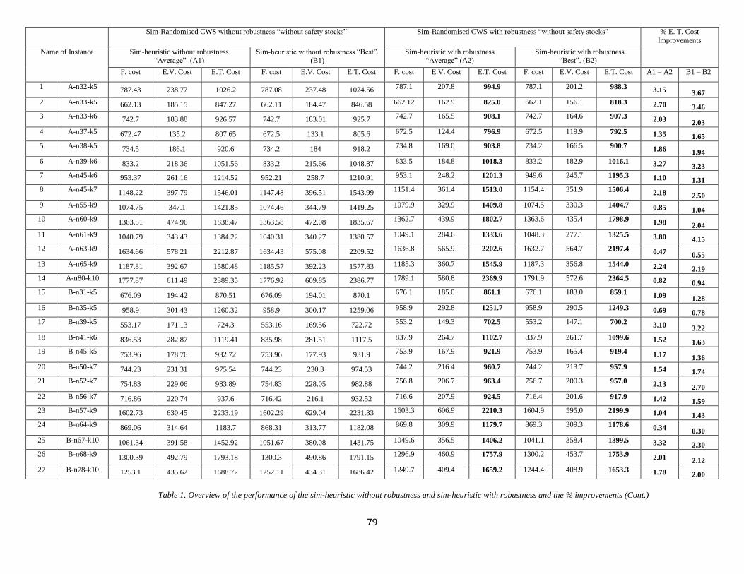
79

Sim-Randomised CWS without robustness “without safety stocks” Sim-Randomised CWS with robustness “without safety stocks” % E. T. Cost

Improvements

Name of Instance Sim-heuristic without robustness

“Average” (A1)

Sim-heuristic without robustness “Best”.

(B1)

Sim-heuristic with robustness

“Average” (A2)

Sim-heuristic with robustness

“Best”. (B2)

F. cost E.V. Cost E.T. Cost F. cost E.V. Cost E.T. Cost F. cost E.V. Cost E.T. Cost F. cost E.V. Cost E.T. Cost A1 – A2 B1 – B2

1 A-n32-k5 787.43 238.77 1026.2 787.08 237.48 1024.56 787.1 207.8 994.9 787.1 201.2 988.3 3.15 3.67

2 A-n33-k5 662.13 185.15 847.27 662.11 184.47 846.58 662.12 162.9 825.0 662.1 156.1 818.3 2.70 3.46

3 A-n33-k6 742.7 183.88 926.57 742.7 183.01 925.7 742.7 165.5 908.1 742.7 164.6 907.3 2.03 2.03

4 A-n37-k5 672.47 135.2 807.65 672.5 133.1 805.6 672.5 124.4 796.9 672.5 119.9 792.5 1.35 1.65

5 A-n38-k5 734.5 186.1 920.6 734.2 184 918.2 734.8 169.0 903.8 734.2 166.5 900.7 1.86 1.94

6 A-n39-k6 833.2 218.36 1051.56 833.2 215.66 1048.87 833.5 184.8 1018.3 833.2 182.9 1016.1 3.27 3.23

7 A-n45-k6 953.37 261.16 1214.52 952.21 258.7 1210.91 953.1 248.2 1201.3 949.6 245.7 1195.3 1.10 1.31

8 A-n45-k7 1148.22 397.79 1546.01 1147.48 396.51 1543.99 1151.4 361.4 1513.0 1154.4 351.9 1506.4 2.18 2.50

9 A-n55-k9 1074.75 347.1 1421.85 1074.46 344.79 1419.25 1079.9 329.9 1409.8 1074.5 330.3 1404.7 0.85 1.04

10 A-n60-k9 1363.51 474.96 1838.47 1363.58 472.08 1835.67 1362.7 439.9 1802.7 1363.6 435.4 1798.9 1.98 2.04

11 A-n61-k9 1040.79 343.43 1384.22 1040.31 340.27 1380.57 1049.1 284.6 1333.6 1048.3 277.1 1325.5 3.80 4.15

12 A-n63-k9 1634.66 578.21 2212.87 1634.43 575.08 2209.52 1636.8 565.9 2202.6 1632.7 564.7 2197.4 0.47 0.55

13 A-n65-k9 1187.81 392.67 1580.48 1185.57 392.23 1577.83 1185.3 360.7 1545.9 1187.3 356.8 1544.0 2.24 2.19

14 A-n80-k10 1777.87 611.49 2389.35 1776.92 609.85 2386.77 1789.1 580.8 2369.9 1791.9 572.6 2364.5 0.82 0.94

15 B-n31-k5 676.09 194.42 870.51 676.09 194.01 870.1 676.1 185.0 861.1 676.1 183.0 859.1 1.09 1.28

16 B-n35-k5 958.9 301.43 1260.32 958.9 300.17 1259.06 958.9 292.8 1251.7 958.9 290.5 1249.3 0.69 0.78

17 B-n39-k5 553.17 171.13 724.3 553.16 169.56 722.72 553.2 149.3 702.5 553.2 147.1 700.2 3.10 3.22

18 B-n41-k6 836.53 282.87 1119.41 835.98 281.51 1117.5 837.9 264.7 1102.7 837.9 261.7 1099.6 1.52 1.63

19 B-n45-k5 753.96 178.76 932.72 753.96 177.93 931.9 753.9 167.9 921.9 753.9 165.4 919.4 1.17 1.36

20 B-n50-k7 744.23 231.31 975.54 744.23 230.3 974.53 744.2 216.4 960.7 744.2 213.7 957.9 1.54 1.74

21 B-n52-k7 754.83 229.06 983.89 754.83 228.05 982.88 756.8 206.7 963.4 756.7 200.3 957.0 2.13 2.70

22 B-n56-k7 716.86 220.74 937.6 716.42 216.1 932.52 716.6 207.9 924.5 716.4 201.6 917.9 1.42 1.59

23 B-n57-k9 1602.73 630.45 2233.19 1602.29 629.04 2231.33 1603.3 606.9 2210.3 1604.9 595.0 2199.9 1.04 1.43

24 B-n64-k9 869.06 314.64 1183.7 868.31 313.77 1182.08 869.8 309.9 1179.7 869.3 309.3 1178.6 0.34 0.30

25 B-n67-k10 1061.34 391.58 1452.92 1051.67 380.08 1431.75 1049.6 356.5 1406.2 1041.1 358.4 1399.5 3.32 2.30

26 B-n68-k9 1300.39 492.79 1793.18 1300.3 490.86 1791.15 1296.9 460.9 1757.9 1300.2 453.7 1753.9 2.01 2.12

27 B-n78-k10 1253.1 435.62 1688.72 1252.11 434.31 1686.42 1249.7 409.4 1659.2 1244.4 408.9 1653.3 1.78 2.00

Table 1. Overview of the performance of the sim-heuristic without robustness and sim-heuristic with robustness and the % improvements (Cont.)

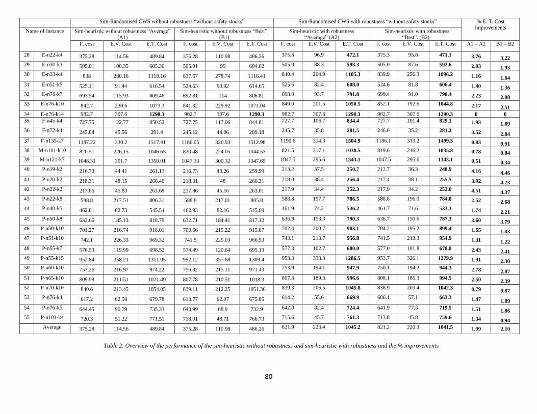
80

Sim-Randomised CWS without robustness “without safety stocks” Sim-Randomised CWS with robustness “without safety stocks” % E. T. Cost Improvements

Name of Instance Sim-heuristic without robustness “Average” (A1)

Sim-heuristic without robustness “Best”. (B1)

Sim-heuristic with robustness “Average” (A2)

Sim-heuristic with robustness “Best”. (B2)

F. cost E.V. Cost E.T. Cost F. cost E.V. Cost E.T. Cost F. cost E.V. Cost E.T. Cost F. cost E.V. Cost E.T. Cost A1 – A2 B1 – B2

28 E-n22-k4 375.28 114.56 489.84 375.28 110.98 486.26 375.3 96.9 472.1 375.3 95.8 471.1 3.76 3.22

29 E-n30-k3 505.01 100.35 605.36 505.01 99 604.02 505.0 88.3 593.3 505.0 87.6 592.6 2.03 1.93

30 E-n33-k4 838 280.16 1118.16 837.67 278.74 1116.41 840.4 264.9 1105.3 839.9 256.3 1096.2 1.16 1.84

31 E-n51-k5 525.11 91.44 616.54 524.63 90.02 614.65 525.6 82.4 608.0 524.6 81.8 606.4 1.40 1.36

32 E-n76-k7 693.54 115.93 809.46 692.81 114 806.81 698.0 93.7 791.8 699.4 91.0 790.4 2.23 2.08

33 E-n76-k10 842.7 230.6 1073.3 841.32 229.92 1071.04 849.0 201.5 1050.5 852.1 192.6 1044.8 2.17 2.51

34 E-n76-k14 982.7 307.6 1290.3 982.7 307.6 1290.3 982.7 307.6 1290.3 982.7 307.6 1290.3 0 0

35 F-n45-k4 727.75 122.77 850.52 727.75 117.06 844.81 727.7 106.7 834.4 727.7 101.4 829.1 1.93 1.89

36 F-n72-k4 245.84 45.56 291.4 245.12 44.06 289.18 245.7 35.8 281.5 246.0 35.2 281.2 3.52 2.84

37 F-n135-k7 1187.22 330.2 1517.41 1186.05 326.93 1512.98 1190.6 314.3 1504.9 1186.1 313.2 1499.3 0.83 0.91

38 M-n101-k10 820.51 226.15 1046.65 820.48 224.05 1044.53 821.5 217.1 1038.5 819.6 216.2 1035.8 0.78 0.84

39 M-n121-k7 1048.31 301.7 1350.01 1047.33 300.32 1347.65 1047.5 295.6 1343.1 1047.5 295.6 1343.1 0.51 0.34

40 P-n19-k2 216.73 44.41 261.13 216.73 43.26 259.99 213.2 37.5 250.7 212.7 36.3 248.9 4.16 4.46

41 P-n20-k2 218.31 48.15 266.46 218.31 48 266.31 218.0 38.4 256.4 217.4 38.1 255.5 3.92 4.23

42 P-n22-k2 217.85 45.83 263.69 217.86 45.16 263.01 217.9 34.4 252.3 217.9 34.2 252.0 4.51 4.37

43 P-n22-k8 588.8 217.51 806.31 588.8 217.01 805.8 588.8 197.7 786.5 588.8 196.0 784.8 2.52 2.68

44 P-n40-k5 462.81 82.73 545.54 462.93 82.16 545.09 461.9 74.2 536.2 461.7 71.6 533.3 1.74 2.21

45 P-n50-k8 633.66 185.13 818.79 632.71 184.41 817.12 636.9 153.3 790.3 636.7 150.6 787.3 3.60 3.79

46 P-n50-k10 701.27 216.74 918.01 700.66 215.22 915.87 702.4 200.7 903.1 704.2 195.2 899.4 1.65 1.83

47 P-n51-k10 742.1 226.33 969.32 741.5 225.03 966.53 743.1 213.7 956.8 741.5 213.3 954.9 1.31 1.22

48 P-n55-k7 576.53 119.99 696.52 574.49 120.64 695.13 577.3 102.7 680.0 577.0 101.8 678.8 2.43 2.41

49 P-n55-k15 952.84 358.21 1311.05 952.12 357.68 1309.4 953.3 333.3 1286.5 953.7 326.1 1279.9 1.91 2.30

50 P-n60-k10 757.26 216.97 974.22 756.32 215.11 971.43 753.9 194.1 947.9 750.1 194.2 944.3 2.78 2.87

51 P-n65-k10 809.98 211.51 1021.49 807.78 210.51 1018.3 807.3 189.3 996.6 808.1 186.3 994.5 2.50 2.39

52 P-n70-k10 840.6 213.45 1054.05 839.11 212.25 1051.36 839.3 206.5 1045.8 838.9 203.4 1042.3 0.79 0.87

53 P-n76-k4 617.2 62.58 679.78 613.77 62.07 675.85 614.2 55.6 669.9 606.1 57.1 663.3 1.47 1.89

54 P-n76-k5 644.45 90.79 735.33 643.99 88.9 732.9 642.0 82.4 724.4 641.9 77.5 719.5 1.51 1.86

55 P-n101-k4 720.3 51.22 771.51 718.01 48.71 766.73 715.6 45.7 761.3 713.8 45.8 759.6 1.34 0.94

Average 375.28 114.56 489.84 375.28 110.98 486.26 821.9 223.4 1045.2 821.2 220.3 1041.5 1.99 2.10

Table 2. Overview of the performance of the sim-heuristic without robustness and sim-heuristic with robustness and the % improvements

81

Tables 3 and 4 compared the results of two distinct approaches, namely (Juan et al., 2013)

approach and sim-heuristic with robustness; the deviation in solution between two

approaches has been computed. The columns that are related to solutions obtained with the

algorithm presented in (Juan et al., 2013) approach, when they used a percentage of the

vehicle maximum capacity during the design stage, are shown in the tables 3 and 4. Also,

they apply the simulation after the local search process. The solutions obtained by sim-

heuristic with robustness where the vehicle capacity is considered during the design stage

as 100%, are also presented in tables 3 and 4. We summarised the results obtained by sim-

heuristic with robustness and (Juan et al., 2013) approach in these tables. The comparative

results between the approach proposed by (Juan et al., 2013) and sim-heuristic with

robustness are as follows; in terms of the average result, the fixed cost results obtained by

sim-heuristic with robustness are always higher or equal to those obtained by (Juan et al.,

2013) approach. However, there are 11 instances where the fixed costs results obtained by

sim-heuristic with robustness are lower than those obtained by (Juan et al., 2013) approach.

The expected variable cost results obtained by sim-heuristic with robustness are always

lower than those obtained by (Juan et al., 2013) approach. Also, the expected total cost

results obtained by sim-heuristic with robustness are lower than those obtained by (Juan et

al., 2013) approach. Moreover, in terms of the best result, the fixed cost results obtained

by sim-heuristic with robustness are always higher or equal to those obtained by (Juan et

al., 2013) approach. However, there are 10 instances where the fixed costs results obtained

by sim-heuristic with robustness are lower than those obtained by (Juan et al., 2013)

approach. The expected variable cost results obtained by sim-heuristic with robustness are

always lower than those obtained by (Juan et al., 2013) approach. The expected total cost

results obtained by sim-heuristic with robustness are lower than those in (Juan et al., 2013)

approach.

For each instance, it is interesting to observe the evolution of the improvements between

(Juan et al., 2013) approach and sim-heuristic with robustness. Therefore, in Tables 3 and

4, the respective improvements between (Juan et al., 2013) approach and sim-heuristic with

robustness are presented in the last two columns. The results showed that the sim-heuristic

with robustness is able to obtain high quality solutions when compared with (Juan et al.,

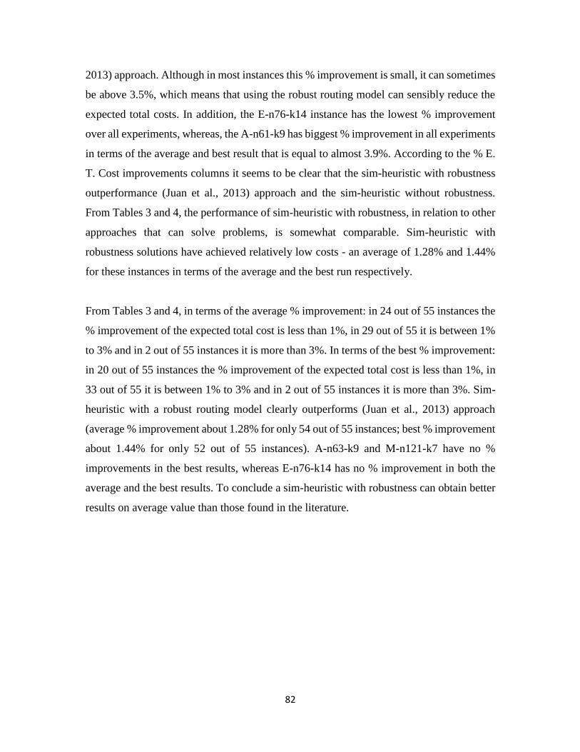
82

2013) approach. Although in most instances this % improvement is small, it can sometimes

be above 3.5%, which means that using the robust routing model can sensibly reduce the

expected total costs. In addition, the E-n76-k14 instance has the lowest % improvement

over all experiments, whereas, the A-n61-k9 has biggest % improvement in all experiments

in terms of the average and best result that is equal to almost 3.9%. According to the % E.

T. Cost improvements columns it seems to be clear that the sim-heuristic with robustness

outperformance (Juan et al., 2013) approach and the sim-heuristic without robustness.

From Tables 3 and 4, the performance of sim-heuristic with robustness, in relation to other

approaches that can solve problems, is somewhat comparable. Sim-heuristic with

robustness solutions have achieved relatively low costs - an average of 1.28% and 1.44%

for these instances in terms of the average and the best run respectively.

From Tables 3 and 4, in terms of the average % improvement: in 24 out of 55 instances the

% improvement of the expected total cost is less than 1%, in 29 out of 55 it is between 1%

to 3% and in 2 out of 55 instances it is more than 3%. In terms of the best % improvement:

in 20 out of 55 instances the % improvement of the expected total cost is less than 1%, in

33 out of 55 it is between 1% to 3% and in 2 out of 55 instances it is more than 3%. Sim-

heuristic with a robust routing model clearly outperforms (Juan et al., 2013) approach

(average % improvement about 1.28% for only 54 out of 55 instances; best % improvement

about 1.44% for only 52 out of 55 instances). A-n63-k9 and M-n121-k7 have no %

improvements in the best results, whereas E-n76-k14 has no % improvement in both the

average and the best results. To conclude a sim-heuristic with robustness can obtain better

results on average value than those found in the literature.

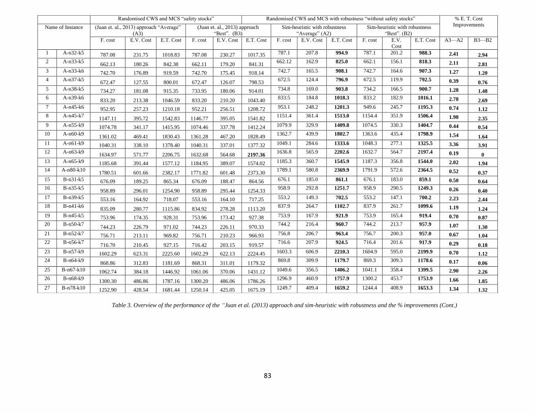
83

Randomised CWS and MCS “safety stocks” Randomised CWS and MCS with robustness “without safety stocks” % E. T. Cost Improvements Name of Instance (Juan et. al., 2013) approach “Average”

(A3)

(Juan et. al., 2013) approach

“Best”. (B3)

Sim-heuristic with robustness

“Average” (A2)

Sim-heuristic with robustness

“Best”. (B2)

F. cost E.V. Cost E.T. Cost F. cost E.V. Cost E.T. Cost F. cost E.V. Cost E.T. Cost F. cost E.V.

Cost

E.T. Cost A3—A2 B3—B2

1 A-n32-k5 787.08 231.75 1018.83 787.08 230.27 1017.35 787.1 207.8 994.9 787.1 201.2 988.3 2.41 2.94

2 A-n33-k5 662.13 180.26 842.38 662.11 179.20 841.31

662.12 162.9 825.0 662.1 156.1 818.3 2.11 2.81

3 A-n33-k6 742.70 176.89 919.59 742.70 175.45 918.14 742.7 165.5 908.1 742.7 164.6 907.3 1.27 1.20

4 A-n37-k5 672.47 127.55 800.01 672.47 126.07 798.53

672.5 124.4 796.9 672.5 119.9 792.5 0.39 0.76

5 A-n38-k5 734.27 181.08 915.35 733.95 180.06 914.01 734.8 169.0 903.8 734.2 166.5 900.7 1.28 1.48

6 A-n39-k6 833.20 213.38 1046.59 833.20 210.20 1043.40

833.5 184.8 1018.3 833.2 182.9 1016.1 2.78 2.69

7 A-n45-k6 952.95 257.23 1210.18 952.21 256.51 1208.72 953.1 248.2 1201.3 949.6 245.7 1195.3 0.74 1.12

8 A-n45-k7 1147.11 395.72 1542.83 1146.77 395.05 1541.82

1151.4 361.4 1513.0 1154.4 351.9 1506.4 1.98 2.35

9 A-n55-k9 1074.78 341.17 1415.95 1074.46 337.78 1412.24 1079.9 329.9 1409.8 1074.5 330.3 1404.7 0.44 0.54

10 A-n60-k9 1361.02 469.41 1830.43 1361.28 467.20 1828.49

1362.7 439.9 1802.7 1363.6 435.4 1798.9 1.54 1.64

11 A-n61-k9 1040.31 338.10 1378.40 1040.31 337.01 1377.32 1049.1 284.6 1333.6 1048.3 277.1 1325.5 3.36 3.91

12 A-n63-k9 1634.97 571.77 2206.75 1632.68 564.68 2197.36

1636.8 565.9 2202.6 1632.7 564.7 2197.4 0.19 0

13 A-n65-k9 1185.68 391.44 1577.12 1184.95 389.07 1574.02 1185.3 360.7 1545.9 1187.3 356.8 1544.0 2.02 1.94

14 A-n80-k10 1780.51 601.66 2382.17 1771.82 601.48 2373.30

1789.1 580.8 2369.9 1791.9 572.6 2364.5 0.52 0.37

15 B-n31-k5 676.09 189.25 865.34 676.09 188.47 864.56 676.1 185.0 861.1 676.1 183.0 859.1 0.50 0.64

16 B-n35-k5 958.89 296.01 1254.90 958.89 295.44 1254.33

958.9 292.8 1251.7 958.9 290.5 1249.3 0.26 0.40

17 B-n39-k5 553.16 164.92 718.07 553.16 164.10 717.25 553.2 149.3 702.5 553.2 147.1 700.2 2.23 2.44

18 B-n41-k6 835.09 280.77 1115.86 834.92 278.28 1113.20

837.9 264.7 1102.7 837.9 261.7 1099.6 1.19 1.24

19 B-n45-k5 753.96 174.35 928.31 753.96 173.42 927.38 753.9 167.9 921.9 753.9 165.4 919.4 0.70 0.87

20 B-n50-k7 744.23 226.79 971.02 744.23 226.11 970.33

744.2 216.4 960.7 744.2 213.7 957.9 1.07 1.30

21 B-n52-k7 756.71 213.11 969.82 756.71 210.23 966.93 756.8 206.7 963.4 756.7 200.3 957.0 0.67 1.04

22 B-n56-k7 716.70 210.45 927.15 716.42 203.15 919.57

716.6 207.9 924.5 716.4 201.6 917.9 0.29 0.18

23 B-n57-k9 1602.29 623.31 2225.60 1602.29 622.13 2224.45 1603.3 606.9 2210.3 1604.9 595.0 2199.9 0.70 1.12

24 B-n64-k9 868.86 312.83 1181.69 868.31 311.01 1179.32

869.8 309.9 1179.7 869.3 309.3 1178.6 0.17 0.06

25 B-n67-k10 1062.74 384.18 1446.92 1061.06 370.06 1431.12 1049.6 356.5 1406.2 1041.1 358.4 1399.5 2.90 2.26

26 B-n68-k9 1300.30 486.86 1787.16 1300.20 486.06 1786.26

1296.9 460.9 1757.9 1300.2 453.7 1753.9 1.66 1.85

27 B-n78-k10 1252.90 428.54 1681.44 1250.14 425.05 1675.19 1249.7 409.4 1659.2 1244.4 408.9 1653.3 1.34 1.32

Table 3. Overview of the performance of the “Juan et al. (2013) approach and sim-heuristic with robustness and the % improvements (Cont.)

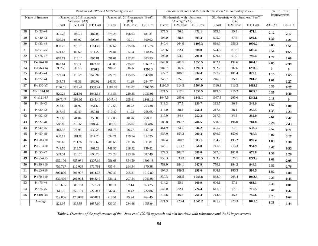
84

Randomised CWS and MCS “safety stocks” Randomised CWS and MCS with robustness “without safety stocks” % E. T. Cost Improvements

Name of Instance (Juan et. al., 2013) approach

“Average” (A3)

(Juan et. al., 2013) approach “Best”.

(B3)

Sim-heuristic with robustness

“Average” (A2)

Sim-heuristic with robustness “Best”.

(B2)

F. cost E.V. Cost E.T. Cost F. cost E.V. Cost E.T. Cost F. cost E.V. Cost E.T. Cost F. cost E.V. Cost E.T. Cost A3—A2 B3—B2

28 E-n22-k4 375.28 106.77 482.05 375.28 106.03 481.31

375.3 96.9 472.1 375.3 95.8 471.1 2.12 2.17

29 E-n30-k3 505.01 95.97 600.98 505.01 95.01 600.02

505.0 88.3 593.3 505.0 87.6 592.6 1.30 1.25

30 E-n33-k4 837.73 276.76 1114.49 837.67 275.06 1112.74

840.4 264.9 1105.3 839.9 256.3 1096.2 0.83 1.51

31 E-n51-k5 524.68 86.60 611.27 524.81 85.54 610.35

525.6 82.4 608.0 524.6 81.8 606.4 0.54 0.65

32 E-n76-k7 692.71 113.10 805.81 691.01 112.52 803.53

698.0 93.7 791.8 699.4 91.0 790.4 1.77 1.66

33 E-n76-k10 842.64 229.36 1072.00 843.86 225.87 1069.73

849.0 201.5 1050.5 852.1 192.6 1044.8 2.05 2.39

34 E-n76-k14 982.7 307.6 1290.3 982.7 307.6 1290.3 982.7 307.6 1290.3 982.7 307.6 1290.3 0 0

35 F-n45-k4 727.74 116.23 843.97 727.75 115.05 842.80

727.7 106.7 834.4 727.7 101.4 829.1 1.15 1.65

36 F-n72-k4 244.71 41.31 286.02 243.50 41.28 284.77

245.7 35.8 281.5 246.0 35.2 281.2 1.61 1.27

37 F-n135-k7 1186.01 323.42 1509.44 1182.33 321.02 1503.35

1190.6 314.3 1504.9 1186.1 313.2 1499.3 0.30 0.27

38 M-n101-k10 820.28 221.91 1042.18 819.56 220.35 1039.91

821.5 217.1 1038.5 819.6 216.2 1035.8 0.35 0.40

39 M-n121-k7 1047.47 298.02 1345.49 1047.49 295.61 1343.10

1047.5 295.6 1343.1 1047.5 295.6 1343.1 0.18 0

40 P-n19-k2 212.66 41.97 254.63 212.66 40.72 253.38

213.2 37.5 250.7 212.7 36.3 248.9 1.57 1.80

41 P-n20-k2 217.42 42.40 259.81 217.42 41.23 258.65

218.0 38.4 256.4 217.4 38.1 255.5 1.33 1.23

42 P-n22-k2 217.86 41.04 258.89 217.85 40.26 258.11

217.9 34.4 252.3 217.9 34.2 252.0 2.61 2.42

43 P-n22-k8 588.80 215.63 804.42 588.79 215.07 803.86

588.8 197.7 786.5 588.8 196.0 784.8 2.28 2.43

44 P-n40-k5 462.33 76.93 539.25 461.73 76.27 537.10

461.9 74.2 536.2 461.7 71.6 533.3 0.57 0.71

45 P-n50-k8 633.17 181.03 814.20 632.71 179.54 812.25

636.9 153.3 790.3 636.7 150.6 787.3 3.02 3.17

46 P-n50-k10 700.66 211.97 912.62 700.66 211.16 911.81

702.4 200.7 903.1 704.2 195.2 899.4 1.05 1.38

47 P-n51-k10 741.50 219.79 961.28 741.50 218.32 959.82

743.1 213.7 956.8 741.5 213.3 954.9 0.47 0.52

48 P-n55-k7 574.54 116.20 690.75 574.23 113.26 687.49

577.3 102.7 680.0 577.0 101.8 678.8 1.58 1.28

49 P-n55-k15 952.106 355.081 1307.19 951.68 354.50 1306.18

953.3 333.3 1286.5 953.7 326.1 1279.9 1.61 2.05

50 P-n60-k10 756.787 215.005 971.792 755.44 214.94 970.38

753.9 194.1 947.9 750.1 194.2 944.3 2.52 2.76

51 P-n65-k10 807.876 206.907 1014.78 807.49 205.31 1012.80

807.3 189.3 996.6 808.1 186.3 994.5 1.82 1.84

52 P-n70-k10 839.496 208.964 1048.46 839.11 207.84 1046.95

839.3 206.5 1045.8 838.9 203.4 1042.3 0.25 0.45

53 P-n76-k4 613.605 58.5163 672.121 606.11 57.14 663.25

614.2 55.6 669.9 606.1 57.1 663.3 0.33 0.01

54 P-n76-k5 641.8 85.5101 727.311 642.43 80.42 722.86

642.0 82.4 724.4 641.9 77.5 719.5 0.40 0.47

55 P-n101-k4 719.066 47.8048 766.871 718.51 45.94 764.45

715.6 45.7 761.3 713.8 45.8 759.6 0.73 0.64

Average 821.05 236.56 1057.60 820.39 234.66 1055.04

821.9 223.4 1045.2 821.2 220.3 1041.5 1.28 1.44

Table 4. Overview of the performance of the “Juan et al. (2013) approach and sim-heuristic with robustness and the % improvements

85

Average costs are presented in Tables 1, 2, 3 and 4 for 55 instances. The row entitled as

‘average’ computes the average of the 55 rows above it for the three approaches namely,

(Juan et al., 2013) approach and sim-heuristic without robustness. Here are some

observations about the average computational costs for all instances: the average cost

obtained by sim-heuristic with robustness achieved better cost compared to sim-heuristic

without robustness, whereas the average cost obtained by (Juan et al., 2013) has a better

cost compared with sim-heuristic without robustness. However, the average cost obtained

by sim-heuristic with robustness has achieved better average cost compared with the

average cost obtained by (Juan et al., 2013). Notice that our approach outperformance all

the approaches. Additionally, the tables also showed the % improvement between the

solutions obtained by these three approaches. Positive % improvement values imply that

the expected total costs obtained with sim-heuristic with robustness is lower (and therefore

better) than the expected total costs obtained with either sim-heuristic without robustness

or (Juan et al. 2013) approach.

A close analysis of the solutions showed that sim-heuristic with robustness provides one

of the best solution approaches, and that the main benefit of the robust solution is that it

has the ability to redistribute the unused vehicle capacity efficiently. If a vehicle does not

have enough capacity for serving a possible demand assigned to it, in the robust solution,

the nearby vehicles with enough capacity are routed in a different way to cover the un-

served demand, with only a slight cost increase. In the case that the vehicle with enough

capacity is far from the un-served customer’s demand, then the robust solution will look

for another vehicle, which has enough capacity in order to meet this demand with a lower

cost.

§3.6 Conclusion

This chapter focused on presenting the robust routing model and sim-heuristic in order to

address the VRPSD with known probability distribution. In this chapter, we have proposed

the robust routing model and the sim-heuristic algorithm that combines the randomised

CWS algorithm with MCS to solve the VRPSD with efficient routing solutions, where the

86

aim of the objective function is to minimise the expected total cost. One of the basic ideas

of our methodology is to take into account the entire capacity of the vehicle without using

the safety stocks, and try to use the robust routing model in order to achieve a robust

solution for VRPSD instances. The model and the algorithm are tested on a large number

of CVRP instances that are converted into stochastic instances. We presented

computational results performed on a set of instances from the literature. These

computational results clearly showed that, the robust routing model generated a good

quality solution for almost all instances. In addition, the computational results have shown

that the sim-heuristic and the robust routing model are effective and efficient in all 55

instances. This is major progress when compared to previous studies on the VRPSD.

We have compared the robust solutions with other solutions in the VRPSD literature to

find the best solution in terms of the minimum expected total costs. Moreover, the robust

routing model satisfies all the customer demands at the same cost as the recourse model,

because the robust routing model sends vehicles amongst customers to satisfy all possible

demands. Among the special characteristics of this approach it is important to highlight

that it has provided competitive solutions to most small and medium-tested instances, that

it does not need any complex fine-tuning process and that it does assume any particular

probability distribution for modelling customers' demands. Also, in all instances, the

proposed approach and robust routing model have produced a feasible/better solution

compared with the other methods in the literature. In the next chapter, we will apply the

robust routing model with a new algorithm which combined randomised IG algorithm with

MCS.

87

Chapter 4 : Sim-Randomised Iterated Greedy

(IG) algorithm to solve Robust VRPSD

§4.1 Introduction

Iterated Greedy (IG) algorithm is a heuristic that has been developed by (Ruiz and Stutzle,

2007) to solve the flowshop scheduling problem with the aim of minimising the makespan.

They stated that the IG algorithm is easily adaptable to other flowshop problems, very

simple to code and parameter free. As a result, IG is very effective and they achieved new

best solutions for Permutation Flowshop Scheduling Problem (PFSP) instances. Ribas et

al. (2011) proposed an IG algorithm in order to solve the blocking flowshop scheduling

problem. Furthermore, it showed an improved Nawaz Enscore Ham (NEH)-based heuristic

by Nawaz et al. (1983) which is used as the initial solution procedure for IG algorithm.

The aim of choosing this method is that IG has been applied successfully for many

Combinatorial Optimisation Problems (COPs) such as the flowshop scheduling problem.

However, it has not been applied to solve VRPSD or even the deterministic case. Also, the

IG algorithm, despite its simplicity, is very competitive as is the case of most efficient

heuristics. The IG algorithm is closely related to the Iterated Local Search (ILS) approach

to provide a solution for COPs by iterating over a greedy constructive heuristic. The central

difference between these two methods is that ILS applies local search to perturbations of

the current search point, to extend the search space and to escape from deep local optima,

whereas IG algorithm considers is a constructive greedy approach with two phases,

destruction and construction. As result, the IG algorithm is more appropriate than ILS to

escape from strong local optima. In terms of the experiments, the IG algorithm was

implemented to scheduling problems and the computational results showed it has great

promise. In fact, the general performance of the IG algorithm can be regarded as very good

since it does not make use of problem specific knowledge like the critical paths concept or

extensive speed-ups, as used in other published heuristics. This chapter is organised as

follows. In Section 4.2, we have provided a brief literature review on the IG algorithm.

88

Section 4.3 gave details about the contribution of the chapter. Section 4.4 gave a detailed

description of the Randomised IG algorithm with MCS. In Section 4.5, we presented a

complete comparative evaluation of the effectiveness and efficiency of the proposed IG

algorithm as well as a comparison to some of the best known solutions approaches.

Conclusions are presented in Section 4.6.

§4.2 Literature review of Iterated Greedy (IG) algorithm

IG algorithm is one of the most significant heuristics method that can deal with scheduling

problems. IG algorithm has been implemented to solve the flow-shop problem combined

with other methods, and the computational results showed its performance. Ruiz and

Stutzle (2005); Ruiz and Stutzle (2007) proposed an IG algorithm to solve different aspects

of the flow-shop problem. For instance, proposing two new IG algorithms for solving a

complex flow-shop problem by minimising the total weighted tardiness and minimising

the maximum completion time. The fundamental concept behind using an IG algorithm is

to iterate over constructive algorithms and the fundamental concept behind using ILS is

that it resides in iterating over local searches in a particular way. Adding ILS into an IG

algorithm can make the similarities between these algorithms become more pronounced.

Ruiz and Stutzle (2005) proposed an IG algorithm to achieve a solution for the flow-shop

problem with sequence dependent setup times, whereby the setup time depends on the job

previously processed on each machine. Also, the ability of the proposed IG algorithm in

finding feasible solutions within reasonable computational times which are near to the

optimum solutions, make it justifiable to use in the flowshop problem with sequence

dependent setup times. A simple and effective IG algorithm based on an NEH constructive

heuristic has been implemented by Ruiz and Stutzle (2007) to solve the PFSP. Also, both

IG algorithm with and without ILS obtained good solutions. They provided a complete

comparative evaluation of the effectiveness and efficiency of this method. A general

pseudo-code of the IG algorithm is given in Figure 12 where the initial sequence of

customers is represented as 𝜋0. 𝜋1 represents the cost of the procedure for both destruction

and construction phases. Finally, 𝜋𝑏𝑒𝑠𝑡 is the sequence of the best solution of the customer

and 𝑑 is the set of customers that are selected randomly.

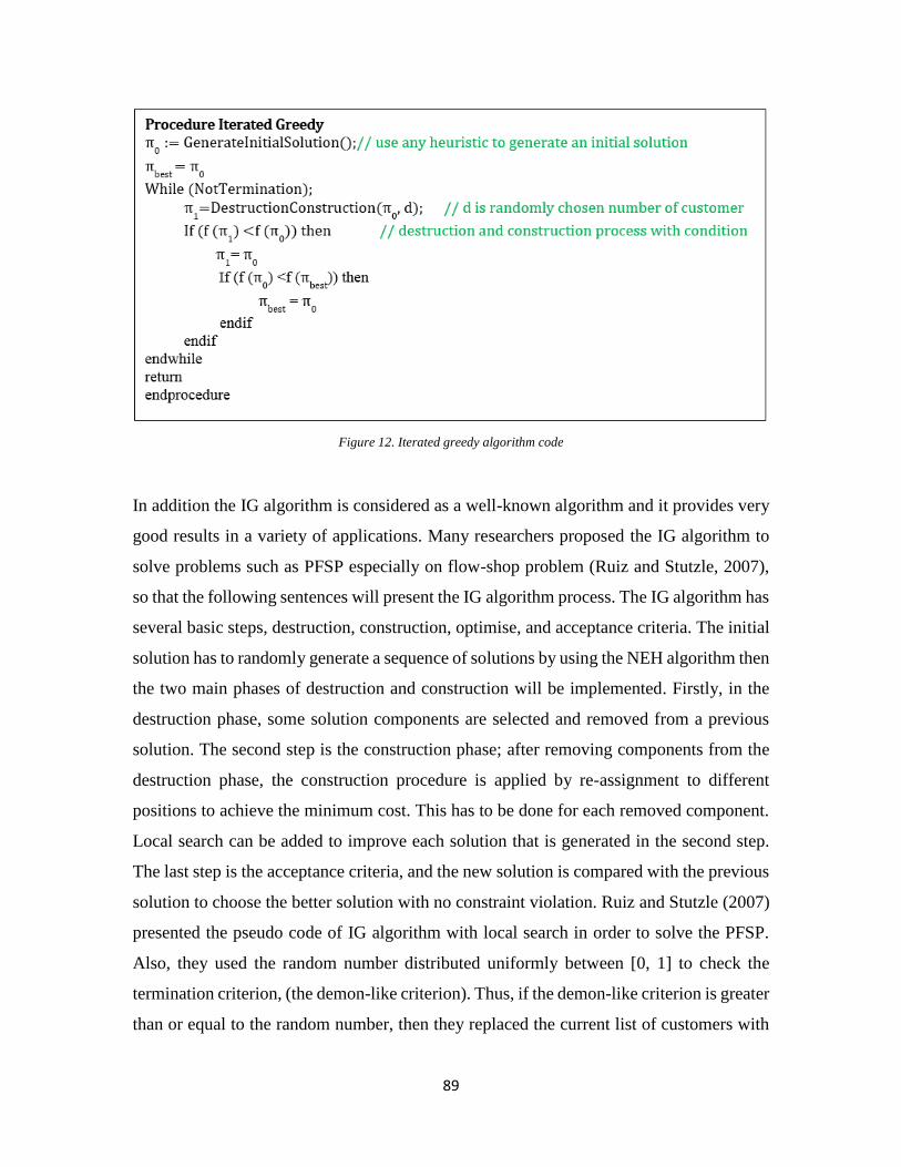
89

Figure 12. Iterated greedy algorithm code

In addition the IG algorithm is considered as a well-known algorithm and it provides very

good results in a variety of applications. Many researchers proposed the IG algorithm to

solve problems such as PFSP especially on flow-shop problem (Ruiz and Stutzle, 2007),

so that the following sentences will present the IG algorithm process. The IG algorithm has

several basic steps, destruction, construction, optimise, and acceptance criteria. The initial

solution has to randomly generate a sequence of solutions by using the NEH algorithm then

the two main phases of destruction and construction will be implemented. Firstly, in the

destruction phase, some solution components are selected and removed from a previous

solution. The second step is the construction phase; after removing components from the

destruction phase, the construction procedure is applied by re-assignment to different

positions to achieve the minimum cost. This has to be done for each removed component.

Local search can be added to improve each solution that is generated in the second step.

The last step is the acceptance criteria, and the new solution is compared with the previous

solution to choose the better solution with no constraint violation. Ruiz and Stutzle (2007)

presented the pseudo code of IG algorithm with local search in order to solve the PFSP.

Also, they used the random number distributed uniformly between [0, 1] to check the

termination criterion, (the demon-like criterion). Thus, if the demon-like criterion is greater

than or equal to the random number, then they replaced the current list of customers with

90

the old one. They also showed the code implementation of an iterative improvement

procedure using the insertion neighbourhood algorithm.

Some researchers have integrated an IG algorithm with other methods in order to solve the

scheduling problems. For example, unrelated parallel machine scheduling solved by using

an IG algorithm based metaheuristic that is able to find good quality solutions in a very

short time (Fanjul-Peyro and Ruiz, 2010). The aim was to minimise the maximum

completion time of the jobs. A variable neighbourhood descent algorithm is used to obtain

an initial solution and it applied Insertion and Interchange local searches till local optimum

is achieved. After that, IG algorithm is implemented to improve the solution. From the

computational results discussion, they are able to select the jobs and machines in a smart

way to achieve one of the good solutions. A comprehensive benchmark test of 1400

instances was tested in order to compare all proposed algorithms against state-of-the-art

methodologies. Also, computational results showed that these solutions are, most of the

time, better than the current state-of-the-art methodologies, by a statistically significant

margin.

Hajer and Talel (2013) presented two variants of both ILS and IG algorithm to minimise

the completion time in two machines PFSP. They also provided a new priority rule based

on the availability of two machines for the total completion time under time lag. Later, IG

algorithm has been combined with simulated annealing by Chalghoumi and Ladhari (2015)

to minimise the total completion time for the two machine flow-shop scheduling problem.

The advantages of these two methods are that it is easy to deal with during the

implementation and it also provides a compromise between intensification and

diversification that improves the solution quality by accepting better solutions. They used

simulated annealing to generate initial solutions then they used IG to obtain the goal. The

characteristic of this method is that it can accept the solutions that improve the current

solution and also accept solutions that deteriorate the current solution. The idea behind IG

is to generate a sequence of solutions and then choose the best solution.

The IG algorithm was proposed to solve different problems and it has shown to reach

excellent performance on the permutation flow-shop problem with different criterion such

91

as time dependence. Furthermore, it is able to improve some of the best known solutions

on the permutation flow-shop problem. A large number of scheduling problems can benefit

from ideas underlying IG algorithm. Mohan and Gopalan (2014) proposed a modified

version of IG algorithm to minimise the total cost along with duration of convergence for

task assignment problem. Also it capitalises on the efficacy of the Parallel Processing

paradigm. The main target of the modification is summarised as follow: (1) to enhance the

quality of assignment in every iteration, (2) to utilise the values from the preceding

iterations and (3) at the same time assigning these smaller computations to internal

processors to hasten the computation. Naderi et al. (2014) proposed a new way:

multiobjectives IG algorithm to solve track scheduling in cross-dock problems with

temporary storage. For this problem a multiobjectives IG algorithm employs advanced

features such as modified crowding selection, restart phase and local search. From the

performance point of view, this proposed method showed better solutions and

outperformed the other methods. Multiobjectives IG algorithm can deal with a population

of non-dominated outcomes as a working set instead of just a single outcome. The IG

algorithm developed by Pranzo and Pacciarelli (2015) to solve a job scheduling problem

with zero buffer constraints and with two known variants, the block job shop scheduling

with swap and without swap. A comparison with recent published results showed that an

IG algorithm improved the best known solutions in a literature review on benchmark

instances. From the computational results, it is also important to notice that the IG has a

broad applicability since it can be easily applied to any complex scheduling problem

modelled by means of the alternative graph formulation.

IG algorithm can be proposed to solve other problems such as flexible flow lines with

sequence dependent step-up times to minimise total weighted completion time (Tkacenko

and Vaidyanathan, 2006), to solve the FIR paraunitary approximation problem (Naderi et

al., 2009) and to solve Market segmentation problem with multiple attributes (Huerta-

Muñoz et al., 2012). In general the IG algorithm has been implemented with success on

different applications such as the Set Cover Problem (SCP) (Chandu, 2015). Despite the

massive research effort on the VRP and the success of using IG in some COPs, there has

not been any published paper on the use of IG algorithm to solve the VRP and its variants

92

especially in VRPSD. For these reasons, this algorithm has special attention in order to

implement IG algorithm on VRPSD.

§4.3 Contribution

In recent years, many algorithms have emerged to address problems such as scheduling

and transportation to obtain better solutions. To the best of our knowledge, there is no

research reported in the literature that implements IG algorithm to solve the VRPSD. IG

algorithm has been successfully applied to solve the scheduling problems, especially PFSP

(Ruiz and Stutzle, 2007). Therefore, the main contribution of the work carried out in this

chapter is to apply randomised IG with MCS to solve VRPSD in order to minimise the

expected total cost. The target is to minimise deviation from the a-priori route and also to

provide a near-optimal solution for the VRPSD using this approach. The methodology

includes two stages: in the first stage, optimal a-priori routes are generated. In the second

stage, the decision maker has to serve all customers’ demands by applying randomised IG

algorithm with MCS, in order to minimise the sum of the expected total cost in all routes.

Note that a 100% of the vehicle maximum capacity is considered during the design stage

and when a vehicle capacity is exceeded, recourse actions have to be planned/ designed to

make sure the feasibility of solutions in case of route failure.

The basic IG algorithm includes two phases. These two phases are the destruction phase,

were several customers are chosen from the incumbent solution, and the construction

phase, were the chosen customers are inserted into the sequence until the stopping criteria

are met. The IG algorithm is remarkably simple, parameter free and iteratively applies

constructive heuristics to the current solution and uses an acceptance criterion to decide

whether the new constructed solution should replace the current one. Also, IG is closely

related to other stochastic local search algorithms and the IG algorithm is able to iterate in

an analogous way over greedy construction heuristics. IG algorithm obtains outstanding

results in terms of accuracy and speed. In this chapter, we used the robust routing model

with the constraints from the previous chapter and we adapt IG for solving VRPSD. MCS

is integrated with randomised version of IG to solve VRPSD. This algorithm requires

93

several steps; an initial solution generated by using CWS and a biased randomised function

(geometric distribution), for sorting the customer demand depending on the probability.

Finally it generates random variables to estimate the expected total cost by using MCS.

The objective function is to minimise the overall transportation cost and it is defined in the

robust routing model with constraints, as explained in aforementioned chapter. The target

was to find better solutions for VRPSD and to design experiments to measure performance

with respect to the instances chosen from the literature.

§4.4 Sim-Randomised IG heuristic

The proposed approach considers the entire vehicle capacity while designing the routes.

This is performed by employing a modified version of the IG algorithm introduced by Ruiz

and Stutzle (2007). The main difference between our approach and (Ruiz and Stutzle, 2007)

is that they used IG algorithm to solve the PFSP. However, one of the most distinctive

characteristics in our approach is the hybridisation of MCS within the randomised version

of IG algorithm, to solve a stochastic case of the VRP in order to improve the decision

process and total costs. As it will be explained later with more detail, in this modified

version the MCS stage is integrated within the randomised IG algorithm, which allows

estimating the variable costs associated with each candidate solution. Thus, among the

multiple solutions generated, the corresponding solutions are compared to each other and

the one with the lowest expected total cost is selected as the best-found routing plan.

The IG algorithm is conceptually simple and works by generating a sequence of solutions

by iterating over a greedy construction heuristic, using two central procedures consisting

of the destruction and the construction phases. In the destruction phase, a number of

solution customers are randomly removed from a previously constructed complete

candidate solution. In this phase, there are two sets 𝜋𝐷and 𝜋𝑅 , where 𝜋𝑅 represents the set

of 𝑑 customers that are selected randomly from a previously destructed complete candidate

solution and 𝜋𝐷 is the set of the remaining customers. The result of these two main phases

are two subsequences, the first being the partial sequence 𝜋𝐷 has size 𝑛 − 𝑑 of customers

after removing 𝑑 customers. The second being a sequence of 𝑑 customers which we denote

as 𝜋𝑅. 𝜋𝑅contains the customers who have to be reinserted into 𝜋𝐷. The construction phase

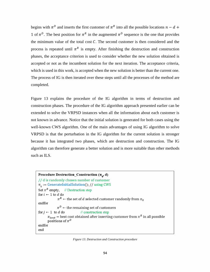
94

begins with 𝜋𝐷 and inserts the first customer of 𝜋𝑅 into all the possible locations 𝑛 − 𝑑 +

1 of 𝜋𝐷. The best position for 𝜋𝑅 in the augmented 𝜋𝐷 sequence is the one that provides

the minimum value of the total cost 𝐶. The second customer is then considered and the

process is repeated until 𝜋𝑅 is empty. After finishing the destruction and construction

phases, the acceptance criterion is used to consider whether the new solution obtained is

accepted or not as the incumbent solution for the next iteration. The acceptance criteria,

which is used in this work, is accepted when the new solution is better than the current one.

The process of IG is then iterated over these steps until all the processes of the method are

completed.

Figure 13 explains the procedure of the IG algorithm in terms of destruction and

construction phases. The procedure of the IG algorithm approach presented earlier can be

extended to solve the VRPSD instances when all the information about each customer is

not known in advance. Notice that the initial solution is generated for both cases using the

well-known CWS algorithm. One of the main advantages of using IG algorithm to solve

VRPSD is that the perturbation in the IG algorithm for the current solution is stronger

because it has integrated two phases, which are destruction and construction. The IG

algorithm can therefore generate a better solution and is more suitable than other methods

such as ILS.

Figure 13. Destruction and Construction procedure

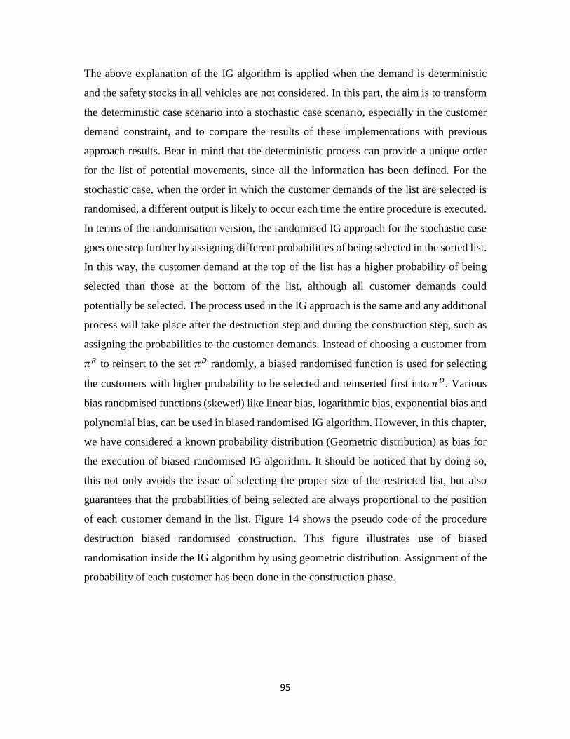
95

The above explanation of the IG algorithm is applied when the demand is deterministic

and the safety stocks in all vehicles are not considered. In this part, the aim is to transform

the deterministic case scenario into a stochastic case scenario, especially in the customer

demand constraint, and to compare the results of these implementations with previous

approach results. Bear in mind that the deterministic process can provide a unique order

for the list of potential movements, since all the information has been defined. For the

stochastic case, when the order in which the customer demands of the list are selected is

randomised, a different output is likely to occur each time the entire procedure is executed.

In terms of the randomisation version, the randomised IG approach for the stochastic case

goes one step further by assigning different probabilities of being selected in the sorted list.

In this way, the customer demand at the top of the list has a higher probability of being

selected than those at the bottom of the list, although all customer demands could

potentially be selected. The process used in the IG approach is the same and any additional

process will take place after the destruction step and during the construction step, such as

assigning the probabilities to the customer demands. Instead of choosing a customer from

𝜋𝑅 to reinsert to the set 𝜋𝐷 randomly, a biased randomised function is used for selecting

the customers with higher probability to be selected and reinserted first into 𝜋𝐷. Various

bias randomised functions (skewed) like linear bias, logarithmic bias, exponential bias and

polynomial bias, can be used in biased randomised IG algorithm. However, in this chapter,

we have considered a known probability distribution (Geometric distribution) as bias for

the execution of biased randomised IG algorithm. It should be noticed that by doing so,

this not only avoids the issue of selecting the proper size of the restricted list, but also

guarantees that the probabilities of being selected are always proportional to the position

of each customer demand in the list. Figure 14 shows the pseudo code of the procedure

destruction biased randomised construction. This figure illustrates use of biased

randomisation inside the IG algorithm by using geometric distribution. Assignment of the

probability of each customer has been done in the construction phase.

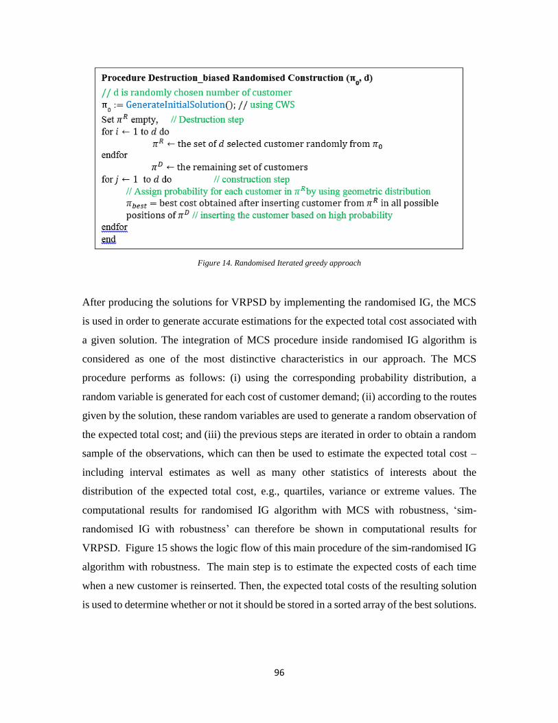
96

Figure 14. Randomised Iterated greedy approach

After producing the solutions for VRPSD by implementing the randomised IG, the MCS

is used in order to generate accurate estimations for the expected total cost associated with

a given solution. The integration of MCS procedure inside randomised IG algorithm is

considered as one of the most distinctive characteristics in our approach. The MCS

procedure performs as follows: (i) using the corresponding probability distribution, a

random variable is generated for each cost of customer demand; (ii) according to the routes

given by the solution, these random variables are used to generate a random observation of

the expected total cost; and (iii) the previous steps are iterated in order to obtain a random

sample of the observations, which can then be used to estimate the expected total cost –

including interval estimates as well as many other statistics of interests about the

distribution of the expected total cost, e.g., quartiles, variance or extreme values. The

computational results for randomised IG algorithm with MCS with robustness, ‘sim-

randomised IG with robustness’ can therefore be shown in computational results for

VRPSD. Figure 15 shows the logic flow of this main procedure of the sim-randomised IG

algorithm with robustness. The main step is to estimate the expected costs of each time

when a new customer is reinserted. Then, the expected total costs of the resulting solution

is used to determine whether or not it should be stored in a sorted array of the best solutions.

97

Figure 15. Randomised Iterated greedy approach with MCS

In general, we provided an example of how the IG algorithm might work: if someone was

asked to plan a route showing the shortest distance a vehicle could drive from one location

to another, he or she would be likely to select the shortest roads. An example of the

application of one iteration of the IG algorithm without local search is given below in figure

16, in order to illustrate the function and procedures of the IG algorithm and the concept

of this algorithm. The example has three vehicles to serve 13 customers, and starts from

the initial solutions. It is assumed that the initial solution will be similar for all the vehicles:

Vehicle 1 serves Customers 13, 3, 6, 2, 4 and 12, Vehicle 2 serves Customers 1, 11 and 8,

and the final vehicle serves Customers 7, 10, 5 and 9. This study focuses on Vehicle 1 and

implements only one iteration of the IG algorithm. Two customers (3 and 4) are then

selected at random from the original solution before reinserting the customers in different

positions, calculating the cost and comparing it with the previous cost.

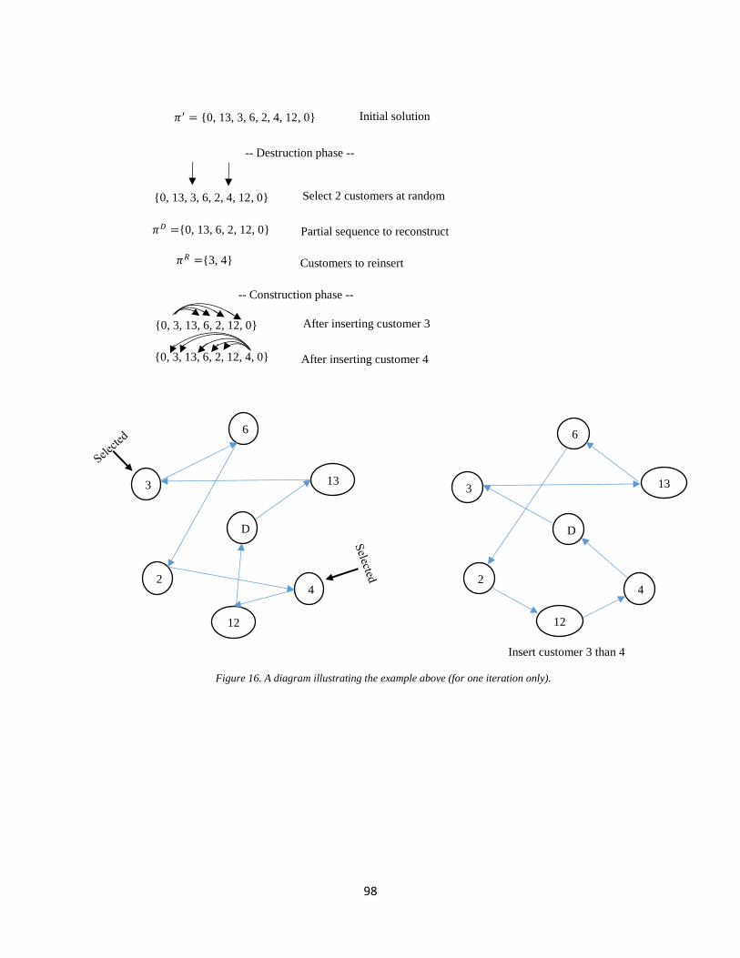
98

𝜋′ = {0, 13, 3, 6, 2, 4, 12, 0} Initial solution

-- Destruction phase --

{0, 13, 3, 6, 2, 4, 12, 0} Select 2 customers at random

𝜋𝐷 ={0, 13, 6, 2, 12, 0}

𝜋𝑅 ={3, 4}

Partial sequence to reconstruct

Customers to reinsert

-- Construction phase --

{0, 3, 13, 6, 2, 12, 0} After inserting customer 3

{0, 3, 13, 6, 2, 12, 4, 0} After inserting customer 4

12

4 2

3

6

13

D

12

4 2

3

6

13

D

Insert customer 3 than 4

Figure 16. A diagram illustrating the example above (for one iteration only).

99

§4.5 Computational results

In the experiments conducted, we tested the performance of a sim-randomised IG algorithm

with robustness on the same instances and also we used the % improvement equation that

has been explained in more detail in section 3.6 for VRPSD. In this chapter, we provided

comprehensive computational results in terms of the average and best that are shown in the

tables 5, 6, 7 and 8, which consist of selecting some of the largest VRPSD instances. Tables

5 and 6 showed the comparison between the results achieved for all 55 instances with

different customers and vehicles. The tables below clearly showed the computational

results obtained by two approaches namely: sim-heuristic with robustness and sim-

randomised IG algorithm with robustness, in terms of the average solution costs. Then, we

compared the performance of this approach against the best performing solution for sim-

heuristic with robustness. The columns ‘sim-randomised IG algorithm with robustness’

summarised the average results obtained by applying sim-randomised IG algorithm with

robustness. The columns ‘sim-heuristic with robustness’ summarised the average obtained

by applying the proposed sim-heuristic with robustness.

Our results for each instance in this chapter can be compared with the aforementioned best

known solutions of the previous chapter. Notice that fixed costs in column 3 which were

obtained by sim-heuristic with robustness, are always lower or equal to those in column 6

which were obtained by sim-randomised IG algorithm with robustness. There are three

instances that are equal to each other in terms of fixed costs which are A-n33-k6, A-n37-

k5 and P-n22-k2. In terms of the expected variable costs, there are 15 instances where the

solutions obtained by sim-randomised IG algorithm with robustness are lower than the

solutions obtained by sim-heuristic with robustness. However, there are 39 instances where

the solutions obtained by sim-heuristic with robustness are lower than the solutions

obtained by sim-randomised IG algorithm with robustness. One instance, P-n50-k8, has

the same expected variable costs. Also the expected total cost solutions in column 5 which

were obtained by sim-heuristic with robustness are always lower than those in column 8

which were obtained by sim-randomised IG algorithm with robustness. Additionally,

Tables 5 and 6 showed the improvements between expected total costs obtained using sim-

100

heuristic with robustness and expected total costs obtained using sim-randomised IG

algorithm with robustness.

These % E. T. Cost improvement are shown in the last column of the tables. It can be

deduced that the performance of sim-heuristic with robustness approach produced better

results than the performance of the sim-randomised IG algorithm with robustness, in

average results as shown in the tables 5 and 6. In addition, the average value of the results

for each approach for all instances is equal to 1.23%. Based on the obtained average of

quality solutions in each approach, we can conclude that the average solution by the

aforementioned approach showed better results than the approach which was presented in

this chapter. In addition, the most interesting result is that in most cases these %

improvements are small, such as the smallest % improvement is A-n38-k5 which has been

improved by 0.15%. Also, sometimes these % improvements can be higher e.g. B-n56-k7,

E-n76-k14, F-n135-k7 and P-n101-k4. From table 3 and 4, in terms of the % improvement

column, in 27 out of 55 instances the % improvement of the expected total cost is less than

1%, in 26 out of 55 it is between 1% to 3% and in 2 out of 55 instances is more than 3%.

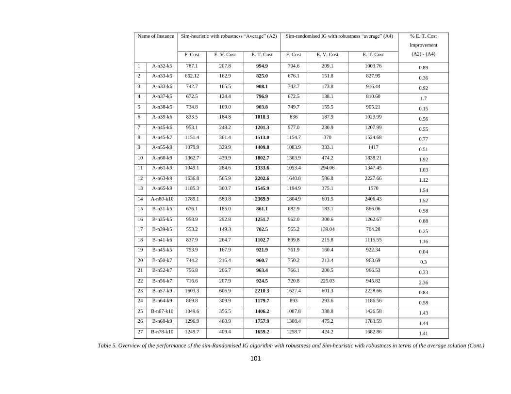
101

Name of Instance Sim-heuristic with robustness “Average” (A2) Sim-randomised IG with robustness “average” (A4) % E. T. Cost

Improvement

(A2) - (A4) F. Cost E. V. Cost E. T. Cost F. Cost E. V. Cost E. T. Cost

1 A-n32-k5 787.1 207.8 994.9 794.6 209.1 1003.76 0.89

2 A-n33-k5 662.12 162.9 825.0 676.1 151.8 827.95 0.36

3 A-n33-k6 742.7 165.5 908.1 742.7 173.8 916.44 0.92

4 A-n37-k5 672.5 124.4 796.9 672.5 138.1 810.60 1.7

5 A-n38-k5 734.8 169.0 903.8 749.7 155.5 905.21 0.15

6 A-n39-k6 833.5 184.8 1018.3 836 187.9 1023.99 0.56

7 A-n45-k6 953.1 248.2 1201.3 977.0 230.9 1207.99 0.55

8 A-n45-k7 1151.4 361.4 1513.0 1154.7 370 1524.68 0.77

9 A-n55-k9 1079.9 329.9 1409.8 1083.9 333.1 1417 0.51

10 A-n60-k9 1362.7 439.9 1802.7 1363.9 474.2 1838.21 1.92

11 A-n61-k9 1049.1 284.6 1333.6 1053.4 294.06 1347.45 1.03

12 A-n63-k9 1636.8 565.9 2202.6 1640.8 586.8 2227.66 1.12

13 A-n65-k9 1185.3 360.7 1545.9 1194.9 375.1 1570 1.54

14 A-n80-k10 1789.1 580.8 2369.9 1804.9 601.5 2406.43 1.52

15 B-n31-k5 676.1 185.0 861.1 682.9 183.1 866.06 0.58

16 B-n35-k5 958.9 292.8 1251.7 962.0 300.6 1262.67 0.88

17 B-n39-k5 553.2 149.3 702.5 565.2 139.04 704.28 0.25

18 B-n41-k6 837.9 264.7 1102.7 899.8 215.8 1115.55 1.16

19 B-n45-k5 753.9 167.9 921.9 761.9 160.4 922.34 0.04

20 B-n50-k7 744.2 216.4 960.7 750.2 213.4 963.69 0.3

21 B-n52-k7 756.8 206.7 963.4 766.1 200.5 966.53 0.33

22 B-n56-k7 716.6 207.9 924.5 720.8 225.03 945.82 2.36

23 B-n57-k9 1603.3 606.9 2210.3 1627.4 601.3 2228.66 0.83

24 B-n64-k9 869.8 309.9 1179.7 893 293.6 1186.56 0.58

25 B-n67-k10 1049.6 356.5 1406.2 1087.8 338.8 1426.58 1.43

26 B-n68-k9 1296.9 460.9 1757.9 1308.4 475.2 1783.59 1.44

27 B-n78-k10 1249.7 409.4 1659.2 1258.7 424.2 1682.86 1.41

Table 5. Overview of the performance of the sim-Randomised IG algorithm with robustness and Sim-heuristic with robustness in terms of the average solution (Cont.)

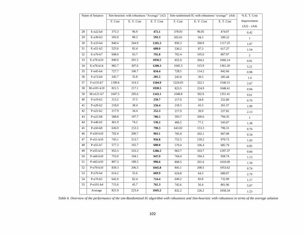
102

Name of Instance Sim-heuristic with robustness “Average” (A2) Sim-randomised IG with robustness “average” (A4) % E. T. Cost

Improvement

(A2) – (A4)

F. Cost E. V. Cost E. T. Cost F. Cost E. V. Cost E. T. Cost

28 E-n22-k4 375.3 96.9 472.1 378.03 96.05 474.07 0.42

29 E-n30-k3 505.0 88.3 593.3 505.01 94.3 599.32 1

30 E-n33-k4 840.4 264.9 1105.3 856.3 260.9 1117.25 1.07

31 E-n51-k5 525.6 82.4 608.0 530.2 87.3 617.27 1.54

32 E-n76-k7 698.0 93.7 791.8 702.4 105.6 807.97 2

33 E-n76-k10 849.0 201.5 1050.5 855.9 204.2 1060.14 0.91

34 E-n76-k14 982.7 307.6 1290.3 1045.3 315.9 1361.20 5.21

35 F-n45-k4 727.7 106.7 834.4 728.5 114.2 842.66 0.98

36 F-n72-k4 245.7 35.8 281.5 245.9 39.5 285.44 1.4

37 F-n135-k7 1190.6 314.3 1504.9 1224.03 322.1 1546.15 2.67

38 M-n101-k10 821.5 217.1 1038.5 823.5 224.9 1048.41 0.94

39 M-n121-k7 1047.5 295.6 1343.1 1048.8 302.6 1351.41 0.61

40 P-n19-k2 213.2 37.5 250.7 217.9 34.8 252.80 0.79

41 P-n20-k2 218.0 38.4 256.4 218.3 43.3 261.57 1.99

42 P-n22-k2 217.9 34.4 252.3 217.9 39.9 257.82 2.13

43 P-n22-k8 588.8 197.7 786.5 593.7 200.6 794.35 1

44 P-n40-k5 461.9 74.2 536.2 466.5 77.2 543.67 1.38

45 P-n50-k8 636.9 153.3 790.3 643.02 153.3 796.31 0.76

46 P-n50-k10 702.4 200.7 903.1 705.9 202.1 907.99 0.54

47 P-n51-k10 743.1 213.7 956.8 752.5 218.2 970.73 1.43

48 P-n55-k7 577.3 102.7 680.0 579.4 106.4 685.79 0.85

49 P-n55-k15 953.3 333.3 1286.5 963.7 333.7 1297.37 0.84

50 P-n60-k10 753.9 194.1 947.9 764.4 194.3 958.74 1.13

51 P-n65-k10 807.3 189.3 996.6 808.5 201.6 1010.09 1.34

52 P-n70-k10 839.3 206.5 1045.8 845.1 208.5 1053.62 0.74

53 P-n76-k4 614.2 55.6 669.9 624.8 64.3 689.07 2.79

54 P-n76-k5 642.0 82.4 724.4 649.2 83.8 732.99 1.17

55 P-n101-k4 715.6 45.7 761.3 745.6 56.4 801.96 5.07

Average 821.9 223.4 1045.2 832.2 226.2 1058.34 1.23

Table 6. Overview of the performance of the sim-Randomised IG algorithm with robustness and Sim-heuristic with robustness in terms of the average solution

103

Tables 7 and 8 summarised the best results that were obtained by two approaches namely:

the sim-heuristic with robustness which is presented in columns 3-5 and sim-randomised

IG with robustness which is presented in column 6-8. Also these tables include the %

improvement between these approaches. We reported the cost of the best solution found in

any run of the heuristic. In the mentioned approaches, the best solution is computed in each

instance. It can be deduced that the performance of the sim-heuristic with robustness

produces better results than the performance of the sim-randomised IG with robustness as

shown in the tables. It is necessary to notice that using a sim-randomised IG algorithm with

robustness it is able to increase the expected total cost as shown in the tables 7 and 8. This

is because a vehicle does not have any restrictions and it can travel back when the vehicle

capacity is exceeded, this can lead to an increase in the total expected cost. Also, since no

safety stock is used, there is chance that these solutions can suffer from route failure which

can increase the expected total cost. Therefore, route failure might imply high expected

variable cost.

Using sim-randomised IG algorithm with robustness could improve the expected variable

costs in some instances. Therefore, 17 instance solutions obtained by sim-randomised IG

algorithm with robustness have lower costs than solutions obtained by sim- heuristic with

robustness. The fixed costs in column 3, which is obtained by sim-heuristic with

robustness, are always lower or equal to those in column 6, which is obtained by sim-

randomised IG algorithm with robustness. Whereas, there are 8 instance solutions which

are equal to each other. Also, 4 instances solutions, which are A-n45-k7, A-n80-k10, B-

n64-k9 and E-n76-k7, obtained by sim-heuristic with robustness are less than those

obtained by sim-randomised IG with robustness. The approach proposed in this chapter

seems to provide far from optimal solutions which can be improved by other algorithms.

In addition, the average value of the results for each approach for all instances of the

problem is equal to 0.98%. Therefore, the average solution by the aforementioned

approach, ‘sim-heuristic with robustness’, showed better results than the approach which

was presented in this chapter, ‘sim-randomised IG algorithm with robustness’. Expected

total costs in column 5 which was obtained by sim-heuristic with robustness are always

lower than those in column 8 which was obtained by sim-randomised IG algorithm with

robustness.

104

Tables 7 and 8 show the % E. T. Cost improvements associated with each approach for the

instance. Therefore, in Tables 7 and 8, the %improvements between two discussed

stochastic approaches are presented in the last column. In most instances, results of two

approaches have shown that this % improvement is small, sometimes it can be above 3%

such as E-n76-k14, P-n76-k4 and P-n101-k4. It can be noticed that according to the %

improvement column it is clear that sim-heuristic with robustness always has superior

results to randomised IG algorithm with MCS and robustness. In 2 out of 55 instances the

equality of the solutions is less than 0.1%, in 49 out of 55 instances the equality of the

solutions is between 0.1% to 2% and in 4 out of 55 instances the equality of the solutions

is more than 2%. E-n76-k14, P-n76-k4 and P-n101-k4 achieved the biggest %

improvements which is 5.23, 3.15% and 3.24% respectively. E-n76-k14 showed the

biggest % improvement between sim-heuristic with robustness and the sim-randomised IG

algorithm with robustness as shown in the tables.

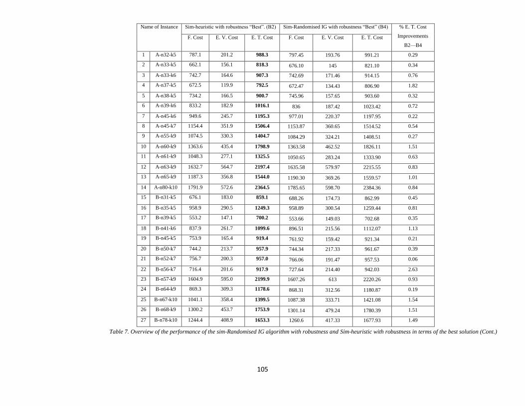
105

Name of Instance Sim-heuristic with robustness “Best”. (B2) Sim-Randomised IG with robustness “Best” (B4) % E. T. Cost

Improvements

B2—B4

F. Cost E. V. Cost E. T. Cost F. Cost E. V. Cost E. T. Cost

1 A-n32-k5 787.1 201.2 988.3 797.45 193.76 991.21 0.29

2 A-n33-k5 662.1 156.1 818.3 676.10 145 821.10 0.34

3 A-n33-k6 742.7 164.6 907.3 742.69 171.46 914.15 0.76

4 A-n37-k5 672.5 119.9 792.5 672.47 134.43 806.90 1.82

5 A-n38-k5 734.2 166.5 900.7 745.96 157.65 903.60 0.32

6 A-n39-k6 833.2 182.9 1016.1 836 187.42 1023.42 0.72

7 A-n45-k6 949.6 245.7 1195.3 977.01 220.37 1197.95 0.22

8 A-n45-k7 1154.4 351.9 1506.4 1153.87 360.65 1514.52 0.54

9 A-n55-k9 1074.5 330.3 1404.7 1084.29 324.21 1408.51 0.27

10 A-n60-k9 1363.6 435.4 1798.9 1363.58 462.52 1826.11 1.51

11 A-n61-k9 1048.3 277.1 1325.5 1050.65 283.24 1333.90 0.63

12 A-n63-k9 1632.7 564.7 2197.4 1635.58 579.97 2215.55 0.83

13 A-n65-k9 1187.3 356.8 1544.0 1190.30 369.26 1559.57 1.01

14 A-n80-k10 1791.9 572.6 2364.5 1785.65 598.70 2384.36 0.84

15 B-n31-k5 676.1 183.0 859.1 688.26 174.73 862.99 0.45

16 B-n35-k5 958.9 290.5 1249.3 958.89 300.54 1259.44 0.81

17 B-n39-k5 553.2 147.1 700.2 553.66 149.03 702.68 0.35

18 B-n41-k6 837.9 261.7 1099.6 896.51 215.56 1112.07 1.13

19 B-n45-k5 753.9 165.4 919.4 761.92 159.42 921.34 0.21

20 B-n50-k7 744.2 213.7 957.9 744.34 217.33 961.67 0.39

21 B-n52-k7 756.7 200.3 957.0 766.06 191.47 957.53 0.06

22 B-n56-k7 716.4 201.6 917.9 727.64 214.40 942.03 2.63

23 B-n57-k9 1604.9 595.0 2199.9 1607.26 613 2220.26 0.93

24 B-n64-k9 869.3 309.3 1178.6 868.31 312.56 1180.87 0.19

25 B-n67-k10 1041.1 358.4 1399.5 1087.38 333.71 1421.08 1.54

26 B-n68-k9 1300.2 453.7 1753.9 1301.14 479.24 1780.39 1.51

27 B-n78-k10 1244.4 408.9 1653.3 1260.6 417.33 1677.93 1.49

Table 7. Overview of the performance of the sim-Randomised IG algorithm with robustness and Sim-heuristic with robustness in terms of the best solution (Cont.)

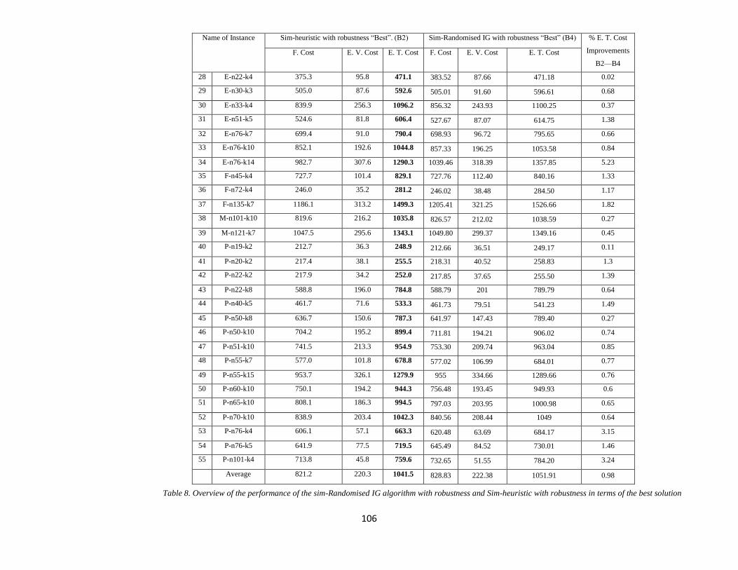
106

Name of Instance Sim-heuristic with robustness “Best”. (B2) Sim-Randomised IG with robustness “Best” (B4) % E. T. Cost

Improvements

B2—B4

F. Cost E. V. Cost E. T. Cost F. Cost E. V. Cost E. T. Cost

28 E-n22-k4 375.3 95.8 471.1 383.52 87.66 471.18 0.02

29 E-n30-k3 505.0 87.6 592.6 505.01 91.60 596.61 0.68

30 E-n33-k4 839.9 256.3 1096.2 856.32 243.93 1100.25 0.37

31 E-n51-k5 524.6 81.8 606.4 527.67 87.07 614.75 1.38

32 E-n76-k7 699.4 91.0 790.4 698.93 96.72 795.65 0.66

33 E-n76-k10 852.1 192.6 1044.8 857.33 196.25 1053.58 0.84

34 E-n76-k14 982.7 307.6 1290.3 1039.46 318.39 1357.85 5.23

35 F-n45-k4 727.7 101.4 829.1 727.76 112.40 840.16 1.33

36 F-n72-k4 246.0 35.2 281.2 246.02 38.48 284.50 1.17

37 F-n135-k7 1186.1 313.2 1499.3 1205.41 321.25 1526.66 1.82

38 M-n101-k10 819.6 216.2 1035.8 826.57 212.02 1038.59 0.27

39 M-n121-k7 1047.5 295.6 1343.1 1049.80 299.37 1349.16 0.45

40 P-n19-k2 212.7 36.3 248.9 212.66 36.51 249.17 0.11

41 P-n20-k2 217.4 38.1 255.5 218.31 40.52 258.83 1.3

42 P-n22-k2 217.9 34.2 252.0 217.85 37.65 255.50 1.39

43 P-n22-k8 588.8 196.0 784.8 588.79 201 789.79 0.64

44 P-n40-k5 461.7 71.6 533.3 461.73 79.51 541.23 1.49

45 P-n50-k8 636.7 150.6 787.3 641.97 147.43 789.40 0.27

46 P-n50-k10 704.2 195.2 899.4 711.81 194.21 906.02 0.74

47 P-n51-k10 741.5 213.3 954.9 753.30 209.74 963.04 0.85

48 P-n55-k7 577.0 101.8 678.8 577.02 106.99 684.01 0.77

49 P-n55-k15 953.7 326.1 1279.9 955 334.66 1289.66 0.76

50 P-n60-k10 750.1 194.2 944.3 756.48 193.45 949.93 0.6

51 P-n65-k10 808.1 186.3 994.5 797.03 203.95 1000.98 0.65

52 P-n70-k10 838.9 203.4 1042.3 840.56 208.44 1049 0.64

53 P-n76-k4 606.1 57.1 663.3 620.48 63.69 684.17 3.15

54 P-n76-k5 641.9 77.5 719.5 645.49 84.52 730.01 1.46

55 P-n101-k4 713.8 45.8 759.6 732.65 51.55 784.20 3.24

Average 821.2 220.3 1041.5 828.83 222.38 1051.91 0.98

Table 8. Overview of the performance of the sim-Randomised IG algorithm with robustness and Sim-heuristic with robustness in terms of the best solution

107

From all tables above, the most % improvements between sim-heuristic with robustness

and sim-randomised IG algorithm with robustness is small in both average and best

solutions. However, sometimes, these % improvements could be higher. It can be observed

that none of the expected total costs of the proposed algorithm outperformed the sim-

heuristic with robustness. Also, we can observe that from Table 5 and 6, the average quality

of the sim-heuristic with robustness is 1045.2, while the average quality of the solution of

the proposed algorithm in this chapter is 1058.34. From Table 7 and 8, the average quality

of the sim-heuristic with robustness is 1041.5, while the average quality of the solution of

the proposed algorithm in this chapter is 1051.91. Thus, the inclusion of several

modifications is necessary for the effectiveness of the proposed algorithm ‘sim-randomised

IG with robustness’.

§4.6 Conclusion

We have extended IG algorithm by using both randomisation and MCS. In this chapter, we

proposed a sim-randomised IG algorithm. We then analysed the trade-offs of these

solutions on instances. The IG algorithm makes use of a destruction phase that randomly

removes a number of customers from the sequence, and a construction phase that reinserts

the previously removed customers to obtain the optimal solutions. Designing IG algorithm

boils down to determining the order in which to consider the customers and figuring out

the suitable solutions. In doing so, this combination between customers is more likely to

improve the obtained solutions. We have applied sim-randomised IG algorithm with

robustness for solving a VRPSD. Sim-randomised IG algorithm with robustness provided

results that were not as good as the randomised parallel version of the CWS algorithm with

MCS ‘sim-heuristic’ with the robust routing model. As shown in the preliminary result

tables it compares two types of results which are sim-heuristic with robustness and sim-

randomised IG algorithm with robustness. We finished the section verifying that the sim-

heuristic with robustness provided better results to the stochastic demand than sim-

randomised IG with robustness. In this chapter, it is significant to notice that results of

these algorithms do not employ any local search process. The local search is not

108

implemented for several reasons. Firstly, the solutions that were achieved by sim-

randomised IG with robustness are not better than the previous solutions which were

obtained by sim-heuristic with robustness. Therefore, when the local search is applied, it

cannot get better solutions than the sim-heuristic with robustness solutions. The second

reason is that biased randomised and simulation have been applied and this is better way

than local search; biased randomised and simulation does not provide good solutions when

compared with the previous solutions. Finally, time is considered to be important and for

this reason the IG algorithm using local search implicitly has been applied in the next

chapter in order to improve the solutions that were obtained by the sim-heuristic with

robustness.

109

Chapter 5 : Sim-heuristic and IG algorithm with

local search to solve robust VRPSD

§5.1 Introduction

Local search can be defined as a heuristic method for solving computationally hard

optimisation problems. In addition, local search algorithms were first proposed several

decades ago and have been shown to exhibit good practical performance in empirical

studies. There are dozens of successful algorithms for the VRP and its variants that

incorporate some form of local search, and feasible solutions that are further improved via

a local search. Many researchers have studied different local search algorithms, such as

simulated annealing, tabu search and genetic algorithm. We listed a few of the better-

known algorithms that employ local search, but our discussion is not intended to be

exhaustive. In addition, there are recent literature reviews (Braysy, and Gendreau, 2005),

(Braysy and Gendreau, 2005a) and (Gendreau, et al., 2008) which highlight examples of

successful local search implementations. They stated that local search algorithms are

considered to be one of the available methods that can obtain good solutions to large

problems. These algorithms are also widely applied to numerous hard computational

problems including those in computer science, mathematics, operational research,

engineering and scheduling.

The aim of using a local search algorithm is to move from one solution to another in the

space of candidate solutions by applying local changes, until a solution is deemed optimal,

is found or a time bound is elapsed. Therefore, two common choices can be used to

terminate the local search steps: it can be based on a time bound, or based on the best

solution found by the algorithm that has not been improved in a given number of steps.

The number of repetitions is a trade-off between the running time of the algorithm and the

solution quality. This chapter is organised as follows. In section 5.2, we provided a

literature review on local search methods. The contribution of this chapter is presented in

section 5.3. We described our methodology in order to improve the solution of VRPSD in

section 5.4. In section 5.5, we provided the results of computational experiments and a

110

comparison to the best known solutions approaches. We concluded with a summary of the

chapter in section 5.6.

§5.2 Literature review on local search

Many researchers are interested in improving heuristic search methods because these are

more generally applicable. The fundamental goal behind this improvement is to help

experts in the design of effective heuristic methods and subsequently to find a better

solution for hard computational problems. Local search has become one of the widely

accepted techniques to solve COPs (Aarts, and Lenstra, (1997). Therefore, local search

algorithms have been proven to be effective at providing good solutions with a low

computational effort to the classical VRP instances, and also to solve additional constraints

such as time windows and multiple depots (Groer et al., 2010). In addition, in terms of the

solution quality of the local search algorithms, they can generate a good solution when a

large number of repetitions is allowed. Choosing an appropriate number of repetitions

depends on the execution and trade-off between the running time and the solution quality.

Therefore, when the data is big, a large number of repetitions should be applied to improve

the result for the algorithm. However, if either the number of times or the data is small, a

small number of repetitions should be applied.

A local search algorithm would improve each solution generated and immediately accepts

a better solution. Several studies have successfully implemented a local search algorithm

to solve the VRP and its variants. Other studies also integrated some form of local search.

Gendreau et al. (2008) provided a good review of recent literature with a categorised

bibliography of the most popular type of metaheuristics to solve VRPs and their extensions,

with additional examples of successful local search implementations. Groer et al. (2010)

presented seven local search operators to quickly generate solutions to solve VRP

instances. These operators improved the solutions with 1% on the best known solution to

the benchmark problems. Very generally, Ibaraki, et al. (2011), a local search can usually

be started with the initialisation method to generate the initial solutions, based upon the

111

given seed from the beginning. Customers can then be inserted into the solution route one

at a time. Data used during the implementation, would include the customer to be inserted,

the distance between the customers, the customers’ demands and which customer was the

most recently inserted. When it is unfeasible to insert any customer into the current route,

due to, for example, a violation of the capacity constraints, a new route solution should be

generated. This procedure is repeated until all customers have been routed and the stopping

criterion is satisfied.

Local search algorithms consider commonly used techniques in COPs. Pop and Horvat-

Marc (2012), Local optimality arises in the context of local search algorithms, which

attempts to improve solutions by considering perturbations of the current solution. The

main idea of using the local search is to start with some feasible solution for the problem

and then improve it. If a better solution is found, then the new solution will be selected and

the same procedure will be repeated. If no solution is better than the current solution, it is

locally optimal and then the process stops. Finding locally optimal solutions is presumably

easier than finding optimal solutions. They considered theoretical aspects of seven

neighbourhoods that were used in the local search approach. In terms of the results, they

investigated all the possible connections of the exchanged vertices within the clusters, to

get improved routes (i.e. the nodes belonging to the marked clusters after the exchange

may be different).

Local search can be applied with different variants of VRP. For example, Savelsbergh,

(1985) used local search algorithms to find better solutions for VRP with Time Windows

(VRPTW) and these algorithms were based on the k-interchange concept. The algorithms

could be solved without increasing the time complexity of the VRPTW. Braysy and

Gendreau (2005) presented a review of research on VRPTW and VRPTW heuristics

generally used to assess the quality of solutions in terms of objective function value and

the speed. They proposed two methods which are the traditional heuristic route

construction method and the recent local search algorithm method, that is, route

construction and route improvement (local search) methods. Another example is an

adaptive local search algorithm that was developed by Avci and Topaloglu (2015) to solve

two variants of the classical VRP, VRP with Simultaneous Pickups and Deliveries

112

(VRPSPD) and VRP with Mixed Pickup and Delivery (VRPMPD). According to the

literature, this algorithm was tested on well-known benchmark instances for both problems.

An advantage of using this algorithm was that it could effectively solve both problems

within a reasonable computational time. Solano-Charris (2015) proposed a mixed integer

linear program, two greedy algorithm heuristics and four local searches based on

metaheuristics to solve CVRP. In addition, by using these approaches, the researcher

sought high quality solutions for a robust VRP with uncertain travel costs.

Several families of VRPs using local search have been introduced. However, local search

algorithms can be applied in the field of COPs such as scheduling, from which several

papers were selected for covering different variants. Flowshop scheduling is an active

research area of considerable interest to researchers. New and better solutions are

achievable using different algorithms for common benchmarks at a rapid pace. Several

recent studies investigating local search have been carried out in different fields such as

manufacturing and flowshop scheduling. Many authors have considered the local search

after building the initial solution. Notably, Ruiz and Stutzle (2007) offered a good example

of the implementation of a local search to a flowshop scheduling problem after applying a

specific heuristic. Three steps were taken to improve solution costs. They used a well-

known heuristic, the NEH, to produce an initial solution and proposed a new IG algorithm

that applies two phases iteratively, namely the destruction and the construction phase. They

then applied a local search after the construction phase to improve the solutions as shown

in their experimental results. Their experimental results included a comparison between

the proposed IG algorithm and other powerful algorithms (state-of-the-art methods) giving

a comprehensive experimental evaluation.

Wang et al. (2011) proposed a hybrid modified global-best harmony search algorithm for

solving the blocking permutation flow shop scheduling problem with the makespan

criterion. They generated the initial solution with higher quality and hybridised the

harmony search algorithm based on a global search and a local search algorithm based on

insert neighbourhood in order to have a good balance between the global exploration and

local exploitation. Moreover, a new pitch adjustment rule is developed to inherit good

structures from the global-best harmony vector. Computational simulations and

113

comparisons demonstrated the superiority of the proposed hybrid harmony search

algorithm, in terms of solution quality and time requirements. Pan and Ruiz (2012)

examined local search methods for the flowshop scheduling problem with flowtime

minimisation. The first two proposed methods are based on the well-known ILS and IG

frameworks which have been successfully applied to other flowshop problems. In addition,

they extended these methods that work over populations, something that they refer to as

population-based ILS (pILS) and population-based IG (pIG), respectively. Extensive

comparative evaluations are carried out against the most recent techniques, for the

considered problem in the literature. The results of a comprehensive computational and

statistical analysis showed that the presented algorithms are very effective.

Bozorgirad and Logendran (2015) improved on three types of algorithms based on TS and

three types of algorithms based on SA to represent local search algorithms. In their

research, a bi-criteria group scheduling problem is investigated in a hybrid flow shop (HFS)

environment, wherein the parallel machines are unrelated. The main objective of the

problem was to develop a MILP model and minimise the linear combination of both total

weighted completion time and total weighted tardiness of the jobs. In particular, they

compared local search algorithms with population-based algorithms with respect to either

the permutation or non-permutation properties of the optimal solution route. Their

experimental results showed that the results for the eight algorithms developed and showed

the results for comparison between them. Furthermore, the results presented the best

algorithm; i.e. that which obtained the best performance when dealing with the hybrid flow

shop problem, population-based algorithms and local search algorithms.

§5.3 Contribution

A problem uses a specific algorithm to find a solution and then the local search tries to

improve this solution. A local search could be defined as a method that aims to find and

improve solution. According to the literature, researchers can choose a local search such

as the neighbourhood or iterative improvement algorithms, which are the simplest local

search algorithms and could be used to improve upon existing solutions. The main

114

challenge with IG algorithm and a local search is to improve the current solution avoiding

the local trap. As result, IG algorithm with a local search is repeated until solutions cannot

be improved upon any more. In addition, the implementation of a local search procedure

has to be straightforward heuristically and added into the IG algorithm so that it will

improve on each solution generated. To date, there are no previously reported research

solutions using IG algorithm with local search to solve the VRPSD. Local search

procedures for any problem are based on certain solutions and the repetition of a local

search should try to improve the current solution by making local changes. A major

contribution introduced in this chapter is the application of IG algorithm with local search.

The IG algorithm using local search implicitly has been applied in order to improve

solutions that were obtained by aforementioned algorithm (which is presented in chapter

3). A basic point of difference when using the IG algorithm with local search is to improve

and choose the best solution each time. This approach proved to be a useful tool for solving

VRPSD and it is able to achieve better solutions than the other approaches for most of the

VRPSD instances.

The fundamental aim of proposing the IG algorithm with the local search is to minimise

the expected total cost as far as possible. The methodology in this chapter comprises of two

stages: in the first stage, the sim-heuristic with robustness was applied to generate

solutions, in the second stage, it adds a local search procedure to IG to improve these

solutions. The fundamental concept of the contribution is to show that using the IG

algorithm with the local search is particularly effective to improve solution for the VRPSD

and minimise expected total cost across most of the VRPSD instances. The approach used

in this chapter was compared with the two approaches presented in earlier chapters.

115

§5.4 Proposed Sim-heuristic and robust model with IG

algorithm and local search

As introduced before, IG algorithm is an efficient algorithm that has been applied

successfully to solve some COPs. The IG algorithm using local search implicitly has been

applied to improve the final solutions in order to minimise the expected total costs. Two

central procedures in IG algorithm are the destruction and the construction procedures

(which is explained in the previous chapter in more detail). It should be noted that many

different local search algorithms can be considered. A local search based on the IG

algorithm was chosen, as this is commonly regarded as being a very good choice for the

PFSP (Ruiz and Stutzle, 2007). It was therefore attempted to implement this local search

in the VRPSD instances. It is also straightforward to add a local search procedure to IG;

this can be done by improving each solution that is produced in the construction phase by

a local search. Following the idea of having a simple and easily implementable algorithm,

we selected a rather straightforward local search algorithm that is based on the insertion

neighbourhood (See Ruiz and Stutzle, 2007). Local search starts with some feasible

solutions to the problem and tries to improve it progressively. Each step of the procedure

carries out a movement from one solution to another one with a better value. The method

terminates when, for a solution, there is no other accessible solution that improves it. If the

new solution is found to be better than the current solution, it is made as the current

solution. The purpose of this chapter is to use local search in order to improve the VRPSD

solutions. The methodology presented in chapter 4 is used and the work is extended by

applying local search to improve the solutions. One of the best options is to apply IG

algorithm with local search after the methodology implemented for VRPSD instances, as

described in chapter 3. The idea itself is very interesting since the combination can produce

good solutions. From the computational results, implementing IG algorithm with local

search after the robust model with sim-heuristics, improved most of the solutions as shown

in experimental results.

The process of implementation is as follows: in the first step, the combination of the robust

routing model with sim-heuristics is implemented to obtain the solutions that were

presented earlier in the computational results tables in chapter 3. After having built routes

116

using the earlier methodology, it is reasonable to look for possibilities for improvement.

This study therefore goes one step further by applying a fairly simple method which is

based on an IG algorithm with local search that is able to produce acceptable solutions for

the VRPSD instances. The basic point of using local search is that it is often possible to

improve solutions and to check whether the objective function can be improved. Therefore,

the second step is straightforward adding of a local search procedure to an IG algorithm. It

continues to explore the search starting from the solution achieved by the earlier

methodology which is presented in chapter 3. The IG algorithm has been explained in

chapter 4. In order to design a local search algorithm step, the acceptance criterion and the

stopping criterion typically need to be specified. The purpose of the acceptance criterion is

to determine the solution to which the perturbation is applied in the next iteration. One of

the simplest acceptance criterion that we used is to accept new solution only if local search

provides a better solution. If a new solution is found to be better, then the search chooses

the solution and the procedure is repeated from a new solution, if not, the search continues

from local optimum and the new solution is simply discarded. The pseudo code for the

complete IG algorithm with the local search (the iterative improvement algorithm) for

VRPSD and acceptance criterion is summarised in Figure 17. We choose a rather

straightforward local search algorithm that is based on the insertion neighbourhood. The

insertion neighbourhood of a permutation 𝜋 of customers is defined by considering all

possible pairs of positions 𝑗, 𝑘 ∈ {1, . . . , 𝑛} of 𝜋, 𝑗 ≠ 𝑘 where the customer’s demand at

position 𝑗 is removed from 𝜋 and inserted at position 𝑘. The sequence that results from

such a move is 𝜋′ = (𝜋(1), . . . , 𝜋(𝑗 − 1), 𝜋(𝑗 + 1), . . . , 𝜋(𝑘), 𝜋(𝑗), 𝜋(𝑘 +

1), . . . , 𝜋(𝑛)) 𝑖𝑓 𝑗 < 𝑘, 𝑜𝑟 𝜋′ = (𝜋(1), . . . , 𝜋(𝑘 − 1), 𝜋(𝑗), 𝜋(𝑘), . . . , 𝜋(𝑗 − 1), 𝜋(𝑗 +

1), . . . , 𝜋(𝑛)) 𝑖𝑓 𝑗 > 𝑘. The set of insertion moves 𝐼 is defined as 𝐼 = {(𝑗, 𝑘) ∶ 𝑗 ≠

𝑘, 1 ≤ 𝑗, 𝑘 ≤ 𝑛 ∩ 𝑗 ≠ 𝑘 − 1, 1 ≤ 𝑗 ≤ 𝑛, 2 ≤ 𝑘 ≤ 𝑛} and the insertion

neighbourhood of 𝜋 is defined as 𝑉(𝐼, 𝜋) = {𝜋𝑣 ∶ 𝑣 ∈ 𝐼}. The size of the insertion

neighbourhood is (𝑛 − 1)2. The pseudo code is shown in Figure 18 for the framework of

the local search procedure based on the insertion neighbourhood. 𝜋 is the solution which

is generated by sim-heuristic with robustness. 𝜋′ is the procedure of IG algorithm and 𝜋′′

represented the iterative improvement insertion. 𝜋𝑏 represented the best solution of the

problem.

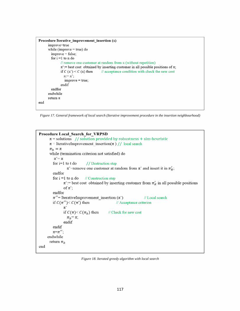
117

Figure 17. General framework of local search (Iterative improvement procedure in the insertion neighbourhood)

Figure 18. Iterated greedy algorithm with local search

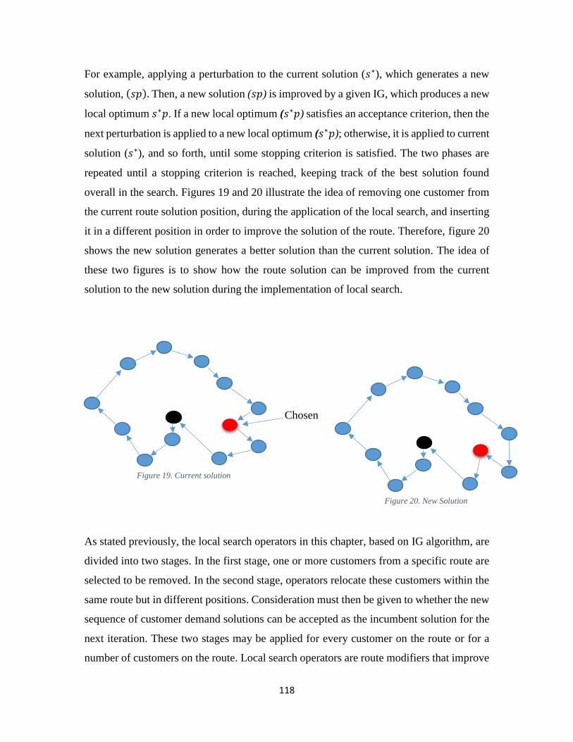
118

For example, applying a perturbation to the current solution (𝑠∗), which generates a new

solution, (𝑠𝑝). Then, a new solution (𝑠𝑝) is improved by a given IG, which produces a new

local optimum 𝑠∗𝑝. If a new local optimum (𝑠∗𝑝) satisfies an acceptance criterion, then the

next perturbation is applied to a new local optimum (𝑠∗𝑝); otherwise, it is applied to current

solution (𝑠∗), and so forth, until some stopping criterion is satisfied. The two phases are

repeated until a stopping criterion is reached, keeping track of the best solution found

overall in the search. Figures 19 and 20 illustrate the idea of removing one customer from

the current route solution position, during the application of the local search, and inserting

it in a different position in order to improve the solution of the route. Therefore, figure 20

shows the new solution generates a better solution than the current solution. The idea of

these two figures is to show how the route solution can be improved from the current

solution to the new solution during the implementation of local search.

As stated previously, the local search operators in this chapter, based on IG algorithm, are

divided into two stages. In the first stage, one or more customers from a specific route are

selected to be removed. In the second stage, operators relocate these customers within the

same route but in different positions. Consideration must then be given to whether the new

sequence of customer demand solutions can be accepted as the incumbent solution for the

next iteration. These two stages may be applied for every customer on the route or for a

number of customers on the route. Local search operators are route modifiers that improve

Chosen

Figure 19. Current solution

Figure 20. New Solution

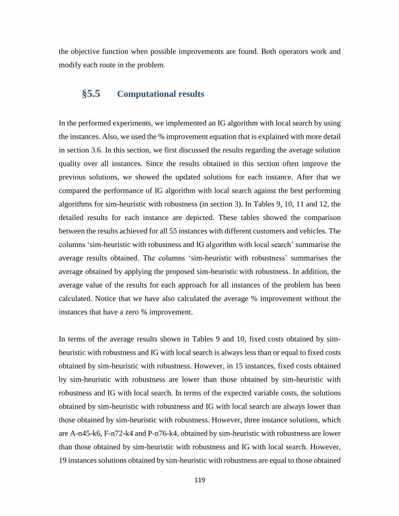
119

the objective function when possible improvements are found. Both operators work and

modify each route in the problem.

§5.5 Computational results

In the performed experiments, we implemented an IG algorithm with local search by using

the instances. Also, we used the % improvement equation that is explained with more detail

in section 3.6. In this section, we first discussed the results regarding the average solution

quality over all instances. Since the results obtained in this section often improve the

previous solutions, we showed the updated solutions for each instance. After that we

compared the performance of IG algorithm with local search against the best performing

algorithms for sim-heuristic with robustness (in section 3). In Tables 9, 10, 11 and 12, the

detailed results for each instance are depicted. These tables showed the comparison

between the results achieved for all 55 instances with different customers and vehicles. The

columns ‘sim-heuristic with robustness and IG algorithm with local search’ summarise the

average results obtained. The columns ‘sim-heuristic with robustness’ summarises the

average obtained by applying the proposed sim-heuristic with robustness. In addition, the

average value of the results for each approach for all instances of the problem has been

calculated. Notice that we have also calculated the average % improvement without the

instances that have a zero % improvement.

In terms of the average results shown in Tables 9 and 10, fixed costs obtained by sim-

heuristic with robustness and IG with local search is always less than or equal to fixed costs

obtained by sim-heuristic with robustness. However, in 15 instances, fixed costs obtained

by sim-heuristic with robustness are lower than those obtained by sim-heuristic with

robustness and IG with local search. In terms of the expected variable costs, the solutions

obtained by sim-heuristic with robustness and IG with local search are always lower than

those obtained by sim-heuristic with robustness. However, three instance solutions, which

are A-n45-k6, F-n72-k4 and P-n76-k4, obtained by sim-heuristic with robustness are lower

than those obtained by sim-heuristic with robustness and IG with local search. However,

19 instances solutions obtained by sim-heuristic with robustness are equal to those obtained

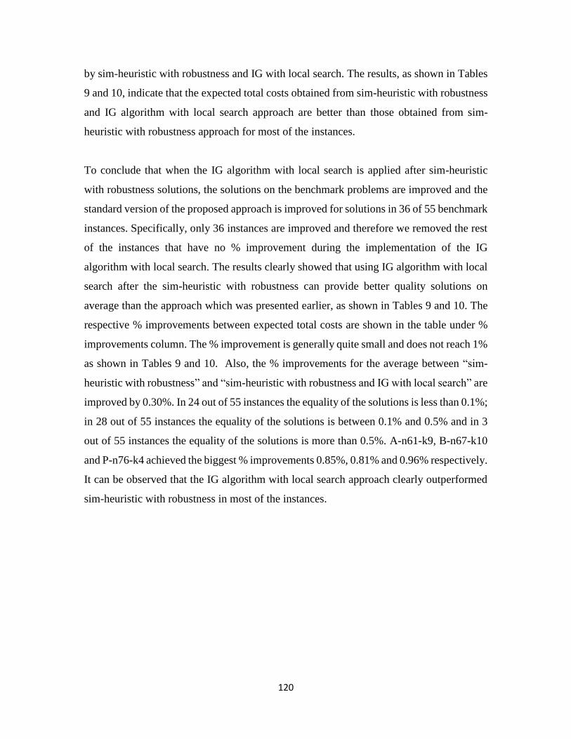
120

by sim-heuristic with robustness and IG with local search. The results, as shown in Tables

9 and 10, indicate that the expected total costs obtained from sim-heuristic with robustness

and IG algorithm with local search approach are better than those obtained from sim-

heuristic with robustness approach for most of the instances.

To conclude that when the IG algorithm with local search is applied after sim-heuristic

with robustness solutions, the solutions on the benchmark problems are improved and the

standard version of the proposed approach is improved for solutions in 36 of 55 benchmark

instances. Specifically, only 36 instances are improved and therefore we removed the rest

of the instances that have no % improvement during the implementation of the IG

algorithm with local search. The results clearly showed that using IG algorithm with local

search after the sim-heuristic with robustness can provide better quality solutions on

average than the approach which was presented earlier, as shown in Tables 9 and 10. The

respective % improvements between expected total costs are shown in the table under %

improvements column. The % improvement is generally quite small and does not reach 1%

as shown in Tables 9 and 10. Also, the % improvements for the average between “sim-

heuristic with robustness” and “sim-heuristic with robustness and IG with local search” are

improved by 0.30%. In 24 out of 55 instances the equality of the solutions is less than 0.1%;

in 28 out of 55 instances the equality of the solutions is between 0.1% and 0.5% and in 3

out of 55 instances the equality of the solutions is more than 0.5%. A-n61-k9, B-n67-k10

and P-n76-k4 achieved the biggest % improvements 0.85%, 0.81% and 0.96% respectively.

It can be observed that the IG algorithm with local search approach clearly outperformed

sim-heuristic with robustness in most of the instances.

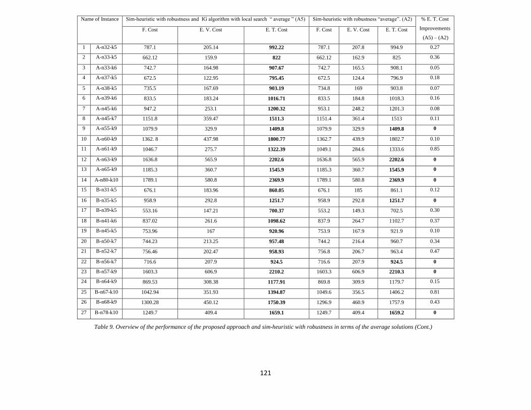
121

Name of Instance Sim-heuristic with robustness and IG algorithm with local search “ average ” (A5) Sim-heuristic with robustness “average”. (A2) % E. T. Cost

Improvements

(A5) – (A2)

F. Cost E. V. Cost E. T. Cost F. Cost E. V. Cost E. T. Cost

1 A-n32-k5 787.1 205.14 992.22 787.1 207.8 994.9 0.27

2 A-n33-k5 662.12 159.9 822 662.12 162.9 825 0.36

3 A-n33-k6 742.7 164.98 907.67 742.7 165.5 908.1 0.05

4 A-n37-k5 672.5 122.95 795.45 672.5 124.4 796.9 0.18

5 A-n38-k5 735.5 167.69 903.19 734.8 169 903.8 0.07

6 A-n39-k6 833.5 183.24 1016.71 833.5 184.8 1018.3 0.16

7 A-n45-k6 947.2 253.1 1200.32 953.1 248.2 1201.3 0.08

8 A-n45-k7 1151.8 359.47 1511.3 1151.4 361.4 1513 0.11

9 A-n55-k9 1079.9 329.9 1409.8 1079.9 329.9 1409.8 0

10 A-n60-k9 1362. 8 437.98 1800.77 1362.7 439.9 1802.7 0.10

11 A-n61-k9 1046.7 275.7 1322.39 1049.1 284.6 1333.6 0.85

12 A-n63-k9 1636.8 565.9 2202.6 1636.8 565.9 2202.6 0

13 A-n65-k9 1185.3 360.7 1545.9 1185.3 360.7 1545.9 0

14 A-n80-k10 1789.1 580.8 2369.9 1789.1 580.8 2369.9 0

15 B-n31-k5 676.1 183.96 860.05 676.1 185 861.1 0.12

16 B-n35-k5 958.9 292.8 1251.7 958.9 292.8 1251.7 0

17 B-n39-k5 553.16 147.21 700.37 553.2 149.3 702.5 0.30

18 B-n41-k6 837.02 261.6 1098.62 837.9 264.7 1102.7 0.37

19 B-n45-k5 753.96 167 920.96 753.9 167.9 921.9 0.10

20 B-n50-k7 744.23 213.25 957.48 744.2 216.4 960.7 0.34

21 B-n52-k7 756.46 202.47 958.93 756.8 206.7 963.4 0.47

22 B-n56-k7 716.6 207.9 924.5 716.6 207.9 924.5 0

23 B-n57-k9 1603.3 606.9 2210.2 1603.3 606.9 2210.3 0

24 B-n64-k9 869.53 308.38 1177.91 869.8 309.9 1179.7 0.15

25 B-n67-k10 1042.94 351.93 1394.87 1049.6 356.5 1406.2 0.81

26 B-n68-k9 1300.28 450.12 1750.39 1296.9 460.9 1757.9 0.43

27 B-n78-k10 1249.7 409.4 1659.1 1249.7 409.4 1659.2 0

Table 9. Overview of the performance of the proposed approach and sim-heuristic with robustness in terms of the average solutions (Cont.)

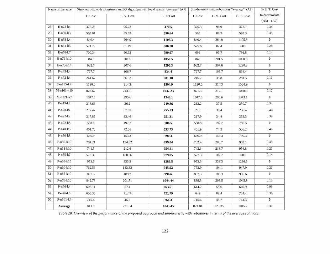
122

Name of Instance Sim-heuristic with robustness and IG algorithm with local search “average” (A5) Sim-heuristic with robustness “average”. (A2) % E. T. Cost

Improvements

(A5) – (A2)

F. Cost E. V. Cost E. T. Cost F. Cost E. V. Cost E. T. Cost

28 E-n22-k4 375.28 95.22 470.5 375.3 96.9 472.1 0.34

29 E-n30-k3 505.01 85.63 590.64 505 88.3 593.3 0.45

30 E-n33-k4 840.4 264.9 1105.3 840.4 264.9 1105.3 0

31 E-n51-k5 524.79 81.49 606.28 525.6 82.4 608 0.28

32 E-n76-k7 700.34 90.33 790.67 698 93.7 791.8 0.14

33 E-n76-k10 849 201.5 1050.5 849 201.5 1050.5 0

34 E-n76-k14 982.7 307.6 1290.3 982.7 307.6 1290.3 0

35 F-n45-k4 727.7 106.7 834.4 727.7 106.7 834.4 0

36 F-n72-k4 244.67 36.52 281.18 245.7 35.8 281.5 0.11

37 F-n135-k7 1190.6 314.3 1504.9 1190.6 314.3 1504.9 0

38 M-n101-k10 823.62 213.61 1037.23 821.5 217.1 1038.5 0.12

39 M-n121-k7 1047.5 295.6 1343.1 1047.5 295.6 1343.1 0

40 P-n19-k2 213.66 36.2 249.86 213.2 37.5 250.7 0.34

41 P-n20-k2 217.42 37.81 255.23 218 38.4 256.4 0.46

42 P-n22-k2 217.85 33.46 251.31 217.9 34.4 252.3 0.39

43 P-n22-k8 588.8 197.7 786.5 588.8 197.7 786.5 0

44 P-n40-k5 461.73 72.01 533.73 461.9 74.2 536.2 0.46

45 P-n50-k8 636.9 153.3 790.3 636.9 153.3 790.3 0

46 P-n50-k10 704.21 194.82 899.04 702.4 200.7 903.1 0.45

47 P-n51-k10 741.5 212.6 954.41 743.1 213.7 956.8 0.25

48 P-n55-k7 578.39 100.66 679.05 577.3 102.7 680 0.14

49 P-n55-k15 953.3 333.3 1286.5 953.3 333.3 1286.5 0

50 P-n60-k10 762.59 183.33 945.92 753.9 194.1 947.9 0.21

51 P-n65-k10 807.3 189.3 996.6 807.3 189.3 996.6 0

52 P-n70-k10 842.73 201.71 1044.44 839.3 206.5 1045.8 0.13

53 P-n76-k4 606.11 57.4 663.51 614.2 55.6 669.9 0.96

54 P-n76-k5 650.36 71.43 721.79 642 82.4 724.4 0.36

55 P-n101-k4 715.6 45.7 761.3 715.6 45.7 761.3 0

Average 811.9 221.54 1043.45 821.84 223.35 1045.2 0.30

Table 10. Overview of the performance of the proposed approach and sim-heuristic with robustness in terms of the average solutions

123

Tables 11 and 12 showed a list of best results that are obtained in this experiment for the

VRPSD. Columns 3 to 5 represented the solution obtained by the methodology that is

proposed in this chapter when a 100% of the vehicle maximum capacity is considered.

Also, these columns showed respectively the fixed cost, expected variable cost and

expected total cost found by the methodology that is proposed in this chapter. The IG

algorithm with local search is able to improve solutions for most of the VRPSD instances.

On the other hand, columns 6 - 8 showed the results obtained by sim-heuristic and

robustness. In addition, in this section, we presented an extensive experimental comparison

of the proposed robust model with sim-heuristic and IG algorithm with local search

solutions and compared the performance to sim-heuristic with robustness solutions.

Therefore, we compared the best solution costs found by our approaches in Tables 11 and

12. These tables showed the results obtained in this experiment and we reported the cost

of the best solution found in any run of the heuristic.

In terms of the best results as shown in Tables 11 and 12, fixed costs obtained by sim-

heuristic with robustness and IG with local search are always lower or equal to those

obtained by sim-heuristic with robustness. However, in 8 instances, fixed costs obtained

by sim-heuristic with robustness are lower than those obtained by sim-heuristic with

robustness and IG with local search. Variable expected costs obtained by sim-heuristic with

robustness and IG with local search are always lower than those obtained by sim heuristic

with robustness. However, in 3 instances which are F-n72-k4, P-n70-k10 and P-n76-k5,

expected variable costs obtained by sim-heuristic with robustness are lower than those

obtained by sim-heuristic with robustness and IG with local search. The results, as shown

in Tables 11 and 12, indicate that the expected total cost obtained from sim-heuristic with

robustness and IG algorithm with local search approach are better than those obtained from

sim-heuristic with robustness for 36 out of 55 instances.

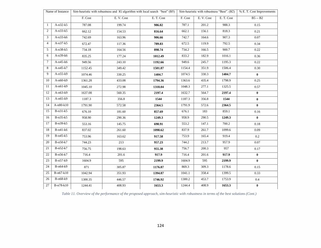
124

Name of Instance Sim-heuristic with robustness and IG algorithm with local search “best” (B5) Sim-heuristic with robustness “Best”. (B2) % E. T. Cost Improvements

F. Cost E. V. Cost E. T. Cost F. Cost E. V. Cost E. T. Cost B5 -- B2

1 A-n32-k5 787.08 199.74 986.82 787.1 201.2 988.3 0.15

2 A-n33-k5 662.12 154.53 816.64 662.1 156.1 818.3 0.21

3 A-n33-k6 742.69 163.96 906.66 742.7 164.6 907.3 0.07

4 A-n37-k5 672.47 117.36 789.83 672.5 119.9 792.5 0.34

5 A-n38-k5 734.18 164.56 898.74 734.2 166.5 900.7 0.22

6 A-n39-k6 835.25 177.24 1012.49 833.2 182.9 1016.1 0.36

7 A-n45-k6 949.56 243.10 1192.66 949.6 245.7 1195.3 0.22

8 A-n45-k7 1152.45 349.42 1501.87 1154.4 351.9 1506.4 0.30

9 A-n55-k9 1074.46 330.25 1404.7 1074.5 330.3 1404.7 0

10 A-n60-k9 1361.28 433.08 1794.36 1363.6 435.4 1798.9 0.25

11 A-n61-k9 1045.10 272.98 1318.04 1048.3 277.1 1325.5 0.57

12 A-n63-k9 1637.08 560.35 2197.4 1632.7 564.7 2197.4 0

13 A-n65-k9 1187.3 356.8 1544 1187.3 356.8 1544 0

14 A-n80-k10 1791.90 572.58 2364.5 1791.9 572.6 2364.5 0

15 B-n31-k5 676.10 181.60 857.69 676.1 183 859.1 0.16

16 B-n35-k5 958.90 290.36 1249.3 958.9 290.5 1249.3 0

17 B-n39-k5 553.16 145.75 698.91 553.2 147.1 700.2 0.18

18 B-n41-k6 837.02 261.60 1098.62 837.9 261.7 1099.6 0.09

19 B-n45-k5 753.96 163.62 917.58 753.9 165.4 919.4 0.2

20 B-n50-k7 744.23 213 957.23 744.2 213.7 957.9 0.07

21 B-n52-k7 756.75 198.63 955.38 756.7 200.3 957 0.17

22 B-n56-k7 716.4 201.6 917.9 716.4 201.6 917.9 0

23 B-n57-k9 1604.9 595 2199.9 1604.9 595 2199.9 0

24 B-n64-k9 871 305.87 1176.87 869.3 309.3 1178.6 0.15

25 B-n67-k10 1042.94 351.93 1394.87 1041.1 358.4 1399.5 0.33

26 B-n68-k9 1300.35 446.57 1746.92 1300.2 453.7 1753.9 0.4

27 B-n78-k10 1244.41 408.93 1653.3 1244.4 408.9 1653.3 0

Table 11. Overview of the performance of the proposed approach, sim-heuristic with robustness in terms of the best solutions (Cont.)

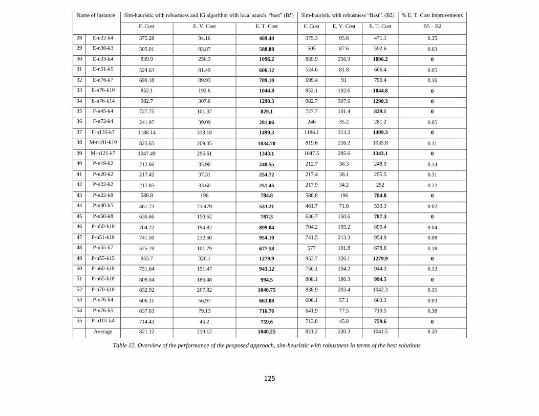
125

Name of Instance Sim-heuristic with robustness and IG algorithm with local search “best” (B5) Sim-heuristic with robustness “Best”. (B2) % E. T. Cost Improvements

F. Cost E. V. Cost E. T. Cost F. Cost E. V. Cost E. T. Cost B5 – B2

28 E-n22-k4 375.28 94.16 469.44 375.3 95.8 471.1 0.35

29 E-n30-k3 505.01 83.87 588.88 505 87.6 592.6 0.63

30 E-n33-k4 839.9 256.3 1096.2 839.9 256.3 1096.2 0

31 E-n51-k5 524.63 81.49 606.12 524.6 81.8 606.4 0.05

32 E-n76-k7 699.18 89.93 789.10 699.4 91 790.4 0.16

33 E-n76-k10 852.1 192.6 1044.8 852.1 192.6 1044.8 0

34 E-n76-k14 982.7 307.6 1290.3 982.7 307.6 1290.3 0

35 F-n45-k4 727.75 101.37 829.1 727.7 101.4 829.1 0

36 F-n72-k4 241.97 39.09 281.06 246 35.2 281.2 0.05

37 F-n135-k7 1186.14 313.18 1499.3 1186.1 313.2 1499.3 0

38 M-n101-k10 825.65 209.05 1034.70 819.6 216.2 1035.8 0.11

39 M-n121-k7 1047.49 295.61 1343.1 1047.5 295.6 1343.1 0

40 P-n19-k2 212.66 35.90 248.55 212.7 36.3 248.9 0.14

41 P-n20-k2 217.42 37.31 254.72 217.4 38.1 255.5 0.31

42 P-n22-k2 217.85 33.60 251.45 217.9 34.2 252 0.22

43 P-n22-k8 588.8 196 784.8 588.8 196 784.8 0

44 P-n40-k5 461.73 71.479 533.21 461.7 71.6 533.3 0.02

45 P-n50-k8 636.66 150.62 787.3 636.7 150.6 787.3 0

46 P-n50-k10 704.22 194.82 899.04 704.2 195.2 899.4 0.04

47 P-n51-k10 741.50 212.60 954.10 741.5 213.3 954.9 0.08

48 P-n55-k7 575.79 101.79 677.58 577 101.8 678.8 0.18

49 P-n55-k15 953.7 326.1 1279.9 953.7 326.1 1279.9 0

50 P-n60-k10 751.64 191.47 943.12 750.1 194.2 944.3 0.13

51 P-n65-k10 808.04 186.48 994.5 808.1 186.3 994.5 0

52 P-n70-k10 832.92 207.82 1040.75 838.9 203.4 1042.3 0.15

53 P-n76-k4 606.11 56.97 663.08 606.1 57.1 663.3 0.03

54 P-n76-k5 637.63 79.13 716.76 641.9 77.5 719.5 0.38

55 P-n101-k4 714.43 45.2 759.6 713.8 45.8 759.6 0

Average 821.12 219.12 1040.25 821.2 220.3 1041.5 0.20

Table 12. Overview of the performance of the proposed approach, sim-heuristic with robustness in terms of the best solutions

126

It should be noticed that the experiments represented in this table illustrate that the fixed cost

could be higher but the expected cost variable would be lower, and so this could lead to lower

than expected total costs ultimately, which could be further minimised. Despite the limited

repetition for each instance, the approach is able to improve solutions for the VRPSD (average

% improvement of 0.20% with respect to the known solutions). Notice that we have calculated

the average of % improvement without the instances that have a zero % improvement. This

result allowed to validate the algorithm employed to improve solutions. In addition, the bottom

row in the Tables show the average value of the results for each approach for all instances of

the problems, and the comparison between these approaches.

The last column presented the % improvement between these two approaches, which are “sim-

heuristic with robustness” and “sim-heuristic with robustness and IG algorithm with local

search”. Furthermore, each row in the tables corresponded to one instance of a problem and its

detail. The comparison of these best expected total costs are shown in Tables 11 and 12. The

expected total costs for each approach has been presented in the tables. The solutions given by

the approach put forward in this study are on average better than other solutions given,

achieving 1040.25 for the average expected total cost for all instances.

The % improvement is generally quite small and does not reach 1% when sim-heuristic with

robustness are compared to sim-heuristic with robustness and IG algorithm with local search.

The solution value obtained by the approach put forward in this study improved the expected

total cost solution. Therefore, the results clearly showed that using IG algorithm with local

search after the method in those instances, can provide better quality solutions than other

methods. As it can be seen, the proposed algorithm achieved better results than sim-heuristic

with robustness. Also, the % improvement in the quality of the solutions to these approach

instances is between 0% and 0.63%. In 28 out of 55 instances the equality of the solutions is

less than 0.1%, in 19 out of 55 instances the equality of the solutions is between 0.1% to 0.3%

and in 8 out of 55 instances the equality of the solutions is more than 0.3%. Therefore, using

IG algorithm with local search is the most efficient method in order to solve the VRPSD. In

addition, the most interesting result is that E-n30-k3 achieved the biggest % improvement

between the approach presented in this chapter and sim-heuristic with robustness approach

which is improved by 0.63% and the solutions obtained by using 3 routes. The smallest %

improvement which is zero has been omitted from the calculation of the average in the last

row. Furthermore, as shown in Tables 11 and 12, using the IG algorithm with local search is

127

effective in solving all VRPSD instances. It has the ability to improve upon the best known

solutions and improved 36 out of 55 instances, which means that 19 out of 55 showed no %

improvement. It can be seen that expected total costs obtained by sim-heuristic with robustness

and IG algorithm with local search has smaller optimality % improvements than expected total

costs obtained by sim-heuristic with robustness, for most instances, and the average between

these approaches is 0.20 %. Notice that sim-heuristic with robustness and IG algorithm with

local search can be improved upon and a solution that is at least as good as the previously best

known solutions can be found.

The findings of computational experiments indicated that sim-heuristic with robustness and IG

algorithm with a local search has been shown to be an effective technique with the approach

proposed earlier in the thesis, in terms of improving the solution quality of the VRPSD

instances. One typically defines sim-heuristic with robustness and IG algorithm with a local

search that consists of feasible solutions that can be achieved from an existing solution, through

well-defined operations such as reinserting a customer to a new position in the same route. It

should be noticed that when we consider small numbers of repetition, fewer and better solutions

are likely to be achieved. However, when we consider larger number of repetition, more

feasible solutions have to be examined at each iteration and better solutions can be achieved,

but the algorithm eventually gets slower.

§5.6 Conclusion

This chapter dealt with the VRPSD by using IG algorithm with local search and sim-heuristic

with robustness. The combination of the above mentioned method seems to have played an

essential role in developing a better routing to minimise the transportation costs in VRPSD.

The IG algorithm with local search adapts the best solution found by changing it to give a better

cost solution. That is, the solution cost is exchanged with the first solution cost that improves

the cost. On the other hand, if there is no solution cost improvement to the current solution, the

current solution cost is considered to be the local optimal solution cost. The search procedure

is repeated until a pre-specified stopping condition is satisfied. The researchers used the IG

algorithm with local search after applying sim-heuristic with robustness to obtain high quality

solutions especially for the VRPSD. It was also proven that, by using well-known benchmark

instances, the implementation of these approaches enhanced solutions. Moreover, based on

128

some properties, IG algorithm with a local search algorithm can improve the heuristic to get

high-quality solutions for the VRPSD. From the experiment solutions, one could conclude that

the approach that is presented in this chapter is able to improve VRPSD solutions to within

65.45% of used instances. Thus, 34.5% would show no improvements.

The following observations have been made following the evaluation of the results:

It is clearly better to use the CWS steps to compute the initial solutions to the problems.

The solution quality generated by using IG algorithm with the local search algorithms

can be arbitrarily good if an arbitrarily large number of repetitions are permitted.

Suitable choices in terms of the number of repetitions depend on the execution and copy

time of the problem. If they are large, a large number of repetitions should be used,

since the resulting improvement to the problem dominates the increased running time

of the algorithms. Conversely, if the running times are small, a small number of

repetitions should be used.

129

Chapter 6 : NADEC case study: VRPSD for

distribution of food in a real urban context.

§6.1 Introduction

The distribution of food products has received a great deal of attention lately from companies

and researchers all over the world. There are different aims of the researchers, e.g., minimising

the total transportation costs, reducing logistics and distribution costs, promoting food safety

and others. Hence, effective and efficient management of food product transportation and

distribution is becoming increasingly important with respect to both logistics and

marketing/sales for order delivery times. It is important for decision makers to make a good

plan in order to deliver the demands of the customers. If there are any problems, it significantly

affects the delivery costs and the profit.

In this chapter, the work studied a real-life problem faced by a Saudi food distribution company

that supplies a wide range of food solutions for different range of customers. A food solution

is defined as a service that provides a quick response to customer orders for a set of food

products. The vision of The National Agricultural Development Company (NADEC) is to be

one of the best operating in the business sector in terms of quality and achieving high

operational efficiency. NADEC Company are considered one of the biggest Food and

Agricultural Company’s in both the Middle East and North Africa. NADEC established in 1981

by royal decree is a joint stock public company. Therefore, 20% of the company is owned by

the government and the rest publicly traded on the Saudi Stock Exchange, which is around

80%. In addition, NADEC is considered to be one of the largest integrated dairy company’ in

the world. NADEC Company attempts to provide better, tastiest, nicest and healthiest

nutritional products. The main NADEC office is located in Riyadh. Figure 21 represents the

map of the Kingdom of Saudi Arabia and of the NADEC Company. More details about

NADEC Company are available at http://www.nadec.com.sa/en-us/home.aspx . This link has

more details and contains reports for the company with products and other details such as terms

of financial performance for different years. This chapter is organised as follows: A brief

literature review is presented in section 6.2. In section 6.3, we provided a brief explanation and

review of NADEC Company. Section 6.4 gave details about the Company products. Section

6.5 gave a detailed description of NADEC instance. Numerical results are presented in section

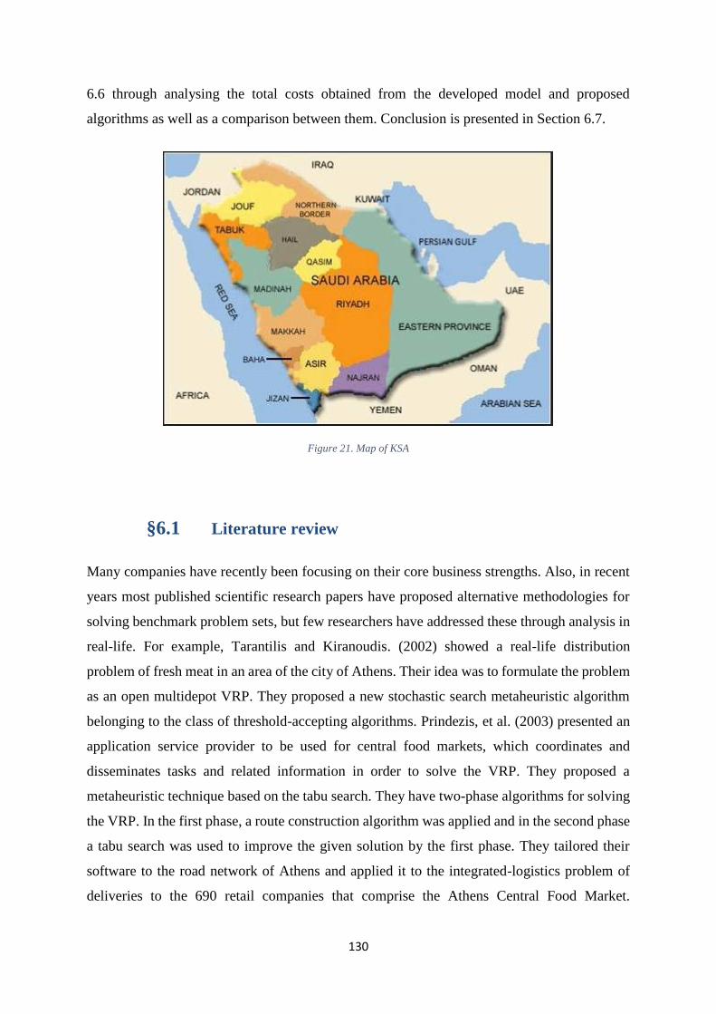
130

6.6 through analysing the total costs obtained from the developed model and proposed

algorithms as well as a comparison between them. Conclusion is presented in Section 6.7.

Figure 21. Map of KSA

§6.1 Literature review

Many companies have recently been focusing on their core business strengths. Also, in recent

years most published scientific research papers have proposed alternative methodologies for

solving benchmark problem sets, but few researchers have addressed these through analysis in

real-life. For example, Tarantilis and Kiranoudis. (2002) showed a real-life distribution

problem of fresh meat in an area of the city of Athens. Their idea was to formulate the problem

as an open multidepot VRP. They proposed a new stochastic search metaheuristic algorithm

belonging to the class of threshold-accepting algorithms. Prindezis, et al. (2003) presented an

application service provider to be used for central food markets, which coordinates and

disseminates tasks and related information in order to solve the VRP. They proposed a

metaheuristic technique based on the tabu search. They have two-phase algorithms for solving

the VRP. In the first phase, a route construction algorithm was applied and in the second phase

a tabu search was used to improve the given solution by the first phase. They tailored their

software to the road network of Athens and applied it to the integrated-logistics problem of

deliveries to the 690 retail companies that comprise the Athens Central Food Market.

131

Amponsah and Salhi. (2004) proposed an efficient heuristic for the routing problem of the

collection of garbage in developing countries. Their idea was to formulate the problem as a

Capacitated Arc Routing Problem (CARP) and minimise the environmental effect due to the

smell of the garbage and total collection cost in a bi-objective model. They used a look-ahead

strategy; this strategy gives the possibility to choose from a pool of solutions, the one which

best solves the problem. Osvald and Stirn (2008) formulated the problem as a Vehicle Routing

Problem with Time Windows and Time-Dependent travel-times (VRPTWTD). The time that

the food spends on the vehicles is the most important factor. The model considers the impact

of the perishability as part of the overall distribution costs and a heuristic approach. Also, they

proposed tabu search to solve the problem.

Amorim et al. (2012) showed one of a successful application of operations research techniques

in guiding the decision making process to achieve a superior operational efficiency in core

activities. This kind of problem can be described as a heterogeneous fleet site dependent vehicle

routing problem, with multiple time windows faced by a Portuguese food distribution company

on a daily basis. They proposed the adaptive large neighbourhood search method, which was

proven to be effective to solve a number of different vehicle routing problems. The idea behind

their study was to compare the solution against those of the company and the impact that the

proposed decision support tool may have in terms of cost savings is shown. The algorithm

converges quickly giving the planner considerably more time to focus on value-added tasks,

rather than manually correct the routing schedule. The main objective of (Li et al., 2015) was

to achieve the optimal distribution routes for fresh fruits and vegetables, considering different

road classes with the least amount of logistics costs. They proposed an improved genetic

algorithm in order to solve the problem. A fruit delivery route among the 13 cities in Jiangsu

Province was used as a real analysis case. In terms of the computational results of the real case,

the simulation results showed that the vehicle routing problem with time windows are able to

significantly influence total delivery costs compared with traditional VRP models. The aim of

the comparison between four models is to predict the total cost and actual total cost in

distribution. Also this comparison showed that the improved genetic algorithm is superior to

other methods that used.

Mungwattana, et al. (2016) presented a practical case study of a heterogeneous fleet vehicle

routing problem with different constraints that mainly provides services to a big industrial

estate in Thailand. Decision making problems related to distribution management are classified

132

into three levels (1) Strategic level for decision-making relates to the location of facilities (e.g.

central depots). In this level, the decision is very important because the locations of the facilities

have many effects on the transportation costs of different operations in lower levels. (2) Tactical

level relates to the problem of the size of the fleet and mix determination. In this level, the decision

will be made based on the given demand and facilities. (3) Operational level relates to the problem

of routing and scheduling of the existing vehicles and staffing of such vehicles. In this level, this

decision should be made on day-to-day basis.

§6.1 NADEC Company

6.1.1 NADEC foods

NADEC put the family’s health as a high priority, which is committed to the highest standards

of quality and continuous development to meet the growing requirements of customers. It

provides more than 100 products including fresh milk, Laban, a variety of yoghurt and cheese,

and a wide range of fruit juices to suit different occasions as well as to meet the needs of all

customers. Nowadays, NADEC becomes one of the leading foods and juices companies in the

region. NADEC has six farms including approximately 60,000 cows as well as two

manufacturers producing more than 1.5 million litres of milk per day. Furthermore, NADEC

laboratories are equipped with the latest advanced technology and administered by a team of

experts in the field of nutrition and quality. Also, the experts apply strict procedure during the

stages of production to ensure that they meet the highest quality standards. NADEC is

committed to recruiting the best people and also keen to train and develop their skills and

provide them with the latest technology.

Agricultural production is one of the most significant activities in the company and integrates

with the objectives of the Kingdom of Saudi Arabia (KSA) in promoting food self-sufficiency

and reduce dependence on imports. The agricultural section provides a variety of different

products such as onions, olives, corn, potatoes and fruits. Also, other food such as nutritional

animal fodder which is used to feed the cows in the farms. Here are some examples about the

products: (1) fruits such as plums, apricots and peaches, (2) vegetables such as onions, tomatoes

and potatoes, (3) agricultural crops such as, herb Rhodes and corn are grown on various

locations in the KSA: Haradh, Wadi Al-Dawasser, Hail and Al-Jouf. There are some points

that made NADEC one of the best companys such as it uses the latest technology to ensure the

133

best quality of food products and agricultural crops including the use of advanced systems such

as the DACOM system to rationalise the irrigation of water. This system measures the rate of

humidity and temperature in the soil and uses sophisticated measurement techniques to monitor

and control the amount of water released to the plants to reduce the amount of water wasted.

As a result of the implementation of best agricultural practices from around the world, NADEC

has achieved many successes and got several international certificates for farming and quality

of both their products and crops. NADEC aims through economic development projects to

reduce imports and increase reliance on the national economy, and promote participation in the

agricultural sector for the Kingdom’s future sustainability.

6.1.2 NADEC agricultural projects in the KSA

NADEC is successful due to several factors which include, staff efficiency, production

procedures and the technology used. NADEC’s history also includes some of the key projects

that have helped to support the vision and objectives of both the government and the Board of

Directors. Figure 22 shows the geographical location of all the projects in the KSA. It should

notice that these projects are located in different positions in KSA and that each one of the

projects can produce different products. The first project is Haradh project which is located

250km southeast of Riyadh, and is one of the most important sites that has an area of 37,500

hectares. It contains several things such as dairy factories and cattle farms. In addition, there

are protected homes which cover an estimated area of 12.5 hectares. Also, the project has a

number of palm trees. The second project is Wadi Al-Dawasser project which is located 650km

southwest of Riyadh. This project covers an area of 40,000 hectares. This project is specialised

cultivation of agricultural crops, for example, vegetables including potatoes, onions and

tomatoes and others such as wheat, corn, and fodder. The third project is Hail project which is

located 580 km southwest of Riyadh, and is a significant project; it is fully grown in terms of

producing wheat and fodder and corn. In addition, there is one of the largest seed treatment

plants in the KSA located in this project. The final project is Al Jouf project which is located

around 1,250km north of Riyadh. The main advantage of the Al Jouf project location is that it

offers a suitable climate for the cultivation of many varieties of fruit trees for example, apricots,

peaches and plums. It also produces olive oil.

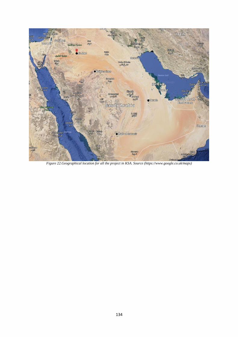
134

Figure 22.Geographical location for all the project in KSA. Source (https://www.google.co.uk/maps)

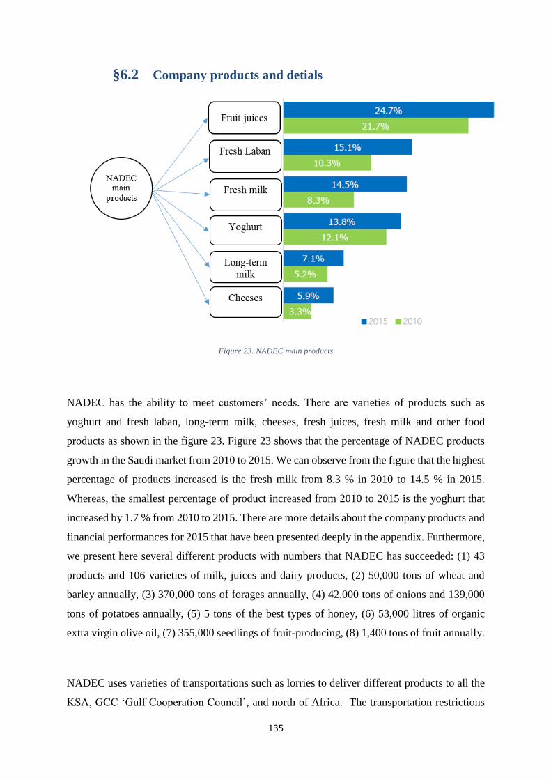
135

§6.2 Company products and detials

Figure 23. NADEC main products

NADEC has the ability to meet customers’ needs. There are varieties of products such as

yoghurt and fresh laban, long-term milk, cheeses, fresh juices, fresh milk and other food

products as shown in the figure 23. Figure 23 shows that the percentage of NADEC products

growth in the Saudi market from 2010 to 2015. We can observe from the figure that the highest

percentage of products increased is the fresh milk from 8.3 % in 2010 to 14.5 % in 2015.

Whereas, the smallest percentage of product increased from 2010 to 2015 is the yoghurt that

increased by 1.7 % from 2010 to 2015. There are more details about the company products and

financial performances for 2015 that have been presented deeply in the appendix. Furthermore,

we present here several different products with numbers that NADEC has succeeded: (1) 43

products and 106 varieties of milk, juices and dairy products, (2) 50,000 tons of wheat and

barley annually, (3) 370,000 tons of forages annually, (4) 42,000 tons of onions and 139,000

tons of potatoes annually, (5) 5 tons of the best types of honey, (6) 53,000 litres of organic

extra virgin olive oil, (7) 355,000 seedlings of fruit-producing, (8) 1,400 tons of fruit annually.

NADEC uses varieties of transportations such as lorries to deliver different products to all the

KSA, GCC ‘Gulf Cooperation Council’, and north of Africa. The transportation restrictions

136

are defined inside the city. Also, the orientation of streets, traffic lights and road repairs can

influence the daily routing planning. NADEC follows various standards to divide the cities.

For example the city of Riyadh, NADEC divides into five geographic regions which are north,

south, east, west, and the middle of Riyadh. NADEC secures around 3500 refrigerators; also

NADEC uses a fleet of refrigerated delivery vehicles of all sizes - more than 600 vehicles.

§6.3 Company instances

NADEC Company has thousands of employees including drivers and dispatchers. The main

focus of the NADEC Company is considered to be the problem involving the food distribution.

It owns a fleet of vehicles such as small vehicles, big vehicles, container trucks and others.

Furthermore, the vehicles have different capacities to serve a variety of customer demands.

Vehicles have to start and end at the central depot and start roughly between 8 and 9 a.m. in

the morning with a work-day of around 7-9 hours. The company has to adhere to the

government’s regulations stipulating the rules for drivers’ working and rest hours. The daily

driving time cannot exceed 9 hours. At most 3 hours of driving is allowed before a break of 45

minutes must to be taken. The break can be split into two periods of a minimum of 15 minutes

and the second break should be at least 30 minutes. After the 45 minutes of break, the ‘clock

time’ with respect to the 3 hour limit is restarted. The regulations only consider the time spent

during the driving period and not the time spent at each stop. Additional rules exist on a weekly

and fortnightly basis. Since a vehicle’s journey consists of multiple stops of about 30-45

minutes, the driving time during a day is often between 2-4 hours. Thus, the rules considering

longer periods are rarely relevant and we will not consider these. Since the daily driving time

might be less than 3 hours, company policy dictate that a 30 minute lunch break should as a

minimum be held during the day. Thus, in brief, all vehicles start and end at the depot and the

depot start and end time is used to limit the working day. The driver rest time has been

simplified to two parts: 1) a rest break always consists of 45 minutes after a maximum of 3

hours of driving. After the break the counter is restarted, 2) a lunch break of minimum 30

minutes must be held once during the day. If a rest break is taken the lunch break is considered

as covered.

137

The NADEC Company uses an advanced program in order to record and update the data with

a small percentage of error, thus this allows the data to become more accurate. The data on the

transportation problem has been collected from the NADEC Company on the customer located

in the city of Riyadh. As the case of study, we used the information of a prepared food

distribution company located in Riyadh (KSA). The company has provided us with the delivery

address of several different customers in eight independent periods along with their demands.

On this context the number of the vehicle, the number of the customer demands, the size of the

vehicle capacity and the location of the customers itself have a remarkable influence in the

daily of route planning. The main interest of the company is to apply the developed model with

the proposed approaches to solve the routing problem. For this reason, the company must

provide information during each period (as a sample) in order to produce a preliminary result.

Therefore on a period basis, this company receives requests from these customers. So far, the

information serves as input in order to design the company’s routing planning. According to

the size of the company it is not possible to increase staff who are specialised in mathematical

software in order to apply exact methods. Therefore we prefer to have an approximated solution

algorithm embedded in a web tool, which could be used to give an automatic solution in as

little time as possible. Regarding to the future increase on demands, the company is mainly

interested in building a set of alternative routing solutions. These solutions can include a subset

of the previously specified restrictions. There is a specific constraint: each vehicle has to visit

all customers of a route with a minimum expected total cost.

NADEC’s provided us the data with delivery address of their customers as follows: eight

different periods with 32 areas in Riyadh city and also provided us the total demand of each

period of each area individually. NADEC Company has a huge fleet of different vehicles sizes

in order to deliver the demands to the customers in several different locations; the quantities

are also different. In our case, the number of vehicles will be different in each period and each

vehicle has 2000 litres capacity. So far, the company uses different types of vehicles which are

described in Table 13 with its capacity. The columns of this table shows the capacity and

quantity of available vehicles for each period ‘each period contains 13 weeks’. The aim is to

reduce the total routing costs and also execute the same deliveries with fewer routes. The main

features of the given ninth periods are summarised in Table 14 and 15. On the first column, we

presented the name of the customers which includes 32 areas. The second to the ninth column

showed the demands for each customer within different periods.

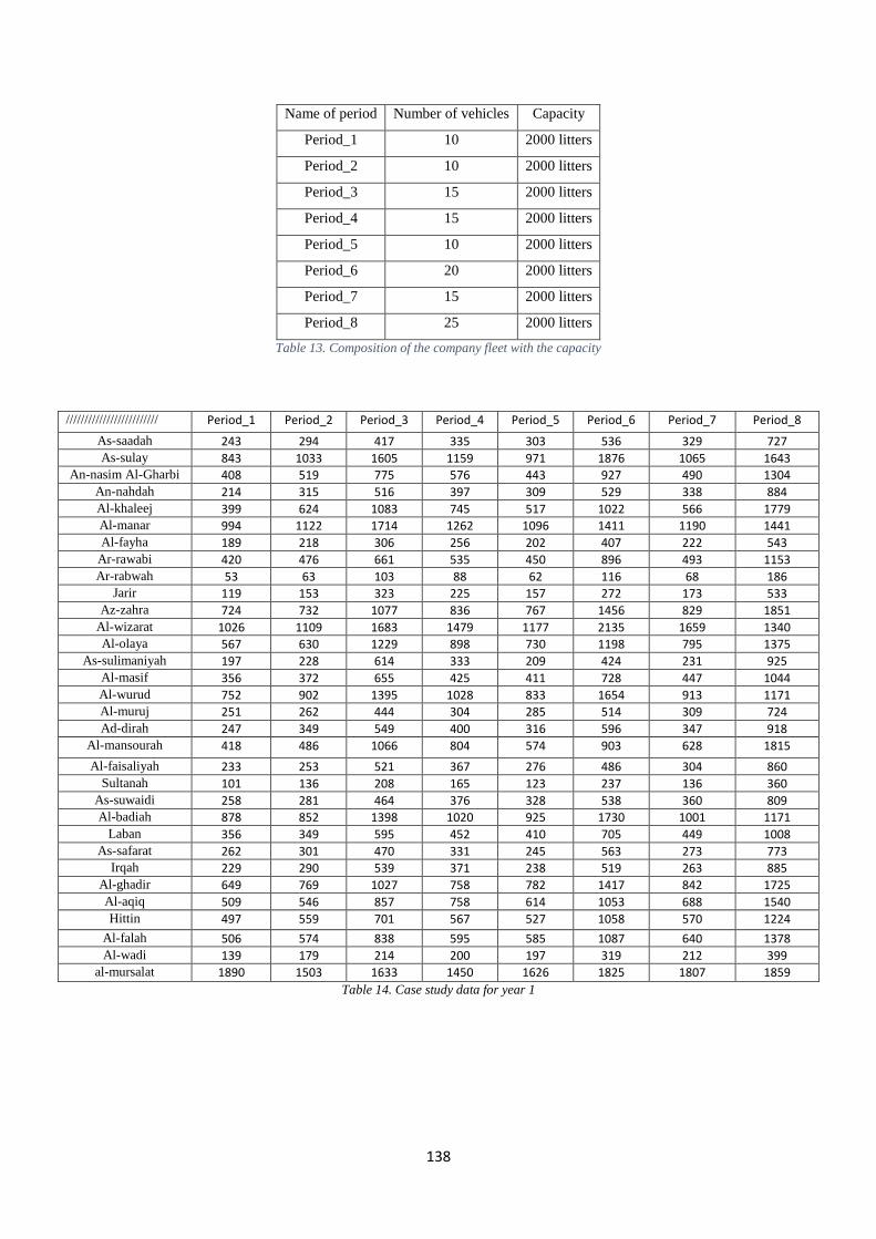
138

Name of period Number of vehicles Capacity

Period_1 10 2000 litters

Period_2 10 2000 litters

Period_3 15 2000 litters

Period_4 15 2000 litters

Period_5 10 2000 litters

Period_6 20 2000 litters

Period_7 15 2000 litters

Period_8 25 2000 litters

Table 13. Composition of the company fleet with the capacity

///////////////////////// Period_1 Period_2 Period_3 Period_4 Period_5 Period_6 Period_7 Period_8

As-saadah 243 294 417 335 303 536 329 727 As-sulay 843 1033 1605 1159 971 1876 1065 1643

An-nasim Al-Gharbi 408 519 775 576 443 927 490 1304 An-nahdah 214 315 516 397 309 529 338 884 Al-khaleej 399 624 1083 745 517 1022 566 1779 Al-manar 994 1122 1714 1262 1096 1411 1190 1441 Al-fayha 189 218 306 256 202 407 222 543

Ar-rawabi 420 476 661 535 450 896 493 1153 Ar-rabwah 53 63 103 88 62 116 68 186

Jarir 119 153 323 225 157 272 173 533 Az-zahra 724 732 1077 836 767 1456 829 1851

Al-wizarat 1026 1109 1683 1479 1177 2135 1659 1340 Al-olaya 567 630 1229 898 730 1198 795 1375

As-sulimaniyah 197 228 614 333 209 424 231 925 Al-masif 356 372 655 425 411 728 447 1044 Al-wurud 752 902 1395 1028 833 1654 913 1171 Al-muruj 251 262 444 304 285 514 309 724 Ad-dirah 247 349 549 400 316 596 347 918

Al-mansourah 418 486 1066 804 574 903 628 1815

Al-faisaliyah 233 253 521 367 276 486 304 860 Sultanah 101 136 208 165 123 237 136 360

As-suwaidi 258 281 464 376 328 538 360 809 Al-badiah 878 852 1398 1020 925 1730 1001 1171

Laban 356 349 595 452 410 705 449 1008 As-safarat 262 301 470 331 245 563 273 773

Irqah 229 290 539 371 238 519 263 885 Al-ghadir 649 769 1027 758 782 1417 842 1725 Al-aqiq 509 546 857 758 614 1053 688 1540 Hittin 497 559 701 567 527 1058 570 1224

Al-falah 506 574 838 595 585 1087 640 1378 Al-wadi 139 179 214 200 197 319 212 399

al-mursalat 1890 1503 1633 1450 1626 1825 1807 1859

Table 14. Case study data for year 1

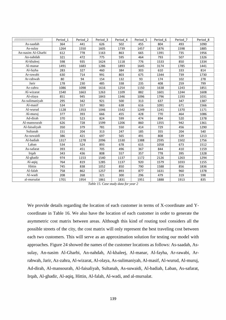
139

////////////////////////////// Period_1 Period_2 Period_3 Period_4 Period_5 Period_6 Period_7 Period_8

As-saadah 364 441 626 502 455 804 493 1090 As-sulay 1264 1550 1605 1739 1457 1876 1598 1885

An-nasim Al-Gharbi 612 778 1163 863 665 1391 735 1956 An-nahdah 321 472 775 595 464 793 507 1326 Al-khaleej 598 935 1624 1118 776 1533 850 1334 Al-manar 1491 1683 1286 1893 1645 3174 1785 1441 Al-fayha 283 327 460 384 303 610 333 814

Ar-rawabi 630 714 991 803 675 1344 739 1730 Ar-rabwah 80 94 154 132 93 174 102 278

Jarir 178 230 485 338 235 408 259 799 Az-zahra 1086 1098 1616 1254 1150 1638 1243 1851

Al-wizarat 1540 1663 1263 1109 882 1601 1244 1608 Al-olaya 851 945 1843 1346 1096 1796 1193 1031

As-sulimaniyah 295 342 921 500 313 637 347 1387 Al-masif 534 557 983 638 616 1091 671 1566 Al-wurud 1128 1353 1046 1542 1249 1241 1370 1171 Al-muruj 377 393 666 455 428 770 464 1086 Ad-dirah 370 523 824 599 474 894 520 1378

Al-mansourah 626 728 1599 1206 860 1355 942 1361 Al-faisaliyah 350 379 781 550 414 729 456 1290

Sultanah 151 204 313 247 185 355 204 540 As-suwaidi 386 421 697 565 491 808 539 1213 Al-badiah 1317 1278 2096 1530 1388 2595 1502 1756

Laban 534 524 893 678 615 1058 673 1512 As-safarat 393 451 705 496 367 844 410 1159

Irqah 343 436 808 557 357 778 395 1328 Al-ghadir 974 1153 1540 1137 1172 2126 1263 1294 Al-aqiq 764 819 1285 1137 920 1579 1033 1155 Hittin 745 838 1052 850 790 1588 856 1836

Al-falah 758 862 1257 893 877 1631 960 1378 Al-wadi 208 268 321 300 296 479 319 598

al-mursalat 1701 1954 1861 1831 1951 1888 1913 835 Table 15. Case study data for year 2

We provide details regarding the location of each customer in terms of X-coordinate and Y-

coordinate in Table 16. We also have the location of each customer in order to generate the

asymmetric cost matrix between areas. Although this kind of routing tool considers all the

possible streets of the city, the cost matrix will only represent the best traveling cost between

each two customers. This will serve as an approximation solution for testing our model with

approaches. Figure 24 showed the names of the customer locations as follows: As-saadah, As-

sulay, An-nasim Al-Gharbi, An-nahdah, Al-khaleej, Al-manar, Al-fayha, Ar-rawabi, Ar-

rabwah, Jarir, Az-zahra, Al-wizarat, Al-olaya, As-sulimaniyah, Al-masif, Al-wurud, Al-muruj,

Ad-dirah, Al-mansourah, Al-faisaliyah, Sultanah, As-suwaidi, Al-badiah, Laban, As-safarat,

Irqah, Al-ghadir, Al-aqiq, Hittin, Al-falah, Al-wadi, and al-mursalat.

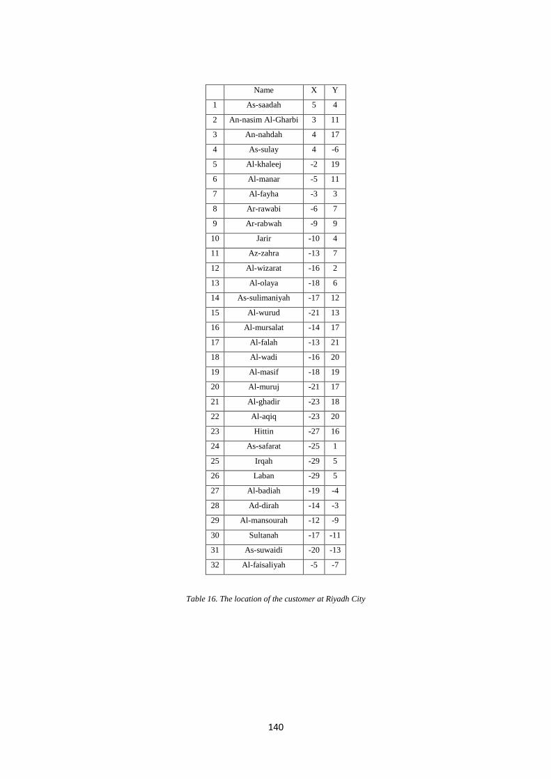
140

Name X Y

1 As-saadah 5 4

2 An-nasim Al-Gharbi 3 11

3 An-nahdah 4 17

4 As-sulay 4 -6

5 Al-khaleej -2 19

6 Al-manar -5 11

7 Al-fayha -3 3

8 Ar-rawabi -6 7

9 Ar-rabwah -9 9

10 Jarir -10 4

11 Az-zahra -13 7

12 Al-wizarat -16 2

13 Al-olaya -18 6

14 As-sulimaniyah -17 12

15 Al-wurud -21 13

16 Al-mursalat -14 17

17 Al-falah -13 21

18 Al-wadi -16 20

19 Al-masif -18 19

20 Al-muruj -21 17

21 Al-ghadir -23 18

22 Al-aqiq -23 20

23 Hittin -27 16

24 As-safarat -25 1

25 Irqah -29 5

26 Laban -29 5

27 Al-badiah -19 -4

28 Ad-dirah -14 -3

29 Al-mansourah -12 -9

30 Sultanah -17 -11

31 As-suwaidi -20 -13

32 Al-faisaliyah -5 -7

Table 16. The location of the customer at Riyadh City

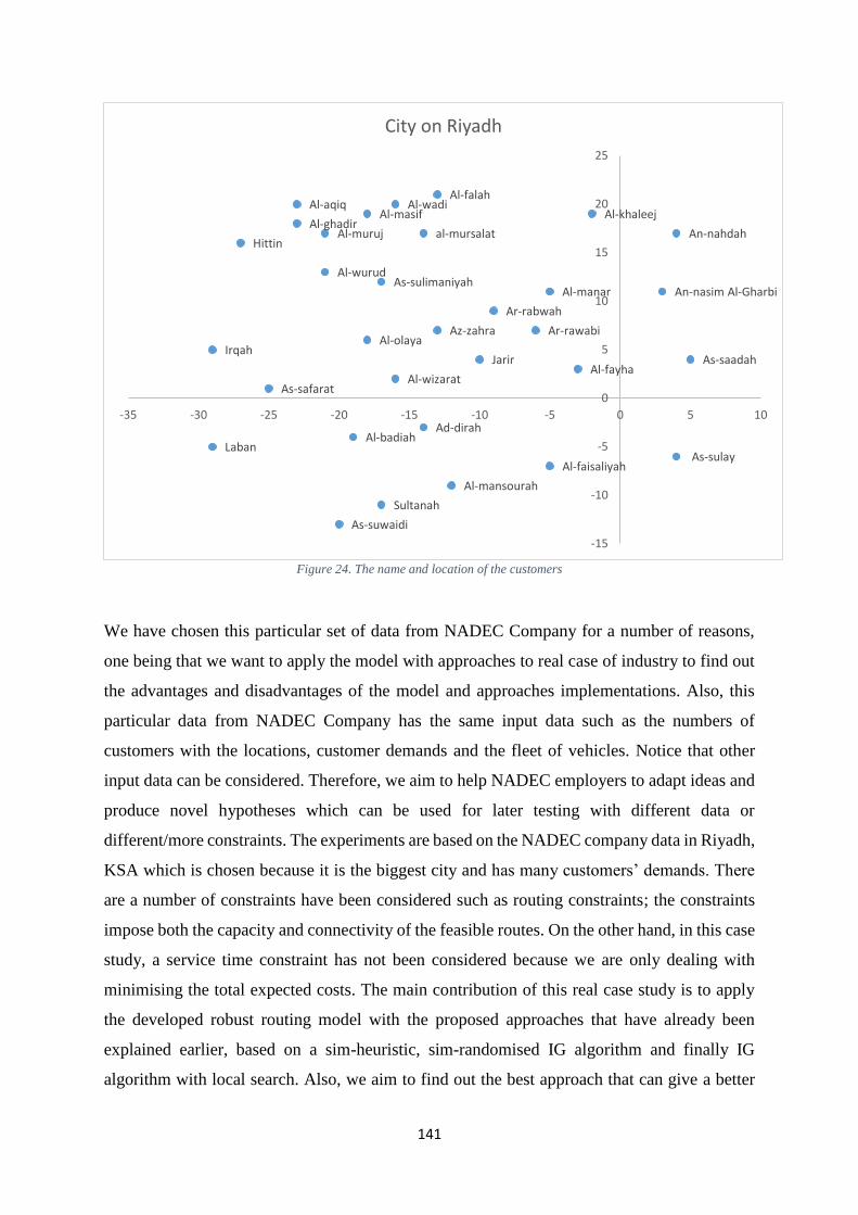
141

Figure 24. The name and location of the customers

We have chosen this particular set of data from NADEC Company for a number of reasons,

one being that we want to apply the model with approaches to real case of industry to find out

the advantages and disadvantages of the model and approaches implementations. Also, this

particular data from NADEC Company has the same input data such as the numbers of

customers with the locations, customer demands and the fleet of vehicles. Notice that other

input data can be considered. Therefore, we aim to help NADEC employers to adapt ideas and

produce novel hypotheses which can be used for later testing with different data or

different/more constraints. The experiments are based on the NADEC company data in Riyadh,

KSA which is chosen because it is the biggest city and has many customers’ demands. There

are a number of constraints have been considered such as routing constraints; the constraints

impose both the capacity and connectivity of the feasible routes. On the other hand, in this case

study, a service time constraint has not been considered because we are only dealing with

minimising the total expected costs. The main contribution of this real case study is to apply

the developed robust routing model with the proposed approaches that have already been

explained earlier, based on a sim-heuristic, sim-randomised IG algorithm and finally IG

algorithm with local search. Also, we aim to find out the best approach that can give a better

As-saadah

An-nasim Al-Gharbi

An-nahdah

As-sulay

Al-khaleej

Al-manar

Al-fayha

Ar-rawabi

Ar-rabwah

Jarir

Az-zahra

Al-wizarat

Al-olaya

As-sulimaniyahAl-wurud

al-mursalat

Al-falahAl-wadi

Al-masif

Al-murujAl-ghadir

Al-aqiq

Hittin

As-safarat

Irqah

Laban Al-badiah

Ad-dirah

Al-mansourah

Sultanah

As-suwaidi

Al-faisaliyah

-15

-10

-5

0

5

10

15

20

25

-35 -30 -25 -20 -15 -10 -5 0 5 10

City on Riyadh

142

result in terms of reducing expected total transportation costs. The algorithms are executed

using data from a company that distributes prepared food.

§6.4 Computational results

In the performed experiments, we implemented the developed robust routing model and

proposed algorithms, namely sim-heuristic with robustness, sim-Randomised with robustness

and finally sim-heuristic with robustness and IG with local search by using the instances and

the % improvement equation in section 3.6. We compared the performance of an IG algorithm

with local search (in section 5) against the best performing algorithms for both sim-heuristic

with robustness (in section 3) and sim-randomised IG with robustness (in section 4). Tables

21, 22, and 23 presented the computational results for the developed model presented in chapter

3 and proposed algorithms presented in chapter 3, 4 and 5 in which we considered the

minimisation of the expected total costs. The tables reported the results obtained for the

NADEC Company over ten runs and each table has five columns as follows; the first column

represented the names of the best solution period for total demand, the second column showed

the number of the vehicles that has been used during the service, the third column represented

the fixed cost, and the fourth column represented the expected variable cost. The last column

was the expected total cost of each period. In order to compare the solutions generated by the

company’s data, we implemented each approach in an individual table.

In Table 17, the detailed results generated by the first approach, which is sim-heuristic with

robustness, are presented. Table 18 showed the results of applied sim-randomised IG algorithm

with robustness. In Table 19, the detailed results generated by the final approach, which is sim-

heuristic with robustness and IG algorithm with local search are presented. Also, the number

of the vehicles has been presented in each of the tables. In each table, the best solution for each

approach is composed of three main parts including - fixed costs, expected variable costs and

expected total costs that are obtained by these approaches. Also, each row in the tables

represents a different period such as best solution period 1, and each period contains 13 weeks.

In these tables, we present the best solutions achieved after 10 runs. So far, the company used

different types of vehicles for each period which are described in each table. For example, the

company assigned 10, 10, 15, 15, 10, 20, 15, and 25 vehicles for period 1, 2, 3, 4, 5, 6, 7, and

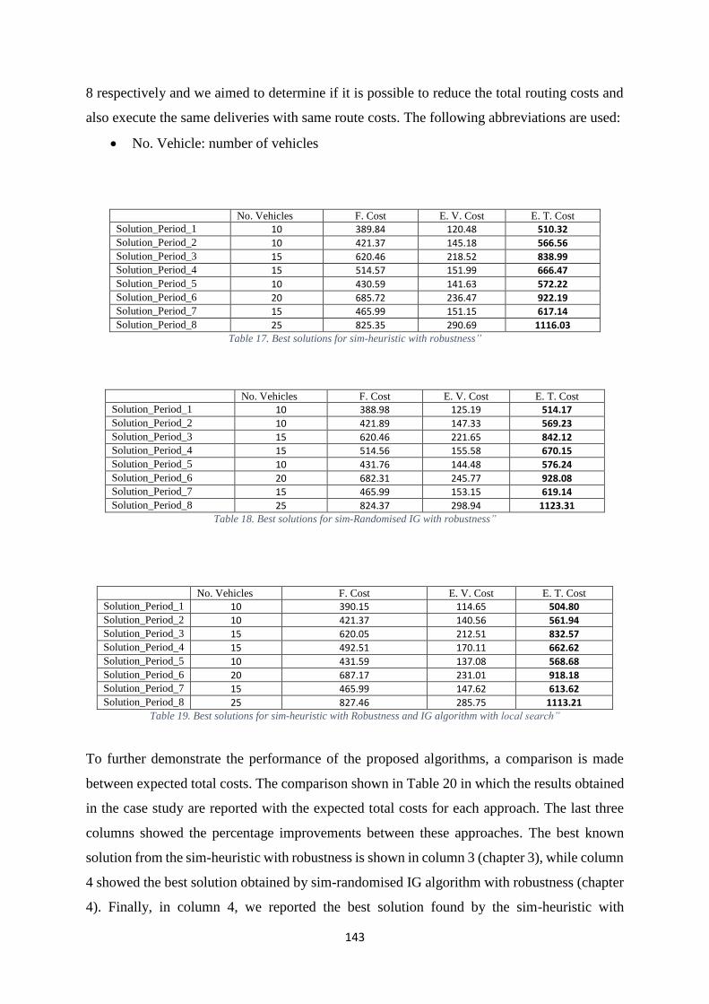
143

8 respectively and we aimed to determine if it is possible to reduce the total routing costs and

also execute the same deliveries with same route costs. The following abbreviations are used:

No. Vehicle: number of vehicles

No. Vehicles F. Cost E. V. Cost E. T. Cost

Solution_Period_1 10 389.84 120.48 510.32

Solution_Period_2 10 421.37 145.18 566.56

Solution_Period_3 15 620.46 218.52 838.99

Solution_Period_4 15 514.57 151.99 666.47

Solution_Period_5 10 430.59 141.63 572.22

Solution_Period_6 20 685.72 236.47 922.19

Solution_Period_7 15 465.99 151.15 617.14

Solution_Period_8 25 825.35 290.69 1116.03

Table 17. Best solutions for sim-heuristic with robustness”

No. Vehicles F. Cost E. V. Cost E. T. Cost

Solution_Period_1 10 388.98 125.19 514.17

Solution_Period_2 10 421.89 147.33 569.23

Solution_Period_3 15 620.46 221.65 842.12

Solution_Period_4 15 514.56 155.58 670.15

Solution_Period_5 10 431.76 144.48 576.24

Solution_Period_6 20 682.31 245.77 928.08

Solution_Period_7 15 465.99 153.15 619.14

Solution_Period_8 25 824.37 298.94 1123.31

Table 18. Best solutions for sim-Randomised IG with robustness”

No. Vehicles F. Cost E. V. Cost E. T. Cost

Solution_Period_1 10 390.15 114.65 504.80

Solution_Period_2 10 421.37 140.56 561.94

Solution_Period_3 15 620.05 212.51 832.57

Solution_Period_4 15 492.51 170.11 662.62

Solution_Period_5 10 431.59 137.08 568.68

Solution_Period_6 20 687.17 231.01 918.18

Solution_Period_7 15 465.99 147.62 613.62

Solution_Period_8 25 827.46 285.75 1113.21

Table 19. Best solutions for sim-heuristic with Robustness and IG algorithm with local search”

To further demonstrate the performance of the proposed algorithms, a comparison is made

between expected total costs. The comparison shown in Table 20 in which the results obtained

in the case study are reported with the expected total costs for each approach. The last three

columns showed the percentage improvements between these approaches. The best known

solution from the sim-heuristic with robustness is shown in column 3 (chapter 3), while column

4 showed the best solution obtained by sim-randomised IG algorithm with robustness (chapter

4). Finally, in column 4, we reported the best solution found by the sim-heuristic with

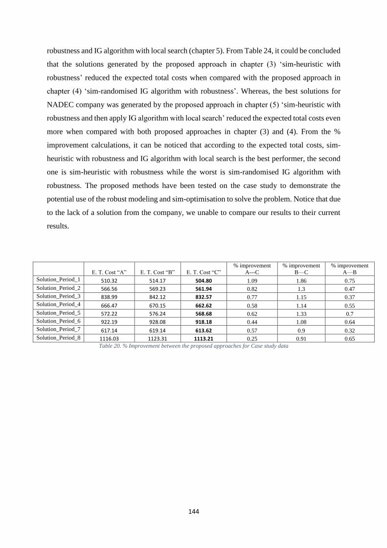
144

robustness and IG algorithm with local search (chapter 5). From Table 24, it could be concluded

that the solutions generated by the proposed approach in chapter (3) ‘sim-heuristic with

robustness’ reduced the expected total costs when compared with the proposed approach in

chapter (4) ‘sim-randomised IG algorithm with robustness’. Whereas, the best solutions for

NADEC company was generated by the proposed approach in chapter (5) ‘sim-heuristic with

robustness and then apply IG algorithm with local search’ reduced the expected total costs even

more when compared with both proposed approaches in chapter (3) and (4). From the %

improvement calculations, it can be noticed that according to the expected total costs, sim-

heuristic with robustness and IG algorithm with local search is the best performer, the second

one is sim-heuristic with robustness while the worst is sim-randomised IG algorithm with

robustness. The proposed methods have been tested on the case study to demonstrate the

potential use of the robust modeling and sim-optimisation to solve the problem. Notice that due

to the lack of a solution from the company, we unable to compare our results to their current

results.

E. T. Cost “A” E. T. Cost “B” E. T. Cost “C”

% improvement

A---C

% improvement

B—C

% improvement

A—B

Solution_Period_1 510.32 514.17 504.80 1.09 1.86 0.75

Solution_Period_2 566.56 569.23 561.94 0.82 1.3 0.47

Solution_Period_3 838.99 842.12 832.57 0.77 1.15 0.37

Solution_Period_4 666.47 670.15 662.62 0.58 1.14 0.55

Solution_Period_5 572.22 576.24 568.68 0.62 1.33 0.7

Solution_Period_6 922.19 928.08 918.18 0.44 1.08 0.64

Solution_Period_7 617.14 619.14 613.62 0.57 0.9 0.32

Solution_Period_8 1116.03 1123.31 1113.21 0.25 0.91 0.65

Table 20. % Improvement between the proposed approaches for Case study data

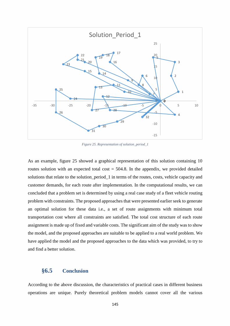
145

Figure 25. Representation of solution_period_1

As an example, figure 25 showed a graphical representation of this solution containing 10

routes solution with an expected total cost = 504.8. In the appendix, we provided detailed

solutions that relate to the solution_period_1 in terms of the routes, costs, vehicle capacity and

customer demands, for each route after implementation. In the computational results, we can

concluded that a problem set is determined by using a real case study of a fleet vehicle routing

problem with constraints. The proposed approaches that were presented earlier seek to generate

an optimal solution for these data i.e., a set of route assignments with minimum total

transportation cost where all constraints are satisfied. The total cost structure of each route

assignment is made up of fixed and variable costs. The significant aim of the study was to show

the model, and the proposed approaches are suitable to be applied to a real world problem. We

have applied the model and the proposed approaches to the data which was provided, to try to

and find a better solution.

§6.5 Conclusion

According to the above discussion, the characteristics of practical cases in different business

operations are unique. Purely theoretical problem models cannot cover all the various

0

5

3

2

1

0

16

1718

19

14

0

9

2021

22

23

15

10

024

25

26

31

30

29

0

4

28

12

0

7

8

6

0

1113

27

0

32

0

-15

-10

-5

0

5

10

15

20

25

-35 -30 -25 -20 -15 -10 -5 0 5 10

Solution_Period_1

146

restrictions found in real situations. Therefore, models designed are based on different business

scenarios. The complexity is increased when different/many constraints are involved; then, a

heuristic algorithm is consider as one of the best choices to implement and develop and thus

solve these specific problems. Due to differences in the details of the data, experiments cannot

be performed on a benchmark problem set. Notice that we can include any new constraints

depending on the real case study situation, such as time windows or traffic, and solve the

problem in order to find the best solution of the case study. The main step is that we have to

formulate the model and constraints to include these new constraints. Since the decision maker

is able to handle diverse routing extensions, it should be easy to roll-out to other companies

facing similar real-world problems. Of course, the most straightforward step would be to go to

other companies having a similar business model. Catering companies also seem to be a natural

extension as they also handle different types of vehicles and exigent customers with several

requirements. Nevertheless, the potential savings are of a lower size as the amount and intensity

of the deliveries is not the same. Other companies to which this approach could be rolled-out

may be found in the waste collection business or big food producers that have their distribution

process internalised.

The main essential of using the case study was to explore the effectiveness of quality

improvement and inform the development of both the model with the approaches that were

explained earlier. The case study is a well-established way in organisational researches that are

more frequently used in organisational transportation research such as food distribution. In this

chapter, we presented a real case study faced by a food distribution company in Saudi. Also,

we discuss a real-data implementation of the proposed model with all heuristics which were

presented earlier in the thesis. The experiments are based on the NADEC company data in

Riyadh, KSA which is chosen because of it is the biggest city that has many customers’

demands. We have tested all proposed algorithms for NADEC information. This work shows

some challenges to design and implementation of routing algorithms for automatising real data

company distribution processes. I wish through these results it will possible to support NADEC

Company to provide a technique for generating a set of alternative routing solutions with

different features, and improve the NADEC Company profits.

147

Chapter 7 : Conclusion and future research

§7.1 Conclusion

This thesis examined the stochastic variation of the VRP, the VRPSD. VRPSD is a very

important and present-day problem, impacting costs and productivity in industrial distribution

systems. VRPSD is an intensive study in which there is uncertainty in customer’s demands.

The location of each customer is known in advance and before the vehicle starts to serve them,

but the real demand is known when the vehicle arrives at the customer’s location. This makes

the problem more suitable for certain real-life cases in which the customers’ demands are not

known in advance, but can only be modelled by a random variable and are known when the

vehicle arrives at the customer’s location. The objective is to minimise the expected total costs

of the VRPSD. This thesis dealt with several approaches for solving VRPSD. These approaches

focus on three main axes: robust routing model, biased randomisation and integration of

randomised heuristics with simulation. An extensive literature review was carried out, focusing

on describing the evolution of the main contribution from previous works.

Our main contributions to scientific understanding begin in Chapter 3, where we set out how

exactly we intend to improve on the existing methods of heuristics to solve VRPSD. The study

examined robust routing model and sim-heuristic for solving VRPSD. The a-priori route is

generated by using CWS heuristic. The major contribution is the formulation of the robust

routing model that minimises the deviations from the a-priori route and the use of a sim-

heuristic that integrates MCS inside biased randomised heuristic to provide a near-optimal

solution and demonstrate its effectiveness by obtaining high-quality solutions for VRPSD. We

aimed to build robust solutions by developing the robust routing model and sim-heuristics

approach in order to minimise the expected total cost for VRPSD, and also to design

experiments to measure performance with respect to the instances chosen from the literature.

The vehicle maximum capacity is accounted for when deigning the routes. In terms of the

computational analysis, the model with sim-heuristic provided robust solutions for uncertain

scenario. Also, the robustness of a solution against the uncertain data can be achieved by

making the solution feasible for any customer demand defined in the uncertainty set.

Furthermore, our solutions were compared with other solution methods thus the computational

148

results obviously showed that the robust routing model is able to provide good quality solutions

for almost all instances. In addition, the results have shown that the robust routing model and

sim-heuristics are effective and efficient in all 55 instances when compared with literature

results.

The primary contribution of chapter 4 is the design and implementation of the randomised IG

algorithm with MCS and robustness to solve VRPSD. This method is based on an initial

solution that is generated by a CWS heuristic. We adapted IG for solving deterministic case

and MCS integrated with randomised version of IG to solve VRPSD. The integration between

the randomised IG algorithm with MCS and robustness produced a sequence of solutions by

iterating over greedy constructive heuristics using two main phases iteratively: named

destruction and construction. The objective function is to minimise the overall transportation

cost and it is defined in the robust routing model with constraints which are explained in chapter

3. There are two stages in order to solve VRPSD; in the first stage, an IG algorithm is used in

order to find the optimal solution for deterministic VRP before adding the randomisation into

the IG algorithm as an extension work in the deterministic case. The next stage has one step

further to develop an IG algorithm as well as to solve the problem in the stochastic case, which

is VRPSD, using a proposed a randomised IG with MCS and robustness. Both stages have been

used in the well-known benchmark problem and the final solutions for VRPSD are compared

with previous solutions in chapter 3. To conclude that this algorithm requires several steps;

firstly, an initial solution generated using CWS. Secondly, biased randomised integrated inside

the IG algorithm implementation and biased randomised function based on the geometric

distribution, used for sorting the customer’s demand depending on the probability. Finally, it

generates random variables to estimate the expected total cost by using MCS.

Another approach that has the potential to solve VRPSD is to apply an IG algorithm with local

search that we considered in chapter 5. The approach we employed in chapter 5 is more typical

because it has been designed in order to improve the solutions. Therefore, the aim of the final

contribution was to improve the final solutions using the IG algorithm with local search. The

IG algorithm with local search procedure is straightforwardly added to the final solutions that

were obtained using sim-heuristic with robustness, in order to bring about further significant

improvements to the VRPSD solution. The idea itself is very interesting since the combination

149

can produce good solutions. To conclude, these approaches focused on three main parts: robust

routing model, the integration of randomised heuristics with MCS, and the application of the

IG algorithm with local search. From the computational results, implementing the IG algorithm

with local search improved most of the solutions, as shown in experimental results section.

Also, we demonstrated the effectiveness of our approaches by showing the computational

results and comparing with the results of the previous chapters 3 and 4.

Finally, chapter 6 presented a real case study from NADEC Company in the Riyadh city in

order to implement the robust routing model; all the approaches have already been proposed

earlier in chapters 3, 4, and 5 and the results compared with each other. Also, it is to find out

the best approach that can give better results in terms of reducing total transportation costs.

The algorithms are executed using data from a company that distributes prepared food and we

discussed several results in a real case study by using different approaches. The computational

results presented in chapter 6 indicated that the results obtained by the approach proposed in

chapter 5 are superior to the other results obtained by the approach proposed in chapter 3 and

4.

150

§7.2 Extensions and future work

Whilst this thesis does show very interesting ideas to solve VRPSD and the computational

results obtained are good quality solutions. It is clear from the computational effort that there

are opportunities to implement different algorithm solutions in future work.

In this thesis, we have shown how the model and the approaches can successfully be

applied to VRPSD. One interesting future research is testing different stochastic models

with these approaches in order to improve and compare the solutions of the VRPSD.

Another research line is to consider multi-objective optimisation models that take into

account different objectives such as minimising the total expected cost and the number

of vehicles simultaneously. Also, other objective can be considered.

One direction for future research could be to use these proposed algorithms to develop

efficient algorithms to solve similar kinds of problems with different/special

characteristics. In addition, there is the opportunity to implement the model with the

proposed algorithms with different constraints to improve the solution quality. Looking

to the future research, the problem could be complicated by the application of time

windows for each customer. Time can play an important role to improve the

transportation cost when we combine it with stochastic demand. Note that a penalty for

late/early arrivals or the extra time cost of the driver, can be part of the expected cost

when time windows and/or stochastic service time are taken into consideration. In

addition, it can be assumed that a large number of problems can use the model with the

algorithms to improve the quality of solutions, such as inventory routing problems and

location routing problem.

One of the future research routes is to include the time-dependency of the travel times

in order to serve customer demand. In real-life applications, it is essential to consider

time-dependent travel times since speeds vary throughout the day due to events like

accidents or congestion during the rush hours. By including this property, we have both

stochastic and dynamic travel times. This structure requires adjustments in the

algorithms with respect to the distributions of the arrival times.

A study of different variations of the problem: one of the interesting future research

routes is to consider stochastic customers whilst taking into account stochastic

demands. Each customer 𝑖 has a probability (𝑃𝑖) of presence and probability (1 − 𝑃𝑖)

151

of absent. Because of uncertainty, it may not be possible to follow vehicle routes as

planned. The problem is solved in two stages. In a first stage, planned collection routes

are designed. In a second stage, when the set of present customers is known, these routes

are followed as planned by skipping the absent customers. Whenever the vehicle

capacity is exceeded, the recourse actions can be applied e.g., the vehicle travels back

to the depot and resumes its collections along the planned route.

One potential area of interesting future research is to consider other biased (non-

symmetric) probabilistic distributions to measure performance and its impact on results,

while we proposed algorithms that are based on a biased-randomised selection of

elements inside of heuristics.

Based on the literature review chapters, the stochastic consideration is not limited to

customer demand and time, but also includes other side considerations such as road

weather conditions and working shifts. Apart from the findings, one of the significant

future research studies is to apply the proposed approaches when considering these

variations.

Another possibility of the future work for improving the quality of the solutions

achieved by the randomised IG algorithm with MCS, is applying cache and splitting

technique. Additionally, the algorithm incorporates some memory capabilities which

are provided in a hash table of the best-known routes and specific splitting techniques,

which are based on the geometrical properties of intermediate solutions. As (Juan et al.,

2011b) reported that the joint use of memory capabilities and splitting techniques

contributes to a significant improvement in the overall performance of the hybrid CWS-

MCS base algorithm.

Another possibility of future work for improving the quality of the solutions achieved

by the randomised IG algorithm with MCS, is to apply the biased randomisation

technique at the phase of generating the initial solution. From the initial solution, the

customer’s demand with high probability can be removed and reinserted back. This

could lead to an improvement in the solution from the beginning. Also, local search can

be applied after the construction phase in order to improve the solution from the IG

algorithm procedure before applying MCS.

152

Chapter 8 : References

Aarts, E., and Lenstra, J, K. (1997). Local search in combinatorial optimization. John Wiley &

Sons, Inc, New York, NK, USA.

Amorim, P., Parragh, S, N., Sperandio, F., Almada-Lobo, B. (2014). A rich vehicle routing

problem dealing with perishable food: a case study. Hindawi Publishing Corporation,

Discrete Dynamics in Nature and Society. Sociedad de Estadística e Investigación

Operativa 22:489–508.

Amponsah, S. K., & Salhi, S. (2004). The investigation of a class of capacitated arc routing

problems: The collection of garbage in developing countries. Waste Management, 24,

711–721.

Ak. A., and Erera, A, L. (2007). A paired vehicle recourse strategy for the vehicle routing

problem with stochastic demand. Transportation Science, 41(2): 222-237.

Andradottir, S. (1998). A review of simulation optimisation techniques. Proceedings of the

Winter Simulation Conference.

Augerat, P., Belenguer. J. M., Benavent, E., Corbern, A., Naddef, D., and Rinaldi, G. (1995).

Computational results with a branch and cut code for the capacitated vehicle routing

problem. Research report 949-m. 25 pages. Universite Joseph Fourier, Grenoble,

France.

Avci, M., & Topaloglu, S. (2015). An adaptive local search algorithm for vehicle routing

problem with simultaneous and mixed pickups and deliveries. Computer & Industrial

Engineering, 83, 15–29.

Balaprakash, P., Birattari, M., Stützle, T., & Dorigo, M. (2015). Estimation-based

metaheuristics for the single vehicle routing with stochastic demands and customers.

Computational Optimization and Applications, 463–487.

Bastian, C., Alexander. H. G., Kan, R. (1992). The stochastic vehicle routing problem revisited,

European Journal of Opertational Research 56, 407–412.

Bastian, C. and Rinnooy, K. (1992). The stochastic vehicle routing problem revisited. European

Journal of Operational Research, 56(3):407–412.

Berhan, E., Beshah, B., Kitaw, D., & Abraham, A. (2014a). Stochastic vehicle routing problem:

a literature survey. Journal of Information & Knowledge Management, Vol. 13, No. 3.

World Scientific Publishing Company.

Berhan, E., Kromer, P., Kitaw, D., & Abraham, A., Snasel. V. (2014). Solving stochastic

vehicle routing problem with real simultaneous pickup and delivery using differential

evolution. Springer International Publishing. 187–200.

Bertsimas, D. J. (1991). A vehicle routing problem with stochastic demand. Institue for

Operations Research and the Management Sciences (INFORMS). 40(3): 574-585.

Bektas, T., and Laporte, G. (2011). The pollution-routing problem. Transportation Research

Part B 45: 1232–1250.

Bianchi, L., Dorigo, M., Gambardella, L, M., & Gutjahr, W. J. (2009). A survey on

metaheuristics for stochastic combinatorial optimization. Journal Natural Computing: an

International Journal. Springer Science and Business Media B.V. Vol. 8. Issue 2, 239-287.

Bianchi, L., Birattari, M., Chiarandini, M,. Manfrin, M., Mastrolilli, M., Paquete, L., Rossi-

Doria, Oliva., & Schiavinotto, T. (2004). Metaheuristics for the vehicle routing problem

with stochastic demands. Springer-Verlag Berlin Heidelbery, Pp. 450-460.

Bianchi, L., Birattari, M., Chiarandini, M., Manfrin, M., Mastrolli, M., Paquete, L., Rossi-

Doria, Olivia., Schiavinotto, T. (2006). Hybird metaheuristics for the vehicle routing

problem with stochastic demands. J. Math Model Algorithms. 5(1):91-110.

Biesinger, B., Hu, B., Raidl, R, G. (2015). A variable neighborhood search for the generalized

153

vehicle routing problem with stochastic demands, Springer International Publishing

Switzerland. 48–60.

Bjerring. J. H. (2010). The Dial-A-Ride problem and exploiting knowledge about future

customer requests. Master’s Thesis in Mathematics- Economics.

Bozorgirad, M. A., Logendran, R. (2015). A comparison of local search algorithms with

population-based algorithms in hybrid flow shop scheduling problems with realistic

characteristics. International Journal of Advanced Manufacturing Technology. Vol. 83.

Issue 5. 1135-1151.

Braysy, O., Gendreau, M. (2005). Vehicle routing problem with time windows , Part I : route

construction and local search algorithms. Transportation Science. INFORM. 39(1), 104–

118.

Braysy, O., Gendreau, M. (2005a). Vehicle routing problem with time windows, Part II :

metaheuristics, Transportation Science. 39(1), 119–139.

Bresina, J. L. (1996). Heuristic-Biased stochastic sampling. Proceeding AAAI’96 Proceedings

of the Thirteenth National Conference on Artificial Intelligence.Vol 1, 271–278.

Cabrera G, Juan A, Lazaro D, Marques J, Proskurnia I. (2014). A simulation-optimization

approach to deploy internet services in large-scale systems with userprovided resources.

Simulation: Transactions of the Society Modeling and Simulation International.

90(6):644–59.

Cáceres-cruz, J., Riera, D., Buil, R., & Juan, A. A. (2013). Applying a savings algorithm for

solving a rich vehicle routing problem in a real urban context. 5th International

Conference on Applied Operational Research, 5, 84–92.

Cáceres-cruz, (2013). Randomized algorithms for rich vehicle routing problems : From a

specialized approach to a generic methodology. PhD thesis.

Chalghoumi, S., Ladhari, T. (2015). Iterated greedy local search and simulated annealing

algorithms for the two-machine flowshop scheduling problem . International Conference

On automation, Control, Engineering and Computer Science.

Chandu, D, P. (2015). Improved greedy algorithm for set covering problem. SSRG

International Journal of computer Science and engineering (SSRG-IJCSE).

Chang, M. S. (2005). A vehicle routing problem with time windows and stochastic demands.

Journal of the Chinese Institute of Engineers. Vol. 28, No, 5. 783-794

Chepuri, K., and Homem-De-Mello, T. (2004). Solving the vehicle routing problem with

stochastic demand using the Cross-Entropy method. Annuals of Operations Research.

134, 154-181.

Christiansen, C. H., & Lysgaard, J. (2007). A branch-and-price algorithm for the capacitated

vehicle routing problem with stochastic demands, Operationas Research Letters 35, 773–

781.

Christiansen, C. H., Lysgaard, J., & Wøhlk, S. (2009). A Branch-and-Price algorithm for the

capacitated arc routing problem with stochastic demands. Operations Research Letters,

37(6), 392–398.

Clarke, G. and J.W. Wright. (1964). Scheduling of vehicles from a central depot to a number

of delivery points. Operations Research 12, 568−581.

Cordeau, J, F., Laporte, G., Savelsbergh, M, W, P., Vigo, D. (2007). Vehicle routing.

Handbook in OR & MS, Vol. 14.

Cordeau, J. F., Gendreau, M., Laporte, G., Potvin, J-Y., Semet, F. (2002). A guide to vehicle

routing heuristics. Journal of the Operational Research Society., 53(5), 512–522.

Dantzig, G. and Ramser, J. (1959). The truck dispatching problem. Management Science,

6(1):80-91.

Dror, M., & Trudeau, P. (1986). Stochastic vehicle routing with modified savings algorithm.

European Journal of Operational Research, 23, 228–235.

154

Dror, M., Laporte, G., Trudeau, P. (1989). Vehicle routing problem with stochastic demand:

properties and solution frameworks. Transportation Science. Vol. 23, No. 3.

Eksioglu, B., Vural, A, V., and Reisman, A. (2009). The vehicle routing problem: A taxonomic

review. Computers and Industrial Engineering, 57(4), 1472-1483.

Erbao, C., Mingyony, L., Hongming, Y. (2014). Open vehicle routing problem with demand

uncertainty and its robust strategies. Expert systems with applications 41. 3569-3575.

Festa, P., & Resende, M. G. C. (2009). An annotated bibliography of GRASP- Part I :

algorithms. International Transactions in Operational Research, 16, 1–24.

Fu, M, C., Glover, F, W., April, J. (2005). Simulation optimization: A review, new

developments and applications. Proceedings of the Winter Simulation Conference. M. E.

Kuhl, N. M. Steiger, F. B. Armstrong, and J. A. Joines, eds.

Gauvin, C., Desaulniers, G., and Gendreau, M. (2014). A branch-cut-and-price algorithm for

the vehicle routing problem with stochastic demands. Computers & operations Research,

50(0): 141-153

Gendreau, M., Laporte, G., Seguin, R. (1996a). Stochastic vehicle routing. European Journal

of Operational Research 88, 3-12.

Gendreau, M., Laporte, G., & Séguin, R. (1995). An exact algorithm for the vehicle routing

problem with stochastic demands and customers. Transportation Science, Vol. 29, No. 2,

143-155, INFORM.

Gendreau, M., Laporte, G., & Séguin, R. (1996). A tabu search heuristic for the vehicle routing

problem with stochastic demands and customers. Operations Research, 44(3), 469–477.

Gendreau, M., Potvin, J., & Braysy, O., Hasle, G., Lokketangen, A. (2008). Metaheuristics for

the vehicle routing problem and its extensions : A categorized bibliography. Springer

Science + Business Meddia, LLC.

Gendreau, M., Jabali, O., and Rei, W. (2014). Stochastic vehicle routing problems. In Toth, P.

and Vigo, D., editors, vehicle routing: problems, methods, and applications, Second

Edition, pages 213-239. Society for Industrial and Applied Mathematics.

Glover, F., Kelly, J. P., Laguna, M. (1999). New advances for wedding optimization and

simulation. Proceedings of the 1999 Winter Simulation Conference.

Glover, F., Kelly, J, P., Lagune, M. (1996). New advance and applications of combining

simulation and optimisation. Proceedings of the 1996 Winter Simulation Conference.

Gonzalez S, Juan A, Riera D, Elizondo M, Fonseca P. (2012). Sim-RandSHARP: A hybrid

algorithm for solving the arc routing problem with stochastic demands. In: Proceedings

of the 2012 winter simulation conference. p. 1–11.

Goodson, J. C. (2015). A priori policy evaluation and cyclic-order-based simulated annealing

for the multi-compartment vehicle routing problem with stochastic demands. European

Journal of Operational Research, 241, 361–369.

Goodson, J. C., Ohlmann, J. W., & Thomas, B. W. (2012). Cyclic-order neighborhoods with

application to the vehicle routing problem with stochastic demand. European Journal of

Operational Research, 217(2), 312–323.

Gounaris, C. E., Wiesemann, W., and Floudas, C, A. (2013). The robust capacitated vehicle

routing problem under demand uncertainty. Operations research, 61(3):677-693.

Groër, C., Golden, B., & Wasil, E. (2010). A library of local search heuristics for the vehicle

routing problem. Math. Prog. Comp. 2, 79–101.

Hajer, A., & Talel, L. (2013). Iterated local search and iterated greedy local search for two

machines permutation flowshop scheduling problem with time lag. IEEE.

Hansen, P., Mladenovic, N., & Perez, J. A. M. (2010). Variable neighbourhood search:

methods and applications. Annuals of Operation Research, 175, 367–407.

Haugland, D., Ho, S., Laporte, G. (2007). Designing delivery districts for the vehicle routing

problem with stochastic demands. Eur J Oper Res 180:997-1010.

155

Hemmelmayr, V., Doerner, K. F., Hartl, R. F., & Savelsbergh, M. W. P. (2010). Vendor

managed inventory for environments with stochastic product usage. European Journal of

Operational Research, 202(3), 686–695.

Hjorring, C., & Holt, J. (1999). New optimality cuts for a single-vehicle stochastic routing

problem. Annuals of Operations Research, 86, 569–584.

Huerta-muñoz, D. L., Rios-Mercado, R, Z., Ruiz, R. (2012). An iterated greedy heuristic for a

market segmentation problem with multiple attributes. Report Number: PISIS-2012-02,

Affiliation: Graduate Program in Systems Engineering, UANL.

Ibaraki, T., Kubo, M., Masuda, T., Uno, T., Yagiura, M. (2001). Effective local search

algorithms for the vehicle routing problem with general time windows constraints. 4th

Metaheuristics International Conference. Porto, Portugal, July 16-20, 2001.

Iori, M., & Riera-ledesma, J. (2015). Exact algorithms for the double vehicle routing problem

with multiple stacks. Computers and Operation Research, 63, 83–101.

Ismail, HZ., and Irhamah. I. (2008). Solving the vehicle routing problem with stochastic

demands via hybrid genetic algorithm-tabu search. Journal of Mathematics and Statistics,

4(3), 161-167.

Jabali, O., Van Woensel, T., de Kok, A.G. (2012). Analysis of travel times and CO2 emissions

in time-dependent vehicle routing. Production and Operations Management 21, 1060–

1074.

Jabali, O., Rei, W., Gendreau, M., & Laporte, G. (2014). Partial-route inequalities for the multi-

vehicle routing problem with stochastic demands. Discrete Applied Mathematics, 177,

121–136.

Juan, A. A., Adelantado, F., Faulin, J., Grasman, S. E., & Montoya-Torres, J. R. (2009).

Solving the capacitated vehicle routing problem with maximum traveling distance and

service time requirements: An approach based on Monte Carlo simulation. Proceedings -

Winter Simulation Conference, 2467–2475.

Juan, A. A., Barrios, B. B., Vallada, E., Riera, D., & Jorba, J. (2014a). SIM-ESP: A simheuristic

algorithm for solving the permutation flow shop problem with stochastic processing times.

Simulation modelling practice and theory. 46,101–117.

Juan, A. A., Cáceres-Cruz, J., González-Martín, S., Riera, D., & Barrios, B. B. (2014). Biased

randomization of classical heuristics. Encyclopedia of Business Analytics and

Optimization, Vol. 1, 314–324.

Juan, A. A., Faulin, J., Ferrer, A., Lourenço, H. R., & Barrios, B. (2013b). MIRHA : multi-start

biased randomization of heuristics with adaptive local search for solving non-smooth

routing problems. 21,109–132.

Juan, A. A., Faulin, J., Grasman, S. E., Rabe, M., & Figueira, G. (2015). A review of

simheuristics: Extending metaheuristics to deal with stochastic combinatorial

optimization problems. Operations Research Perspectives, 2, 62–72.

Juan, A. A., Faulin, J., Jorba, J., Caceres, J., & Marquès, J. M. (2013a). Using parallel &

distributed computing for real-time solving of vehicle routing problems with stochastic

demands. Ann Oper Res, 207, 43–65.

Juan, A. A., Faulin, J., Ruiz, R. N., Barrios, B., & Caballé, S. (2010). The SR-GCWS hybrid

algorithm for solving the capacitated vehicle routing problem. Applied Soft Computing

10, 215-224.

Juan, A. A., Grasman, S. E., Caceres-Cruz, J., & Bektas, T. (2014b). A simheuristic algorithm

for the single-period stochastic inventory-routing problem with stock-outs. Simulation

Modelling Practice and Theory, 46, 40–52.

Juan, A. A., Lourenc, H. R., Mateo, M., & Castell, Q., Barrios, B, B. (2012). ILS-ESP : an

efficient, simple, and parameter-free algorithm for solving the permutation flow-shop

problem. European Journal of Operational Research.

156

Juan, A., Faulin, J., Grasman, S., Riera, D., Marull, J., & Mendez, C. (2011a). Using safety

stocks and simulation to solve the vehicle routing problem with stochastic demands.

Transportation Research Part C, 19(5), 751–765.

Juan, A., Faulin, J., Jorba, J., Riera, D., Masip, D., & Barrios, B. (2011b). On the use of monte

carlo simulation, cache and splitting techniques to improve the Clarke and Wright savings

heuristics. Journal of the Operational Research Society, 62(62), 1085–1097.

Juan, A., Faulin, J., Riera, D., Caceres, J., & Grasman, S. (2011c). A simulation-based

algorithm for solving the vehicle routing problem with stochastic demands. Proc. Of the

VII ALIO-EURO-Workshop on Applied Combinatorial Optimsation. 133–136.

Juan, A., Rabe, M. (2013). Combining simulation with heuristics to solve stochastic routing

and scheduling problems. In proceedings of the 15th ASIM Dedicated Conference,

Paderborn, Germany, October. 130-225.

Juan. A., Faulin. J., Perez-Bernabeu. E., Dominguez, O. (2013c). Simulation-optimsation

methods in the vehicle routing problems; a literature review and an example. Springer

lecture notes in business information processing, 145:155-124.

Laporte, G., Louveaux, F., & Mercure, H. (1992). The vehicle routing problem with stochastic

travel times. Transportation Science, Vol. 26, No. 3: 161-170.

Laporte, G., (1992). The Vehicle Routing Problem : An overview of exact and approximate

algorithms. European Journal of Operational Research, 59, 345–358.

Laporte, G., François V. L., and Luc, V., H. (2002). An integer L-shaped algorithm for the

capacitated vehicle routing problem with stochastic demands. Operations Research 50(3):

415-423.

Lee, C., Lee, K., & Park, S. (2012). Robust vehicle routing problem with deadlines and travel

time&sol;demand uncertainty. Journal of the Operational Research Society, 63, 1294-

1306.

Lei, H., Laporte, G., & Guo, B. (2011). The capacitated vehicle routing problem with stochastic

demands and time windows. Computers and Operation Research, 38(12), 1775–1783.

Li, P., He, J., Zheng, D., Huang, Y., Fan, C. (2015). Vehicle routing problem with soft time

windows based on improved genetic algorithm for fruits and vegetables distribution.

Hindawi Publishing Corporation, Discrete Dynamics in Nature and Society. 8 pages.

Long-fei, W., Le-Yuan, S. (2013). Simulation optimization : A review on theory and

applications. Acta Automatica Sinica, 39(11), 1957–1968.

Marinakis, Y., Lordanidou, G., and Marinaki, M. (2013). Particle swarm optimisation for the

vehicle routing problem with stochastic demand. Applied soft computing. 13(4); 1693-

1704.

Mendoza, J. E., Castanier, B., & Guéret, C., Medaglia, A, L., Velasco, N. (2011). Constructive

heuristics for the multicompartment vehicle routing problem with stochastic demands.

Transportation Science, 45(3), 346–363.

Mendoza, J, E., Rousseau, M, L., Villegas, J. G. (2015). A hybrid metaheuristic for the vehicle

routing problem with stochastic demand and duration constraints. Journal of Heuristics.

1-28.

Mohan, R., Gopalan, N, P. (2014). Task assignment for heterogeneous computing problems

using improved iterated greedy algorithm. I.J. Computer Network and Information

Security. 50-55.

Moghaddam, B, F., Ruiz, R., Sadjadi, S. J. (2012). Vehicle routing problem with uncertain

demand: An advanced particle swarm algorithm. Computers and Industrial Engineering,

62(1), 306–317.

Mulvey. J. M., Vanderbei. R. J., and Zenios. S. A. (1995). Robust optimization of large-scale

systems. 1995. Operations Research, vol.43, no. 2, pp. 264–281.

Mungwattana, A., Soonpracha, K., Manisri, T. (2016). A Practical case study of a

157

heterogeneous fleet vehicle routing problem with various constraints. Proceedings of the

2016 International Conference on Industrial Engineering and Operations Management

Kuala Lumpur, Malaysia, March 8-10.

Naderi, B., Rahmani, S., & Rahmani, S. (2014). A multiobjective iterated greedy algorithm for

truck scheduling in Cross-Dock problems. Hindawi Publishing Corporation, Journal of

Industrial Engineering. 12 pages.

Naderi, B., Zandieh, M., Mohammad, S., & Fatemi, T. (2009). An iterated greedy algorithm

for flexible flow lines with sequence dependent setup times to minimize total weighted

Completion Time. Journal of Industrial Engineering, 3, 33–37.

Noorizadegan, M., Galli, L., Chen, B. (2012). On the heterogeneous vehicle routing problem

under demand uncertainty. 21st International Symposium on Mathematical Programming,

Berllin, Germany. pp. 1-25.

Novoa, C., Storer, R. (2009). An approximate dynamic programming approach for the vehicle

routing problem with stochastic demands. European Journal of Operational Research,

196(2), 509–515.

Quan-Ke, P, and Ruiz, R. (2012). Local search methods for the flowshop scheduling problem

with flowtime minimisation. European Journal of Operational Research 222. (1): 31-43.

Osvald, A., Stirn, L, Z. (2008). A vehicle routing algorithm for the distribution of fresh

vegetables and similar perishable food. Journal of Food Engineering, 85, 285–295.

Oyola, J., Arntzen, H., Woodruff, D. L. (2016). The stochastic vehicle routing problem , a

literature review.

Peyró, L. F., and Ruiz, R. (2010). Iterated greedy local search methods for unrelated parallel

machine scheduling. European Journal of Operational Research, 207(1), 55–69.

Pen, Q., and Ruiz, R. (2012). Local search methods for the flowshop scheduling problem with

flowtime minimization. European Journal of Operational Research, vol. 222, issue 1,

pages 31- 43.

Pranzo, M., & Pacciarelli, D. (2015). An iterated greedy metaheuristic for the blocking job

shop scheduling problem. Journal of Heuristics, 1-25.

Prindezis, N., Kiranoudis, C. T., & Marinos-Kouris, D. (2003). A business-to-business fleet

management service provider for central food market enterprises. Journal of Food

Engineering, 60(2), 203–210.

Ribas, I., Companys, R. and Tort-Martorell, X. (2011). An iterated greedy algorithm for the

flowshop scheduling problem with blocking. OMEGA, The international Journal of

Management Science, 39(3):293–301.

Resende, M. G. C., & Ribeiro, C. C. (2010). Greedy randomized adaptive search procedures :

Advances, hybridizations, and applications. Handbook of metaheuristics. Vol. 146 of the

series International Series in Operations Research & Management Science, 283-319.

Pop, P, C., and Horvat-Marc, A. (2012). Local search heuristics for the generalized vehicle

routing problem. International conference on system modeling and optimization (ICSMO

2012) IPCSIT vol. 23. Press, Singapore.

Ruiz, R., Stutzle, T. (2005). An iterated greedy algorithm for the flowshop problem with

sequence dependent setup times. The 6th Metaheuristics International Conference, 817–

823.

Ruiz, R., Stutzle, T. (2007). A simple and effective iterated greedy algorithm for the

permutation flowshop scheduling problem. European Journal of Operational Research,

177, 2033–2049.

Savelsbergh, M. W. P. (1985). Local search in routing problems with time windows. Annuals

of Operations Research. 4(6):285-305.

Secomandi, N. (2001). A rollout policy for the vehicle routing problem with stochastic

demands. Operations Research 49 796-802.

158

Solano-charris, E., Prins, C., & Cynthia, A. (2015). Local search based metaheuristics for the

robust vehicle routing problem with discrete scenarios. Applied Soft Computing Journal,

32, 518–531.

Solomon, M.M. (1987). Algorithms for the vehicle routing and scheduling problems with time

window constraints. Operations Research 35, 254−265.

Stewart, R., & Golden, B. L. (1983). Stochastic vehicle routing : A comprehensive approach.

European Journal of Operational Research. 14, 371-385.

Sun, L., & Wang, B. (2015). Robust optimisation approach for vehicle routing problems with

uncertainty. Hindawi publishing Corporation, Mathematical Problems in Engineering, 8

pages.

Sungur, I., Ordonez, F., Dessouky, M. (2007). A robust optimization approach for the

capacitated vehicle routing problem with demand uncertainty. Transportation Science.

Vol. 44, No. 2, 193–205.

Tas, D., Dellaert, N., Woensel, T. Van., Kok, T. De. (2013). Vehicle routing problem with

stochastic travel times including soft time windows and service costs, 40, 214–224.

Talbi, E.-G. (2009). Metaheuristics from design to implementation. John Wiley & Sons, Inc.

Hoboken, New Jersey.

Tan, K. C., Cheong, C. Y., & Goh, C. K. (2007). Solving multiobjective vehicle routing

problem with stochastic demand via evolutionary computation. European Journal of

Operational Research, 177, 813–839.

Tarantilis, C. D., & Kiranoudis, C. T. (2002). Distribution of fresh meat. Journal of Food

Engineering, 51(1), 85–91.

Tillman, F. A. (1969). The multiple terminal delivery problem with probabilistic demands.

Transportation Science, 3(3).192-204.

Tillman, F. (1969). The multiple terminal delivery problem with probabilistic demands.

Transportation Science. (3) 192–204.

Tkacenko, A., & Vaidyanathan, P. P. (2006). Iterative greedy algorithm for solving the FIR

paraunitary approximation problem. IEEE Transactions on Signal Processing, Vol.54,

No.1.

Toth, P., Vigo, D. (2002). The vehicle routing problem. Society for Industrial and Applied

Mathematics.

Trudeau, P., Dror, M. (1992). Stochastic inventory routing: routing design with stockouts and

route failure. Transportation Science 26, 171-184.

Wang, L, Quan-Ke, P, and Tasgetiren, M. F. (2011). A hybrid harmony search algorithm for

the blocking permutation flow shop scheduling problem. Computers & Industrial

Engineering 61. (1): Pp. 76-83.

Yang, W, H., Mathur, K., Ballou, R, H. (2000). Stochastic vehicle routing problem with

Restocking. Transportation Science, 34(1):99-112.

Zhu, L., Rousseau, L-M., Rei, W., and Li, B. (2014). Paired cooperative reoptimization strategy

for the vehicle routing problem with stochastic demands. Computers & Operations

Research, 50(0):1-13.

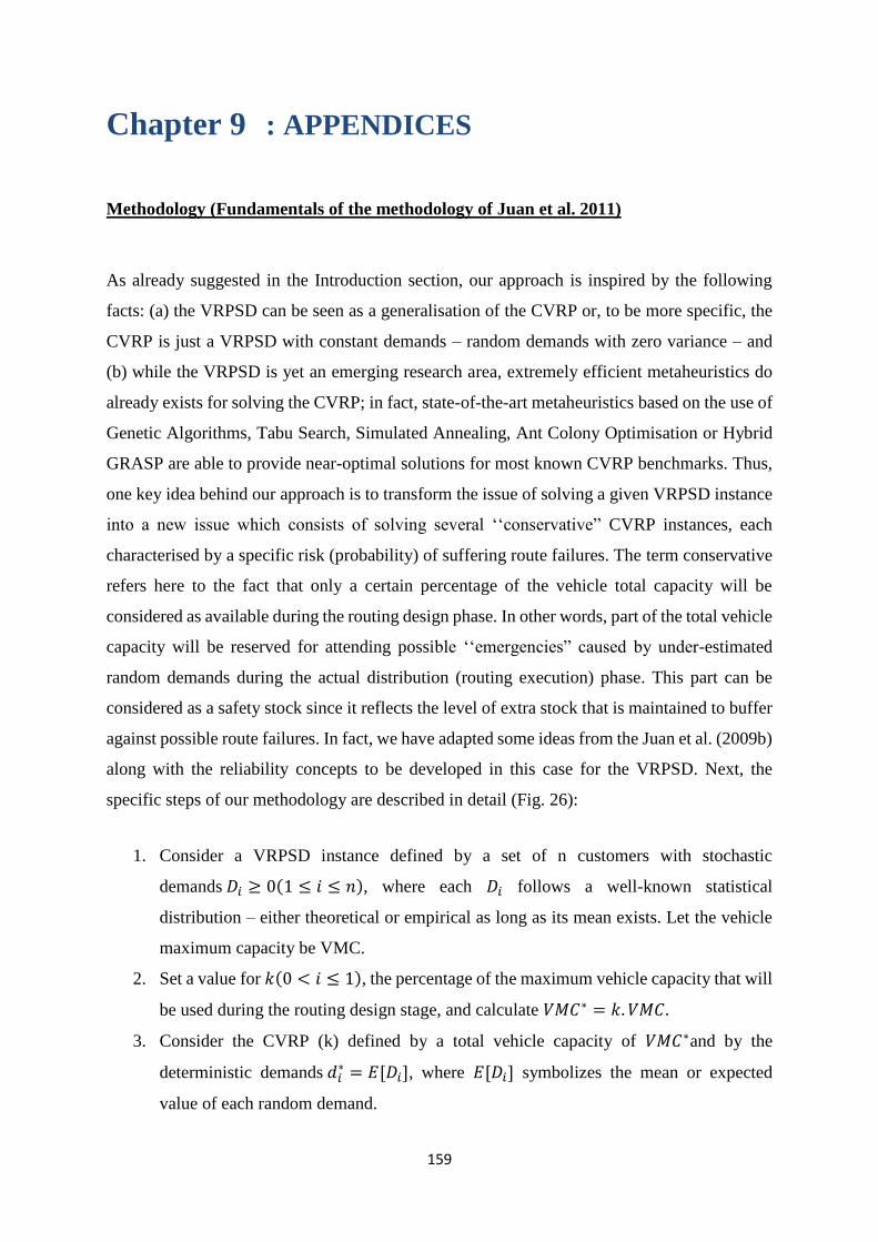
159

Chapter 9 : APPENDICES

Methodology (Fundamentals of the methodology of Juan et al. 2011)

As already suggested in the Introduction section, our approach is inspired by the following

facts: (a) the VRPSD can be seen as a generalisation of the CVRP or, to be more specific, the

CVRP is just a VRPSD with constant demands – random demands with zero variance – and

(b) while the VRPSD is yet an emerging research area, extremely efficient metaheuristics do

already exists for solving the CVRP; in fact, state-of-the-art metaheuristics based on the use of

Genetic Algorithms, Tabu Search, Simulated Annealing, Ant Colony Optimisation or Hybrid

GRASP are able to provide near-optimal solutions for most known CVRP benchmarks. Thus,

one key idea behind our approach is to transform the issue of solving a given VRPSD instance

into a new issue which consists of solving several ‘‘conservative” CVRP instances, each

characterised by a specific risk (probability) of suffering route failures. The term conservative

refers here to the fact that only a certain percentage of the vehicle total capacity will be

considered as available during the routing design phase. In other words, part of the total vehicle

capacity will be reserved for attending possible ‘‘emergencies” caused by under-estimated

random demands during the actual distribution (routing execution) phase. This part can be

considered as a safety stock since it reflects the level of extra stock that is maintained to buffer

against possible route failures. In fact, we have adapted some ideas from the Juan et al. (2009b)

along with the reliability concepts to be developed in this case for the VRPSD. Next, the

specific steps of our methodology are described in detail (Fig. 26):

1. Consider a VRPSD instance defined by a set of n customers with stochastic

demands 𝐷𝑖 ≥ 0(1 ≤ 𝑖 ≤ 𝑛), where each 𝐷𝑖 follows a well-known statistical

distribution – either theoretical or empirical as long as its mean exists. Let the vehicle

maximum capacity be VMC.

2. Set a value for 𝑘(0 < 𝑖 ≤ 1), the percentage of the maximum vehicle capacity that will

be used during the routing design stage, and calculate 𝑉𝑀𝐶∗ = 𝑘. 𝑉𝑀𝐶.

3. Consider the CVRP (k) defined by a total vehicle capacity of 𝑉𝑀𝐶∗and by the

deterministic demands 𝑑𝑖∗ = 𝐸 𝐷𝑖 , where 𝐸 𝐷𝑖 symbolizes the mean or expected

value of each random demand.

160

4. Solve the CVRP (k) by using any efficient CVRP methodology. Notice that the solution

of this CVRP is also an aprioristic solution for the original VRPSD. Moreover, it will

be a feasible VRPSD solution as long as there will be no route failure, i.e., as long as

the extra demand that might be originated during execution time in each route does not

exceed the vehicle reserve capacity (safety stock) 𝑉𝑅𝐶∗ = (1 − 𝑘). 𝑉𝑀𝐶. Notice also

that the cost given by this solution, 𝐶𝐶𝑉𝑅𝑃(𝑘), can be considered as a base or fixed cost

of the VRPSD solution, i.e., the cost of the VRPSD in case that no route failures occur.

Chances are that some route failures occur during the execution phase – these chances

increase as the value of 𝑘 gets closer to 1. If so, corrective actions – such as returning

to the depot for a reload before resuming distribution – and their corresponding variable

costs, 𝐶𝑅𝐹(𝑘), will need to be considered. Therefore, for a given value of k, the total

costs of the corresponding VRPSD solution will be the sum of the CVRP fixed costs

and the variable costs due to the corrective actions, i.e., 𝐶𝑉𝑅𝑃𝑆𝐷(𝑘) = 𝐶𝐶𝑉𝑅𝑃(𝑘) +

𝐶𝑅𝐹(𝑘). Notice that, on average, low values of k (close to 0) will be associated with

relatively high fixed costs (more routes will be needed to satisfy total demand) and

relatively low variable costs (route failure is less likely to occur). On the contrary, high

values of k (close to 1) will have the opposite effect.

5. Using the aprioristic solution with m routes, estimate the expected (average) costs due

to possible failures in the 𝑗𝑡ℎ route, 𝐸[𝐶𝑅𝐹𝑗 (𝑘)], ∀𝑗 = 1,2, … ,𝑚. This can be done by

using MCS, i.e., random demands are generated and whenever a route failure occurs

(or just before it happens), a corrective policy is applied and its associated costs are

registered (in the experimental section of this paper, every time a route fails we consider

the costs of a round-trip from the current customer to the depot; but, since we are using

simulation, other alternative policies and costs could also be considered in a natural

way). After iterating this process for some hundred/thousand times, a random sample

of observations regarding these variable costs are obtained and an estimate for its

expected value can be calculated. Then, the expected total costs due to possible route

failures in the aprioristic solution is given by the following expression: 𝐸 𝐶𝑅𝐹(𝑘) =

∑ 𝐸[𝐶𝑅𝐹𝑗 (𝑘)].𝑚

𝑗=1

6. Using the aprioristic solution with m routes, obtain an estimate for the reliability of

each route, 𝑅𝑗(1 ≤ 𝑗 ≤ 𝑚). In this context, 𝑅𝑗 is defined as the probability that the 𝑗𝑡ℎ

route will not suffer any failure during the distribution phase, i.e., that the 𝑗𝑡ℎ vehicle

will not run out of load before attending to all customer demands on its route. This

161

reliability value can be estimated by direct MCS using the statistical distributions that

model the customer demands in each route – observe that in each route over-estimated

demands could sometimes be compensated by under-estimated demands. To this end,

a number of trials – between several hundreds and several hundred thousand depending

of the desired accuracy – can be randomly generated. Each of these trials will provide

a random value for the total demand in a given route. Then, the relative frequency of

trials in which that total demand has not exceeded VMC can be used as an estimate of

the route’s reliability. Notice that 𝐹𝑗 = 1 − 𝑅𝑗 represents the probability that the 𝑗𝑡ℎ

route will fail during the distribution phase. Notice also that if the variances associated

with customer demands are not too large, it seems natural to expect no more than one

failure per route. Otherwise, more than a failure per route could occur.

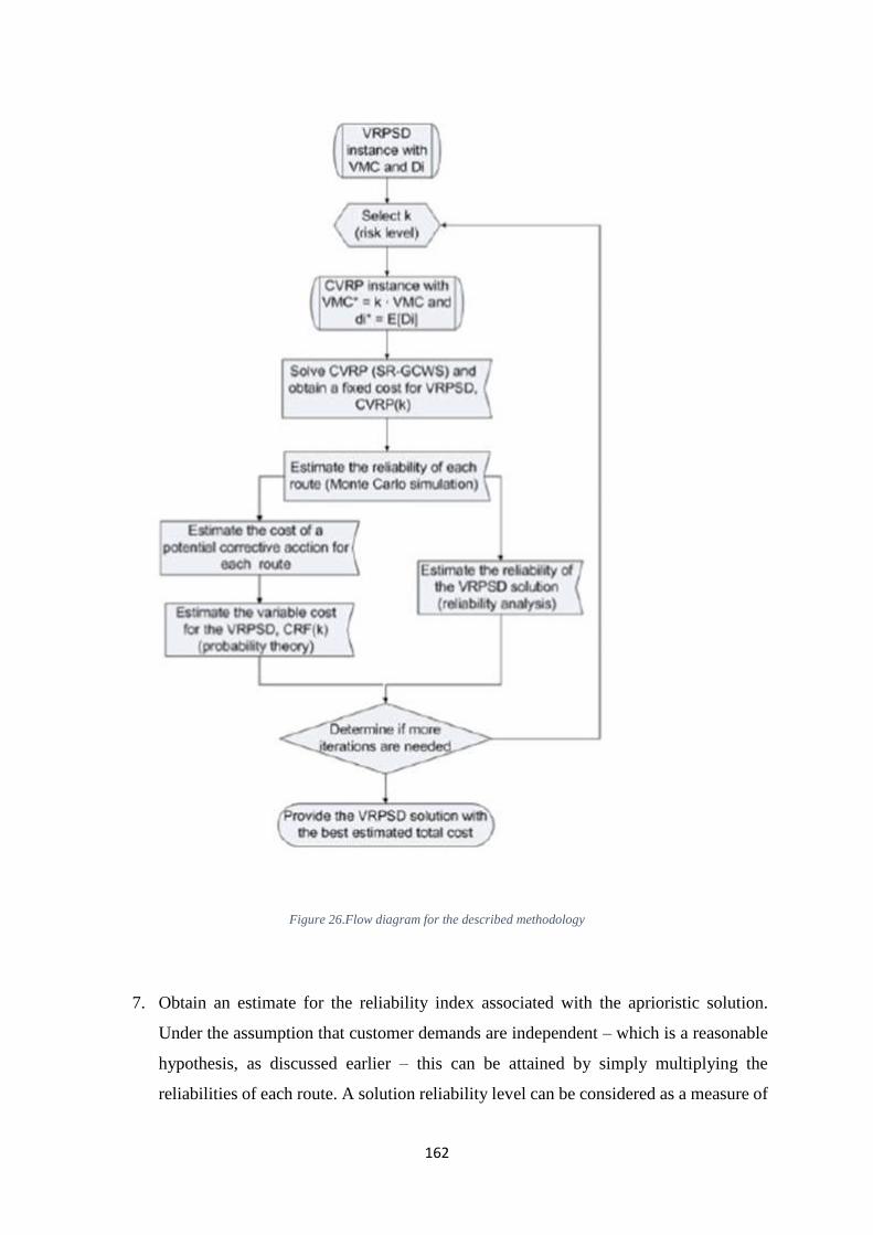
162

Figure 26.Flow diagram for the described methodology

7. Obtain an estimate for the reliability index associated with the aprioristic solution.

Under the assumption that customer demands are independent – which is a reasonable

hypothesis, as discussed earlier – this can be attained by simply multiplying the

reliabilities of each route. A solution reliability level can be considered as a measure of

163

the feasibility of that solution in the VRPSD context.

8. Depending on the total costs and the reliability indices associated with the solutions

already obtained, repeat the process from Step 1 with a new value of the parameter 𝑘–

i.e., explore different scenarios to check how different levels of safety stock affect the

expected total cost of the VRPSD solution.

9. Finally, provide a sorted list with the best VRPSD solutions found so far as well as their

corresponding properties (fixed costs, expected variable costs, expected total costs and

reliability index).

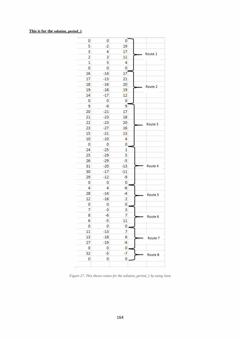
164

This is for the solution_period_1

.

Figure 27. This shows routes for the solution_period_1 by using Java

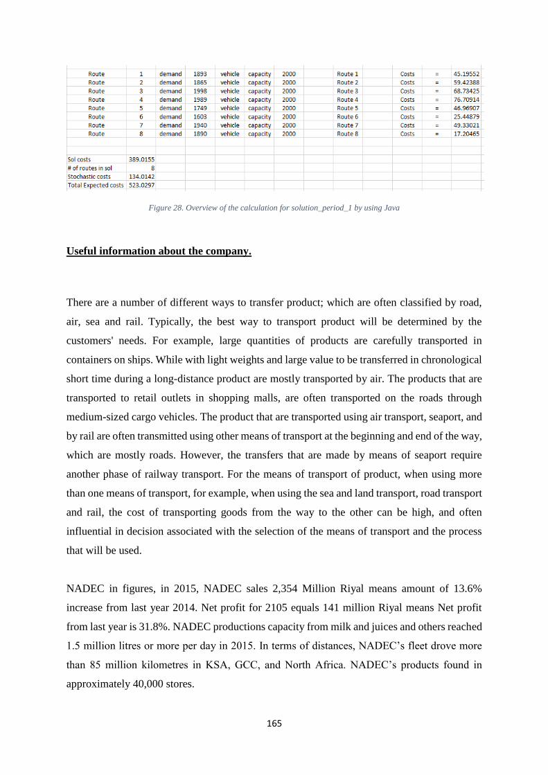
165

Figure 28. Overview of the calculation for solution_period_1 by using Java

Useful information about the company.

There are a number of different ways to transfer product; which are often classified by road,

air, sea and rail. Typically, the best way to transport product will be determined by the

customers' needs. For example, large quantities of products are carefully transported in

containers on ships. While with light weights and large value to be transferred in chronological

short time during a long-distance product are mostly transported by air. The products that are

transported to retail outlets in shopping malls, are often transported on the roads through

medium-sized cargo vehicles. The product that are transported using air transport, seaport, and

by rail are often transmitted using other means of transport at the beginning and end of the way,

which are mostly roads. However, the transfers that are made by means of seaport require

another phase of railway transport. For the means of transport of product, when using more

than one means of transport, for example, when using the sea and land transport, road transport

and rail, the cost of transporting goods from the way to the other can be high, and often

influential in decision associated with the selection of the means of transport and the process

that will be used.

NADEC in figures, in 2015, NADEC sales 2,354 Million Riyal means amount of 13.6%

increase from last year 2014. Net profit for 2105 equals 141 million Riyal means Net profit

from last year is 31.8%. NADEC productions capacity from milk and juices and others reached

1.5 million litres or more per day in 2015. In terms of distances, NADEC’s fleet drove more

than 85 million kilometres in KSA, GCC, and North Africa. NADEC’s products found in

approximately 40,000 stores.

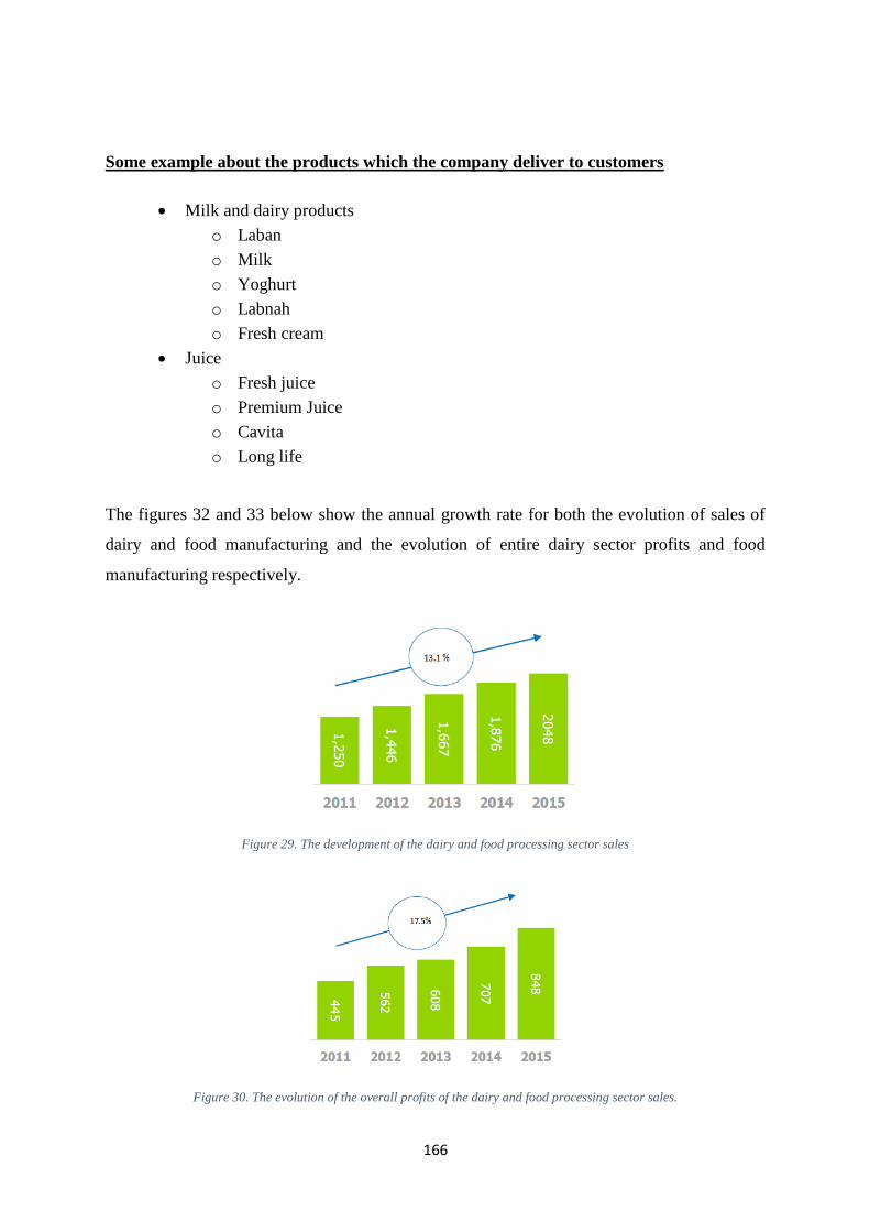
166

Some example about the products which the company deliver to customers

The figures 32 and 33 below show the annual growth rate for both the evolution of sales of

dairy and food manufacturing and the evolution of entire dairy sector profits and food

manufacturing respectively.

Figure 29. The development of the dairy and food processing sector sales

Figure 30. The evolution of the overall profits of the dairy and food processing sector sales.

Milk and dairy products

o Laban

o Milk

o Yoghurt

o Labnah

o Fresh cream

Juice

o Fresh juice

o Premium Juice

o Cavita

o Long life

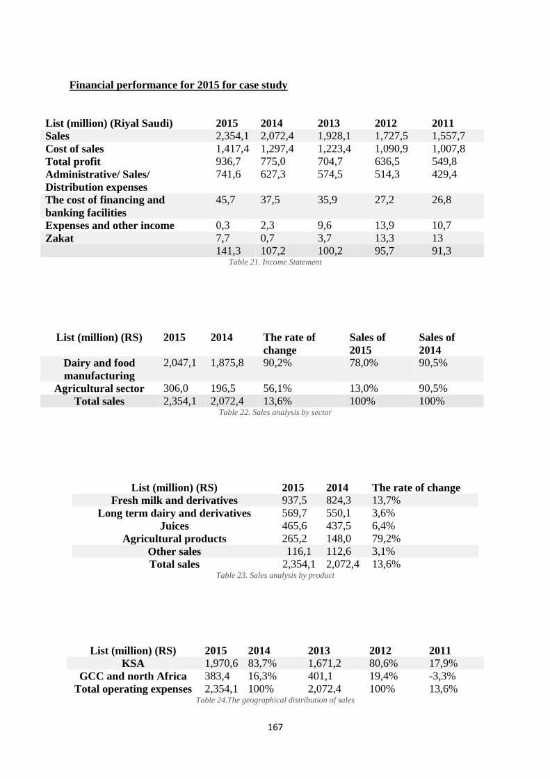
167

Financial performance for 2015 for case study

List (million) (Riyal Saudi) 2015 2014 2013 2012 2011

Sales 2,354,1 2,072,4 1,928,1 1,727,5 1,557,7

Cost of sales 1,417,4 1,297,4 1,223,4 1,090,9 1,007,8

Total profit 936,7 775,0 704,7 636,5 549,8

Administrative/ Sales/

Distribution expenses

741,6 627,3 574,5 514,3 429,4

The cost of financing and

banking facilities

45,7 37,5 35,9 27,2 26,8

Expenses and other income 0,3 2,3 9,6 13,9 10,7

Zakat 7,7 0,7 3,7 13,3 13

141,3 107,2 100,2 95,7 91,3 Table 21. Income Statement

List (million) (RS) 2015 2014 The rate of

change

Sales of

2015

Sales of

2014

Dairy and food

manufacturing

2,047,1 1,875,8 90,2% 78,0% 90,5%

Agricultural sector 306,0 196,5 56,1% 13,0% 90,5%

Total sales 2,354,1 2,072,4 13,6% 100% 100% Table 22. Sales analysis by sector

List (million) (RS) 2015 2014 The rate of change

Fresh milk and derivatives 937,5 824,3 13,7%

Long term dairy and derivatives 569,7 550,1 3,6%

Juices 465,6 437,5 6,4%

Agricultural products 265,2 148,0 79,2%

Other sales 116,1 112,6 3,1%

Total sales 2,354,1 2,072,4 13,6% Table 23. Sales analysis by product

List (million) (RS) 2015 2014 2013 2012 2011

KSA 1,970,6 83,7% 1,671,2 80,6% 17,9%

GCC and north Africa 383,4 16,3% 401,1 19,4% -3,3%

Total operating expenses 2,354,1 100% 2,072,4 100% 13,6% Table 24.The geographical distribution of sales

168

Dairy and food

processing sector

Agricultural

production sector

Total

2014-2015

List (million) (RS) 2015 2014 2015 2014 2015 2014

Sales 2,048 1,876 306 196 2,354 2,072

Total profit 847 707 90 68 937 775

All total 2,437 2,189 881 816 3,318 3,005 Table 25. Sectorial information