Road Condition Estimation Based on Heterogeneous Extended Floating Car Data

Kevin Laubis

FZI Research Center for Information

Technology, Germany laubis@fzi.de

Viliam Simko FZI Research Center

for Information Technology, Germany

simko@fzi.de

Alexander Schuller FZI Research Center

for Information Technology, Germany

schuller@fzi.de

Christof Weinhardt Karlsruhe Institute of Technology (KIT),

Germany weinhardt@kit.edu

Abstract

Road condition estimation based on Extended Floating Car Data (XFCD) from smart devices allows for determining given quality indicators like the international roughness index (IRI). Such approaches currently face the challenge to utilize measurements from heterogeneous sources. This paper investigates how a statistical learning based self-calibration overcomes individual sensor characteristics. We investigate how well the approach handles variations in the sensing frequency. Since the self-calibration approach requires the training of individual models for each participant, it is examined how a reduction of the amount of data sent to the backend system for training purposes affects the model performance. We show that reducing the amount of data by approximately 50 % does not reduce the models’ performance. Likewise, we observe that the approach can handle sensing frequencies up to 25 Hz without a performance reduction compared to the baseline scenario with 50 Hz. 1. Introduction

Modern cars equipped with GPS sensors and smart devices such as smartphones and mobile navigation systems carried in the vehicles allow for determining the position and speed of a car. The concept of collecting and analyzing streams of such position and speed data from multiple vehicles for determining traffic flows and directions in real time is called a Floating Car Data (FCD) approach. By estimating and predicting the overall traffic conditions based on FCD, road users can be assisted for instance by a rerouting to paths without congestions [1,2].

Besides the position and speed, other sensors can also be considered in the analysis, which leads to an Extended Floating Car Data (XFCD) approach. Thus,

a better insight into the traffic conditions and even the vehicles’ environment and the road surface is possible [3]. Estimating the road surface condition such as the longitudinal road roughness based on XFCD is beneficial for both, road users and road authorities.

Detailed and up-to-date insight into the road condition can benefit the drivers, especially in hazardous situations. Furthermore, avoiding rough road segments by rerouting to a smoother path and thus, lowering the vehicle wear, is an additional benefit [4].

Nowadays, road authorities conduct road condition measurements with the help of special purpose vehicles equipped with laser sensors that require trained personnel. Due to limited resources, the federal road network in Germany for example is monitored in four years intervals. This coarse granularity leads to a lack of information in the years between and thus, to inherently inefficient maintenance strategies, since road authority’s resource planning for performing maintenance actions like resurfacing or reconstruction of road segments have to rely on road deterioration models that are affected by uncertainty [5].

The XFCD approach proposed in this paper relies on measurements from a smartphone-equipped vehicle and is outlined in Figure 1. The overall goal is to leverage the potential of such vehicles for road condition estimation by allowing a seamless integration of new participants to the system. The main challenge is to handle the heterogeneity of the contributing cars and smart devices. Since the participants’ cars and devices can vary strongly (e.g. varying sensing frequencies), it is not possible to treat all sensor measurements with one single model. This requires fitting a unique model for each participant individually.

Since the (re-) training of unique models is computationally expensive and requires information about the road’s actual condition, it cannot be performed on the smart device itself, but has to be done in a backend system. For these training phases,

1582

Proceedings of the 50th Hawaii International Conference on System Sciences | 2017

URI: http://hdl.handle.net/10125/41344ISBN: 978-0-9981331-0-2CC-BY-NC-ND

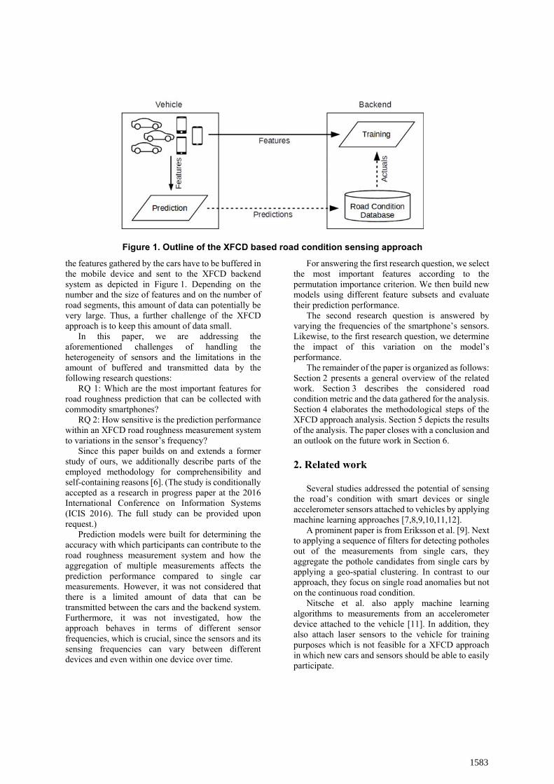
the features gathered by the cars have to be buffered in the mobile device and sent to the XFCD backend system as depicted in Figure 1. Depending on the number and the size of features and on the number of road segments, this amount of data can potentially be very large. Thus, a further challenge of the XFCD approach is to keep this amount of data small.

In this paper, we are addressing the aforementioned challenges of handling the heterogeneity of sensors and the limitations in the amount of buffered and transmitted data by the following research questions:

RQ 1: Which are the most important features for road roughness prediction that can be collected with commodity smartphones?

RQ 2: How sensitive is the prediction performance within an XFCD road roughness measurement system to variations in the sensor’s frequency?

Since this paper builds on and extends a former study of ours, we additionally describe parts of the employed methodology for comprehensibility and self-containing reasons [6]. (The study is conditionally accepted as a research in progress paper at the 2016 International Conference on Information Systems (ICIS 2016). The full study can be provided upon request.)

Prediction models were built for determining the accuracy with which participants can contribute to the road roughness measurement system and how the aggregation of multiple measurements affects the prediction performance compared to single car measurements. However, it was not considered that there is a limited amount of data that can be transmitted between the cars and the backend system. Furthermore, it was not investigated, how the approach behaves in terms of different sensor frequencies, which is crucial, since the sensors and its sensing frequencies can vary between different devices and even within one device over time.

For answering the first research question, we select the most important features according to the permutation importance criterion. We then build new models using different feature subsets and evaluate their prediction performance.

The second research question is answered by varying the frequencies of the smartphone’s sensors. Likewise, to the first research question, we determine the impact of this variation on the model’s performance.

The remainder of the paper is organized as follows: Section 2 presents a general overview of the related work. Section 3 describes the considered road condition metric and the data gathered for the analysis. Section 4 elaborates the methodological steps of the XFCD approach analysis. Section 5 depicts the results of the analysis. The paper closes with a conclusion and an outlook on the future work in Section 6.

2. Related work

Several studies addressed the potential of sensing

the road’s condition with smart devices or single accelerometer sensors attached to vehicles by applying machine learning approaches [7,8,9,10,11,12].

A prominent paper is from Eriksson et al. [9]. Next to applying a sequence of filters for detecting potholes out of the measurements from single cars, they aggregate the pothole candidates from single cars by applying a geo-spatial clustering. In contrast to our approach, they focus on single road anomalies but not on the continuous road condition.

Nitsche et al. also apply machine learning algorithms to measurements from an accelerometer device attached to the vehicle [11]. In addition, they also attach laser sensors to the vehicle for training purposes which is not feasible for a XFCD approach in which new cars and sensors should be able to easily participate.

Figure 1. Outline of the XFCD based road condition sensing approach

1583

In contrast to this paper, none of the known approaches investigate the model’s performance sensitivity to variations in the sensor’s frequency nor consider explicit feature selection mechanisms for data reduction reasons.

Feature selection methods for addressing the first research question can be divided into filter methods, wrapper methods and embedded methods [13].

Filter methods are performed as a preprocessing step before the actual model building and are mainly based on univariate or multivariate statistics, e.g. methods based on the mutual information criteria such as the minimum redundancy feature selection algorithm [14]. They are usually fast but do not make use of the learning model itself.

Wrapper methods make use of a certain learning algorithm by training models for different feature subsets and determining their relevance by comparing the prediction performances of models [15]. Even though, they perform best on the chosen algorithm if they are applied exhaustively, they are computationally expensive since the problem is exponential [16].

Embedded methods are inherently connected to a specific learning algorithm since the feature selection is performed within the training phase itself. Since they are making use of the learning algorithm without the need of building multiple models, we chose to apply the permutation importance for random forest as an embedded method for addressing the second research question of this paper [17].

3. Metric and data basis

The international roughness index (IRI) is a

commonly used metric for describing the condition of the longitudinal road’s profile. It is an indicator whether the road is rough and bumpy, whether it contains many pot holes or is in an overall wavy condition. It was announced by the World Bank in 1986 and is defined as the ratio of the accumulated suspension motion of a reference vehicle and the distance traveled [18]. The ratio can be given in the unit m/km. Although, it is defined by the suspension motion it is actually determined by measuring the road’s profile and then simulating the suspension system’s motion by a quarter-car-model [19]. Since the IRI is widely adopted and determined by most road authorities, it is the considered metric in this paper.

3.1. Ground truth

The Institute of Highway and Railroad

Engineering (ISE) at the Karlsruhe Institute of

Technology (KIT) provided us with a road’s actual profile measurements representing a distance of 2.28 km on the district road K3535 in Baden-Württemberg, Germany in both directions. This profile was measured by special laser-equipped vehicles. We calculate the IRI for 100 m segments with an overlap of 80 m. This results in overall 220 samples for 4.56 km. These values are used as ground truth for the model training. The considered IRI values range from 0.8 m/km to 2.94 m/km. The median is 1.2 m/km and the variance is 0.147.

3.2. Test drives

For generating XFCD for the analysis, we perform

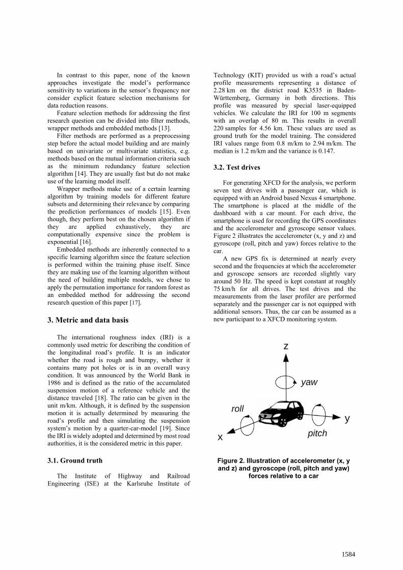
seven test drives with a passenger car, which is equipped with an Android based Nexus 4 smartphone. The smartphone is placed at the middle of the dashboard with a car mount. For each drive, the smartphone is used for recording the GPS coordinates and the accelerometer and gyroscope sensor values. Figure 2 illustrates the accelerometer (x, y and z) and gyroscope (roll, pitch and yaw) forces relative to the car.

A new GPS fix is determined at nearly every second and the frequencies at which the accelerometer and gyroscope sensors are recorded slightly vary around 50 Hz. The speed is kept constant at roughly 75 km/h for all drives. The test drives and the measurements from the laser profiler are performed separately and the passenger car is not equipped with additional sensors. Thus, the car can be assumed as a new participant to a XFCD monitoring system.

Figure 2. Illustration of accelerometer (x, y and z) and gyroscope (roll, pitch and yaw)

forces relative to a car

1584

4. Methodology

The following steps with the objective of determining the features’ importance and for investigating the models’ sensitivity to variations in the sensors frequency are performed for each of the seven drives.

4.1. Map-matching

As a first step, we start with GPS fixes represented

as a set . Every GPS fix ∈ is a tuple: , , (1)

, are GPS coordinates – latitude and longitude WGS-84 (e.g. 56.78901)

is a UTC timestamp (in milliseconds). For convenience, we use the notation to denote the timestamp of a particular GPS fix .

We use a map-matching algorithm , which uses the road network information :

↦ ′ (2) ′ is a new set of GPS coordinates that are matched

to the actual road network . Both sets are of the same size, i.e, ∥ ∥ ∥ ∥.

This map-matching to a road network, common to all seven drives and to the laser measured IRI, is used to align measurements from multiple cars and the actual road conditions. The OpenStreetMap is used as the common road network . We apply a hidden Markov model based map-matching that considers inverse distance weighting between GPS fixes and the road positions [20]. The map-matching approach makes use of the Viterbi algorithm for maximizing the product of measurement probabilities and transition probabilities to determine the most likely route. An open source map-matching implementation from the project Open Street Routing Machine (OSRM) is used in this study [21]. Timestamps did not change during map-matching, i.e.,

∀ : ∈ , ∈ , , , ,, ,

(3)

For defining common slots on the road network, the determined road link is subdivided equidistantly every 10 . This distance is chosen to be able to consider frequencies up to 200 Hz without information loss, assuming a speed of at least 72 km/h.

We use a function that converts matched GPS fixes into virtual GPS fixes that are equidistantly placed on the road (with distance ). The size of is much larger than , i.e., ∥ ∥≫ ∥ ′ ∥.

, ↦ , (4)

∀ ∈ : ∀ ∈ , :

∥ ∥. ∥ ′ ∥

Function ′ finds the next matched GPS coordinate based on timestamp from ′.

Function , returns all virtual GPS fixes ∈ such that it holds:

(5)

4.2. Feature extraction The sensor readings are assigned to the virtual

GPS fixes . If multiple readings are assigned to one GPS fix, they are aggregated by their mean. A continuous linear approximation is also applied to the sensor data :

↦ ′ (6) Thus, the virtual GPS fixes and the approximated

sensor data can be assigned by their timestamps:

, ′ ↦ ∈ ′: ∃ ∈ ,

(7)

Note: After this data alignment step, the data is equidistantly sampled in space. This allows for aggregation of different sources and eases the further analyses.

The data set can be assumed as a matrix with rows and columns. Columns represent features , … , . Rows represent samples , … , . Each

sample belongs to a slot of length 10  . Each sample with index 1,… , is defined as follows:

, … , (8) The matrix is then defined as follows:

⋮…

⋮ ⋱ ⋮…

(9)

We also define a function which assigns a natural number (context size) for each feature , i.e.,

↦ (10) This number represents how many neighboring

samples contribute to the computation of a single sample. The context size for the whole matrix is as follows:

max…

(11) Note: The last feature represents the outcome

variable. Next to the accelerometer and gyroscope readings,

the GPS speed is considered as an additional feature source. From the accelerometer sensor we consider the absolute readings as well as the relative linear acceleration excluding the gravity. The raw data stream from each sensor is aggregated per 100 m segments. The reason for choosing 100 m segments is because most of official road condition monitoring

1585

systems also consider this segment size. This aggregation of 100 m segments is performed in a continuous manner for every 10 cm slot. We consider the aggregation functions mean, range, standard deviation, variance and root mean square since they are also considered in the related work.

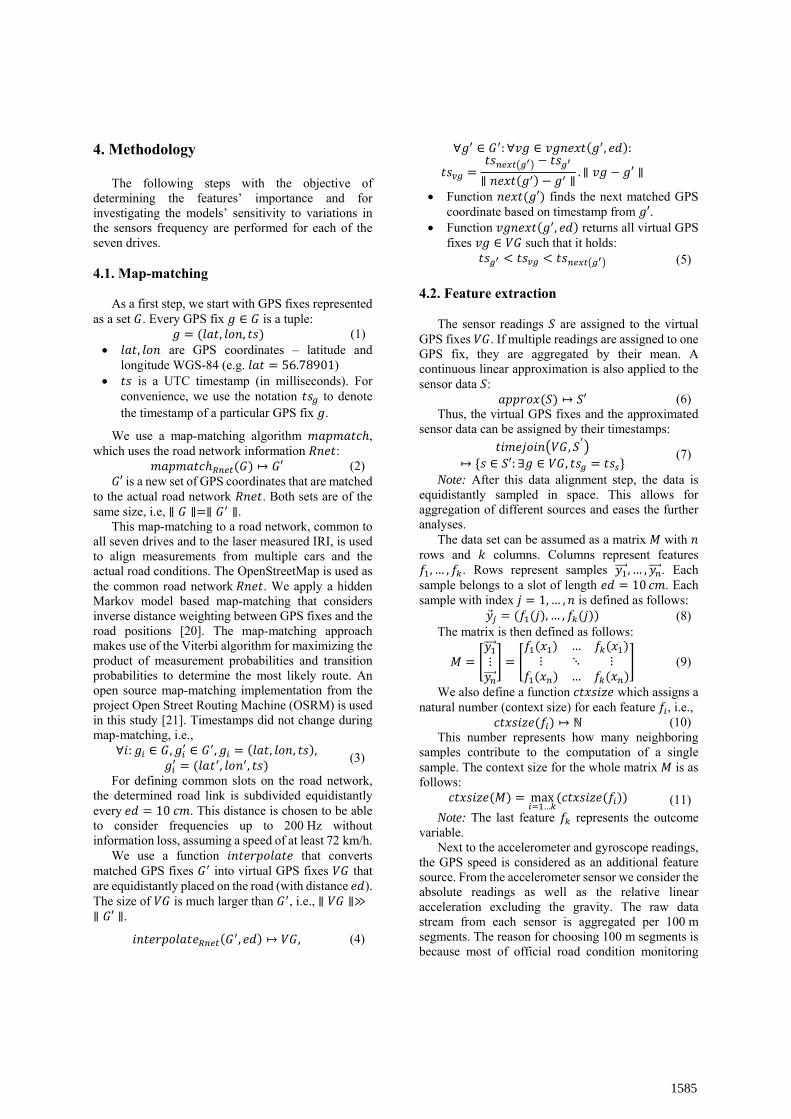
Since the road’s waviness could be described by frequencies, we also perform a continuous wavelet transformation (CWT) to the accelerometer and gyroscope readings for extracting features reflecting the frequency content [22]. Hereby, features with a contextual information of 0.4 m (hh), 0.8 m (h), 2.26 m (m), 9.05 m (l) and 51.21 m (ll) are chosen. Even though, most likely the features with a smaller contextual information are important, we also extracted the larger ones for determining their importance. Table 1 summarizes the resulting 95 features, which are all z-score normalized.

4.3. Model building

A random forest regression model is built for every

drive separately with the actual IRI as the outcome variable [17]. We chose random forests since in our former study they outperform other methods such as support vector machines [23]. This could be because random forests can handle problems with a small number of observations and a high number of predictors very well without overfitting. Furthermore, due to the random selection of features per tree, random forests can also cope with multicollinearity.

With respect to the overlapping 100 m road segments for which we have the actual IRI values, we chose every corresponding 200th sample from the data set derived from the test drives. Likewise, this results in 220 samples per drive. This overall set is split into 80 % training data and 20 % test data. Hereby it is taken care of not spilling the information from overlapping samples to the test set. In addition to this overall data splitting, each model was time slicing cross validated and tuned by the number of randomly chosen features for each tree for addressing the overfitting. The metric considered for cross validation is the coefficient of determination R².

4.4. Feature importance

For reducing the amount of data that has to be

stored on the smartphone and that has to be sent to the backend system for model training purposes, the most important features are determined by computing the permutation importance [17]. The permutation importance is a method for feature importance determination that is embedded in the random forest training algorithm. Thus, it considers the model’s

performance directly and can be efficiently determined within a single training phase. Therefore, the permutation importance is deployed in this paper instead of filter or wrapper methods, which either do not make use of the model specific information or require multiple training phases with different feature subsets.

The permutation importance for the feature within tree with ∈ 1,… , is defined as

follows:

∑ ∈

| |

∑ ,∈

| |

(12)

Where is the out-of-bag sample for tree and determines the out-of-bag performance based on the

actual and predicted values, e.g. the mean squared error (MSE). is the prediction of observation . , is the prediction of

observation where the value of the feature was permuted. That means the following:

, … , , , … ,(13)

The overall permutation importance for between all trees is determined by the mean permutation importance over all trees :

∑ (14)

Thus, for every feature the mean performance decrease is determined as the difference between the performance with and without permuting the feature’s value.

Table 1. Features extracted from smartphone’s sensors

Sensor Aggregation Function

Number of Features

GPS speed mean, range, sd, var., rms

5

Accelerometer (3-axis)

mean, range, sd, var., rms, CWT for 5 bands

30

Linear accelerometer (3-axis)

mean, range, sd, var., rms, CWT for 5 bands

30

Gyroscope (3-axis)

mean, range, sd, var., rms, CWT for 5 bands

30

1586

For features that are unimportant because they do not have a relation to the outcome or because there is multicollinearity in the feature set, the permutation does not result in a large performance difference. However, for features that are important, the performance should decrease if the values of that feature are permuted.

4.5. Sensor frequency

Since it cannot be assured that all smart devices

contribute with the same frequencies and since an individual feature extraction and model building is performed to allow contributions from a heterogeneous set of smart devices, we investigated the effect of variations in the sensing frequency on the XFCD approach. Even though, the same Nexus 4 smartphone is used for all test drives, a variation in the sensor’s frequency is achieved by subsampling the gathered data. Thus, it is possible to determine whether the findings hold for sensor types and smartphones with other sensing frequencies as well.

The subsampling is done by reducing the number of readings in the sensor data according to different sampling rates. Thought, that the maximum frequency is the actual one with approximately 50 Hz, we additionally considered frequencies of 25 Hz, 15 Hz and 5 Hz. The upper bound is chosen since 25 Hz approximately relates to the empirically determined Android sensor delay type or sampling rate “UI” of the considered Nexus 4. The lowest chosen frequency relates to the Android sensor delay type “Normal”.

For each new subsample, the continuous approximation (Equation 6), the joining with the virtual GPS fixes (Equation 7), the generation of the feature matrix (Equation 9) and the model training and testing (Equations 14 and 15) is performed again.

5. Results

The single prediction models are tested on the remaining out of sample test set. The performance of each model is given by its coefficient of determination R² and is presented in Table 2. The R² indicates how much of the variance in the ground truth data is explained by the prediction model. It is a widely used metric for determining the goodness of fit of a model and since it is a relative measure, it is easy to interpret and more easily comparable among models than e.g. absolute error metrics.

It is shown that single cars can contribute to a XFCD based road roughness measurement system with a mean R² of 67.83 %. For the considered seven drives the R² ranges from 59.68 % to 76.79 %. These

performances are considered as the baseline for the feature selection analysis and for the sensitivity analysis in terms of the sensing frequencies.

5.1. Feature selection

For answering the first research question, the most

important features for road roughness prediction that can be collected with commodity smartphones are determined by computing the permutation importance for each feature and ranking them accordingly. Figure 3 shows the mean permutation importance over all seven drives for the ten most important features.

The features extracted from the x-axis gyroscope are prevalent in the ten most important features. Thus, the information whether the vehicle is rolling does have a high explanatory value for estimating the IRI. Next to these features, the y-axis gyroscope (pitch) is also important for the estimation since three of its features are present among the top ten. For both, roll and pitch, the variance seems to be the best aggregation function. The CWT features with the two lowest frequency bands extracted from the x-axis gyroscope appear in the top ten. Thus, for the roll behavior of the vehicle, the bands with a contextual information of 9.05 m and 51.21 m are more important than those with a smaller contextual information. From the accelerometer sensor just the variance of the x-axis is one of the ten most important features.

Figure 4 indicates the mean permutation importance for the ten least important features. It is shown that seven out of these ten features are extracted from acceleration sensors. Four out of these features are extracted from the absolute and linear y-axes acceleration. Although, the pitch and roll sensors are

Table 2. Out of sample performance of single models

Drive R²

1st Drive 0.6319

2nd Drive 0.5968

3rd Drive 0.6207

4th Drive 0.7395

5th Drive 0.7679

6th Drive 0.7115

7th Drive 0.6799

Max 0.7679

Mean 0.6783

Min 0.5968

1587

dominant in the ten most important feature set, the mean aggregation function of both sensor values is unimportant for the prediction. This indicates that the variation in the sensor’s measurements is more important than the absolute value.

A sensitivity analysis is performed for evaluating the effect of the permutation important based feature selection on the models’ performance. The baseline is the models’ performance, which considered the full set of 1 features. Compared to this baseline we determine the performances for models with the

, , , and most important features.

The result of this comparison is given in Figure 5. It is shown, that reducing the number of features from 95 to 48 – which is a data size reduction of nearly 50 % – does not lead to a decrease in the median R² over all drives. Further reducing the number of features leads to a performance decrease. However, only considering twelve features still allows for an out of sample R² of more than 50 % for each model trained. Reducing the number of considered features to six or less leads to a performance reduction to an R² of 21 % and less for single models.

5.2. Sensitivity to sensing frequency

For answering the second research question, how

sensitive the prediction performance within an XFCD road roughness measurement system is to variations in the sensor’s frequency, the results of the sensitivity analysis addressing the variation in the sensing frequencies are given in Figure 6. The 50 Hz boxplot serves as the baseline and is equal to the corresponding boxplot in Figure 5 (95 features boxplot).

Reducing the sensor’s frequency to 25 Hz causes a minor increase in the median performance. However, the first and third quartiles are both lower than those from the 50 Hz boxplot. Furthermore, the performances of the single models are more spread and thus, the predictions are not as reliable as those from the baseline models. A further reduction of the sensor’s frequency to 15 Hz leads to a reduction of the median performance from an R² of 0.6923 to 0.6319. Considering a frequency of 5 Hz further reduces the performance to an R² of 0.6205.

Figure 3. Mean permutation importance of ten most important features

Figure 4. Mean permutation importance of ten least important features

1588

Next to the moderate performance decrease it has to be mentioned, that for the frequency of 5 Hz there is a single model with a low performance with an R² of 0.4031.

6. Conclusion and outlook

In this paper, an XFCD approach for estimating the longitudinal road roughness by smartphone equipped passenger cars is evaluated. The considered metric for the longitudinal road condition is the IRI.

Seven test drives are performed for collecting accelerometer and gyroscope measurements. Features are extracted from these measurements and aligned with the laser-measured road’s actual IRI values. For every test drive, a random forest regression model is built and tuned for estimating the road’s IRI values. Since different sampling distances and road segment lengths are considered in this paper, we summarize these for clarification. The ground truth IRI values are provided for overlapping 100 m road segments with a 20 m offset. The relevant road link is split in equidistant slots with a distance of 10 cm. The sensor measurements are aligned to these slots by map-matching and interpolation. For extracting features continuously, each slot is considered as one sample. For the model training and testing a subset of this resulting set of samples is chosen in a way that there is one sample kept for each corresponding ground truth IRI value.

The single prediction models have an out of sample R² of 0.6783 on average. Thus, they explain 67.83 % of the ground truth’s variance. The performance ranges from an R² of 0.5968 at minimum to 0.7679 at maximum. These model performances are considered as a baseline to answer the two research questions.

The permutation importance was determined for all features over all test drives. It is shown that features extracted from the x-axis gyroscope readings are very important and the y-axis accelerometer readings are less important for the prediction models. Reducing the feature set by keeping the 50 % more important features (from 95 features to 48 features) does not lead to a reduction in the median performance of the models. However, further reducing the feature set leads to a drop in the median R².

Analyzing the model’s sensitivity to different sensing frequencies shows that a reduction from 50 Hz to 25 Hz does not cause a reduction in the median out of sample R². Even though, these measurements have a higher variance, an integration of multiple predictions could eliminate this uncertainty of single models. Thus, it is shown that variations in the sensing frequency can be handled by the XFCD approach.

Future work has to address the managerial implications of a service based on this XFCD approach. It has to be investigated which model performance is required for substituting or supplementing the current laser-based road condition

Figure 6. Sensitivity of prediction performance to sensor frequency

Figure 5. Sensitivity of prediction performance to number of features

1589

monitoring. Hereby two main stakeholders have to be considered – road users and road authorities.

Road users can benefit from a nearly real time road condition monitoring by being warned about hazardous situations and by adopting their driving behavior to the current road condition. Thus, they e.g. can avoid costs caused by accidents and reduce the vehicle’s wear by avoiding roads that are in a bad condition.

Since the IRI is an important predictor for the overall road’s condition, it is used for calculating optimal road maintenance strategies [5]. Thus, it e.g. can be determined when a road should be resurfaced or reconstructed. Due to the coarse granularity of current road monitoring intervals, the strategies have to rely on road deterioration models. Future work should address how accurate road condition measurements need to be to be meaningful for determining beneficial road maintenance strategies.

Knowing the required model performance from both, road users and road authorities, on the one hand it can be determined what amount of considered features are required to be sent to the backend system and on the other hand the minimum sensing frequency of the smartphone-equipped cars can be identified.

7. Acknowledgement

The Institute of Highway and Railroad Engineering (ISE) at the Karlsruhe Institute of Technology provided data about the actual road’s profile, which was considered as ground truth within this study.

8. References

[1] X. Kong, Z. Xu, G. Shen, J. Wang, Q. Yang, and B. Zhang, “Urban traffic congestion estimation and prediction based on floating car trajectory data”, Future Generation Computer Systems 61(1), 2016, pp. 97-107.

[2] C. de Fabritiis, R. Ragona, and G. Valenti, “Traffic Estimation And Prediction Based On Real Time Floating Car Data”, in 2008 11th International IEEE Conference on Intelligent Transportation Systems, IEEE, Beijing, 2008, pp. 197-203.

[3] D. Irschik, and W. Stork, “Road surface classification for extended floating car data”, in 2014 IEEE International Conference on Vehicular Electronics and Safety, IEEE, Hyderabad, 2014, pp. 78-83.

[4] K. Laubis, V. Simko, and A. Schuller, “Crowd Sensing of Road Conditions and its Monetary Implications on Vehicle Navigation”, in Proceedings of the 2nd IEEE

International Conference on Internet of People, IEEE, Toulouse, 2016, pp. 833-840.

[5] Y. Ouyang, and S. Madanat, „Optimal scheduling of rehabilitation activities for multiple pavement facilities: exact and approximate solutions“, Transportation Research Part A: Policy and Practice 38(5), 2004, pp. 347-365.

[6] K. Laubis, V. Simko, and A. Schuller, “Road Condition Measurement and Assessment: A Crowd Based Sensing Approach”, FZI Research Center for Information Technology, Karlsruhe, Rep., 2016.

[7] R. Bhoraskar, N. Vankadhara, B. Raman, and P. Kulkarni, “Wolverine: Traffic and road condition estimation using smartphone sensors”, in Proceedings of the 4th International Conference on Communication Systems and Networks, Bangalore, 2012, pp. 1-6.

[8] Y. Du, C. Liu, D. Wu, and S. Jiang, “Measurement of International Roughness Index by using Z-Axis Accelerometers and GPS”, Mathematical Problems in Engineering, 2014, pp. 1-10.

[9] J. Eriksson, L. Girod, B. Hull, R. Newton, S. Madden, and H. Balakrishnan, “The Pothole Patrol: Using a Mobile Sensor Network for Road Surface Monitoring”, in Proceeding of the 6th International Conference on Mobile Systems, Applications, and Services – MobiSys ’08, Breckenridge, 2008, pp. 29-39.

[10] P. Mohan, V. N. Padmanabhan, and R. Ramjee, “TrafficSense: Rich Monitoring of Road and Traffic Conditions using Mobile Smartphones”, in Proceeding of the 6th ACM Conference on Embedded Network Sensor Systems, Raleigh, 2008, pp. 1-29.

[11] P. Nitsche, C. Van Geem, R. Stütz, I. Mocanu, and L. Sjögren, “Monitoring ride quality on roads with existing sensors in passenger cars”, in Proceedings of the 26th ARRB Conference, Sydney, 2014, pp. 1-13.

[12] M. Perttunen, O. Mazhelis, F. Cong, M. Kauppila, T. Leppänen, J. Kantola, J., Collin, S. Pirttikangas, J. Haverinen, T. Ristaniemi, and J. Riekki, Distributed Road Surface Condition Monitoring Using Mobile Phones. Ubiquitous Intelligence and Computing, Berlin, Springer, 2011, pp. 64-78.

[13] I. Guyon, and A. Elisseeff, „An Introduction to Variable and Feature Selection“, Journal of Machine Learning Research 703(3), 2003, pp. 1157-1182.

[14] B. Auffarth, M. Lopez, and J. Cerquides, Comparison of redundancy and relevance measures for feature selection in tissue classification of CT images. Advances in Data Mining, Berlin, Springer, 2010, pp. 248-262.

1590

[15] R. Kohavi, and G. H. John, „Wrappers for feature subset selection“, Artificial Intelligence 97(1-2), 1997, pp. 273-324.

[16] E. Amaldi, and V. Kann, „On the approximability of minimizing nonzero variables or unsatisfied relations in linear systems“, Theoretical Computer Science 209(1), 1998, pp. 237-260.

[17] L. Breiman, “Random Forests”, Machine Learning 45(1), 2001, pp. 5-32.

[18] M. W. Sayers, T. D. Gillespie, and C. A. V. Queiroz, The International Road Roughness Experiment – Establishing Correlation and a Calibration Standard for Measurements. The World Bank Technical Paper, Washington, D.C., Transportation Department, 1986.

[19] R. N. Jazar, Vehicle Dynamics: Theory and Application, New York, Springer, 2014.

[20] P. Newson, and J. Krumm, "Hidden Markov map matching through noise and sparseness", in Proceedings of the 17th ACM SIGSPATIAL International Conference on Advances in Geographic Information Systems, Seattle, 2009, pp. 336-343.

[21] D. Luxen, and C. Vetter, “Real-time routing with OpenStreetMap data”, in Proceedings of the 19th ACM SIGSPATIAL International Conference on Advances in Geographic Information Systems – GIS ’11, Chicago, 2011, pp. 513-516.

[22] C. Torrence, and G.P. Compo, “A practical guide to wavelet analysis”, Bulletin of the American Meteorological Society 79(1), 1998, pp. 61-78.

[23] B. Schölkopf, and J. S. Alexander, Learning with Kernels: Support Vector Machines, Regularization, Optimization, and Beyond, Cambridge, MIT Press, 2002.

1591