Structural Estimation and Solution of InternationalTrade Models with Heterogeneous Firms

Edward J. Balistreri∗

Colorado School of Mines

Russell H. HillberryUniversity of Melbourne

Thomas F. RutherfordAnn Arbor, MI

October 2007

Abstract

We present an empirical implementation of a general-equilibrium model of interna-tional trade with heterogeneous manufacturing firms. The theory underlying our modelis consistent with Melitz (2003). A nonlinear structural estimation procedure identifiesa set of core parameters and unobserved firm-level trade frictions which best fit thegeographic pattern of trade. Once the parameters are identified, we utilize a decom-position technique for computing general-equilibrium counterfactuals. We illustratethis technique using trade and protection data from the Global Trade Analysis Project(GTAP). We first assess the economic effects of reductions in measured tariffs. Takingthe simple-average welfare change across regions the Melitz structure indicates wel-fare gains from liberalization that are nearly four times larger than in a standard pol-icy simulation model. Furthermore, when we compare the economic impact of tariffswith reductions in estimated fixed trade costs we find that policy measures affecting thefixed costs of firm entry are of greater importance than conventional tariff barriers. (JELC68,F12)

∗Corresponding author: Engineering Hall 311, Division of Economics and Business, Colorado School ofMines, Golden, CO 80401-1887; email: ebalistr@mines.edu.

1 Introduction

In canonical models of international trade, trade policy changes induce factors of produc-

tion to move between industries. Recent empirical and theoretical developments suggest

that within-industry factor movements may also be an important channel through which

policy affects economic variables. Studies of plant level data document significant intra-

industry differences in productivity levels.1 The movement of factors from less-productive

to more-productive plants is an important channel of productivity growth.2 An empirical

literature has begun linking trade to productivity growth via these channels.3

A recent theoretical model by Melitz (2003) rationalizes these and other empirical phe-

nomena within a general equilibrium model of production and trade. A fixed entry cost and

differentiated products allow equilibrium co-existence of firms with heterogeneous produc-

tivities. Fixed costs of trade ensure that only more productive firms export. Among these,

a smaller subset of even more productive firms serve multiple export markets. Trade liber-

alization raises industry productivity by shifting market share away from low-productivity

non-exporters, and toward high-productivity exporters. Trade liberalization also improves

welfare by increasing the number of imported varieties available to domestic consumers.

These qualitative features of the model are important. Our purpose is to apply the theo-

retic innovations to a quantitative analysis of policy. The model relies upon parameters that

are difficult to measure directly. Fixed costs of trade play an important role in this frame-

work, but they are typically unobserved. Another of the model’s key parameters, the implicit

shape of the productivity distribution, is not observed directly. Even indirect estimates of

this parameter rely on confidential access to plant-level data.

Recent papers in the geography-of-trade literature use structural assumptions and the

1Bartelsman and Doms (2000) review this literature.2See Foster et al. (2001), among others.3Pavcnik (2002)

1

bilateral pattern of trade to make inferences about the size of trade costs. Anderson and

van Wincoop (2003) develop a structural estimation technique that can be used to infer

trade costs. Balistreri and Hillberry (2007) develop an alternative estimation strategy for the

same model, and argue that it can be extended to most general equilibrium models of trade.

Balistreri and Hillberry (forthcoming) link structural estimation techniques to established

methods for calibrating general equilibrium models. We adapt these methods to calibrate

a multi-sector, multi-region general equilibrium model in which the manufacturing sector

has a Melitz-style market structure.

A key technical challenge in the development of this method is an algorithm for efficient

solution of a multi-dimensional model with heterogeneity in plant level productivity. This is

computationally difficult because the model requires joint solution of the trade equilibrium

and a host of entry conditions identifying marginal firms. To solve this problem, we decom-

pose the general equilibrium into an industry-specific module which determines the indus-

trial organization and a general equilibrium model which evaluates relative prices, compar-

ative advantage and the terms of trade. The full general equilibrium solution is achieved

through an iterative procedure in which the exchange equilibrium is solved conditional on

the industrial organization.

Our structural estimation procedure uses the equations defined by the numeric model

as a series of side constraints on the econometric objective. The model is underidentified,

but assumptions about a few key structural parameters allow the econometric procedure to

complete the identification of both the production technology and average bilateral trade

costs. Leaning heavily on our structural model, we attribute differences between observed

and fitted bilateral trade in manufactured goods to unobserved fixed costs of trade. This

interpretation allows us to generate a complete, exact calibration of the model, without any

role for idiosyncratic preferences in manufacturing trade.

The key structural parameters of the model are the distance elasticity of ad valorem trade

2

costs and the parameter defining the shape of the Pareto distribution of firm level productiv-

ities. We estimate these under three different sets of identifying assumptions. Our preferred

specification ties down the distance elasticity of trade costs, using unexplained variation in

the trade pattern to fit the implied shape of the productivity distribution. Our estimate of

this parameter is largely consistent with estimates from the confidential plant-level data.

With our general equilibrium system fully parameterized, we proceed to a quantitative

assessment of the effect of trade policy changes. Using a standard Armington structure as

the benchmark, we consider a 50 percent reduction in manufacturing tariffs. As expected,

endogenous productivity changes and growth in the number of imported varieties lead to

larger welfare changes in the Melitz model than in the Armington baseline. Taking the simple-

average welfare change across regions, the Melitz structure indicates welfare gains from lib-

eralization that are nearly four times larger than those from the baseline model. We also

consider reductions in the inferred bilateral fixed costs, and find that the welfare gains from

these changes are substantially larger. Joint reductions of tariffs and the inferred fixed costs

of trade generate even larger welfare gains. When we reduce both tariffs and fixed border

costs by 50% the average welfare gain is nearly 30 times larger than in the case of tariff cuts

in the Armington structure.

In section 2 we provide a review of the relevant literature, with a focus on the empiri-

cal literatures on heterogeneous productivity and the geographic pattern of trade. Section

3 provides a brief review of the Melitz (2003) theory as it relates to our application. Sec-

tion 4 details a practical method for numerically solving the heterogeneous-firms model. In

Section 5 we outline the nonlinear estimation procedure, and estimate the structural pa-

rameters that allow the model to best fit the data. These parameters are used to calibrate an

operational general equilibrium model, which we employ to conduct counterfactual analy-

sis. The results of this analysis appear in section 6. In section 7 we discuss implications of

our work and directions for further research.

3

2 Literature Review

Two broad areas of the empirical trade literature motivate the models like those proposed in

Melitz (2003) or Bernard et al. (2007).

First, an extensive literature has documented heterogeneity across establishments in

productivity, export behavior and responses to trade shocks. Important findings from this

literature include a) there is wide variation in productivity levels among coexisting plants;4 b)

only a small fraction of establishments engage in exporting, and exporters tend to be larger

and more productive than non-exporters;5 c) there is considerable heterogeneity among ex-

porters in the number of markets served per firm;6 d) within-industry reallocation of market

share from less-productive to more-productive establishments is an important component

of aggregate productivity growth;7 and e) productivity growth via shifting market shares (in-

cluding the exit of the lowest productivity plants) is an important channel through which

trade cost reductions induce aggregate productivity growth.8 All these features can be mod-

elled in the Melitz framework.

Second, several authors have noted that gravity models of bilateral trade do not ade-

quately deal with the presence of zero observations.9 An emerging literature links varia-

tion in aggregate trade flows to variation in the number of a) firms trading, b) commodities

traded, and c) trading partners.10 Of particular interest in this literature has been explaining

4This is a robust feature of the data, as documented in the review of the literature by Bartelsman and Doms(2000). Bartelsman and Dhrymes (1998) show that productivity differentials persist over time, are therefore areunlikely to be attributable to data collection errors.

5See, for example, Bernard and Jensen (1999), Aw et al. (2000), Clerides et al. (1998), Roberts and Tybout(1997), and Bernard et al. (2003).

6Eaton et al. (2004) document this using French data.7See Foster et al. (2001) and Aw et al. (2001), among others. An important component of the contribution of

shifting market share is the exit of less-productive establishments.8See, for example, Bernard et al. (2006) and Pavcnik (2002).9See Haveman and Hummels (2004) and Helpman et al. (2007)

10Eaton et al. (2004) and Hillberry and Hummels (forthcoming) show that variation in the number of firmsserving a market explains variation in exports to that market. Hummels and Klenow (2005) and Broda andWeinstein (2006) identify the extensive margin in terms of role of added commodities/trading partners.

4

trade growth via this extensive margin.11 These observations, as well as trade-policy induced

growth along the extensive margin, can also be represented in the Melitz-framework.12

In a critique of the performance of applied general equilibrium models commonly used

in trade policy analysis, Kehoe (2005) argues that the models typically fail along two dimen-

sions: they do not allow trade policy to affect aggregate productivity, and they do not allow

trade policy to induce trade growth along the extensive margin. The absence of endogenous

productivity gains is often noted by policymakers.13 While some policy estimates include ad

hoc productivity adjustments [Anderson et al. (2005)], these attempts do not typically specify

the mechanism by which trade policy is meant to induce productivity growth. Policymak-

ers typically do not criticize the absence of policy-induced trade growth along the extensive

margin, but this shortcoming has been noted elsewhere in the academic literature.14

While the empirical literature has demonstrated the relevance of within-industry pro-

ductivity heterogeneity and trade growth via the extensive margin, what has been lacking

until recently is a sound theoretical structure that formalizes the insights from the empirical

literature. Melitz-type models with firm heterogeneity and fixed trade costs offer a useful

framework for addressing Kehoe’s critique. Trade policy changes affect industry productiv-

ity by shifting market share away from low-productivity non-exporters, and toward high-

productivity exporters. The model also allows for trade growth along the extensive margin,

and provides a mechanism by which such trade growth can be linked to policy changes.

What is lacking, to date, is a) a computational method for solving models of this type in a

11See Kehoe and Ruhl (2002) and Evenett and Venables (2002). DeBaere and Mostashari (2006) find relativelylittle evidence that trade cost reductions induce trade growth via the extensive margin.

12We calculate trade-policy induced change in the number of foreign firms serving each market, as well asexits by the least productive firms.

13See, for example United States Trade Representative (2005). In its statement on the economic benefits ofeach agreement, USTR describes numeric estimates from applied general equilibrium models, but also addsthat these models “fail to estimate or fully estimate dynamic or intermediate growth gains from trade liberal-ization.”

14Hummels and Klenow (2005) note that Armington-type models fail to account for trade growth along theextensive margin. Romer (1994) notes that the welfare gains attributable to new varieties are likely to be large.Broda and Weinstein (2006) calculate relatively large welfare gains for the United States from increased importvariety.

5

multicountry, multi-commodity world, and b) estimates of the model’s structural parame-

ters that would allow consistent calibration of the model to multidimensional data.

Calibration of the model requires estimates of structural parameters of the model. Cal-

ibrated policy models typically rely on the econometric literature to provide estimates of

structural parameters. Unfortunately, the econometric literature to date is insufficient for

this task.15 We estimate the model’s structural parameters using methods similar to those

developed for estimation of the Anderson and van Wincoop (2003) model.16

3 Theory

Consumers have Cobb-Douglas utility over commodity bundles which are defined as constant-

elasticity-of-substitution (CES) aggregates of differentiated products. Firms pay a fixed cost

of entry. Entrants receive a random productivity draw. Firms with sufficiently low produc-

tivity draws exit, and the remaining firms produce with a technology exhibiting increasing

returns to scale. Trade costs include ad valorem iceberg costs, revenue-generating tariffs,

and a fixed cost of entering each market. Firms with higher levels of productivity will be able

to profitably serve more markets. The model is simplified by isolating the characteristics and

behavior of the average firm participating in each bilateral market. Melitz (2003) develops

the critical links between the average and marginal firms, and how average firm characteris-

tics relate to consumer utility.

15Both Helpman et al. (2007) and Chaney (2006) conduct econometric work in order to test model impli-cations. They do not provide estimates of the model’s structural parameters. Bernard et al. (2007) providean estimate of the productivity distribution using US data. Our estimates (of a common parameter across allcountries) is roughly similar to this estimate.

16Our method is most similar to that described in Balistreri and Hillberry (2007). Like Balistreri and Hillberry(2006) and Anderson and van Wincoop (2004), our interest is, in part, identifying unobserved trade costs.

6

3.1 Demand

Consumers in region s ∈R are assumed to have Cobb-Douglas preferences over composites

from different sectors, Ak s , where the sector is indexed by k and αk is the expenditure share;

Us =∏

k

(Ak s )αk . (1)

We drop the industry index at this point and isolate the Dixit-Stiglitz composite of manufac-

tured goods consumed in region s ,

As =

∑

r

∫

ωr s∈Ωr

qs (ωr s )ρdωr s

1ρ

, (2)

whereωr s indexes the differentiated products sourced from region r ∈R (and Ωr is the set of

goods produced in r ). Substitution across the products is indicated by ρ = 1−1/σ, whereσ

is the constant elasticity of substitution. The dual price index, Ps , is given by

Ps =

∑

r

∫

ωr s∈Ωr

ps (ωr s )1−σdωr s

11−σ

. (3)

Defining this in terms of the average variety’s price, pr s , we have

Ps =

∑

r

Nr s p 1−σr s

1/(1−σ)

(4)

where Nr s is the number of varieties shipped from r to s . Melitz (2003) obtains this sim-

plification by noting that pr s is the price set by a small firm with the CES weighted average

productivity ϕr s .17 Demand for the average variety to be shipped from r to s at a gross of

17The weighted average productivity is given by

ϕr s =

∫ ∞

0

ϕσ−1r s µr s (ϕr s )dϕr s

1σ−1

,

7

trade and tax price of pr s is

qr s =αEs

Ps

Ps

pr s

σ(5)

where Es is the value of total expenditures in region s .18

3.2 Firm-level environment

We assume a single composite input price, cr , associated with all fixed or marginal costs of

manufacturing in region r . In application, we adopt an upstream Cobb-Douglas technology

for generating the composite input. This is represented by a cost function of the form

cr = (P Er )β E

r

∏

j

(w j r )βj r , (6)

where the w j r are the prices of the factor inputs and P Er is the price of the composite interme-

diate input. Constant returns in the technology for forming the composite input indicates

that the sum of the share parameters, the β , equals one.

Operating firms in a given market use the composite input to cover both fixed-operating

and marginal costs, but firms also face an entry cost. The entry cost entitles the firm to a

productivity draw. If the productivity draw is sufficiently high the firm will operate profitably.

Let f er indicate the entry cost (in composite-input units), and let M r denote the number of

entered firms in region r . Then each of the M r firms incur the nominal entry payment cr f er ,

although this payment is spread across time (as there is a nonzero probability that the firm

will survive beyond the current period).

Now consider the input technology for a firm from region r that finds it profitable to sell

into market s . Let f r s indicate the recurring fixed cost of operating on the r –s link, and let ϕ

where µr s (ϕr s ) is the distribution of productivities of each of the Nr s firms.18One problem we face in reconciling the empirical model with the established theory is the discrepancy

between gross expenditures and value added, because of intermediate inputs. To simplify we assume thatintermediate inputs are purchases of the aggregate consumption commodity. Gross expenditures, Es , less thevalue of intermediate inputs (to all industries) equals regional income.

8

represent the firm-specific measure of productivity. A firm supplying q units to s uses

f r s +q

ϕ

units of inputs. Higher productivity (higherϕ) indicates lower marginal cost.

Once a firm incurs the entry cost, f er it is sunk and has no bearing on the firm’s decision to

operate in a given bilateral market. The profits earned by infra-marginal firms in the bilateral

markets do, however, give firms the incentive to incur the entry cost in the first place. There

is no restriction on the markets that can be served by a given member of M r . If a firm’s

productivity is high enough such that it is profitable to operate in multiple markets it can

replicate itself maintaining the same marginal cost but incurring the fixed operating cost,

f r s , for each of the s markets it serves.

The small firms, facing constant-elasticity demand for their differentiated products, fol-

low the usual optimal markup rule. Let τr s indicate the iceberg transport-cost factor, and let

tr s indicate the tariff. Focusing on the average firm (with productivity draw ϕr s ) shipping

from r to s , optimal (gross) pricing is given by

pr s =crτr s (1+ tr s )

ρϕr s. (7)

3.3 Operation, Entry, and the Average Firm

We assume that each of the M r firms choosing to incur the entry cost receive their firm-

specific productivity draw ϕ from a Pareto distribution with probability density

g (ϕ) =a

ϕ

b

ϕ

a

; (8)

9

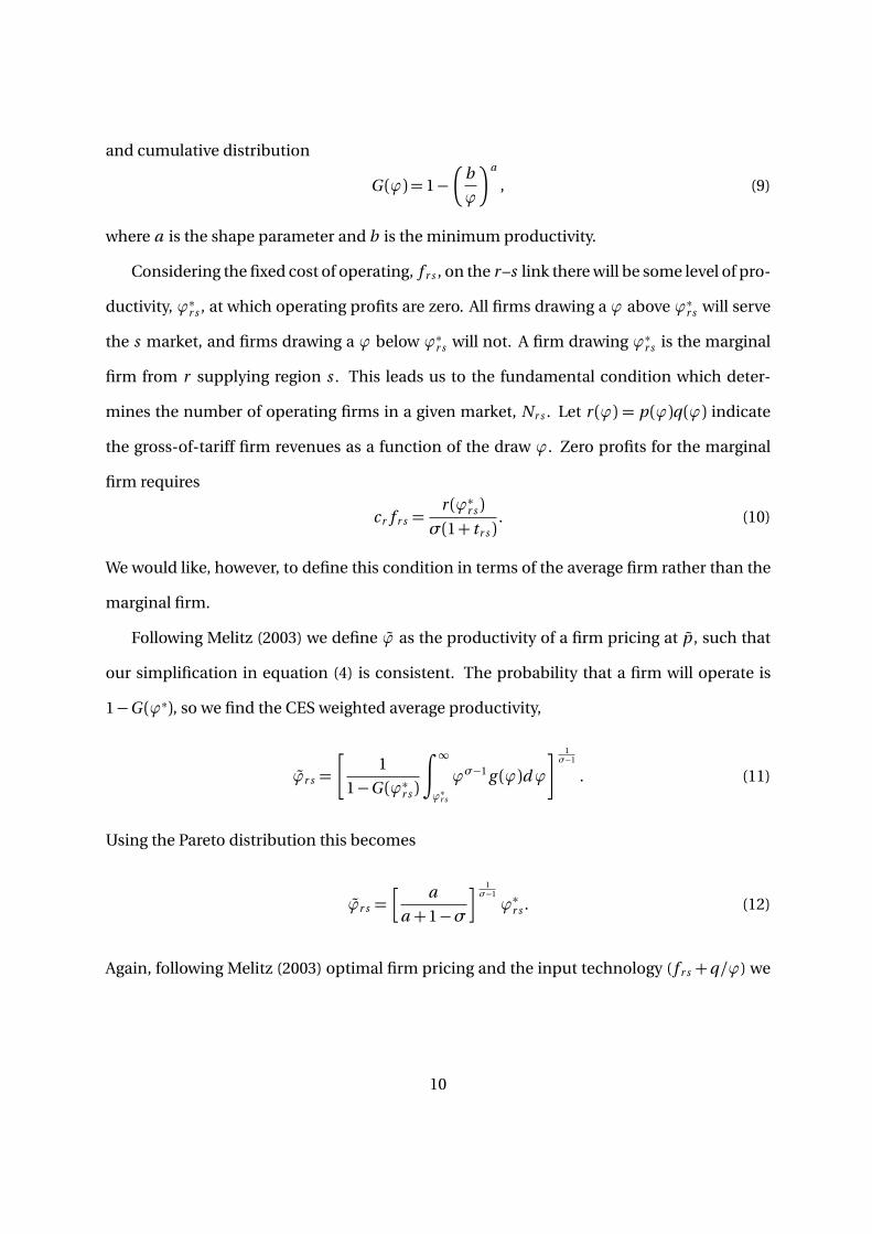
and cumulative distribution

G (ϕ) = 1−

b

ϕ

a

, (9)

where a is the shape parameter and b is the minimum productivity.

Considering the fixed cost of operating, f r s , on the r –s link there will be some level of pro-

ductivity, ϕ∗r s , at which operating profits are zero. All firms drawing a ϕ above ϕ∗r s will serve

the s market, and firms drawing a ϕ below ϕ∗r s will not. A firm drawing ϕ∗r s is the marginal

firm from r supplying region s . This leads us to the fundamental condition which deter-

mines the number of operating firms in a given market, Nr s . Let r (ϕ) = p (ϕ)q (ϕ) indicate

the gross-of-tariff firm revenues as a function of the draw ϕ. Zero profits for the marginal

firm requires

cr f r s =r (ϕ∗r s )σ(1+ tr s )

. (10)

We would like, however, to define this condition in terms of the average firm rather than the

marginal firm.

Following Melitz (2003) we define ϕ as the productivity of a firm pricing at p , such that

our simplification in equation (4) is consistent. The probability that a firm will operate is

1−G (ϕ∗), so we find the CES weighted average productivity,

ϕr s =

1

1−G (ϕ∗r s )

∫ ∞

ϕ∗r s

ϕσ−1 g (ϕ)dϕ

1σ−1

. (11)

Using the Pareto distribution this becomes

ϕr s = a

a +1−σ 1σ−1

ϕ∗r s . (12)

Again, following Melitz (2003) optimal firm pricing and the input technology (f r s +q/ϕ) we

10

establish the relationship between the revenues of firms with different productivity draws:

r (ϕ1)r (ϕ2)

=ϕ1

ϕ2

σ−1

. (13)

Using (12) and (13) to simplify (10) we derive the zero cutoff profit condition in terms of

average-firm revenues and the parameters:

cr f r s +πcr s =

pr s qr s

(1+ tr s )(a +1−σ)

aσ. (14)

The variable πcr s is introduced to track any extra profits that are generated when each of the

M r firms operate in a market. We term these profits capacity rents. The value of πcr s must

be zero in a steady-state, but if M r is sticky a policy shock might lead to Nr s =M r indicating

rents.19

Next we turn to the entry condition which determines the mass of firms, M r . Firm entry

requires a one-time payment of f er , and entered firms face a probability δ in each future

period of a bad shock, which forces exit. In a steady-state equilibrium δM r firms are lost in

a given period so total entry payments in that period must be crδM r f er . From an individual

firm’s perspective the annualized flow of entry payments is crδ f er .

Assuming risk neutrality and no discounting firms enter to the point that expected op-

erating profits equal the entry payment. A firm from r operating in market s can expect to

earn the average profit in that market:

πr s =pr s qr s

σ(1+ tr s )− cr f r s . (15)

Using the zero cutoff profit condition to substitute out the operating fixed cost this reduces

19The value of πcr s is determined by the variational-inequality presented in the next section, equation (20).

We are only concerned with steady-state equilibria in this study, but we found that the computational modelperformed better with the extended condition, which avoids numeric moves where Nr s >M r .

11

to

πr s =pr s qr s

(1+ tr s )(σ−1)

aσ. (16)

The probability that a firm in r will service the s market is simply given by the ratio of

Nr s/M r .20 Setting the firm-level entry-payment flow equal to the expected profits from each

potential market gives us the free entry condition

crδ f er =

∑

s

Nr s

M r

pr s qr s

(1+ tr s )(σ−1)

aσ(17)

which determines the mass of firms, M r .

The final equilibrium conditions establishes the marginal productivity as a function of

the fraction of operating firms, Nr s/M r = 1−G (ϕ∗). Applying the Pareto distribution and

inverting we have

ϕ∗ =b

Nr s

M r

1/a. (18)

In the following section we formalize a computational model based on these fundamental

equilibrium conditions.

4 Solution Method

We represent the policy analysis model on the basis of two related equilibrium problems.

The first is a partial equilibrium (PE) model which captures the heterogeneous-firms indus-

trial organization in manufacturing and the associated impact on productivity and prices.

The PE model takes aggregate income levels and supply schedules as given. The second

module is a constant-returns general equilibrium (GE) model of global trade in all products.

The GE model takes industrial structure as given and determines relative prices, comparative

20In Melitz (2003) the probability that a firm will operate, which equals the fraction of operating firms inequilibrium, is presented as 1−G (ϕ∗).

12

Figure 1: A Decomposition Algorithm

Step 1: Solve one IRTSspatial price equilibriummodel for each commodity

Step 4: Recalibrate resourcesupply schedules and demandfunctions in the PE model.

Step 3: Solve theintegrated CRTS generalequilibrium model

Step 2: Recalibrate Armingtondemand functions in the GE modelto reflect market structure.

-

?

¾

6

advantage and terms of trade. We iterate between these two models in policy simulations,

letting the first module determine industrial structure and the second module establish re-

gional incomes and relative costs. Industrial structure (numbers of firms operating within

and across borders) are passed from the first module to the second whereas the structure of

aggregate demand (income levels and supply prices) are passed back from the GE module to

the PE module. Once the models are mutually consistent we have a solution to the multire-

gion general equilibrium with heterogeneous manufacturing firms. The four steps involved

in the solution algorithm are depicted in Figure 1.

In most policy modeling exercises, applied economists prefer to work with integrated

equilibrium models formulated as systems of equations in which prices and quantities are

determined simultaneously. Indeed, the mixed complementarity format, in which we solve

both the GE and PE modules, is particularly attractive as an integrated framework in which

complementary slackness conditions, e.g. activity analysis, can be readily incorporated along

with conventional neoclassical production functions. In the present application, however,

dimensionality and non-convexities argue strongly in favor of decomposition. When we

solve the industrial organization model on a market by market basis, we avoid dealing with

13

excessively high dimensionalities which otherwise arise when there are large numbers of

both goods and markets. In addition, we find that decomposition leads to a significant im-

provement in robustness of the solution method.

The Melitz model incorporates two types of non-convexity. The first is the conventional

interaction of prices, quantities and incomes. Income effects are the source of most of the

difficulties in proving convergence for the complementarity algorithms. [Mathiesen (1987)].

The second non-convexity is associated with the Dixit-Stiglitz aggregation and productivity

effects. While it is possible to solve general equilibrium models including Dixit-Stiglitz ef-

fects [Markusen (2002)], it is well known that even small instances of the problem class can

be extremely difficult. Our decomposition approach seems to avoid these computational

difficulties by a “divide and conquer” strategy in which income effects are handled in one

submodule and productivity effects in a second module.

4.1 Partial Equilibrium Module

The exogenous links that make the PE module operational are the expenditure levels in each

region, Er , (which establish demand for manufactured goods) and the prices, cr , and quanti-

ties, Yr , of the composite inputs to manufacturing. The model needs some flexibility to react

to shocks, however, so we assume a constant-elasticity input-supply function centered (each

iteration) on the quantity of inputs used by the sector in the general equilibrium (Yr ). Input

supply is thus Yr (cr /cr )η, where η > 0 is the elasticity. If the PE model is consistent with the

general equilibrium cr = cr , where cr satisfies the equilibrium conditions in both modules.

Table 1 summarizes the nonlinear conditions in the PE module and establishes the com-

plementarity between equations and associated variable. In addition to the conditions de-

veloped in the previous section we add the input-market clearance condition (which deter-

14

Table 1: PE module; multiregion heterogeneous-firms partial-equilibrium

Equilibrium Condition (Equation) Associated Variable Dimensions

Zero cutoff profits (ZCP) (14) Nr s : Number of operating firms R ×RFree entry (FE) (17) M r : Mass of firms taking a draw RDixit-Stiglitz preferences (4) Pr : Price index RFirm-level demand (5) qr s : Average-firm quantity R ×RFirm-level pricing (7) pr s : Average-firm price R ×RCES wtd. Average ϕ (11) ϕr s : Average-firm productivity R ×RPareto dist. Marginal ϕ (18) ϕ∗r s : Marginal-firm productivity R ×RInput-market clearance (19) cr : Composite-input price RCapacity constraint (20) πc

r s : Capacity rents R ×RTotal Dimensions: 3R +6R2

mines cr )

Yr

cr

cr

η=δ f e

r M r +∑

s

Nr s

f r s +

qr sτr s

ϕr s

, (19)

and the complementary-slack condition for determining capacity rents (πcr s )

M r −Nr s ≥ 0; πcr s ≥ 0; πc

r s (M r −Nr s ) = 0. (20)

As noted above, in a steady-state equilibrium πcr s will equal zero, but the computational

model benefits from an explicit constraint that prevented numeric moves where Nr s >M r .21

4.2 General Equilibrium Module

The General Equilibrium Module (GE) is formulated as a standard constant-returns model of

world trade in all products. Consumers have preferences over goods differentiated by region

of origin (the Armington assumption). Consider the unit expenditure function associated

with region-s purchases of goods of type k (we reintroduce the commodity index, k ∈ K , in

21This also indicates how the model might be extended into an intertemporal context where M r cannot ad-just instantaneously.

15

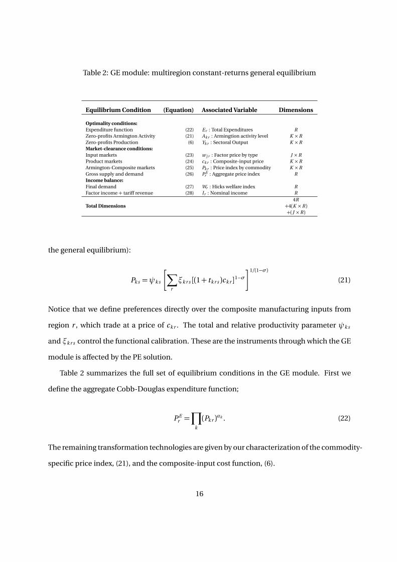
Table 2: GE module: multiregion constant-returns general equilibrium

Equilibrium Condition (Equation) Associated Variable Dimensions

Optimality conditions:Expenditure function (22) Er : Total Expenditures RZero-profits Armington Activity (21) Ak r : Armingtion activity level K ×RZero-profits Production (6) Yk r : Sectoral Output K ×RMarket-clearance conditions:Input markets (23) w j r : Factor price by type J ×RProduct markets (24) ck r : Composite-input price K ×RArmington-Composite markets (25) Pk r : Price index by commodity K ×RGross supply and demand (26) P E

r : Aggregate price index RIncome balance:Final demand (27) Wr : Hicks welfare index RFactor income + tariff revenue (28) Ir : Nominal income R

4RTotal Dimensions +4(K ×R)

+(J ×R)

the general equilibrium):

Pk s =ψk s

∑

r

ξk r s [(1+ tk r s )ck r ]1−σ1/(1−σ)

(21)

Notice that we define preferences directly over the composite manufacturing inputs from

region r , which trade at a price of ck r . The total and relative productivity parameter ψk s

and ξk r s control the functional calibration. These are the instruments through which the GE

module is affected by the PE solution.

Table 2 summarizes the full set of equilibrium conditions in the GE module. First we

define the aggregate Cobb-Douglas expenditure function;

P Er =

∏

k

(Pk r )αk . (22)

The remaining transformation technologies are given by our characterization of the commodity-

specific price index, (21), and the composite-input cost function, (6).

16

Each price (index) has an associated market. Let e j r be the exogenous endowment of

factor j in region r . This will equal the quantity demanded;

e j r =∑

k

βj k r ck r Yk r

w j r. (23)

In turn the supply of the composite-input activity will equal demand (as derived from the

Armington activity):

Yk r =∑

s

ξk r sψk s Ak s

Pk s

(1+ tk r s )ck r

σ. (24)

Supply of the Armington composite equals gross demand:

Ak r =αk Er

Pk r. (25)

Gross expenditures equal the value of final demand plus the value of intermediate use:

Er = P Er Wr +

∑

k

β Ek r ck r Yk r . (26)

The welfare index is calculated directly from ratio of income to the price of the aggregate

commodity:

Wr =Ir

P Er

. (27)

Income in a region equals the value of factor endowments plus tariff revenues:

Is =∑

j

w j s e j s +∑

k

∑

r

tk r sξk r sψk s Ak s

Pk s

(1+ tk r s )ck r

σ. (28)

4.3 Full Solution

The challenge to arriving at a fully consistent general equilibrium is to adjust the ψk s and

ξk r s (where k =Manufacturing) such that aggregate supply of the manufacturing composite

17

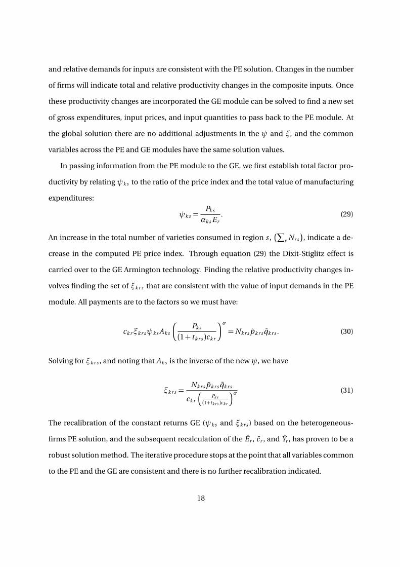
and relative demands for inputs are consistent with the PE solution. Changes in the number

of firms will indicate total and relative productivity changes in the composite inputs. Once

these productivity changes are incorporated the GE module can be solved to find a new set

of gross expenditures, input prices, and input quantities to pass back to the PE module. At

the global solution there are no additional adjustments in the ψ and ξ, and the common

variables across the PE and GE modules have the same solution values.

In passing information from the PE module to the GE, we first establish total factor pro-

ductivity by relatingψk s to the ratio of the price index and the total value of manufacturing

expenditures:

ψk s =Pk s

αk s Er. (29)

An increase in the total number of varieties consumed in region s ,∑

r Nr s

, indicate a de-

crease in the computed PE price index. Through equation (29) the Dixit-Stiglitz effect is

carried over to the GE Armington technology. Finding the relative productivity changes in-

volves finding the set of ξk r s that are consistent with the value of input demands in the PE

module. All payments are to the factors so we must have:

ck rξk r sψk s Ak s

Pk s

(1+ tk r s )ck r

σ=Nk r s pk r s qk r s . (30)

Solving for ξk r s , and noting that Ak s is the inverse of the newψ, we have

ξk r s =Nk r s pk r s qk r s

ck r

Pk s

(1+tk r s )ck r

σ (31)

The recalibration of the constant returns GE (ψk s and ξk r s ) based on the heterogeneous-

firms PE solution, and the subsequent recalculation of the Er , cr , and Yr , has proven to be a

robust solution method. The iterative procedure stops at the point that all variables common

to the PE and the GE are consistent and there is no further recalibration indicated.

18

5 Nonlinear Least-squares Estimation

5.1 Estimation strategy

Consider that the B = 3R + 6R2 nonlinear conditions in the PE module presented above

might be written as F (x ,γ) = 0 which implicitly maps a set of exogenous parameters , γ ∈

RA , to a vector of endogenous variables x ∈ RB . Let γ ∈ RA : A ≤ A denote a vector of

core parameters to be estimated, and let x ∈ RB : B ≤ B denote a key endogenous series

(e.g., bilateral trade flows). Our estimation strategy is to find the γ that minimize the sum of

the squared differences between the log x and observed log x 0 subject to F (x ,γ) = 0 and an

additional A− A direct assumptions about the values of the remaining parameters:

minγ,x (log x − log x 0)T (log x − log x 0)

subject to: F (x ,γ) = 0,

and γ= k ,

where γ are the assumed parameters and k is a vector of constants. We minimize the logged

errors to be consistent with the empirical trade literature, which often assumes a log-linear

form of the trade equation.

We utilize data that is commonly employed in gravity estimations. The economic data

includes gross manufacturing output by region, bilateral trade flows, and measured tariffs.

Because we are interested in fitting a complete general equilibrium (including various non-

manufacturing sectors), we take these data from the Global Trade Analysis Project (GTAP)

[Dimaranan (2006)], a data set commonly employed in general equilibrium simulations of

trade policy changes.22 The GTAP data has been balanced for use in general equilibrium

studies (household income equals expenditure, for example). The data are aggregated to

include nine regions,

22We supplement this with data on international distances from Head and Mayer (2002).

19

CHN China NAF North America LAM Latin AmericaEUR Europe EER Eastern Europe and FSU JKT Jpn, Korea, and TaiwanROA Rest of Asia ANZ Australia and N. Zel. ROW Rest of World ;

and seven aggregate sectors,

AGR Agriculture MTL Mtls-related industry EIS Other Energy IntensiveMFR Manufacturing SER Services ENG EnergyCGD Savings good .

Presently we only estimate the heterogeneous-firms model over the aggregate manufactur-

ing sector (the subscript k is thus suppressed in the remainder of our estimation descrip-

tion). The other sectors in the general equilibrium are assumed competitive and calibrated

via the usual techniques.23

In addition to the economic data we utilize distances between regions to inform trans-

portation costs. Consistent with the gravity literature we assume that iceberg trade costs take

on the following form:

τr s = d θr s ;

where θ is an estimated distance elasticity.24 In addition, we include rent generating ad val-

orem tariffs as measured in the GTAP data, tr s . The c.i.f. import prices, thus, includes the

variable trade costs (1+ tr s )τr s .

Taking the GTAP data as given, and given our assumed structure of trade costs, we have

the following candidates for inclusion in γ:

σ : the inter-variety elasticity of substitutionδ : the probability of firm death,a : shape parameter for the Pareto distribution,b : minimum productivity parameter for Pareto distribution,θ : distance elasticity of iceberg trade costs,f e

r : fixed entry cost,f r s : bilateral fixed cost of shipping from region r to region s .

23We assume an Armington trade structure, with constant returns and perfect competition, in the sectorsother than manufacturing.

24We scale distance such that τ= 1 on the shortest link.

20

Informing these parameters off observed bilateral flows is not meaningful unless we are will-

ing to significantly reduce the parameter space (beyond our implicit assumptions that the

core distribution, substitution, and transport cost parameters are identical across regions).

With R regions there are potentially B =R2 observable flows, but there are at least R2+R+5

parameters. We might eliminateσ from the list of parameters; noting that we are interested

in identifying trade costs conditional on second-order curvature.25 We assume that σ = 3.8

throughout our analysis following the plant-level empirical analysis of Bernard et al. (2003).

In addition, we directly assume the values δ= 0.025, f er = 2, and b = 0.2 following Bernard et

al. (2007).26

The primary assumption that we employ to reduce the parameter space is to impose

structure on the fixed costs. Let f pr be a fixed cost that is specific to goods produced in re-

gion r , and f xs be a fixed cost that is specific to goods exported to region s . Now consider

decomposing the bilateral fixed costs as follows:

f r s = f pr + f x

s + f rr s .

When r = s the f xs term drops out reflecting the idea that f x

s is an outward trade barrier. The

f rr s are idiosyncratic residual bilateral costs. In the initial estimation f r

r s is assumed to be

zero. The number of parameters to be estimated is thus reduced to A = 2n + 2. Essentially,

we are assuming that the expected f rr s is zero. Once the core parameters are estimated, and

locked down, the system can be used to calculate the matrix of residual f rr s which generate

an exact fit on trade flows.27

25Our approach is similar to Anderson and van Wincoop (2003) in that we estimate trade costs conditionalon σ. Alternatively, Hummels (2001) uses direct measures of transportation costs to estimate σ in a gravityframework.

26Bernard et al. (2007) explain that changes in f e rescales the mass of firms where as changes in δ rescale themass of entrants relative to the mass of firms. For consistency we simply adopt their values.

27Balistreri and Hillberry (forthcoming) use a similar technique of stochastic estimation and subsequentexact-fit calibration. This entails a consideration that the econometric residuals might logically be interpretedas idiosyncratic calibration parameters (as opposed to measurement error).

21

5.2 Estimation Results

The primary purpose of our nonlinear estimation is to complete an exact calibration of the

numerical model. This entails a complete enumeration of the structural parameters neces-

sary to reconcile the structural model with observed data. The primary parameters of inter-

est are those that are taken to be common across the world: the shape of the implied Pareto

distribution of productivity draws, a , and the distance elasticity of trade costs, θ . The model

links both these parameters to the geographic pattern of trade.28

We conduct three econometric calibrations of the model. In the first, we allow both θ

and a to be free parameters; they take the values that minimize the econometric objective,

subject to the constraints defined by the model and our choices of the parameters in γ. Very

good estimates of θ appear in the literature, and our second set of estimates constrains the

estimation procedure to replicate a commonly accepted value, θ = 0.27. As a sensitivity

check, our third set of estimates imposes the constraint θ = 0.46.29 Our estimates of key

structural parameters appear in Table 3.30

The interaction between θ and a is a key point of interest. Conditional on the bilateral

trade pattern, our procedure must assign responsibility for trade reductions to these two

parameters (along with the fixed costs).31 Our unconstrained estimate of θ is θ = 0.139,

while a = 5.685. This is a relatively low estimated distance elasticity, and a somewhat high

estimate for the Pareto distribution parameter.32 As we constrain θ to higher values, the

28The link between the geographic pattern of trade and θ is straightforward. Chaney (2006) shows that aexerts a substantial influence on the geography of bilateral trade, via the extensive margin.

29These latter two estimates are taken from Hummels (2001), who estimates θ directly off observed trans-portation cost margins. 0.27 is Hummels’ central estimate, using data from 7 countries that report transportmargins in their international trade statistics. 0.46 is the elasticity of air freight charges with respect to distancein U.S. data, and Hummels uses this as a plausible upper bound on θ . Our unconstrained estimate of θ lieswell below Hummels’ central estimate, and we treat this as a lower bound.

30In order to characterize the degree to which our procedure fits the observed trade pattern, we conduct alog linear regression of observed flows on fitted flows. This regression returns an R2 of 0.946, 0.932, and 0.854for the three specifications, respectively.

31As Chaney (2006) explains, a affects the trade volume via the extensive margin. θ governs the degree towhich prices rise over distance, leading consumers to reduce imports along the intensive margin of trade.

32As noted earlier, Hummels’ central estimate of θ is 0.27. Estimates of a - which are taken from distributions

22

Table 3: Nonlinear estimation results: (dependent variable is log bilateral flows; core fixedparameters areσ= 3.8, δ f e = 0.05, and b = 0.2)

Specificationθ =free θ = 0.27 θ = 0.46

Pareto shape parameter: a 5.685 4.753 3.671(0.810) (0.148) (0.040)

Distance elasticity: θ 0.139 0.27 0.46(0.037)

Source-specific fixed cost: fpr

CHN China 0.837 0.365 5.668(0.422) (0.204) (16.225)

NAF North America 1.314 0.798 68.701(0.630) (0.302) (73.782)

LAM Latin America 0.792 0.139 0.080(0.593) (0.074) (0.041)

EUR Europe 0.792 0.316 2.261(0.358) (0.102) (1.945)

EER Eastern Europe and FSU 1.575 0.282 0.010(0.575) (0.060) (0.006)

JKT Jpn, Korea, and Taiwan 0.153 0.068 0.039(0.206) (0.038) (0.067)

ROA Rest of Asia 0.125 0.024 0.012(0.170) (0.009) (0.005)

ANZ Australia and N. Zel. 0.045 0.031 0.018(0.066) (0.003) (0.030)

ROW Rest of World 3.577 1.539 0.128(1.765) (0.465) (0.050)

Destination-specific fixed cost: f xr

CHN China 4.134 0.551 1.976(2.744) (0.594) (15.066)

NAF North America 0.830 0.018 0.0 bound(0.856) (0.028) (0.021)

LAM Latin America 14.789 3.985 33.463(13.309) (4.822) (14.460)

EUR Europe 1.046 0.062 0.0 bound(0.928) (0.059) (0.005)

EER Eastern Europe and FSU 68.505 51.883 48.791(29.806) (5.905) (2.426)

JKT Jpn, Korea, and Taiwan 0.138 0.096 0.414(0.432) (0.314) (4.605)

ROA Rest of Asia 0.704 0.147 11.814(0.668) (0.254) (19.627)

ANZ Australia and N. Zel. 0.684 0.773 5.146(0.484) (0.504) (17.296)

ROW Rest of World 67.956 97.096 83.177(53.776) (33.536) (5.567)

23

Table 4: Heterogeneity in the productivity distribution: ϕb

for selected values of a

Percentiles50th 75th 90th 95th

Fitted values of aa=5.685 1.130 1.276 1.499 1.694a=4.753 1.157 1.339 1.623 1.878a=3.671 1.208 1.459 1.872 2.262

Implied estimate from Eaton et al. (2004)a=4.2 1.179 1.391 1.730 2.041

Value used in Bernard et al. (2007)a=3.4 1.226 1.503 1.968 2.414

estimated value of a falls. For θ = 0.27, a = 4.753, and for θ = 0.46, a = 3.671.

The lower values of a that occur in our restricted estimates imply greater heterogeneity

in firm productivities. Table 4 illustrates some features of the productivity distributions im-

plied by different values of a . For our unconstrained estimate of a , a firm with a productivity

draw at the median of the distribution would be 1.130 times as productive as a firm with

the minimum draw. As a falls, the productivity distribution flattens out. In our subsequent

counterfactual scenarios, we will be employing the constrained estimate a = 4.753, the es-

timate corresponding to θ = 0.27. In this case, the median productivity draw is 1.157 times

the size of the minimum draw.

The structural estimation results in Table 3 also contain estimated values of source- and

destination-specific fixed costs. In the data, regions will differ in the share of manufacturing

output that they export.33 Structural estimation attributes such variation largely to variation

in the source-specific fixed cost f pr . The lowest of these estimated costs appear to be in Rest

of Asia (ROA) and Australia and New Zealand (ANZ). Both relative and absolute estimates of

fixed production costs vary with θ and a .34

of plant/firm level market shares - vary, and are conditional on a choice of σ. Bernard et al. (2007) choose a =3.4, and the estimates in Eaton et al. (2004) imply a = 4.2 under our maintained assumption thatσ= 3.8.

33Some of the observed variation in this statistic will arise because regions vary in their non-manufacturingsectors’ use of manufacturing output. Our structural estimation procedure maintains these idiosyncrasiesthroughout calibration, so variation of this sort does not pollute the estimates of f p

r .34Standard errors for the estimated fixed costs are generally tighter when the distance elasticity is fixed. Fix-

ing θ allows a to be more precisely estimated (exploiting any unexplained variation in the distance elasticity of

24

The fitting procedure also defines fitted destination-specific fixed costs, f xr . These pa-

rameters are largely identified off of observed home bias in fitted trade flows, conditional

on the other structural parameters. The estimates reported here suggest relatively low fixed

costs of importing to the most developed regions in the data. Recall that the GTAP tariff data

are included in the calibration, so these are best interpreted as implicit non-tariff barriers to

trade (averaged across origins).35

Our non-linear estimating system fits the data in a manner quite similar to a conven-

tional gravity equation. An OLS regression of log(x ) on (logged) d r s , (1 + tr s ), ( fpr + f x

s ),

ck r Yk r , αk Es , and Ps returns a perfect fit. This intuitive OLS specification relies, of course,

on our non-linear estimates of f pr , f x

s , and Ps .36 Following Hillberry and Hummels (forth-

coming) we decompose trade flows into extensive and intensive margins, regressing log Nr s

and pr s qr s on the determinants of bilateral trade. We report these results in Table 5. The re-

sults show that average firm revenues (c.i.f.) rise in tandem with tariffs and fixed trade costs,

while all other responses to bilateral trade are observed as changes in the number of firms

serving a particular market.37

Once the core parameters reported in Table 3 are established we can freeze these at their

point estimates and find a set of residual bilateral costs, f rr s , that give us perfect consis-

trade, for example). More precise estimates of a allow more precise estimates of the fixed costs in the model.35These and subsequent estimates take the rather extreme view that any unexplained reduction in fitted

trade volumes should be attributed to trade costs of one type or another. This interpretation is in keeping withmuch of the geography-of-trade literature. The trade policy literature typically focuses only on known tradebarriers, and attributes unexplained variation in trade flows to Armington distribution parameters. Balistreriand Hillberry (forthcoming) explain that these two approaches are best understood as different identificationstrategies for fitting the trade pattern.

36The fitted values of trade in the regression are fully consistent with optimizing behaviour of the agentsin the model. As Helpman et al. (2007) show, a Pareto distribution for firm heterogeneity coupled with anassumption that fixed costs are exporter- and importer-specific (which is true in the case of our fitted values)generates a multiplicative gravity relationship (and thus a perfect fit in a properly specified log-linear regressionof structurally fitted flows on dependent variables). The estimates here link the flows to variables that appearin the general equilibrium model, rather than to a summary measure like “outward multilateral resistance” asdescribed in Anderson and van Wincoop (2004).

37Note that the implications for the intensive margin follow directly from 15. The estimated elasticities forthe extensive margin are not directly interpretable in terms of the structural parameters because the right handside variables are correlated.

25

Table 5: Intensive and Extensive Margins in Fitted Bilateral Trade Flows

θ = f r e e θ = 0.27 θ = 0.46Nr s pr s qr s Nr s pr s qr s Nr s pr s qr s

Regressord r s -0.790 0 -1.282 0 -1.687 0

(0.001) (0) (0.001) (0) (0.001) (0)(1+ tr s ) -7.761 1 -6.495 1 -5.014 1

(0.019) (0) (0.020) (0) (0.019) (0)( f p

r + f xs ) -2.028 1 -1.696 1 -1.311 1

(0.001) (0) (0.001) (0) (0.000) (0)ck r Yk r 1.005 0 1.005 0 1.010 0

(0.001) (0) (0.001) (0) (0.001) (0)αk s Es 2.028 0 1.696 0 1.312 0

(0.002) (0) (0.002) (0) (0.001) (0)Ps 5.674 0 4.746 0 3.674 0

(0.008) (0) (0.006) (0) (0.004) (0)constant -12.671 2.013 -10.269 2.224 -7.438 2.773

(0.012) (0) (0.010) (0) (0.008) (0)Note: All variables are in natural logarithms. All regressions have 81

observations and R2 = 1.

Table 6: Residual Bilateral Fixed Trade Costs (f rr s )

DestinationCHN NAF LAM EUR EER JKT ROA ANZ ROW

SourceCHN -0.245 -0.295 -3.509 0.260 -34.552 -0.021 1.785 0.139 -4.099NAF -0.968 0.029 -3.305 0.160 38.416 -0.551 -0.532 -0.885 44.506LAM -0.529 0.086 -0.106 0.057 -49.168 -0.041 -0.146 1.427 -49.640EUR -0.606 0.015 -3.263 0.169 -42.761 -0.013 -0.026 -0.798 -12.545EER -0.429 0.578 -0.823 -0.092 -0.189 0.282 1.057 0.957 28.764JKT -0.398 0.020 -3.728 0.226 -24.245 -0.032 0.059 -0.353 -44.077ROA -0.131 -0.015 -3.251 0.040 -31.674 0.014 6.9E-4 -0.198 -48.578ANZ -0.428 0.001 -3.421 -0.048 -44.719 -0.108 -0.010 -0.003 -78.569ROW 0.411 -1.047 4.404 -0.424 -24.817 0.016 1.067 1.230 0.012

26

Table 7: Total Bilateral Fixed Trade Costs (f r s )

DestinationCHN NAF LAM EUR EER JKT ROA ANZ ROW

SourceCHN 0.120 0.087 0.840 0.686 17.697 0.440 2.297 1.277 93.362NAF 0.381 0.827 1.478 1.020 91.097 0.343 0.414 0.686 142.400LAM 0.160 0.242 0.032 0.257 2.853 0.194 0.140 2.338 47.594EUR 0.261 0.349 1.038 0.485 9.439 0.399 0.437 0.291 84.867EER 0.405 0.878 3.444 0.252 0.093 0.660 1.487 2.013 126.142JKT 0.221 0.105 0.324 0.356 27.706 0.036 0.274 0.488 53.086ROA 0.444 0.026 0.758 0.126 20.233 0.134 0.024 0.599 48.542ANZ 0.154 0.050 0.594 0.045 7.195 0.018 0.168 0.028 18.558ROW 2.501 0.509 9.927 1.176 28.605 1.651 2.753 3.541 1.550

tency with observed trade flows.38 We report these estimates for the constrained estimates

(θ = 0.27) in Table 6. From the perspective of the nonlinear estimation these are effectively

econometric residuals—they allow the structure to fit the data exactly. Alternatively, from

the perspective performing theory consistent counterfactual analysis they are idiosyncratic

calibration parameters.39

Table 7 shows the full matrix of total bilateral fixed costs including the residual plus the

source and destination charges. So, for example, we might consider that import penetration

into EER is difficult, but it is particularly difficult for North American firms. On this partic-

ular link the total fixed cost of 91.1 is nearly twice as large as the base destination charge to

get into EER, 51.9. The fixed costs into ROW are also large, but this is attributable to aggrega-

tion bias, as this region represents many small economies.40 Variation in the estimated f r s

explains 12 percent of the variation in bilateral trade flows.

38There are a number of potential matrices of residual fixed costs that are consistent with observed trade andthe estimated parameters. We choose the one that minimizes the squared residual bilateral costs.

39Hillberry et al. (2005) show the usefulness of framing standard general-equilibrium calibration exercisesas the systematic identification of idiosyncratic residual parameters. As in any standard econometric exercisethese residual parameters are useful indicators of model fit.

40When we assume that the ROW aggregate is a large integrated market, large fixed costs are needed to explainthe relatively low volume of trade.

27

Table 8: Counterfactual Welfare Impacts (% Equivalent Variation)

ScenarioA B C D

CRTS-Tariff Tariff Fix Cost Both

RegionCHN 0.3 1.3 3.3 5.2NAF -0.0 0.0 0.7 0.8LAM 0.1 0.5 1.6 2.4EUR 0.1 0.2 1.3 1.7EER -0.1 -0.3 4.3 4.6JKT 0.1 0.3 1.9 2.2ROA 0.3 1.1 5.3 6.5ANZ 0.4 1.4 2.2 4.3ROW -0.2 -0.7 2.4 1.9

6 Counterfactual Simulations

We analyze four scenarios that compare the impacts of tariff and fixed cost reductions:

(A) Armington constant-returns formulation with a 50% reduction in manufacturing tariffs;

(B) Heterogeneous-firms model with a 50% reduction in manufacturing tariffs;

(C) Heterogeneous-firms model with a 50% reduction in fixed trade costs; and

(D) Heterogeneous-firms model with both the tariff and fixed cost cuts.

Scenario (A) is a reference case where we assume a standard Armington trade structure and

constant-returns production.41 Table 8 shows welfare changes induced by the tariff cut. Al-

though most regions gain from the tariff cuts, three regions suffer welfare losses (NAF, EER,

and ROW).42 Examining the same tariff cuts in the heterogeneous-firms model (Scenario B)

indicates substantially greater gains. Taking the simple-average welfare change across re-

gions the heterogeneous-firms structure indicates welfare gains from liberalization that are

nearly four times larger than in the baseline case. The simple-average welfare gain of 0.4% in

41We simply run the tariff cut on the GE module without making the iterative productivity adjustments. Thisgives us a perfectly comparable constant-returns benchmark to judge the performance of the new theory.

42This is not particularly surprising. At low substitution elasticities (3.8 in this case) the Armington structureimplies high optimal tariffs, so the benchmark tariff structure is likely to benefit some regions.

28

Scenario B may not seem particularly impressive, but consider the following statistics from

our aggregation of the GTAP data: gross manufacturing output is only 26% of world gross

output, only 15% of manufacturing output is traded to another region, and the simple aver-

age benchmark tariff on these flows is only 9.3%. So the typical tariff cut is less than 5%, and

applies to less than 4% of gross output. In this context, an average welfare gain of 0.4% seems

quite large. With the exception of the ROW and EER regions, tariff cuts in the heterogeneous-

firms structure produce larger net welfare gains than the constant returns benchmark.

In Scenario (C) we examine a 50% cut in the fixed costs associated with non-domestic

trade links. This generates important gains across the board. The results are consistent with

a recent trade literature focussing on the relative importance of unobserved (non-tariff) bar-

riers and tariffs.43 In Scenario (D) both the tariff and fixed cost reductions are combined.

There are considerable increases in welfare under Scenario (D) considering that Manufac-

turing is the only sector being liberalized. The simple-average welfare gain under Scenario

(D) is nearly 30 times larger than in the Armington reference case. Notice also that fixed-cost

(or non-tariff barrier) reductions often complement tariff cuts. Absolute welfare increases of

1% to 6% are considerably larger than most computational estimates.44

As noted above, one of the key critiques of current policy simulation models is that they

fail to account for the productivity growth associated with liberalization. Table 9 indicates

the simulated gains in average productivity across firms active in their respective domestic

markets. Consistent with the arguments put forward by the proponents of the heterogeneous-

firms model, our simulations show productivity gains due to liberalization. Increased ex-

posure to external markets, whether induced by a reduction in tariff or non-tariff barriers,

induces productivity growth.

The other key component of the model is that trade policy affects the extensive margin.

The number of foreign varieties increases when trade costs fall. The threshold for import

43Anderson and van Wincoop (2004)44See Rutherford and Tarr (2002).

29

Table 9: Domestic-firm Productivity Growth (% Change)

ScenarioB C D

Tariff Fix Cost Both

RegionCHN 0.8 1.5 2.7NAF 0.3 1.1 1.6LAM 1.1 1.5 3.2EUR 0.4 1.7 2.3EER 0.8 3.1 4.2JKT 0.6 1.6 2.6ROA 1.3 3.4 5.5ANZ 2.1 3.1 6.5ROW 0.6 1.6 2.5

penetration falls and more foreign firms find it profitable to enter a given market. In contrast,

the effect of changes in trade costs on the number of domestic varieties is not clear. As Melitz

(2003) explains there are two mechanisms by which the distribution of operational firms in

a given country changes with trade. First, the number of exporting firms increases and the

profits of all exporting firms increase, which induces entry of new varieties. The increased

activity of these firms, however, bid up the input price. Thus, the second effect acts to induce

exit of varieties with low productivity realizations.

On net, however, consumers will likely benefit from lost domestic varieties because fac-

tor returns increase and the remaining domestic varieties are less expensive. More produc-

tive firms optimally price lower, so eliminating low productivity firms depresses the average

price. All of the variety and price effects can be summarized in the solution price index on

manufactured goods, Pr . Table 10 presents the percentage change in the price index across

the scenarios. Further, we break out the variety effects in Table 11. Although the number of

overall varieties falls for many regions, trade growth on the extensive margin combined with

lower domestic prices result in lower overall price indexes.

30

Table 10: Manufacturing Price Index, Pr (% Change)

ScenarioB C D

Tariff Fix Cost Both

RegionCHN 0.8 -0.9 -0.9NAF -0.2 -1.7 -2.2LAM -0.7 -2.4 -3.5EUR 0.2 -1.3 -1.5EER -0.9 -3.8 -5.0JKT 0.3 0.4 -0.1ROA -0.5 -2.0 -3.3ANZ 0.4 -2.6 -3.3ROW -2.2 -3.5 -5.6

7 Conclusion

A broad body of empirical literature documents persistent differences in plant-level produc-

tivity. This literature has also shown that the reallocation of production activities, from less-

to more-productive plants, is an important part of aggregate productivity growth. These ba-

sic characteristics of industrial organization have important implications for international

trade and commercial policy. The unifying theory proposed by Melitz (2003) offers insights

into these implications. Our contribution is to present a quantitative assessment of the ef-

fects of this new richer structure on simulated policy analysis. We illustrate that relatively

modest liberalization generates substantial gains due to the predicted endogenous produc-

tivity improvements.

In the case of a 50% reduction in tariffs on traded manufactured goods the simple-average

welfare gains are on the order of 4 times greater when we consider the new theory. These

gains are complemented, and compounded, by reductions in the fixed costs. When we add a

50% reduction in cross-border fixed costs to the tariff cuts the welfare gains grow to roughly

30 times what is measured in the constant-returns reference liberalization.

31

Table 11: Changes in the Number of Operating Firms, Nr s (% Change)

ScenarioB C D

Tariff Fix Cost Both

Imported Varieties(extensive margin):

CHN 30.4 200.3 287.1NAF 12.5 162.3 198.4LAM 29.1 167.0 248.8EUR 16.7 190.4 237.1EER 13.9 175.6 215.8JKT 39.3 229.7 346.1ROA 22.9 203.2 264.4ANZ 28.5 179.4 247.7ROW 12.8 157.5 198.1

Domestic Varieties:CHN -2.2 -5.1 -8.3NAF -1.2 -5.1 -6.9LAM -4.1 -6.6 -12.2EUR -1.6 -7.1 -9.2EER -3.3 -9.9 -13.8JKT -2.3 -7.3 -10.7ROA -4.6 -12.6 -18.9ANZ -7.3 -14.1 -22.3ROW -2.8 -5.7 -9.6

Total Varieties:CHN -0.3 6.9 9.0NAF 6.5 89.3 108.9LAM -3.8 -5.5 -10.5EUR 2.0 31.2 38.5EER -3.3 -9.3 -13.1JKT -1.4 -1.9 -2.5ROA -4.0 -8.0 -12.9ANZ -6.5 -9.8 -16.4ROW -2.7 -5.0 -8.7

32

Some truth in advertising is in order for our results. First, we employ a novel, if not rad-

ical, method for measuring unobserved fixed costs. We depart from the econometric litera-

ture by employing a nonlinear estimation that includes the extensive-form general equilib-

rium conditions as side constraints. Our focus is on arriving at fitted values, while maintain-

ing complete consistency between the econometric and simulation models. Our estimation

method is also a stark departure from traditional calibration methods used to fit simulation

models; we do not allow preference-bias parameters to drive trade. The onus of explaining

the observed pattern of trade is on the theory and the standard parameters that appear in the

theory, not on added preference-bias parameters. The very large fixed costs that we estimate

are open to criticism, and we view them as crude indicators of how big the barriers may be.45

It is generally accepted by economists that unobserved trade costs are an important com-

ponent of the world trade equilibrium. We follow one of the few paths available, which is to

accept the structure fully and use it to inform unobservables from the observables.

The second major caveat that we place on our results involves the data. We accept the

GTAP data as given and further aggregate it. This is useful in terms of reducing computa-

tional complexity and in allowing us to efficiently summarize reports. The GTAP data are

balanced; they have already been fitted to a set of fundamental accounting identities. The

data are consistent with general-equilibrium adding-up restrictions, but the original fitting

procedure weakens the validity of any statistical inference that one might draw from our

estimation.

The usual aggregation biases abound in our data, and we have additional concerns given

the theory’s focus on firm-level behavior. Our aggregate manufacturing sector is not a satis-

fying definition of an industry or product. Regional aggregation is also problematic. The ag-

gregate rest-of-world region is actually numerous small disjoint markets rather than a large

45These estimates are not open the critique leveled by Balistreri and Hillberry (2006), because the fixed costsmeasured here impinge on missing trade not existing trade. Firms choked out of a market due to fixed costs donot incur the fixed costs. The payment of these costs is therefore not observed.

33

integrated market. We probably overstate the fixed costs of entering the rest-of-world region

because these are necessary for explaining the relative lack of trade with what appears to be

a large region.

We thus present our estimates conditional on the particular aggregation of the data, the

assumed structure, and our maintained hypotheses about key structural parameters. We

see important extensions in the area of regional and industry disaggregation. Future re-

search will also need to tackle the issue of consistent structural estimation. We are somewhat

unique in our development of an econometric method that facilitates directly, and fully con-

sistent, welfare analysis of policy. Others may find this departure from standard regression

analysis useful and relevant. We are firmly within the empirical-trade tradition, which places

theory, not established statistical methods, as the foundation for analysis. Given the rich na-

ture of contemporary theory we hope our empirical welfare analysis encourages others to

continue developing the literature in this direction.

References

Anderson, James, and Eric van Wincoop (2003) ‘Gravity with gravitas: A solution to the bor-der puzzle.’ American Economic Review 93(1), 170–192

(2004) ‘Trade costs.’ Journal of Economic Literature 42(3), 691–751

Anderson, Kym, William J. Martin, and Dominique van der Mensbrugghe (2005) ‘Global im-pacts of the Doha scenarios on poverty.’ World Bank Policy Research Working Paper Series3735

Aw, Bee Yan, Sukkyun Chung, and Mark J. Roberts (2000) ‘Productivity and turnover in theexport market: Micro evidence from Taiwan and South Korea.’ World Bank Economic Re-view

Aw, Bee Yan, Xiaomin Chen, and Mark J. Roberts (2001) ‘Firm-level evidence on productiv-ity differentials and turnover in Taiwanese manufacturing.’ Journal of Development Eco-nomics 66, 51–86

Balistreri, Edward J., and Russell H. Hillberry (2006) ‘Trade frictions and welfare in the gravitymodel: How much of the iceberg melts?’ Canadian Journal of Economics 39(1), 247–265

34

(2007) ‘Structural estimation and the border puzzle.’ Journal of International Economics72(2), 451–463

(forthcoming) ‘The gravity model: An illustration of structural estimation as calibration.’Economic Inquiry

Bartelsman, Eric J., and Mark Doms (2000) ‘Understanding productivity: Lessons from lon-gitudinal microdata.’ Journal of Economic Literature 38(3), 569–594

Bartelsman, Eric J., and Phoebus J. Dhrymes (1998) ‘Productivity dynamics: U.S. manufac-turing plants 1972-1986.’ Journal of Productivity Analysis 9(1), 5–34

Bernard, Andrew, and J. Bradford Jensen (1999) ‘Exceptional exporter performance: Cause,effect, or both?’ Journal of International Economics 47(1), 1–25

Bernard, Andrew B., J. Bradford Jensen, and Peter K. Schott (2006) ‘Trade costs, firms andproductivity.’ Journal of Monetary Economics 53(5), 917–937

Bernard, Andrew B., Jonathan Eaton, J. Bradford Jensen, and Samuel Kortum (2003) ‘Plantsand productivity in international trade.’ American Economic Review 93, 1268–1290

Bernard, Andrew B., Stephen Redding, and Peter K. Schott (2007) ‘Comparative advantageand heterogeneous firms.’ Review of Economic Studies 74, 31–66

Broda, Christian, and David E. Weinstein (2006) ‘Globalization and the gains from variety.’Quarterly Journal of Economics 121(2), 541–585

Chaney, Thomas (2006) ‘Distorted gravity: Heterogeneous firms, market structure and thegeography of international trade.’ mimeo, University of Chicago

Clerides, Sofronis, Saul Lach, and James Tybout (1998) ‘Is learning by importing important?micro-dynamic evidence from Colombia, Mexico and Morocco.’ Quarterly Journal of Eco-nomics 113(3), 903–947

DeBaere, Peter, and Shalah Mostashari (2006) ‘Do tariffs matter for the extensive margin ofinternational trade? An empirical analysis.’ University of Texas, mimeo

Dimaranan, Betina V. (Editor) (2006) Global Trade, Assistance, and Production: The GTAP 6Data Base (West Lafayette: Center for Global Trade Analysis, Purdue University)

Eaton, Jonathan, Samuel Kortum, and Francis Kramarz (2004) ‘Dissecting trade: Firms, in-dustries and export destinations.’ American Economic Review 94(2), 150–154

Evenett, Simon, and Anthony Venables (2002) ‘Export growth in developing countries: Mar-ket entry and bilateral trade flows.’ mimeo, University of St. Gallen

35

Foster, Lucia, John Haltiwanger, and C.J. Krizan (2001) ‘Aggregate productivity growth:Lessons from the microeconomic evidence.’ In New Directions in Productivity Analysis,ed. Edward Dean, Michael Harper, and Charles Hulten (University of Chicago Press)

Haveman, John, and David Hummels (2004) ‘Alternative hypotheses and the volume of trade:The gravity equation and the extent of specialization.’ Canadian Journal of Economics37(1), 199–218

Head, Keith, and Thierry Mayer (2002) ‘Illusory border effects: Distance mismeasurementinflates estimates of home bias in trade.’ CEPII working paper 2002-01

Helpman, Elhanan, Marc Melitz, and Yona Rubinstein (2007) ‘Trading partners and tradingvolumes.’ NBER Working Paper 12927

Hillberry, Russell, and David Hummels (forthcoming) ‘Trade responses to geographic fric-tions: A decomposition using micro-data.’ European Economic Review

Hillberry, Russell H., Michael A. Anderson, Edward J. Balistreri, and Alan K. Fox (2005) ‘Tasteparameters as model residuals: Assessing the ‘fit’ of an Armington trade model.’ Review ofInternational Economics 13(5), 973–984

Hummels, David (2001) ‘Toward a geography of trade costs.’ mimeo, Purdue University

Hummels, David, and Peter Klenow (2005) ‘The variety and quality of a nation’s exports.’American Economic Review 95(3), 704–723

Kehoe, Timothy J. (2005) ‘An evaluation of the performance of applied general equilibriummodels of the impact of NAFTA.’ In Frontiers in Applied General Equilibrium Modeling:Essays in Honor of Herbert Scarf, ed. Timothy J. Kehoe, T.N. Srinivasan, and John Whalley(Cambridge University Press) pp. 341–377

Kehoe, Timothy J., and Kim J. Ruhl (2002) ‘How important is the new goods margin in inter-national trade?’ mimeo, University of Minnesota

Markusen, J.R. (2002) Multinational Firms and the Theory of International Trade (Cam-bridge: MIT Press)

Mathiesen, Lars (1987) ‘An algorithm based on a sequence of linear complementarity prob-lems applied to a walrasian equilibrium model: An example.’ Mathematical Programmingpp. 1–18

Melitz, Marc J. (2003) ‘The impact of trade on intra-industry reallocations and aggregate in-dustry productivity.’ Econometrica 71(6), 1695–1725

Pavcnik, Nina (2002) ‘Trade liberalization, exit, and productivity improvement: Evidencefrom Chilean plants.’ Review of Economic Studies 69(1), 245–276

36

Roberts, Mark J., and James Tybout (1997) ‘The decision to export in Columbia: An empiricalmodel of entry with sunk costs.’ American Economic Review 87(4), 545–564

Romer, Paul M. (1994) ‘New goods, old theory, and the welfare costs of trade restrictions.’Journal of Development Economics 43(1), 5–38

Rutherford, Thomas F., and David G. Tarr (2002) ‘Trade liberalization, product variety andgrowth in a small open economy: a quantitative assessment.’ Journal of International Eco-nomics 56(2), 247–272

United States Trade Representative (2005) ‘Report to the Congress on the extension of TradePromotion Authority: Annex 3’

37