Full-Information Estimation of Heterogeneous AgentModels Using Macro and Micro Data

Laura Liu Mikkel Plagborg-Møller∗Indiana University Princeton University

First version: December 19, 2018This version: January 12, 2021

Abstract: We develop a generally applicable full-information inference methodfor heterogeneous agent models, combining aggregate time series data and re-peated cross sections of micro data. To handle unobserved aggregate state vari-ables that affect cross-sectional distributions, we compute a numerically unbiasedestimate of the model-implied likelihood function. Employing the likelihood es-timate in a Markov Chain Monte Carlo algorithm, we obtain fully efficient andvalid Bayesian inference. Evaluation of the micro part of the likelihood lends it-self naturally to parallel computing. Numerical illustrations in models with het-erogeneous households or firms demonstrate that the proposed full-informationmethod substantially sharpens inference relative to using only macro data, andfor some parameters micro data is essential for identification.

Keywords: Bayesian inference, data combination, heterogeneous agent modelsJEL codes: C11, C32, E1

∗lauraliu@iu.edu (Liu) and mikkelpm@princeton.edu (Plagborg-Møller). We are grateful for help-ful comments from Adrien Auclert, Yoosoon Chang, Marco Del Negro, Simon Mongey, Hyungsik RogerMoon, Ulrich Müller, Jonathan Payne, Frank Schorfheide, Neil Shephard, Thomas Winberry, and seminarparticipants at Chicago, FRB Chicago, FRB Cleveland, FRB NY, FRB Philadelphia, NYU, Princeton, UNC-Chapel Hill, the Midwest Econometrics Group Conference, the USC Dornsife INET Conference on PanelData Forecasting, the NBER-NSF Seminar on Bayesian Inference in Econometrics and Statistics, the NBERSummer Institute, and the World Congress of the Econometric Society. Plagborg-Møller acknowledges thatthis material is based upon work supported by the NSF under Grant #1851665. Any opinions, findings, andconclusions or recommendations expressed in this material are those of the authors and do not necessarilyreflect the views of the NSF.

1

1 Introduction

Macroeconomic models with heterogeneous agents have exploded in popularity in recentyears.1 New micro data sets – including firm and household surveys, social security and taxrecords, and censuses – have exposed the empirical failures of traditional representative agentapproaches. The new models not only improve the fit to the data, but also make it possibleto meaningfully investigate the causes and consequences of inequality among householdsor firms along several dimensions, including endowments, financial constraints, age, size,location, etc.

So far, however, empirical work in this area has only been able to exploit limited featuresof the micro data sources that motivated the development of the new models. As emphasizedby Ahn, Kaplan, Moll, Winberry, and Wolf (2017), the burgeoning academic literature hasmostly calibrated model parameters and performed over-identification tests by matching afew empirical moments that are deemed important a priori. This approach may be highlyinefficient, as it ignores that the models’ implied macro dynamics and cross-sectional proper-ties often fully determine the entire distribution of the observed macro and micro data. Thefailure to exploit the joint information content of macro and micro data stands in stark con-trast to the well-developed inference procedures for estimating representative agent modelsusing only macro data (Herbst and Schorfheide, 2016).

To exploit the full information content of macro and micro data, we develop a generaltechnique to perform Bayesian inference in heterogeneous agent models. We assume theavailability of aggregate time series data as well as repeated cross sections of micro data.Evaluation of the joint macro and micro likelihood function is complicated by the fact thatthe model-implied cross-sectional distributions typically depend on unobserved aggregatestate variables. To overcome this problem, we devise a way to compute a numerically un-biased estimate of the model-implied likelihood function of the macro and micro data. Asargued by Andrieu, Doucet, and Holenstein (2010) and Flury and Shephard (2011), suchan unbiased likelihood estimate can be employed in standard Markov Chain Monte Carlo(MCMC) procedures to generate draws from the fully efficient Bayesian posterior distributiongiven all available data.

The starting point of our analysis is the insight that existing solution methods for hetero-geneous agent models directly imply the functional form of the joint sampling distribution of

1For references and discussion, see Krueger, Mitman, and Perri (2016), Ahn, Kaplan, Moll, Winberry,and Wolf (2017), and Kaplan and Violante (2018).

2

macro and micro data, given structural parameters. These models are typically solved nu-merically by imposing a flexible functional form on the relevant cross-sectional distributions(e.g., a discrete histogram or parametric family of densities). The distributions are governedby time-varying unobserved state variables (e.g., moments). To calculate the model-impliedlikelihood, we decompose it into two parts. First, heterogeneous agent models are typicallysolved using the method of Reiter (2009), which linearizes with respect to the macro shocksbut not the micro shocks. Hence, the macro part of the likelihood can be evaluated usingstandard linear state space methods, as proposed by Mongey and Williams (2017) and Win-berry (2018).2 Second, the likelihood of the repeated cross sections of micro data, conditionalon the macro state variables, can be evaluated by simply plugging into the assumed cross-sectional density. The key challenge that our method overcomes is that the econometriciantypically does not directly observe the macro state variables. Instead, the observed macrotime series are imperfectly informative about the underlying states.

Our procedure can loosely be viewed as a rigorous Bayesian version of a two-step ap-proach: First we estimate the latent macro states from macro data, and then we computethe model-implied cross-sectional likelihood conditional on these estimated macro states.More precisely, we obtain a numerically unbiased estimate of the likelihood by averagingthe cross-sectional likelihood across repeated draws from the smoothing distribution of thehidden states given the macro data. We emphasize that, despite being based on a likelihoodestimate, our method is fully Bayesian and automatically takes into account all sources ofuncertainty about parameters and states. An attractive computational feature is that evalu-ation of the micro part of the likelihood lends itself naturally to parallel computing. Hence,computation time scales well with the size of the data set.

We perform finite-sample valid and fully efficient Bayesian inference by plugging theunbiased likelihood estimate into a standard MCMC algorithm. The generic arguments ofAndrieu, Doucet, and Holenstein (2010) and Flury and Shephard (2011) imply that theergodic distribution of the MCMC chain is the full-information posterior distribution thatwe would have obtained if we had known how to evaluate the exact likelihood function (notjust an unbiased estimate of it). This is true no matter how many smoothing draws are usedto compute the unbiased likelihood estimate. In principle, we may use any MCMC posteriorsampling algorithm that relies only on evaluating (the unbiased estimate of) the posteriordensity, such as Random Walk Metropolis-Hastings.

2If non-Reiter model solution methods are used, our general estimation approach could in principle stillbe applied, though its computational feasibility would be context-dependent, as discussed in Section 6.

3

In contrast to other estimation methods, our full-information method is automaticallyfinite-sample efficient and can easily handle unobserved individual heterogeneity, micro mea-surement error, as well as data imperfections such as selection or censoring. In an importantearly work, Mongey and Williams (2017) propose to exploit micro data by collapsing it totime series of cross-sectional moments and incorporating these into the macro likelihood. Inprinciple, this approach can be as efficient as our full-information approach if the structuralmodel implies that these moments are sufficient statistics for the micro data. We provideexamples where this is not the case, for example due to the presence of unobserved individualheterogeneity and/or micro measurement error. Even when sufficient statistics do exist, itis necessary to properly account for sampling error in the observed cross-sectional moments,which is done automatically by our full-information likelihood method, but could be delicateand imprecise for moment-based approaches. Moreover, textbook adjustments to the microlikelihood allow us to accommodate specific empirically realistic features of micro data suchas selection (e.g., over-sampling of large firms) or censoring (e.g., top-coding of income),whereas this is challenging to do efficiently with moment-based approaches.

We illustrate the joint inferential power of macro and micro data through two numericalexamples: a heterogeneous household model (Krusell and Smith, 1998) and a heterogeneousfirm model (Khan and Thomas, 2008). In both cases we assume that the econometricianobserves certain standard macro time series as well as intermittent repeated cross sectionsof, respectively, (i) household employment and income and (ii) firm capital and labor inputs.Using simulated data, and given flat priors, we show that our full-information method ac-curately recovers the true structural model parameters. Importantly, for several structuralparameters, the micro data reduces the length of posterior credible intervals substantially,relative to inference that exploits only the macro data. In fact, we give examples of pa-rameters that can only be identified if micro data is available. In contrast, inference frommoment-based approaches can be highly inaccurate and sensitive to the choice of moments.

We deliberately keep our numerical illustrations low-dimensional and build our code ontop of the user-friendly Dynare-based model solution method of Winberry (2018). Thoughpedagogically useful, this particular numerical model solution method cannot handle veryrich models, so a full-scale empirical illustration is outside the scope of this paper. However,there is nothing in our general inference approach that rules out larger-scale models. Weargue in Section 6 that our general inference approach is compatible with cutting-edge modelsolution methods that apply automatic dimension reduction of the state space equations(Ahn, Kaplan, Moll, Winberry, and Wolf, 2017).

4

Literature. Our paper contributes to the recent literature on structural estimation ofheterogeneous agent models by exploiting the full, combined information content availablein macro and micro data. We build on the idea of Mongey and Williams (2017) and Win-berry (2018) to estimate heterogeneous agent models from the linear state space repre-sentation obtained from the Reiter (2009) model solution approach. Several papers haveexploited only macro data (as well as calibrated steady-state micro moments) for estima-tion, including Winberry (2018), Hasumi and Iiboshi (2019), Acharya, Negro, and Dogra(2020), Auclert, Rognlie, and Straub (2020), and Auclert, Bardóczy, Rognlie, and Straub(2020). Challe, Matheron, Ragot, and Rubio-Ramirez (2017), Mongey and Williams (2017),Bayer, Born, and Luetticke (2020), and Papp and Reiter (2020) additionally track particularcross-sectional moments over time. In contrast, we exploit the entire model-implied likeli-hood function given repeated micro cross sections, which is (at least weakly) more efficient,as discussed further in Section 3.3.3

We are not aware of other papers that tackle the fundamental problem that the aggre-gate shocks affecting cross-sectional heterogeneity are not directly observed. Parra-Alvarez,Posch, and Wang (2020) use the model-implied steady-state micro likelihood in a heteroge-neous household model, but abstract from macro data or aggregate dynamics. Closest toour approach are Fernández-Villaverde, Hurtado, and Nuño (2018), who exploit the model-implied joint sampling density of macro and micro data in a particular heterogeneous agentmacro model. However, they assume that the underlying state variables are directly ob-served, whereas our contribution is to solve the computational challenges that arise in thegeneric case where the macro states are (partially) latent.

Certain other existing methods for combining macro and micro data cannot be applied inour setting. Hahn, Kuersteiner, and Mazzocco (2018) develop asymptotic theory for estima-tion using interdependent micro and macro data sets, but their approach requires the exactlikelihood in closed form, which is not available in our setting due to the need to integrate outunobserved state variables. Chang, Chen, and Schorfheide (2018) propose a reduced-formapproach to estimating the feedback loop between aggregate time series and heterogeneousmicro data; they do not consider estimation of structural models. In likelihood estimationof representative agent models, micro data has mainly been used to inform the prior, as inChang, Gomes, and Schorfheide (2002). Finally, unlike the microeconometric literature onheterogeneous agent models (Arellano and Bonhomme, 2017), our work explicitly seeks to

3An advantage of the method of Papp and Reiter (2020) is that they can exploit panel data, which isoutside the scope of our paper.

5

estimate the deep parameters of a general equilibrium macro model by also incorporatingaggregate time series data.

Outline. Section 2 shows that heterogeneous agent models imply a fully-specified statis-tical model for the macro and micro data. Section 3 presents our method for computingan unbiased likelihood estimate that is used to perform efficient Bayesian inference. Therewe also compare our full-information approach with moment-based estimation approaches.Sections 4 and 5 illustrate the inferential power of combining macro and micro data usingtwo simple numerical examples, a heterogeneous household model and a heterogeneous firmmodel. Section 6 concludes and discusses possible future research directions. Appendix Acontains proofs and technical results. A Supplemental Appendix and a full Matlab codesuite are available online.4

2 Framework

We first describe how heterogeneous agent models generically imply a statistical model forthe macro and micro data. Then we illustrate how a simple model with heterogeneoushouseholds fits into this framework.

2.1 A general heterogeneous agent framework

Consider a given structural model that implies a fully-specified equilibrium relationshipamong a set of aggregate and idiosyncratic variables. We assume the availability of macrotime series data as well as repeated cross sections of micro data, as summarized in Figure 1.Let x ≡ {xt}1≤t≤T denote the vector of observed time series data (e.g., real GDP growth),where xt is a vector, and T denotes the time series sample size. At a subset T ⊂ {1, 2, . . . , T}of time points we additionally observe the micro data y ≡ {yi,t}1≤i≤Nt,t∈T , where yi,t is avector (e.g., the asset holdings of household i or the employment of firm i). At each time t,the cross section {yi,t}1≤i≤Nt is sampled at random from the model-implied cross-sectionaldistribution conditional on some macro state vector zt. For now it is convenient to assumethat {yi,t} constitutes a representative sample, but sample selection or censoring are easilyaccommodated in the framework, as we demonstrate in Section 5.4. Formally, we make thefollowing assumption.

4https://github.com/mikkelpm/het_agents_bayes

6

zt−1 zt zt+1. . . . . .p(zt | zt−1, θ)

↑ latent

↓ observed

xt {yi,t}Nti=1

p(xt | zt, θ) p(yi,t | zt, θ) (i.i.d. across i)

(observed for t ∈ T )

Figure 1: Diagram of the distribution of the macro and micro data implied by a heterogeneousagent model. The state vector zt includes any time-varying parameters that govern the cross-sectional distribution p(yi,t | zt, θ).

Assumption 1. The data is sampled as follows:

1. Conditional on z ≡ {zt}Tt=1, the micro data {yi,t}1≤i≤Nt,t∈T is independent across t andthe data points {yi,t}Nt

i=1 at time t are sampled i.i.d. from the density p(yi,t | zt, θ).

2. Conditional on z, the micro data y is independent of the macro data x.

3. Conditional on zt and {xτ , zτ}τ≤t−1, the macro data xt is sampled from the densityp(xt | zt, θ). Conditional on {zτ}τ≤t−1, the state vector zt is sampled from the densityp(zt | zt−1, θ).

The first condition above operationalizes the notion of representative sampling of repeatedcross sections. The second condition entails no loss of generality, since we can always includext in the state vector zt. The third condition is a standard Markovian state space formulationof the aggregate dynamics, as discussed further below.

Given the structural parameter vector θ, the fully-specified heterogeneous agent modelimplies functional forms for the macro observation density p(xt | zt, θ), the macro statetransition density p(zt | zt−1, θ), and the micro sampling density p(yi,t | zt, θ). These densitiesare the key inputs in the likelihood computation in Section 3. The density functions reflectthe equilibrium of the model, as we illustrate in the next subsection.

In most applications, some of the aggregate state variables zt that influence the macro andmicro sampling densities are unobserved, i.e., zt 6= xt. This fact complicates the evaluationof the exact likelihood function and is the key technical challenge that we overcome in thispaper, as discussed in Section 3.

7

2.2 Example: Heterogeneous household model

We use a simple heterogeneous household model à la Krusell and Smith (1998) to illustratethe components of the general framework introduced in Section 2.1. Our discussion ofthe model and the numerical equilibrium solution technique largely follows Winberry (2016,2018). Though this model is far too stylized for quantitative empirical work, we demonstratethe flexibility of our framework by adding complications such as permanent heterogeneityamong households as well as measurement error in observables. In Section 4 we will estimatea calibrated version of this model on simulated data.

Model assumptions. A continuum of heterogeneous households i ∈ [0, 1] are exposedto idiosyncratic employment risk as well as aggregate shocks to wages and asset returns.Households have log preferences over consumption ci,t at time t = 0, 1, 2, . . . . When em-ployed (εi,t = 1), households receive wage income net of an income tax levied at rate τ .When unemployed (εi,t = 0), they receive unemployment benefits equal to a fraction b oftheir hypothetical working wage. The idiosyncratic unemployment state εi,t evolves exoge-nously according to a two-state first-order Markov process that is independent of aggregateconditions and household decisions. Households cannot insure themselves against their em-ployment risk, since the only available financial instruments are shares of capital ai,t, whichyield a rate of return rt. Financial investment is subject to the borrowing constraint ai,t ≥ 0.

For expositional purposes, we add a dimension of permanent household heterogeneity:Each household is endowed with a permanent labor productivity level λi, which is drawn atthe beginning of time from a lognormal distribution with mean parameter E[log λi] = µλ ≤ 0and variance parameter chosen such that E[λi] = 1. An employed household inelasticallysupplies λi efficiency units of labor, earning pre-tax income of λiwt, where wt is the real wageper efficiency unit of labor.

To summarize, the households’ problem can be written

maxci,t,ai,t≥0

E0

[ ∞∑t=0

βt log ci,t]

s.t. ci,t + ai,t = λi{wt[(1− τ)εi,t + b(1− εi,t)] + (1 + rt)ai,t−1

},

where ai,t = ai,t/λi are the normalized asset holdings.A representative firm produces the consumption good using a Cobb-Douglas production

function Yt = eζtKαt L

1−α, where aggregate capital Kt depreciates at rate δ, and L is the

8

aggregate level of labor efficiency units (which is constant over time since employment riskis purely idiosyncratic). The firm hires labor and rents capital in competitive input markets.Log total factor productivity (TFP) evolves as an AR(1) process ζt = ρζζt−1+εt, where εt i.i.d.∼N(0, σ2

ζ ). The government balances its budget period by period, implying τL = b(1− L).We collect the deep parameters of this model in the vector θ. These include β, α, δ, τ ,

ρζ , σζ , the transition probabilities for idiosyncratic employment states, and µλ.

Equilibrium definition and computation. The mathematical definition of a recursivecompetitive equilibrium is standard, and we refer to Winberry (2016) for details. We nowreview Winberry’s method for solving the model numerically.

A key model object is the cross-sectional joint distribution of employment status εi,t,normalized assets ai,t, and permanent productivity λi. This distribution, which we denoteµt(ε, a, λ), is time-varying as it implicitly depends on the aggregate productivity state vari-able ζt at time t. Due to log utility and the linearity of the households’ budget constraintin λi, macro aggregates are unaffected by the distribution of the permanent cross-sectionalheterogeneity λi (recall that E[λi] = 1). This implies that the mean parameter µλ of thelog-normal distribution of λi is only identifiable if micro data is available, as discussed furtherin Section 4. In equilibrium we have µt(ε, a, λ) = µt(ε, a)F (λ | µλ), where F (· | µλ) denotesthe time-invariant log-normal distribution for λi.

To solve the model numerically, Winberry (2016, 2018) assumes that the infinite-dimen-sional cross-sectional distribution µt(ε, a) can be well approximated by a rich but finite-dimensional family of distributions. The distribution of a given ε is a mixture of a masspoint at 0 (the borrowing constraint) and an absolutely continuous distribution concentratedon (0,∞). Winberry approximates the absolutely continuous part using a density of theexponential form gε(a) = exp(∑q

`=0 ϕε`a`), where the ϕε`’s are parameters of the distribution,

and q ∈ N is a tuning parameter that determines the quality of the numerical approximation.The approximation of the distribution µt(ε, a) therefore depends on 2 + 2(q+ 1) parameters:For each employment state ε, we need to know the probability point mass at a = 0 aswell as the q + 1 coefficients ϕε0, . . . , ϕεq. Denote the vector of all these parameters by ψ.The model solution method proceeds under the assumption µt(a, ε) = G(a, ε;ψt), where Gdenotes the previously specified parametric mixture functional form for the distribution, andwe have added a time subscript to the parameter vector ψ = ψt. Though the approximationµt(a, ε) ≈ G(a, ε;ψt) only becomes exact in the limit q → ∞, the approximation may begood enough for small q to satisfy the model’s equilibrium equations to a high degree of

9

numerical accuracy.Adopting the distributional approximation, the model’s aggregate equilibrium can now

be written as a nonlinear system of expectational equations in a finite-dimensional vector ztof macro variables:

Et[H(zt+1, zt, εt+1; θ)] = 0, (1)

where we have made explicit the dependence on the deep model parameters θ. Consistentwith the notation in Section 2.1, the vector zt includes (log) aggregate output log(Yt), capi-tal log(Kt), wages log(wt), rate of return rt, and productivity ζt, but also the time-varyingdistributional parameters ψt. For brevity, we do not specify the full equilibrium correspon-dence H(·) here but refer to Winberry (2016) for details. Among other things, H(·) enforcesthat the evolution over time of the cross-sectional distributional parameters ψt is consistentwith households’ optimal savings decision rule, given the other macro state variables in zt.H(·) also enforces consistency between micro variables and macro aggregates, such as capitalmarket clearing Kt = ∑1

ε=0∫aµt(ε, da).

Estimation of the heterogenous agent model requires a fast numerical solution method,which Winberry (2016, 2018) achieves using the Reiter (2009) linearization approach. Firstthe system of equations (1) is solved numerically for the steady state values zt = zt−1 = z

in the case of no aggregate shocks (εt = 0). Then the system (1) is linearized as a functionof the aggregate variables zt, zt−1, and εt around their steady state values, and the uniquebounded rational expectations solution is computed (if it exists) using standard methods forlinearized models (Herbst and Schorfheide, 2016). This leads to a familiar linear transitionequation of the form:

zt − z = A(θ)(zt−1 − z) +B(θ)εt. (2)

The matricesA(θ) andB(θ) are functions of the derivatives of the equilibrium correspondenceH(·), evaluated at the steady state z. Notice that A(·) and B(·) implicitly depend onfunctionals of the steady-state cross-sectional distribution of the micro state variables (ε, a).This is because the Reiter (2009) approach only linearizes with respect to macro aggregateszt and shocks εt, while allowing for all kinds of heterogeneity and nonlinearities on themicro side, such as the borrowing constraint in the present model. In practice, Winberry(2016, 2018) implements the linearization of equation (1) automatically through the softwarepackage Dynare.5 For pedagogical purposes, we build our inference machinery on top of thecode that Winberry kindly makes available on his website, but we discuss alternative cutting-

5See Adjemian, Bastani, Juillard, Karamé, Maih, Mihoubi, Perendia, Pfeifer, Ratto, and Villemot (2011).

10

edge model solution methods in Section 6.Our inference method treats the linearized equilibrium relationship (2) as the true model

for the (partially unobserved) macro aggregates zt. That is, we do not attempt to correctfor approximation errors due to linearization or due to the finite-dimensional approximationof the micro distribution. In particular, the transition density p(zt | zt−1, θ) introducedin Section 2.1 is obtained from the linear Gaussian dynamic equation (2), as opposed tothe exact nonlinear equilibrium of the model, which is challenging to compute. We stressthat the goal of our paper is to fully exploit all observable implications of the (numericallyapproximated) structural model, and we leave concerns about model misspecification tofuture work (see also Section 6).

Sampling densities. We now show how the sampling densities of macro and micro datacan be derived from the numerical model equilibrium.

For sake of illustration, assume that we observe a single macro variable given by a noisymeasure of log output, i.e., xt = log(Yt) + et, where et ∼ N(0, σ2

e). The measurement erroris not necessary for our method to work; we include it to illustrate the identification statusof different kinds of parameters in Section 4. For this choice of observable, the samplingdensity p(xt | zt, θ) introduced in Section 2.1 is given by a normal density with mean log(Yt)and variance σ2

e . More generally, we could consider a vector of macro observables xt linearlyrelated to the state variables zt, with a vector et of additive measurement error:6

xt = S(θ)zt + et. (3)

Together, the equations (2)–(3) constitute a linear state space model in the observed andunobserved macro variables. We exploit this fact to evaluate the macro and micro likelihoodfunction in Section 3.

As for the micro data, suppose additionally that we observe repeated cross sectionsof households’ employment status εi,t and after-tax/after-benefits income ιi,t = λi{wt[(1 −τ)εi,t + b(1 − εi,t)] + (1 + rt)ai,t−1}. That is, at certain times t ∈ T = {t1, t2, . . . , t|T |} weobserve Nt observations yi,t = (εi,t, ιi,t)′, i = 1, . . . , Nt, drawn independently from a cross-sectional distribution that is consistent with µt(ε, a), F (λ | µλ), and zt. The joint samplingdensity p(yi,t | zt, θ) can be derived from the model’s underlying cross-sectional distributions.The conditional distribution of ιi,t given εi,t and the macro states is absolutely continuous,

6Some of the elements of et could have variance 0 if no measurement error is desired.

11

since the micro heterogeneity λi smooths out the point mass at the households’ borrowingconstraint. By differentiating the cumulative distribution function, it can be verified thatthe conditional sampling density of ιi,t given εi,t equals

p(ιi,t | εi,t, zt, θ) = πεi,t(ψt)

f( ιi,t

ξi,t| µλ)

ξi,t+ [1− πεi,t

(ψt)]∫ ∞

0

f( ιi,t

ξi,t+(1+rt)a | µλ)ξi,t + (1 + rt)a

gεi,t(a | ψt) da,

(4)where f(· | µλ) is the assumed log-normal density for λi, πε(ψt) ≡ P (a = 0 | ε, ψt) is theprobability mass at zero for assets, and ξi,t ≡ wt[(1 − τ)εi,t + b(1 − εi,t)]. In practice, theintegral can be evaluated numerically, cf. Section 4.

This concludes the specification of the model as well as the derivations of the macro statetransition density and of the sampling densities for the macro and micro data. In Section 3we will use these ingredients to derive the likelihood function consistent with the model andthe observed data.

Other observables and models. Of course, one could think of many other empiri-cally relevant choices of macro and micro observables, leading to other expressions for thesampling densities. Our choices here are merely meant to illustrate how our framework isflexible enough to accommodate: (i) a mixture of discrete and continuous observables; (ii)observables that depend on both micro and macro states; and (iii) persistent cross-sectionalheterogeneity λi that, given repeated cross section data, effectively amounts to measurementerror at the micro level.

We emphasize that the general framework in Section 2.1 can also handle many othertypes of heterogeneous agent models. To show this, Section 5 will consider an alternativemodel with heterogeneous firms as in Khan and Thomas (2008).

3 Efficient Bayesian inference

We now describe our method for doing efficient Bayesian inference. We first construct anumerically unbiased estimate of the likelihood, and then discuss the posterior samplingprocedure. Finally, we compare our approach with procedures that collapse the micro datato a set of cross-sectional moments.

12

3.1 Unbiased likelihood estimate

Our likelihood estimate is based on decomposing the joint likelihood into a macro part anda micro part (conditional on the macro data):

p(x,y | θ) =macro︷ ︸︸ ︷

p(x | θ)micro︷ ︸︸ ︷

p(y | x, θ)

= p(x | θ)∫p(y | z, θ)p(z | x, θ) dz

= p(x | θ)∫ ∏

t∈T

Nt∏i=1

p(yi,t | zt, θ)p(z | x, θ) dz. (5)

Note that this decomposition is satisfied by construction under Assumption 1 and will purelyserve as a computational tool. The form of the decomposition should not be taken to meanthat we are assuming that “x affects y but not vice versa.” As discussed in Section 2, ourframework allows for a fully general equilibrium feedback loop between macro and microvariables.

The macro part of the likelihood is easily computable from the Reiter-linearized statespace model (2)–(3). Assuming i.i.d. Gaussian measurement error et and macro shocks εt,the macro part of the likelihood p(x | θ) can be obtained from the Kalman filter. This iscomputationally cheap even in models with many state variables and/or observables. Thisidea was developed by Mongey and Williams (2017) and Winberry (2018) for estimation ofheterogeneous agent models from aggregate time series data.

The novelty of our approach is that we compute an unbiased estimate of the microlikelihood conditional on the macro data. Although the integral in expression (5) cannot becomputed analytically in realistic models, we can obtain a numerically unbiased estimate ofthe integral by random sampling:

∫ ∏t∈T

Nt∏i=1

p(yi,t | zt, θ)p(z | x, θ) dz ≈1J

J∑j=1

∏t∈T

Nt∏i=1

p(yi,t | zt = z(j)t , θ), (6)

where z(j) ≡ {z(j)t }1≤t≤T , j = 1, . . . , J , are draws from the joint smoothing density p(z | x, θ)

of the latent states. Again using the Reiter-linearized model solution, the Kalman smoothercan be used to produce these state smoothing draws with little computational effort (e.g.,Durbin and Koopman, 2002). As the number of smoothing draws J → ∞, the likelihoodestimate converges to the exact likelihood, but we show below that finite J is sufficient forour purposes, as we rely only on the numerical unbiasedness of the likelihood estimate, not

13

its consistency.Our likelihood estimate can loosely be interpreted as arising from a two-step approach:

First we estimate the states from the macro data, and then we plug the state estimates z(j)t

into the micro sampling density. However, unlike more ad hoc versions of this general idea,we will argue next that the unbiased likelihood estimate makes it possible to perform validBayesian inference that fully takes into account all sources of uncertainty about states andparameters.

The expression on the right-hand side of the likelihood estimate (6) is parallelizableover smoothing draws j, time t, and/or individuals i. Thus, given the right computingenvironment, the computation time of our method scales well with the dimensions of themicro data.7 This is particularly helpful in models where evaluation of the micro samplingdensity involves numerical integration, as in the household model in Section 4 below.

3.2 Posterior sampling

Now that we have a numerically unbiased estimate of the likelihood, we can plug it into anygeneric MCMC procedure to obtain draws from the posterior distribution, given a choiceof prior density. We may simply pretend that the likelihood estimate is exact and run theMCMC algorithm as we otherwise would, as explained by Andrieu, Doucet, and Holenstein(2010) and Flury and Shephard (2011). Despite the simulation error in estimating thelikelihood, the ergodic distribution of the MCMC chain will equal the fully efficient posteriordistribution p(θ | x,y). This is true no matter how small the number J of smoothing drawsis. Still, the MCMC chain will typically exhibit better mixing if J is moderately large sothat proposal draws are not frequently rejected merely due to numerical noise. In principle,we can use any generic MCMC method that requires only the likelihood and prior density asinputs, such as Metropolis-Hastings. Our approach can also be applied to Sequential MonteCarlo sampling (Herbst and Schorfheide, 2016, chapter 5).8

7If the micro data were panel data instead of repeated cross sections, the scope for parallelization wouldbe significantly reduced due to serial dependence, as briefly discussed in Section 6.

8Implementation of Algorithm 8 in Herbst and Schorfheide (2016) requires some care. The mutation step(step 2.c) can use the unbiased likelihood estimate with finite number of smoothing draws J , by Andrieu,Doucet, and Holenstein (2010). However, it is not immediately clear whether an unbiased likelihood estimatesuffices for the correction step (step 2.a). For the latter step, we therefore advise using a larger number ofsmoothing draws to ensure that the likelihood estimate is close to its analytical counterpart.

14

3.3 Comparison with moment-based methods

The above full-information approach yields draws from the same posterior distribution asif we had used the model-implied exact joint likelihood of the micro and macro data; it isthus finite-sample optimal in the usual sense. An alternative approach proposed by Challe,Matheron, Ragot, and Rubio-Ramirez (2017) and Mongey and Williams (2017) is to collapsethe micro data into a small number of cross-sectional moments which are tracked over time(that is, the repeated cross sections of micro data are transformed into time series of cross-sectional moments). We now examine under which circumstances the efficiency of our full-information approach strictly exceeds this moment-based approach.

We focus on moment-based approaches that track the evolution of cross-sectional mo-ments over time, rather than exploiting only steady-state moments. Empirically, cross-sectional distributions are often time-varying (Krueger, Perri, Pistaferri, and Violante, 2010;Wolff, 2016). The model-based numerical illustrations below also exhibit time-variation incross-sectional distributions. Thus, collapsing the time-varying moments to averages acrossthe entire time sample would leave information on the table.

If the micro sampling density has sufficient statistics for the parameters of interest, andthe sufficient statistics are one-to-one functions of the observed cross-sectional moments, thenthese moments contain the same amount of information about the structural parameters asthe full micro data set. As stated in the Pitman-Koopman-Darmois theorem, only theexponential family has a fixed number of sufficient statistics. The following result obtains.

Theorem 1. If the conditional sampling density of the micro data yi,t can be expressed as

p(yi,t | zt, θ) = expϕ0(zt, θ) + m0(yi,t) +

Q∑`=1

ϕ`(zt, θ)m`(yi,t) , (7)

for certain functions ϕ`(·, ·),m`(·), ` = 0, . . . , Q, then there exist sufficient statistics for θgiven by the cross-sectional moments

m`,t = 1Nt

Nt∑i=1

m`(yi,t), ` = 1, . . . , Q. (8)

Proof. Please see Appendix A.1.

That is, under the conditions of the theorem, the full micro-macro data set {y,x} containsas much information about the parameters θ as the moment-based data set {m,x}, where

15

m ≡ {m`,t}1≤`≤Q,t∈T . This result is not trivial due to the presence of the latent macrostates zt, which are integrated out in the likelihood (5). The key requirement is that in(7), the terms inside the exponential should be additive and each term should take the formϕ`(zt, θ)m`(yi,t).

Whether or not the micro sampling density exhibits the exponential form (7) dependson the model and on the choice of micro observables. As explained in Section 2.2, in thispaper we adopt the Winberry (2018) model solution approach, which approximates thecross-sectional distribution of the idiosyncratic micro state variables si,t using an exponentialfamily of distributions. Hence, if we observed the micro states si,t directly, Theorem 1 impliesthat there would be no loss in collapsing the micro data to a certain set of cross-sectionalmoments. However, there may not exists sufficient statistics for the actual micro observablesyi,t, which are generally non-trivial functions of the latent micro states si,t and macro stateszt. The following corollary gives conditions under which sufficient statistics still obtain. Letyi,t be a dy × 1 vector and si,t be a ds × 1 vector.

Corollary 1. Suppose we have:

1. The conditional density of the micro states si,t given zt is of the exponential form.

2. The micro states are related to the micro observables as follows:

si,t = B1(zt, θ)Υ(yi,t) +B0(zt, θ), (9)

where:

a) dy = ds.

b) Υ(·) is a known, piecewise bijective and differentiable function with its domain andrange being subsets of Rds.

c) The ds × ds matrix B1(zt, θ) is non-singular for almost all values of (zt, θ).

Then there exist sufficient micro statistics for θ.

Proof. Please see Appendix A.1. The proof states the functional form of the sufficientstatistics.

There are several relevant cases where the conditions of Corollary 1 fail and hence suffi-cient statistics may not exist. First, the dimension dy of the observables yi,t could be strictlysmaller than the dimension ds of the latent micro states si,t. Second, there may not exist

16

any linear relationship between si,t and some function Υ(yi,t) of yi,t, for example due to thelower bound on assets in the heterogeneous household model in Section 2.2. Third, theremay be unobserved individual heterogeneity and/or micro measurement error, such as theindividual-specific productivity parameter λi in Section 2.2. We provide further discussionin Appendix A.2.

Even if the model exhibits sufficient statistics given by cross-sectional moments of theobserved micro data, valid inference requires taking into account the sampling uncertaintyof these moments. This is a challenging task, since the finite-sample distribution of themoments is typically not Gaussian (especially for higher moments), see Appendix A.3 foran example. Hence, the observation equation for the moments does not fit into the linear-Gaussian state space framework (2)–(3) that lends itself to Kalman filtering. If the microsample size is large, the sampling distribution of the moments may be well approximatedby a Gaussian distribution, but even then the variance-covariance matrix of the distributionwill generally be time-varying and difficult to compute/estimate. In Section 4 below weconsider one natural method for approximately accounting for the sampling uncertainty ofthe moments. We find that this moment-based approach is less reliable than our preferredfull-information approach.

The potential inefficiency and fragility of the moment-based approach contrasts withthe ease of applying our efficient full-information method. Users of our method need notworry about the existence of sufficient statistics, nor do they need to select which momentsto include in the analysis and figure out how to account for their sampling uncertainty.Moreover, we show by example in Section 5.4 that the full-information approach can easilyaccommodate empirically relevant features of micro data such as censoring or selection, whichis challenging to do in a moment-based framework (at least in an efficient way).

4 Illustration: Heterogeneous household model

We now demonstrate that combining macro and micro data can sharpen structural inferencewhen estimating the heterogeneous household model of Section 2.2 on simulated data. Wecontrast the results of our efficient full-information approach with those of an alternativemoment-based approach. This section should be viewed as a proof-of-concept exercise, aswe deliberately keep the dimensionality of the inference problem small in order to focusattention on the core workings of our procedure.

17

4.1 Model, data, and prior

We consider the stylized heterogeneous household model defined in Section 2.2. We aim toestimate the households’ discount factor β, the standard deviation σe of the measurementerror in log output, and the individual productivity heterogeneity parameter µλ. All otherparameters are assumed known for simplicity.

Consistent with Section 2.2, we assume that the econometrician observes aggregate dataon log output with measurement error, as well as repeated cross sections of household em-ployment status εi,t and after-tax/after-benefits income ιi,t.

We adopt the annual parameter calibration in Winberry (2016), see Supplemental Ap-pendix C.1. In particular, β = 0.96. We choose the true measurement error standarddeviation σe so that about 20% of the variance of observed log output is due to measure-ment error, yielding σe = 0.02.9 The individual heterogeneity parameter µλ is chosen to be−0.25, implying that the model’s cross-sectional 20th to 90th percentile range of log after-taxincome roughly matches the range in U.S. data (Piketty, Saez, and Zucman, 2018, Table I).

Using this calibration, we simulate T = 100 periods of macro data, as well as microdata consisting of Nt = N = 1, 000 households observed at each of the ten time pointst = 10, 20, 30, . . . , 100. The data is simulated using the same approximate model solutionmethod as is used to compute the unbiased likelihood estimate, see Section 2.2.

Finally, we choose the prior on (β, σe, µλ) to be flat in the natural parameter space.

4.2 Computation

Following Winberry (2016, 2018), we solve the model using a Dynare implementation ofthe Reiter (2009) method. This allows us to use Dynare’s built-in Kalman filter/smootherprocedures when evaluating the micro likelihood estimate (6). We use an approximationof degree q = 3 when approximating the asset distribution, in the notation of Section 2.2.We average the likelihood across J = 500 smoothing draws. The integral (4) in the microsampling density of income is evaluated using a combination of numerical integration andinterpolation.10 To simulate micro data from the cross-sectional distribution, we apply theinverse probability transform to the model-implied cumulative distribution function of assets,

9One possible real-world interpretation of the measurement error is that it represents the statisticaluncertainty in estimating the natural rate of output (recall that the model abstracts from nominal rigidities).

10First, we use a univariate numerical integration routine to evaluate the integral on an equal-spaced gridof values for log ι. Then we use cubic spline interpolation to evaluate the integral at arbitrary ι. In practice,a small number of grid points is sufficient in this application, since the density (4) is a smooth function of ι.

18

Heterogeneous household model: Posterior density

0.96 0.97 0.980

50

100

150

200

0.01 0.02 0.030

50

100

150

200

250e

-0.26 -0.25 -0.24 -0.230

20

40

60

80

100

120

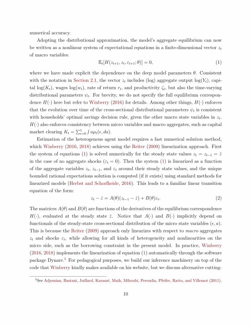
Figure 2: Posterior densities with (blue solid curves) and without (black dashed curves) condition-ing on the micro data. Both sets of results use the same simulated data set. Vertical dashed linesindicate true parameter values. Posterior density estimates from the 9,000 retained MCMC drawsusing Matlab’s ksdensity function with default settings. The third display omits the macro-onlyresults, since µλ is not identified from macro data alone.

which in turn is computed using numerical integration.For simplicity, our MCMC algorithm is a basic Random Walk Metropolis-Hastings algo-

rithm with tuned proposal covariance matrix and adaptive step size (Atchadé and Rosenthal,2005).11 The starting values are determined by a rough grid search on the simulated data.We generate 10,000 draws and discard the first 1,000 as burn-in. Using parallel computingon 20 cores, likelihood evaluation takes about as long as Winberry’s (2016) procedure forcomputing the model’s steady state.

4.3 Results

Figure 2 shows that micro data is useful or even essential for estimating some parameters,but not others. The figure depicts the posterior densities of the three parameters, on a single

11Our proposal distribution is a mixture of (i) the adapted multivariate normal distribution and (ii) adiffuse normal distribution, with 95% probability attached to the former. We verified the DiminishingAdaption condition and Containment condition in Rosenthal (2011), so the distribution of the MCMC drawswill converge to the posterior distribution of the parameters.

19

Heterogeneous household model: Consumption policy function, employed

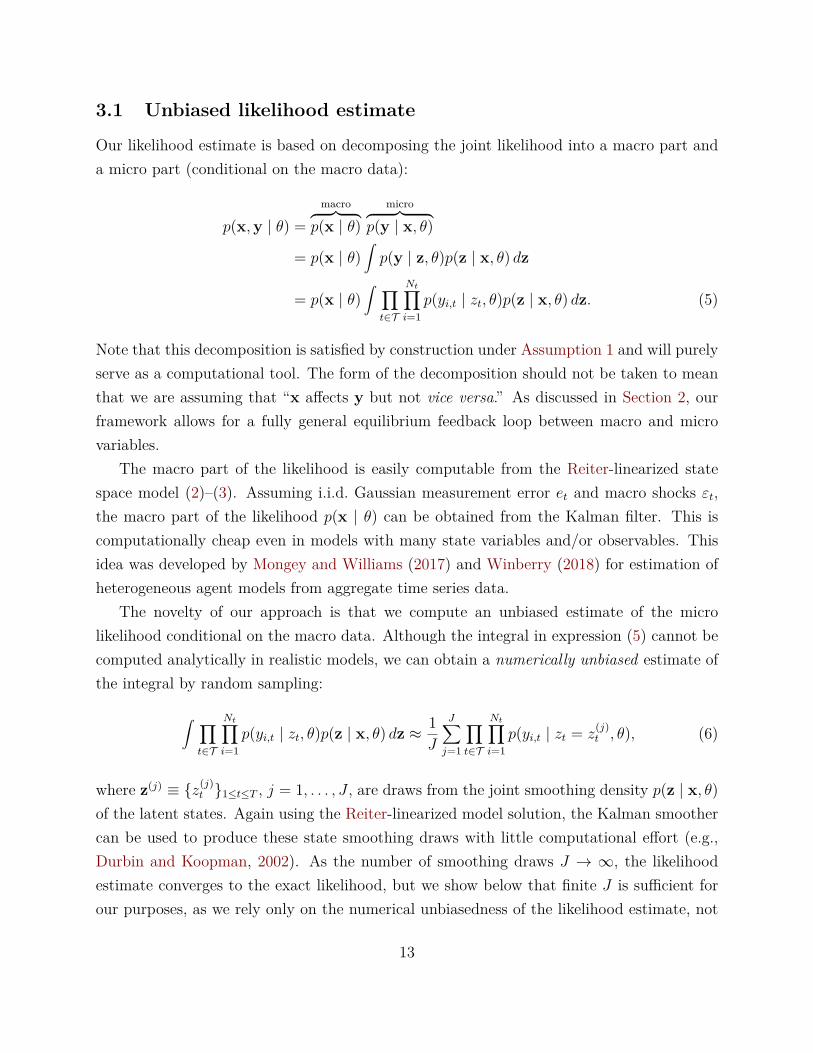
Figure 3: Estimated steady state consumption policy function for employed households, eitherusing both micro and macro data (left panel) or only using macro data (right panel). The thick blackcurve is computed under the true parameters. The thin lines are 900 posterior draws (computedusing every 10th MCMC draw after burn-in). X-axes are normalized asset holdings ai,t.

sample of simulated data. The full-information posterior (blue solid curves) is concentratedclose to the true values of the three parameters (which are marked by vertical thin dashedlines). The figure also shows the posterior density without conditioning on the micro data(black dashed curves). Ignoring the micro data leads to substantially less accurate inferenceabout β in this simulation, as the macro-only posterior is less precisely centered around thetrue value as well as more diffuse than the full-information posterior. Even more starkly,µλ can only be identified from the cross section, since by construction the macro aggregatesare not influenced by the distribution of the individual permanent productivity draws λi. Incontrast, all the information about the measurement error standard deviation σe comes fromthe macro data. Thus, our results here illustrate the general lesson that micro data can beeither essential, useful, or irrelevant for estimating different parameters.

Figure 3 shows that efficient use of the micro data leads to substantially more preciseestimates of the steady state consumption policy function for employed households.12 Theleft panel shows that full-information posterior draws of the consumption policy function

12Figure C.1 in Supplemental Appendix C.2 plots the policy function for unemployed households.

20

Het. household model: Impulse responses of asset distribution, employed

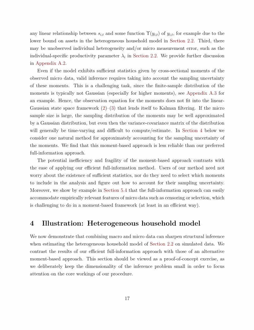
Figure 4: Estimated impulse response function of employed households’ asset distribution withrespect to an aggregate productivity shock, either using both micro and macro data (left panel)or only using macro data (right panel). The thin lines are 900 posterior draws (computed usingevery 10th MCMC draw after burn-in). X-axes are normalized asset holdings ai,t. The four rows ineach panel are the asset densities at impulse response horizons 0 (impact), 2, 4, and 8. The blackdashed and black solid curves are the steady state density and the impulse response, respectively,computed under the true parameters. On impact the true impulse response equals the steady statedensity, since households’ portfolio choice is predetermined.

(thin curves) are fairly well centered around the true function (thick curve), as is expectedgiven the accurate inference about β depicted in Figure 2. In contrast, the right panelshows that macro-only posterior draws are less well centered and exhibit higher variance,especially for households with high or low current asset holdings. The added precisionafforded by efficient use of the micro data translates into more precise estimates of themarginal propensity to consume (the derivative of the consumption policy function) at theextremes of the asset distribution. This is potentially useful when analyzing the two-wayfeedback effect between macroeconomic policies and redistribution (Auclert, 2019).

The extra precision afforded by micro data also sharpens inference on the impulse re-sponse function of the asset distribution with respect to an aggregate productivity shock.Figure 4 shows full-information (left panel) and macro-only (right panel) posterior draws ofthe impulse response function of employed households’ asset holding density, in the periods

21

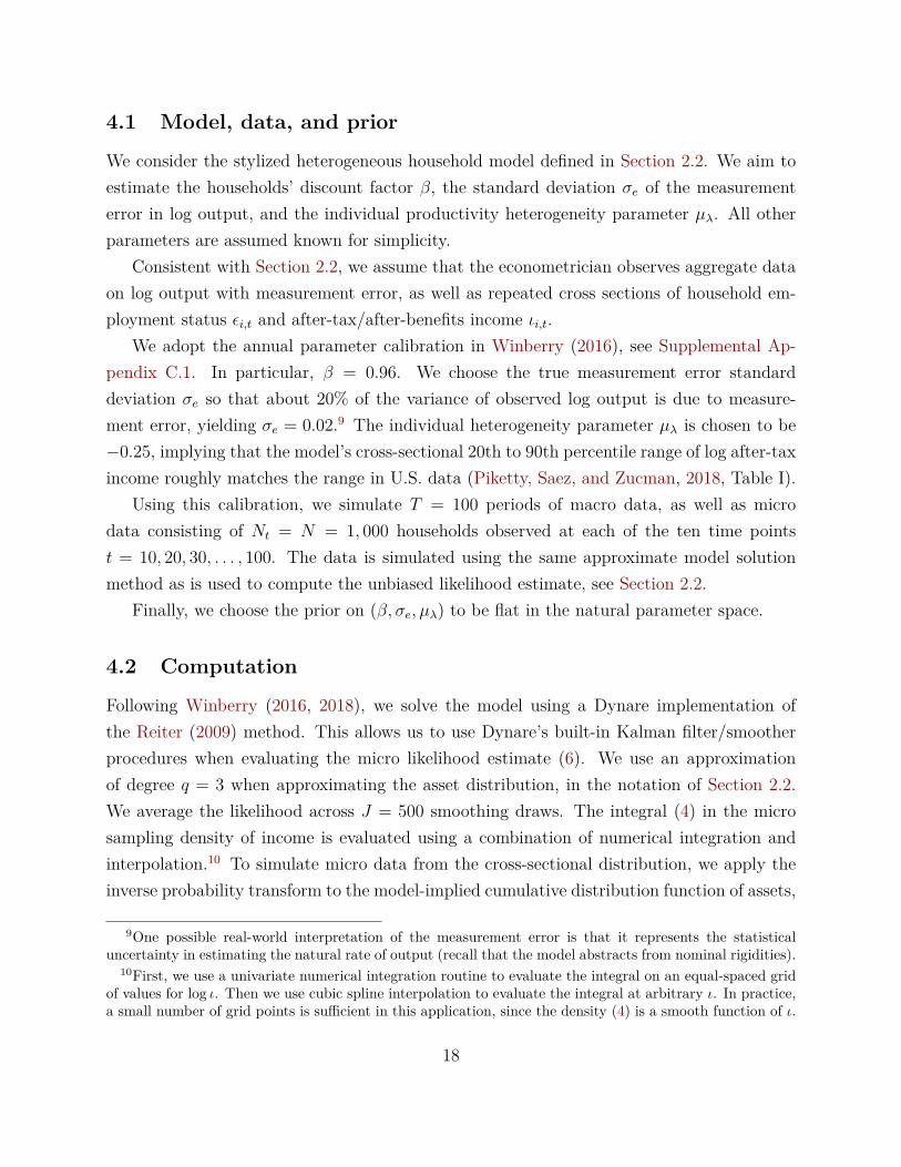
Heterogeneous household model: Posterior density, multiple simulations

Figure 5: Posterior densities with (blue curves) and without (gray curves) conditioning on themicro data, for 10 different simulated data sets. See also caption for Figure 2.

following a 5% aggregate productivity shock.13 Once again, the full-information results havesubstantially lower variance. Following the shock, there is a noticeable movement of the as-set distribution computed under the true parameters (black solid curve). At horizon h = 8,the mean increases by 0.16 relative to the steady state (black dashed curve), the varianceincreases by 0.10, and the third central moment decreases by 0.06. However, the true move-ment in the asset distribution is not so large relative to the estimation uncertainty. Thisfurther motivates the use of an efficient inference method that validly takes into account allestimation uncertainty.

The previous qualitative conclusions hold up in repeated simulations from the calibratedmodel. We repeat the MCMC estimation exercise on 10 different simulated data sets.14 Fig-ure 5 plots all 10 full-information and macro-only posterior densities for the three parameterson the same plot. Notice that the full-information densities for β systematically concentratecloser to the true value than the macro-only posteriors do, as in Figure 2.

Our inference approach is valid in the usual Bayesian sense no matter how small the

13For unemployed households, see Figure C.2 in Supplemental Appendix C.2.14Computational constraints preclude a full Monte Carlo study.

22

sample size is. In Figure C.3 of Supplemental Appendix C.2 we show that the full-informationapproach still yields useful inference about the model parameters if we only observe N = 100observations every ten periods (instead of N = 1000 as above).

4.4 Comparison with moment-based methods

In this subsection, we compare the above full-information results with a moment-based in-ference approach, to shed light on the theoretical comparison in Section 3.3. Due to theunobserved individual heterogeneity parameter λi, fixed-dimensional sufficient statistics donot exist in this model with the given observables.15 Hence, we follow empirical practiceand compute an ad hoc selection of cross-sectional moments, including the sample mean,variance, and third central moment of household after-tax income. We compute the mo-ments separately for the groups of employed and unemployed households, in each periodt = 10, 20, . . . , 100 where micro data is observed. We consider three moment-based ap-proaches with different numbers of observables: The “1st Moment” approach only incorpo-rates time-series of sample means, the “2nd Moment” approach incorporates both samplemeans and variances, and the “3rd Moment” approach incorporates sample moments up tothe third order.

Once we compute the time series of cross-sectional moments on the simulated data, wetreat them as additional time series observables and proceed as in the “Macro Only” approachconsidered earlier. To account for the sampling uncertainty in the cross-sectional moments,we appeal to a Central Limit Theorem and treat the moments as jointly Gaussian, whichis equivalent to adding measurement error in those state space equations that correspondto the moments. A natural and practical way to construct the variance-covariance matrixof the measurement error is to estimate its elements using higher-order sample momentsof micro data. The variance-covariance matrix is actually time-varying according to thestructural model, but since this would be challenging to account for, we treat it as fixedover the sample.16 Supplemental Appendix B provides the details of how we estimate thevariance-covariance matrix. The computation time of the moment-based likelihood functionsis comparable to our full-information approach, since most of the time is taken up by the

15The unobserved individual heterogeneity is observationally equivalent to micro measurement error givenrepeated cross sections of micro data.

16Higher-order sample moments are less accurate approximations to their population counterparts. Givenan empirically relevant cross-sectional sample size, the resulting variance-covariance matrix would be evenmore imprecise if inferred period by period.

23

Heterogeneous household model: Likelihood comparison

0.95 0.96 0.97 0.98-10

-8

-6

-4

-2

0

1st Moment 2nd Moment 3rd Moment Macro Only Full Info

0.02 0.04 0.06 0.08-10

-8

-6

-4

-2

0e

-0.32 -0.3 -0.28 -0.26 -0.24-10

-8

-6

-4

-2

0

Figure 6: Comparison of log likelihoods across inference methods, based on one typical simulateddata set. Each panel depicts univariate deviations of a single parameter while keeping all otherparameters at their true values. The maximum of each likelihood curve is normalized to be zero.Vertical dashed lines indicate true parameter values. The “1st Moment” and “Macro Only” curvesare flat on the right panel, since µλ is not identified from this data alone. For results across 10different simulated data sets, see Figure 9 in Appendix A.4.

calculation of the model’s steady state (which is common to all methods).We compare the shape and location of the likelihood functions for the full-information

and moment-based methods.17 For graphical clarity, we vary a single parameter at a time,keeping the other parameters at their true values. Figure 6 plots the univariate log likelihoodsfunctions of all inference approaches based on one typical simulated data set.18 Since we areinterested in the curvature of the likelihood functions near their maxima, and not the overalllevel of the functions, we normalize each curve by subtracting its maximum.

Figure 6 shows that the moment-based likelihoods do not approximate the efficient full-information likelihood well, with the “3rd Moment” likelihood being particularly inaccuratelycentered. There are two reasons for this. First, as discussed in Section 3.3, there is no the-

17We omit full posterior inference results for the moment-based methods, as they were more prone toMCMC convergence issues than our full-information method.

18We compute the full-information likelihood function by averaging across J = 500 smoothing draws. Fora clearer comparison of the plotted likelihood functions, we fix the random numbers used to draw fromthe smoothing distribution across parameter values. Note that we do not fix these random numbers in theMCMC algorithm, as required by the Andrieu, Doucet, and Holenstein (2010) argument.

24

oretical sufficient statistics in this setup, so all the moment-based approaches incur someefficiency loss. Second, the sampling distributions of higher-order sample moments are notwell approximated by Gaussian distributions in finite samples, and the measurement errorvariance-covariance matrix depends on even higher-order moments, which are poorly esti-mated. A separate issue is that the individual heterogeneity parameter µλ cannot evenbe identified using the “1st Moment” approach, since this parameter does not influencefirst moments of the micro data. The “2nd Moment” likelihood is not entirely mislead-ing but nevertheless differs meaningfully from the full-information likelihood.19 Figure 9 inAppendix A.4 confirms that the aforementioned qualitative conclusions hold up across 10different simulated data sets.

To summarize, even in this relatively simple model, the moment-based methods we con-sider lead to a poor approximation of the full-information likelihood, and the inference canbe highly sensitive to the choice of which moments to include. It is possible that other im-plementations of the moment-based approach would work better in particular applications.Nevertheless, any moment-based approach will require challenging ad hoc choices, such aswhich moments to use and how to account for their sampling uncertainty. No such choicesare required by the efficient full-information approach developed in this paper.

5 Illustration: Heterogeneous firm model

As our second proof-of-concept example, we estimate a version of the heterogeneous firmmodel of Khan and Thomas (2008). In addition to showing that our general inference ap-proach can be applied outside the specific Krusell and Smith (1998) family of models, we usethis section to illustrate how sample selection or data censoring can easily be accommodatedin our method.

5.1 Model, data, and prior

A continuum of heterogeneous firms are subject to both idiosyncratic and aggregate produc-tivity shocks. Firms must pay a fixed cost whenever their investment, as a fraction of their

19The “Full Info” and “Macro Only” likelihoods are consistent with the posterior densities plotted inSection 4.3. For β, the “Macro Only” likelihood has a smaller curvature around the peak and a wider rangeof peaks across simulated data sets, so the full information method helps sharpen the inference of β. For σe,the “Macro Only” curves are close to their “Full Info” counterparts. The parameter µλ is not identified inthe “Macro Only” case, so the corresponding likelihood function is flat.

25

existing capital stock, exceeds a certain magnitude. In addition to the aggregate productivityshock, there is a second aggregate shock that affects investment efficiency. The representativehousehold has additively separable preferences over log consumption and (close to linear)leisure time. For brevity, we relegate the details of the model to Supplemental Appendix D.1,which entirely follows Winberry’s (2018) version of the Khan and Thomas (2008) model.

We aim to estimate the AR(1) parameter ρε and innovation standard deviation σε of thefirms’ idiosyncratic log productivity process. Khan and Thomas (2008) showed that theseparameters have little impact on the aggregate macro implications of the model; hence, microdata is needed. All other structural parameters are assumed known for simplicity.

We adopt the annual calibration of Winberry (2018), which in turn follows Khan andThomas (2008), see Supplemental Appendix D.2. However, we make an exception in settingthe true idiosyncratic AR(1) parameter ρε = 0.53, following footnote 5 in Khan and Thomas(2008).20 We then set σε = 0.0364, so that the variance of the idiosyncratic log productivityprocess is unchanged from the baseline calibration in Khan and Thomas (2008) and Winberry(2018). The macro implications of our calibration are virtually identical to the baseline inKhan and Thomas (2008), as those authors note.

We assume that the econometrician observes time series on aggregate output and invest-ment, as well as repeated cross sections of micro data on firms’ capital and labor inputs. Wesimulate macro data with sample size T = 50, while micro cross sections of size N = 1000are observed at each of the five time points t = 10, 20, . . . , 50. Unlike in Section 4, we do notadd measurement error to the macro observables.

The prior on (ρε, σε) is chosen to be flat in the natural parameter space.

5.2 Computation

As in Section 4, we solve and simulate the model using the Winberry (2018) Dynare solutionmethod. We follow Winberry (2018) and approximate the cross-sectional density of the firms’micro state variables (log capital and idiosyncratic productivity) with a multivariate normaldistribution. Computation of the micro sampling density is simple, since – conditional onmacro states – the micro observables (capital and labor) are log-linear transformations ofthese micro state variables. We use J = 500 smoothing draws to compute the unbiasedlikelihood estimate. The MCMC routine is the same as in Section 4. The starting valuesare selected by a rough grid search on the simulated data. We generate 10,000 draws and

20This avoids numerical issues that arise when solving the model for high degrees of persistence.

26

discard the first 1,000 as burn-in. Likelihood evaluation using 20 parallel cores is severaltimes faster than computing the model’s steady state.

5.3 Results

Despite the finding in Khan and Thomas (2008) that macro data is essentially uninformativeabout the idiosyncratic productivity parameters, these are accurately estimated when themicro data is used also. Figure 7 shows the posterior densities of ρε and σε computedon several different simulated data sets.21 The posterior distribution of each parameter issystematically concentrated close to the true parameter values. We refrain from visuallycomparing these results with inference that relies only on macro data, since the macrolikelihood is almost entirely flat as a function of (ρε, σε), consistent with Khan and Thomas(2008).22 Thus, micro data is essential to inference about these parameters.

5.4 Correcting for imperfect sampling of micro data

One advantage of the likelihood approach adopted in this paper is that standard techniquescan be applied to correct for sample selection or censoring in the micro data. This is highlyrelevant for applied work, since household or firm surveys are often subject to known dataimperfections, even beyond measurement error.

Valid inference about structural parameters merely requires that the micro samplingdensity p(yi,t | zt, θ) introduced in Section 2.1 accurately reflects the sampling mechanism,including the effects of selection or censoring. Hence, if it is known, say, that an observedvariable such as household income is top-coded (i.e., censored) at the threshold y, then thefunctional form of the density p(yi,t | zt, θ) should take into account that the observed dataequals a transformation yi,t = min{yi,t, y} of the theoretical household income yi,t in theDSGE model. The likelihood functions of such limited dependent variable sampling modelsare well known and readily looked up, see for example Wooldridge (2010, chapters 17 and19).23 We provide one illustration below.

21We show results for 9 rather than 10 different simulations, since the MCMC chain did not mix well onone of the simulations.

22On average across the 9 simulated data sets, the standard deviation (after burn-in) of the macro loglikelihood across all Metropolis-Hastings proposals of the parameters is only 0.12, while it is 11.0 for themicro log likelihood.

23If the nature of the data imperfection is only partially known, it may be possible to estimate the samplingmechanism from the data. For example, if the data is suspected to be subject to endogenous sample selection,

27

Heterogeneous firm model: Posterior density, multiple simulations

Figure 7: Posterior densities across 9 simulated data sets. Vertical dashed lines indicate trueparameter values. Posterior density estimates from the 9,000 retained MCMC draws using Matlab’sksdensity function with default settings.

Other approaches to estimating heterogeneous agent models do not handle data imper-fections as easily or efficiently. For example, inference based on cross-sectional momentsof micro observables may require lengthy derivations to adjust the moment formulas forselection or censoring, especially for higher moments. Moreover, even in models where low-dimensional sufficient statistics exist for the underlying micro variables, cf. Section 3.3, theimperfectly observed micro data may not afford such sufficient statistics. In contrast, ourlikelihood-based approach is automatically efficient, and the adjustments needed to accountfor common types of data imperfections can be looked up in microeconometrics textbooks.

Illustration: Selection on outcomes. We illustrate the previous points by addingan endogenous selection mechanism to the sampled micro data in the heterogeneous firmmodel. Assume that instead of observing a representative sample of N = 1000 firms everyten periods, we only observe the draws for those firms whose employment in that period

one could specify a Heckman-type selection model and estimate the parameters of the selection model as partof the likelihood framework (Wooldridge, 2010, chapter 19). It is outside the scope of this paper to considernonparametric approaches or to analyze the consequences of misspecification of the sampling mechanism.

28

exceeds the 90th percentile of the steady-state cross-sectional distribution of employment.That is, out of 1000 potential draws in a period, we only observe the capital and laborinputs of the approximately 100 largest firms. Though stylized, this sampling mechanismis intended to mimic the real-world phenomenon that databases such as Compustat tend toonly cover the largest active firms in the economy.

To adjust the likelihood for selection, we combine the model-implied cross-sectional dis-tribution of the idiosyncratic state variables with the functional form of the selection mech-anism. Let gt(ε, k) be the cross-sectional distribution of idiosyncratic log productivity εi,t

and log capital ki,t at time t, implied by the model (this density is approximated using anexponential family of densities, as in Winberry, 2018). In the model, log employment isgiven by ni,t = (log ν + ζt − log(wt) + εi,t + αki,t)/(1 − ν), where wt is the aggregate wage,ζt is log aggregate TFP, and ν and α are the output elasticities of labor and capital in thefirm production function (ν+α < 1). Since observations yi,t = (ni,t, ki,t)′ are observed if andonly if ni,t ≥ n, the micro sampling density is given by the truncation formula24

p(ni,t, ki,t | zt, θ) =(1− ν)gt

((1− ν)ni,t − αki,t − log ν − ζt + log(wt), ki,t

)∫∞−∞

∫∞−∞ 1

(log ν + ζt − log(wt) + ε+ αk ≥ (1− ν)n

)gt(ε, k) dε dk

.

The selection threshold n is given by the true 90th percentile of the steady-state distributionof log employment. We assume this threshold is known to the econometrician for simplicity.25

Figure 8 shows the posterior distribution of the idiosyncratic productivity AR(1) pa-rameters (ρε, σε) in the model with selection. All settings are the same as in Section 5.1,except for the selection mechanism in the simulated micro data and the requisite adjustmentto the functional form of the micro likelihood function. The posterior distributions of theparameters of interest remain centered close to the true parameter values. The posteriordensity is inevitably less tightly concentrated around the true values than in Figure 7 be-cause the effective micro sample size is now smaller by a factor of approximately 10 due toselection. Still, the example demonstrates that data imperfections can be handled in a validand efficient manner using standard likelihood techniques.

24The integral in the denominator can be computed in closed form if the density gt(ε, k) is multivariateGaussian, which is the approximation we use in our numerical experiments, following Winberry (2018).

25In principle, n could be treated as another parameter to be estimated from the available data.

29

Heterogeneous firm model: Posterior density with selection

0.45 0.5 0.55 0.6

0

5

10

15

20

0.03 0.035 0.04

0

100

200

300

400

Figure 8: Posterior densities in a simulated data set with selection. Vertical dashed lines indicatetrue parameter values. Posterior density estimates from the 9,000 retained MCMC draws usingMatlab’s ksdensity function with default settings.

6 Conclusion

The literature on heterogeneous agent models has hitherto relied on estimation approachesthat exploit ad hoc choices of micro moments and macro time series for estimation. Thiscontrasts with the well-developed framework for full-information likelihood inference in rep-resentative agent models (Herbst and Schorfheide, 2016). We develop a method to exploitthe full information content in macro and micro data when estimating heterogeneous agentmodels. As we demonstrate through economic examples, the joint information content avail-able in micro and macro data is often much larger than in either of the two separate datasets. Our inference procedure can loosely be interpreted as a two-step method: First weestimate the underlying macro states from macro data, and then we evaluate the likelihoodby plugging into the cross-sectional sampling densities given the estimated states. However,our method delivers finite-sample valid and fully efficient Bayesian inference that takes intoaccount all sources of uncertainty about parameters and states. The computation time of ourprocedure scales well with the size of the data set, as the method lends itself to parallel com-puting. Unlike estimation approaches based on tracking a small number of cross-sectionalmoments over time, our full-information method is automatically efficient and can easily ac-commodate unobserved individual heterogeneity, micro measurement error, as well as data

30

imperfections such as censoring or selection.For clarity, we have limited ourselves to numerical illustrations with small-scale models in

this paper, leaving full-scale empirical applications to future work. Our approach is compu-tationally most attractive when the model is solved using some version of the Reiter (2009)linearization approach, since this yields simple formulas for evaluating the macro likelihoodand drawing from the smoothing distribution of the latent macro states, cf. Section 3. Toestimate large-scale quantitative models it would be necessary to apply now-standard dimen-sion reduction techniques to the linearized macro state space representation (Ahn, Kaplan,Moll, Winberry, and Wolf, 2017), and we leave this to future research. Our method alsofits best with model solution methods that work in the state space rather than the sequencespace (Auclert, Bardóczy, Rognlie, and Straub, 2020), as the former yields immediate for-mulas for the micro sampling density conditional on the macro states. Nevertheless, weemphasize that our method is in principle generally applicable, as long as there exists someway to evaluate the macro likelihood, draw from the smoothing distribution of the macrostates, and evaluate the micro sampling density given the macro states.

Our research suggests several additional avenues for future research. First, it would beinteresting to extend our method to allow for panel data. Unlike in the case of repeated crosssections, panel data complicates the evaluation of the micro likelihood due to the intricateserial dependence of individual decisions. Second, since our method works for a wide rangeof generic MCMC posterior sampling procedures, it would be interesting to investigate thescope for improving on the simple Random Walk Metropolis-Hastings algorithm that we usefor conceptual clarity in our examples. Third, the goal of this paper has been to fully exploitall aspects of the assumed heterogeneous agent model when doing statistical inference; wetherefore ignore the consequences of misspecification. Since model misspecification poten-tially affects the entire macro equilibrium and thus cannot be addressed using off-the-shelftools from the microeconometrics literature, we leave the development of robust inferenceapproaches to future work.

31

A Appendix

A.1 Proofs

A.1.1 Proof of Theorem 1

Let mt ≡ (m1,t, . . . , mQ,t)′ denote the set of sufficient statistics in period t. According to theFisher-Neyman factorization theorem, there exists a function h(·) such that the likelihoodof the micro data in period t, conditional on zt, can be factorized as

Nt∏i=1

p(yi,t | zt, θ) = h(yt)p(mt | Nt, zt, θ). (10)

Let h(y) = ∏t∈T h(yt), N = {Nt}t∈T , and m = {mt}t∈T , where T is the subset of time

points with observed micro data. Then the micro likelihood, conditional on the observedmacro data, can be decomposed as

p(y | x, θ) =∫p(y | z, θ)p(z | x, θ) dz

= h(y)∫p(m | N, z, θ)p(z | x, θ) dz (11)

= h(y)p(m | N,x, θ). (12)

The expression (12) implies that m is a set of sufficient statistics for θ, based again on theFisher-Neyman factorization theorem.

A.1.2 Proof of Corollary 1

Let mt be a vector of population counterparts of the cross-sectional sufficient statistics ofthe micro states si,t. We may view mt as part of the macro state vector zt. According to theexponential polynomial setup,

p(si,t | zt, θ) = p(si,t | mt)

= expϕ0(mt) +

Q∑`=1

ϕ`(mt)m`(si,t) .

m`(si,t) takes the form sp1i,t,1s

p2i,t,2 · · · s

pdsi,t,ds

with pk being positive integers and 1 ≤ ∑dsk=1 pk ≤ q,

where q is the order of the exponential polynomial. The potential number of sufficient statis-

32

tics Q equals(q+ds

q

)− 1, i.e., the number of complete homogeneous symmetric polynomials.

Making the change of variables in (9), we have

p(yi,t | zt, θ) = expϕ0(mt) +

Q∑`=1

ϕ`(mt)m`

(B1(zt, θ)Υ(yi,t) +B0(zt, θ)

)×∣∣∣∣∣det

(B1(zt, θ)

∂Υ(yi,t)∂yi,t

)∣∣∣∣∣≡ exp

ϕ0(zt, θ) + m0(yi,t) +Q∑`=1

ϕ`(zt, θ)m`(yi,t) .

Given assumptions 2.a and 2.b, the potential number of sufficient statistics Q remains thesame. Now the sufficient statistics can be expressed as m`(yi,t) ≡ m`(Υ(yi,t)) and the corre-sponding ϕ`(zt, θ) can be obtained by rearranging terms and collecting coefficients on m`(yi,t).For the determinant of the Jacobian, condition 2 implies that both B1(zt, θ) and ∂Υ(yi,t)

∂yi,tare

non-singular square matrices, so det(B1(zt, θ)∂Υ(yi,t)

∂yi,t

)= det (B1(zt, θ)) det

(∂Υ(yi,t)∂yi,t

). Hence,

both log |det (B1(zt, θ))| and log∣∣∣det

(∂Υ(yi,t)∂yi,t

)∣∣∣ are finite and can be absorbed into ϕ0(zt, θ)and m0(yi,t), respectively.

Thus, the micro likelihood fits into the general form in Theorem 1, and the sufficientstatistics are given by

m`,t = 1Nt

Nt∑i=1

m`(yi,t) = 1Nt

Nt∑i=1

m`(Υ(yi,t)), ` = 1, . . . , Q.

A.2 Non-existence of sufficient statistics: Details

Can we generalize beyond the sufficient conditions in Corollary 1? The key is that in (7),the terms inside the exponential should be additive and each term should take the formϕ`(zt, θ)m`(yi,t), which ensures that the cross-sectional moments can be calculated usingmicro data as in equation (8) and the multiplicative term h(y) can be taken out of theintegral in equation (11). Building on the analysis of Section 3.3, here are more detailsregarding cases where there are no sufficient statistics in general.

i) si,t = B1(zt, θ)Υ(yi,t, zt) +B0(zt, θ), i.e., yi,t and zt are neither additively nor multiplica-tively separable.

ii) The model features unobserved individual heterogeneity and/or micro measurement er-ror. Since these two cases are observationally equivalent in a repeated cross section

33

framework, we focus on the the former. Letting λi denote the unobserved individualheterogeneity, we can extend (9) to si,t = Υ(yi,t, λi, zt, θ) ≡ B1(λi, zt, θ)Υ(yi,t, λi) +B0(λi, zt, θ), which is the most general setup allowing λi to affect all terms in the ex-pression. If λi is independent of si,t conditional on (zt, θ), we have p(si,t, λi | zt, θ) =p(si,t | mt)p(λi | θ) (recall the notation in the proof of Corollary 1). Accordingly,

p(yi,t | zt, θ) =∫p(Υ(yi,t, λi, zt, θ) | mt)

∣∣∣∣∣det(B1(λi, zt, θ)

∂Υ(yi,t, λi)∂yi,t

)∣∣∣∣∣ p(λi | θ) dλi.If λi appears in B1, B0, or Υ, then p(yi,t | zt, θ) may not belong to the exponentialfamily after integrating out λi. That said, we can construct special cases where sufficientstatistics do exist. For example, if si,t = B1(zt, θ)Υ(yi,t) + B0(zt, θ) + B2(zt, θ)λi andboth p(si,t | mt) and p(λi | θ) follow Gaussian distributions.

iii) ds > dy: For example, suppose si,t is two-dimensional whereas yi,t is one-dimensional,say yi,t = s1,i,t, yi,t = s1,i,t + s2,i,t, or yi,t = s1,i,ts2,i,t. We can first expand the yi,t in(9) to yi,t = (yi,t, s2,i,t)′ and then integrate out s2,i,t. However, after the integration, theresulting micro likelihood as a function of yi,t may not take the exponential family formanymore.

A.3 Sampling distribution of cross-sectional moments: Example

As alluded to in Section 3.3, here is a simple example demonstrating that p(mt | Nt, zt, θ)is not linear Gaussian in finite samples, and therefore neither is p(m | N,x, θ). Supposeyi,t = si,t is a scalar and p(si,t | mt) is Gaussian, i.e., a second-order exponential polynomial.Let m1,t = 1

Nt

∑Nti=1 si,t and m2,t = 1

Nt

∑Nti=1(si,t − m1,t)2 with m1,t and m2,t being their

population counterparts. Then standard calculations yield

p(mt | Nt, zt, θ) = p(mt | mt) = φ(m1,t; m1,t,

m2,t

Nt

)pχ2

(Ntm2,t

m2,t; Nt − 1

),

where φ(x;µ, σ2) represents the probability distribution function (pdf) of a Gaussian distri-bution with mean µ and variance σ2, and pχ2(x; ν) is the pdf of a chi-squared distributionwith ν degrees of freedom. We can see that the latter is not linear Gaussian. Moreover,when p(si,t | mt) follows a higher order exponential polynomial, the characterization ofp(mt | Nt, zt, θ) would be even more complicated without a closed-form expression.

34

A.4 Heterogeneous household model: Likelihood comparison

Complementing the results for a single simulated data set in Section 4.4, Figure 9 compareslog likelihoods for the different inference methods across 10 different simulated data sets.Here different inference methods are exhibited in different rows. Similar to Figure 6, eachcolumn depicts univariate deviations of a single parameter while keeping all other parametersat their true values. There are 10 likelihood curves in each panel, corresponding to the 10simulated data sets. The maximum of each likelihood curve is normalized to be zero. Verticaldashed lines indicate true parameter values. The “1st Moment” and “Macro Only” curvesare flat on the right panels of the second and the last rows, since µλ is not identified from thisdata alone. We conclude from the figure that the full-information likelihood is systematicallywell-centered and tightly concentrated around the true parameter values, whereas the variousmoment-based likelihoods are poorly centered, exhibit less curvature, and/or shift aroundsubstantially across simulations.

35

Het. household model: Likelihood comparison, multiple simulations

β σe µλ

FullInfo

Macro

Only

3rdMom

ent

2ndMom

ent

1stMom

ent

Figure 9: Comparison of log likelihood functions across 10 different simulated data sets. See thedescription in Appendix A.4.

36

References

Acharya, S., M. D. Negro, and K. Dogra (2020): “Estimating HANK: Macro TimeSeries and Micro Moments,” Paper presented at the 2021 North American Winter Meetingof the Econometric Society.

Adjemian, S., H. Bastani, M. Juillard, F. Karamé, J. Maih, F. Mihoubi,G. Perendia, J. Pfeifer, M. Ratto, and S. Villemot (2011): “Dynare: Refer-ence Manual Version 4,” Dynare Working Papers 1, CEPREMAP.

Ahn, S., G. Kaplan, B. Moll, T. Winberry, and C. Wolf (2017): “When InequalityMatters for Macro and Macro Matters for Inequality,” in NBER Macroeconomics Annual,Volume 32, ed. by J. A. Parker, and M. Woodford, pp. 1–75. University of Chicago Press.

Andrieu, C., A. Doucet, and R. Holenstein (2010): “Particle Markov chain MonteCarlo methods,” Journal of the Royal Statistical Society: Series B, 72(3), 269–342.

Arellano, M., and S. Bonhomme (2017): “Nonlinear Panel Data Methods for DynamicHeterogeneous Agent Models,” Annual Review of Economics, 9(1), 471–496.

Atchadé, Y. F., and J. S. Rosenthal (2005): “On adaptive Markov chain Monte Carloalgorithms,” Bernoulli, 11(5), 815–828.

Auclert, A. (2019): “Monetary Policy and the Redistribution Channel,” American Eco-nomic Review, 109(6), 2333–2367.

Auclert, A., B. Bardóczy, M. Rognlie, and L. Straub (2020): “Using the Sequence-Space Jacobian to Solve and Estimate Heterogeneous-Agent Models,” Manuscript, Stan-ford University.

Auclert, A., M. Rognlie, and L. Straub (2020): “Micro Jumps, Macro Humps: Mon-etary Policy and Business Cycles in an Estimated HANK Model,” Manuscript, StanfordUniversity.

Bayer, C., B. Born, and R. Luetticke (2020): “Shocks, Frictions, and Inequality inUS Business Cycles,” CEPR Discussion Paper 14364.

Challe, E., J. Matheron, X. Ragot, and J. F. Rubio-Ramirez (2017): “Precau-tionary saving and aggregate demand,” Quantitative Economics, 8(2), 435–478.

37

Chang, M., X. Chen, and F. Schorfheide (2018): “Heterogeneity and Aggregate Fluc-tuations,” Manuscript, University of Pennsylvania.

Chang, Y., J. F. Gomes, and F. Schorfheide (2002): “Learning-by-Doing as a Prop-agation Mechanism,” American Economic Review, 92(5), 1498–1520.

Durbin, J., and S. J. Koopman (2002): “A simple and efficient simulation smoother forstate space time series analysis,” Biometrika, 89(3), 603–616.

Fernández-Villaverde, J., S. Hurtado, and G. Nuño (2018): “Financial Frictionsand the Wealth Distribution,” Manuscript, University of Pennsylvania.

Flury, T., and N. Shephard (2011): “Bayesian Inference Based Only on SimulatedLikelihood: Particle Filter Analysis of Dynamic Economic Models,” Econometric Theory,27(05), 933–956.

Hahn, J., G. Kuersteiner, and M. Mazzocco (2018): “Central Limit Theory forCombined Cross-Section and Time Series,” Manuscript, arXiv:1610.01697.

Hasumi, R., and H. Iiboshi (2019): “A Bayesian Estimation of HANK models with Con-tinuous Time Approach: Comparison between US and Japan,” Munich Personal RePEcArchive Paper No. 92292.

Herbst, E., and F. Schorfheide (2016): Bayesian Estimation of DSGE Models, Econo-metric and Tinbergen Institutes Lectures. Princeton University Press.

Kaplan, G., and G. L. Violante (2018): “Microeconomic Heterogeneity and Macroeco-nomic Shocks,” Journal of Economic Perspectives, 32(3), 167–194.

Khan, A., and J. K. Thomas (2008): “Idiosyncratic Shocks and the Role of Nonconvex-ities in Plant and Aggregate Investment Dynamics,” Econometrica, 76(2), 395–436.

Krueger, D., K. Mitman, and F. Perri (2016): “Macroeconomics and Household Het-erogeneity,” in Handbook of Macroeconomics, Volume 2, ed. by J. B. Taylor, and H. Uhlig,chap. 11, pp. 843–921. Elsevier.

Krueger, D., F. Perri, L. Pistaferri, and G. L. Violante (2010): “Cross-sectionalfacts for macroeconomists,” Review of Economic Dynamics, 13(1), 1–14.

38

Krusell, P., and A. A. Smith (1998): “Income and Wealth Heterogeneity in the Macroe-conomy,” Journal of Political Economy, 106(5), 867–896.

Mongey, S., and J. Williams (2017): “Firm dispersion and business cycles: Estimatingaggregate shocks using panel data,” Manuscript, New York University.

Papp, T. K., and M. Reiter (2020): “Estimating linearized heterogeneous agent modelsusing panel data,” Journal of Economic Dynamics and Control, 115, 1–17.

Parra-Alvarez, J. C., O. Posch, and M.-C. Wang (2020): “Estimation of heteroge-neous agent models: A likelihood approach,” CREATES Research Paper 2020-05.

Piketty, T., E. Saez, and G. Zucman (2018): “Distributional National Accounts: Meth-ods and Estimates for the United States,” Quarterly Journal of Economics, 133(2), 553–609.

Reiter, M. (2009): “Solving Heterogeneous-Agent Models by Projection and Perturba-tion,” Journal of Economic Dynamics and Control, 33(3), 649–665.

Rosenthal, J. S. (2011): “Optimal proposal distributions and adaptive MCMC,” Hand-book of Markov Chain Monte Carlo, 4(10.1201).

Winberry, T. (2016): “User Guide for “A Toolbox for Solving and Estimating Heteroge-neous Agent Macro Models”,” Manuscript, University of Chicago Booth School of Business.

(2018): “A method for solving and estimating heterogeneous agent macro models,”Quantitative Economics, 9(3), 1123–1151.

Wolff, E. N. (2016): “Household Wealth Trends in the United States, 1962 to 2013: WhatHappened over the Great Recession?,” RSF: The Russell Sage Foundation Journal of theSocial Sciences, 2(6), 24–43.

Wooldridge, J. (2010): Econometric Analysis of Cross Section and Panel Data. MITPress, 2nd edn.

39