A BASIC APPROACH TO THE EVALUATION OF .

RISKY INTERRELATED INVESTMENTS

by

Frederick S. Hillier*

TECHNICAL REPORT NO. 69-9

August 15, 1969

OPERATIONS RESEARCH HOUSESTANFORD UNIVERSITYSTANFORD, CALIFORNIA

This research was supported in part by the Office of NavalResearch Contracts Nonr-225(89)(NR-047061) and Nonr-225(53)(NR-042-002) and National Science Foundation Grant GP-7074.

Research and repruduction of this report was partially supported byOffice of Naval Research, Contract3 ONR-N-00014-67-A-0112-0011 andONR-N-00014-67-A-0112-0016; U.S. Atomic Energy Commission, ContractAT[04-33-326 PA #18; National Science Foundation Grant GP-6431;U.S. Army Research Office, Contract DAHC04-67-CO028; and NationalInstitute of Health, Grant GM 14789-02.

Reproduction in whole or in part is permitted for any purpose of theUnited States Government. This document has been approved for publicrelease and sale; its distribution is unlimited.

A BASIC APPROACH TO THE EVALUATION OF

RISKY INMERIATED IIIVESTNTS

byFrederick S. Hillier

1. Introduction

When evaluating proposals for capital investment, it often is

necessary to consider interrelationsh.ps of various kinds between the

projects. For example, some projects may be complementary, such as

those which would benefit in common from the facilities that would

need to be provided for any one of them. Some proposals may even be

necessarily contingent on undertaking one or more prerequisite projects

or on the occurrence of particular favorable conditions. Certain

proposals may instead be mutually exclusive in that they involve

different ways of performing the same service. Other proposed invest-

ments may at least be competitive in the sense that undertaking one

reduces the benefits that would result from also undertaking any of

the others. Furthermore, some or all of the proposals may need to

compete for certain limited resources such as capital, manpower, and

facilities.

Fortunately, considerable progress has been made in recent years

in developing ways of taking these interrelationships into account.

Of particular note is Weingartner's comprehensive work [17] on applying

mathematical programming to the analysis of such capital budgeting1 /

problems.- All of the interrelationships discussed above usually can

l_ Also see the survey paper by Weingartner [16].

be formulated quite conveniently in either a linear or nonlinear pro-

gramming format., so this provides a powerful tool for the analysis of

interrelated projects.

Another crucial factor to consider when evaluating proposed invest-

ments is the element of risk. Unfortunately, risk is a relatively

difficult factor to deal with in an explicit., quantitative fashion.

However, Hillier (8] has introduced the concept of analyzing the various

individual determinants of project worth and estimating the most likely

outcome and degree of uncertainty associated with each in order to

obtain the overall probability distribution of a measure of merit for

the investment (e.g., distribution of internal rate of return), and

then using this distribution as a basis for management's evaluation

of risk.ý/ He also presented an analytical approach for developing

this distribution. Hertz (41 then pointed out that computer simulation

also could be used to develop this same information. This approach

to risk analysis has been adopted quite widely during the 'Last few

years.

Thus) by using the approaches mentioned above, it is now possible

to deal separately with (1) the effect of interrelationships between

propo6ed projects, and (2) tne evaluation of the risk associated with

individual investments. However, this does not answer the question of

how to simultaneously take both considerations into account in order to

choose the best overall combination from the group of proposed invest-

ments. Is it possible to combine the two approuches in some reasonable

way to accomplish this?

21 Also see (7] and [10).

2

Unfortunately, this kind of extension usually would not be parti-

cularly feasible with the simulation approach to risk analysis. As

the author points out elsewhere [9, pp. 84f.], this approach "has a

number of serious disadvantages which make it poorly suited for the

analysis of risky interrelated investments. One of the lesser of

these is that simulation is inherently an imprecise technique, even

with respect to the model used, since it provides only statistical

estimates rather than exact results. In other applications, these

estimates commonly are of the mean of a distribution, in which case

the ones yielded by the usual computer run sizes tend to have a low

but tolerable precision. However, estimates of probability distribu-

tions are considerably more crude, especially when a tail of the dis-

tribution is critical, as is the case here. Estimates of differences

between alternatives also are at least as imprecise. Furthermore,

simulation is a cumbersome way to study a problem, since it requires

developing the model and input data, and then doing the computer pro-

gramming and executing the computer runs. However, perhaps the most

critical disadvantage is that simulation yields only numerical data

about the predicted performance of investments, so that it yields no

additional insight into cause-and-effect relationships. Therefore,

every slightly new case must be completely rerun. This, in addition

to the imprecision, tends to make it impossible to conduct a satis-

factory sensitivity analysis. An even more serious implication is

that a new simulation run is required for each combination of inter-

related investments under consideration. Since even one run of

acceptable length is expensive, and there may be thousands or even

1'5

millions of feasible combinations, this too would tend to be pro-

hibitively expensive. Yinklly, even if one were able to obtain a

crude estimate of the probeillity distribution of present value for

each of these feasible combinations, the simulation approach provides

no guidance on how to use aUi of these masses of data in ordt.r to

select the investments to be approved."

On the other hand, the analytical approach to risk analysis is

relatively well-suited for extensiLon to the case of interrelated

investments. In fact, it can be incorporated directly into a mathe-

matical -rogramming format. One way of doing this is by means of a

chance-constrained programming formulation. This method has been

explored in some depth by Byrnes, Charnes, Cooper, and Kortanek (1,2],

Vaslund [13,141, Hillier [5; 9, Ch. 7], and others. An alternative

approach which may provide a more fundamental and precise evaluation

of the overall merit of the set of approved investments also has been

developed by Hillier [9] in a companion volume. This method uses

present value (treated as a random variable) and expected utility of

present value as criteria in order to choose the best overall combi-

nation from the groxip of proposed investments.

In this companion volume [9), the investigation begins by deriving

properties that characterize an optimal combinatior of investments. A

mode.l is then developed for describing the interrelated cash flows

generated by a given set of investments. This model would be used

for determining the mean, variance, and possibly the functional form

of the probability distribution of present value. The question of

when this distribution would be normal or approximately normal (even

4

when the distributions of the individual cash flows are not) is explored

in detail. Next, several convenient models of utility functions having

desirable properties are formulated. For each, an expression is derived

for calculating the expected utility of approving any particular combi-

nation of investmentb. Given these results, an approximate linear

programming approach and an exact branch-and-bound algorithm are

developed for determining the best combination. Numerous suggestions

regarding the practical implementation of the theory and procedures

also are given.

The purpose of this paper is to focus on a particular basic model

from [9]2/ that seems to be particularly well-suited for practical use,

and to elaborate further on how to formulate and apply it. However,

rather than repeating most of.the technical details involved in

developing this model and its supporting theory, the emphasis here is

on motivating, identifying, and interpreting the basic structure of

the model. Thus, this is to be a relatively nontechnical expository

treatment. -/

In pursuit of this objective, the next section develops the

portion of the r idel designed for considering interrelationships

between investments. Section 3 then introduces the evaluation of risk

into this framework. Section 4 reviews solution procedur.R for this

model that were developed in [9] for seeking the best combination of

investments. Computational experience with these procedures is

outlined in Section 5, with conclusions given in Section 6.

- See primarily Sections 1.6, 5.2, 5.3, 5.4, and 6.1.

4/ For ease of exposition, the problem is discussed in terms of abusiness firm which currently has a nmmber of opportunities for majorcapital investments or projects to be considered by top management.

5

2. A Mo"del for Considering Interrelationships

Suppose that a number of proposals for capital investment have

been submitted to management for their consideration. As discussed

above, it is likely that some of the proposed projects are interrelated

in one or more significant ways. Therefore, it is important to recog-

nize the nature of these interrelationships and to take their effects

into account in the analysis. A model for doing this is developed

below.

The first assumption is that all decisions to be made are of the

"yes-or-no" rather than the "how much" type. Thus, the kind of invest-

ments being considered are capital projects to be approved or rejected

rather than, for example, common stock where the decisions are how

many shares of each type to purchase.- However, it should be empha-

sized that "investment decision" may be defined in a broad sense here

so as to include various investment strategy possibilities. Thus, in

addition to a flat approval or rejection of a project, other alterna-

tives such as "postpone the investment for a year" or "try a pilot

run first" may also be considcred by treating all of the possibilities

as mutually exclusive investments to be approved or rejected. Similarly,

several. alternative levels at which to undertake a project may be

treated as mutually exclusive investments. Furthermore, alternative

strategies, such as "try project A for a year and then switch to

project B if the losses are more than x dollars" for sevei-al different

values of x, aJ.so are mutually exclusive investments which may be

- Th- latter problem of portfolio selection has been analyzed effec-tIvely by Markowitz [12) and others.

6

contingent upon certain other decisions (such as not undertaking project

B immediately). As these examples illustrate, confining the analysis

to yes-or-not decisions need not be particularly restrictive in a

capital budgeting context.

Now consider how to begin formalizing the problem mathematically.

Suppose that all of the interesting possible investment decisions, in

the broad sense described above, have been identified. Let the number

of such investment decisions be denoted by m. Then introduce a

decision variable 6k for each of the decisions, where the variable

is assigned a value of one or zero according to whether a decision is

yes or no. Thus,

1, if the kth investment is approvedO, if the k investment is rejectei ,

for 1 1,2,...,m. Let 8 = (51',2,'.. ,8). Hence, a "solution" to

this capital budgeting problem corresponds to a particular value of 8

where each of the components is either zero or one. However, not all

combinaticts of zeroes and ones need be a "feasible" solutioni. Thus,

if a particular group of investments are mutually exclusive, then the

constraint,

k 8<kEK

must be satisfied, ahere the summation is over the indices corresponding

to the set K of these mutually exclusive alternatives. One such

constraint would need to be imposed for each set of mutually exclusive

investments. Any other restrictions also must be taken into account.

7

For example, if investment j is contingent upon investment i being

approved, this can be expressed by the constraint,

since then 8. can equal one only if 6. is equal to one. It is also

common to have budget, restrictions whereby the total outlay for all

approved projects during a certai:. .ariod or periods must fall within

prescribed limits. Similarly, limitations on required resources such

as labor and materials may rule out certain combinations of investments.

These and similar rpstrictions usually can be expressed conveniently

in a mathematical programming format, as described in some detail by

Weiiigartner [17, Sections 2.3, 3.6, 3.7, 7.1, 7.2].

In order to systematically determine which particular feasible

solution 8 is optimal (with respect to the model being developed);

it Is necessary to qalantify the effect of a choice of 5. In very

general terms, the basic effect of apprcving a particular comb.nation

of investments is to generate a stream of cash flows or imputed cash

flows. Immediate cash outlays (negative cash flows) normally are

required for the invest-.ents, and such outlays may need to be contirued

for some period of time, The pa. off then comes in the form of income

(positive cash flow) over some interval or instant of time, or in the

form of other benefits of real value to the investors. In order to

have a common measure for these consequ-nces, the other benefits will

be measured in terms of their equivalent cash value (positive imputed

cash flow).-

/ Hereafter, the term "cash flow" will be taken to encompass both realcash flow and imputed cash f1ow.ý

For purposes of analysis, the future is divided into time periods

of convenient length (e.g., a year). Let n be the maximum number of

periods into the future in which significant cash flows may occur

because of the investments. Immediate cash flows are considered to

take place in period 0. Thus, it is necessary to analyze what the

cash flows will be in periods 0,1,2,...,n. Let X.(_) be the total

net cash flow (total positive cash flow minus total negative cash flow)

during time period j that would result from making the particular

decision 8 (j = 0,1,...,n).

It is important to recognize two facts about the nature of the

Xj (8). The first is that the cash flow stream resulting from a decision

8 is actually an aggregation of many distinct cash flow streams, some

of which are interrelated in variolus ways. Each individual investment

approved generates a cash flow stream, which may itself be an aggre-

gation of cash flow streams from a number of sources representing the

different kinds of outlays or incomes for the investment. However, the

numerical values associated with the individual cash flow streams may

be affected significantly by the others. Tt is the analysis of these

interrelationships between the components of the aggregated cash flow

stream that forms the basis for the model developed in this section.

The second crucial property of the X(_(8) is that, when dealing

with risky investments, they normally are random variables rather than

constants (with the probable exception of X0 (8)). It is inherei.t in

the nature of risky investments that there is considerable uncertainty

about their outcomes. Thus, a decision 8 can result in the total

net cash flow during period j being any one of' many different possible

0t

values, depending on intervening circumstances. Therefore, the value

that X.(8) will actually take on can only be described in terms of

a probability distribution.

Thus, the direct impact of a decision b is that an aggregate

cash flow stream is generated from the joint probability distribution

of X0 (8),Xl(8),...,Xn(8). In order to evaluate a particular 8,

and to choose between alternative feasible values of 8, it is

therefore necessary to evaluate the desirability of different cash

flow streams. Although various measures of desirability have been

used in practice, there is considerable theoretical support for using

discounted cash flow methods and particularly the present value method.

The latter criterion is the one adopted here. Thus, let i be the

rate of interest, normally the market cost of capital, which properly

reflects the investor's time value of money.-/ Then let P(5) be

the total net present value of the investments approved by 8, so

that

n XM(8)

- j=0 (1+1)j

Since the X.(8) are net cash flows (income minus outlays) for the

respective periods, P(8) thereby represents the profit (if positive)

or loss (if negative) from the approved investments after discounting

for the time value of the money invested.

I,. should be emphasized that, since the Xj(8) are random

variables, P(8) also is a random variable. When a set of risky

7/ This interest rate may be set at different values in differentperiods if desired.

10

investments is approved, it is not definitely known in advance whether

they will result in a large loss or a large profit or something in

between. Therefore, "the" present value P(5) that will result from

a decision 6 can only be represented in terms of a probability dis-

tribution over its range of possible values, as shown in Figure 1.

When only a single investment is being evaluated, the essence of

the risk analysis approach proposed by Hillier [8] and Hertz [4] is

to develop such a probability distribution (for either present value or

another measure of merit) and then to analyze this "risk profile" in

order to conclude whether the amount of risk is acceptable or not.

if the degree of risk represented by the probabilities and magnitudes

of possible losses is sufficiently small relative to the values of

these quantities for the possible gains, then the investment would be

approved. For the problem now under consideration, where many inter-

related investments need to be evaluated simultaneously, the purpose

of the analysis changes somewhat. Rather than assessing whether a

particular risk profile is "acceptable," the main objective becomes

to identify the "best" obtainable risk profile. In effect, the goal

is to determine which combination of investments provides the "best"

probability distribution of P(8), considering both the possibilities

of losses and of gains. An approach to making this kind of choice

between alternative probability distributions is developed in the

next section. Meanwhile, the question remains of how to analytically

determine the probability distribution of P(8) for any given value

of 5, taking into account the role played by the various kinds of

interrolationships between the approved investments. This is the

ii

0

Figure 1. A typical probability distribution of P(b).

12

question that will be explored throughout the remainder of this

section.

Before considering interrelationships between investments, it is

necessary to investigate the individual investment proposals by them-

selves. Thus, the first step in determining the distribution of P(5)

is to consider each investment in isolation, analyzing what its

performance would be if it were the only one approved (except for

any necessary predecessors). To illustrate, consider a typical invest-

ment k (k :- 1,2,...,m) in isolation. This investment generates one

or more cash flow streams from its sources of outlays or incomes.

Denote the present value of the aggregation of these cash flow streams

(when no other investments are made) by Pk' If this investment has

any risk associated with it, then Pk actually is a random variable

having some underlying probability distribution. Therefore, the cash

flow streams should be analyzed in order to estimate at least the mean

and variance a2 of this distribution.-/ The expected present

value ý±k is merely the sum of all of the expected discounted cash

flows over the respective time periods (O,l,...,n). Determining the2

variance ak is somewhat more difficult, particularly because some

"the cash flows may be correlated. One fairly likely kind of corre-

lation is between cash flows from the same source in different periods.

For example, it is quite common that if an investment performs con-

siderably better (or worse) than expected in the early periods, then

it will tend to also perform better (or worse) in subsequent periods

-ý The estimation of these and other parameters of the model is dis-cussed at the end of the section, and references giving practicalestimating procedures are cited.

13

than had been expected initialiy. The degree of this tendency can be

measured by the corrclation coefficient between the cash flows in at

least consecutive time periods (as described further in [9, Sec. A.2]).2.

Some models for calculating ok in such cases are described in [83

and illustrated in (10]. The second (and perhaps less likely) kind of

correlation is between different cash flow streams. The approach in

this case is completely analogous to that described subsequently for

considering the correlation between the aggregate cash flow streams of

different investments in order to calculate the standard deviation of

P(5_) 9/

2 oSuppose that one has estimated the mean ýk and variance ak of

the present value Pk of investment k, assuming it is the only

investment approved, for each k = 1,2,...,m. If there were no inter-

relationships of any kind between the investments, it would then be

necessary only to add these values for the approved investments in

order to find the mean and variance of P(_)- However, the presence

of certain kinds of interrelationships can invalidate this simple

additive relationship. Consider first how this can happen with the

mean because of complementar' or competitive effects. Two investments

may be complementary because they would share common costs or be

mutually reinforcing in generating income. Therefore;. even if either

investment by itself would b¼ unattractive, the combination of the two

investments togetr.er might, bE. very worthwnile. Conversely, two com-

petitive investments, might be -very attractlve on an individual basis, but

still bF very undsiraboi in combination. In both cases, what is happening,

in effect,, L' that thE p1..,nt valu- of boln investments together is

- Also s ., . c A1.4

something different than the sum of the present values that each would

attain if the other were not approved. Thus,

mP(S) = E P kk + h(8)

k=l

where the function h(5) is the net amount by which P(_) needs to

be adjusted due to complementary or competitive interactions between

the approved investments. In general, it is possible to have the

amount of a complementary or competitive effect be a random variable

rather than a constant, and to have some of the interactions involve

more than two investments simultaneously in a complicated way. However,

for simplicity, the model here assumes that all these effects are both

deterministic and "pairwise additive," so that any joint effect

involving more than two investments is merely the cumulation of the

pairwise effects. As a result,

m m •

h(8) = E Z 11jk5j kj=l k=l

ktj

where (I.jk + 'kj) is the net addition (positive or negative) to total

present value due to complementary or competitive interactions (if any)

between investments j and k if both are made. Although only the

sum (ýLjk + ikJ ) is relevant, the convention is adopted here that

Ijk= kj' so •Jk represents investment J's "equal share" of this

effect. Thus, whereas pj or Lk would be the individual contribu-

tion to expected total present value of investment j or k made by

itself, their joint contributions become (6j + Pjk) and (pk + PkJ)

if both are approved. Each investment j may have a nonzero

complementary or competitive interaction 4jk with more than one

investment k. Therefore, letting 4(8) denote the expected value

of P(_), this quantity becomes simply[ mE + Eg Kik8 ]8.j~l k=1

klj

Now consider how to find the varianc of P(5), which will be

denoted by a2 (6). Since h(5) is assumed to be deterministic in the

expression for P(5) given above, complementary and competitive, inter-

actions have no effect on this variance. However, there may well be

other kinds of interrelationships between the investments that affect

the amount by which the realized value of' P(b) deviates from its

expectation. In particular, any common factors that help determine

the actual performance of the investments relative to texpectations

are of this kind. These factors may be internal to the firm, such as

the outcome of labor negotiations or. the time at, which resources from

an ongoing project will become available for reallocation. However,

the most important factors probably are exogenous, sich as thF general

state of the economy or advances made by competitors. If there are

any nuch factors that may exert a general in'lu-..ce on the performance

of some of the investments, the consequence is cThat the P. (j =3

LC,' ...,m) would be correlated rather than statistically independent.

LetP jk denote the correlation between P.] and Pk' and let

ajk = pjk. a be the corresponding covariance. Therefore, assuming

that estimates of these parameters cart be obtained (as will be dis-

cussed shortly), U2 (_) can be' calculated simply as

I G

II

2 m[, 2 1o2(8V Dja J + 3 'kj .Al.

- ~ rzlklj

Given the mean p(5) and variance 02(8) of total present value

P(b), the only remaining question regarding the probability distri-

bution of this random variable is its shape (functional form). One

simple case is where the P. are normally distributed (i.e.,

PIP2, ... ,Pm has a multivariate normal distribution), so that the

sum yielding P(b) albo has a normal distribution. Unfortunately,

the distribution of the P. often would differ significantly from3

normal, and most other distributions are not preserved under addition.

The nature of risky investments is such that their distributions fre-

quently are skewed to the left, as depicted in Figure 1, or even

bimodal. In such cases, it is not possible to draw any conclusion

as to the exact functional form of the distribution of P(8). However,

there is a good chance that an approximate answer can be given. To

motivate this, recall that P(b) is the discounted aggregation of

many different cash flow streams, with perhaps several such streams

being generated by each of the approved investments. Then recall that

the Central Limit T~ieorem indicates that, when summing random variables

having distributions other than normal, the distribution f this sum

still approaches a normal distribution under certain conditions. The

conditions required actually are not very stringent. Although the

most commonly known version of the Central Limit Theorem requires that

the random variables be independent, and identically distributed,

various other versions also exist where one or both of these assumptions

17

can be replaced by much weaker conditiz-as.- This has two important

implications for the current model. First, since the present value of

each individual cash flow stream is the (discounted) sum of the cash

flow random variables for the respective periods, its distribution

actually may be much closer to normal than would have been expected

from the perhaps highly skewed or bimodal distributions for these

random variables. Second, except for the constant h(_) term, P(E)

is the sum of the present value random variables for the individual

cash flow streams generated by the approved investments. Therefore,

the distribution of P(5) may itself be much closer to normal than

would have been expected from the distributions of the individual

present values. For these two reasons, it often would be a reasonable

approximation to take the distribution of P(_) to be normal, even

when the distributions for individual cash flows are far from normal.

Therefore, if it is feasible to estimate the parameters of the

model (the ij' P Cnj' and aj), then the problem of how to~ jk' Va.,

identify the probability distribution of present value P(L) for any

given feasible solution 8 is at least partially solved. The mean2

ii(_) and variance a 2(5) can be calculated by the expressions given

above, and the form of the distribution can perhaps be concluded to be

approximately normal. As will be seen later, this much information

about the distribution is adequate for the required analysis.

Hence, it is crucial to be able to estimate the parameters of

the model. Actually, this is not as imposing a task from a technical

- These versions are presented and discussed in detail in thecompanion volume (9, Sec. 4.2].

18b

standpoint as it might appear. The companion volume [9, App. ] describes

simple estimating procedures whereby personnel without technical back-

grounds can provide the needed information, which can then be converted

into the desired estimates. The basic approach is patterned after PERT.

Thus, Section A.1 of [9] proposes obtaining not one but three estimates

for each cash flow, namely, a "most likely" estimate, an "optimistic"

estimate, and a "pessimistic" estimate. These three estimates can then

be converted into estimates of the mean and variance of the cash flow.

Section A.2 presents a useful model for correlation patterns between

cash flows in different time periods and between different cash flow

streams. Section A.4 indicates how the three-estimate approach can be

extended in order to construct estimates of correlation coefficients.

2Combining these tools leads to the desired estimates of the pj, ail

and ajk by only obtaining other readily comprehendable types of

estimates. Section A.6 discusses the estimation of complementary or

competitive effects (for a more complicated model). For most purposes,

it should be adequate to use only "most likely" estimates in order to

construct the desired estimates of the p jk.

Thus, the model for considering interrelationships presented in

this section allows one to systematically identify (at least in part)

and compare the probability distribution of present value P(8) for

the various feasible solutions 8. The next question that needs to

be addressed is how to assess the element of risk in making these

comparisons. A model for this purpose is developed in the next

section.

19

3. A Model for Considering Risk

Suppose that the probability distribution of present value P(b)

has been identified for a number of different feasible solutions b.

For example, two such distributions are shown in Figure 2, one corres-

ponding to a fairly conservative set of investments and the other to a

relatively risky set. It is somewhat more likely that the latter set

will yield the larger gain, but there is also a significant probability

that it will yield a large-loss. Therefore, it is necessary for

management to assess these risk profiles and evaluate the consequences

of the different possible outcomes in order to choose between two such

sets of investments.

In general, there would be many alternative sets of investments

to be considered. In fact, with m individual investment proposals,2m

there can be as many as 2 feasible solutions 8, each with its

own',.distribution of present value. It is necessary to choose between

all-of these distributions in order to determine the best combination

of investments. There usually would be far too many interesting com-

binations for it to be feasible for management to evaluate and compare

all of these alternatives explicitly. Therefore, what needs to be

done is to formalize management's.judgment on risk tradeoffs, expressing

it quantitatively so that the selection procedure may be carried outll/

systematically on an electronic computer.-- Fortunately, utility

theory provides a relatively satisfactory way of doing just this. The

approach involves developing management's utility function U(p), as

i_/ In actuality, it will be management, not a computer, that willmake the final decision. However, the computer is needed to identifythe few best alternatives that should be explicitly evaluated andcompared by management.

20

0

Fgure, 2. Comparing sets of investments.

2'

illustrated in Figure 3, where U(p) is the utility if p is the

realized present value of the approved set of investments.-2 A basic

interpretation of utility is that it measures the relative desirability

(if positive) or undesirability (if negative) of the outcome. Thus,

suppose that p = 1 corresponds to a present value of $1 (and that

the slope of U(p) remains equal to one for 0 < p < 1).L1/ For any

other value of p, U(p) then converts a present value of that amount

to its equivalent worth relative to the first dollar of present value

in terms of one's willingness to expend effort and take risks to

achieve it (or to avoid it if p is negative).

This concept of U(p) ean be made more concrete by comparing

risk-taking situations. For example, suppose that the choice is

between a very safe and a relatively risky set of investments. The

safe investments will yield a positive present value of exactly Pl.

The second set of investments would have a 50-50 chance (probability

of 1/2) of only breaking even (p = 0) or of yielding a present

value cf exactly P2. Then a preference for the safe set of invest-

ments implies that U(P whereas a preference for theiFUP2 U(pl)>U(l) Ths Up) UI) s

second set implies that 1 U(p ) > U(p ). Thus,

the break-even value of p2 (as shown in Figure 3), since then the

expected contribution to the firm's welfare (i.e., expected utility)

would be exactly the same for the two alternatives.

E/ To fix the scale of U(p), the convention is adopted here that

this function passes through the origin with slope one.

15/ For ease of exposition, money often will be assumed here to be

measured in units of dollars, although another denomination of meaning-ful size or a denomination from another monetary system could of coursebe used instead.

22

_ _ _. ......__ _ _ _ _ _ __ I l . . . . . . . . . . ... . . . . .. . . . . . . .. . . . . . .I.. . .

U (p)

P IPI P2P

Figure- 5 A typical utility function U(p).

23

As a second example, suppose that the choice is between doing

nothing (so p = 0) or undertaking a risky set of investments that

would yield either a negative present value of exactly p or a

positive present va. . of exactly p+, each with probability 1

To make this decision, management would need to analyze the risk

profile of the set of investments, and decide how the undesirability

of the loss p_ compares with the desirability of the gain p+.

Approval of the investments implies that U(p+) > -U(p_), whereas

rejection implies that U(p+) < -U(p). Thus, the value of p+ such

that U(p+) = -U(p_) is the break-even value (as shown in Figure 3)

above which the risk of incurring the loss p is justified by the

largeness of this prospective gain.

Thus, the utilitv Nnetion U(p) merely quantifies management's

judgment on risk tradeoffs. Given this function, any decision 6

can then be evaluated by calculating its expected utility, E{U(P(8))),

where the expectation is taken with respect to the probability dis-

tribution of present value P(8). This expected value may be thought

of as the difference of two quantities, namely, a positive term

(expected positive utility) built up from the gains that may be

obtained minus an appropriate penalty for the risk of possible losses.

Hence, E{U(P(8))) is a valid single-valued measure of the merit of

8 that appropriately combines information about the probable gains

and the risk associated with the approved set of Investments. This

reduces the problem to determining which feasible combination of

investments maximizes expected utility, i.e.,

max EU(P(8))O)

24

over all feasible solutions 5. Methods for doing this will be

discussed in the next section. However, before turning to this topic,

the crucial question of how to develop the appropriate utility function

U(p) will now be considered.

Although the interpretation of U(p) was suggested above, it is

still necessary to describe just what information is needed, how to

obtain it from management in a realistic way, and how to use it to

generate U(p). To do this, two alternative models for the shape of

the utility function are developed below which require obtaining only

three relatively nontechnical decisions from management.

How should utility functions U(p) ordinarily be expected to

behave? Several characteristics suggest themselves as a starting

point for developing a model. First, U(p) should be monotone

increasing, i.e., it is always better to increase present value.

Second, since tiny Thanges in present value ordinarily should not

matter much, it is likely that U(p) would be continuous and possessth

continuous derivatives of all orders. (The n derivative will be

denoted here by U(n)(p).) Third, it is plausible that U(p) would

be a concave function, since the incremental worth of the next dollar

of present value should not increase as present value increases (i.e.,

decreasing marginal utility). Thus, recalling that U(1)(O) = 1, the

marginal utility U(1)(p) would always be decreasing from one toward

zero as p increases over positive values, whereas it would always

be increasing above one as p decreases over negative values.14/

L_/ "decreasing" and "increasing" are used here in the weak sensewhich also allows "remaining the same."

25

The nex, questior is what. happens wnen p becomes very large posi-

tively or negatively. For the positive direction, does U(1)(p)

continue decreasing all the way to zero in the limit or does it instead

converge to some strictly positive lower bound as p increases?

Whichever the case, U(p) thereby converges to a linear asymptote

aJ + b1p (assuming a1 is finite), where bI > 0 is this lower

bound on U ()(p).. For p growing very large in the negative direc-

tion instead, U ()(p) may either be converging to some upper bound

or increasing indefinitely as p decreases. In the former case,

U(p) would thereby converge to a linear asymptote a2 - b2 p (assuming

a is finite) as p - •, where the upper bound on U( 1 )(p) is

b 2. For the latter possibility, U(p) would decrease with p at

an exponential rate.

Both models for U(p) have all of the properties described

above. The distinction between them lies in which possibility occurs

as p grows very large in the negative direction,. Thus, the first

model (which will be called the "basic model" because of its flexi-

bility) assumes that U(p) converges to linear asymptotes in both

the negative and posiTive directions, ao shown in Figure 4. The

well-known class of functions having such asymptotts are tho hyperbolas,

and it is further assumed tha4 U(p) has precisely this algebraic

form. The parameteis of t~he asymptotes ar- sssumnEd To be finite, and

to satisfy The conditions, aI > 0, 0 - bI < 1, a2 > 0, and

b2 > 1. Because of the convention that U(O) = 0 and U(1)(0) 1,

these parameters are furth.r required to satisfy the relation,

do

Iu (p)

a I+b~p

(ddd(-d,-d

p

/,

a 2 +b 2p

Figure 4. The basic model for U(P).

27

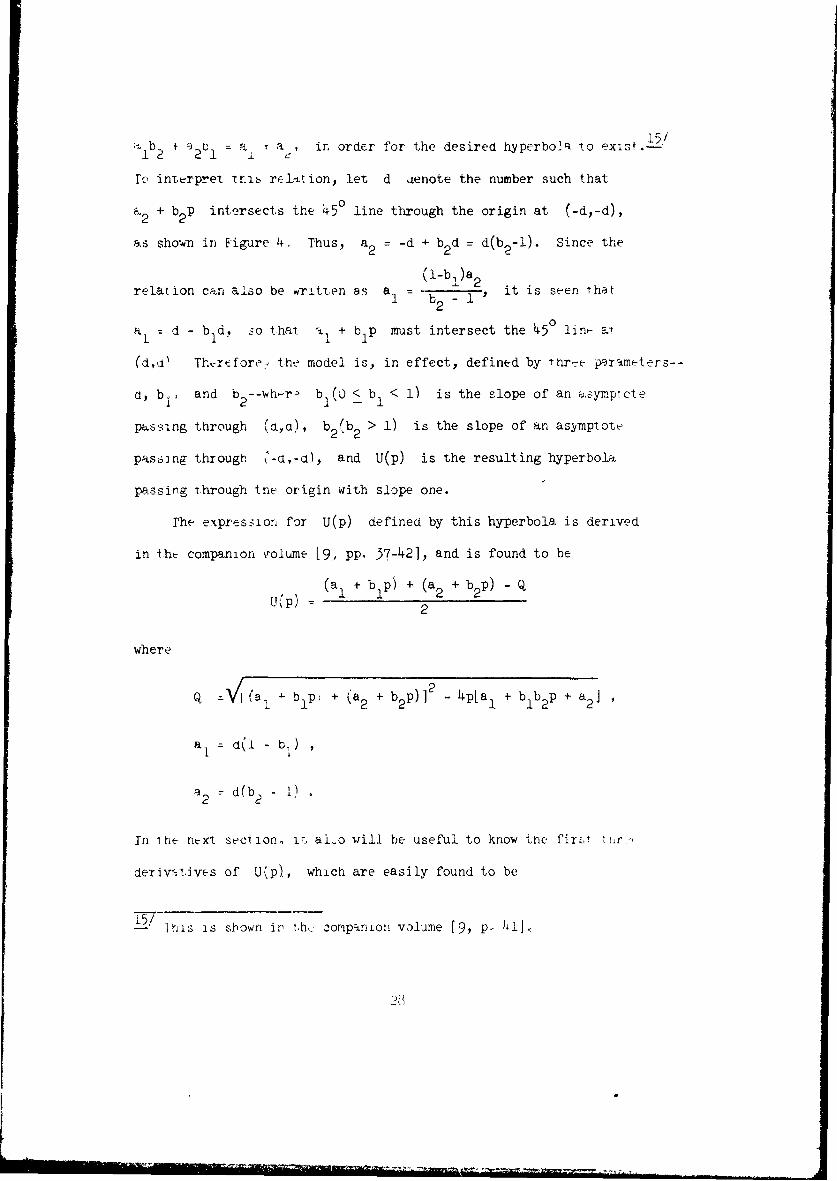
•Ib 2 ÷•2oi ) a a ¶ in order for the desired hyperbo2. io exisf.to

To intt=rprelt i•mb relttion, let d denote the number such that

2 + b2 P intersects the 450 line through the origin at (-d,-d),

as shown in Figure 4,. Thus, a 2 = -d *- b2 d = d(b_-l). Since the

(l-b,)a 2relation can also be wTitten as al = . b -i I it is seen That

2

a = d - b d, so that %1 + b p must intersect the 45° lin.- a-

(d,ql ThxEfore:, the model is, in effect, defined by T nr,.t- porameters--

d, b[, and b2 -- wh.r, b (0 < b1 < 1) is the slope of an &.sympicte

passing through (ud), b (b > 1) is the slope of an asymptote2' 2

passsng through (-i,-a), and U(p) is the resulting hyperbola

passing through the origin with slope one.

The expression for U(p) defined by this hyperbola is derived

in tht companion volume [9, PP. 57-42], and is found to be

(a1 + b p) + (a 2 + b2p) - Q

\P) = 2

where

b + p (a - p) 2 - 4p[aI + b b2 p + a2 ]

a d(i - b ,

2 d(b 2 - 1).

In ihe next seciion, ir, aLo will be useful to know thne fir•,,irf',

derivatives of U(p), which are easily found to be

157[- ihis is sbown ir t.h,: ,orapr~nion volume [9, p, 4iJ,

L.

b 1 + b 2 T

( ( T)2 - 2(b 2 - b1)2

U (P) 2Q J

u()(p) u(2)(P) T

2 ~Q2

where

T = (b 2 - b1 )2 p + (a1 + a2)(b + b2 - 2)

Thus, in order to construct U(p) for the basic model, it is

only necessary to obtain judgment decisions from management that lead

to eftimates of d, bl, and b . The question to be considered now

is how to interpret each of these three parameters of the model in a

relatively nontechnical way, so that the needed information can be

obtained from management in terms meaningful to them. To this end,

note that (-d,-d) is the point in Figure 4 at which the "piece-wise

linear approximation" of U(P), (the dashed-line function in the

figure), changes from a slope of b2 to a slope of one. Hence,

roughly speaking, the additional detrimental effect of each incremental

dollar (or larger denomination) of loss is comparable to that for the

first dollar if the total loss is somewhat less than d, whereas it

is considerably more serious if the total loss is somewhat larger than

d. Thus, when examining the effect of increasingly large losses, d

is the magnitude of loss above which the situation would deteriorate

at an accelerated rate. This interpretation of d can be explained

to management in terms of the ability to absorb additional losses.

Thus, when the total loss (in present value) is relatively small, an

29

ti(iitional dollar (or another meaningfully large denomination of money)

of' loss can be absorbed almost as easily as the first one. However,

when the total loss is already relatively large, an additional loss

would be much more serious and difficult to absorb. What is the point

of demarcation between these two situations? How large can the loss

be oefore it has become much more difficult to absorb any additional

loss? After a suitable explanation, management's answer to this kind

of question provides the desired estimate of d.

To interpret b1 and b2 , recall that the marginal utility (the

slope of U(p)) is essentially one when p is close to zero, essen-

tially b1 when p is very large, and essentially b 2 when p is

a very large negative number. Therefore, b and b2 essentially

measure the relative desirability of an incremental dollar of present

value when a very large gain or loss had already been incurred,

measured in "equivalent dollars" of worth corresponding to the desira-

bility of an incremental dollar when the realized present value had

been close to zero. To make this more concrete, it is suggested that

the following hypothetical situation be posed to management. Suppose

that a project has already been approved (to the exclusion of all other

proposed investments) that will lead to one of two possible outcomes.

The first possibility is that it will "break even," yielding a present

value of zero. The second possible outcome is that the project will

"make it big," yielding a very large gain much larger than d.

Furthermore, the two outcomes are equally likely, i.e., each has a

50-50 chance of happening. Finally, a further moderating action is

available that would have the effect of making this project less of

30

an all-or-nothing proposition. In particular, if the project woild

have broken ever, this action would add a gain of one unit of money

(a meaningfully large denomination) of present value. On the other

hand, if the project would have made it big, the action would decrease

the very large present value by x1 units of money. Should management

approve this moderating action? This obviously will depend on the

size of xI, the price that must be paid for this "insurance." The

question that needs to be answered by management is, "what is the

break-even value of xI, below which the action should be approved

and above which it should not?" Given this break-even value, call it

x*, it is then simple to verify that "ie desired estimate of b is

b 1/X1

To estimate b2 , management should consider a very similar

hypothetical situation. The one difference is that, instead of

perhaps breaking even, the first possibility for the outcome of the

project is that a very large loss (d or larger) in present value

will be incurred. Nevertheless, the firm is already committed to this

project. However, a moderating action again can be undertaken now if

desired. Thus, if the very large loss would have occurred, this

ection would decrease the loss by one unit of money. As before, if

the very large gain would have been attained, the action would decrease

the gain by some amount, which will be denoted here by x2 . The

corresponding question again needs to be answered by management,

namely, "what is the break-even value of x2, below which the moder-

ating action should be approved and above which it should not?"

Given the break-even value x., the desired estimate becomes

b 2 = x~bI = x*/x*

The second model for U(p) differs fronm the above one only in

the behavior of the utility function as p grows very large in the

negative direction. Thus, rather than assuming that U(p) converges

to a linear asymptote a2 + b 2 p as this happens, it is instead

assumed that U(p) decreases exponentially as p - - w, as shown

in Figure 5. Therefore, the algebraic form of the function is

ta-,U(p) a1 + bP - ale

where the constants for the last term are implied by -he convention

that U(O) = 0 and U(1)(O) = 1. (As before, it is assumed that

aI > 0 and 0 < b < 1.) It is then straightforward to find the

first three derivatives as

u(1) b + (1 )e

2 T-bl1U (p) (l-ba11 e•a b

u()(1 -11- -il- e )

(3)I i-b!3 au(2)(p) a a( ) eT•

Since the marginal utility (or marginal negative utility for p

decreasing) U(1 (p) increases indefinitely as p - - rather than

approaching a constant, this model exhibits an even greater aversion

32

u (p)

a+bP -

(kd, kd)

Figure The high risk aversion model for U(p).

---goo) /fwpw=x

to very large losses than the basic model. Therefore, it will be

referred to hereafter as the "high risk aversion" model.

Just as for the basic model, the high risk aversion model can

also be expressed in terms of the three parameters, d, bl, ard b2'

although their precise meaning is somewhat different here. From a

mathematical viewpoint, , now is a somewhat arbitrary large constant

(although its interpretation from management's viewpoint is similar

to before). b1 is the slope of the asymptote a1 + b1p which U(p)

converges to as p - + -, just as before) but b2 now is defined

as

b2 = U(1)(-d),

the marginal utility at a loss in present value of d. Therefore,

bel-bl-

b2 b 1 (1 - b l)e

so that

(n b d a 1 (da]

where in denot-s the logarithm to the base e. Letting k denote

k = i/ b

a, thereby becomes

a. = (1 - b )kd

w •1 1 ..

Hence, the asymptote aI + b1p must intersect the 45° line through

the origin at (kd,kd), as shown in Figure 5.

From the viewpoint of management, the interpretation of the judg-

ment decisions required in order to estimate d, bl, and b2 is

essentially the same as for the basic model. Thus, d may be inter-

preted to management just as before, especially if it is not clear at

the outset which of the two models is appropriate. if it is already

apparent that the high risk aversion model should be used, then there

is some additional flexibility in how the question may be posed. For

example, d may be interpreted simply as a "very large loss" above

which the situation would be deteriorating disastrously. Since d

is only a convenient benchmark value for this model, the important

consideration is that it represent a magnitude of loss that is mean-

ingful to management for measuring its aversion to risk (in the process

of estimating b2). The approach to estimating b, should be precisely

the same as for the basic model. The approach for b2 also should

be the same with the one exception that the unfavorable possible outcome

from the hypothetical project must now be a loss of d, rather than

any very large loss (d or larger) as before.

Since the difference between the two models is in the behavior of

u•'(p] (which can also be interpreted as the rate of increase of'

nc.gaLive utility when p is decreasing) as p - - -, the choice

bAtwcen them would be based on an analysis of this behavior. Thus,

if there exists a real disaster level where further losses cannot be

atsorbed reasonably, so that increasing the loss above this level

ii.creases the damage (negative utility) at an exponential rate, then

35

the high risk aversion model should be used. On the other hand, if

very large possible losses could be absorbed (albeit reluctantly), so

that increasing such a loss even further would increase the detrimental

effect at a nearly constant rate, then the basic model should be used.

This would presumedly be-the case if the total commitment for the

proposed investments would be quite small relative to the corporate

resources. If it is not clear which case applies, then management's

attitude can be assessed in the process of obtaining the judgment

decision leading to the estimate of b . In particular, after the

hypothetical situation has been posed in terms of the two possible

outcomes (a very large loss d or a very large gain), and the decision

on xý has been reached, then management should be asked if their

answer would change much if. the size of the loss for the first possible

outcome were increased significantly. An answer of yes would suggest

that U(,)(p) is continuing to-grow substantially as p grows very

large in the negative direction, so the high risk aversion model should

be chosen. An answer of no would suggest that u Jl(p) is approaching

a constant as p - - •, so the basic model would be the appropriate

one.

4. Finding the Best Combination of Investments

Section 2 developed a model for considering interrelationships

between investments that allows one to identify the probability dis-

tribution of present value P(6) for given feasible solutions 8.

In particular, expressions were obtained for the mean 4(b) and

2variance a (8) of this distribution, and it was indicated that the

functional form of the distribution would be at least approximately

36

normal under certain conditions. Section 3 then described how to-

construct an appropriate utility function U(p) (as a function of

the realized present value p) which formally quantifies rnanagement's

judgment on risk tradeoffs. This reduced the problem under consider-

ation to that of determining which feasible combination of investments

maximizes expected utility, i.e.,

max E(U(P(8)))

over all feasible solutions 8. What remains now is to indicate how

E(U(P(b))) can be calculated for a given 8, and then what solution

procedures can be used to find the particular feasible 8 which

maximizes this quantity.

Under most circumstances, finding the exact value of E(U(P(8)))

is not a straightforward. task, since this requires calculating the

expected value of a rather complicated function U(') of a random

variable P(8) having perhaps a very complex probability distribution.

However, one exception is when P(6) has a normal distribution and

U(p) has the form described by the high risk aversion model. For

this case, the expected utility is found in the companion volume

[9, p. 43] to be

-b 1-b (8)/2

E(U(P(8))) = a + bpl(&) - a e

where a1 and b are defined in the preceding section. In most

other cases, it is necessary to develop an approximation of E(U(P(8))).

As shown in [9, pp. 35-37], this can be done very easily by using a

37

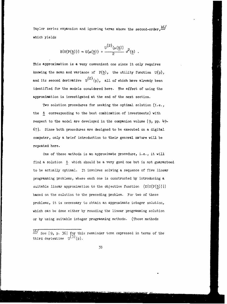
16/Taylor series expansion and ignoring terms above the second-order,-

which yields

U(2)(()

EIU(P(8))) - U(ýi(8)) + 2 a2(8)

This approximation is a very convenient one since it only requires

knowing the mean and variance of P(b), the utility function U(p),

and its second derivative U(2)(p), all of which have already been

identified for the models considered here. The effect of using the

approximation is investigated at the end of the next section.

Two solution procedures for seeking the optimal solution (i.e.,

the 8 corresponding to the best combination of investments) with

respect to the model are developed in the companion volume [9, pp. 49-

67). Since both procedures are designed to be executed on a digital

computer, only a brief introduction to their general nature will be

repeated here.

One of these methods is an approximate procedure, i.e., it will

find a solution 8 which should be a very good one but is not guaranteed

to be actually optimal. It involves solving a sequence of five linear

programming problems, where each one is constructed by introducing a

suitable linear approximation to the objective function (E(U(P(8))])

based on the solution to the preceding problem. For two of these

problems, it is necessary to obtain an approximate integer solution,

which can be done either by rounding the linear programming solution

or by using suitable integer programming methods. (These methods

±6/ See [9, P. 361 for this remainder term expressed in terms of the

third derivative P)(p).

38

include the highly efficient heuristic procedures developed elsewhere

b the author [6] or, if the problem is not too large, the algorithm

given by Petersen [15] and Geoffrion [3].

integer solutions (usually the second one) is the desired approximate

solution.

Since computer codes for solving a linear programming problem are

widely available and very efficient, the approximate procedure provides

a convenient approach that can even be used on extremely large problems.

Furthermore, as Weingartner [17] has found, linear programming is a

powerful tool for the further analysis of the problem. For example,

the dual evaluators provide vital information for studying whether it

would be worthwhile to increase the initial allocation of scarce

resources (such as budgeted funds) available for the proposed invest-

ments. Another crucial advantage is the ease with which an extensive

sensitivity analysis of the input parameters of the model may be

conducted.

The second solution procedure is an exact one, i.e., the solution

6 it obtains is definitely optimal with respect to the model and

objective function used. It is based on the branch-and-bound

teciique,17/ inasmuch as the procedure consists of applying a special

18/new branch-and-bound algorithm for integer nonlinear programming--

to first a subproblem and then to the original problem. The objective

of the subproblem is to find the feasible solution 8 which maximizes

See Hillier and Lieberman [11, pp. 565-570] for an elementarydescription of this technique.

L8/ This algorithm is presented in the companion volume [9, pp. 53-60].

39

expected present value E(P(b)). This solution is used to structure

the original problem in such a way that the branch-and-bourid algorithm

can then be applied directly to it.

Although the exact procedure is not computtLtionaly feasible for

the very large problems that can be handled by the approximate pro-

cedure, it is quite efficient Cor problems of moderate size (approxi-

mately ten investment proposals). The branch-and-bound approach is

not as well-suited as linear programming for sensitivity analysis,

etc., so it may sometimes be advantageous to apply both procedures.

Furthermore, the two integer solutions obtained in the course of the

approximate procedure can be used to expedite the respective appli-

cations cf the braxich-and-bound algorithm in the exact method.

Computational experimentation measuring the efficiency of the

two solution procedures; and the effectiveness of the approximate

procedure in obtaining good solutions, is reported in the next section.

5. Computational Experience

In order to evaluate the two solution procedures described in theig/

preceding section, ALGOL codes were developed for the IBM-36o/67.l9/

For the two phases of the approximate procedure where an approximate

integer solution is required, one of the heuristic procedures for

integer programming developed by the author [6] was used.-O/ The

19/ The author wishes to express his great appreciation to Ilan Adler

and Mrs. Patricia Peterson for developing the codes, and to FranciscoPereira for running them to obtain the computational results given inthis section.

20/ The procedure used i6 labeled 1-2A-1 in [6].

4o

main objective in d,.signing the codes was reliability rather than

efficiency or operational convenience.

The next step was to generate all of the parameters described in

Section 2 for ten basic test problems, each involving ten investment

proposals (m = 10). This was done on the computer by randomly

generating some integers from each of the intervals indicated in

Table I.- In the case of the 1jk and Pjk (k > J), some of

them were randomly selected to have a value of zero according to a

pr.;sperified probability given in the second column of Table I, and

only the rest of them were assigned randomly generated integers. In2

the case of the a., another parameter s was generated instead,2

and then used to calculate a in different ways to obtain a variety

of risk profiles, as will be described shortly. Each of the test

m

problems includes five constraints of the form, D aJk~k -< bJ

(which might, for example, represent budget constraints in the first

five time periods), arjd these ajk and b also were randomly

generated from the intervals indicated in Table I.

21/ A square bracket at the end of an interval indicates that the

end-point is included among the integers eligible for random selection,whereas a round parenthesis indicates that it is not included.

.41

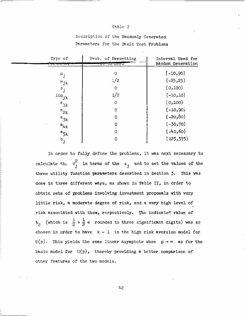
Table I

Description of the Randomly Cenerated

Parameters for the Basic Test Problems

Type of Prob. of Presetting Interval Used for

Q__4,_L:_IU Random Generation

0o [-10,90)

[Ijk 1/2 (-25,25)

s 0 [0,100)

lopjk 1/2 (-i0,i0)

alk 0 [0,100)

a 2 k 0 [-10,90)

a k 0 [-20,80)

a4k 0 [-30,70)

a5 k 0 [-4o,6o)

b 0 [125,375)

In order to fully define the problems, it was next necessary to

2calculate thc a in terms of the s and to set the values of-the

three utility function parameters described in Section 3. This was

done in three different ways, as shown in Table II, in order to

obtain sets of problems involving investment proposals with very

little risk, a moderate degree of risk, and a very high level of

risk associated with them, respectively. The indicated value of1 +1

b2 (which is 1 + 2 e rounded to three significant digits) was so

chosen in order to have k = 1 in the high risk aversion model for

U(p). This yields the same linear asymptote when p - • as for the

basic model for U(p), thereby providing a better comparison of

other features of the two models.

42

Io

I'able II

Value of the Fixed Parameters for the

Basic Test Problems

Low Risk Moderate Risk High RiskParameter Problems Problems Problems

S2 = 2 2 3a. (.= S. a . =S

3 j 3 jd 40 40 200

b 0.5 0.5 0.5

b 1.86 1.86 1.86

The resulting 30 problems were then used to test the effectiveness

of the approximate procedure by comparing its solution with that

obtained from the exact procedure, as well as with the exact solution

for maximizing p(8) if risk were ignored (which is obtained from

the first phase of the exact procedure). This was done first with

the basic model for U(p), and then with the high risk aversion model

for U(p) when the distribution of P(8) is assumed to be normal.

The results are shown in Tables III, IV, and V for the three types of

problems. For each protlem and approach, the table gives (1) "E,"

the value of E(U(P(8))) for the solution obtained, (2) "p," the

value of 4(8) for this solution, (3) "cT," the value of c(8) for

this solution, and (4) "Time," the time in seconds required to obtain

the solution on an IBM 360/67 computer. For each model, the three

columns in the tables refer respectively to (1) the feasible solution

which maximizes p(8) without considering risk, (2) the solution

obtained by the approximate procedure, and (3) the optimal solution

as obtained by the exact piocedure.

i 43

Table III

Performance of the Approximate Procedure

with Low Risk Test Problems

Bsic ' ±sic Model High Risk Aversion Model

iroblem Approx. Exact Approx. ExactUsed I max ( Proc. Proc. max P(D) Proc. Proc.

E 213.0 212.5 213.) 232.5 232.0 232.5#1 P 425.0 424.o 425.0 425.0 424.o 425.0

a 10.6 8.8 10.6 io.6 8.8 io.6Time 0.73 0.78 3.02 0.73 0.70 3.04

E 264.2 237.9 264.2 284.0 257.5 284.0

#2 9 528.0 475.0 528.0 528.0 475.0 528.0a 22.9 15.7 22.9 22.9 15.7 22.9

Time 0.59 o.64 1.20 0.59 0.61 1.47

E 142.5 87.7 142.5 162.0 107.7 162.0

#3 p 284.0 176.0 284.0 284.0 176.0 284.0a 6.6 20.5 6.6 6.6 20.5 6.6

Time 1.38 o.86 8.o1 1.38 o.85 7.74

E 152.9 252.9 152.9 172.5 172.5 172.5#4 P 505.0 305.0 305.0 305.0 305.0 305.0

a 12.9 12.9 12.9 12 9 12.9 12.9Time 1.10 o. 64 3.08 1.10 o.66 3.69

E ] 29. 5 128.9 129.5 149.5 149.0 149.5#5 259.0 258.0 259.0 259.0 258.0 259.0

c 19.8 21.9 19,8 19.8 21.9 19.8Time 093 o.67 2.70 0.93 0.75 2.67

E 117.0 112.4 117.1 136.9 132.4 137.0#6 P 234.- 225.0 234.0 234.0 225ý.o 234.0

C 17,8 21.0 16.9 17.8 21.0 16.9Time 1.63 0.75 7.65 1.63 0.77 7.64

E 55.51 53.1 53.1 71.5 71.5 71.5

• ' [06.0 lu6.o 1o6.o 106.0 1o6.o 106.07 o 12.0 12o0 12.0 12.0 12.0 12.0

Time 0,78 0.75 1.95 0.78 %.67 1.99

E 167.6 167.6 167.6 187.5 187.5 187.5

,,i 5535.0 )35 0 355.0 335.0 335.0 335.0Y 29.9 20.9 20.9 20.9 20.9 20.9

Time -L 0,85 o.68 4.30 0.85 0.66 4.17

44

E 190.8 190.8 190.8 210.5 210.5 210.5S9 381.o 381.o 381.o 381.0 381.0 381.0

16.4 16.4 16.4 16.4 16.14 16.4Time 2.83 0.71 8.10 2.83 0.74 8.03

E 128.5 121.7 128.5 148.o 141.5 148.o#1o • 256.o 243.0 256.0 256.o 243.0 256.o

a 8.7 15.9 8.7 8.7 15.9 8.7Time 0.78 0.71 4.24 O.78 0.71 4.21

E 155.9 146.6 156.0 175.5 166.2 175.5Average P 311.3 292.8 311.3 311.3 292.8 311.3

a ,, 14.9 16.6 14.8 14.9 16.6 14.8Time 1.16 0.72 3.42 1.16 0.71 4.46

45

Table IV

Performance of the Approximate Procedure

•,ith Moderate Risk Test Problems

Basic Model High Risk Aversion ModelBa sic ____

Probl. Approx. Exact Approx. ExactUsed max p(E) Proc. Proc. max V(8_) Proc. Proc.

E 207.9 208.0 208.0 232.5 232.5 232.5# P 425.0 424.0 424.o 425.0 425.0 425.0

a 80.2 75.4 75.4 80.2 80.2 80.2Time 0.73 0.73 2.71 0.73 0.76 3.61

E 242.9 228.5 242.9 282.6 257.5 282.6#2 528.o 475.0 528.o 528.o 475.0 528.o

a 183.5 115.9 183.5 183.5 115.9 183.5Time 0.59 o.65 2.46 0.59 o.61 2.19

E 139.5 111.9 139.5 162.0 -109.6 162.0

#3 1 284.0 236.0 284.0 284.0 176.0 284.0a 50.5 67.8 50.5 50.5 147.3 50.5

Time 1.38 o.78 .7.40 1.38 o.85 7.99

E 142.0 144.3 144.3 172.3 172.3 172.3#4 9 305.0 289.0 289.0 305.0 305.0 305.0

a 99.6 24.8 24.8 99.6 99.6 99.6Time 1.10 o.66 3.27 1.10 o.66 3.15

E 95.6 97.0 110.9 34.7 -724.6 134.3#5 P 259.0 216.0 229.0 259.0 258.0 229.0

a 162.2 85.7 53.1 162.2 180.9 53.1

Time 0.93 o.68 2.88 0.93 o.67 3.75

E 93.0 95.0 101.5 125.5 -522.4 133.4pI 234.0 234.0 229.0 234.0 225.0 229.0a 130.2 130.2 95.5 130.2 170.8 95.5

Time a.63 0 ,76 6.25 1.63 0.79 8.05

E 20.9 30.1 30.1 38.5 57.5 57.5#7 106.0 75.0 75.0 106.0 98.0 98.0

1 101.1 42.0 42.0 101.1 78.0 78.o

Time 0.78 0.60 1.82 0.78 o.69 2.13

E 140.7 140.7 140.7 166.2 166.2 166.2

#8 335.0 335.0 335.0 335.0a 164.3 164.3 164.3 164.3 164.3 164.3Time 0.85 o.69 4.72 o.85 0.71 5.01

,L6

FiE 178.6 178.6 178.6 210.14 210.4i 210.4

#9 381.o 381.o 381.o 381.o 381.o 381.oa 118.4 18..4 118.4 118.4 118.4 118.4

Time 2.83 0.70 7.35 2.83 0.72 8.03

E 124.6 112.9 124.6 147.9 134.8 147.9

#10 256.0 241.0 256.0 256.0 243.0 256.0Sa 54.9 76.o 54.9 54.9 126.2 54.9

Time 0.78 o.69 4.25 0.78 0.72 4.36

E 138.6 1,%.5 142.1 157.2 -12.5 169.9

Average t 277.8 290.6 221.1 277.8 292.1 307.0a 114.5 90.0 86.2 114.5 128.2 97.8

Time 1.16 0.69 4.31 1.16 0.72 4-84

47

... ..... ~~~ .....- .. . ..... ... . . .

Table V

Performance of the Approximate Procedure

with High Risk Test Problems

Basic Model High Risk Aversion ModelBasic ..

Problem Approx. Exact Approx. ExactUsed max (b) Proc. Proc. max g(E) Proc. Proc.

E -101 40.0 56.9 -1384 -1082 18o.3

#1 A 425 95 281 425 424 281a 630 53.8 268 630 617 268

Time 0.73 o.76 3.65 0.73 0.73 6.60

E -1050 -7558 0 -9.8xlO11 -734.6 64.6#2 1 528 370 0 528 314 91.

a 1431 1017 0 1431 556 139Time 0.59 0.64 4.91 0.59 o.6o 24.98

E -112 -212 77.9 -118 -343 166.6

#3 9 284 236 219 284 236 276a 465 482 149 465 482 289

Time 1.38 o.82 6.92 1.38 0.78 6.OO

E -541 -541 41.1 -55,571 -35,230 164.5#4 P 305 305 261 305 231 261

a 792 792 267 792 750 267Time 1.10 0.72 3.78 1.1o 0.71 3.43

E -2468 48.2 48.2 -6.2xo10° 100.2 100.2#5 4 259 118 118 259 118 118

a 1411 68.9 68.9 1411 68.9 68.9Time 0.93 O.60 5.74 0.93 o.61 5.96

E -1207 27.3 27.3 -3,042,622 47.9 52.6#6 1 234 51 51 234 51 81

a 959 15.6 15.6 959 15.6 152Time 1.63 o.63 4.53 1.63 o.-64 5.46

E -2261 -47.2 0 -554,102 -36.0 30.9#7 O6 43 0 106 75 43

a 856 96.2 0 856 272 96.2Time 0.78 0.59 1.61 0.78 o.66 1.-70

E -1622 48.6 48.6 -8.1xlOIO 114.9 114.9#8 P 335 142 142 335 142 142

a 1332 103 103 1332 103 103

Time o.85 o.67 2.70 o.85 O. 65 3.32

48

rrE -514 -473 51.2 -312,930 -239 16o.6

381 122 146 381 250 269a 892 442 103 892 472 289

Time 2.83 0.6 8.91 2.83 0.67 9.45

E -60.5 95.7 95.7 57.9 57.9 154.7#10o 256 188 188 256 256 188

a 381 24.o 24.o 381 381 24.0Time 0.78 0.64 3.13 0.78 0.70 3.35

E -993.6 -176.9 45.7 -1.123•XIO11 -37344.4 119.0Average p 311.3 167.0 140.6 311.3 209.7 175.0

a 914.9 309.5 99.9 914.9 371.8 159.6Time 1.16 0.60 4.26 1.16 0.68 7.51

"a 49

-I- - -! , ! . .....

An examination of these three tables reveals that the approximate

procedure obtained the optimal solution in slightly less than half of

the problems. For the low risk test problems, optimality was attained

in four of the ten cases with both models for U(p), and the objective

function was within 10% of the optimal value in five of the remaining

six problems. The optimal solution was obtained for five of the ten

moderate risk problems. For the high risk test problems, the optimal

solution for the basic model was obtained four times, and the optimal

solution for the high risk aversion model was obtained in two cases,

but the solution was far from optimal for most of the other problems

of this kind. However, the approximate procedure was successful in

surpassing the max g(_) solution (the best solution if risk were

ignored) in eight of the ten high risk test problems (with a tie in

one of the remaining two cases).

The results described are all for problems having essentially the

same set of values for the parameters of U(p). Therefore, a number

of different changes were made in these parameter values and incorpor-

2 2ated into the moderate risk version (i.e., a. = ) of test problem

5 and the high risk version (i.e., a = s 3) of test problem 6. The

objective was to gain some insight into both the effectiveness of the

approximate procedure and the behavior of the solutions as the utility

function changes. The results are shown in Tables VI and VII, where

the first three columns indicate the parameter values used for each

run. In order to provide a convenient standard of comparison, the

first set of rows repeats the results with the original set of parameter

values from the preceding tables.

50

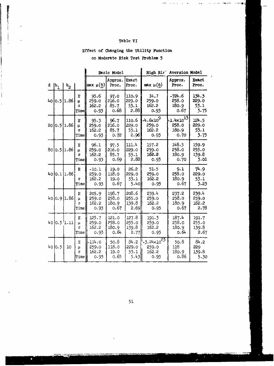
Table VI

Effect of Changing the Utility Function

on Moderate Risk Test Problem 5

Basic Model High Rir' Aversion Model

Approx. Exact Approx. Exactd b b max P(_) Proc. Proc. max Proc. Proc.

E 95.6 97.0 110.9 34.7 -724.6 134.340 0.5 1.86 p 259.0 216.0 229.0 259.0 258.0 229.0

a 162.2 85.7 53.1 162.2 180.9 53.1Time 0.93 o.68 2.88 0.93 o.67 3.75

E 95.3 96.7 110.6 -4.6x1o9 -1.4xo1 13 124.520 0.5 1.86 p 259.0 216.0 229.0 259.0 258.0 229.0

a 162.2 85.7 53.1 162.2 180.9 53.1Time 0.93 0.72 2.96 0.93 0.70 3.75

E 96.1 97.5 111.4 157.2 148.5 159.980 0.5 1.86 p 259.0 216.0 229.0 259.0 258.0 255.0

a 162.2 85.7 53.1 162.2 180.9 139.8Time 0.93 o.69 2.88 0.93 0.70 3.01

E -10.1 19.0 26.2 51.5 9.1 74.940 o.1 1.86 259.0 118.0 229.0 259.0 258.0 229.0

a 162.2 19.0 53.1 162.2 180.9 53.1Time 0.93 o.67 5.40 0.93 o.67 3.23

E 205.9 198.7 208.6 239.4 237.2 239.44o 0o.9 1.86 p 259.0 258.0 255.0 259.0 258.0 259.0

0 162.2 180.9 139.8 162.2 180.9 162.2Time 0.93 o.67 2.69 0.93 o.67 2.78

E 125.7 -121.0 127,8 191.3 187.4 191.740 0.5 1.11 p 259.0 258.0 255.0 259.0 258.0 255.0

a 162.2 180.9 139.8 162.2 180.9 139.8Time 0.93 o.64 2.77 0.93 o.64 2.67

E -114.o 50.8 84.2 ,-3.24x1o23 50.8 84.24o 0.5 10 P 259.0 118.0 229.0 259.0 118 229

a 162.2 19.0 53.1 162.2 180.9 139.8Time 0.93 o.65 5.43 0.93 o.86 5.30

51

Table VII

Effect of Changing the Utility Function

on High Risk Test Problem 6

Basic Model High Risk Aversion Model

Approx. fact Approx. Exactd bI b2 1 m ;(8A) Proc. P.oc. max P(8) Proc. Proc.

E -1207 27.3 27.3 3,042,622 47.9 52.6200 0.5 1.86 A 234 51 51 234 51 81

a 959 15.6 15.6 959 15.6 152T1me 1.63 O.63 14.53 1.63 o.64 5.46

E -1213 26.0 26.0 -4.4xO 2°0 45.3 45.3100 0.5 1.86 P 234 51 51 234 51 51

a 959 11.2 11.2 959 11.2 11.2Time 1.63 0.66 4.54 1.63 o.67 5.87

E -1197 -880 29.6 -1655 65.5 84.34o0 0.5 1.86 p 234 105 51 234 81 151

a 959 545 11.2 959 149 326Time 1.63 0.65 4.55 1.63 o.66 5.04

E -1709 30.6 30.6 -21,108 47.1 47.1200 0.1 1.86 V 234 51 51 234 51 51

a 959 11.2 11.2 959 11.2 11.2Time 1.63 o.65 4.43 1.63 o.66 5.04

E -103 -1584 10.4 -2.0Xi'> 5.-1X)107 --200 0.9 1.86 p 234 105 51 234 225 --

a 959 545 11.2 959 533 --Time 1.63 0.66 4.89 1.63 0.67 > 180

E -841 48.3 48.3 -1o.6 74.3 122.0200 0.5 1.11 4 234 51 51 234 81 151

a 959 11.2 11.2 959 149 326Time 1.63 0.72 4.79 1.63 o.66 4.30

E -9531 13.7 13.7 -2.Ci<103 -38.3 43.2200 0.5 10 4 234 51 51 234 81 51

a 959 11.2 11.2 959 149 11.2Time 1.63 o.64 4.41 1.63 o.65 785

52

The next objective was to test the efficiency of the exact pro-

cedure with problems of different sizes. It was seen in the preceding

tables that it is quite efficient with problems having five constraints

and ten variables, requiring between one and ten seconds in all but

one of the 84 cases.22/ However, the nature of this branch-and-bound

procedure is that. its running time should tend to grow quite rapidly

with the size of the y roblem (especially as m, the number of variables

increases). In order to estimate this rate of growth, and the resulting

maximum number of variables (investment proposals) for which the pro-

cedure should be computationally feasible, some of the basic test

problems were modified and/or combined to construct problems of other

sizes. In each case, the values of the parameters shown in Table II

mwere retained with the one exception that d was multiplied by 10

All of the original values of the pji0 Pjk' sj, and Pjk also were

retained. When new values of pjk and pjk had to be introduced

because of combining problems, these new values were automatically

set equal to zero. All variables kept their same ajk coefficients

in the constraints. In those cases were the number of constraints

was reduced from five to one, this was done by eliminating all but the

constraint involving the a3k and b3 parameters. When a basic test

problem was used to contribute only half of its variables to the new

problem, the first five variables were chosen, and the values of the

b. were divided by two. When combining two basic test problems oT

22/When the high risk aversion model was used with the b = 0.9

problem in Table VII, the procedure did not terminate in three minutesof computer time. The reason is not evident.

53

portions thereof - their current values of bi were added to obtain

the bi for the new problem.

Table VIII shows the results of the runs on an IM-36o/67 system

with these new test problems. The first column indicates which basic

test problem(s) was used to construct the problem for that run, and

the next two columns give the resulting number of constraints and

variables. Th! remaining three pairs of columns identify the version

of the problem (corresponding to the three versions in Table II) and

the type of utility function model (basic model or high risk aversion

model) that were usad. To provide a frame of reference, the average

time for all of the basic test problems, as well as the individual

times for the ones used to construct new problems here, are repeated

from Tables III, IV, and V.

Recall from the preceding section that an exact expression for

E(U(P(8))) is now known only when the high risk aversion model is

being used and the distribution of P(5) is normal. Otherwise, only

an approximate expression, obtained from using a Taylor series expansion,

is available. The exact procedure finds the feasible solution that

maximizes whatever objective function is being used. Therefore, when

the approximate expression is taken to be the objective function, there

is no guarantee that the resulting solution will be the exact optimal

solution for the real problem. Thus, it is important to verify that

this approximation really is an adequate one, especially in terms of

the resulting solution still being at least nearly optimal.

It is straightforward to study this question analytically for

the case of the high risk aversion model. Define

54

N c~ LIt- 0IC% 0 rOH ~CUP:; c ei% (M 14. Ov i %O "'N \0 0

66 o0'.' U\ % U NKA

\D p.0 a\ O0 t1r-t -10 0 0ai cu K'1 -t 0 -t \D * t-- t-

ca -1 0 0 W O

o~G Aou.

o 0) H w 46HO c LAuý .

1-4 w.

ws s u nn

(D )4 0 r4 C)\ .C .47- t'\ I.c0 -.-~ ~-t 0 0 0 HOJcu 0Jc'J Ct

H 4-1 r ~ A

w 0

as *rlw El-.E-1 94H -.4

Q .,f.

E-11

;4 to*0

0 0o

www

0.0CH 0

E-i10ý-i H -ol~ HH HH H Hl~ HOI C\JCl~

z055

c = 1 "2 "

Then set p = 1(6) and substitute the expressions for U(p) and

U(2) (p) given for this model into the approximate expression for

E(U(P(5))). This yields

1l -b 1 g o

E(U(P(_)))] - aI + blp(6) - a1e( 1) [ l+c]

Now notice that the exact expression can be written as

E(U(P(6))) = aI + blp(_) - ale [l1a() c]

and that the standard expansion for ec is

c c2 c3e =i+ c + r., + 3. + . .

Thus, the approximate expression is equivalent here to expanding the

e part of the exact expression and then ignoring terms above the

first-order. The effect is to give somewhat less weight to the penalty

for risk (as measured by a(_)) than is warranted. The approximation

is quite good if c is somewhat less than one, but is quite poor if

c is somewhat larger than one. Thus, the critical factor is thea1 aI

relative size of a- and the a(_). Recall that, = kd, and1b11-b1 1

that (kd,kd) is the point at which the asymptote (a1 + b1P) of the

utility function intersects the 45 line through the origin. Thus,a1

- can be interpreted loosely as a point of diminishing returns for1-b 1

56

gains in present value. If this point is at least comparable in size

to a(5) for the interesting values of _5, then the approximation

should be quite adequate.

For the basic test problems and high risk aversion model, the value

of kd is 40 for the low risk and moderate risk versions and 200 for

the high risk version of these problems. The corresponding values of

the a(8) for interesting 5 are such that the value of c would be

a rather small fraction of one for the low risk problems, but would

tend to be approximately one or even considerably larger for most of

the other problems. Therefore, if the approximate expression for

E(U(P(_))) were to be used instead of the exact one, it appears that

the exact procedure should still give very good solutions for the

low risk problems but might not perform well for the other problems.

To test this experimentally, all 30 problems were rerun with the exact

procedure using the approximate expression. The results are shown in

Table IX. The first column identifies the problem, where LR is an

abbreviation for Low Risk, MR for Moderate Risk, and HR for High

Risk. The second column indicates the time in seconds required by the

exact procedure run inthis way, and the next two columns give the

values of iL(8) and a(8) for the resulting solution which maximizes

the approximate objective function. The fifth column recalculates

the value of the objective function for this solution by using the

exact expression. The last column then gives the ratio (expressed

as a percentage) of this value to the corresponding value for the

real optimal solution as given in Tables II, III, or IV. An examination

of this column also reveals that the solution obtained actually was

57

Table IX

Effect of Using the Approximate Expression for E(U(P(6)))

with the Exact Procedure and High Risk Aversion Model

E*Problem Time a E E

LR, #1 3.02 425 10.6 232.5 100%

LR, #2 1.47 528 22.9 284.0 100%

LR, #3 7.97 284 6.6 162.0 100%

LR, #4 3o70 305 12.9 172.5 10%LR, #5 2.66 259 19.8 149.5 100%

LR, #6 7.63 234 16.9 137.0 100%

LR,, #7 1.914 106 12.0 71.5 100%LRI, #8 L-05 335 20.9 187.5 100%

LR, #9 8.M2 381 16.4 210.5 100%LR, #10 4.21 256 8.7 148.0 loo%

LRI, Ave. 4.47 311.3 14.8 175.5 i00%

MR, #2 3.61 425 80.2 232.5 i0o%

MR, 2.16 528 183.5 282.6 100%

NR, #3 8.00 284 50.5 162.o0 OO%

MR, #4 3.08 305 99.6 172.5 1O0%

MR, #5 2.69 259 162.2 34.7 25.8%

MR, #6 7.70 234 130.2 125.5 94.2%

MR, #7 1.95 io6 101.1 38.5 67.1%

MR, #8 4.06 335 164.3 166.2 1O0%

MR, #9 8.04 381 118.4 210.4 100%

MR, #10 4.25 256 54.9 147.9 10%

MR, Ave. 4.55 311.3 114.5 157.3 88.7%

HR, #1 2.34 396 459 106.2 58.9%

HR, # 1.64 367 151 282.6 100%

HR, #3 5.11 276 289 166.6 i00

HR, #4 3.21 261 267 164.5 100%HR, #5 5.95 118 68.9 100.2 100%

HR, #6 5.31 151 326 -1.9 -3.7%HR, #7 1.69 43 96.2 30.9 i00%HR, #8 3.14 142 103 114.9 100%HR, #9 7.59. 323 420 81.3 50.6%HR, #10 3.30 188 24.0 154.7 100%

HR, Ave. 3.93 226.5 220.4 120.0 80.6%

58

r

optimal for all ten low risk problems, and for seven out of ten of

both the moderate risk and high risk problems. Staudyig the effect

of using the approximate expression with the basic model for U(p)

is more difficult. However, an analysis of the remainder term that

has been deleted from this expression suggests that it probably would

tend to be positive, and should tend to increase as a(b) increases,

so that the expression underestimates E(U(P(5))] most for large values

of a(5). Therefore, it appears that, in contrast to the conclusion

drawn for the high risk aversion model, the effect of the approximation

with the basic model is to give somewhat more weight to the penalty

for risk than is warranted. This conjecture is strongly supported by

the computational results given in this section. In those cases where

the basic model (using the approximate expression) and the corresponding

high risk aversion model (using an exact expression) obtained different

solutions on a given problem, it was always the basic model that yielded

the solution with the smaller value of a(E), despite the less con-

servative utility function for this model.

6. Conclusions

The companion volume [9] comprehensively studies the problem of

evaluating risky interrelated investments. One basic approach developed

there has been selected for further study and elaboration here. This

approach involves considering the probability dist. .bution of present

value for alternative combinations of investments, and then using

powerful solution procedures to seek the feasible combination that

maximizes the expected value of a utility function of present value.

It takes into account various kinds of interrelationships between

59

the proposed investments in some relatively convenient ways.

The utility function approach to considering risk is a relatively

sophisticated technique that usually has been shunned in practice in

favor of subjective evaluation of risk profiles by management. However,

when a substantial number of proposed projects are being evaluated

simultaneously (due to such interrelationships as competing for the

same capital resources), so that the number of possible investment

combinations is huge, it is then necessary to use some other device

to identify the few best alternatives for careful evaluation by manage-

ment. The utility function approach is a powerful and flexible way of

doing this. Furthermore, a practical way of constructing a reasonable

utility function by merely obtaining three meaningful judgment decisions

from management has been developed in Section 3. Computational experience

(see Tables VI and VII) also suggests that the optiual solut 4 on tends

to be not too sensitive to the choice for each of these decisions.

Therefore, the use of a utility function in this way appears to be

a much more attractive and practical approach to the problem than

might have been anticipated.

A useful area for future research would be a behavioral study of

the process by which management would make the three judgment decisions

described in Section 3 and of how the resulting answers would relate

to management's true preferences on risk tradeoffs. This might lead

to a refined procedure for obtaining the required information from

management.

It is important to recognize that, when trying to identify the

best combination of investments, it is the risk profile for the

60

II

combination (primarily p(_) and 0(_))) that is crucial rather than

the risk profiles for the individual investments. Thus, even though

a number of proposals appear individually to be very risky (i.e., 0

jjSis large relative to I•j), there may still be an acceptably small

degree of risk associated with approving all of these investments

jointly. This diversification effect occurs because 0(_) tends to

grow less rapidly than V(5) as more investments are approvedp'

and this effect is even more pronounced if some of the P are nega-

tively correlated. Thus, it is dangerous to rely too much on sub-

jective or compartmentalized decision-making here.

Computational experience suggests that the approximate solution

is fairly effective in obtaining good solutions (and slightly more so

when using the basic model for U(p) rather than the high risk aversion

model), since it actually yielded the optimal solution for almost

half of the test problems. However, it does tend to give somewhat

lens weight to the element of risk than is warranted. As a result,

it may yield a poor solution when considering a very risky set of

proposed investments. Therefore, it is especially important in this

situation to calculate the value of E(U(P(5))) for the solution 8

obtained in order to verify that this value actually is positive and

reasonanly large. It also would be advisable to rerun the procedure

2several times with more conservative values of the C2 and of the

parameters of the utility function to see if less risky solutions

yielding a higher expected utility are obtained.

2-/ For example, if N independent and identically distributed invest-ments are approved, then a(8) = fliaN whereas p(8) = J.

61

Since the approximate procedure is based primarily on using linear

progamming, it can handle a large number of constraints with ease,

and is cor autationaily feasible for problems involving an extremely

large number of investment proposals. It also is quite well-suited

for conducting an extensive sensitivity analysis (by referring to the

final fractional solution rather than the final integer solution).

Another advantage is +hat it can be readily adapted to the case where

some of the investment decisions are of the "how much" rather than

"yes-or-no" type.

The exact solution procedure does not enjoy any of these advantages

of the approximate procedure. However, it does, of course, have the

crucial advantage of guaranteeing an optimal solution (with respect

to the objective function used) for any problem small enough for it

to solve. It is quite efficient for problems involving approximately

ten investment proposals or less. However, the computation time grows

rapidly with the size of the problem, so it is almost certain to be

computationally feasible only up to approximately fifteen proposals.

It can also be tried with at least a small hope of success when there

are say 20 to 25 proposals. It would seem that the presence of

mutually exclusive sets of investment proposals also should increase

the efficiency, although this has not been tested.

When it is assumed that P(5) has a normal distribution and that

U(P) follows the high risk aversion model, then the corresponding

exact expression for E(U(P(5) ) should be used with the exact pro-

cedure. For other ,,ases, an approximate expression based on a Taylor

series expansion of E(U(P(ý))] is available. As discussed at the

62

end of the preceding section, this approxinate expression performs

quite well (still leading to the optimal solution in 24 of the 30

test problems run with the nigh risk aversion model), but it is

sufficiently imprecise that its effect should not be ignored. With

the high risk aversion model, it usually gives somewhat less consider-

ation to risk than it should. Therefore, even when the distribution

of P(5) is far from normal, the expression that is exact for the

normal distribution usually should be used instead in order to better

approximate the appropriate risk tradeoffs. The only exceptions might

be distributions that are skewed substantially to the rigat, since

then the risk for a given g(_) and a(_) tends to be somewhat less

than with the normal distribution. When the basic model for U(p) is

being used, the approximate expression has the opposite effect, giving

somewhat more weight to risk than is warranted. Sinre no exact

expression is-now available for the model, it is then especially

important to conduct sensitivity analysis to check for alternative

solutions that may give a better balance between risk and the expected

return in present value.

The choice between the two alternative models for U(p) should

be based both on their inherent properties (as discussed in Section 3)

and the behavior of the available solution procedures with them. It

appears that the two models should be quite comparable in their evalu-

ation of combinations of investments having only a moderate degree of

risk, but the high risk aversion model should be much less tolerant

of very risky combinations than the basic model. In effect, the hiph

risk aversion model has a threshold level of tolerable risk beyond

63

which it increases the penalty for risk very rapidly (due to the

exponential form of the function). Thus, the optimal solutions for

the two models (with respect to exact expressions for E[U(P(j))J)

should tend to be fairly comparable (and often identical), but somewhat

riskier solutions may be still rated good by the basic model but very

poor by the high risk aversion model. Because of the conservative

effect of using the approximate expression for E[U(P(!_))) with the

basic model, the solution procedures tend to occasionally yield somewhat

less risky solutions for this model than the high risk aversion model.

This effect should be .taken into account in choosing between the two

models. However, it should also be noted that this tendency may be

less pronounced (and perhaps even reversed) when the utility function

parameters are such that k is somewhat less than one (which wouli

be common) in the high risk Lversion model rather than the value of

one used for almost all of the computational experimentation. A final

factor in making the choice is that the approximute solution procedure

appears to be at least slightly more effective in obtaining good

solutions with the basic model than with the high risk aversion model.

In conclsion, it should be reemphasized that the main prrctical

purpose of this approach to analyzing risky interrelated investments

is to identify and quantitatively describe the few best combinations

of investments for careful evaluation by management. Thus, rather

than using one set of parameter values, one utility function, and

one solution procedure to find "the optimal solution," it usually is

important to conduct r sensitivity analysis on the data to identify

those solutions that are best under some plausible set of estimates.

64

This may well involve using more than one utility function model and

t solution procedure, much like in Tables VI and VII. This process

will identify a small number of alternatives requiring further con-

sideration, and will provide relevant quantitative measures of

performance (g(5),_ '(5), the'resulting risk profile, and E(U(P(l))))

for these alternatives under different assumptions. Management can

then analyze this information, as well as other relevant factors not

incorporated into the model, and make its decision on the best combi-

nation of investment proposals to approve.

65

CITED REFERENCES

(See [9, pp. 101-110] for a comprehensive bibliography)

1. Byrne, R. F., Charnes, A., Cooper, W. W., and Kortanek, K. 0.,

"A Chance-Constrained Programming Approach to Capital

Budgeting with Portfolio Type Payback and Liquidity Con-

straints and Horizon Posture Controls," a chapter in [18].

2. Byrne, R. F., Charnes, A., Cooper, W. W., and Kortanek, K. 0.,

"A Discrete Probability Chance-Constrained Capital Budgeting

Model," a chapter in [18].

3. Geoffrion, Arthur, "An Improved Implicit Enumeration Approach for

Integer Programming," Operations Research, Vol. 17 (1969),

pp. 437-454.

4. Hertz, D. B., "Risk Analysis in Capital Investment," Harvard

Business Review, Jan.-Feb., 1964., pp. 95-106.

5. Hillier, 7rederick S., "Chance-Constrained Programming with 0-1

or Bounded Continuous Decision Variables," Mana ement Science,

Vol. 14, No. 1 (Sept., 1967), pp. 34-57.

6. Hillier, Frederick S., "Efficient Heuristic Procedures for Integer

Linear Programming with an Interior," Operations Research,

Vol. 17, No. 4 (July-Aug., 1969).

7. Hillier, Frederick S., "Supplement to 'The Derivation of Proba-

bilistic Information for the Evaluation of Risky Invest-

ments'," Management Science, Vol. 11, No. 3 (Jan., 1965),

pp. 485-487.

66

II

8. Hillier, Frederick S., "The Derivation of Probabilistic Infor-

mation for the Evaluation of Risky Investments," Management

Science, Vol. 9, No. 3 (April, 1963), PP. 443-4571 alsoreprinted in (i) J. Van Horne (ed.), Foundations for

Financial Management: A Book of Readings, Irwin, Homewood,

Illinois, 1966, pp. 310-326j (ii) S. H. Archer and C. A.

D'Ambrosio (eds.), The Theory of Business Finance: A Book

of Readings, MacMillan, 1967, pp. 422-437; (iii) E. J.

Mock (ed.), Financial Decision Making, International Textbook

Company, Scranton, Pa., 1967, pp. 422-4361 (iv) H. Albach

(ed.), "Reader on the Theory of the Firm II: Long-Range

Planning and the Theory of Investment of the Firm,"

Kiepenhener and Witsch Verlag, Cologne, forthcoming (in

German); (v) R. Bruce Hicks (ed.), Portfolio Management,

McGraw-Hill, New York, forthcoming.

9. Hillier, Frederick S., The Evaluation of Risky Interrelated

Investments (Vol. 1 of the TIMS-ONR monographs on "Budgeting

Interrelated Activities"), North-Holland, Amsterdam, 1969.

10. Hillier, Frederick S., and Heebink, David V., "Evaluating Risky

Capital Investments," California Management Review, Winter,

1965-66, pp. 71-8o.

11. Hillier, Frederick S., and Lieberman, Gerald J., Introduction to

Operations ReseRrch, Holden-Day, San Francisco, 1967.

12. MErkowitz, Harry M., Portfolio Selection, Wiley, New York, 1959.

13. Naslund, Bertil, "A Model of Capital Budgeting Under Risk," a

chapter in [18].

67

)4. Naslund, Bertil, Decisions under Risk, The Economic Research

Institute, Stockholm School of Economics, 1967.

15. Petersen, Clifford C., "Computational Experience with Variants

of the Balas Algorithm Applied to the Selection of R & D

Projects," Management Science, Vol. 13, No. 9 (May, 1967),

pp. 736-750.

16. Weingartner, H. Martin, "Capital Budgeting of interrelated

Projects: Survey and Synthesis," Management Science,

Vol. 12, No. 7 (March, 1966), pp. 485-516.

17. Weingartner, H. Martin, Mathematical Programming, and the

Analysis of Capital Budgeting Problems, Prentice-Hall,

Englewood Cliffs, N. J., 1963.

18. Byrne, Robert F. (ed.), New Approaches to Budgeting (Vol. 2 of

the TIMS-ONR monographs on "Budgeting Interrelated Activities"),

North-Holland, Amsterdam, forthcoming. This collection of

invited papers will include the text but not the appendix

of this report.

68

APPENDIX

Listing of Test Problems

This appendix presents the ten basic test problems that were

randomly generated as described by Table I of Section 4. The numbering

of the problems coincides with that used in the various tables. For

each problem, the diagonal elements of "MU-MATRIX" are the gji in

order, and the off-diagonal elements are the p jk The diagonal

elements of the second matrix in each listing are the sj, and the

off-diagonal elements are the pjk" The third matrix lists the a.k

and, on the far right, the b..

69

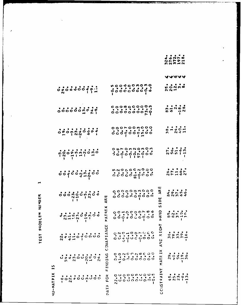
OY re

O.o000 0

M4' 0' co *0 N 0* wOe

N~~~ tAOOC O LA"

0* 0

0~ ~ ~ n 0 n 0 0t 00 00 V0

NN IN 0000Nt

co I

00 1. *. ** *6 * 0 # * * * ,N -

IiN u4II <~~O O~ O

cO ONeO e e g ..

4z 0 OC0-400 0 0 N - O

w6 N-i IN W OOOO 00

x '

00 00006 *O e*oO 0 09~ 0 x

-J N.-e-'LL fi u~ 0 0 0 0Qo 0

C;( 1-

in 00 ,0000~ofO *t In0

0ON O O O * * * * .4, ; V* *: *

.6 *ee o (n V4 00 0000000 - %.

-~ 00000 00100

* 0 0 0 @. . . . <, A .0.00 4

w44 I 0000000000Cnr)I I u

*o m oto- I- z ** 00 0 *l 0 0 0 u 0 Q0NN <~' ..4 V40CC0u*' 0t

OtO0-00C u*.* x. ~UO'- 000 00000

C; I0 CIc 94C4W

w~oo" U-04 0~ w 0o0 006- 0ii 00 o o -I V4 -4

4 0

LcI 001'(l0f0- N- L .Lo.. cq 10 in0 0V

I~O ~ 4I < 0 04.000 0 4 '-i71

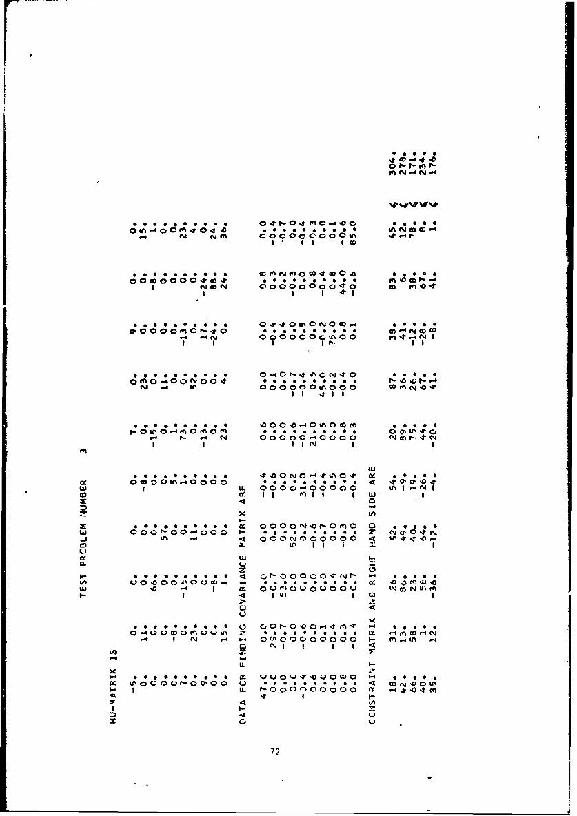
04 104 e o0%0000

goo0* 00 00 0*000; NCDC

OiA400 8.tO4t a0 0 0 0 0 a 0 000 ml~-

N00 0 0 Go 0y 00 0 00 ,9CD Po *t

4;,;00 o 00 t 0 0 0 * 0 0 0 0 0 O

N00r~0-00 0 a0 0 C0 UN0 0 0 n-

-"N OZ8888O;88 go e N.tNI I %t- I I

0.-40r-4Ir 0Nm40 00.

0~~O.40QN00t 00 In %r ***N- N cc) OoO 0tu 04

* S 0 0 00 0 0 0 0 ' A0~'40"~~ 0 * * *ac 0 0 * * 0 * * 0 * -

w- p-.- 00000400000 IA 1 P4

Wi P! W4 00 0P 00 0 00 00

40

V) %00 .01oC 0 00 ONo -o; 0 L .,o (1

UU>

0u

C;~~~ ~ 0 e OZ C0001* 0 0 0 * 9 0 f E x

-4ý ao o o m -4-

C O'j 4'~)W * 0 0

o" w. t00OU.0O 00 W .

at'3 IA I-8t; 8 :8 :

4~U,

72

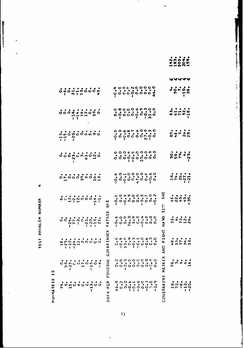
W4 D 00

B~~~ 9B. 1t OD0OO 0 0f P-Gf

00 00co0M 00

60 00 00 0z CO 4IfO OU; 8 ,0 M000 Ic&

C;,;~ tI4 N 0 * 0' 0 0 *0 4 ccC 0 OO Q4f

gB N rn f--

0 I; Iz C, m 0,

0 6 0 0 0 0 6 C;,; C;O OM OD O N r'ý 0 t0 0

.4 C4 t,

-Z C4 J ;LA8lo

*o omo o 0 0 0 %0 COC"1 0000

w- O -N r O-4 B- C;o o* * w .f-II

-J N-B N.4N .4 OO~Or~OO OO . ~ I.73

I~c InN In00~ O

'00

InO,OO O 0 c0 0 0 0 in 0CID

*~ o*0 CY0000 %000

P4 4 4 0 00 0 0

* 09000000 00~0OO00OO- .000

'M A0O 0M0 0 q 0 * 0 0 * * * -wNo-r N 1. I L OOOOMOOM00 ONw Ix41

to oo* * t~O00CJ 00

ww

4y 0

-4'4I -4 ~-C t;10 N M

U--

< 10 z

o 4m

INN 0-4'~0 ' .- CJ

zU. -

x

4- c III

74

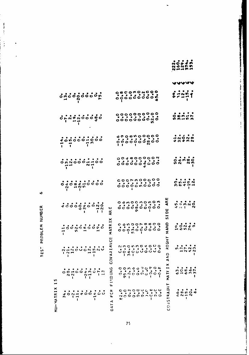
in V4

0000000000

* sO.00 0 ~o wuo 000

I e4 *

*o*04MOCOOO0

~O~fl O0'00 0 *0 r- In * 0 *. * 0N N

-e C; No 0 0 0000000000

ui~ e: 0N t (7

0050 0000 000t% 00000 Ng .

Ij I U* P- VIr

4' O 0 t 0 0 0 oo C)0()0% Pfw C-1 z L 0000 0000 6t' s N n0wQf

(m NI N,4 1CýL 0' 0 C, n 0O

4 C04C i 6 o( n0'I--

LIn

75

Ir

c; ~ ~ p c:cy, t- 0"

.NN

.. ,~~0 N NOOOCLC OP OI

C O I

N ~.* 0 0 ~~00N 9 0

0 0 a 0 * * m9

0000000000

*~~~ * ,aa 0 0 0 0

~~~*0 0 04, 9 0 -4 00ui

904.- 990 NO O OO~ *69 8000400 0 L

e-'- or ~ o c.o OD 3s-)

'ITU4

0

>-

g 099 0 0~- 0 0 0o9 * 0 V 'D 0 6 S

0..4

X ~ 0 0 9 0 0 0j 0~ 0 * 0 . ug.4'

In o . -, 0

.qIL

76

AJ 000000000 f

0~ ~ 0 a 0 1- 0 * 0~g~

I- N ~..,..000o00 0' IV N

~~~I~~ N -'0Oc O O N

Mtn* 9 0 00

4D 0008 z4Z8 .60 in M 9%'O Oor-IAOOOONOO1 0 S* 0 1 NDO

* 0.000 0, OO.~cOU~O0O*o 00.

00t; 0 - O No M 0% m 0 S0Oj CY0000OW000OO

NNI I I00000400000

0

.- NL40 00' * * ** Nw -N4s N UJ 0004000000 < (nP-t

4

z 'C

Leo Qn00 04Q. u

0%0

00. ; cou000 Col00 Of. 0 * * 0 a 0 r-

I4 1- (1 0' U.4

Q

77C

ýý N WN Uf

OQOC~~~c mO~O 09 9 ***

0 0g *90 ~oosoOr. ~ .m0 0

0.0c 000-oOO 0 0 * 0 a * 0 0a

PN .-4 OD' OOOOOOO0O N ?-o

I I iI

~~e~eO~~e~9t afooo ODO~goo05

~~ B~c N OO O O0 O c'No -lN

'4O O-'OOO 0000 9905 ONI8 00 0OCIOI-Om-TO

LU .44 I N .- 4 WL O;OOO AU1 c 8 0O OOoO O N m

LL) 0 4 '

W LL~C~OCOOU' . ~ CC~9 0*0

a.A.

50900-a 0 0c 0 CO ~ ~ u( 0 0 ,(Y4/) _0 0, *o e r. CIO * 0 . ~

0 It1

mw ~ rO 0 Q-'~ .'l 1 0 0 # 0 0 * 0 J u*IxL 1 o c".- co 0.-CO O@00 a- 0 .-j N

ý4,4I C4 U- C)0C ,jU I

b.478

t'- OD V- o&

V/ V/ V/ V/

0r~i~'O~OOOCCD 01 00 0 &*

cz 0*

**..*S0-0 Oý-0'u40 00

c;0 Z 0 0 0 a 0 0 0 0 LA 0% 0 UN-4' 41-4 000I-000

* ~~~~~0 0.0 0 C,~0.40L~4 000mg-'c c; 0C, C0 <

LU ~ ~ ~ ~ N uuj14 q0

0e 0, 00 0* 00~C, M m00C 0 q 0 000 0 0 0 0 0 * 0 '4*0*-4 X

CCJA

LU a

a- Ls0 ~ s C, 0 trl -q 1-3~ 0 0 0V) 1- 0 *0c1 0 * * * * LL 0IC.)- Q N

Ui p.. L) vr (_) ki0)L m (\ C

C. tr 4-4L

0- *oc t-- 0 o t) 0 0 0 *

'I. U- %rC r I-e t - l

CD

79

UnclassifiedSecurity

Classification

(*3.ltv ¢lesellicalI., of title. bmW .1 abstre.e and kweErltp mtaftfu see"e bde omi nd " Mo evmlI ml nI so abse•.

t. ORIGINATIN G ACTIVITY (Co..rlo sulw Se. REPORT SIECURITY C LAWlIFCA

Stanford UniversityDept. of Operations Research 2& mOti.P

Stanford, Calif. 94305S. REPORT TITLE

A BASIC APPROACH TO THE EVALUATION OF RISKY INTERRELATED INVESTMENTS

4. DKSCRIPTIVE NOTES (2TM*. of poat wiEi Inclueai do#*&)-

Technical ReportS. AUTHOR(S) (Lost name. flint nomo. Initial)

HILLIER, FREDERICK S.

6. REPORT DATE 7A. TOTAL. NO. OF PAG[ 7Tb. NO. OF ItP$

August 15, 1969 79 18

GA. CONTRACT OR GRANT NO. 9a. ORIOHNATORS8 REPONT NUMERA(S)

N00014-67-A-0112-0011 Technical Report No. 69-9b, PROJUCT NO.

NR-047-064-0. Ob. OYNEHRR JPORT NO(S) (Any cobe, munmostsssy afnjbotaasie.d

#125- Nonr-225(53) NR-042-002_ _ _ _#4 - NSF GP-7074

10. AVA IL ABILITY/LIMITATION NOTICES #12 - Nonr-225(89) NR-047-061

This document has been approved for public release and sale; its distributionis unlimited

11. SUPPLEMENTARY NOTES I2. SPONSORING MILITARY ACTIVITY

Operations Research Program (code 434)Office of Naval ResearchWashington, D. C.

13 ABSTRACT

When evaluating proposals for capital investment, it often is necessaryto consider interrelationships of various kinds between the proposed projects.The amount of risk associated with the investments also is a very importantfactor. 'This paper studies the problem of how to simultaneously take bothconsiderations into account in order to determine the best overall combinationof projects to approach. In particular, it focuses on one basic approachdeveloped in the author's monograph, The Evaluation of Risky InterrelatedInvestments (North-Holland, 1969), and extends it further in terms of formulationand interpretation needed for implementation. This approach uses present value(treated as a random variable) and expected utility of present value ascriteria.

The paper begins by discussing the nature of various possible projectinterrelationships and how to take their effects into account in the analysis.It then develops a model for also considering risk, including an easily imple-mented method of constructing an appropriate utility function. An approximatelinear programming approach and an exact integer nonlinear programming algorithmfor finding the best combination of investments are reviewed. Finally, theresults of extensive computational experimentation with these solution proce-dures are reported and evaluated.

SFORMD D 1473 UnclassifiedSecurity Classification

Ii

UNCLASSIFIED- ccurity Classification

"LiNKA UNK USK CKEY WORDS ROLEt Wy RoLl I Y WT ML[ WT

1. Budgeting

2. Capital Budgeting

3. Risk Analysis

4. Integer Programming

5. Utility Theory

INSTRUCTIONS

I. ORIGINATING ACTIVITY: Enter the name and address imposed by security classification, using standard aftmetof the contractor, subcontractor, grantee, Department of De- such as:fense activity or other organization (corporate author) issuing (1) "Qualified requesters may obtain copies of thisthe report. report from DDC."2.. REPORT SECUlMTY CLASSIFICATION: Enter the over- (2) "Foreign announcement and dissemination of thiWAll security classification of the report. Indicate whether report by DDC in not authorized.""Restricted Data" Is included. Marking is to be in accord.ance with appropriate security regulations. (3) "1U. S. Government agencies may obtain copies of

this report directly from DDC. Othe qualified DDC1b. GROUP: Automatic downlradlng is specified in DOD Di. users shall request throughrc Live 5200. 10 and Armed Forces Industrial Manual. Enterthe r.roup number. Also, when applicable, show that optional ."

markings have been used for Group 3 and Group 4 as author. (4) "U. S. military agencies may obtain copies of thisized report directly from DDC. Other qualified users

3. REPORT TITLE: Enter the complete report title in all shall request throughcapital lettern. Titles in all caces should be unclassifled.11 a a'-. ninZ-ul title cannot be selected without classifica.tion nhow title clnicoiflcntion in all capitals in parenthesis (S) "All distribution of this report is controlled. Qual-immediately following, the title. ified DDC users shall request through

4. DESCRIPTIVE NOTES: If appropriate, enter the type of *.00

report, , .. , interim, proreos, summary, annual, or final. If the report has been furnished to the Office of TechnicalGive tc inclurive dates when a specific reporting period is Services, Department of Commerce, for sale to the public, mdi-"o'vered, cate this fact and enter the price, if known.

5. AUTIOr.(S): Enter the namz(s) of author(s) as shown on IL SUPPLEIENTARY NOTES: Use for additional explana.or in the report. Entet thr.t nc.me, first name, middle initial tory notes.It ncilititry, show ra:r" and branch of service. The name ofthe pi:nct;il ..ithor iu an absolute minimum reqwrement. 12. SPONSORING MILITARY ACTIVITY: Enter the name of

the departmental project office or laboratory sponsoring (par'6. .11.11h0'1I" DATE. Enter th-.' date of the report as day, ing for) the research and development. Include addreus.month, yi "r, or month, year. If more than one date appearson the rtport, use data of publication. 13. ABSTRACT: Enter an abstract giving a brief and factual

7aetotal page count summary of the document indicative of the report, even though7a. TOTAL NUt TIER 01' PAGES: The ttlpkeout it may asoa appear elsewvhere in the body of the technical re-0t ould folio-.-4 nosmitl po, -Ination procedures L e., enter the i DY28 POre~weei h oyo h ehia e

port. If additional space is required, a continuation sheet shallrmwetr of i.,.:/ contamnn'i information. be attached.

"*7L NtJU:.t: 01 OF PF1'."NCE. Enter the total number of It is hil hly desirable that the abstract of classified reportsrfc., t n c3 ctud in the rcrrt. be unias..itlid. Each paragraph of the abstract shall end with

Ba CONTRtACT OR GIRANT ;U',1.0r'R: If appropriate, enter an indication of the milotry aecurit, clnassfication of the in.th. vpph.pble nuri.ber of th.; contract or grant under which formation in the parautraphi, represented as (Ts). (s), (C), or (U)the i, Iurt wni written. There is no imitation on the lonzth of the abstract. How.

b, !. , tJJ. 11POJECT NU"OL' D : Enter the appropriate ever, the suggested length is from 150 to 225 words.nmihmcy dpt ,trs nt Id, itiflc.tion, such an project number,supcmj~ct rw'.:L'r, sy:,tem nu:erbtrn, tahk number, etc. 14. KEY WORDS:ý Key words are technically meaningful toms

or sh.rt phrases that churacterLze a report and may be used as9a. OIRANATORIS M-PORT NU',IER 1: Enter the oft- index entries for cutulo,:in? the report Key words must becaul r owt n,,r,,b'r by which the docurur oilI be identified selected so that no security classification is required. Identl-and cor,:rl|,d by the originating activity. This number muut tiers, much as equipment model designation, trade name, militarybe uniu-, to this report. project code name, it:o.ruplhic location, nay be used as key9b O1 I1:.R RVtR.IORIT NUM!IMr(S): If the report has been words but will be followed by an indication of technical con..- r,I .rrry uthr.r report nuirbers (oilher by the originator text. The assignment of links, roles, and weights is optional.

or by ,,• rr•.rot), ildu 'nt*.r this number(a,).10. AV.iI ',;ILITY/l.I'tITATION NOTICES. Enter any lim-

wt a ,,rth r d1i%. ' r,,tinn of the rrport, other than those

.. I0 &u" -i',•• I;NCi.ASS lIF:D

Security Clussification