residual barter networks and macro-economic stability
TRANSCRIPT
1
Residual Barter Networks and Macro-Economic Stability: Switzerland’s Wirtschaftsring James Stodder1, [email protected], 860-548-7860
Rensselaer Polytechnic Institute at Hartford, Hartford CT, 06120, USA (August 27, 2007) Abstract: The experience of the Swiss Wirtschaftsring (“Economic Circle”), founded in the early 20th century, suggests that the “residual” spending power it provides during recessions is highly counter-cyclical, with important implications for monetary theory and policy. A money-in-the-production-function (MIPF) specification implies that the quantity of WIR-barter credits should grow with GDP in the long-run, as do ordinary Swiss Franks. Unlike transactions in Swiss Franks, however, the transactions in WIR are negatively correlated with GDP in the short-run. Individuals are cash-short in a recession, and economize by greater use of WIR-credits. This counter-cyclical pattern is confirmed in the empirical estimates. JEL Codes: E51, G21, P13.
"…central banks in their present form would no longer exist; nor would money….The successors to Bill Gates could put the successors to Alan Greenspan out of business." - Mervyn King (1999)
I. Introduction
Large scale moneyless clearing, as portrayed by the Walrasian auctioneer, actually flourished in
the “storehouse” economies of the ancient Middle East and Americas (Polanyi 1947) – when all the
relevant information could be centralized. Decentralized monetary systems evolved as the information
for a complex economy became too great to be centrally managed with ancient information technology
(Stodder 1995).2 Modern IT is again making centralized barter plausible, however, on sites like
www.barter.net, www.swap.com, and www.itex.com (Anders 2000).
A few prominent macro-economists have speculated that computer-networked barter might
eventually replace decentralized money – as well as central banking (King, 1999; Beattie, 1999).
Benjamin Friedman's (1999) view that central banking may be challenged was a topic at a World Bank
conference on the "Future of Monetary Policy and Banking" (World Bank 2000). The purpose of this
paper is not to gauge the likelihood of such a regime change. Its focus is rather the macroeconomic
character of centralized barter, and, more precisely, its counter-cyclical nature.
1 I would like to thank Marusa Freire, Michael Linton, Daniel Flury, Tobias Studer, and Gerhardt Rösl for their help and encouragement; all remaining errors are my responsibility. 2 The word “monetary” may derive from the Latin Moneta, surname of the mother goddess Juno, in whose temple Roman coins were cast (Onions, 1966). Her epithet Moneta is from monere, “to remind, admonish, warn, advise, instruct.” In addition to being maternal functions, these are consistent with what economic anthropologists have seen as the information purpose of the most primitive monies: primarily a debt record, rather than a means of exchange (Davies, 1984, pp 23-27).

2
This paper’s subject, the Swiss Wirtschaftsring, or “WIR”, is sometimes grouped under the topic
of alternative or dual currencies. It is really a centralized credit system for barter, however, and there is
no physical currency. Unlike most of the literature on dual currencies, the present paper is not based on
a microeconomic search model of a decentralized currency, such as the work of Kiyotaki and Wright
(1998, 1993). Their model has been applied to the conditions under which a national currency is
replaced, in whole or in part, by a foreign currency – as in several Latin American and East European
economies (Calvo and Végh, 1992; Trejos and Wright, 1995; Curtis and Waller, 2000; Feige, 2003).
This dual-currency literature is well surveyed by Craig and Waller (2000).
These Kiyotaki-Wright (KW) models are not appropriate for our study of the Swiss WIR,
however, for at least two reasons. First, KW models the costs of matching holders of goods with holders
of a decentralized and freely circulating currency. Such search costs approach zero for members of an
informationally centralized barter network. Second, the KW literature models dual-currency
equilibrium, and does not usually consider the impact of introducing a secondary currency when there
are persistent shortages of the dominant currency.
The one exception to this equilibrium focus is the work of Colacelli and Blackburn (2006).
Although using a KW model, it does consider such shortages. It analyses surveys of Argentine users of
creditos, a generic term for localized currencies, during that country’s recession of 2002-2003. These
surveys show credito usage especially common among less skilled employees and women, who may be
more economically vulnerable. Importantly for the counter-cyclical thesis of the present paper,
Colacelli and Blackburn present evidence that:
a) The circulation of creditos was strongly correlated with shortages of the national currency, as was the growth of local ‘script’ currencies in the US depression of the 1930s (Fisher, 1934);
b) Real income gains to credito users were substantial, averaging 15% of Argentina’s mean personal income.
This is still a decentralized currency, however. Tobias Studer’s (1988 [2006]) study of the Swiss WIR
is the only economic analysis (in English) we know on a current large-scale centralized barter system.

3
II. Statement of the Argument
For a simple model of informationally centralized barter, consider firms, A, B, and C, each of
which lacks one good -- a, b, and c, respectively. Let us say that A currently holds c, B holds a, and C
holds b. This failure of the “Double Coincidence of Wants” (Starr, 1988) is shown in Figure 1 below.
Figure 1: The Failure of Double-Coincidence
If competitive equilibrium prices are normalized at unity, Pa = Pb = Pc = 1, then the direction of
mutually improving trade is shown by the arrows in the picture: A gives a unit of c to C, C gives a unit
of b to B and, and B a unit of a to A. But if these are the only goods of interest for each firm, then there
are no bilaterally improving barter trades. The three formal conditions for the failure of bilaterally
improving barter (Eckalbar, 1984; Starr, 1988) are that there is (i) no single good held in sufficient
quantity by all agents to be used as a “money”, (ii) no single agent holding sufficient quantity of all
goods to serve as a central “storehouse”, and (iii) cyclical preferences for at least three agents over at
least three goods; e.g., firm A prefers cba ff , B prefers acb ff , and C prefers bac ff .
The Eckalbar conditions are almost certain to be met in any economy with a modest diversity of
endowments, preferences, and specialization – unless there are institutional arrangements to ensure the
existence of (i) a money, or (ii) a storehouse (Stodder, 1995). Lacking such, non-bilateral trade can take
place in very simple economies, but some form of centralized credit accounting is still necessary. In
reasonably complex economies, however, the historic and anthropological literature shows a virtual
coincidence of decentralized monetary exchange and market exchange (Davies, 1994; Stodder, 1995).
A
BC
a
c
b

4
Modern information technology, however, may be changing this coincidence. The WIR-bank or
Wirtschaftsring ("Economic Ring") in Switzerland is the world's largest barter exchange (Studer, 1998).
It keeps centralized accounts for each household or firm, in terms of its credits, also called “WIR”. From
the individual’s point of view, this functions very much like an ordinary bank account, with credit
inflows and debit outflows, and “overdraft” allowances determined by one’s credit history. The
exchange problem is solved with a virtual money.
It is the macroeconomic performance of such a money, however, which is of chief interest here.
Such a centralized barter exchange combines the functions of both a commercial bank, and for its
currency at least, a central bank. It will thus have more detailed knowledge of credit conditions than
either a commercial or a central bank alone. Of course it can still make mistakes, extending too much in
overdrafts or in direct loans. Such credit "inflation" has occurred in the WIR (Defila 1994, Stutz 1994,
Studer 1998). As we will see, however, the clearing credit, or “Turnover” advanced by the WIR is
highly flexible, and automatically balanced by the transactions themselves. Under such centralized
credit conditions, Say’s Law is confirmed, even in Keyne’s over-simplified version (Clower and Howitt,
1998) of supply creating its own demand.
The WIR was inspired by the ideas of an early 20th-century economist, Silvio Gesell (Defila
1994, Studer 1998), to whom Keynes devoted a chapter of his General Theory (1936; Chapter 23).
Despite criticisms, Keynes saw this “unduly neglected prophet” as anticipating some of his own ideas.3
This link between Keynesian and Gesellian theory might have made Gesellian institutions, like
the WIR-Bank, of more interest to contemporary economists.4 Only one, however, seems to have
3 Keynes noted (1936, p. 355) that “Professor Irving Fisher, alone amongst academic economists, has recognised [this] significance,” and makes a prediction that “the future will learn more from the spirit of Gesell than from that of Marx.” 4 Gerhard Rösl of the German Bundesbank (2006) does looks at Gesellian currencies – with zero interest rates and explicit holding costs. These holding costs were called demurrage by Gesell, a term he seems to have borowwed from his experience in commercial shipping. Rösl uses the German term Schwundgeld, or ‘melting currency’. Demurrage currencies have grown in popularity in low inflation environments like the current Euro area (as Rösl documents), but especially in deflationary environments like Argentina or the US in the 1930s, as previously mentioned. Rösl’s criticisms of demurrage do not apply to the Swiss WIR, however, since (a) the WIR stopped charging demurrage in 1948, and (b) charges interest on large overdrafts and commercial loans (based on one’s credit history), (Studer 2006, pp. 16, 31). Interestingly, Rösl uses a “money in the production function” (MIPF) model, as in the current paper.

5
studied the macroeconomic record of WIR. Studer (1998) finds a positive long-term correlation
between WIR credits and the Swiss money supply – a correlation we also find in the long-run. But
Studer's data (1998) stops in 1994, and he does not test for cointegration. The present study uses Error
Correction Models (ECMs) to show that WIR activity is strongly counter-cyclical.
III. Functional Specifications – Money in the Production Function
III.1 Theoretical Basics
A convenient way of estimating macroeconomic role of money is the “money in the production
function” (MIPF) specification, analogous the “money in the utility function” (MIUF). Either MIPF and
MIUF can be justified by the transactions-cost-saving role that money plays, to move an economy closer
to its efficiency frontier. (Patinkin; 1956, Sidrauski, 1967; Fischer, 1974, 1979; Short, 1979; Finnerty,
1980; Feenstra, 1986; Hasan and Mahmud, 1993; Handa, 2000, Rösl, 2006). We will not develop the
search-theoretic model required to thoroughly ground such a formalization, but the literature is large and
the intuition straightforward.
Finnerty (1980) shows the general conditions under which a MIPF specification can be derived
from the solution to the firm’s cost minimizing problem. With some minor changes in his notation, we
can write the cost minimization problem as:
Min: c·K + r·m( Q , K)
s.t.: Q ≤ g(K), (1) where K is a vector of productive inputs needed to produce Q , the later being defined exogenously; c is
a vector of these input costs, and r is the opportunity cost of holding real money balances. The function
m( ) determines these balances. Thus m( ) is a transactions cost relationship – the minimum cash
balances required to coordinate the physical transformation of inputs K into output Q . Finnerty (1980,
p. 667) calls this function the stochastic “time pattern of cash outflows for the purchase of inputs and
cash inflows from the sale of output can be used to determine the minimum level of real cash balances,

6
m > 0, that will facilitate all such transactions” (emphasis added). As he notes, the necessity for money
can be seen as equivalent to the existence of uncertainty.5
The existence of a “residual” currency m1, which will complement the functioning of the original
currency m0, gives us a natural extenstion of this notation. Consider the costs of transacting and
purchasing goods with ordinary money, m0, and reisidual currency, m1:
c0K0 + c1K1 + r0m0( 0Q , K0) + r1m1( 1Q , K1)
If m0 and m1 are freely exchanged, so m1 is convertible to m0 by the formula m0 = (c0/c1)m1. Thus the
above can be rewritten in terms of m0 alone, the values c1K1 and m1( 1Q , K1) both having been multiplied
by (c0/c1) to yield c0K1 and m0( 1Q , K1), respectively, for the minimization:
Min: c0K0 + c0K1 + r0m0( 0Q , K0) + r1m0( 1Q , K1)
s.t.: Q = 0Q + 1Q ≤ g( 10 , KK ) = g0( 10 , KK ) + g1( 10 , KK ),
where r0 > r1 and c0 ≤ c1 (1a)
The notation and assumptions are now explained. The first inequality, r0 > r1, shows the relative
opportunity cost of holding each kind of money. Recall that m0 is far more useful than m1 – the former
is universally fungible, while the latter is only accepted within a reciprocal exchange community such as
WIR. Thus, there must be a higher opportunity cost of holding balances of m0. This is consistent with
the observation that most supplementary currencies like WIR charge no interest on short-term overdrafts
(Studer, 1981, pp. 15-16), and charge less than normal money interest rates on longer-term loans
(Studer, p. 31).
The second inequality, c0 ≤ c1, stems from the first. It is commonly observed in the monthly
WIR magazine (WIR-Plus, various issues) that the prices of goods and services are quoted in both WIR
5 Finnerty further notes that the precise details of this real balance minimization problem may be left unspecified, just as they are in the economist’s use of a generalized production function. As in the generalized production function, however, some of the necessary mathematical properties of the function m( ), can and will be developed.

7
and SFr. Prices in WIR are usually for a higher number of units than those in SFr, typically about 20
percent higher. This is reasonable, given the lower fungibility of WIR.
Although the currencies are freely exchangable, we will assume that for this firm, K0 is
purchased just with ordinary money, m0, at cost of c0, while K1 is purchased with just residual credits,
m1, at cost c1. In our specification g(K0, K1), the inputs K0, K1 are physically indistinguishable in
production, just as a unit of 0Q is indistinguishable from a unit of 1Q . For purposes of accounting,
however, we will keep track of units of Q0 as being produced exclusively by K0 and Q1 exclusively by
K1 – because these inputs will typically be purchased and used at different times.
The notation g( 10 , KK ) = g0( 10 , KK ) + g1( 10 , KK ), with the bar indicating exogeneity, is meant
to convey that K0 and K1 can be evaluated separately along the way, their marginal contribution
depending on the timing of their use. So, for example, if K1 is purchased and used after K0, we would
have, at different times, ∂g/∂K0 > ∂g/∂K1, since g( ) is concave. In this sequence, ∂g/∂K0 would be
evaluated first (at =K 10 KK + where 1K = 0) and then ∂g/∂K1 would be evaluated second
(at =K 10 KK + , when 0K has already been added, and 1K is at its peak). Of course the sequence of
inputs could also have been the opposite, 1K being added first. In equilibrium, the marginal
productivities of K0 and K1 must be identical – since they are physically indistinguishable. (A corollary
in our formal results will confirm this.)
From the function m(Q , K) in (1), one can derive the implicit function Q = h(K, m). This can be
considered a monetary transaction function, analogous to the indirect utility function. The optimization
of (1a) makes explicit a cost-minimizing tradeoff between inputs, so that minimizing the expenditures of
c0K0 and c1K1 will in general not imply the minimal real balance opportunity costs of r0m0 and
r1(c0/c1)m1, nor the cost-minimizing solution overall. Finnerty goes on to show how a convex
combination of this monetary transaction function, in our terms, Q = h(K0, K1, m0, m1), and the physical
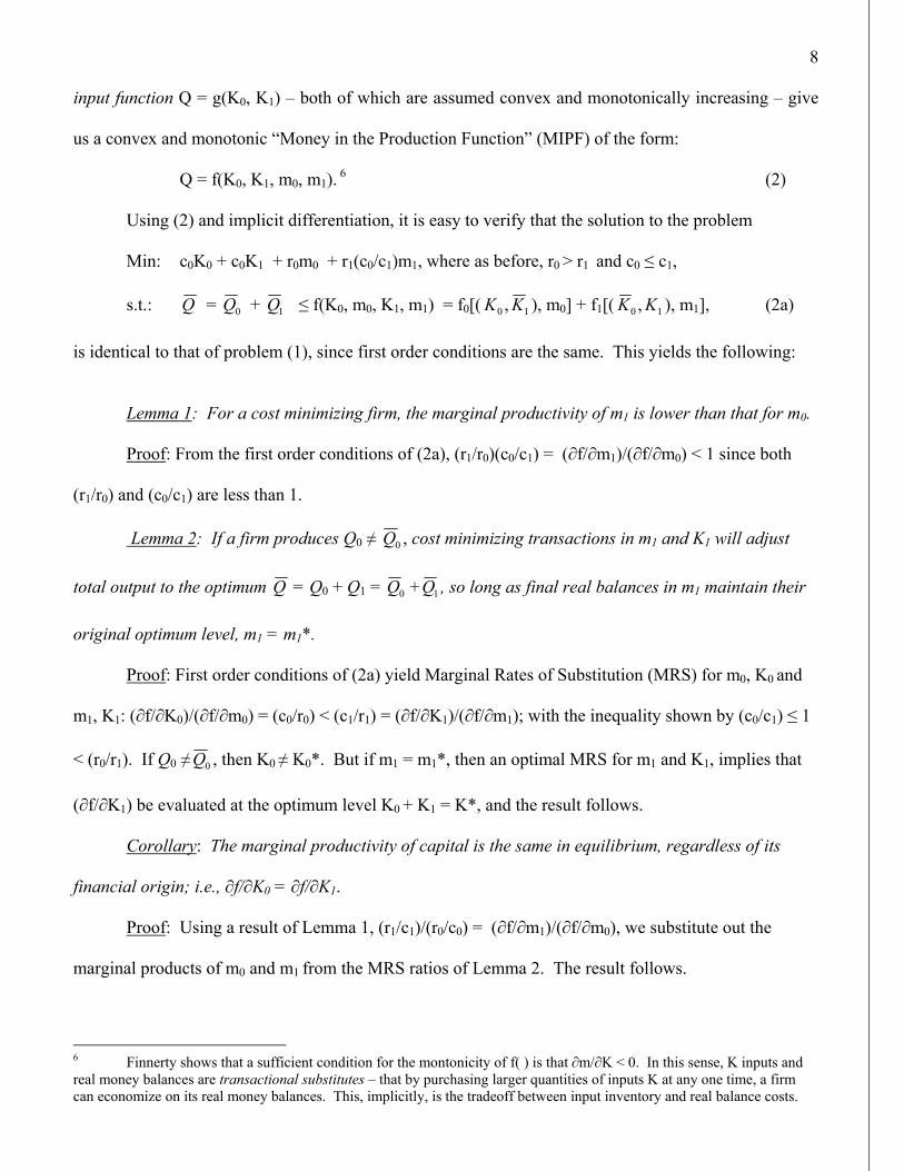
8
input function Q = g(K0, K1) – both of which are assumed convex and monotonically increasing – give
us a convex and monotonic “Money in the Production Function” (MIPF) of the form:
Q = f(K0, K1, m0, m1). 6 (2)
Using (2) and implicit differentiation, it is easy to verify that the solution to the problem
Min: c0K0 + c0K1 + r0m0 + r1(c0/c1)m1, where as before, r0 > r1 and c0 ≤ c1,
s.t.: Q = 0Q + 1Q ≤ f(K0, m0, K1, m1) = f0[( 10 , KK ), m0] + f1[( 10 , KK ), m1], (2a)
is identical to that of problem (1), since first order conditions are the same. This yields the following:
Lemma 1: For a cost minimizing firm, the marginal productivity of m1 is lower than that for m0. Proof: From the first order conditions of (2a), (r1/r0)(c0/c1) = (∂f/∂m1)/(∂f/∂m0) < 1 since both
(r1/r0) and (c0/c1) are less than 1.
Lemma 2: If a firm produces Q0 ≠ 0Q , cost minimizing transactions in m1 and K1 will adjust
total output to the optimum Q = Q0 + Q1 = 0Q + 1Q , so long as final real balances in m1 maintain their
original optimum level, m1 = m1*.
Proof: First order conditions of (2a) yield Marginal Rates of Substitution (MRS) for m0, K0 and
m1, K1: (∂f/∂K0)/(∂f/∂m0) = (c0/r0) < (c1/r1) = (∂f/∂K1)/(∂f/∂m1); with the inequality shown by (c0/c1) ≤ 1
< (r0/r1). If Q0 ≠ 0Q , then K0 ≠ K0*. But if m1 = m1*, then an optimal MRS for m1 and K1, implies that
(∂f/∂K1) be evaluated at the optimum level K0 + K1 = K*, and the result follows.
Corollary: The marginal productivity of capital is the same in equilibrium, regardless of its
financial origin; i.e., ∂f/∂K0 = ∂f/∂K1.
Proof: Using a result of Lemma 1, (r1/c1)/(r0/c0) = (∂f/∂m1)/(∂f/∂m0), we substitute out the
marginal products of m0 and m1 from the MRS ratios of Lemma 2. The result follows.
6 Finnerty shows that a sufficient condition for the montonicity of f( ) is that ∂m/∂K < 0. In this sense, K inputs and real money balances are transactional substitutes – that by purchasing larger quantities of inputs K at any one time, a firm can economize on its real money balances. This, implicitly, is the tradeoff between input inventory and real balance costs.
9
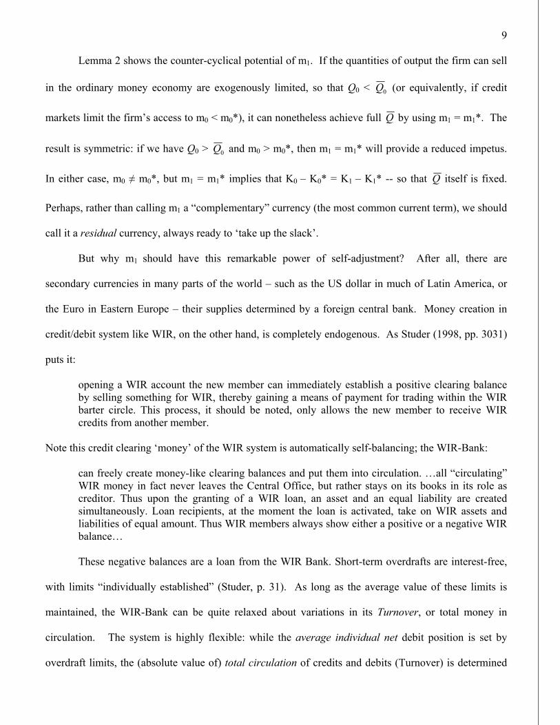
Lemma 2 shows the counter-cyclical potential of m1. If the quantities of output the firm can sell
in the ordinary money economy are exogenously limited, so that Q0 < 0Q (or equivalently, if credit
markets limit the firm’s access to m0 < m0*), it can nonetheless achieve full Q by using m1 = m1*. The
result is symmetric: if we have Q0 > 0Q and m0 > m0*, then m1 = m1* will provide a reduced impetus.
In either case, m0 ≠ m0*, but m1 = m1* implies that K0 – K0* = K1 – K1* -- so that Q itself is fixed.
Perhaps, rather than calling m1 a “complementary” currency (the most common current term), we should
call it a residual currency, always ready to ‘take up the slack’.
But why m1 should have this remarkable power of self-adjustment? After all, there are
secondary currencies in many parts of the world – such as the US dollar in much of Latin America, or
the Euro in Eastern Europe – their supplies determined by a foreign central bank. Money creation in
credit/debit system like WIR, on the other hand, is completely endogenous. As Studer (1998, pp. 3031)
puts it:
opening a WIR account the new member can immediately establish a positive clearing balance by selling something for WIR, thereby gaining a means of payment for trading within the WIR barter circle. This process, it should be noted, only allows the new member to receive WIR credits from another member.
Note this credit clearing ‘money’ of the WIR system is automatically self-balancing; the WIR-Bank:
can freely create money-like clearing balances and put them into circulation. …all “circulating” WIR money in fact never leaves the Central Office, but rather stays on its books in its role as creditor. Thus upon the granting of a WIR loan, an asset and an equal liability are created simultaneously. Loan recipients, at the moment the loan is activated, take on WIR assets and liabilities of equal amount. Thus WIR members always show either a positive or a negative WIR balance… These negative balances are a loan from the WIR Bank. Short-term overdrafts are interest-free,
with limits “individually established” (Studer, p. 31). As long as the average value of these limits is
maintained, the WIR-Bank can be quite relaxed about variations in its Turnover, or total money in
circulation. The system is highly flexible: while the average individual net debit position is set by
overdraft limits, the (absolute value of) total circulation of credits and debits (Turnover) is determined

10
only by economic need. The net of this total, meanwhile, is identically zero due to “the automatic plus-
minus balance of the system as a whole” (Studer, p. 31) – a practical confirmation of Say’s Law, also an
identity (Clower and Howitt, 1998). It is this balanced credit flexibility – neither inflationary nor
deflationary, as long as overdraft limits are maintained – that forms the promise of what Studer (p. 31)
calls “practically unlimited potential” for expansion under a centralized barter system.7
III.2 Empirical Specifications
The counter-cyclical element of our residual currency is not its m1 balances, which Lemma 2
shows to be quite stable. It is rather m1 Turnover, or total WIR-money in circulation – essentially the
WIR-net-credit balances times their velocity. From (1a) and (2a), define Turnover as 1~m = c1K1 = c1(K*
- K0), with a dominant currency value of (c0/c1) 1~m = (c0/c1)c1K1 = c0K1. Since the WIR-Bank keeps
track of this Turnover, we can estimate its correlation with GDP and Unemployment.
If 1~m = c1K1 = c1(K* - K0), there is a clear counter-cyclical implication. That is, if full potential
output Q = g(K0, K1) is not reached, then both 1~m (Turnover) and 1
~m /m1 (Velocity) should be:
o inversely correlated with variation in output Q (below, GDP), o inversely correlated with variation in broad money supply m0 (below, M2), and o directly correlated with variation in the number of unemployed (below, UE)
– all in the short-term. In the longer term, if WIR’s share of the financial system (m1/m0) is fairly stable,
then m0, m1, and Turnover 1~m should all grow along with Swiss GDP. This distinction between short
term and long term variation suggests an Error-Correction Model (ECM) specification.
As will be seen, there is strong evidence for Granger causality of the broad Swiss money supply
measure M2 upon GDP and upon WIR-Turnover – but not vice-versa. This makes sense in terms of our
model, since variations in Turnover 1~m are driven by variations in m0 –not vice-versa. It is also
probably due to the small amounts of WIR in the Swiss national economy. Swiss M2 measured 475.1
7 The remarkable flexibility of an “automatic plus-minus balance” system is also shown in a pedagogical experiment designed by LETS founder Michael Linton (2007), available at www.openmoney.org/letsplay/index.html.

11
Billion Swiss Francs (SFr) in 2003,8 whereas annual Turnover in WIR is seen in Table 1 to have been
1.65 Billion SFr that same year. Thus the ratio of WIR Turnover to M2 is only one third of one percent.
In our MIPF formalization (2a), what signs do we expect on the derivatives of m0 and m1? Due
to the limitation on exchange to the Wirtschaftsring; i.e., among members of the reciprocal exchange
community, m1 will of course be less fungible. Lemma 1 shows that m1 will also be less transactionally
productive than m0 in realizing Q in the long run. That is, in the ECM portions of our specifications,
for the effect of the terms m0, m1, and 1~m (i.e., M2 money supply, WIR Credit balances, and WIR
Turnover, respectively) upon GDP:
0~f
mf
mf
110
>∂∂
>∂∂
>∂∂
m (3)
In many MIPF estimates (not shown here), there is clear evidence for the positive signs in (3). Evidence
for their relative ordering, however, is mixed.
By the substitutability of m0 and m1 shown in Lemma 2, these terms should be negatively
correlated in the short-term or cyclical sense: om~ – *0
~m = 1~m – *
1~m . Numerous estimates (also not shown)
show that m0 and m1 are pro-cyclical. This is not at all surprising: the pro-cyclical character of the
normal money supply is well known (Mankiw, 1993; Mankiw and Summers, 1993; Bernanke and
Gertler, 1995; Gavin and Kydland, 1999). We will concentrate our presentation on the estimates that
show 1~m (“Turnover”) is counter-cyclical.
From our result on Turnover we have 1~m = c1K1 = c1(K* - K0), so that ∂ 1
~m /∂K0 = -c1 < 0. Since
K0 in our model varies directly with m0 and Q0 (the overwhelming bulk of output), and indirectly with
unemployment in the short term, we expect to find some short term partial derivatives of the form:
∂ 1~m /∂Q < 0, (4.1)
∂ 1~m /∂m0 < 0, and (4.2)
8 Swiss National Bank (SNB) Monthly Statistical Bulletin (August 2005), Table B2, Monetary aggregates: www.snb.ch/e/publikationen/publi.html?file=/e/publikationen/monatsheft/aktuelle_publikation/html/e/inhaltsverzeichnis.html
12
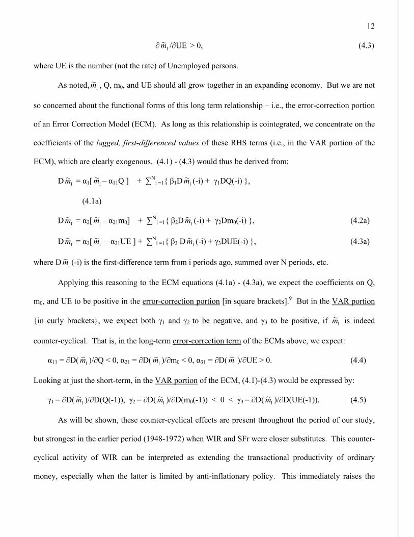
∂ 1~m /∂UE > 0, (4.3)
where UE is the number (not the rate) of Unemployed persons.
As noted, 1~m , Q, m0, and UE should all grow together in an expanding economy. But we are not
so concerned about the functional forms of this long term relationship – i.e., the error-correction portion
of an Error Correction Model (ECM). As long as this relationship is cointegrated, we concentrate on the
coefficients of the lagged, first-differenced values of these RHS terms (i.e., in the VAR portion of the
ECM), which are clearly exogenous. (4.1) - (4.3) would thus be derived from:
D 1~m = α1[ 1
~m – α11Q ] + ∑Ni =1{ β1D 1
~m (-i) + γ1DQ(-i) },
(4.1a)
D 1~m = α2[ 1
~m – α21m0] + ∑Ni =1{ β2D 1
~m (-i) + γ2Dm0(-i) }, (4.2a)
D 1~m = α3[ 1
~m – α31UE ] + ∑Ni =1{ β3 D 1
~m (-i) + γ3DUE(-i) }, (4.3a)
where D 1~m (-i) is the first-difference term from i periods ago, summed over N periods, etc.
Applying this reasoning to the ECM equations (4.1a) - (4.3a), we expect the coefficients on Q,
m0, and UE to be positive in the error-correction portion [in square brackets].9 But in the VAR portion
{in curly brackets}, we expect both γ1 and γ2 to be negative, and γ3 to be positive, if 1~m is indeed
counter-cyclical. That is, in the long-term error-correction term of the ECMs above, we expect:
α11 = ∂D( 1~m )/∂Q < 0, α21 = ∂D( 1
~m )/∂m0 < 0, α31 = ∂D( 1~m )/∂UE > 0. (4.4)
Looking at just the short-term, in the VAR portion of the ECM, (4.1)-(4.3) would be expressed by:
γ1 = ∂D( 1~m )/∂D(Q(-1)), γ2 = ∂D( 1
~m )/∂D(m0(-1)) < 0 < γ3 = ∂D( 1~m )/∂D(UE(-1)). (4.5)
As will be shown, these counter-cyclical effects are present throughout the period of our study,
but strongest in the earlier period (1948-1972) when WIR and SFr were closer substitutes. This counter-
cyclical activity of WIR can be interpreted as extending the transactional productivity of ordinary
money, especially when the latter is limited by anti-inflationary policy. This immediately raises the

13
question of whether such alternative-money activity is itself inflationary – a question to which I will
return in this paper’s conclusion.
IV. Empirical Results
IV.1. Data and Initial estimates
Because the WIR record is not widely available, I provide the basic data. The WIR bank has
provided 56 years of data on Nombre de Comptes-Participants (“Number of Account-Participants”),
Chiffre (o Volume) d'Affaires (“Turnover” activity), and Autres Obligations Financières envers Clients
en WIR (or “Credit” advanced in the form of credit to one’s reciprocal exchange account). Turnover and
Credit are equivalent to 1~m and m1 in our model, respectively, and are given in terms of WIR; i.e., their
Swiss Franc (SFr) equivalents. Other macro-economic time series used in this paper are from Madison
(1995), Mitchell (1998), OECD (2000), the IMF (2004) and World Bank (2004).
(Please Insert Table 1 about here.)
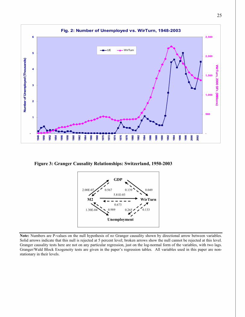
These data raise a number of questions. Consider Figure 2 below, which plots WIR Turnover
relative to the number of Unemployed in Switzerland:
1) What explains the turning points in WIR Turnover in the early 1970s, ‘80s, and -90s? 2) WIR Turnover tracks the number of Unemployed fairly closely. Is this evidence of a counter-
cyclical trend?
As will be seen in what follows, this paper may help explain a change in WIR trend in the early 1970s,
but not the later turning points. And we do find some evidence for a counter-cyclical trend.
(Please Insert Figure 2 about here.)
Estimates of the Swiss GDP production function (not shown here) were consistent with our basic
MIPF equation (2), when specified with inputs of Capital, Labor, and Money (M2). Furthermore, all
coefficients had the expected positive signs in most specifications of the underlying error-correction
equation, Q = f(L, K, m), and also in the VAR portion of the ECM.
9 Note that while α11, α21, α31 > 0, there is a negative sign placed before them in (4.1a - 4.3a).
14
IV.2. Effect of GDP upon WIR Turnover
Our estimates of equation (4.1a) in Table 2 below show that lagged GDP has the expected
positive sign in the error correction component of each regression, with cointegration significant in 2(A),
but not 2(B).10 The latter is also problematic because there is evidence of serial correlation. Granger/
Exogeneity tests are at or near 5 percent significance in both columns. In the VAR portions of the
regressions, coefficients on the first lag of differenced GDP, and also the lag of the first-differenced 2-
year growth term have the expected negative (counter-cyclical) sign. Coefficients on first lagged
difference term in 2(A) are comparable in absolute value to the coefficients on the second lag – so that
the net effect appears minimal. Since we are concerned with short-term stabilization, however, this is
not problematic.
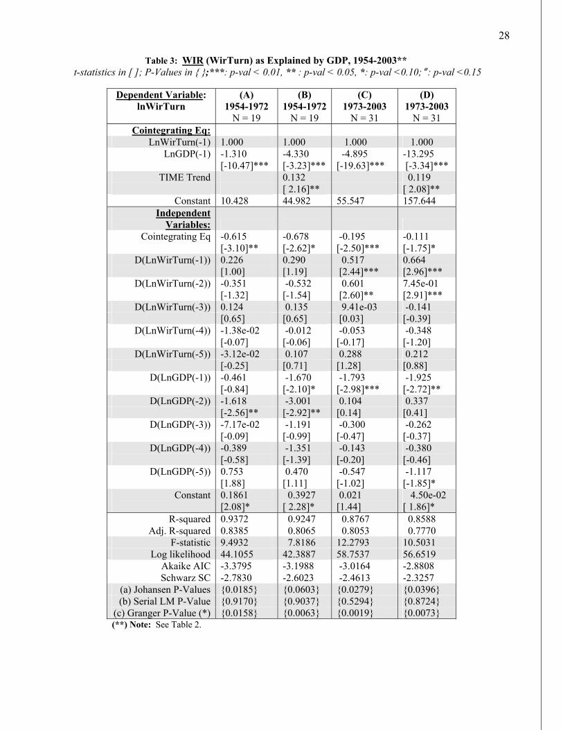
(Please insert Table 2 and Table 3 about here.)
Table 3 shows evidence of a structural break in the relationship between GDP and WIR
Turnover. Rejoining the time series of columns 3(A) and 3(C) for a single regression, we find P-values
of 2.55e-06 and 1.17e-03 for the Chi-Squared statistic of the Chow Breakpoint and Forecast tests,
respectively. Similarly joining up 3(B) and 3(D), we find Breakpoint and Forecast P-values of 2.98e-06
and 1.29e-03, respectively. What could cause such a structural break around 1973?
According to official histories, Defila (1994) and Studer (1998), 1973 was a turning point for the
WIR-Bank. A conflict arose over the widespread “discounting” of WIR – unused credits sold directly
for SFr, usually at substantial discount. WIR introduced measures to detect and prohibit such trading in
the fall of 1973. Of course WIR will usually be worth less than SFr in direct trade, since it cannot be
used as widely. Studer reports (1988, p. 21) that a counter-cyclical monetary argument was raised to
defend this discount trade: “that it created additional turnover and facilitated members’ ability to ride out
periodic currency-liquidity bottlenecks.” Table 3 shows that these arguments may have had a point.
10 Recall that the coefficients in the estimated error-correction form are negatives of those in the underlying equation.

15
There are other events, besides the ban on “discounting,” which could have caused a structural
break in this series, and which might also be expressed by changes in the cost of carrying out
transactions in m0 and m1. From Figure 4 below, some of the turning points in the volume in WIR
turnover, in the early 1970s, ‘80s, and ‘90s, appear to coincide with contrary changes in the value of the
Swiss Frank. Our initial regressions did not support this conjecture, but it remains plausible.11, 12
Note that in the underlying cointegrating equations of Table 3, WIR is positively correlated with
GDP, both pre-1973 and post-1973, as in inequality (4.4). But the significance and size of the
coefficients on the error-correction term are much greater pre-1973: greater in 3(A) than 3(C), and in
3(B) than 3(D).
In the pre-1973 estimates of columns 3(A) and (B), the VAR coefficients on the first two lags of
differenced GDP are both negative and counter-cyclical, as in (4.5) – and significant except for the first
lag in 4(A). In the post-1973 columns 3(C) and (D), by contrast, only the first lagged terms are
negative. Importantly, the sum of the first two periods’ lags is both greater and more significant pre-
1973. Thus, compare column 3(A): (sum = -2.08, p-value = 0.024) versus 3(C): (sum = -1.69, p-value =
0.111), and column 3(B): (sum = -4.67, p-value = 0.018) versus 3(D): (sum = -1.59, p-value = 0.209).13
The Granger/exogeneity tests in Table 3 are also highly significant, most at the 1 percent level.
GDP clearly Granger-causes WIR in both periods, but this causation can be shown to also be reciprocal
in the later period. Granger causality is even more significant in the ‘reverse’ WIR-to-GDP direction,
with P-values of 2.84e-05 in 3(C) and 1.17e-05 in 3(D). This movement from one-way to two-way
11 The negative correlation between Swiss Franc’s foreign exchange rate and WIR Turnover is quite strong for the periods 1970-75, 1980-85, and 1993-96 – around three significant turning points for the WIR series (IMF, 2007). Even the identification of a structural break in 1973, however, does not tell us what caused that break. There were many big changes in the world economy around that time: collapse of the Bretton Woods agreements, devaluation of the US dollar, the formation of OPEC, high levels of inflation, negative real interest rates, growth of the Eurodollar market, and the increasing ‘disintermediation’ of traditional financial institutions. All of these may plausibly be modeled as a higher r0, the opportunity cost for holding Swiss Franks – and thus a reduced counter-cyclical role for m1. 12 1973 is not even the only structural break that may be identified over this period. It can be shown that 1976 is also a significant break for the data underlying Table 4, under both Chow tests. 13 Standard error terms for these summation terms are calculated from the covariance matrix of the lagged terms.
16
causality flows is further evidence of a structural change. To repeat, however, WIR has never been
large enough to be an important determinant of Swiss GDP.
IV.3. The Effect of Unemployment Upon WIR Turnover
As Figure 2 above has already shown, growth in the number of Swiss Unemployed workers
tracks the number of WIR Participants very closely, with the former about ten times as large in
percentage change as the latter. This importance of Unemployment to WIR's trend probably reflects its
exclusion of "large" businesses, another important change in the bank's rules since 1973 (Defila 1994).
Employees in smaller, less diversified firms have less human capital accumulated, and are much more
subject to unemployment risk in many countries, including Switzerland (Winter-Ebmer and Zweimüller
1999, Winter-Ebmer 2001). Smaller firms also typically have more restricted access to formal credit
institutions (Terra, 2003), and their owners must rely proportionately more on self-financing, which also
increases their risk exposure (Small Business Administration, 1998).
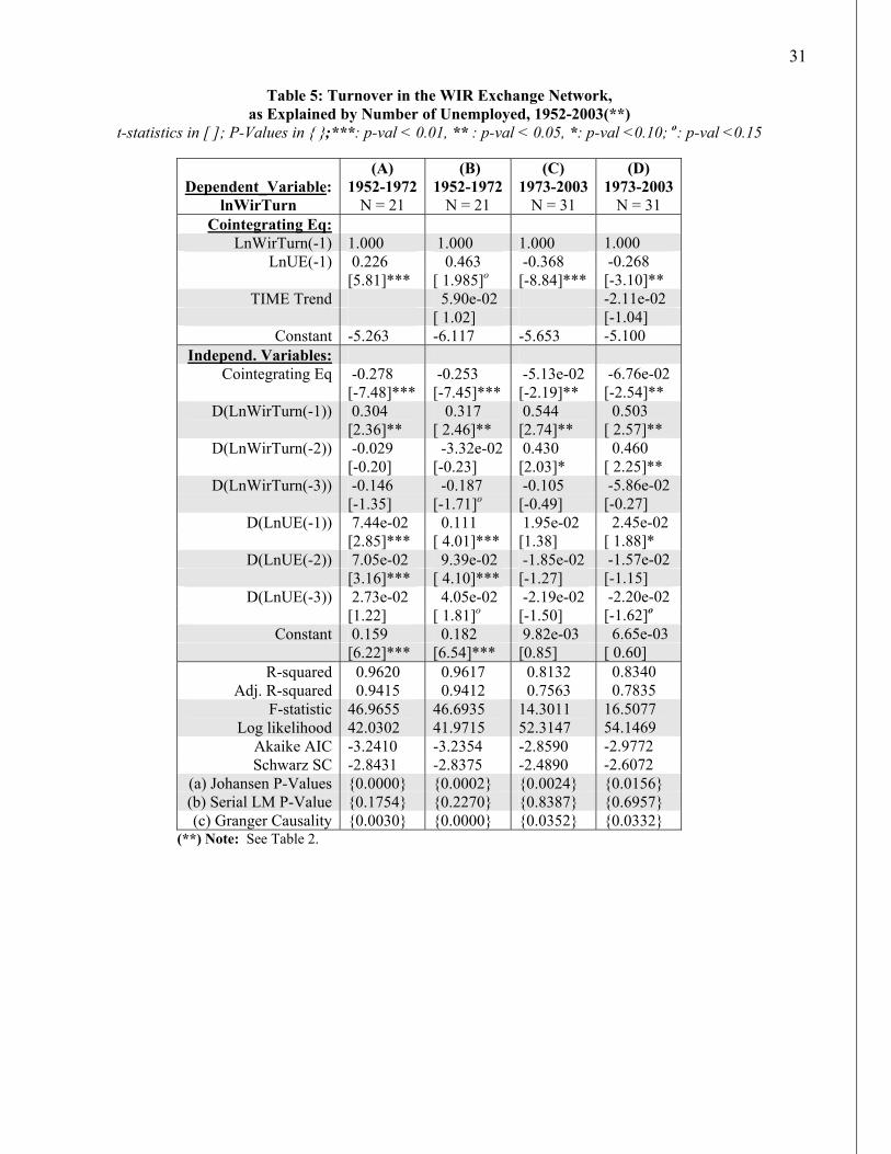
From ECM estimations on these data, it can be shown that the long-term (“secular”) cointegrated
relationship between WIR Accounts and the Number of Unemployed Workers is positive, as in
inequality (4.4). The short-term (“cyclical”) effect of Unemployment upon WIR Turnover – lagged
differences in the VAR portion – is highly counter-cyclical over the period 1949-2003, as seen in Table
4. Note that correlation between lagged changes in Unemployment and Turnover is positive and
counter-cyclical, consistent with inequality (4.5).
(Please insert Table 4 and Table 5 about here.)
Similarly to the previous regressions on GDP, the relationship of Turnover to Unemployment
can be shown to undergo a structural break around 1973, and become less counter-cyclical thereafter.
This is true, even though the counter-cyclical relationship is relatively strong over the entire period
1945-2003.
If we run a single regression over the entire 1954-2003 period split by the regressions in columns
5(A) and (C), the Chow Breakpoint and the Chow Forecast Chi-squared tests give contradictory results

17
on the null hypothesis of no structural break: the Chow Breakpoint fails to reject this null, with a rather
high P-value of 0.144; the Chow Forecast test rejects it decisively with a P-value of 1.26e-03. 14
However, if we regress over the entire period split by regressions 5(B) and (D), including their time
trend, the Chow Breakpoint test has a P-value of 6.73e-03, and similarly, the Chow Forecast test a P-
value of 9.06e-09.
Counter-cyclical effects are far stronger pre-1973, in columns 5(A) and (B), than post-1973, in
columns 5(C) and (D). The coefficients on lagged, first-differenced UE in 5(A) and (B) are also more
significant, and for two periods instead of just for one, as in 5(C) and (D). Note the size of coefficients
on the error correction terms are also greater pre-1973, by 4 or 5 times, and more significant by several
orders of magnitude. This is similar to the period contrast for our regression on GDP, in Table 3.
Also as in Table 3, Granger-causality in Table 4 is reciprocal for the later, but not the earlier
period. P-values for the opposite direction – for WIR Granger-causing Unemployment – were 0.1587
and 0.1343 for columns 5(A) and (B), but 0.0408 and 0.0369 on columns 5(C) and (D), respectively.
Again, it is unlikely that WIR, of small value within the Swiss national economy, could directly cause
significant changes in the number of unemployed persons. But again, this change in the directions of
Granger causality does suggest some basic structural shift.
IV.4. The Effect of M2 Upon WIR Turnover
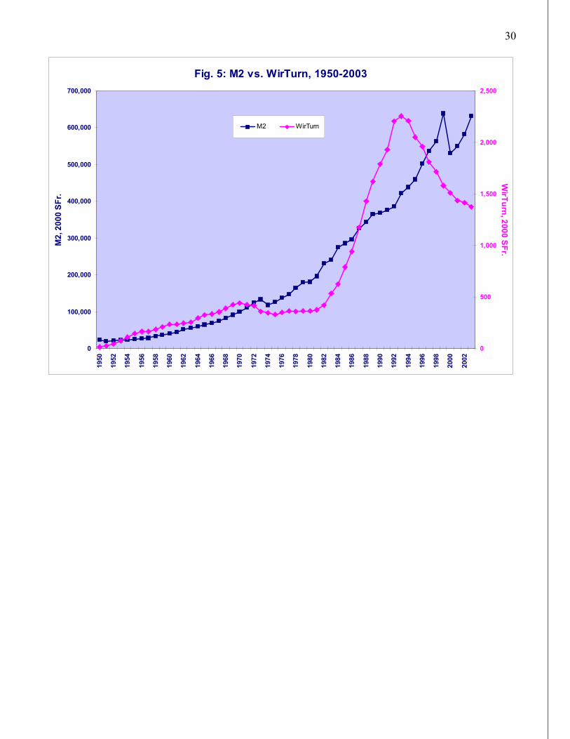
We next come to an obvious question: If WIR became less tradable for Swiss Francs after 1973,
what happened to the correlation between WIR and the Swiss money supply? Figure 5 suggests that
WIR followed Swiss M2 very closely up to about 1972, but seems to have “decoupled” since then.
(Please insert Figure 5 about here.)
Chow Chi-squared tests give clear confirmation of a structural break in the relation between WIR
and SFr. in 1973. For a single regression over the entire period split between regressions 6(A) and (C),
14 It is not unusual for the two Chow tests to yield qualitatively different results. While the Chow Breakpoint test on this form does not meet standard significance, other evidence of structural change in the Table 5 is strong, and consistent with the Chow Forecast test.

18
the Breakpoint test shows structural change significant at 1.62e-02, the Forecast test at 1.08e-04. For a
single regression uniting the period of 6(B) and (D), and the Chow Breakpoint test shows a structural
break is significant at 3.98e-03, the Forecast test at 9.94e-05.
All the error correction components in Table 6 show significant positive correlation between M2
and WIR, as one would expect in a growing economy. It appears that M2 was much more closely tied to
WIR before 1973 in the long-term, secular, cointegrated sense. As in our previous Tables 3 and 5, the
coefficient on the error correction term is larger and more significant in the earlier pre-1973 period.
Here, comparing columns 6(B) and (D), the coefficient on M2 in the error correction component of 6(B)
is an order of magnitude greater than in 6(D). Interpreted as long-run elasticities, a permanent one
percent rise in M2 before 1973 would increase WIR-Turnover by over 70 percent in the long-term.
Post-1973, by contrast, the long-term change in WIR-Turnover would be less than 7 percent. We note
that the trended specification of ECM in columns 6(B) and (D) is more reliable, since the specification
in 6(A) and (C) fails to show Granger causality, and also because 6(C) shows no cointegration.15
In contrast to the closer long-run relationship in the earlier period, however, the short term
elasticities are more negative, more significant, and more persistent post-1973. Examining the short
term coefficients in the VAR portion of columns 6(B) and (D), we see that the latter set are higher in
absolute value for the first two lags, and more significant for three lags. The “decoupling” of WIR and
M2 seen in Figure 5 can thus be seen as a combination of these two effects – a greater positive long-run
elasticity pre-1973, and more negative short-run elasticity post-1973. The negativity of the short-run
effect makes sense in our model, which shows 1~m counter-cyclical to the pro-cyclical m0, in (4.5). Our
model does not explain, however, why these coefficients should appear more negative post-1973.
(Please insert Table 6 about here.)
15 Note that, as in our previous Tables 3 and 5, Granger causality can also flow in the reverse direction post-1973, column (D) showing a reverse causality significant at the 1 percent level.

19
V. Conclusions and Discussion This linkage between WIR and M2 begs the question – which was more effective as a counter-
cyclical tool? There is clear evidence of M2’s pro-cyclical performance (not shown here) for the entire
period 1952-2003. This is consistent with our theory, which shows that short term variation in m0 can
be pro-cyclical. And it is reinforced by a considerable literature (Mankiw, 1993; Mankiw and Summers,
1993; Bernanke and Gertler, 1995; Gavin and Kydland, 1999) finding that the broad money supply is
highly pro-cyclical. Even less controversial is the finding that the velocity of money is pro-cyclical
(Tobin 1970, Goldberg and Thurston 1977, Leão 2005). Our key variable, WIR Turnover, is actually
WIR-money times Velocity, so the counter-cyclical trend of WIR Turnover (pre-1973) is doubly
impressive.16
Our estimates suggest that WIR-Bank’s creation of purchasing power could become an
instrument of macro-economic policy. According to our model, furthermore, this result is not highly
scale-dependent. (Recall that by our latest data, in 2003 WIR-Turnover/M2 = 0.35%.) Rather, it is a
result of the automatic net-zero balance system like WIR (Studer, p. 31).
There is substantial evidence for the general form of our hypothesis, that centralized reciprocal
exchange of WIR is counter-cyclical with GDP, and even more so with the Number of Unemployed.
These results may help answer a basic question within macroeconomic theory – whether macro-
instability is more due to price rigidity, or to instability in money and credit. Keynes (1936) recognized
that both conditions can apply, and that either can lead to instability. Macroeconomists like Colander
(1996, 2006) stress monetary and credit conditions. The consensus, however, as represented by Mankiw
(1993), puts the blame more on rigid prices. Our model clearly supports the monetary side, focusing on
“wrong” levels of M2 – which can be smoothed over by variations in WIR Turnover.
16 Further regressions (not shown here) show that WIR velocity is in fact highly counter-cyclical, while WIR credits are themselves somewhat pro-cyclical. The net effect on Turnover is counter cyclical.
20
Reflecting the macroeconomic consensus, most commentary on e-commerce has stressed its
improved price flexibility.17 However, telecommunications networks show increasing returns to scale
(Romer 1997, Howitt and Phillipe 1998, Arthur 1996), and this may fuel pro-cyclical instability. This is
the implication of several recent models and simulations (Azariadis and Chakraborty, 1998;
Chichilnisky and Gorbachev, 2004; Sterman et. al., 2006). The WIR exchange network is also subject
to increasing returns and "network externalities," yet its activity appears counter-cyclical.
What about the inflationary potential of such a network? A preliminary observation is that at
current scale, it is unlikely to have any measurable effect. More theoretically interesting points are
worth considering, however.
First, since WIR Turnover is counter-cyclical and M2 turnover is pro-cyclical, changes in WIR
should be less inflationary than those in M2 itself.
Second, if net Credit limits are stable, the automatic net balancing of WIR Turnover, with new
credits matched by new debits, allows short-term fluctuations in real output to be matched by velocity.
This is potentially consistent with price neutrality. In terms of the quantity equation (for the WIR
system itself), Turnover = MV = PY. If M (money) is unchanged, and if any change in V (velocity) is
matched by a change in Y (real goods and services), then the change in P (price) must be zero: If ∆M =
0 and ∆V = ∆Y, then ∆P = 0. This “practically unlimited potential” (Studer, p. 31) for self-balancing
credit creation would only be strictly true for a closed WIR-type system, however.
In fact, however, and as our final point, WIR is a counter-cyclical “residual” currency. Our
estimates show that it is most likely to be accepted when ordinary (pro-cyclical) money is in short
supply. This should focus the transactional effectiveness of WIR – to be greatest precisely where its
17 Magenheim and Murrell (1988) see the persistence of barter as explained by its lack of transparency, providing greater scope for price discrimination. The WIR record does not record support this hypothesis, however since: (a) WIR activities are often advertised and always centrally recorded – and thus inappropriate for “confidential” price discrimination. (b) As previously noted, prices for goods and services advertised in WIRPlus (2000-2005) are often higher in WIR than in Swiss Francs, so this is not obviously downward price flexibility. (c) WIR's bylaws restrict membership to small and medium businesses (Defila 1994), and these will have little price-setting power. Thus, while the Magenheim-Murrell (1988) may hold for other forms of ‘countertrade’, WIR’s counter-cyclical trend is not likely to stem from improved price flexibility.

21
inflationary potential is the least. WIR money does not ‘top up’ the supply of Swiss Francs – it
substitutes for Swiss Francs that are otherwise unavailable. The effect of increased WIR Turnover on
prices is not inflationary, then, but anti-deflationary.
References ARTHUR, W. Brian (1996) “Increasing Returns and the New World of Business”, Harvard Business Review, Boston: July-August. AZARIADIS, Costas, and Shankha Chakraborty (1998) “Asset Price Volatility In A Nonconvex General Equilibrium Model,” Journal of Economic Theory, (12)3, pp. 649-665. BEATTIE, Alan (1999) "Internet Heralds Coincidence of wants," Financial Times, Dec. 6. BERNANKE, Ben S. and Gertler, Mark (1995) “Inside the Black Box: The Credit Channel of Monetary Policy Transmission,” Journal of Economic Perspectives; Fall 1995, 9(4), p. 27 48. CHICHILNISKY, Graciela, and Olga Gorbachev (2004) “Volatility in the Knowledge Economy”, Journal of Economic Theory, (24)3, (Oct.), pp. 531-47. CLOWER, Robert and Peter HOWITT (1998) “Keynes and the Classics: An End of Century View, in Keynes and the
Classics Reconsidered, Ahiakpor, James C. W. (ed.), Boston: Kluwer Academic Press. CALVO, Guillermo, and Carlos Végh (1992) “Currency Substitution In Developing Countries: An Introduction,” IMF Working Paper 92/40 (May 1992). COLACELLI, Mariana, and David J.H. Blackburn (2006) “Secondary Currency: An Empirical Analysis,” Columbia University, www.columbia.edu/~mc2602/files/Colacelli-Currency-Dec-06.pdf. COLANDER, David (2006), ed., Post Walrasian Macroeconomics: Beyond the Dynamic Stochastic General Equilibrium Model. Cambridge, UK: Cambridge University Press. ________________ (1996), ed., Beyond Micro-foundations: Post Walrasian Macroeconomics. Cambridge, UK: Cambridge University Press. CRAIG, Ben. R, and Christopher J. Waller (2000) “Dual-Currency Economies as Multiple-Payment Systems,” Cleveland Federal Reserve, Economic Review, Quart. 1, 36(1), pp. 2-13. http://clevelandfed.org/research/review/2000/index.cfm#Q1 CURTIS, Elisabeth S., and Christopher J. Waller (2000) “A Search-Theoretic Model of Legal and Illegal Currency,” Journal of Monetary Economics, 45(1), February, pp. 155–84. DAVIES, Glyn (1994) A History of Money, Cardiff, UK: University of Wales Press. DEFILA, Heidi (1994) "Sixty Years of the WIR Economic Circle Cooperative: Origins and Ideology of the Wirtschafts- ring," WIR Magazin, September. (Translation by Thomas Geco.) http://www.ex.ac.uk/~RDavies/arian/wir.html. Economic Report of the President (1996), Washington, DC: US Government Printing Office. Economist Magazine (2000a), "Economics Focus: Who Needs Money?" January 22. _________________ (2000b), "Economics Focus: E-Money Revisited," July 22. ECKALBAR, John,C. (1984) "Money, Barter and Convergence to the Competitive Allocation: Menger's Problem",
Journal of Economic Theory, 32, April: 201-11. FEENSTRA, Robert C., (1986) “Functional Equivalence between Liquidity Costs and the Utility of Money,” Journal of
Monetary Economics, Vol. 17, pp 271-291. FINNERTY, John (1980) “Real Money Balances and the Firm's Production Function: A Note,” Journal of Money, Credit, and Banking, 12(4) November, Part 1: 666-71. FEIGE, Edgar L. (2003) "The Dynamics of Currency Substitution, Asset Substitution and De Facto Dollarization and Euroization in Transition Countries," Comparative Economic Studies, Fall, 2003. FISCHER, Stanley (1979) “Capital Accumulation on the Transition Path in a Monetary Optimizing Model,” Econometrica, 47(6), November, pp. 1433-40 _______________ (1974) "Money and the Production Function," Economic Inquiry, 12, December, pp. 517-33. FISHER, Irving (1934) Mastering the Crisis - With Additional Chapters on Stamp Scrip, Kimble & Bradford, London. FRIEDMAN, Benjamin (1999) "The Future of Monetary Policy", International Finance, December. GAVIN, William T. & Finn E. Kydland (1999) "Endogenous Money Supply and the Business Cycle," IB, Elsevier for the Society for Economic Dynamics, 2(2), April, pp. 347-369. GREENSPAN, Alan (1999) "Testimony before the Joint Economic Committee," US Congress, June 14. GOLDBERG, Matthew & Thurston, Thomas B. (1977) "Monetarism, Overshooting, and the Procyclical Movement of Velocity," Economic Inquiry, Oxford University Press, January, 15(1), pp. 26-32. GOMEZ, Georgiana M. (2006) “Our market, our community, our money. Complementary Currency Systems in Argentina,” Working paper. www.iss.nl/iss/profile/394. HANDA, Jagdish (2000) Monetary Economics, Routledge.
22
HASAN, M. Aynul ; Syed F. Mahmud (1993) “Is Money an Omitted Variable in the Production Function? Some Further Results,” Empirical Economics, 18(3) (1993): 431-45. INTERNATIOANL MONETARY FUND (IMF), International Financial Statistics, http://imfstatistics.org. KING, Mervyn (1999) "Challenges for Monetary Policy: New and Old." Paper prepared for the Symposium on “New Challenges for Monetary Policy” sponsored by the Federal Reserve Bank of Kansas City at Jackson Hole, Wyoming, 27 August 1999. www.bankofengland.co.uk/speeches/speech51.pdf . KEYNES, John Maynard (1936) The General Theory of Employment, Interest, and Money. New York: Harcourt Brace Jovanovich, 1964. LEÃO, Pedro (2005) “Why does the velocity of money move pro-cyclically?” International Review of Applied Economics, 19(1) January, pp. 119-135. LIETAER, Bernard (2004) “Complementary Currencies in Japan Today: History, Originality and Relevance,”
International Journal of Community Currency Research, Vol. 8, www.le.ac.uk/ulmc/ijccr/vol7-10/8toc.htm. LINTON, Michael (2007) “LETSplay” simulation of a WIR-type system, www.openmoney.org/letsplay/index.html. MADISON, Angus (1995) Monitoring the World Economy, 1820-1992, Paris: OECD. MAGENHEIM, E. and P. MURRELL (1988) "How to Haggle and Stay Firm: Barter as Hidden Price Discrimination" Economic Inquiry, July, Vol. 26, no.3. MANKIW, N. (1993) editor of “Symposium on Keynesian Economic Theory Today,” Journal of Economic Perspectives, Vol. 7, no. 1. MANKIW, N. and SUMMERS, L. (1993) “Money Demand and the Effects of Fiscal Policies” Journal of Money Credit
and Banking, Vol. 18, No. 4 (Nov., 1986), pp. 415-429 MIEIERHOFER, L. (1984) Volkswirtsaftliche Analyse des WIR-Wirtschaftsrings, WIR: Basel, Switzerland. MITCHELL, B.R. (1998) International Historical Statistics, Europe, 1750-1993, UK: MacMillan. OECD (2000) Economic Outlook, Jan., Paris: OECD. _____ (1999) Economic Surveys: Switzerland, Paris: OECD. _____ (1998) Main Economic Indicators, Historical Statistics, 1960-97 [computer file], Paris: OECD. ONIONS, C.T., (1966) Editor, The Oxford Dictionary of English Etymology, Oxford: Clarendon Press, 1995. PATINKIN, Don (1956) Money, Interest and Prices: An Integration of Monetary and Value Theory, Evanston, IL: Row, Peterson and Co. PLATNER, SAMUEL B. (1929), A Topographical Dictionary of Ancient Rome, London: Oxford University Press. POLANYI, Karl (1947) The Great Transformation: the political and economic origins of our time, Boston: Beacon Press, 1957. ROMER, Paul (1986) "Increasing Returns and Long-Run Growth," Journal of Political Economy Vol. 94, no. 5 (October): pp. 1002-37. RÖSL, Gerhard (2006) “Regional currencies in Germany – local competition for the Euro?” Discussion Paper, Series 1: Economic Studies No 43/2006, www.bundesbank.de/download/volkswirtschaft/dkp/2006/200643dkp_en.pdf SHORT, Eugenie D (1979) "A New Look at Real Money Balances as a Variable in the Production Function Journal of Money, Credit, and Banking, 11, August, pp. 326-39. SIDRAUSKI, Miguel (1967) ‘Rational Choice and Patterns of Growth in a Monetary Economy,” American Economic Review, Vol LVII, No 2, pp 534-544. SKIDELSKY, Robert (1992) John Maynard Keynes: The Economist as Savior, 1920-37, Vol. 2 of the author’s 3 part biography, New York: Penguin. SMALL BUSINESS ADMINISTRATION (1998) US Govt, “Financing Patterns of Small Firms: Findings from the 1998 Survey of Small Business Finance,” www.smallbusinessnotes.com/fedgovernment/sba/financingpatterns03.html.
STARR, Ross M., (ed.) (1989) General Equilibrium Models of Monetary Economies: Studies in the Static Foundations of Monetary Theory, San Diego: Academic Press. STERMAN, John, Rebecca M. Henderson, Eric D. Beinhocker, and Lee I. Newman, (February 2006). "Getting Big Too
Fast: Strategic Dynamics with Increasing Returns and Bounded Rationality" MIT Sloan Research Paper No. 4595-06: http://ssrn.com/abstract=886784
STODDER, James (1998) "Corporate Barter and Macroeconomic Stabilization," International Journal of Community Currency Research, Vol.2, http://www.le.ac.uk/ulmc/ijccr/vol1-3/2toc.htm. _____________ (1995) “The Evolution of Complexity in Primitive Economies: Theory,” and "…Empirical Evidence," Journal of Comparative Economics, Vol. 20: No. 1, February and No. 2, May. STUDER, Tobias (1998) WIR in Unserer Volkwirtschaft, Basel: WIR. An English translation of the non-statistical portion of this book is available as WIR and the Swiss National Economy (2006), translated by Philip H. Beard, Sonoma State University, Rohnert Park, California 94928. An E-Book version of this text is available at http://www.lulu.com/content/301348. The passages quoted in the present paper are taken from this translation. STUTZ, Emil (1984) "Le Cercle Économique-Societé Coopéreative WIR - Une Retrospective Historique," Basle: WIR. TERRA, Maria Cristina (2003) “Credit constraints in Brazilian firms: evidence from panel data.” Revista Brasilera de
Economia, Apr./June, vol.57, no.2, p.443-464.

23
TOBIN, James (1970) "Money and Income: Post Hoc Ergo Propter Hoc?," Quarterly Journal of Economics, MIT Press, May, 84(2), pp. 301-17.
WEITZMAN, Martin L (1982) “Increasing Returns and the Foundations of Unemployment Theory,” Economic Journal, 92(368), (Dec.), pp. 787-804. WENNINGER, John (1999) "Business-to-Business Electronic Commerce," Current Issues in Economics and Finance, June, Volume 5, no. 10. WINTER-EBMER, Rudolf, & Josef ZWEIMÜLLER (1999) “Firm Size Wage Differentials in Switzerland: Evidence from Job Changers,” American Economic Review, Papers and Proceedings, Vol. 89, No. 2, May, 89-93. WINTER-EBMER, Rudolf (2001) “Firm Size, Earnings, and Displacement Risk,” Economic Inquiry, Vol. 39, No. 3, July, pp. 474-486. WIR-Plus magazine, various issues, 2000-2007, www.wir.ch. WIR (2005) E-mail statistics from Office of Public Relations, December. WIR (2005) Rapport de Gestion, Various Years, Basle: WIR WORLD BANK (2004) World Development Indicators, www.worldbank.org/data/wdi2004/index.htm. ____________(2000) "Future of Monetary Policy and Banking Conference: Looking Ahead to the Next 25 Years," July 11, 2000, World Bank, www.worldbank.org/research/interest/confs/upcoming/papersjuly11/papjuly11.htm.

24
Table 1: Participants, Total Turnover, Credit, and Credit/Turnover, WIR-Bank, 1948-2003 (Total Turnover and Credit Denominated in Millions of Current Swiss Franks)
Year Participants Turnover Credit Year Participants Turnover Credit 1948 814 1.1 0.3 1976 23,172 223.0 82.2
1949 1,070 2.0 0.5 1977 23,929 233.2 84.5
1950 1,574 3.8 1.0 1978 24,479 240.4 86.5
1951 2,089 6.8 1.3 1979 24,191 247.5 89.0
1952 2,941 12.6 3.1 1980 24,227 255.3 94.1
1953 4,540 20.2 4.6 1981 24,501 275.2 103.3
1954 5,957 30.0 7.2 1982 26,040 330.0 127.7
1955 7,231 39.1 10.5 1983 28,418 432.3 159.6
1956 9,060 47.2 11.8 1984 31,330 523.0 200.9
1957 10,286 48.4 12.1 1985 34,353 673.0 242.7
1958 11,606 53.0 13.1 1986 38,012 826.0 292.5
1959 12,192 60.0 14.0 1987 42,227 1,065 359.3
1960 12,567 67.4 15.4 1988 46,895 1,329 437.3
1961 12,445 69.3 16.7 1989 51,349 1,553 525.7
1962 12,720 76.7 19.3 1990 56,309 1,788 612.5
1963 12,670 83.6 21.6 1991 62,958 2,047 731.7
1964 13,680 101.6 24.3 1992 70,465 2,404 829.8
1965 14,367 111.9 25.5 1993 76,618 2,521 892.3
1966 15,076 121.5 27.0 1994 79,766 2,509 904.1
1967 15,964 135.2 37.3 1995 81,516 2,355 890.6
1968 17,069 152.2 44.9 1996 82,558 2,262 869.8
1969 17,906 170.1 50.3 1997 82,793 2,085 843.6
1970 18,239 183.3 57.2 1998 82,751 1,976 807.7
1971 19,038 195.1 66.2 1999 82,487 1,833 788.7
1972 19,523 209.3 69.3 2000 81,719 1,774 786.9
1973 20,402 196.7 69.9 2001 80,227 1,708 791.5
1974 20,902 200.0 73.0 2002 78,505 1,691 791.5
1975 21,869 204.7 78.9 2003 77,668 1,650 784.4
Sources: Data to 1983 are from Meierhofer (1984). Subsequent years are from the annual Rapport de
Gestion and communications with the WIR public relations department (2000, 2005). The first three series (Participants, Turnover, and Credit) are given in the annual report in French as Nombre de Comptes-Participants, Chiffre (o Volume) d'Affaires, and Autres Obligations Financières envers Clients en WIR, respectively. Both Turnover and Credit are denominated in Swiss Francs, but the obligations they represent are payable in WIR-accounts. In the regressions, all WIR and monetary series are deflated by the 2000 GDP deflator. More recent data have not been made available.
25
Fig. 2: Number of Unemployed vs. WirTurn, 1948-2003
-
1
2
3
4
5
619
48
1950
1952
1954
1956
1958
1960
1962
1964
1966
1968
1970
1972
1974
1976
1978
1980
1982
1984
1986
1988
1990
1992
1994
1996
1998
2000
2002
Num
ber o
f Une
mpl
oyed
(Tho
usan
ds)
-
500
1,000
1,500
2,000
2,500
WirTurn, 2000 SFr. (M
illions)
UE WirTurn
Figure 3: Granger Causality Relationships: Switzerland, 1950-2003
GDP
2.00E-07 0.567 0.139 0.049_________5.81E-03
M2 WirTurn_____ ____0.673
1.30E-04 ____0.989 0.265 __0.133
Unemployment
Note: Numbers are P-values on the null hypothesis of no Granger causality shown by directional arrow between variables. Solid arrows indicate that this null is rejected at 5 percent level; broken arrows show the null cannot be rejected at this level. Granger causality tests here are not on any particular regression, just on the log-normal form of the variables, with two lags. Granger/Wald Block Exogeneity tests are given in the paper’s regression tables. All variables used in this paper are non-stationary in their levels.

26
Table 2: WIRTurn as Explained by GDP (*), 1951-2003 t-statistics in [ ]; P-Values in { };***: p-val < 0.01, ** : p-val < 0.05, *: p-val <0.10; o: p-val <0.15
Dependent Variable:
lnWirTurn
(A) 1951-2003
N=53
(B) 1952-2003
N=52 Cointegrating Eq:
lnWirTurn(-1) 1.000 1.0000 lnGDP(-1) -3.553
[-7.32]*** lnGDP_2AV(-1) -8.265
[-1.42] TIME Trend -6.57E-02
[-8.01]*** Constant 38.155 -3.964
Independ.Variables: Cointegrating Eq. -4.53e-02 -0.097
[-2.39]** [-3.88]*** D(lnWirTurn(-1)) 0.585 0.529
[4.37]*** [4.01]*** D(lnWirTurn(-2)) 0.303 0.241
[2.29]** [2.00]** D(lnGDP(-1)) -0.781
[-1.99]* D(lnGDP(-2)) 0.684
[1.96]* D(lnGDP_2Av(-1)) -1.205
[-2.49]** D(lnGDP_2Av(-2)) -4.48E-01
[-0.94] Constant -2.48e-03 0.008
[-0.17] [0.76] R-squared 0.8382 0.8379
Adjusted R-squared 0.8210 0.8203 F-statistic 48.7044 47.5569
Log likelihood 73.8485 75.3046 Akaike AIC -2.5603 -2.6656 Schwarz SC -2.3373 -2.4404
(a) Johansen P-Values (*) {0.0482} {0.1313} (b) Serial LM P-Value (*) {0.5795} {0.0891}
(c) Granger P-Value (*) {0.0544} {0.0287} (*) Note: P-values {in curly brackets} are given for the null hypotheses of (a) no cointegration, (b) no serial correlation, and (c) no Granger Causality. For (a), the p-value reported is always the higher of the Johansen trace and eigenvalue tests. For (b), the Lagrange Multiplier p-value is for the number of lags in the particular ECM. For (c), the Granger Causality/Block Exogeneity Wald test, the p-value is for a Chi-squared on the joint significance of all lagged endogenous variables in the VAR portion of the regression, except the dependent variable from the error correction term. .

27
Fig. 4: Exchange Rate of Swiss Frank and WIR Turnover 1948-2004
0
20
40
60
80
100
120
140
160
19481950195219541956195819601962196419661968197019721974197619781980198219841986198819901992199419961998200020022004
Inde
x Ex
chan
ge R
ate,
200
0 =
100
0
500
1,000
1,500
2,000
2,500
WIR
Turnover, 2000 SFr. (Millions)
Exchange RateWIR Turnover
28
Table 3: WIR (WirTurn) as Explained by GDP, 1954-2003** t-statistics in [ ]; P-Values in { };***: p-val < 0.01, ** : p-val < 0.05, *: p-val <0.10; o: p-val <0.15
Dependent Variable:
lnWirTurn (A)
1954-1972 N = 19
(B) 1954-1972
N = 19
(C) 1973-2003
N = 31
(D) 1973-2003
N = 31 Cointegrating Eq:
LnWirTurn(-1) 1.000 1.000 1.000 1.000 LnGDP(-1) -1.310 -4.330 -4.895 -13.295
[-10.47]*** [-3.23]*** [-19.63]*** [-3.34]*** TIME Trend 0.132 0.119
[ 2.16]** [ 2.08]** Constant 10.428 44.982 55.547 157.644
Independent Variables:
Cointegrating Eq -0.615 -0.678 -0.195 -0.111 [-3.10]** [-2.62]* [-2.50]*** [-1.75]*
D(LnWirTurn(-1)) 0.226 0.290 0.517 0.664 [1.00] [1.19] [2.44]*** [2.96]***
D(LnWirTurn(-2)) -0.351 -0.532 0.601 7.45e-01 [-1.32] [-1.54] [2.60]** [2.91]***
D(LnWirTurn(-3)) 0.124 0.135 9.41e-03 -0.141 [0.65] [0.65] [0.03] [-0.39]
D(LnWirTurn(-4)) -1.38e-02 -0.012 -0.053 -0.348 [-0.07] [-0.06] [-0.17] [-1.20]
D(LnWirTurn(-5)) -3.12e-02 0.107 0.288 0.212 [-0.25] [0.71] [1.28] [0.88]
D(LnGDP(-1)) -0.461 -1.670 -1.793 -1.925 [-0.84] [-2.10]* [-2.98]*** [-2.72]**
D(LnGDP(-2)) -1.618 -3.001 0.104 0.337 [-2.56]** [-2.92]** [0.14] [0.41]
D(LnGDP(-3)) -7.17e-02 -1.191 -0.300 -0.262 [-0.09] [-0.99] [-0.47] [-0.37]
D(LnGDP(-4)) -0.389 -1.351 -0.143 -0.380 [-0.58] [-1.39] [-0.20] [-0.46]
D(LnGDP(-5)) 0.753 0.470 -0.547 -1.117 [1.88] [1.11] [-1.02] [-1.85]*
Constant 0.1861 0.3927 0.021 4.50e-02 [2.08]* [ 2.28]* [1.44] [ 1.86]*
R-squared 0.9372 0.9247 0.8767 0.8588 Adj. R-squared 0.8385 0.8065 0.8053 0.7770
F-statistic 9.4932 7.8186 12.2793 10.5031 Log likelihood 44.1055 42.3887 58.7537 56.6519
Akaike AIC -3.3795 -3.1988 -3.0164 -2.8808 Schwarz SC -2.7830 -2.6023 -2.4613 -2.3257
(a) Johansen P-Values {0.0185} {0.0603} {0.0279} {0.0396} (b) Serial LM P-Value {0.9170} {0.9037} {0.5294} {0.8724}
(c) Granger P-Value (*) {0.0158} {0.0063} {0.0019} {0.0073} (**) Note: See Table 2.

29
Table 4: Turnover in the WIR Exchange Network, as Explained by Number of Unemployed, 1952-2003(**)
t-statistics in [ ]; P-Values in { };***: p-val < 0.01, ** : p-val < 0.05, *: p-val <0.10; o: p-val <0.15
Dependent_Variable:lnWirTurn
(A) 1952-2003
N = 21
(B) 1952-2003
N = 21 Cointegrating Eq:
LnWirTurn(-1) 1.000 1.000 LnUE(-1) 0.226 0.463
[5.81]*** [ 1.985]o TIME Trend 5.90e-02
[ 1.02] Constant -5.263 -6.117
Independ. Variables: Cointegrating Eq -0.278 -0.253
[-7.48]*** [-7.45]*** D(LnWirTurn(-1)) 0.304 0.317
[2.36]** [ 2.46]** D(LnWirTurn(-2)) -0.029 -3.32e-02
[-0.20] [-0.23] D(LnWirTurn(-3)) -0.146 -0.187
[-1.35] [-1.71]o D(LnUE(-1)) 7.44e-02 0.111
[2.85]*** [ 4.01]*** D(LnUE(-2)) 7.05e-02 9.39e-02
[3.16]*** [ 4.10]*** D(LnUE(-3)) 2.73e-02 4.05e-02
[1.22] [ 1.81]o Constant 0.159 0.182
[6.22]*** [6.54]*** R-squared 0.9620 0.9617
Adj. R-squared 0.9415 0.9412 F-statistic 46.9655 46.6935
Log likelihood 42.0302 41.9715 Akaike AIC -3.2410 -3.2354 Schwarz SC -2.8431 -2.8375
(a) Johansen P-Values {0.0000} {0.0002} (b) Serial LM P-Value {0.1754} {0.2270} (c) Granger Causality {0.0030} {0.0000}
(**) Note: See Table 2.
30
Fig. 5: M2 vs. WirTurn, 1950-2003
0
100,000
200,000
300,000
400,000
500,000
600,000
700,00019
50
1952
1954
1956
1958
1960
1962
1964
1966
1968
1970
1972
1974
1976
1978
1980
1982
1984
1986
1988
1990
1992
1994
1996
1998
2000
2002
M2,
200
0 SF
r.
0
500
1,000
1,500
2,000
2,500
WirTurn, 2000 SFr.
M2 WirTurn
31
Table 5: Turnover in the WIR Exchange Network, as Explained by Number of Unemployed, 1952-2003(**)
t-statistics in [ ]; P-Values in { };***: p-val < 0.01, ** : p-val < 0.05, *: p-val <0.10; o: p-val <0.15
Dependent_Variable: lnWirTurn
(A) 1952-1972
N = 21
(B) 1952-1972
N = 21
(C) 1973-2003
N = 31
(D) 1973-2003
N = 31 Cointegrating Eq:
LnWirTurn(-1) 1.000 1.000 1.000 1.000 LnUE(-1) 0.226 0.463 -0.368 -0.268
[5.81]*** [ 1.985]o [-8.84]*** [-3.10]** TIME Trend 5.90e-02 -2.11e-02
[ 1.02] [-1.04] Constant -5.263 -6.117 -5.653 -5.100
Independ. Variables: Cointegrating Eq -0.278 -0.253 -5.13e-02 -6.76e-02
[-7.48]*** [-7.45]*** [-2.19]** [-2.54]** D(LnWirTurn(-1)) 0.304 0.317 0.544 0.503
[2.36]** [ 2.46]** [2.74]** [ 2.57]** D(LnWirTurn(-2)) -0.029 -3.32e-02 0.430 0.460
[-0.20] [-0.23] [2.03]* [ 2.25]** D(LnWirTurn(-3)) -0.146 -0.187 -0.105 -5.86e-02
[-1.35] [-1.71]o [-0.49] [-0.27] D(LnUE(-1)) 7.44e-02 0.111 1.95e-02 2.45e-02
[2.85]*** [ 4.01]*** [1.38] [ 1.88]* D(LnUE(-2)) 7.05e-02 9.39e-02 -1.85e-02 -1.57e-02
[3.16]*** [ 4.10]*** [-1.27] [-1.15] D(LnUE(-3)) 2.73e-02 4.05e-02 -2.19e-02 -2.20e-02
[1.22] [ 1.81]o [-1.50] [-1.62]o Constant 0.159 0.182 9.82e-03 6.65e-03
[6.22]*** [6.54]*** [0.85] [ 0.60] R-squared 0.9620 0.9617 0.8132 0.8340
Adj. R-squared 0.9415 0.9412 0.7563 0.7835 F-statistic 46.9655 46.6935 14.3011 16.5077
Log likelihood 42.0302 41.9715 52.3147 54.1469 Akaike AIC -3.2410 -3.2354 -2.8590 -2.9772 Schwarz SC -2.8431 -2.8375 -2.4890 -2.6072
(a) Johansen P-Values {0.0000} {0.0002} {0.0024} {0.0156} (b) Serial LM P-Value {0.1754} {0.2270} {0.8387} {0.6957} (c) Granger Causality {0.0030} {0.0000} {0.0352} {0.0332}
(**) Note: See Table 2.

32
Table 6: Turnover in the WIR Exchange Network, as Explained by Swiss Money Supply (M2), 1953-2003**
t-statistics in [ ]; P-Values in { };***: p-val < 0.01, ** : p-val < 0.05, *: p-val <0.10; o: p-val <0.15
Dependent Variable: lnWirTurn
(A) 1953-1972
N = 20
(B) 1953-1972
N = 20
(C) 1973-2003
N = 31
(D) 1973-2003
N = 31 Cointegrating Eq:
LnWirTurn(-1) 1.000 1.000 1.000 1.000 LnM2(-1) -0.657 -71.235 -1.003 -6.655
[-13.62]*** [-4.89]*** [-7.40]*** [-7.84]*** TIME Trend 6.553 0.341
[4.87]*** [6.53]*** Constant 1.571 658.048 5.822 62.912
Independent Variables: CointEq -0.630 -2.05e-02 -0.127 -0.219
[-3.17]*** [-2.20]* [-2.53]** [-4.17]*** D(LnWirTurn(-1)) 0.435 0.130 0.595 0.393
[1.82]* [0.38] [3.21]** [2.30]** D(LnWirTurn(-2)) -0.177 -0.221 0.382 0.161
[-0.60] [-0.63] [1.53] [0.72] D(LnWirTurn(-3)) -0.330 -0.347 -0.188 -3.41e-02
[-1.12] [-0.95] [-0.77] [-0.16] D(LnWirTurn(-4)) 0.012 0.257 0.249 5.49e-02
[0.08] [1.35] [1.30] [0.40] D(LnM2(-1)) -0.551 -0.904 -6.54e-02 -0.988
[-1.14] [-1.57] o [-0.43] [-3.60]*** D(LnM2(-2)) -0.437 -0.428 -0.281 -1.129
[-0.81] [-0.63] [-1.80]* [-4.21]*** D(LnM2(-3)) -0.849 -1.188 -3.14e-02 -0.711
[-1.74] [-1.81]* [-0.19] [-2.90]** D(LnM2(-4)) -0.106 -0.752 0.239 -3.33e-01
[-0.33] [-1.78] o [1.02] [-1.24] Constant 0.269 0.366 2.30e-03 0.194
[2.97]** [2.53]** [0.09] [3.40]*** R-squared 0.8353 0.7687 0.8527 0.8949
Adj. R-squared 0.6500 0.5085 0.7896 0.8499 F-statistic 4.5082 2.9546 13.5084 19.8727
Log likelihood 38.8269 35.7714 56.0004 61.2350 Akaike AIC -3.2030 -2.8635 -2.9678 -3.3055 Schwarz SC -2.7083 -2.3688 -2.5052 -2.8429
(a) Johansen P-Values {0.0160} {0.0052} {0.2798} {0.0024} (b) Serial LM P-Value {0.7617} {0.4349} {0.1252} {0.8106} (c) Granger Causality {0.0935} {0.0394} {0.1480} {0.0000}
(**) Note: See Table 2