reservoir characterization and modeling of a … characterization and modeling of a chester incised...

May 22, 2012 GSOC Education 2012 1

Reservoir Characterization and Modeling of a Chester Incised Valley Fill Reservoir, Pleasant Prairie South

Field, Haskell County, KansasMartin K. Dubois, Peter R. Senior, Eugene Williams, Dennis E. Hedke

Ihr-llc.com

Presented at the Geophysical Society of Oklahoma City2012 Continuing Education Seminar

http://williamsconsult.com/index.html


Southwest Kansas CO2 EOR Initiative

Chester and Morrow Reservoirs

Western Annex to Regional CO2 Sequestration Project (DE-FE0002056) run

by the Kansas Geological Survey

Six Industry partners:• Anadarko Petroleum Corp.• Berexco LLC • Cimarex Energy Company • Glori Oil Limited • Elm III, LLC• Merit Energy Company Support by:Sunflower Electric Power Corp.

Technical Team:

The SW Kansas part of project• CO2 EOR technical feasibility study –

Chester IVF and Morrow• Part of larger KGS-industry CCS and

EOR study• Will not inject CO2 – paper study only• Get fields in study “CO2-ready”


Fields in study in relation to Chester Incised Valley

(Above) Regional isopach of lowermost Chesterian incised valley fill (Montgomery & Morrison, 2008)

(Right) Four fields in study. Green – Oil; Brown –Oil and Gas. Grid is Township-scale (6 mi.).

Panoma Fieldeast boundary

Hugoton Fieldeast boundary

Pleasant Prairie South

Eubank

Shuck

Cutter(Morrow)


Integrated Multi-Discipline Project

Petrophysics:Core K‐Phi, corrected porosity, free water level, J‐function

Geophysics: structure, attributes, faults

Geology:Formation tops, sequence stratigraphy, core lithofacies, lithofacies prediction (NNet)

Engineering:PVT and fluid analysis, recurrent histories, dynamic modeling

St. Louis

Chester

pebbly sandconglomerate

100

ft

PS1

PS2

St. Louis

Morrow?

Chester IVF

Fluid History by Month

0

10

20

30

40

50

60

70

80

1990

-1

1995

-1

2000

-1

2005

-1

2010

-1

Oil-

Gas

-Wtr

(mb,

mm

cf)

0

50

100

150

200

250

Wtr

- Pro

d &

Inj (

mb)

OilGasWaterInj. Water

Static Model

Dynamic Model


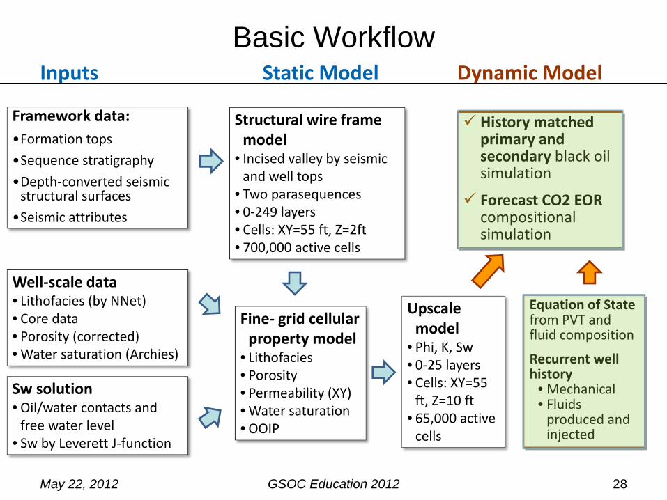
Basic Workflow

Framework data:•Formation tops

•Sequence stratigraphy

•Depth‐converted seismic structural surfaces

•Seismic attributes

Structural wire frame model

• Incised valley by seismic and well tops

• Two parasequences • 0‐249 layers• Cells: XY=55 ft, Z=2ft• 700,000 active cells

Dynamic Model

Well‐scale data• Lithofacies (by NNet)• Core data• Porosity (corrected)• Water saturation (Archies)

Fine‐ grid cellular property model

• Lithofacies• Porosity• Permeability (XY)• Water saturation• OOIP

Sw solution• Oil/water contacts and free water level

• Sw by Leverett J‐function

Inputs Static Model

Equation of Statefrom PVT and fluid composition

Recurrent well history

• Mechanical• Fluids produced and injected

History matched primary and secondary black oil simulation

Forecast CO2 EORcompositional simulation

Upscale model

• Phi, K, Sw• 0‐25 layers• Cells: XY=55 ft, Z=10 ft

• 65,000 active cells


Field Summary

Chester IV (Pleasant Prairie South) cuts through Pleasant Prairie, a faulted anticline producing from the St. Louis (34 mmbo).

Meramec structure (CI = 20 ft) and Chester IVF gross thickness (color)

Chesterian incised valley

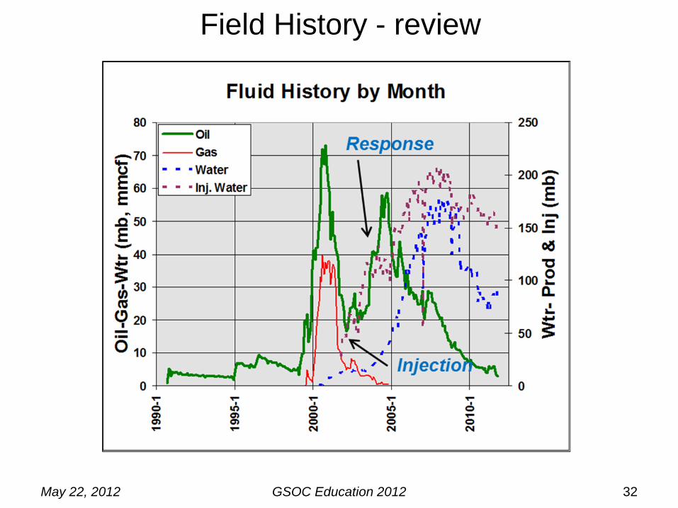
Producing zone Miss. ChesterDiscovered 1990Waterflood 2002Cumulative Oil 4.4 mmboCumulative Gas 0.7 BCF

WF recovery Appx 50% of cum.Oil wells total 18*Current oil wells 13Current wtr inj wells 9

*5 oil converted to injectors

Injection

Response


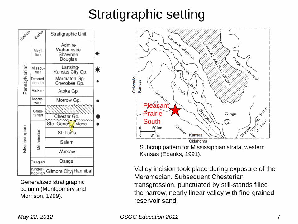
Stratigraphic setting

Generalized stratigraphic column (Montgomery and Morrison, 1999).

Valley incision took place during exposure of the Meramecian. Subsequent Chesterian transgression, punctuated by still-stands filled the narrow, nearly linear valley with fine-grained reservoir sand.

Subcrop pattern for Mississippian strata, western Kansas (Ebanks, 1991).

Pleasant Prairie South


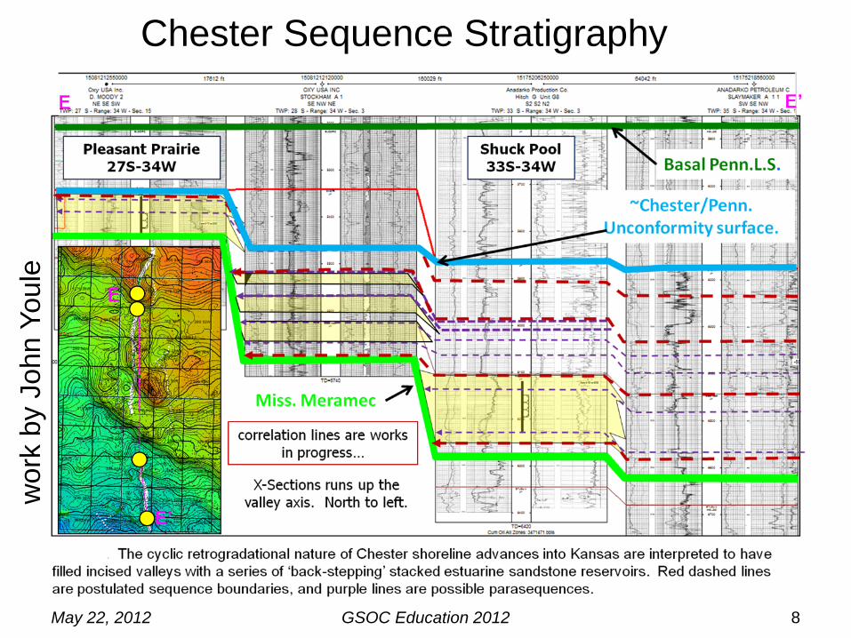
Chester Sequence Stratigraphyw

ork

by J

ohn

Youl

e


Basic Workflow








Dynamic Model






Inputs Static Model






Upscale model




Lithofacies in core and wireline logs

Two cores of nearly entire Chester IVF

• Lithofacies• Petrophysics

limey congl

wkly strat/lam ss

pebbly ss

x-bedded ss

shale

basal congl

limey congl

reservoir ss

shale

basal congl

Main LithofaciesModel Core

core wells

2.8 mi N

PS

-1P

S -2

core

d in

terv

al

core

d in

terv

al

parasequence boundary


Lithofacies in core and wireline logs

St. Louis

ChesterBasal Congl.

Pebbly Sandstone

(5124)

5218.5 (5213.5)

X-bedded Sandstone

Laminated Sandstone

Limey Congl.

(5152.5)

5148.5 (5156)

(log depth)

5240.5 (5235.5)


Define lithofacies in wells without coreQuestions to be answered1. Do lithofacies make a difference?2. Can they be defined in wells without core?3. Lumping and splitting decision process

• What can be defined?• What makes sense petrophysically?

They do make a differenceDecided to lump


Lithofacies estimated by Neural Network

Train Nnet on core lithofacies

Use modified jacknife approach in training

Could not differentiate 3 reservoir lithofacies

Very high success rate (>90%) with four lithofacies

Predictor variables:• Gamma Ray• Nphi-Dphi Xplot• Nphi-Dphi difference• Log10 ResDeep• PE• Relative position

curve


Basic Workflow








Dynamic Model






Inputs Static Model






Upscale model




3D Seismic Pleasant Prairie

Meramec Time Structure

KC “A”

MRRWMRMC

ARBK

PC

• Down to west bounding fault

• Chester IV cuts Pleasant Prairie anticline

• IV may be associated with deeper karst in Arbuckle

• Karsted Meramec surface evident in time structure Interpretation work by Dennis Hedke

incision

60ms fault


Meramec structure in time and depth

Meramec Time Structure CI = 2ms Meramec Seismic Depth Structure CI = 25 ft


More viewsMeramec seismic depth Morrow - Meramec Isochron

ms

50 45 40 35 30 25 20 15


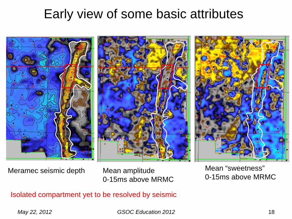
Early view of some basic attributes

Mean amplitude 0-15ms above MRMC

Mean “sweetness” 0-15ms above MRMC

Meramec seismic depth

Isolated compartment yet to be resolved by seismic


Model framework1. Build Meramec surface with 3D tied to wells2. Define PS1 and PS2 tops in 25 wells in valley and

build surfaces3. Define PS1 volume (Base IV to PS1 surface)4. Define PS2 volume (Top PS1 to PS2 surface,

bounded by IV walls) 5. Layer PS2 volume: layers follow base6. Layer PS1 volume: layers follow top7. Cell dimensions: XY=55’, Z ~2 ft

Initial modeling work by Peter Senior.

Geomod2 by Dubois.

steep walled canyon

Valley before fill

PS1 upper surface

PS2 upper surface

VE = 10


Basic Workflow








Dynamic Model






Inputs Static Model






Upscale model




Static Model Properties

Inputs: 25 valley wells with Phi, Lithofacies and SwImport LAS curves at half-foot sample rateUpscale to layer scale (2-ft)

Sandstone K(md)= 0.0047*PHI^3.9365Conglomerate K(md)= 0.0033*PHI^2.9396Shale K(md)= 0.01

Model Lithofacies• Data analysis and

variograms• Sequential indicator

simulation

Model Porosity• Data analysis and

variograms by lithofacies• Sequential Gaussian

simulation by lithofacies

Calculate Kxy by lithofacies

Estimate Sw by J-Function


Sw by Leverett J-Function1. O/W contact estimated -

2235. by operator confirmed Assume FWL~10ft below O/W contact (-2245)

2. E-Log inputs for J-Function: • PhiX - Corrected porosity

from core-log phi algorithm

• Kest - from empirically derived K-phi transform equations

• Sw_Arch – calculated Sw using standard Archies equation (m,n = 2, Rw=0.04)

3. Generate J-Function and apply at model cell scale

• Model cell inputs: Phi, K, HaFwl

• K is lithofacies sensitive, so facies is taken into account


Lithofacies and

PorosityLithofacies

Porosity(0-25%)


Water Saturation

and Permeability

Sw (0-1)

Perm xy(0.1-1000 md)


Upscale to coarse grid and export for simulation

Facies Porosity

Water Saturation Permeability

Fine-grid static model 2-ft h cells were upscaled to 10-ft h cells for simulation.

Fine-grid static model 2-ft h cells were upscaled to 10-ft h cells for simulation.


Properties at varying scalesLithofacies

Permeability XY

Porosity

Sw by J-function

shale bcgl lmy cgl sand shale bcgl lmy cgl sand

model upscaled to layer

½ foot model upscaled to layer

½ foot

fine grid coarse grid fine grid

coarse grid

fine grid

coarse grid

fine grid

coarse grid


Static Model Volumetrics

Cum. Oil Cum. Wtr Inj

twelve patterns

North

112


Basic Workflow








Dynamic Model






Inputs Static Model






Upscale model




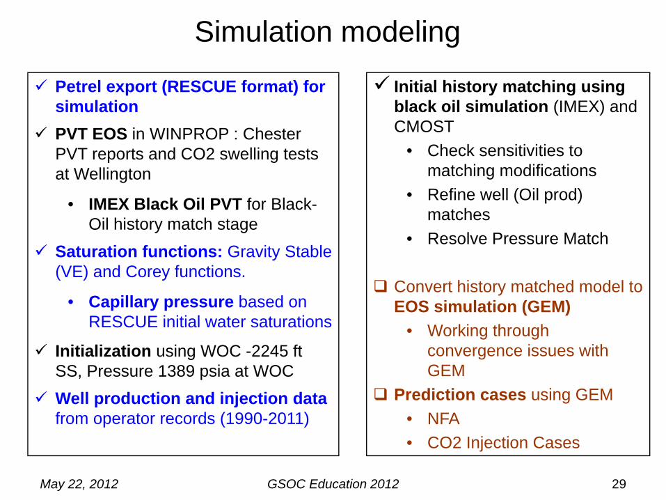
Simulation modeling

Petrel export (RESCUE format) for simulationPVT EOS in WINPROP : Chester PVT reports and CO2 swelling tests at Wellington

• IMEX Black Oil PVT for Black-Oil history match stage

Saturation functions: Gravity Stable (VE) and Corey functions.

• Capillary pressure based on RESCUE initial water saturations

Initialization using WOC -2245 ft SS, Pressure 1389 psia at WOCWell production and injection data from operator records (1990-2011)

Initial history matching using black oil simulation (IMEX) and CMOST

• Check sensitivities to matching modifications

• Refine well (Oil prod) matches

• Resolve Pressure Match

Convert history matched model to EOS simulation (GEM)

• Working through convergence issues with GEM

Prediction cases using GEM• NFA• CO2 Injection Cases


Black Oil Simulation

General workflow1. Match fluid & pressure histories (1990-2011)

2. Define 12 patterns (polygons)

3. Modify properties to attain match• Pore volume modifiers by polygon• I-Permeability modifiers by polygon • I and J Transmissibility modifiers (by polygon)• Relative permeability

• Psuedo-functions – Rocktype, VE, Stratified – by polygon• End points (SWCR, SOWR, KRW) by region

4. CMOST automation to run hundreds of iterations to

get close

5. QC and manual inputs for final

Reservoir simulation work by Eugene Williams


Simulation model views

Divided into 12 patterns for

property modification

1

7

8

12


Field History - review


Field-scale matches

Total liquids produced (bpd)

Water produced (bpd)

10000

1000

100

10

10000

1000

100

10Oil produced (bpd)

Lighter colored are actual, darker are modeled10,000

4.6 mmbo

10.7 mmbw

Water injected (bpd)

18 mmbw7,000


Example individual well matches

1000

100

10

1

10000

1000

100

10

1

10000

1000

100

10

1

1000

100

10

1

460mbo

1600mbw

670mbo

1800mbw


Discussion of modifications

Significant increase in permeability at low end• Possibility of natural fractures (some noted in core)

Reduction in mobile oil by up to 30% by polygon (by reduction in pore volume)

• Static model pore volume to high (model geometry)• Initial model Sw estimate too low• Tortuosity not modeled (barriers or baffles not accounted for)• Water bypass

Possibly several of above• Static model RF is ~31% of OOIP• Dynamic model RF is ~43% of “reduced” OOIP• RF probably somewhere in between


SummaryCharacterization, modeling and black oil simulation is fair representation of reservoir

Will proceed with CO2 EOR and storage simulation

Improvements possible

1. More seismic attribute work (could require extensive reprocessing)

2. Rebuild Petrel model for better volumetrics

3. Another complete iteration

On to the next field……complete all four in 2012


Acknowledgments

Material presented is based upon work supported by the U.S. Department of Energy (DOE) National Energy Technology Laboratory (NETL) under Grant Number DEFE0000002056. This project is managed and administered by the Kansas Geological Survey/KUCR, W. L. Watney, PI, and funded by DOE/NETL and cost-sharing partners.

Disclaimer:This report was prepared as an account of work sponsored by an agency of the United States Government. Neither the United States Government nor any agency thereof, nor any of their employees, makes any warranty, express or implied, or assumes any legal liability or responsibility for the accuracy, completeness, or usefulness of any information, apparatus, product, or process disclosed, or represents that its use would not infringe privately owned rights. Reference herein to any specific commercial product, process, or service by trade name, trademark, manufacturer, or otherwise does not necessarily constitute or imply its endorsement, recommendation, or favoring by the United States Government or any agency thereof. The views and opinions of authors expressed herein do not necessarily state or reflect those of the United States Government or any agency thereof.

We wish to thank the companies participating in the project: Anadarko Petroleum Corp.

Berexco LLC Cimarex Energy Company

Glori Oil Limited Elm III Operating, LLCMerit Energy Company

And Kansas Geological Survey, through the Kansas University Center for Research and the U.S. Department of Energy

reservoir characterization and modeling of a … characterization and modeling of a chester incised...

Documents