COVER SHEET

BMS0054: Postgraduate Research Paper (Aaron Tan)

Research Paper Journal Article: 6,000-8,000 words

Mohamed Ashour (u1573932)

By submitting this work you are confirming that you have read and understood the regulations of the University of Huddersfieldconcerning hand-in deadlines, extenuating circumstances procedures and academic misconduct. For more information see www.hud.ac.uk/regs

You are confirming that this assignment is wholly your own work unless otherwise clarified and correctly referenced as requiredby the appropriate referencing protocols.

If you do not receive an email receipt for this work within two working days, please contact your School office.Student Signature: ______________________________________________________

For office use only

u1573932 BMS005411516

Interactions of Fiscal, Monetary Policy and Output in the Advanced

Economies Before and After the Global Financial Crisis: A VAR Panel

Comparative Approach

ABSTRACT

This study investigates the interactions of fiscal policy, monetary policy and

output in the advanced economies by comparing the period before the crisis from

Q1 2000 to Q2 2008 to the period after crisis from Q3 2008 to Q4 2015. An

unrestricted VAR panel model of 3 endogenous variables is used based on

quarterly panel data of 26 advanced countries for the growth of real GDP as a

measure of output, interest rates as a measure of monetary policy and growth in

government expenses as a measure of fiscal policy. Impulse response functions

and variance decompositions are used to interpret and analyse results from the

VAR model due to the complexity of interpreting many coefficients in VAR

models which dynamically affect and depend on each other. The results imply

that the effectiveness of interest rates as a measure of monetary policy on the

growth of real GDP weakened significantly after the crisis. Moreover, variation

in monetary policy due to the growth of real GDP increased after crisis due to the

increase in utilizing interest rates to stabilize and boost the output in advanced

economies. In addition, the fiscal policy has a limited impact on output before

and after the crisis and no effect on monetary policy in both periods. Finally,

effect of output on fiscal policy weakened significantly after the crisis.

Mohamed Ahmed Ashour

12 September 2016

Thesis submitted to the University of Huddersfield

(Huddersfield University Business School)

in partial fulfilment of the requirements for the degree of

Master of Science in Economics

No portion of the work referred to in the research paper has been submitted in support of an application for another

degree of qualification of this or any other University or institute of learning

Total number of words excluding the abstract: 7997

1

1 INTRODUCTION

As achieving macroeconomic stability has become challenging in the advanced

countries after their economies were hit by the global financial crisis in 2008, it

is important to study the interactions between fiscal, monetary policy and output

in those economies and whether the effectiveness of the macroeconomic policies

is impacted compared to the period before the crisis or not.

Thus in this study, a 3 equations VAR panel model employing data from 26

advanced countries mostly from Europe and US in the period from Q1 2000 to

Q4 2015 is used to capture the dynamic interdependencies between fiscal,

monetary policy and output in the period before and after the crisis.

The study findings suggest that even though monetary policy is effective in

responding to output fluctuations before the crisis, its effectiveness weakens

significantly in the period after the crisis. Additionally, fiscal policy has a limited

effect on output before and after the crisis and no effect on monetary policy in

both periods. Nevertheless, contractionary monetary shock has a mixed effect on

fiscal policy before the crisis, i.e., government expenses increase in the short run

forecast horizon before decreasing in the longer forecast horizon, while after the

crisis the same effect is negative in the short run before being neutral in the long

run.

The rest of the study is organized as following: Section 2 reviews the literature

of coordination between fiscal and monetary policy in addition to debates

attributed to the fiscal and monetary policy before and after the crisis. Data

description is presented is section 3 followed by the econometric methodology in

section 4. Section 5 highlights the empirical analysis and interpretation of results.

Finally, the last section is for main conclusions.

2

2 LITERATURE REVIEW

2.1 Coordination between fiscal and monetary policy

The coordination between fiscal and monetary policy and the effectiveness of

both policies have been discussed extensively in the literature whether

theoretically or empirically. This section highlights a sample of this huge

published research with a special focus on how the conduct of both the fiscal and

the monetary policies might change with the occurrence of crises and

consequently affect the overall economy.

One of the pioneering studies in the area of fiscal and monetary policy

coordination is Friedman (1948) that proposes a framework involving both

policies. This framework suggests reforming the monetary system through

limiting discretion attributed to controlling money supply by the central bank. On

the other hand, the fiscal framework suggested is attributed to three aspects: the

government expenditure, social security benefits and the tax system. A common

trait among those fiscal aspects that Friedman (1948) stresses in his framework

is again related to supporting working within rules or targets rather than

discretionary actions that respond to cyclical fluctuations in the economy. This

provides a stable fiscal and monetary framework amid short run cyclical

fluctuations and avoids to a great extent uncertainty resulting from discretionary

responses (Friedman, 1948).

On the other hand, Alesina and Tabellini (1987) present an opposing view to

Friedman (1948) regarding rules vs. discretion. They show using a game

theoretic model that when monetary policy follows rules it produces a lower level

of output and public spending when coordination with fiscal policy is absent

compared to a scheme where the monetary regime follows discretion. Moreover,

Alesina and Tabellini (1987) highlight how the degree of coordination between

fiscal and monetary authorities under a discretionary regime leads to different

3

results attributed to output, government spending and taxes depending on the

level of independence of the central bank.

In their paper, Sargent and Wallace (1981) present two different scenarios for the

interaction between monetary and fiscal policy within a game theory scheme.

One in which the monetary policy is in the lead, while the other in which there is

a kind of fiscal dominance, where the monetary policy acts in response to the

fiscal policy. In the first scenario, the monetary authority sets the monetary

targets first. This results in fiscal policy being constrained by those targets when

planning the budget and setting the fiscal targets. Consequently, under this

scenario inflation is well controlled by the monetary policy, while in the second

scenario Sargent and Wallace (1981) propose another model where there is a kind

of fiscal dominance, in which the fiscal authority sets the budget and announces

all related fiscal targets. As a result, the monetary authority follows the fiscal

authority and is limited by the fiscal targets that should be achieved. This results

in higher inflation due to the increase in money supply created to meet the fiscal

needs.

Blinder (1982) builds on the idea of the two scenarios that Sargent and Wallace

(1981) presented and discusses which of the two policies or authorities should

have the higher hand. Blinder (1982) elaborates that it is challenging to decide

which authority is always right or superior over the other, therefore it is better to

balance the power between both authorities so that no authority is dominant over

the other. Moreover, Blinder (1982) illustrates why coordination might be weak

or absent between both policies which is due to the lack of a common objective

between the two policies or authorities. Under these conditions of uncertainty on

whether fiscal or monetary policy should be in control and the lack of common

objectives non-coordination between both policies might be the best option

(Blinder, 1982).

Another paper that tackles important issues and challenges related to

coordination between monetary and fiscal policies is Laurens and De La Piedra

4

(1998) which discusses policy coordination in the short and long run, the

consequences of lack of policy coordination, the importance of timing in

coordination, and how coordination differs under fixed vs. flexible exchange rate

regimes. Regarding policy coordination in the short and the long run, Laurens

and De La Piedra (1998) mention that priority should be given to the monetary

policy to achieve price stability, as well as management of the public debt.

Nevertheless, the next stage after attaining price stability is attributed to

achieving sustainable growth and controlling inflation. This takes place through

coordination between both policies, in the long run, to guarantee that any fiscal

deficits stay within the level, where they can be financed through capital markets

without resorting to external borrowing or increasing the money supply by the

central bank as it will result in inflationary pressures.

Weak or lack of coordination can lead to different scenarios similar to those

presented earlier by Sargent and Wallace (1981). First is a scenario in which the

monetary policy presented by the central bank determines its monetary targets

without accommodating the financing needs of the government. As a result, the

government would be restricted by the domestic and foreign borrowing available.

A second scenario that Laurens and De La Piedra (1998) mention is a scheme of

fiscal dominance where the fiscal authority presented by the ministry of finance

determines the fiscal needs solely which enforce the monetary authority to

finance those deficits through monetary base expansion which increases

inflationary pressures, in addition to pressures attributed to maintaining exchange

rate in fixed exchange rate regimes which result in distortion in the levels of

international reserves.

An important point which Laurens and De La Piedra (1998) state is related to

how both the monetary and fiscal policies function differently when it comes to

time. The same view is also shared by Arestis and Sawyer (2004a) who point out

that monetary policy is implemented in a quicker manner that is more flexible to

adjustments on a daily basis compared to fiscal policy which cannot be adjusted

5

as quickly and smoothly as the monetary policy due to political aspects related

to getting approvals through parliament for any government expenditures leading

to policy lags. In addition to other challenges such as the ‘ratchet effect’ which

is usually associated with the fiscal policy specifically when increasing

government expenditures is needed, but politically infeasible (Arestis and

Sawyer, 2004a).

Laurens and De La Piedra (1998) show that the room given to each policy differs

based on the exchange rate system, where in a fixed exchange rate regime the

role of the monetary policy is limited as it becomes mainly a follower to the

monetary policy of the economy to which the local currency is pegged to.

Therefore, most of the burden falls on the fiscal policy to stabilize the economy.

The opposite is completely true in a flexible exchange rate regime, where the

monetary policy has more space to operate and as a result is more effective.

Eggertsson (2006) elaborates that the coordination between fiscal and monetary

policy is preferable when the economy is witnessing deflationary pressures. This

coordination between both policies leads to maximizing social welfare that is

reflected in figures of fiscal multipliers for real and deficit spending which are

found to be higher under a coordinated policy compared to an uncoordinated one.

On the other hand, Eggertsson (2006) states that an uncoordinated scheme results

in the central bank operating independently to achieve inflation and output targets

without taking into consideration the implications on fiscal policy.

Niemann and Hagen (2008) agree with Laurens and De La Piedra (1998) that the

monetary policy is more effective compared to fiscal policy in stabilizing short-

run fluctuations in the economy. Besides, Niemann and Hagen (2008) elaborate

how fiscal policy can pressure the monetary policy and affect how it operates by

highlighting the concept of fiscal space presented also by Mates (2011), who

shows how the fiscal space size affected the room the fiscal policy had to function

during the global financial crisis. Moreover, Niemann and Hagen (2008)

demonstrate how both policies are interrelated especially in the long run.

6

Hutchison, Noy and Wang (2010) study 83 different crises in 66 countries by

setting a model that explains how output growth is affected by crises besides the

effect of fiscal and monetary policy. Hutchison et al. (2010) conclude that

contractionary fiscal and monetary policy during crises intensifies slowdowns

and may strongly lead to large output losses. Additionally, they find that

discretionary fiscal expansion does not lead to large output losses as usually

shown in the literature, while expansionary monetary policy has no clear effect.

Additionally, Li (2013) studies how effective fiscal and monetary policies are

during several crises from 1977 to 2010. Li (2013) finds that while expansionary

fiscal policy does not have any influence in shortening crises, a mild

expansionary monetary policy is influential in shortening the duration of crises

compared to an aggressive expansionary monetary policy which is impotent. On

the other hand, Li (2013) observes that contractionary monetary policy

exacerbates crises.

Arestis (2015) supports giving a wider room for fiscal policy, as he argues that it

is effective in increasing employment rates through its effect on aggregate

demand which could be boosted if coordinated with monetary policy.

2.2 Evolution of fiscal and monetary policy debates

This subsection reviews how ideas related to fiscal and monetary policy have

evolved recently, and how debates around both policies have intensified and

increased resulting in reviewing and reconsidering the conventional framework

specifically after the global financial crisis.

Arestis and Sawyer (2004a) and Arestis and Sawyer (2004b) highlight how in the

years before the global financial crisis the monetary policy had the upper hand

compared to the fiscal policy — a phenomenon which changed after the crisis

with the fiscal policy restoring some of its lost influence.

7

Some reasons behind this domination of the monetary vs fiscal policy as shown

by Arestis and Sawyer (2004b) are first the abandonment of targeting

unemployment as the main goal of the macroeconomic policy in favour of

inflation. Additionally, restricting the usage of fiscal policy to be used only as an

automatic stabilizer within a constrained budget, as well as the downgrade of the

fiscal policy in favor of the monetary policy in boosting the economy and dealing

with fluctuations since monetary policy is quicker in implementation compared

to fiscal policy.

2.2.1 Monetary Policy debates

Arestis and Sawyer (2004a) mention that the monetary policy developed from

trying to control the money supply to trying to target and control inflation through

interest rates as its main goal starting from the second half of the 1980s. This

approach continued until the occurrence of the global financial crisis which led

to some demands to widen the scope of the monetary policy, as suggested by

Arestis and Sawyer (2012), who contend that the main objective of monetary

policy and central banks should be the financial stability, not targeting of

inflation. This resulted from the attention given to financial regulation and

supervision after the disorder caused by shadow banking and financial

engineering during the crisis.

Blanchard (2012), Blanchard (2011a) and Blanchard, Dell’Ariccia and Mauro

(2013) reinforce the argument of Arestis and Sawyer (2012) that the crisis has

revealed that inflation and output should not only be the targets of monetary

policy and that policy rate is not the only instrument needed to maintain

macroeconomic stability. Moreover, according to Blanchard (2011b), the crisis

has shown how stable inflation and output which is near potential can distract

policymakers and economists from risky hidden imbalances such as those related

to highly leveraged financial institutions, high private debt, excess maturity

8

mismatches, etc., all of which have led to shedding more light on the importance

of using macro-prudential tools in order to monitor those imbalances and achieve

financial stability beside achieving macroeconomic stability through monetary

policy by using the policy rate as pre-crisis. (Blanchard et al., 2013; Blanchard,

2012; Blanchard, 2011a).

Stiglitz (2012) points out that one of the main the reasons that led to the crisis is

the dependence of economists on economic models that are not inclusive, which

affected the monetary policy decisions. Stiglitz (2012) elaborates this by

explaining how credit is used as equivalent to money in these times which is

acceptable in normal times since both variables are highly correlated. However,

during crises, this relationship is not valid or accurate. Another point that has to

be taken into consideration is the importance of coordination between different

instruments to achieve different objectives in policy-making, as the crisis

revealed how the absence of coordination can be inefficient to the final outcome

of the policy (Stiglitz, 2012).

A controversial topic that caught a lot of attention in academia after the crisis is

attributed to the monetary stimulus that a lot of countries worldwide undertook

after the crisis to stimulate their economies. The controversy arises from the

effectiveness of the stimulus and whether it is beneficial to put the economy back

on the right track or not. Mishkin (2009) argues that monetary policy is effective

during financial crises, and disagrees with those who claim that easing monetary

policy is ineffective. Mishkin (2009) claims that following a tight monetary

policy during the crisis would have made the slowdown worse as consumer

spending and investments would have been more constrained creating more

uncertainty and risk which would have been reflected in higher interest rates of

treasury securities.

Bouis et al. (2013) disagree with Mishkin (2009), arguing that monetary stimulus

can affect the recovery of the economy negatively as a result of rolling over risky

9

debt smoothly with the help of low interest rates which they state was observed

by different studies in some countries in the OECD.

To sum up, it is important to understand that the crisis revealed that the financial

sector and the economy are interrelated where any disruption in the financial

sector is reflected in the economy and vice versa. Therefore, macro-prudential

tools are needed in order to achieve financial stability which cannot be achieved

only by targeting inflation and output stability. Moreover, the crisis exposed the

dilemma of the zero lower bound which was earlier thought to be a phenomenon

that does not persist for a long time. However, after the crisis, the opposite was

proved which exposed the limits of conventional policy specifically in

responding to further shocks and prolonged slowdown. Lastly, though aggressive

monetary stimuli were implemented, it is important to understand that recovery

after recessions resulting from crises is not as rapid as after normal recessions —

in other words, V-shaped recoveries do not occur (Mishkin, 2011; Reinhart and

Reinhart, 2010).

2.2.2 Fiscal Policy debates

Moving to the evolution of the fiscal policy and how the global financial crisis

affected it, Blanchard, Dell’Ariccia and Mauro (2010) state that fiscal policy has

been inferior to monetary policy in the two decades ahead of the crisis, a view

which is supported by many others such as Arestis and Sawyer (2004a). This

retreat was due to many reasons according to Blanchard et al. (2010). The first

being the controversy surrounding the effectiveness of fiscal policy to stimulate

the economy due to the Ricardian equivalence. Additionally, the success of

monetary policy in stabilizing the output before the crisis during what economists

call the Great Moderation. Furthermore, the speed associated with the

implementation of monetary policy compared to fiscal policy which is hindered

by parliamentary decisions leading to lags which make the fiscal policy not as

10

suitable for short term fluctuations or slowdowns as the monetary policy.

Consequently, the usage of fiscal policy as a countercyclical tool ahead of the

crisis was most of the time limited to the automatic stabilizers, especially in

advanced economies which had the upper hand compared to the discretionary

fiscal measures (Blanchard et al., 2010).

According to Blanchard et al. (2010), the crisis was the main trigger behind

pulling back the fiscal policy from being inferior to the monetary policy to being

more or less equivalent in importance. This was due to the mainstream realization

that the monetary policy with all its conventional and unconventional instruments

had nothing more to offer, especially as time showed that the recession was not

going to be short, and therefore resorting to fiscal stimulus was inevitable.

Mates (2011) shows how fiscal policy has risen back to the main stage during the

crisis. The reaction towards fiscal policy has developed as the crisis passed

through different stages and events kept unfolding. Fiscal policy was limited at

the beginning to the implementation of the automatic stabilizers due to the fears

of increasing expenditures and indebtedness that could lead to fiscal deterioration

as a result of any discretionary fiscal measures (Mates, 2011).

Things started to change with the crisis starting to be felt on a larger scale after

the collapse of Lehman Brothers in 2008 and with discretionary fiscal stimuli

getting approvals in most of the advanced economies. However, pressures on

fiscal spaces started to accumulate in some countries like Greece which led again

to the controversy around fiscal discretionary relaxation and how it pressures

fiscal spaces especially in countries that face challenges attributed to their current

account and budget deficit figures (Mates, 2011).

Mates (2011) notes that the effect of automatic stabilizers together with monetary

stimuli was more substantial than that of discretionary stimuli, which contributed

to imbalances as well as debt problems in countries that do not have enough fiscal

space.

11

Indrawati (2012) states that introducing automatic stabilizers even if it is just

limited to a certain period of time is important for quicker fiscal effect. Moreover,

Indrawati (2012) highlights the importance of expenditure that generates

employment as well as capital expenditure which creates jobs and leads to output

growth.

An important challenge that rises with the crisis is attributed to fiscal

consolidation and its speed. Some strategies for fiscal consolidation include

expanding the tax base to increase tax revenues as an automatic stabilizer, besides

limiting discretionary spending and improving the quality of spending

(Indrawati, 2012).

Nevertheless, it is important to take into consideration that fiscal consolidation

can increase income inequality which is simply due to the decrease in output and

employment in the short run, which is reflected in lower consumption and

incomes (Arestis, 2015).

Finally, we can conclude that the crisis has shed light on the following fiscal

policy lessons. First, fiscal space is very important when it comes to using fiscal

stimuli in absorbing economic shocks: the larger the fiscal space the more fiscal

stimuli can be used to stimulate the economy and vice versa. Furthermore, the

crisis showed that fiscal policy can be used to stabilize the economy in the short

run when the monetary policy reaches its limits, as the crisis reinforced strongly

the evidence of fiscal policy effectiveness (Romer, 2012).

3 DATA

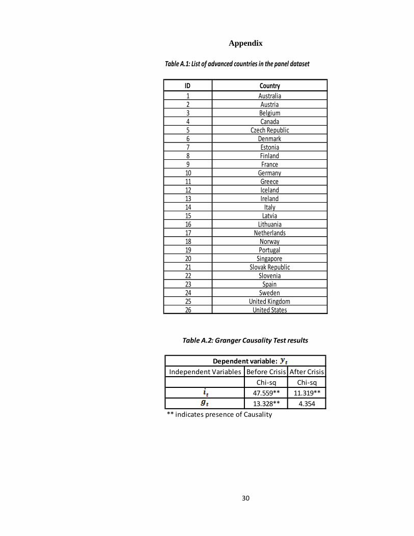
The dataset used in this study is a panel dataset which consists of 26 countries of

the advanced economies1 most of which are from Europe in addition to the United

States as per the classification of the World Economic Outlook database of the

1 List of the countries included are in Table A.1 in the Appendix

12

IMF. The focus on Europe and the United States in the dataset is due to the fact

that both represent the majority of the advanced economies that were affected by

the global financial crisis. The period of the study is from Q1 2000 to Q4 2015

consisting of 1664 observations divided into 2 parts to examine how the

interaction of fiscal policy, monetary policy and output differed before and after

the crisis in the advanced economies. Part 1 consists of 884 observations from

Q1 2000 to Q2 2008 representing the period before the crisis. Part 2 is from Q3

2008, which coincides with the collapse of Lehman Brothers in the US and is

considered the triggering event that led to the spread of the crisis worldwide, to

Q4 2015 representing the period after the crisis. The variables used in this study

are 𝒚𝒕 , 𝒊𝒕 and 𝒈𝒕. 𝒚𝒕 is a proxy for output which represents the year on year

(YoY) growth rate of real GDP on quarterly basis. The data for this variable is

extracted in this form from the International Financial Statistics Database (IFS)

of the IMF. The reason behind using YoY growth of GDP and not the absolute

value is to avoid the seasonality of numbers and to overcome the problem of GDP

figures reported in national currencies. 𝒊𝒕 is a proxy for monetary policy which

represents the official interest rate announced by the central bank in each country

on a quarterly basis. The data for this variable is extracted from the IFS database.

There are some challenges that were faced while extracting interest rate data —

firstly, although the central bank (CB) policy rate is the official rate for most of

the countries in the dataset of the study, for some countries it is not. Therefore,

the IFS notes were checked for countries to figure out what is the official interest

rate announced by central banks in those countries. It was found that in some

countries the official interest rate is the discount rate, for others it is the money

market rate and for some countries the official rate is the repo rate. Moreover, the

majority of the countries in the dataset are in the Euro Area, consequently the

central bank policy rate of the ECB is used for those countries starting from the

date of joining the Euro Area, which for most of the countries in the dataset is

before Q1 2000. However, for countries that joined after Q1 2000 or recently, the

official rate of their central banks is followed whether it is the discount rate or

13

the CB policy rate or the money market rate, etc. till the date of joining Euro Area

after which the CB policy rate announced by the ECB was followed as in the rest

of countries in the Euro Area. 𝒈𝒕 is a proxy for fiscal policy which represents the

YoY growth rate of government expenses of each country on a quarterly basis.

General government expenses quarterly figures are extracted from the IFS

database in absolute figures then YoY growth rates for the quarterly figures were

calculated in order to overcome the fact that the data is available only in national

currencies. Additionally, this avoids seasonality of data that could occur if the

growth rate for quarterly government expenses is calculated on Quarter on

Quarter (QoQ) basis and not YoY basis. The choice of the 3 variables 𝒚𝒕 , 𝒊𝒕 and

𝒈𝒕 is based on the related literature specifically on Senbet (2011) and Mitreska

et al. (2010).

4 ECONOMETRIC METHODOLOGY

4.1 Background on VAR models

The main goal of this paper is to study how fiscal and monetary policy interacted

before and after the crisis in the advanced economies, and how this interaction

affects the output in these economies. This paper uses the vector autoregression

(VAR) model which has become commonly used in macroeconomic time series

modelling after Sims (1980) highlighted it as a technique that can be applied to

elaborate dynamic relationships and interdependencies among a group of

variables. The triggering point that contributed to the development of VAR

models to be used in macroeconomic modelling is attributed to the fact that

traditional simultaneous equation models that were used previously before Sims

(1980) introduced VAR models are associated with the problem of identification.

This is usually solved by enforcing some restrictions that according to Sims

(1980) have no solid justifications. As a result, an unrestricted VAR model was

developed by Sims (1980) in which all variables are treated equally without any

14

differentiation between endogenous and exogenous variables as in the restricted

conventional simultaneous equations model. In addition, the number of variables

should be equal in all equations within the VAR model (Gujarati, 2015).

A reduced mathematical form of the VAR panel model followed in this paper is

as following:

𝒚𝒕 = 𝜷𝟏 𝒚𝒕−𝟏 + 𝜷𝟐𝒚𝒕−𝟐 + ….+ 𝜷𝒑 𝒚𝒕−𝒑 + 𝜺𝒕

Where 𝑦𝑡 is a (k × 1) vector of endogenous variables, k is the number of

endogenous variables, 𝛽1 , 𝛽2 , …., 𝛽𝑝 are (k × k) matrices of coefficients to be

estimated, and 𝜖𝑡 is a (k × 1) vector of error terms, which is also called the shocks

or impulses. According to Canova and Ciccarelli (2013), the only difference

between VAR models and VAR panel models is the inclusion of a cross sectional

dimension in the VAR panel models.

4.2 VAR methodology and Fiscal and Monetary policy interaction

VAR models have been extensively used to study the interaction between fiscal

and monetary policies, their effectiveness and how they affect output. Coric,

Simovic and Deskar-Skrbic (2015) analyse the interaction of fiscal and monetary

policy in Croatia from 2004 to 2012 using a VAR model and find that both

expansionary fiscal and monetary policy contributed positively to the economic

growth in Croatia. Furthermore, Coric et al. (2015) demonstrate that the

coordination between both policies can help maintain price stability, in addition

to achieving economic growth.

Semmler and Zhang (2004) study the interaction of fiscal and monetary policy in

the Economic and Monetary Union of the EU (EMU), specifically in Italy,

Germany and France between 1979 and 1998 using a VAR model. Not only did

Semmler and Zhang (2004) find that there was a weak interaction between the

15

common EMU monetary policy and the individual fiscal policies of member

countries, but also both policies were found to be counteractive to each other.

Senbet (2011) examines how the fiscal policy presented by government expenses

and monetary policy presented by federal funds rate and non-borrowed reserves

affected the output in the USA between 1959 and 2010 using a VAR model.

Additionally, Senbet (2011) finds that monetary policy is more effective on

output compared to fiscal policy which did not have a solid impact on the output

in the USA.

Muscatelli, Tirelli and Trecroci (2002) use the VAR models to analyse how fiscal

and monetary policy in some countries of the G7 group respond to the

macroeconomic targets. They find that both policies acted as complements to

each other, meaning that when the policy is expansionary the other policy follows

the same route and vice versa. However, Muscatelli et al. (2002) find that fiscal

policy reaction to the business cycles has weakened since the 1980s.

Moreover, Petrevski, Bogoev and Tevdovski (2016) estimate a VAR model to

examine how the interaction between fiscal and monetary policy affect the South-

Eastern European Economies in the period from 1999 to 2011. Petrevski et al.

(2016) find that contractionary fiscal measures lead to an increase in economic

activity which contradicts with Coric et al. (2015) findings in Croatia. In addition,

Petrevski et al. (2016) point out that the monetary policy reaction to output and

inflation is not unexpected, i.e., monetary tightening has led to the decline of both

inflation and output. As well they highlight the fact that in the South-Eastern

European Economies under study both policies have been substitutes to each

other, i.e., monetary tightening is associated with fiscal expansion and vice versa.

4.3 Advantages of VAR methodology

The popularity that the VAR methodology has gained within macroeconomic

modelling to capture the interdependencies among different variables,

16

specifically those dynamic relationships between fiscal policy, monetary policy

and output is due to several qualities in VAR models. First, compared to the

conventional simultaneous equations method, the VAR is method is simpler and

all variables are usually treated equally, i.e., all variables are usually endogenous

(Gujarati, 2016). In just a few cases, exogenous variables are added to highlight

different seasons or a different point in time (Gujarati, 2016). Another point that

makes VAR models common in the literature of fiscal and monetary policy

interaction is the simplicity of estimating them, as the OLS method can be used

to estimate each equation in the model on a single basis, in addition to the more

efficient forecasts VAR models can provide compared to the simultaneous

equation models (Gujarati, 2016).

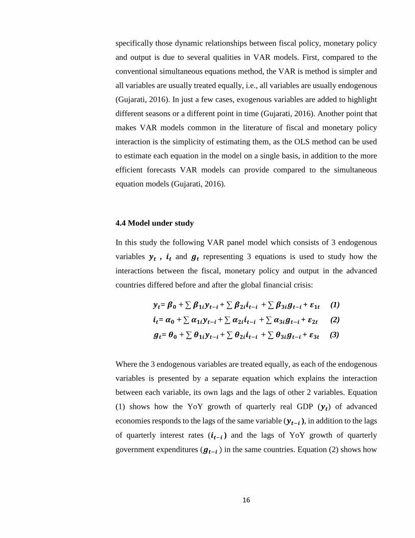
4.4 Model under study

In this study the following VAR panel model which consists of 3 endogenous

variables 𝒚𝒕 , 𝒊𝒕 and 𝒈𝒕 representing 3 equations is used to study how the

interactions between the fiscal, monetary policy and output in the advanced

countries differed before and after the global financial crisis:

𝒚𝒕= 𝜷𝟎 + ∑ 𝜷𝟏𝒊𝒚𝒕−𝒊 + ∑ 𝜷𝟐𝒊𝒊𝒕−𝒊 + ∑ 𝜷𝟑𝒊𝒈𝒕−𝒊 + 𝜺𝟏𝒕 (1)

𝒊𝒕= 𝜶𝟎 + ∑ 𝜶𝟏𝒊𝒚𝒕−𝒊 + ∑ 𝜶𝟐𝒊𝒊𝒕−𝒊 + ∑ 𝜶𝟑𝒊𝒈𝒕−𝒊 + 𝜺𝟐𝒕 (2)

𝒈𝒕= 𝜽𝟎 + ∑ 𝜽𝟏𝒊𝒚𝒕−𝒊 + ∑ 𝜽𝟐𝒊𝒊𝒕−𝒊 + ∑ 𝜽𝟑𝒊𝒈𝒕−𝒊 + 𝜺𝟑𝒕 (3)

Where the 3 endogenous variables are treated equally, as each of the endogenous

variables is presented by a separate equation which explains the interaction

between each variable, its own lags and the lags of other 2 variables. Equation

(1) shows how the YoY growth of quarterly real GDP (𝒚𝒕) of advanced

economies responds to the lags of the same variable (𝒚𝒕−𝒊 ), in addition to the lags

of quarterly interest rates (𝒊𝒕−𝒊 ) and the lags of YoY growth of quarterly

government expenditures (𝒈𝒕−𝒊 ) in the same countries. Equation (2) shows how

17

the quarterly interest rates in the advanced economies (𝒊𝒕 ) respond to its lags

(𝒊𝒕−𝒊 ) and the lags of YoY growth of quarterly real GDP (𝒚𝒕−𝒊 ), in addition to

the lags of YoY growth of quarterly government expenditures (𝒈𝒕−𝒊 ) in the same

countries. Equation (3) shows how the YoY growth of quarterly government

expenditures (𝒈𝒕 ) in the advanced economies respond to its lags (𝒈𝒕−𝒊 ), as well

as the lags of YoY growth of quarterly real GDP (𝒚𝒕−𝒊 ) and the lags of the lags

of quarterly interest rates (𝒊𝒕−𝒊 ).

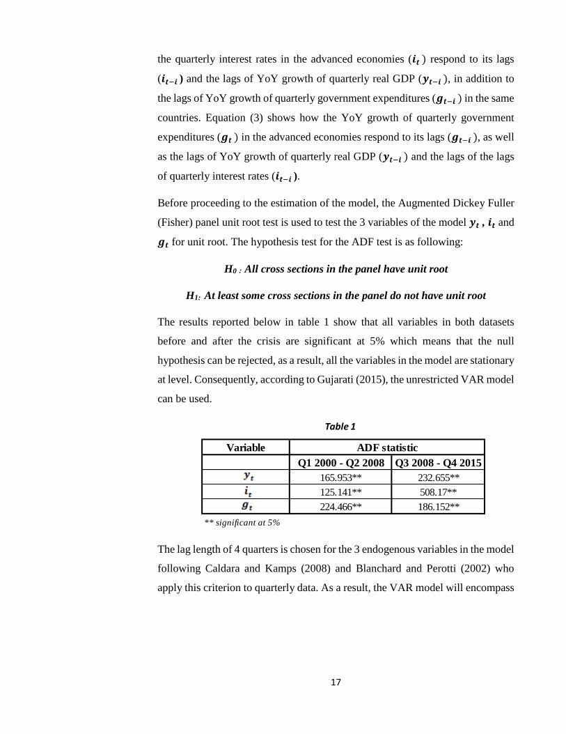
Before proceeding to the estimation of the model, the Augmented Dickey Fuller

(Fisher) panel unit root test is used to test the 3 variables of the model 𝒚𝒕 , 𝒊𝒕 and

𝒈𝒕 for unit root. The hypothesis test for the ADF test is as following:

H0 : All cross sections in the panel have unit root

H1: At least some cross sections in the panel do not have unit root

The results reported below in table 1 show that all variables in both datasets

before and after the crisis are significant at 5% which means that the null

hypothesis can be rejected, as a result, all the variables in the model are stationary

at level. Consequently, according to Gujarati (2015), the unrestricted VAR model

can be used.

The lag length of 4 quarters is chosen for the 3 endogenous variables in the model

following Caldara and Kamps (2008) and Blanchard and Perotti (2002) who

apply this criterion to quarterly data. As a result, the VAR model will encompass

Table 1

Variable

Q1 2000 - Q2 2008 Q3 2008 - Q4 2015

165.953** 232.655**

125.141** 508.17**

224.466** 186.152**

** significant at 5%

ADF statistic

18

78 coefficients out of which 72 are attributed to the lags of the 3 endogenous

variables and the remaining 6 are intercepts before and after the crisis.

5 EMPIRICAL RESULTS

5.1 Results of coefficients

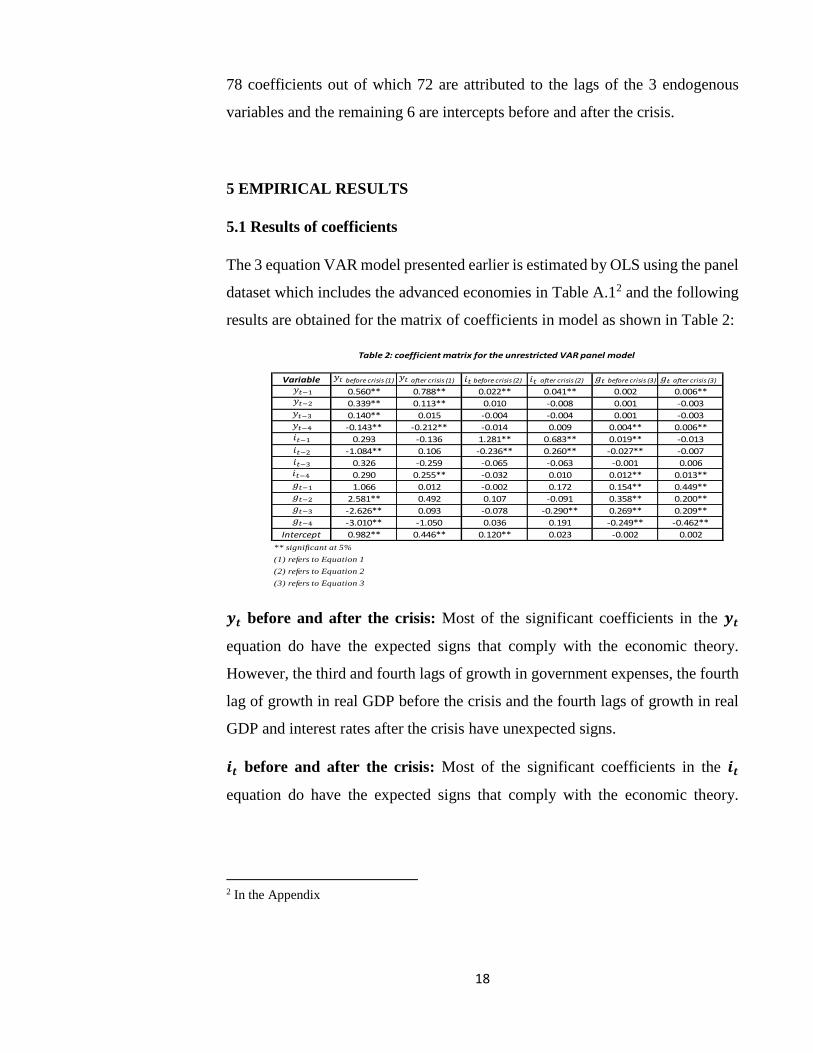
The 3 equation VAR model presented earlier is estimated by OLS using the panel

dataset which includes the advanced economies in Table A.12 and the following

results are obtained for the matrix of coefficients in model as shown in Table 2:

𝒚𝒕 before and after the crisis: Most of the significant coefficients in the 𝒚𝒕

equation do have the expected signs that comply with the economic theory.

However, the third and fourth lags of growth in government expenses, the fourth

lag of growth in real GDP before the crisis and the fourth lags of growth in real

GDP and interest rates after the crisis have unexpected signs.

𝒊𝒕 before and after the crisis: Most of the significant coefficients in the 𝒊𝒕

equation do have the expected signs that comply with the economic theory.

2 In the Appendix

Variable before crisis (1) after crisis (1) before crisis (2) after crisis (2) before crisis (3) after crisis (3)

0.560** 0.788** 0.022** 0.041** 0.002 0.006**

0.339** 0.113** 0.010 -0.008 0.001 -0.003

0.140** 0.015 -0.004 -0.004 0.001 -0.003

-0.143** -0.212** -0.014 0.009 0.004** 0.006**

0.293 -0.136 1.281** 0.683** 0.019** -0.013

-1.084** 0.106 -0.236** 0.260** -0.027** -0.007

0.326 -0.259 -0.065 -0.063 -0.001 0.006

0.290 0.255** -0.032 0.010 0.012** 0.013**

1.066 0.012 -0.002 0.172 0.154** 0.449**

2.581** 0.492 0.107 -0.091 0.358** 0.200**

-2.626** 0.093 -0.078 -0.290** 0.269** 0.209**

-3.010** -1.050 0.036 0.191 -0.249** -0.462**

Intercept 0.982** 0.446** 0.120** 0.023 -0.002 0.002

** significant at 5%

(1) refers to Equation 1

(2) refers to Equation 2

(3) refers to Equation 3

Table 2: coefficient matrix for the unrestricted VAR panel model

𝑦𝑡−1𝑦𝑡−2𝑦𝑡− 𝑦𝑡− 𝑡−1 𝑡−2

𝑡−

𝑡 𝑡𝑦𝑡𝑦𝑡 𝑡 𝑡

𝑡−

𝑡−1 𝑡−2 𝑡− 𝑡−

19

However, the second lag of interest before the crisis and the third lag of growth

in government expenses after the crisis have unexpected signs.

𝒈𝒕 before and after the crisis: Most of the significant coefficients in the 𝒈𝒕

equation do have the expected signs that comply with the economic theory.

However, the fourth lag of growth in government expenses before and after the

crisis have unexpected signs.

5.2 Results of impulse response functions and variance decompositions

As there are a lot of coefficients in VAR panel models — 78 coefficients in the

model of this study. Therefore, a better approach — to interpreting the data and

analysing in this case how the interactions between fiscal, monetary policy and

output have changed before and after the crisis — is using impulse response

functions (IRFs) and variance decompositions.

5.2.1 Interpretations of IRFs

The IRF captures how the dependent variables 𝒚𝒕 , 𝒊𝒕 and 𝒈𝒕 respond to shocks

in the error terms 𝜺𝟏𝒕, 𝜺𝟐𝒕, 𝜺𝟑𝒕 in equations (1), (2) and (3). A change in the error

terms will change current values of y, i and g, in addition to their future values

since the lagged variables of y, i and g appears in the 3 equations of the model.

A simple Mathematical formula for IRF is as following:

IRF = 𝛿𝑦𝑎,𝑡

𝛿 𝑏,𝑡−1

Which shows how variable a responds to a shock in variable b from time t to

time t-1.

20

Figures 1 and 2 show the IRFs for the model before and after the crisis. As shown

in Figures 1 and 2, while growth in real GDP before the crisis responds negatively

to the contractionary shock of monetary policy (increase in interest rates) from

the second quarter onwards. The response to the same effect after the crisis is not

as strong as before the crisis, which implies that monetary policy represented by

interest rates has become less effective — which is expected, given that interest

rates have hit their zero lower bound in most of the advanced economies in the

period after the crisis.

The response of growth in real GDP to an expansionary shock of fiscal policy

(increase in growth of government expenses) is nearly the same before and after

the crisis, where growth in GDP increases from the second quarter to the third

quarter before levelling off until the sixth quarter before starting to decline.

The response of monetary policy represented by interest rates to a shock in real

GDP growth is countercyclical before and after crisis as shown in Figures 1 and

2.

An expansionary shock of fiscal policy (increase in growth of government

expenses) has almost no effect on monetary policy before and after the crisis, i.e.,

no effect on interest rates, which is consistent with the results of Granger

causality presented in Table A.3.3

A shock to growth in real GDP leads to an expansionary fiscal policy (increase

in growth of government expenses) before the crisis, however, the response to

the same effect is weak after the crisis, i.e., nearly no significant effect as shown

in Figures 1 and 2.

Before the crisis, a contractionary shock of monetary policy (increase in interest

rates) leads to a short-term increase in growth of government expenses before it

drops from the third quarter, while after the crisis the response to the same effect

3 In the Appendix

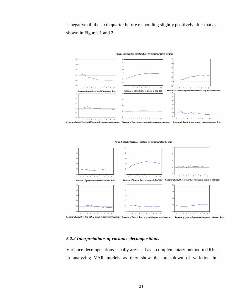
21

is negative till the sixth quarter before responding slightly positively after that as

shown in Figures 1 and 2.

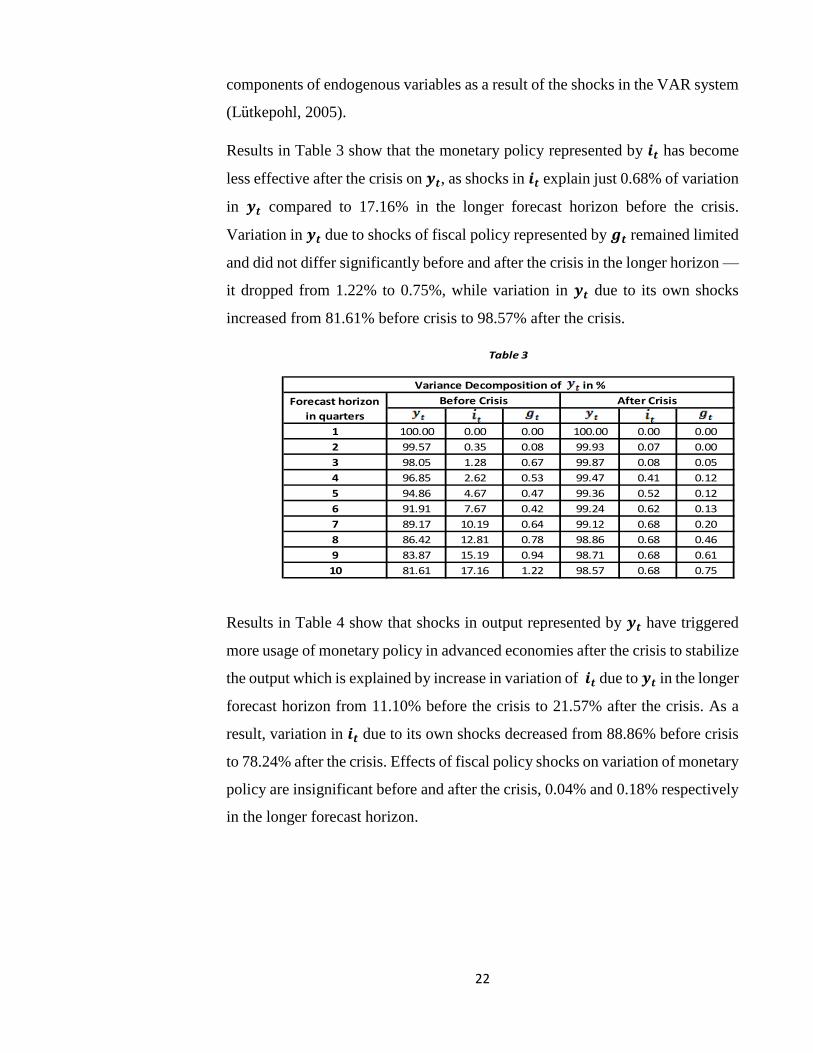
5.2.2 Interpretations of variance decompositions

Variance decompositions usually are used as a complementary method to IRFs

in analyzing VAR models as they show the breakdown of variation in

-1.0

-0.5

0.0

0.5

1.0

1.5

1 2 3 4 5 6 7 8 9 10

Response of growth in Real GDP to Interest Rates

-1.0

-0.5

0.0

0.5

1.0

1.5

1 2 3 4 5 6 7 8 9 10

Response of growth in Real GDP to growth in government expenses

-.2

-.1

.0

.1

.2

.3

.4

.5

.6

1 2 3 4 5 6 7 8 9 10

Response of Interest rates to growth in Real GDP

-.2

.0

.2

.4

.6

1 2 3 4 5 6 7 8 9 10

Response of Interest rates to growth in government expenses

Response of Growth in government expenses to growth in Real GDP

-.01

.00

.01

.02

.03

.04

.05

1 2 3 4 5 6 7 8 9 10

-.01

.00

.01

.02

.03

.04

.05

1 2 3 4 5 6 7 8 9 10

Response of Growth in government expenses to Interest Rates

Figure 1: Impulse Response Functions for the period before the Crisis

-0.4

0.0

0.4

0.8

1.2

1.6

1 2 3 4 5 6 7 8 9 10

Response of growth in Real GDP to Interest Rates

-0.4

0.0

0.4

0.8

1.2

1.6

1 2 3 4 5 6 7 8 9 10

Response of growth in Real GDP to growth in government expenses

-.1

.0

.1

.2

.3

.4

1 2 3 4 5 6 7 8 9 10

Response of Interest Rates to growth in Real GDP

-.1

.0

.1

.2

.3

.4

1 2 3 4 5 6 7 8 9 10

Response of Interest Rates to growth in government expenses Response of growth of government expenses to Interest Rates

-.04

.00

.04

.08

.12

1 2 3 4 5 6 7 8 9 10

Response of growth in government expenses to growth in Real GDP

-.04

.00

.04

.08

.12

1 2 3 4 5 6 7 8 9 10

Figure 2: Impulse Response Functions for the period after the Crisis

22

components of endogenous variables as a result of the shocks in the VAR system

(Lutkepohl, 2005).

Results in Table 3 show that the monetary policy represented by 𝒊𝒕 has become

less effective after the crisis on 𝒚𝒕, as shocks in 𝒊𝒕 explain just 0.68% of variation

in 𝒚𝒕 compared to 17.16% in the longer forecast horizon before the crisis.

Variation in 𝒚𝒕 due to shocks of fiscal policy represented by 𝒈𝒕 remained limited

and did not differ significantly before and after the crisis in the longer horizon —

it dropped from 1.22% to 0.75%, while variation in 𝒚𝒕 due to its own shocks

increased from 81.61% before crisis to 98.57% after the crisis.

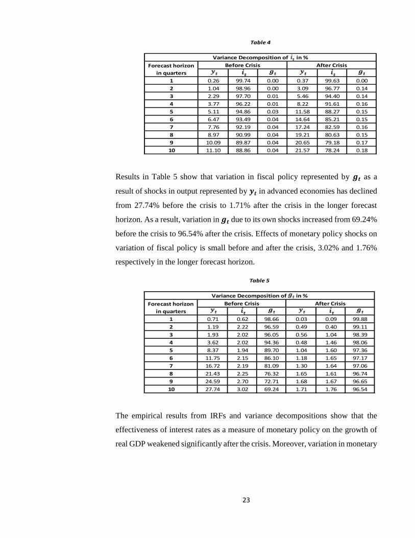
Results in Table 4 show that shocks in output represented by 𝒚𝒕 have triggered

more usage of monetary policy in advanced economies after the crisis to stabilize

the output which is explained by increase in variation of 𝒊𝒕 due to 𝒚𝒕 in the longer

forecast horizon from 11.10% before the crisis to 21.57% after the crisis. As a

result, variation in 𝒊𝒕 due to its own shocks decreased from 88.86% before crisis

to 78.24% after the crisis. Effects of fiscal policy shocks on variation of monetary

policy are insignificant before and after the crisis, 0.04% and 0.18% respectively

in the longer forecast horizon.

1 100.00 0.00 0.00 100.00 0.00 0.00

2 99.57 0.35 0.08 99.93 0.07 0.00

3 98.05 1.28 0.67 99.87 0.08 0.05

4 96.85 2.62 0.53 99.47 0.41 0.12

5 94.86 4.67 0.47 99.36 0.52 0.12

6 91.91 7.67 0.42 99.24 0.62 0.13

7 89.17 10.19 0.64 99.12 0.68 0.20

8 86.42 12.81 0.78 98.86 0.68 0.46

9 83.87 15.19 0.94 98.71 0.68 0.61

10 81.61 17.16 1.22 98.57 0.68 0.75

Table 3

Forecast horizon

in quarters

Before Crisis After Crisis

Variance Decomposition of in %

23

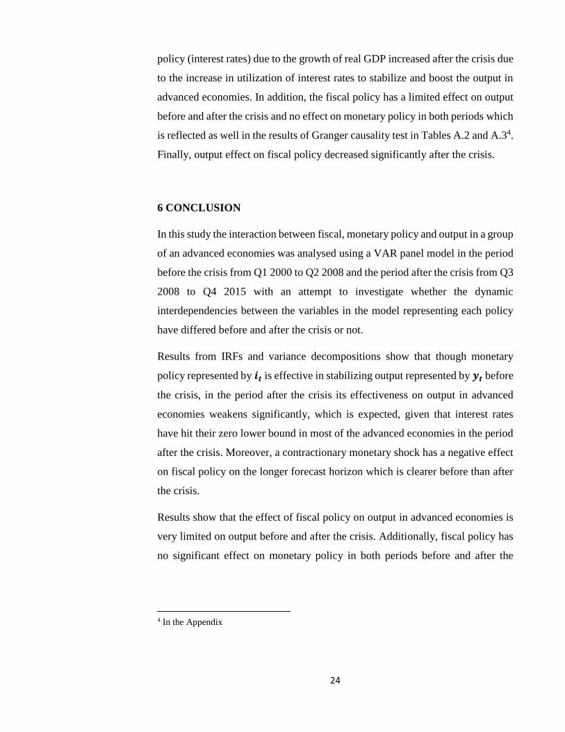
Results in Table 5 show that variation in fiscal policy represented by 𝒈𝒕 as a

result of shocks in output represented by 𝒚𝒕 in advanced economies has declined

from 27.74% before the crisis to 1.71% after the crisis in the longer forecast

horizon. As a result, variation in 𝒈𝒕 due to its own shocks increased from 69.24%

before the crisis to 96.54% after the crisis. Effects of monetary policy shocks on

variation of fiscal policy is small before and after the crisis, 3.02% and 1.76%

respectively in the longer forecast horizon.

The empirical results from IRFs and variance decompositions show that the

effectiveness of interest rates as a measure of monetary policy on the growth of

real GDP weakened significantly after the crisis. Moreover, variation in monetary

1 0.26 99.74 0.00 0.37 99.63 0.00

2 1.04 98.96 0.00 3.09 96.77 0.14

3 2.29 97.70 0.01 5.46 94.40 0.14

4 3.77 96.22 0.01 8.22 91.61 0.16

5 5.11 94.86 0.03 11.58 88.27 0.15

6 6.47 93.49 0.04 14.64 85.21 0.15

7 7.76 92.19 0.04 17.24 82.59 0.16

8 8.97 90.99 0.04 19.21 80.63 0.15

9 10.09 89.87 0.04 20.65 79.18 0.17

10 11.10 88.86 0.04 21.57 78.24 0.18

Table 4

Forecast horizon

in quarters

Before Crisis After Crisis

Variance Decomposition of in %

1 0.71 0.62 98.66 0.03 0.09 99.88

2 1.19 2.22 96.59 0.49 0.40 99.11

3 1.93 2.02 96.05 0.56 1.04 98.39

4 3.62 2.02 94.36 0.48 1.46 98.06

5 8.37 1.94 89.70 1.04 1.60 97.36

6 11.75 2.15 86.10 1.18 1.65 97.17

7 16.72 2.19 81.09 1.30 1.64 97.06

8 21.43 2.25 76.32 1.65 1.61 96.74

9 24.59 2.70 72.71 1.68 1.67 96.65

10 27.74 3.02 69.24 1.71 1.76 96.54

Table 5

Variance Decomposition of in %

Before Crisis After Crisis Forecast horizon

in quarters

24

policy (interest rates) due to the growth of real GDP increased after the crisis due

to the increase in utilization of interest rates to stabilize and boost the output in

advanced economies. In addition, the fiscal policy has a limited effect on output

before and after the crisis and no effect on monetary policy in both periods which

is reflected as well in the results of Granger causality test in Tables A.2 and A.34.

Finally, output effect on fiscal policy decreased significantly after the crisis.

6 CONCLUSION

In this study the interaction between fiscal, monetary policy and output in a group

of an advanced economies was analysed using a VAR panel model in the period

before the crisis from Q1 2000 to Q2 2008 and the period after the crisis from Q3

2008 to Q4 2015 with an attempt to investigate whether the dynamic

interdependencies between the variables in the model representing each policy

have differed before and after the crisis or not.

Results from IRFs and variance decompositions show that though monetary

policy represented by 𝒊𝒕 is effective in stabilizing output represented by 𝒚𝒕 before

the crisis, in the period after the crisis its effectiveness on output in advanced

economies weakens significantly, which is expected, given that interest rates

have hit their zero lower bound in most of the advanced economies in the period

after the crisis. Moreover, a contractionary monetary shock has a negative effect

on fiscal policy on the longer forecast horizon which is clearer before than after

the crisis.

Results show that the effect of fiscal policy on output in advanced economies is

very limited on output before and after the crisis. Additionally, fiscal policy has

no significant effect on monetary policy in both periods before and after the

4 In the Appendix

25

crisis, which is reinforced by the results of Granger causality test which indicates

that 𝒈𝒕 does not cause 𝒊𝒕.

Furthermore, the results show that following an output shock in advanced

economies monetary policy reacted in a countercyclical manner before and after

the crisis, though as mentioned earlier the effectiveness weakens after the crisis.

Yet fiscal policy responds in an expansionary manner to a positive output shock

before the crisis, however, after the crisis the response to the same effect is weak,

i.e., the response is nearly absent.

Overall, it can be concluded that monetary policy in advanced economies is more

effective on output before the crisis and fiscal policy does not affect output

significantly whether before or after the crisis. Moreover, shocks in output lead

to changes in monetary policy before and after the crisis, however, changes in

fiscal policy as a result of output shocks are more significant in the period before

the crisis.

Finally, this study can be extended by taking into consideration some additional

aspects. One of those aspects that can be taken into consideration is introducing

variables that capture government revenues as an additional measure of fiscal

policy from the revenue side. Moreover, another extension to the study that is

associated with the fiscal policy side is to split both discretionary and non-

discretionary components (automatic stabilizers) of fiscal policy and investigate

how the interaction between fiscal and monetary policy might result in different

macroeconomic effects.

Further insights can be generated as well by introducing a variable such as growth

in base money that captures how the unconventional monetary policy measures

that were implemented after the crisis in the advanced economies such as

quantitative easing might have affected the interaction between fiscal, monetary

policy and output.

26

References

Alesina, A., & Tabellini, G. (1987). rules and discretion with noncoordinated

monetary and fiscal policies. Economic Inquiry, 25(4), 619-630.

doi:10.1111/j.1465-7295.1987.tb00764.x.

Arestis, P. (2015). Coordination of fiscal with monetary and financial stability

policies can better cure unemployment. Review of Keynesian Economics, 3(2),

233-247.

Arestis, P., & Sawyer, M. (2004a). On the effectiveness of monetary policy and

of fiscal policy. Review of Social Economy, 62(4), 441-463.

doi:10.1080/0034676042000296218.

Arestis, P., & Sawyer, M. (2004b). Re-examining monetary and fiscal policy for

the 21st century. Cheltenham: Edward Elgar Publishing.

doi:10.4337/9781845423339.

Arestis, P., & Sawyer, M. (2012). The 'new economics' and policies for financial

stability. International Review of Applied Economics, 26(2), 147-160.

doi:10.1080/02692171.2011.640314.

Blanchard, O. (2011a). The Future of Macroeconomic Policy: Nine Tentative

Conclusions. iMF direct The International Monetary Fund’s Global Economic

Forum. Retrieved from https://blog-imfdirect.imf.org/2011/03/13/future-of-

macroeconomic-policy/

Blanchard, O. (2011b). Rewriting the Macroeconomists’ Playbook in the Wake

of the Crisis. iMF direct The International Monetary Fund’s Global Economic

Forum. Retrieved from https://blog-imfdirect.imf.org/2011/03/04/2662/

Blanchard, O. (2012). Monetary Policy in the Wake of the Crisis, in O.

Blanchard, D. Romer, A. M. Spence & J. E. Stiglitz (Ed), In the Wake of the

Crisis: Leading Economists Reassess Economic Policy (pp. 7-13). Cambridge,

Mass: MIT Press.

Blanchard, O., Dell'Ariccia, G., & Mauro, P. (2010). Rethinking

macroeconomic policy. Journal of Money, Credit and Banking, 42(1), 199-215.

doi:10.1111/j.1538-4616.2010.00334.x.

Blanchard, O., Dell'Ariccia, G., & Mauro, P. (2013). Rethinking Macro Policy

II: Getting Granular. IMF Staff Discussion Notes, 13(03), 1-25.

http://dx.doi.org/10.5089/9781484363478.006

27

Blanchard, O., & Perotti, R. (2002). An empirical characterization of the dynamic

effects of changes in government spending and taxes on output. The Quarterly

Journal of Economics, 117(4), 1329-1368. doi:10.1162/003355302320935043.

Blinder, A. S. (1982). Issues in the coordination of monetary and fiscal policy

(NBER working paper No. 982). Cambridge, Mass: National Bureau of

Economic Research.

Bouis, R., Rawdanowicz, L., Renne, J., Watanabe, S., & Christensen, A. K.

(2013). The effectiveness of monetary policy since the onset of the financial crisis.

(OECD Economic Department Working Paper no 1081). OECD Publishing.

Caldara, D., & Kamps, C. (2008). What are the effects of fiscal policy shocks? A

VAR-based comparative analysis (Working Paper Series No. 877). Frankfurt Am

Main: European Central Bank.

Canova, F., & Ciccarelli, M. (2013). Panel Vector Autoregressive Models: A

Survey. VAR Models in Macroeconomics–New Developments and Applications:

Essays in Honor of Christopher A. Sims (Advances in Econometrics, Volume 32)

Emerald Group Publishing Limited, 32, 205-246.

Coric, T., Simovic, H., & Deskar-Skrbic, M. (2015). Monetary and fiscal policy

mix in a small open economy: The case of croatia. Ekonomska Istrazivanja,

28(1), 407-421. doi:10.1080/1331677X.2015.1059073.

Eggertsson, G. B. (2006). Fiscal multipliers and policy coordination. Staff

Report, Federal Reserve Bank of New York, 241.

Friedman, M. (1948). A monetary and fiscal framework for economic stability.

The American Economic Review, 38(3), 245-264.

Gujarati, D. N. (2015). Econometrics by example (2nd ed.). London: Palgrave.

Gujarati, D. N. (2016). Basic econometrics (6th ed.). Singapore: McGraw-Hill.

Hutchison, M. M., Noy, I., & Wang, L. (2010). Fiscal and monetary policies and

the cost of sudden stops. Journal of International Money and Finance, 29(6), 1-

15. doi:10.1016/j.jimonfin.2009.12.005.

Indrawati, S. M. (2012). Fiscal policy responses to economic crisis: Perspective

from an emerging market, in O. Blanchard, D. Romer, A. M. Spence & J. E.

Stiglitz (Ed), In the Wake of the Crisis: Leading Economists Reassess Economic

Policy (pp. 67-71). Cambridge, Mass: MIT Press.

28

Laurens, B., & De La Piedra, E. (1998). Coordination of Monetary and Fiscal

Policies. IMF Working Papers, 98(25), 1-32.

http://dx.doi.org/10.5089/9781451844238.001

Li, J. (2013). The effectiveness of fiscal and monetary policy responses to twin

crises. Applied Economics, 45(27), 3904-3913.

Lutkepohl, H. (2005). New introduction to multiple time series analysis. Berlin:

Springer.

Mates, N. (2011). Fiscal policy: Lessons from the global crisis. Croatian

Economic Survey, 13(1), 5-56.

Mishkin, F. S. (2009). Is monetary policy effective during financial crises? The

American Economic Review, 99(2), 573-577. doi:10.1257/aer.99.2.573.

Mishkin, F. S. (2011). Monetary policy strategy: lessons from the crisis (NBER

working paper No. 16755). Cambridge, Mass: National Bureau of Economic

Research.

Mitreska, A., Kadievska Vojnovic, M., Georgievska, L., Jovanovic, B., &

Petkovska, M. (2010). Did the Crisis Change It All? Evidence from Monetary

and Fiscal Policy (Working Paper November 2010). National bank of the

Republic of Macedonia.

Muscatelli, A., Tirelli, P., & Trecroci, C. (2002). Monetary and fiscal policy

interactions over the cycle: Some empirical evidence (CESifo Working Paper

No. 817).

Niemann, S., & Hagen, J. (2008). Coordination of monetary and fiscal policies:

A fresh look at the issue. Swedish Economic Policy Review, 15(1), 89-124.

Petrevski, G., Bogoev, J., & Tevdovski, D. (2016). Fiscal and monetary policy

effects in three south eastern european economies. Empirical Economics, 50(2),

415-441. doi:10.1007/s00181-015-0932-0.

Reinhart, C. M., & Reinhart, V. R. (2010). After the fall (NBER working paper

No. 16334). Cambridge, Mass: National Bureau of Economic Research.

Romer, D. (2012). What Have We Learned about Fiscal Policy from the

Crisis?, in O. Blanchard, D. Romer, A. M. Spence & J. E. Stiglitz (Ed), In the

Wake of the Crisis: Leading Economists Reassess Economic Policy (pp. 57-66).

Cambridge, Mass: MIT Press.

29

Sargent, T. J., & Wallace, N. (1981). Some unpleasant monetarist arithmetic.

Federal Reserve Bank of Minneapolis. Quarterly Review - Federal Reserve Bank

of Minneapolis, 5(3), 1-17.

Semmler, W., & Zhang, W. (2004). Monetary and fiscal policy interactions in

the euro area. Empirica, 31(2), 205-227. doi:10.1007/s10633-004-1076-1.

Senbet, D. (2011). the relative impact of fiscal versus monetary actions on output:

A vector autoregressive (VAR) approach. Business and Economic Journal, 25,

1-11.

Sims, C. A. (1980). Macroeconomics and reality. Econometrica, 48(1), 1-48.

Stiglitz, J. (2012). Macroeconomics, Monetary Policy, and the Crisis, in O.

Blanchard, D. Romer, A. M. Spence & J. E. Stiglitz (Ed), In the Wake of the

Crisis: Leading Economists Reassess Economic Policy (pp. 31-42). Cambridge,

Mass: MIT Press.

30

Appendix

ID Country

1 Australia2 Austria3 Belgium4 Canada5 Czech Republic6 Denmark7 Estonia8 Finland9 France10 Germany11 Greece12 Iceland13 Ireland14 Italy15 Latvia16 Lithuania17 Netherlands18 Norway19 Portugal20 Singapore21 Slovak Republic22 Slovenia23 Spain24 Sweden25 United Kingdom26 United States

Table A.1: List of advanced countries in the panel dataset

Independent Variables Before Crisis After Crisis

Chi-sq Chi-sq

47.559** 11.319**

13.328** 4.354

** indicates presence of Causality

Dependent variable:

Table A.2: Granger Causality Test results

31

Independent Variables Before Crisis After Crisis

Chi-sq Chi-sq

11.581** 65.600**

0.213 7.739

** indicates presence of Causality

Independent Variables Before Crisis After Crisis

Chi-sq Chi-sq

57.544** 19.961**

19.078** 12.805**

** indicates presence of Causality

Table A.4: Granger Causality Test results

Dependent variable:

Dependent variable:

Table A.3: Granger Causality Test results