research challenges in process systems engineering and...

Research Challenges in Process Systems Engineering and Overview of Mathematical Programming

Ignacio E. GrossmannCenter for Advanced Process Decision-making (CAPD)

Department of Chemical EngineeringCarnegie Mellon University

Pittsburgh, PA 15213, U.S.A.

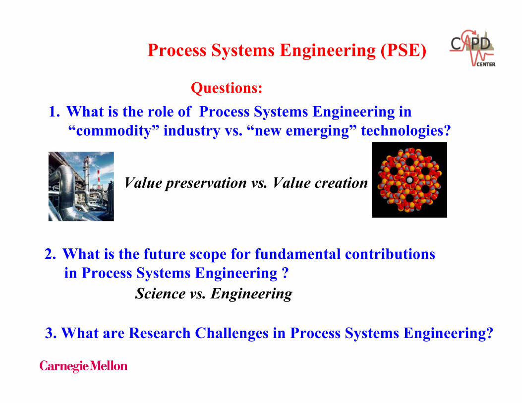
Questions:1. What is the role of Process Systems Engineering in

“commodity” industry vs. “new emerging” technologies?

2. What is the future scope for fundamental contributionsin Process Systems Engineering ?

Process Systems Engineering (PSE)

Value preservation vs. Value creation

Science vs. Engineering

3. What are Research Challenges in Process Systems Engineering?

Changes in the Chemical Industry

From Marcinowski (2006)

ExxonMobil $208.7 $237 $359ChevronTexaco 99.7 120 193

Revenues of major U.S. companies (billions)(2001) (2003) (2005)

Johnson & Johnson 32.3 41.8 50.5Merck 21.2 22.4 22.0Bristol-Myers Squibb 21.7 18.6 19.2

Procter & Gamble 39.2 43.4 56.7

Dow 27.8 32.6 46.3DuPont 26.8 30.2 25.3

Amgen 4.0 8.4 12.4 Genentech 1.7 3.3 5.5

Economics of Chemical Enterprise

Value preservation vs. Value Creation

Move from Engineering to Science

Papers U.S.Fluid Mechanics, Transport Phenomena 57 18Reactors, Kinetics, Catalysis 56 21Process Systems Engineering 51 22Separations 37 11Particle Technology, Fluidization 28 11Thermodynamics 19 2Materials, Interfaces, Electrochemical Phenomena 21 9Environmental, Energy Engineering 16 8Bioeng., Food, Natural Products 9 5

Total 294 107

Distribution Research Papers AIChE Journal 2005

=> Only 36% papers involve US-based authors

Only 15% from top 25 U.S. schools

Observations

Trade-offs: Value preservation vs. Value growthChemicals/Fuels vs. Pharmaceutical/Biotechnology

Major real world challenges Globalization, energy, environment, health

=> Need expand scope of Process Systems Engineering

Research trend away from Chemical EngineeringScience vs Engineering

Expanding the Scope of Process Systems Engineering

(Grossmann & Westerberg, 2000; Marquardt et al, 1998)

Major Research Challenges

I. Product and Process Design

III. Enterprise-wide Optimization

II. Energy and Sustainability

What is science base for PSE?

Numerical analysis => Simulation

Mathematical Programming => Optimization

Systems and Control Theory => Process Control

Computer Science => Advanced Info./Computing

Management Science => Operations/Business

Math Programming & Control Theory “competitive” advantage

MotivationDesign, operations and control problems involve decision-makingover a large number of alternatives for selecting “best” solution

- Configurations (discrete variables)- Parameter values (continuous variables)

Motivation Math Programming

Challenges:How to model optimization problems?How to solve large-scale models?How to avoid local solutions?How to handle uncertainties?

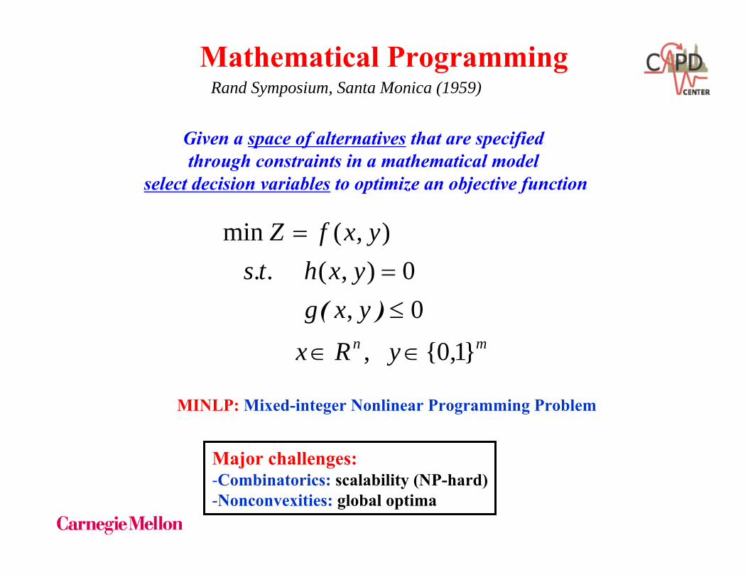
Mathematical Programming

Given a space of alternatives that are specified through constraints in a mathematical model

select decision variables to optimize an objective function

Rand Symposium, Santa Monica (1959)

mn yRxyxgyx hts

yxfZ

1,0,0,

0),(..),(min

∈∈

≤=

=

)(

MINLP: Mixed-integer Nonlinear Programming Problem

Major challenges:-Combinatorics: scalability (NP-hard)-Nonconvexities: global optima

nRxxfZ

∈

=

)(min

nRxx htsxfZ

∈

==

)(

0..

)(min

Newton (1664)

Lagrange (1778)

Solution of inequalities Fourier (1826)Solution of linear equations Gauss (1826)Solution of inequality systems Farkas (1902)

Classical Optimization

x1

x2

x1

x2

Linear Programming Kantorovich (1939), Dantzig (1947)

Nonlinear Programming Karush (1939), Kuhn, A.W.Tucker (1951)

Integer Programming R. E. Gomory (1958)

y1

y2

Modern Optimization

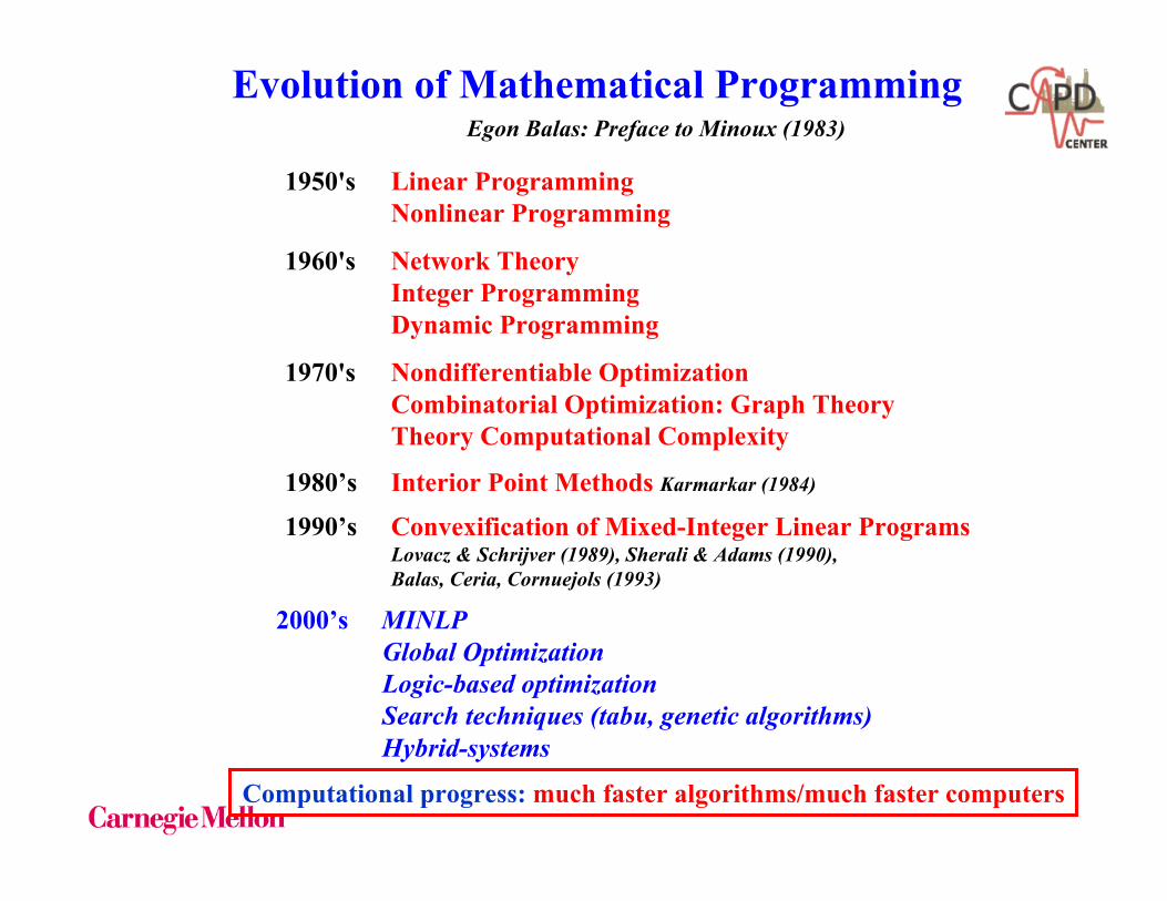
1950's Linear ProgrammingNonlinear Programming

1960's Network TheoryInteger ProgrammingDynamic Programming

1970's Nondifferentiable OptimizationCombinatorial Optimization: Graph TheoryTheory Computational Complexity

Evolution of Mathematical ProgrammingEgon Balas: Preface to Minoux (1983)

1980’s Interior Point Methods Karmarkar (1984)

1990’s Convexification of Mixed-Integer Linear ProgramsLovacz & Schrijver (1989), Sherali & Adams (1990),Balas, Ceria, Cornuejols (1993)

2000’s MINLPGlobal OptimizationLogic-based optimizationSearch techniques (tabu, genetic algorithms)Hybrid-systems

Computational progress: much faster algorithms/much faster computers

Progress in Linear Programming

AlgorithmsPrimal simplex in 1987 (XMP) versusBest(primal,dual,barrier) 2002 (CPLEX 7.1) 2400x

Increase in computational speed from 1987 to 2002Bixby-ILOG (2002)

MachinesSun 3/150Pentium 4, 1.7GHz 800x

Net increase: Algorithm * Machine ~ 1 900 000x

Two million-fold increase in speed!!

For 50,000 constraint LP model

Contributions by Chemical Engineers to Mathematical ProgrammingLarge-scale nonlinear programmingSQP algorithmsInterior Point algorithms

Mixed-integer nonlinear programmingOuter-approximation algorithmExtended-Cutting Plane MethodGeneralized Disjunctive Programming

Global optimizationα-Branch and BoundSpatial branch and bound methods

Optimal control problemsNLP-based strategies

Optimization under UncertaintySim-OptParametric programming

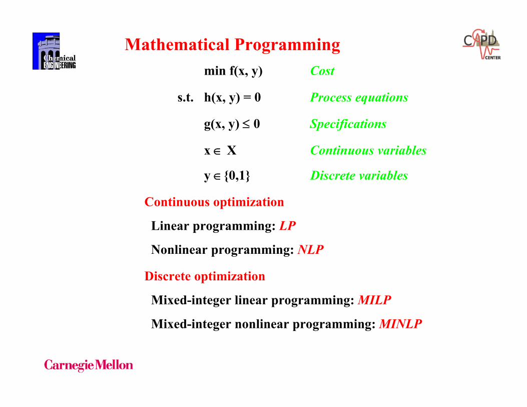
Mathematical Programming min f(x, y) Cost

s.t. h(x, y) = 0 Process equations

g(x, y) ≤ 0 Specifications

x ∈ X Continuous variables

y ∈0,1 Discrete variables

Continuous optimization

Linear programming: LP

Nonlinear programming: NLP

Discrete optimization

Mixed-integer linear programming: MILP

Mixed-integer nonlinear programming: MINLP

Modeling systems

Mathematical Programming

GAMS (Meeraus et al, 1997)

AMPL (Fourer et al., 1995)

AIMSS (Bisschop et al. 2000)

1. Algebraic modeling systems => pure equation models

2. Indexing capability => large-scale problems

3. Automatic differentiation => no derivatives by user

4. Automatic interface with LP/MILP/NLP/MINLP solvers

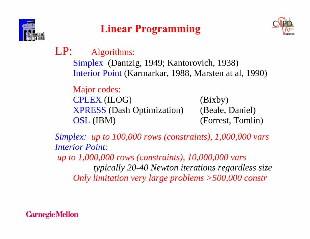
LP: Algorithms: Simplex (Dantzig, 1949; Kantorovich, 1938) Interior Point (Karmarkar, 1988, Marsten at al, 1990)

Major codes: CPLEX (ILOG) (Bixby) XPRESS (Dash Optimization) (Beale, Daniel) OSL (IBM) (Forrest, Tomlin)

Simplex: up to 100,000 rows (constraints), 1,000,000 varsInterior Point: up to 1,000,000 rows (constraints), 10,000,000 vars typically 20-40 Newton iterations regardless size Only limitation very large problems >500,000 constr

Linear Programming

MILP

Branch and Bound Beale (1958), Balas (1962), Dakin (1965)

Cutting planes Gomory (1959), Balas et al (1993)

Branch and cut Johnson, Nemhauser & Savelsbergh (2000)

"Good" formulation crucial! => Small LP relaxation gap Drawback: exponential complexity

0,1,0

min

≥∈≤+

+=

xydBxAyst

xbyaZ

m

TT

Theory for ConvexificationLovacz & Schrijver (1989), Sherali & Adams (1990),

Balas, Ceria, Cornuejols (1993)

Objective function

Constraints

LP (simplex) based

Modeling with MILP Note: linear constraints

3. Integer numbers

1. Multiple choiceAt least one

Exactly one

At most one

1

1

ii I

ii I

y

y∈

∈

=

≤

∑

∑

1ii I

y∈

≥∑

2. ImplicationIf select i then select kSelect i if and only if select k

00

i k

i k

y yy y

− ≤

− =

∑∑==

==N

kk

N

kk ykyn

11

1, also ∑=

=M

kk

k yn12 Fewer 0-1 variables

Weaker relaxation

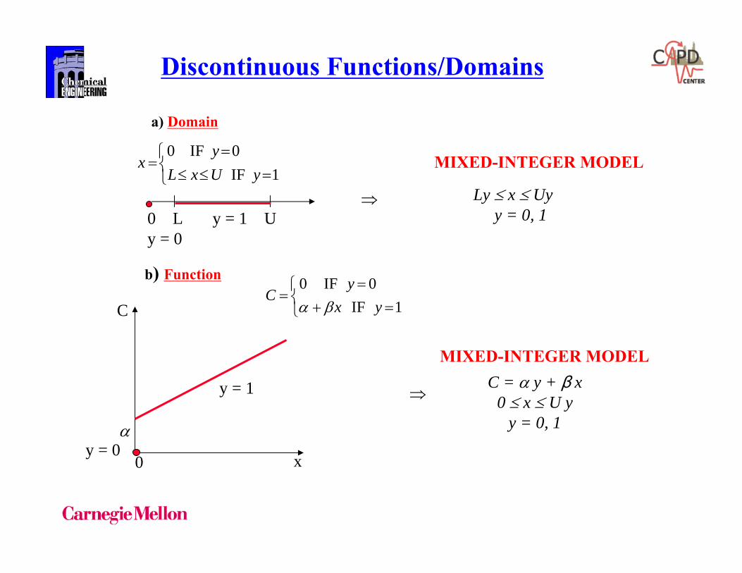
⇒ Ly ≤ x ≤ Uyy = 0, 1

MIXED-INTEGER MODEL

MIXED-INTEGER MODEL

Discontinuous Functions/Domains

⇒C = α y + β x

0 ≤ x ≤ U yy = 0, 1

0 L y = 1 Uy = 0

⎩⎨⎧

=≤≤=

=1 IF

0 IF0yUxL

yx

a) Domain

b) Function

⎩⎨⎧

=+=

=1 IF

0 IF0yx

yC

βα

y = 1

αy = 0

0 x

C

Simple Minded Approaches

Exhaustive EnumerationSOLVE LP’S FOR ALL 0-1 COMBINATIONS (2m)IF m = 5 32 COMBINATIONSIF m = 100 1030 COMBINATIONSIF m = 10,000 103000 COMBINATIONS

Relaxation and RoundingSOLVE MILP WITH 0 ≤ y ≤ 1If solution not integer round closestRELAXATION

Only special cases yield integer optimum (Assignment Problem)

Relaxed LP provides LOWER BOUND to MILP solution

Difference: Relaxation gap

ROUNDINGMay yield infeasible or suboptimal solution

y21

Integer Optimum

INFEASIBLE !

Rounded Infeasible0 0.5 1

0.5Relaxed optimum

Rounded feasible

y21

Integer Optimum

SUBOPTIMAL !

0 0.5 1

0.5Relaxed optimum

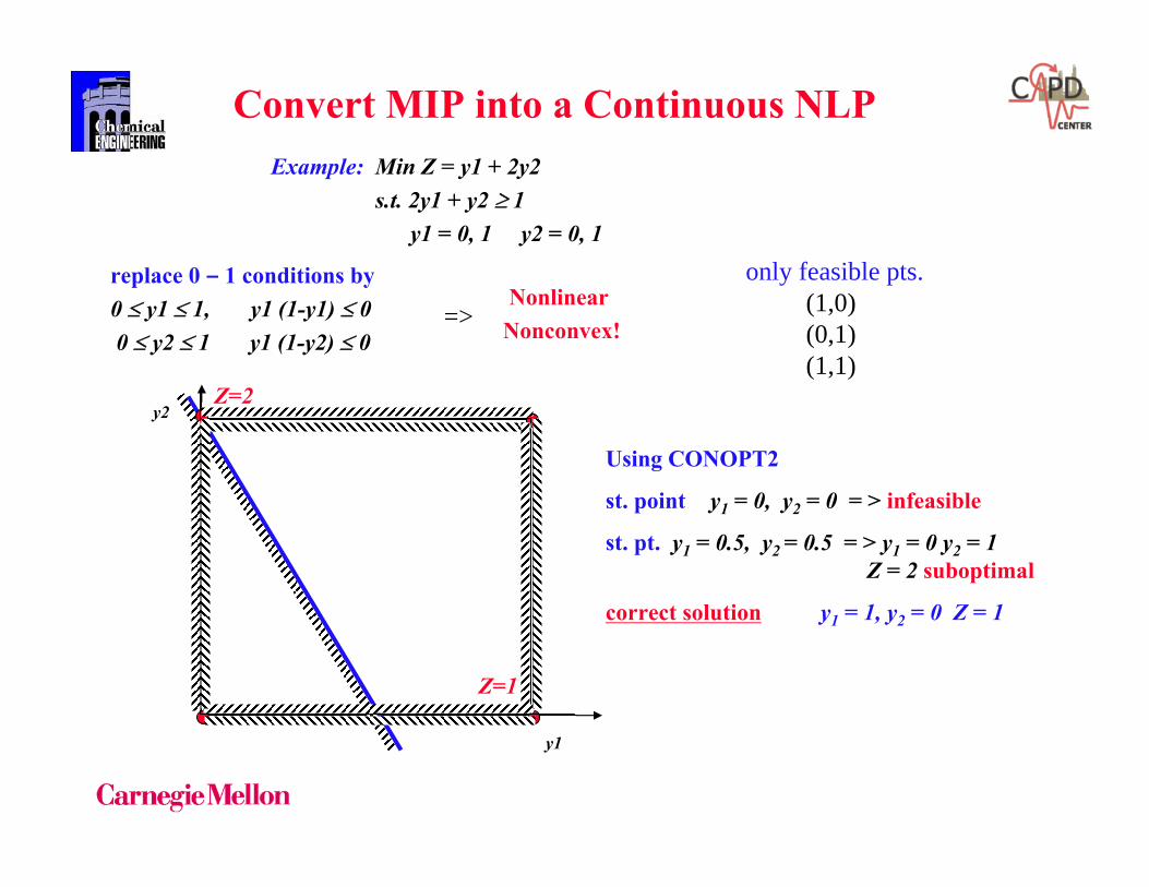
Convert MIP into a Continuous NLPExample: Min Z = y1 + 2y2

s.t. 2y1 + y2 ≥ 1y1 = 0, 1 y2 = 0, 1

replace 0 – 1 conditions by 0 ≤ y1 ≤ 1, y1 (1-y1) ≤ 0 0 ≤ y2 ≤ 1 y1 (1-y2) ≤ 0

Nonlinear Nonconvex!=>

y1

y2

only feasible pts.(1,0)(0,1)(1,1)

Using CONOPT2

st. point y1 = 0, y2 = 0 = > infeasible

st. pt. y1 = 0.5, y2 = 0.5 = > y1 = 0 y2 = 1Z = 2 suboptimal

correct solution y1 = 1, y2 = 0 Z = 1

Z=2

Z=1

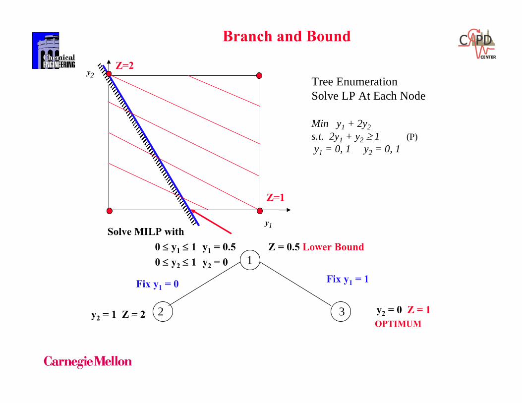
Branch and Bound

y1

y2 Tree EnumerationSolve LP At Each Node

Min y1 + 2y2s.t. 2y1 + y2 ≥ 1 (P)y1 = 0, 1 y2 = 0, 1

Solve MILP with0 ≤ y1 ≤ 1 y1 = 0.5 Z = 0.5 Lower Bound0 ≤ y2 ≤ 1 y2 = 0

Fix y1 = 1

y2 = 0 Z = 1OPTIMUM

1

32

Fix y1 = 0

y2 = 1 Z = 2

Z=2

Z=1

Major Solution Approaches MILP

I. EnumerationBranch and boundLand,Doig (1960) Dakin (1965)Basic idea: partition successively integer space to determine whether subregionscan be eliminated by solving relaxed LP problems

II. ConvexificationCutting planesGomory (1958) Crowder, Johnson, Padberg (1983), Balas, Ceria, Cornjuelos (1993)Basic idea: solve sequence relaxed LP subproblems by adding valid inequalitiesthat cut-off previous solutions

Remark- Branch and bound most widely used- Recent trend to integrate it with cutting planes

BRANCH-AND-CUT

Branch and BoundPartitioning Integer Space Performed with Binary Tree

Note: 15 nodes for 23=8 0-1 combinations

y1=1y1=0

y2=1y2=0

y3=0

y3=1

y2=0 y2=1

y3=0 y3=0 y3=0

y3=1 y3=1 y3=1

Root Node (LP Relaxation)

3,2,1,10 =≤≤ iyi

Node

Node k

Node k descendent node

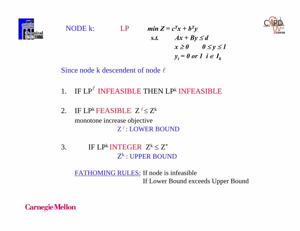
NODE k: LP min Z = cTx + bTys.t. Ax + By ≤ d

x ≥ 0 0 ≤ y ≤ 1yi = 0 or 1 i ∈ Ik

Since node k descendent of node

1. IF LP INFEASIBLE THEN LPk INFEASIBLE

2. IF LPk FEASIBLE Z ≤ Zk

monotone increase objective Z : LOWER BOUND

3. IF LPk INTEGER Zk ≤ Z*

Zk : UPPER BOUND

FATHOMING RULES: If node is infeasibleIf Lower Bound exceeds Upper Bound

“If sufficient care is exercised, it is now possible to solve MILP models of size approaching ‘large’ LP’s. Note, however, that ‘sufficient care’ is the operative phrase”. JOHN TOMLIN (1983)

Modeling of Integer Programs

HOW TO MODEL INTEGER CONSTRAINTS?Propositional LogicDisjunctions

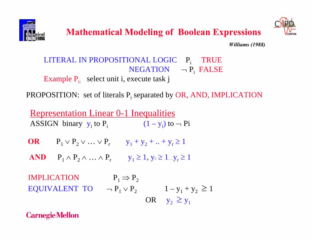
Mathematical Modeling of Boolean ExpressionsWilliams (1988)

LITERAL IN PROPOSITIONAL LOGIC Pi TRUENEGATION ¬ Pi FALSE

Example Pi: select unit i, execute task j

PROPOSITION: set of literals Pi separated by OR, AND, IMPLICATION

Representation Linear 0-1 InequalitiesASSIGN binary yi to Pi (1 – yi) to ¬ Pi

OR P1 ∨ P2 ∨ … ∨ Pr y1 + y2 + .. + yr ≥ 1

AND P1 ∧ P2 ∧ … ∧ Pr y1 ≥ 1, y2 ≥ 1, …yr ≥ 1

IMPLICATION P1 ⇒ P2

EQUIVALENT TO ¬ P1 ∨ P2 1 – y1 + y2 ≥ 1OR y2 ≥ y1

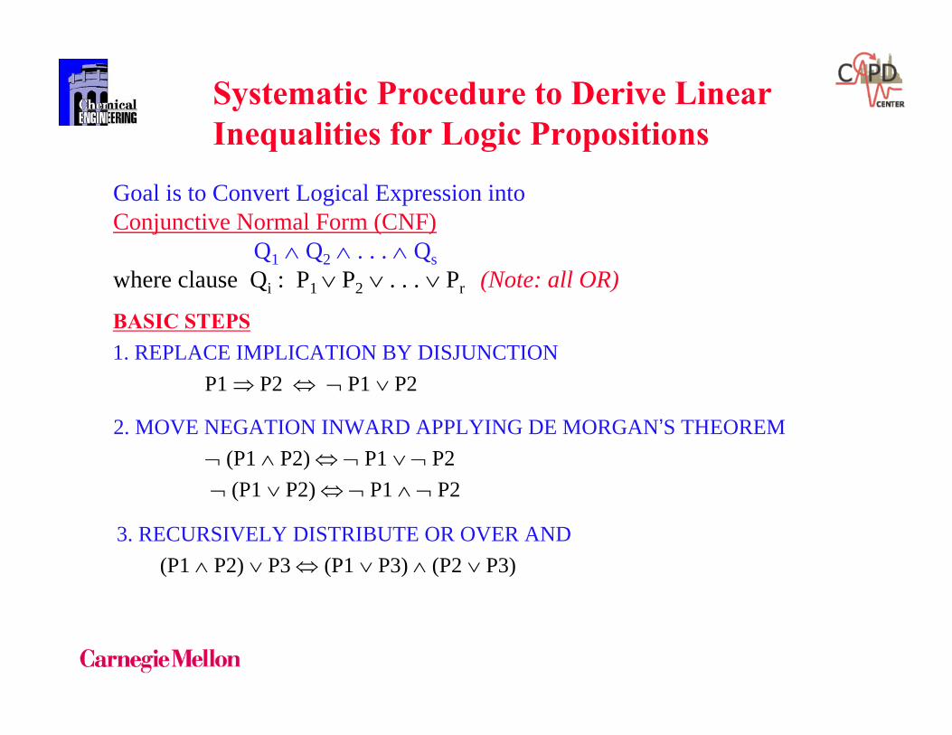
Systematic Procedure to Derive LinearInequalities for Logic Propositions

Goal is to Convert Logical Expression intoConjunctive Normal Form (CNF)

Q1 ∧ Q2 ∧ . . . ∧ Qswhere clause Qi : P1 ∨ P2 ∨ . . . ∨ Pr (Note: all OR)

3. RECURSIVELY DISTRIBUTE OR OVER AND(P1 ∧ P2) ∨ P3 ⇔ (P1 ∨ P3) ∧ (P2 ∨ P3)

BASIC STEPS1. REPLACE IMPLICATION BY DISJUNCTION

P1 ⇒ P2 ⇔ ¬ P1 ∨ P2

2. MOVE NEGATION INWARD APPLYING DE MORGAN’S THEOREM¬ (P1 ∧ P2) ⇔ ¬ P1 ∨ ¬ P2¬ (P1 ∨ P2) ⇔ ¬ P1 ∧ ¬ P2

EXAMPLEflash ⇒ dist ∨ absmemb ⇒ not abs ∧ comp

PF ⇒ PD ∨ PA (1)PM ⇒ ¬ PA ∧ PC (2)

(1) ¬ PF ∨ PD ∨ PA remove implication

1 – yF + yD + yA ≥ 1yD + yA ≥ yF

(2) ¬ PM ∨ (¬ PA ∧ Pc) remove implication

1 – yM + 1 – yA ≥ 1 1 – yM + yC ≥ 1yM + yA ≤ 1 yc ≥ yM

Verify: yF = 1 yD + yA ≥ 1 yF = 0 yD + yA ≥ 0yM = 1 ⇒ yA = 0 yC = 1

yD + yA ≥ yFyM + yA ≤ 1yC ≥ yM

(¬ PM ∨ ¬ PA) ∧ (¬ PM ∨ Pc) distribute OR over AND => CNF!

EXAMPLEInteger CutConstraint that is infeasible for integer point

yi = 1 i ∈ B yi = 0 i ∈ Nand feasible for all other integer points

1

1)1(

)()(

)]()[(

−≤−

≥+−

↓

∨¬

¬∧¬

∑∑

∑∑

∨∨

∧∧

∈∈

∈∈

∈∈

∈∈

BNi

iBi

i

Niii

Bi

iNiiBi

iNiiBi

yy

yy

yy

yy

Balas andJeroslow (1968)

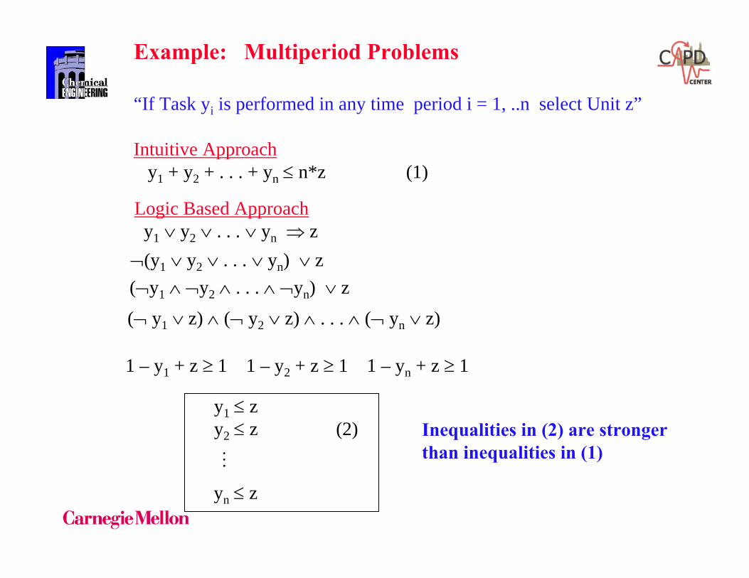
Example: Multiperiod Problems

“If Task yi is performed in any time period i = 1, ..n select Unit z”

Intuitive Approachy1 + y2 + . . . + yn ≤ n*z (1)

Logic Based Approachy1 ∨ y2 ∨ . . . ∨ yn ⇒ z

Inequalities in (2) are stronger than inequalities in (1)

¬(y1 ∨ y2 ∨ . . . ∨ yn) ∨ z

(¬ y1 ∨ z) ∧ (¬ y2 ∨ z) ∧ . . . ∧ (¬ yn ∨ z)

1 – y1 + z ≥ 1 1 – y2 + z ≥ 1 1 – yn + z ≥ 1

…yn ≤ z

y1 ≤ zy2 ≤ z (2)

(¬y1 ∧ ¬y2 ∧ . . . ∧ ¬yn) ∨ z

1

1

1

y1

y2

z

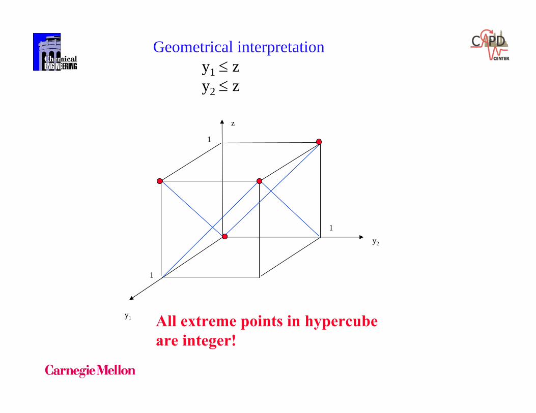
Geometrical interpretationy1 ≤ zy2 ≤ z

All extreme points in hypercubeare integer!

1

1

1

y1

y2

z

0.5

0.5

Geometrical interpretation

y1 + y2 ≤ 2z

Non-integer extreme pointsWeaker relaxation!

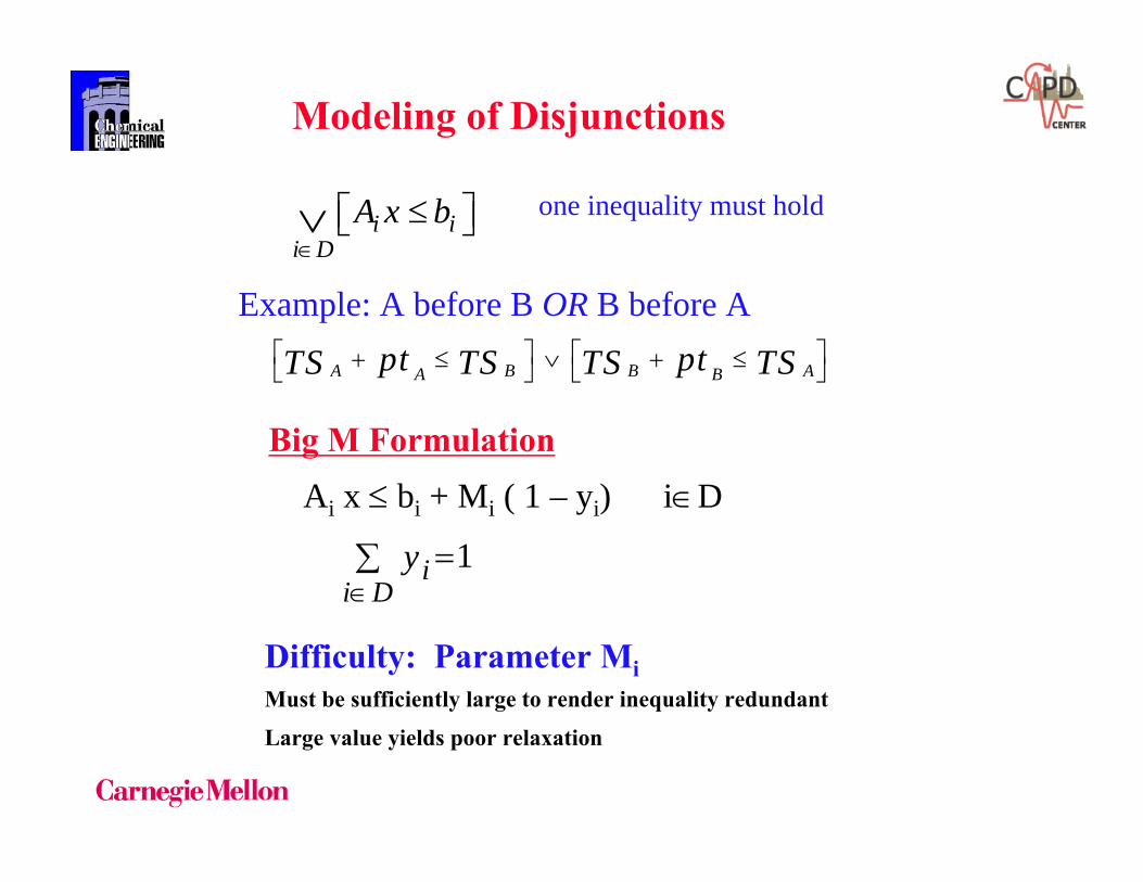
Modeling of Disjunctions

i ii D

A x b∈

≤⎡ ⎤⎣ ⎦∨ one inequality must hold

Example: A before B OR B before A

A B B AA Bpt ptTS TS TS TS⎡ ⎤ ⎡ ⎤+ ≤ ∨ + ≤⎣ ⎦ ⎣ ⎦

Big M FormulationAi x ≤ bi + Mi ( 1 – yi) i∈D

1=∑∈Di

iy

Difficulty: Parameter MiMust be sufficiently large to render inequality redundant

Large value yields poor relaxation

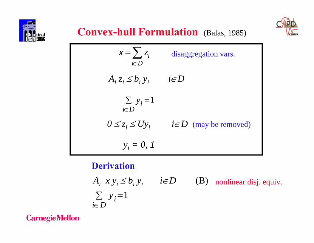
Convex-hull Formulation (Balas, 1985)

disaggregation vars.ii D

x z∈

= ∑

Ai zi ≤ bi yi i∈D

1=∑∈Di

iy

0 ≤ zi ≤ Uyi i∈D (may be removed)

yi = 0, 1

DerivationAi x yi ≤ bi yi i∈D (B)

1=∑∈Di

iynonlinear disj. equiv.

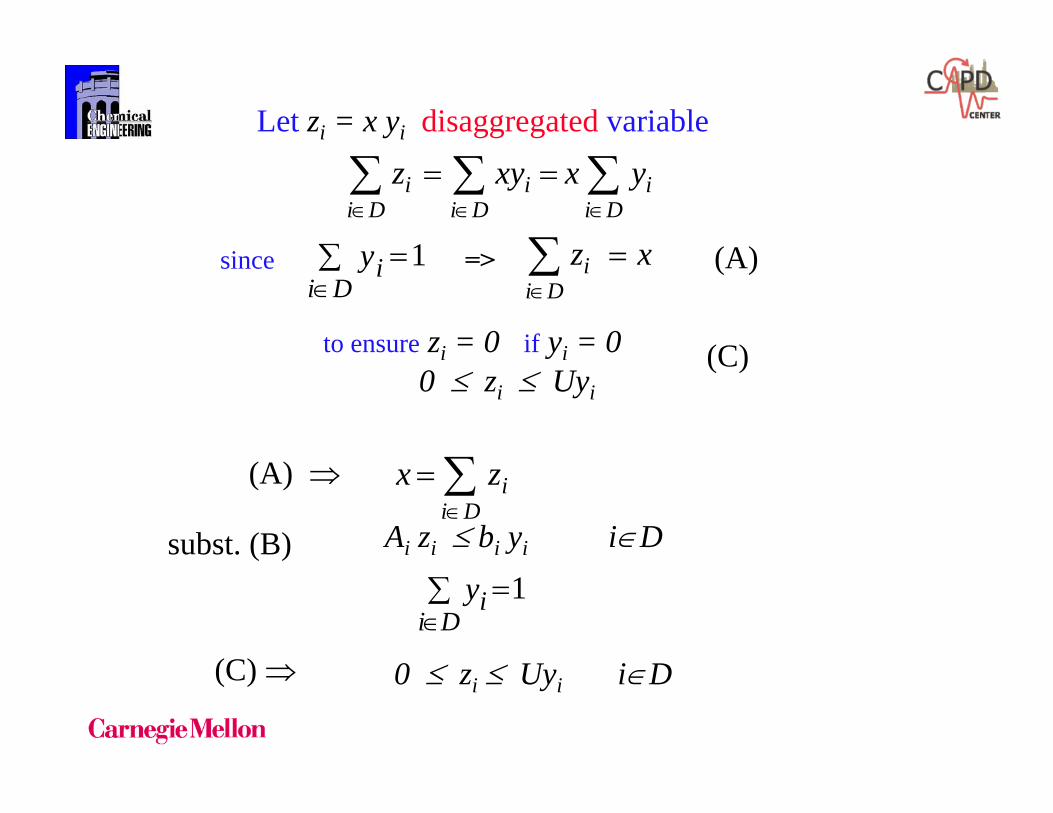
Let zi = x yi disaggregated variable

1=∑∈Di

iy

i i ii D i D i D

z xy x y∈ ∈ ∈

= =∑ ∑ ∑

(A)

to ensure zi = 0 if yi = 00 ≤ zi ≤ Uyi

(C)

(A) ⇒ ii D

x z∈

= ∑subst. (B) Ai zi ≤ bi yi i∈D

1=∑∈Di

iy

(C) ⇒ 0 ≤ zi ≤ Uyi i∈D

ii D

z x∈

=∑since =>

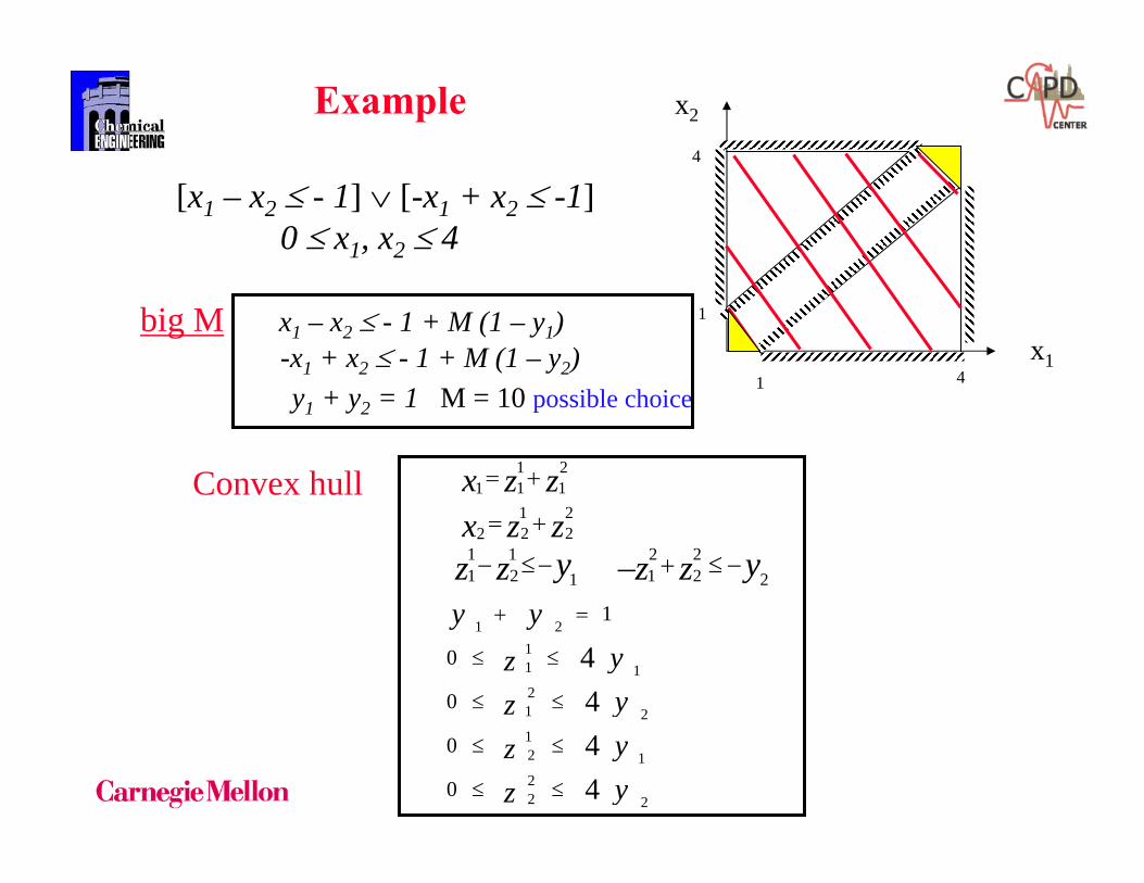
Example

[x1 – x2 ≤ - 1] ∨ [-x1 + x2 ≤ -1]0 ≤ x1, x2 ≤ 4

x2

x1

big M x1 – x2 ≤ - 1 + M (1 – y1)-x1 + x2 ≤ - 1 + M (1 – y2)y1 + y2 = 1 M = 10 possible choice

4

4

1

1

Convex hull 1 21 111 22 22

x z zx z z

= +

= +1 1 2 21 2 1 21 2y yz z z z− ≤− + ≤ −−

1 211 121 212 122 2

1

0

0

0

0

4444

y yyzyzyzyz

+ =

≤ ≤

≤ ≤

≤ ≤

≤ ≤

NLP: Algorithms (variants of Newton's method for solving KKT conditions)

Sucessive quadratic programming (SQP) (Han 1976; PowellReduced gradient Interior Point Methods

Major codes: MINOS (Murtagh, Saunders, 1978, 1982)

CONOPT (Drud, 1994) SQP: SNOPT (Murray, 1996) OPT (Biegler, 1998) IP: IPOPT (Wachter, Biegler, 2002) www.coin-or.org Typical sizes: 50,000 vars, 50,000 constr. (unstructured) 500,000 vars (few degrees freedom) Convergence: Good initial guess essential (Newton's) Nonconvexities: Local optima, non-convergence

Nonlinear Programming

MINLP

f(x,y) and g(x,y) - assumed to be convex and bounded over X. f(x,y) and g(x,y) commonly linear in y

,1,0|,,|

, 0),( ..

),(min

aAyyyYbBxxxxRxxX

YyXxyx gts

yxfZ

m

ULn

≤∈=≤≤≤∈=

∈∈≤

=

• Mixed-Integer Nonlinear Programming

Objective Function

Inequality Constraints

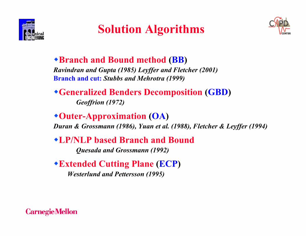
Branch and Bound method (BB)Ravindran and Gupta (1985) Leyffer and Fletcher (2001)Branch and cut: Stubbs and Mehrotra (1999)

Generalized Benders Decomposition (GBD)Geoffrion (1972)

Outer-Approximation (OA)Duran & Grossmann (1986), Yuan et al. (1988), Fletcher & Leyffer (1994)

LP/NLP based Branch and BoundQuesada and Grossmann (1992)

Extended Cutting Plane (ECP)Westerlund and Pettersson (1995)

Solution Algorithms

Basic NLP subproblems

a) NLP Relaxation Lower bound

kFU

kii

kFL

kii

R

j

kLB

Iiy

Iiy

YyXx

JjyxgtsyxfZ

∈≥

∈≤

∈∈

∈≤=

β

α

(NLP1),

0),(..),(min

b) NLP Fixed yk Upper bound

Xx

Jjyxgts

yxfZk

j

kkU

∈

∈≤

=

0),(..

),(min

(NLP2)

c) Feasibility subproblem for fixed yk.

1,

),(..min

RuXx

Jjuyxgtsu

kj

∈∈

∈≤ (NLPF)

Infinity-norm

Cutting plane MILP master (Duran and Grossmann, 1986)

Based on solution of K subproblems (xk, yk) k=1,...K Lower Bound M-MIP

YyXx

Kk

Jjyyxx

yxgyxg

yyxx

yxfyxfst

Z

k

kTkk

jkk

j

k

kTkkkk

KL

∈∈

=

⎪⎪

⎭

⎪⎪

⎬

⎫

∈≤⎥⎥⎦

⎤

⎢⎢⎣

⎡

−

−∇+

⎥⎥⎦

⎤

⎢⎢⎣

⎡

−

−∇+≥

=

,

,...1

0),(),(

),(),(

min

α

α

Notes:

a) Point (xk, yk) k=1,...K normally from NLP2

b) Linearizations accumulated as iterations K increase

c) Non-decreasing sequence lower bounds

X

f(x)

x

x

1

2x

1

x2

Linearizations and Cutting Planes

Underestimate Objective Function

Overestimate Feasible Region

ConvexObjective

ConvexFeasibleRegion

XX1 2

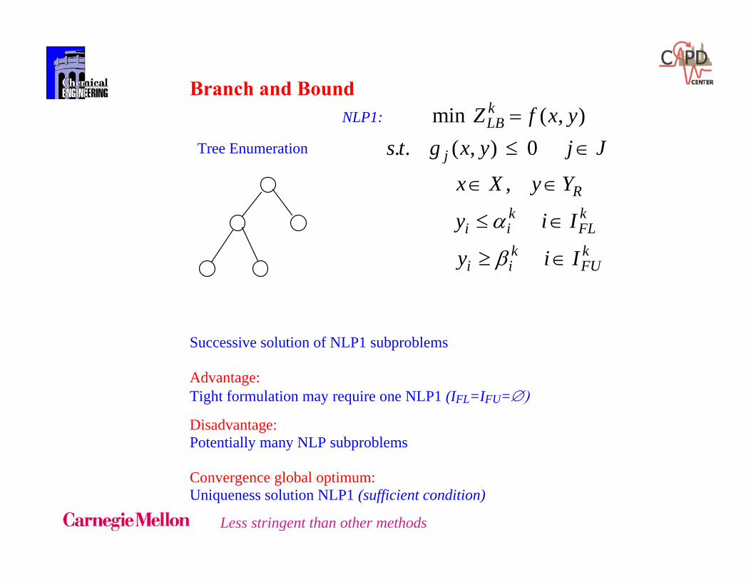
Branch and Bound

NLP1:

min ZLBk = f(x,y)

Tree Enumeration s.t. g j(x,y) < 0 j∈J

x∈X , y∈YRyi < αi

k i∈IFLk

yi > β ik i∈IFU

k

Successive solution of NLP1 subproblems Advantage: Tight formulation may require one NLP1 (IFL=IFU=∅)

Disadvantage: Potentially many NLP subproblems Convergence global optimum: Uniqueness solution NLP1 (sufficient condition)

Less stringent than other methods

min ( , ). . ( , ) 0

,

kLB

j

Rk k

i i FLk k

i i FU

Z f x ys t g x y j J

x X y Y

y i I

y i I

α

β

=≤ ∈

∈ ∈

≤ ∈

≥ ∈

Outer-Approximation Alternate solution of NLP and MIP problems:

NLP2

M-MIP

NLP2: min ZU

k = f(x,yk)

s.t. g j( x,yk) < 0 j∈J

x∈X

M-MIP: min ZLK = α

s.t α > f xk,yk + ∇f xk,yk T x–xk

y–yk

g xk,yk + ∇gj xk,yk T x–xk

y–yk < 0 j∈Jkk=1..K

x∈ X, y∈Y , α∈ R1

Property. Trivially converges in one iteration if f(x,y) and g(

- If infeasible NLP solution of feasibility NLP-F required to guarantee convergence.

Xx

Jjyxgts

yxfZk

j

kkU

∈

∈≤

=

0),(..

),(min

min

( , ) ( , )

1,...

( , ) ( , ) 0

,

KL

kk k k k T

k

kk k k k T k

j j k

Z

x xst f x y f x y

y yk K

x xg x y g x y j J

y y

x X y Y

α

α

=

⎫⎡ ⎤−⎪≥ + ∇ ⎢ ⎥⎪−⎢ ⎥⎣ ⎦ ⎪ =⎬

⎡ ⎤− ⎪+ ∇ ≤ ∈⎢ ⎥ ⎪

−⎢ ⎥ ⎪⎣ ⎦ ⎭∈ ∈

x,y) are linear

Upper bound

Lower bound

Generalized Benders Decomposition Benders (1962), Geoffrion (1972)

Particular case of Outer-Approximation as applied to (P1)

1. Consider Outer-Approximation at (xk, yk)

α > f xk,yk + ∇f xk,yk T x–xk

y–yk

g xk,yk + ∇gj xk,yk T x–xk

y–yk < 0 j∈Jk

(1)

2. Obtain linear combination of (1) using Karush-Kuhn- Tucker multipliers μk and eliminating x variables

α > f xk,yk + ∇yf xk,yk T y–yk

(2)

+ μk T g xk,yk + ∇yg xk,yk T y–yk

Lagrangian cut

Remark. Cut for infeasible subproblems can be derived in

a similar way.

λk T g xk,yk + ∇yg xk,yk T y–yk < 0

Generalized Benders Decomposition Alternate solution of NLP and MIP problems:

NLP2

M-GBD

NLP2: min Z U

k = f(x,yk)

s.t. g j( x,yk) < 0 j∈J

x∈X M-GBD: min Z L

K = α

s.t. α > f xk,yk + ∇ y f xk,yk T y–yk

+ μk T g xk,yk + ∇ yg xk,yk T y–yk k∈KFS

λk T g xk,yk + ∇ yg xk,yk T y–yk < 0 k∈KIS

y∈Y , α∈ R1

Property 1. If problem (P1) has zero integrality gap, Generalized Benders Decomposition converges in one iteration when optimal (xk, yk) are found.

=> Also applies to Outer-Approximation

Xx

Jjyxgts

yxfZk

j

kkU

∈

∈≤

=

0),(..

),(min

( )( ) ( )

min

( , ) ( , )

( , ) ( , )

KL

k k k k T ky

Tk k k k k T ky

Z

st f x y f x y y y

g x y g x y y y k KFS

α

α

μ

=

≥ + ∇ −

⎡ ⎤+ + ∇ − ∈⎣ ⎦

( ) ( )1

( , ) ( , ) 0

,

Tk k k k k T kyg x y g x y y y k KIS

y Y R

λ

α

⎡ ⎤+∇ − ≤ ∈⎣ ⎦

∈ ∈

Sahinidis, Grossmann (1991)

Upper bound

Lower bound

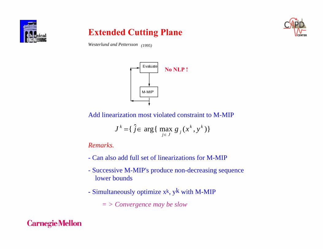
Extended Cutting Plane Westerlund and Pettersson (1992)

M-MIP'

Evaluate

Add linearization most violated constraint to M-MIP

Jk = j j∈ arg max

j∈Jg j(x k , y k )

Remarks.

- Can also add full set of linearizations for M-MIP

- Successive M-MIP's produce non-decreasing sequence lower bounds

- Simultaneously optimize xk, yk with M-MIP

= > Convergence may be slow

),(maxargˆ kkjJj

k yxgjJ∈

∈=

No NLP !

(1995)

LP/NLP Based Branch and Bound Quesada and Grossmann (1992)

Integrate NLP and M-MIP problems

NLP2M-MIP

M-MIP

LP1

LP2LP3

LP4 LP5 = > Integer

Solve NLP and update bounds open nodes

Remark.

Fewer number branch and bound nodes for LP subproblems

May increase number of NLP subproblems

(Branch & Cut)

Numerical Example

min Z = y1 + 1.5y2 + 0.5y3 + x12 + x22 s.t. (x1 - 2) 2 - x2 < 0 x1 - 2y 1 > 0 x1 - x2 - 4(1-y2) < 0 x1 - (1 - y1) > 0 x2 - y2 > 0 (MIP-EX) x1 + x2 > 3y3 y1 + y2 + y3 > 1 0 < x1 < 4, 0 < x2 < 4 y1, y2, y3 = 0, 1 Optimum solution: y1=0, y2 = 1, y3 = 0, x1 = 1, x2 = 1, Z = 3.5.

Starting point y1= y2 = y3 = 1.

Iterations

Objective function

Lower bound GBD

Upper bound GBD

Lower bound OA

Upper bound OA

Summary of Computational Results Method Subproblems Master problems (LP's solved) BB 5 (NLP1) OA 3 (NLP2) 3 (M-MIP) (19 LP's) GBD 4 (NLP2) 4 (M-GBD) (10 LP's) ECP - 5 (M-MIP) (18 LP's)

Example: Process Network with Fixed Charges

• Duran and Grossmann (1986)Network superstructure

1

2

6

7

4

3

5 8

x1

x4

x6

x21

x19

x13

x14

x11

x7

x8

x12

x15

x9

x16 x17

x25x18

x10

x20

x23x22 x24x5

x3x2

A

B

C

D

F

E

Example (Duran and Grossmann, 1986)

Algebraic MINLP: linear in y, convex in x

8 0-1 variables, 25 continuous, 31 constraints (5 nonlinear)

NLP MIP

Branch and Bound (F-L) 20 -

Outer-Approximation: 3 3

Generalized-Benders 10 10

Extended Cutting Plane - 15

LP/NLP based 3 7 LP's vs 13 LP's OAA

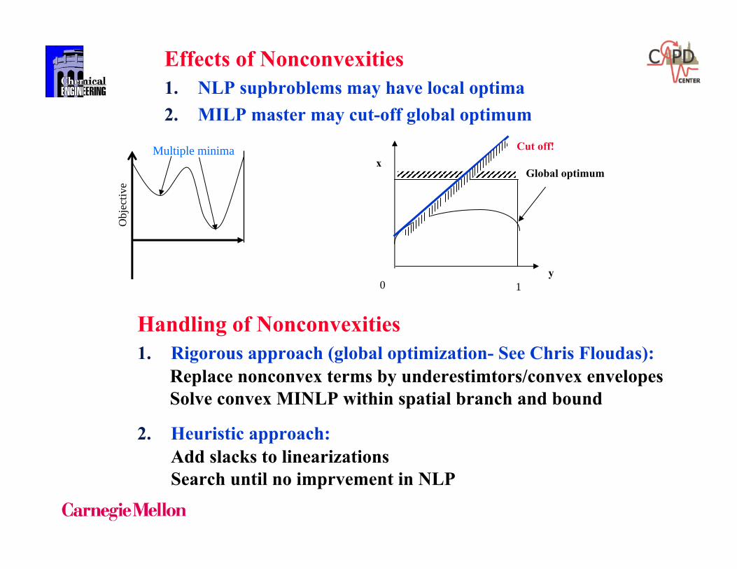
Effects of Nonconvexities1. NLP supbroblems may have local optima2. MILP master may cut-off global optimum

Obj

ectiv

e

Multiple minima

0 1y

xGlobal optimum

Cut off!

Handling of Nonconvexities1. Rigorous approach (global optimization- See Chris Floudas):

Replace nonconvex terms by underestimtors/convex envelopesSolve convex MINLP within spatial branch and bound

2. Heuristic approach:Add slacks to linearizationsSearch until no imprvement in NLP

Handling nonlinear equationsh(x,y) = 0

1. In branch and bound no special provision-simply add to NLPs

2. In GBD no special provision- cancels in Lagrangian cut

3. In OA equality relaxation

Lower bounds may not be validRigorous if eqtn relaxes as h(x,y) ≤ 0 h(x,y) is convex

[ ]1 0

, 1 0

0 0

( , ) 0

k

i

k k k k

ii ii i

k

i

kk k k T

k

if

T t t if

if

x xT h x y

y y

λ

λ

λ

>

= = − <

=

⎡ ⎤−∇ ≤⎢ ⎥

−⎣ ⎦

⎧⎪⎨⎪⎩

MIP-Master Augmented Penalty Viswanathan and Grossmann, 1990

Slacks: pk, qk with weights wk

min ZK = α + w p

k pk + wqkqkΣ

k=1

K

(M-APER)

s.t. α > f xk,yk + ∇ f xk,ykT x–xk

y–yk

T k ∇h xk,ykT x–xk

y–yk < pk

g xk,yk + ∇g xk,ykT x–xk

y–yk < qk

k=1..K

yiΣ

i ∈ Bk– yiΣ

i ∈ Nk≤ Bk – 1 k = 1,...K

x∈ X , y∈Y , α∈ R1 , pk, qk > 0

If convex MINLP then slacks take value of zero => reduces to OA/ER

Basis DICOPT (nonconvex version)

1. Solve relaxed MINLP

2. Iterate between MIP-APER and NLP subproblem until no improvement in NLP

Kk

qyyxx

yxgyxg

pyyxx

yxhT

yyxx

yxfyxfts

kk

kTkkkk

kk

kTkkk

k

kTkkkk

,...1

),(),(

),(

),(),(..

=

⎪⎪⎪⎪

⎭

⎪⎪⎪⎪

⎬

⎫

≤⎥⎥⎦

⎤

⎢⎢⎣

⎡

−

−∇+

≤⎥⎥⎦

⎤

⎢⎢⎣

⎡

−

−∇

⎥⎥⎦

⎤

⎢⎢⎣

⎡

−

−∇+≥α

MINLP: Algorithms Branch and Bound (BB) Leyffer (2001), Bussieck, Drud (2003) Generalized Benders Decomposition (GBD) Geoffrion (1972) Outer-Approximation (OA) Duran and Grossmann (1986) Extended Cutting Plane(ECP) Westerlund and Pettersson (1992) Codes: SBB GAMS simple B&B MINLP-BB (AMPL)Fletcher and Leyffer (1999)

Bonmin (COIN-OR) Bonami et al (2006) FilMINT Linderoth and Leyffer (2006)

DICOPT (GAMS) Viswanathan and Grossman (1990) AOA (AIMSS)

α−ECP Westerlund and Peterssson (1996) MINOPT Schweiger and Floudas (1998) BARON Sahinidis et al. (1998)

Mixed-integer Nonlinear Programming

IBMA.R. Conn, J. Lee, A. Lodi, A. Wächter

Carnegie Mellon University L. T. Biegler, I.E. Grossmann, C.D. Laird, N. Sawaya (Chemical Eng.)G. Cornuéjols, F. Margot (OR-Tepper)

Bonmin-An Algorithmic Framework for Convex Mixed Integer Nonlinear Programs

COIN-OR is a set of open-source codes for operations research. Contains codes for :Linear Programming (CLP)Mixed Integer Linear Programming (CBC, CLP, CGL)Non Linear Programming (IPOPT)

Software in COIN-OR

Goal: Produce new MINLP software

http://egon.cheme.cmu.edu/ibm/page.htm Pierre Bonami

BonminSingle computational framework that implements:- NLP based branch and bound (Gupta & Ravindran, 1985)- Outer-Approximation (Duran & Grossmann, 1986)- LP/NLP based branch and bound (Quesada & Grossmann, 1994)

a) Branch and bound schemeb) At each node LP or NLP subproblems can be solved

NLP solver: IPOPT MIP solver: CLPc) Various algorithms activated depending on what subproblem

is solved at given nodeI-OA Outer-approximation I-BB Branch and boundI-Hyb Hybrid LP/NLP based B&B

http://projects.coin-or.org/Bonmin

Logic-based Optimization

Motivation

1. Facilitate modeling of discrete/continuous optimization problems through use symbolic expressions

2. Reduce combinatorial search effort3. Improve handling nonlinearities

Emerging techniques1. Constraint Programming Van Hentenryck (1989)

2. Generalized Disjunctive Programming Raman and Grossmann (1994)

3. Mixed-Logic Linear Programming Hooker and Osorio (1999)

Generalized Disjunctive Programming (GDP)

( )

Ω

,0)(

0)(

)(min

1

falsetrue,YRc,Rx

trueY

K k γc

xgY

Jj

xs.t. r

xfc Z

jk

k

n

jkk

jk

jk

k

kk

∈

∈∈=

∈⎥⎥⎥

⎦

⎤

⎢⎢⎢

⎣

⎡

=

≤∈

≤

∑ +=

∨

• Raman and Grossmann (1994) (Extension Balas, 1979)

Objective Function

Common Constraints

Continuous Variables

Boolean Variables

Logic Propositions

OR operator

Disjunction

Fixed Charges

Constraints

Multiple Terms / Disjunctions

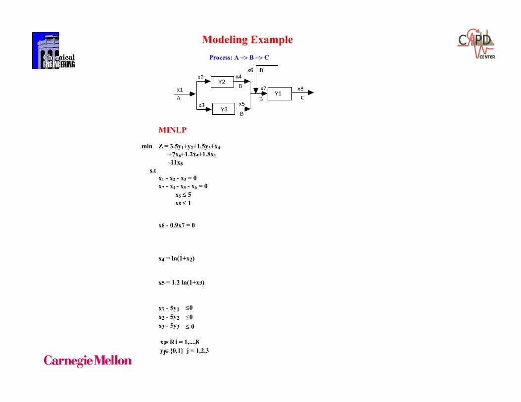
Modeling Example Process: A −> B −> C

x8x7Y1

Y2

Y3

x6x4

x5

x1

x2

x3A

B

B

B C

B

MINLP GDP

min Z = 3.5y1+y2+1.5y3+x4 min Z = c1+c2+c3+x4

+7x6+1.2x5+1.8x1 +1.8x1+1.2x5+7x6-11x8 -11x8 s.t s.t. x1 - x2 - x3 = 0 x1 - x2 - x3 = 0 x7 - x4 - x5 - x6 = 0 x7 - x4 - x5 - x6 = 0 x5 ≤ 5 x5 ≤ 5 x8 ≤ 1 x8 ≤ 1

x8 - 0.9x7 = 0

Y1x8= 0.9x7c1= 3.5

¬ Y1x7=x8=0

c1= 0∨

x4 = ln(1+x2)

Y2x4= ln (1+x2)

c2= 1

¬ Y2x2=x4=0

c2= 0∨

x5 = 1.2 ln(1+x3)

Y3x5=1.2 ln (1+x3)

c3= 1.5

¬ Y3x3=x5=0

c3= 0∨

x7 - 5y1 ? 0 x2 - 5y2 ? 0 Y2 ⇒ Y1 x3 - 5y3 ? 0 Y3 ⇒ Y1 xi∈R i = 1,...,8 xi∈R i = 1,...,8 yj∈0,1 j = 1,2,3 Yj∈True,False j = 1,2,3

≤ 0≤0≤0≤ 0

research challenges in process systems engineering and...

Documents