steady-state process optimization with guaranteed robust stability...

Lehrstuhl für Prozesstechnik Prof. Dr. Ing. W. Marquardt RWTH Aachen

Technical Report LPT-2002-01

Steady-State Process Optimization with Guaranteed Robust Stability and Feasibility

M. Moennigmann, W. Marquardt

December 2003

Published in: AIChE Journal, Vol. 49 No. 12, 2003, 3110-3126. Enquiries should be addressed to: Lehrstuhl für Prozesstechnik RWTH Aachen D-52056 Aachen Tel: +49 /(0)241 / 8094668 Fax: +49 /(0)241 / 8092326 E-Mail: [email protected]

Steady-State Process Optimization withGuaranteed Robust Stability and Feasibility

M. Monnigmann and W. Marquardt¨RWTH Aachen University, D-52056 Aachen, Germany

A new approach is presented to the optimization based design of continuous pro-cesses in the presence of parametric uncertainty. In contrast to pre®ious works focusingon process feasibility, it allows to consider both feasibility and stability of the process inthe presence of parametric uncertainty. The new approach, therefore, permits an inte-grated treatment of steady-state flexibility and robust stability in the optimization ofcontinuous processes. The process optimization problem is extended by constraints thatensure a lower bound on the distance of the nominal point of operation to stability andfeasibility boundaries in the space of the uncertain parameters. While pre®ious ap-proaches are based on e®aluating constraint ®iolation in the range space of the con-straints, the measure for flexibility and robustness used here is gi®en in the domain spaceof the uncertain parameters. The method is discussed in the context of existing ap-proaches to flexibility in process optimization and is illustrated with a continuous poly-merization which is known to ha®e a nontri®ial stability boundary resulting from multi-ple steady states and sustained oscillations.

Introduction

Models of chemical engineering processes are subject toinaccuracy and uncertainty. Numerous articles have ad-dressed the problem of process design under uncertainty over

Žthe past two decades. Grossmann and coworkers Swaney and.Grossmann 1985; Halemane and Grossmann, 1982 intro-

duced feasibility and flexibility measures on which many laterŽ .articles are based. These measures allow 1 to determine if a

given design is feasible despite the presence of parametricŽ .uncertainty, 2 to calculate a scalar index of design flexibil-

ity, which, for example, allows to compare different designs,Ž .and 3 to identify bottlenecks which impede the desired flex-

ibility. Several approaches have been suggested to solve theoptimization problems that arise in determining the proposedflexibility and feasibility measures. Early approaches had toassume that global optima occur at vertices of a hyperrectan-

Ž .gle of uncertain parameters Swaney and Grossmann, 1985 .Later research was devoted to relaxing this assumptionŽGrossmann and Floudas, 1987; Ostrovsky et al., 2000; Ka-

.batek and Swaney, 1992 . A more recent approach is based

Correspondence concerning this article should be addressed to W. Marquardt.

Žon branch and bound global optimization Floudas et al.,.2001 .

The development of process flexibility measures is still sub-Ž .ject to research. Ierapetritou 2001 presented a new ap-

Žproach to analyzing the feasible region of 1-D one-dimen-.sional quasi-convex problems, which provides a more accu-

rate description of the true feasible space than previousmethods. The approach is based on determining the convexhull of a set of points on the boundary of the feasible region.These points are determined from optimization problemssimilar to the ones proposed by Swaney and GrossmannŽ .1985 .

Based on the flexibility and feasibility measures, methodsfor process optimization under uncertainty have been devel-

Ž .oped. Bahri et al. 1996 presented a two-level optimizationprocedure for the optimization-based design of continuousprocesses in the presence of uncertainty at steady state. Theauthors evaluate design flexibility and detect critical values ofthe uncertain parameters based on constraint violation in therange space of the constraints, similar to the measures pro-

Žposed by Grossmann and coworkers Halemane and Gross-. Ž .mann, 1982; Swaney and Grossmann, 1985 . Bahri et al. 1997

December 2003 Vol. 49, No. 12 AIChE Journal3110

discuss the extension of this approach to dynamic process sys-tems.

Ž .Mohideen et al. 1996 introduce an iterative procedure foroptimization-based design in the presence of uncertainty that

Žis based on an acti®e set strategy Grossmann and Floudas,.1987 . The approach makes use of the feasibility and flexibil-

ity measures introduced by Grossmann and coworkers. Anextension of these measures to dynamic disturbances has later

Ž .been suggested Dimitriadis and Pistikopoulos, 1995 . Dy-namic disturbances are incorporated into the design processin the form of scenarios to allow for the treatment of flexibil-ity and controllability. In a successive work Mohideen et al.Ž .1997 augment their procedure by eigenvalue bounds based

Ž .on matrix measures Kokossis and Floudas, 1994 in order toavoid flexible and optimal, but unstable designs.

Ž .Bansal et al. 2001 outline a method based on parametricprogramming. This approach allows to determine explicit ex-pressions for the feasibility and flexibility measures as func-tions of the uncertain parameters a priori to the actual pro-cess design step. These explicit expressions predict in whichregions of the process parameter space feasible operation canbe guaranteed despite uncertainty. Once obtained, the ex-plicit feasibility and flexibility functions can be used to findan optimal flexible process design. This approach in particu-lar avoids two-level or nested optimizations as employed inthe methods mentioned so far. Algorithms for the solution of

Žsingle- and multiparametric MILPs Acevedo and Pistikopou-.los, 1997; Bansal et al., 2000 , and convex MINLPs where

Žuncertain parameters enter linearly Papalexandri and.Dimkou, 1998; Pertsinidis et al., 1998 and their application

to process design problems under uncertainty have been pre-sented. Both parametric programming-based design methodsand the approach presented here avoid iterations of opti-mization problems which arise because of the max-min-max

Ždefinitions of feasibility and flexibility measures Halemane.and Grossmann, 1982; Swaney and Grossmann, 1985 .

Ž .Luyben and Floudas 1994 treat controllability and eco-nomic profit as distinct objectives in a multiobjecti®e optimiza-tion approach. In this approach, open-loop controllability en-ters the optimization problem in the form of controllabilityindices for a linear approximation of the process at an oper-ating point. While not addressed by Luyben and FloudasŽ .1994 , the authors point out that flexibility and uncertaintymay be treated by considering them in additional design ob-jectives in their multiobjective optimization approach.

Much work has addressed the question of how to describeparametric uncertainty correctly and with sufficient precision.For applications in which a more precise description is tooexpensive or tedious to obtain, hyperrectangular uncertainty

Žregions are often used see, for example, Mohideen et al.,.1996, 1997; Bahri et al., 1996, 1997 . A more precise descrip-

tions can, however, be incorporated into the design proce-Ž .dures. Pistikopoulos 1995 discusses the problem of design

under stochastic uncertainty and the concept of informationcost. The impact of the precision of the description of para-metric uncertainty on the design has been investigated byRooney and Biegler who compare hyperrectangular uncer-

Žtainty regions to elliptical joint confidence regions Rooney.and Biegler, 1999 and to confidence regions derived from

Ž .the likelihood ratio test Rooney and Biegler, 2001 . Theyshow that these more precise approaches greatly improve the

description of uncertainty in the examples presented, and theyŽincorporate them into an existing algorithm Grossmann and

.Floudas, 1987 for design under uncertainty.This article addresses the steady-state optimization of con-

tinuous processes that are subject to parametric uncertainty.The major contribution of this work is a unified descriptionof the feasibility and stability boundaries, and the derivationof constraints for parametric robustness based on this de-scription. While approaches for guaranteeing feasibility in thepresence of parametric uncertainty have been established inprevious work, an equally general approach to ensuring pro-cess stability under parametric uncertainty does not exist tothe authors’ knowledge. This is the more surprising as prob-lems related to a loss of stability of optimal process designshave been encountered in applications of existing approaches

Žto optimization-based design some time ago Kokossis and.Floudas, 1994; Mohideen et al., 1997 . Roughly speaking, a

unified treatment of both feasibility and stability boundariesis possible if the notion of constraint ®iolation in the sense of

ŽGrossmann and coworkers Halemane and Grossmann, 1982;.Swaney and Grossmann, 1985 is replaced by evaluating pro-

cess designs according to their distance to critical boundariesin the space of the uncertain parameters. We call attention tothe fact that measuring constraint violation amounts to evalu-ating designs in the range space of the feasibility constraints.In contrast, the approach suggested here assesses process de-signs by measuring distances in the space of the uncertainparameters, that is, by a measure which is given directly inthe domain of the uncertain process parameters. This detail,which seems quite technical at first sight, in fact allows totreat both stability and feasibility in a unified manner.

While the examples in this article are limited to open-loopsystems, the proposed method can be applied to closed-loopsystems without modifications. This will be detailed in thenext section. For a small example of a closed-loop system, see

Ž .Monnigmann and Marquardt 2002b .¨The next section states the problem class which is ad-

dressed. It is followed by a sketch of the solution approach.This sketch introduces the notion of critical boundaries, andit explains how this idea applies both to feasibility constraintsand stability in process optimization. After having outlinedthe intuitive ideas, the section entitled Normal spaces to man-ifolds introduces the terminology which is necessary in thesubsequent section to state the constraints for parametric ro-bustness with respect to feasibility and stability. The concep-tual part of the article closes with the statement of the formalnonlinear program with constraints for robustness. Through-out the conceptual part, a simple fermenter model is used forillustrative purposes. Results of the application of the pro-posed approach to a more complex example, a polymeriza-tion reaction carried out in a continuous stirred tank reactorŽ .CSTR , are then reported in a subsequent section. Finally, asummary and a brief outlook are given.

A First Problem FormulationIn this article nonlinear dynamical systems are addressed

that can be modeled in terms of ordinary differential equa-tions and algebraic equations. We start with a general nonlin-ear systems notation. This notation allows us to point out

December 2003 Vol. 49, No. 12AIChE Journal 3111

that our approach can be applied to both open-loop andclosed-loop systems. In addition, this notation allows us tostate the requirements that must hold for an application ofour approach. Once the requirements have been stated, wewill introduce a strongly simplified notation which is naturalfor the normal vector constraints on which the presented ap-proach is based.

A broad class of nonlinear systems can be modeled byequations of the form

x d t s f d x d t , x a t ,u t ,d t ,� ,t , x d 0 s x d,Ž . Ž . Ž . Ž . Ž . Ž .˙ Ž . 0

0s f a x d t , x a t ,u t ,d t ,� ,t , 1Ž . Ž . Ž . Ž . Ž .Ž .

y t sh x d t , x a t ,u t ,d t ,� ,tŽ . Ž . Ž . Ž . Ž .Ž .

Ž dT aT .T nx nu nd n�where xs x x g� , ug� , dg� , � g� , yg� n y are state variables, inputs, disturbances, parameters, andoutputs of the system, respectively. In Eq. 1, t denotes time,

Ž dT aT .Tand f :s f , f and h are smooth functions which mapfrom some subset U ;� nx �� nu �� nd �� n� �� into � nx

and � n y, respectively. The state variables x and the corre-sponding equations have been partitioned into dynamic statevariables x d and differential equations f d, and algebraicvariables x a and equations f a.

We assert that closed-loop systems can be modeled in theŽ .form Eq. 1, if some of the inputs u t are replaced by refer-

Ž .ence signals r t . This is briefly explained. Assume first thatEq. 1 represents an open-loop system to be augmented by acontroller. The controller can be modeled as a nonlinear sys-tem itself. In order to distinguish it from the physical system,all symbols referring to the controller are marked with a hat.The inputs of the controller are partitioned into reference

Ž .signals r t , which, for example, comprise time-dependent setˆŽ .points, and all remaining inputs u tˆ

d d d a ˆ ˆ d dx t s f x t , x t ,r t ,u t ,d t ,� ,t , x 0 s x ,Ž . Ž . Ž . Ž . Ž . Ž . Ž .ˆ ˆ ˆ ˆ ˆ ˆ ˆŽ . 0

a d a ˆ ˆ0s f x t , x t ,r t ,u t ,d t ,� ,t 2Ž . Ž . Ž . Ž . Ž . Ž .ˆ ˆ ˆ ˆŽ .ˆ d a ˆ ˆy t sh x t , x t ,r t ,u t ,d t ,� ,tŽ . Ž . Ž . Ž . Ž . Ž .ˆ ˆ ˆ ˆ ˆŽ .

In the closed-loop system the outputs y of the system arefed to the controller inputs u, and the controller outputs y inˆ ˆturn are fed back to the inputs u of the nonlinear system 5.This yields

x d t s f d x d t , x a t , y t ,d t ,� ,t , x d 0 s x d,Ž . Ž . Ž . Ž . Ž . Ž .˙ ˆŽ . 0

d d d a ˆ ˆ d dx t s f x t , x t ,r t , y t ,d t ,� ,t , x 0 s x ,Ž . Ž . Ž . Ž . Ž . Ž . Ž .ˆ ˆ ˆ ˆ ˆ ˆŽ . 0

0s f a x d t , x a t , y t ,d t ,� ,tŽ . Ž . Ž . Ž .ˆŽ .a d a ˆ ˆ0s f x t , x t ,r t , y t d t ,� ,t 3Ž . Ž . Ž . Ž . Ž . Ž .ˆ ˆ ˆŽ .

0s y t yh x d t , x a t , y t ,d t ,� ,tŽ . Ž . Ž . Ž . Ž .ˆŽ .

ˆ d a ˆ ˆ0s y t yh x t , x t ,r t , y t ,d t ,� ,tŽ . Ž . Ž . Ž . Ž . Ž .ˆ ˆ ˆ ˆŽ .

System 3 is of the form of Eq. 1 without output equations,d Ž dT dT .T a Ž aT aT T T .Tif the replacements x § x , x , x § x , x , y , y ,ˆ ˆ ˆ

d dT dT T a aT aT T ˆ T T TŽ . Ž Ž . Ž . . Žf § f , f , f § f , f , yyh , yyh , d§ d ,ˆT T T ˆT T. Ž .d , � § � ,� , and u§ r are made. Note that after

closing the loop, the output equations form a system of alge-braic equations which will in general no longer explicitly yieldy and y. Thus, the closed-loop system will in general com-ˆprise algebraic equations even if the open-loop system andthe controller do not.

Since Eq. 1 can be used to model both closed-loop andopen-loop systems, we will not distinguish between the twotypes of systems further.

In order to simplify the notation we will omit the time-de-aŽ . dŽ . Ž .pendencies in x t , x t , u t and so on. Furthermore, we

will assume that the linearization of the algebraic equationsf a in Eq. 1 with respect to x a have full rank. By virtue of the

Ž .implicit function theorem IFT , the algebraic variables canthen be expressed as a function of the remaining variables.

a d a IFT a a d0s f x , x ,u ,d ,� ,t x s x x ,u ,d ,� ,t 4Ž . Ž . Ž .™

and the differential-algebraic model is of index one. Substi-Ž .tuting Eq. 4 into the nonlinear system Eq. 1 yields a simpli-

fied nonlinear system without algebraic equations

xs f x ,u ,d ,� ,t , x 0 s x 5Ž . Ž . Ž .˙ 0

ysh x ,u ,d ,� ,t ,Ž .

where the label d for the dynamic variables is omitted forŽ .simplicity. We will focus on systems of this type Eq. 5 and

defer the discussion of systems with algebraic equations tothe appendix.

Having established the terms state variables x, input andreference signals u and r, disturbances d, and parameters � ,the restrictions for an application of the approach presentedin this article can be stated. Most importantly, we will exclu-sively address the design of continuous processes operated atsteady state. These may either be open-loop or closed-loopprocesses. In detail we will assume that the following restric-tions hold:Ž .1 Equations f and h in Eq. 5 must not explicitly depend

on t.Ž . Ž .2 Inputs u t can be partitioned into a constant mean

value and bounded time-dependent variations

lower upperu t su q� t , � F� t F� � t 6Ž . Ž . Ž . Ž .i i u u u ui i i i

Furthermore, the variations are slow compared to the timescales of the system Eq. 5, that is

d�1 ui � �� Re � , � i , j, 7Ž .Ž .j� dtui

Ž .where Re � denote the real parts of the eigenvalues � ofj jthe Jacobian of f with respect to x, evaluated at the steadystate of interest.


Ž . Ž . Ž .3 The assumptions on u t must also hold for d t .Ž . Ž .4 In the closed-loop case, the assumptions on u t must

Ž .also hold for r t .These assumptions allow us to simplify the notation fur-

ther. Equations 6 and 7 imply that inputs u, references r,and disturbances d vary only quasistatically compared to thesystem dynamics, and, thus, can be modeled in terms of amean value and a parametric uncertainty. Parameters � arenot time-dependent and can be modeled in the same man-ner. Note, however, that some of the parameters are typicallynot uncertain, or the uncertainty can be neglected in the givenmodel. If Eq. 5 models a tank reactor, for example, the vol-ume of the reactor may be a parameter � for which the un-icertainty can be neglected for all practical purposes. Simi-larly, there may be inputs u for which the uncertainty can beineglected.

The assumptions suggest to repartition inputs, references,disturbances, and parameters into those which are uncertainand those for which uncertainty does not exist or can be ne-glected. We will, therefore, rewrite the ordinary differential

Ž .equations of the system Eq. 5 as

xs f x ,� , p , x 0 s x , 8Ž . Ž . Ž .˙ 0

ysh x ,� , pŽ .

where � denotes those inputs u, references r, disturbancesd, and parameters � that are modeled in terms of an averagevalue and an uncertainty, while p denotes all inputs, refer-ences, disturbances, and parameters for which uncertainty canbe neglected. For the lack of a better term, � and p will bereferred to as uncertain parameters, and parameters whichare not subject to uncertainty, respectively. The output equa-tion does not impact our results, since the outputs y do notenter the state equations. The output equations are, there-fore, omitted subsequently.

Nontrivial process optimization problems for systems of thetype of Eq. 8 at steady state involve inequality constraintsthat account for, for example, product quality or safety re-strictions. Let � and � in Figure 1 represent uncertain1 2process parameters, and let M c represent a boundary givenby such a constraint. Clearly, in process optimization thenominal point of operation � Ž0. is required to stay outside ofthe region bounded by M c. One approach to process flexibil-ity is to ensure that the constraint which corresponds to M c

not only holds for the nominal point, but for all points insome ®icinity of the nominal point. Let the region bounded byM r in Figure 1 represent this vicinity of � Ž0.. The size andshape of this region reflects the desired flexibility. If, for agiven design, the regions bounded by M c and M r in Figure 1have an empty intersection, the design will be flexible in thesense that process operation will remain feasible even in thepresence of the uncertainty described by M r. It will be shownthat stability can be described in terms of a boundary likeM c; thus, the same line of thoughts applies to stability bound-aries. Note that Figure 1 is incomplete in that more than oneboundary M c may be present, for example, because both a

Figure 1. Abstract parametric flexibility problem.

feasibility and a stability boundary have to be taken into ac-count. For simplicity of presentation, we assume first that onlyone such boundary exists. Multiple constraints are treatedfurther below.

Denoting the regions bounded by M c and M r by Rc andRr, respectively, we can state the process optimization prob-lem with flexibility and parametrically robust stability

min � x Ž0. ,� Ž0. , pŽ0. aŽ .Ž .Ž0. Ž0. Ž0.x , � , p

Ž0. Ž0. Ž0.s.t. 0s f x ,� , p aŽ .Ž . 9Ž .r Ž0. Ž0. c Ž0.0u sR � , p � R p cŽ .Ž . Ž .

Ž0. Ž0. Ž0.x g X , � g A , p gP . dŽ .

As introduced before, x g � nx are state variables, � g � n�

are uncertain parameters, p g � np are parameters whichare not affected by uncertainty, and X ;� nx, A;Rn�, P;� np represent simple box constraints on the respective vari-ables and parameters. The upper index zero denotes thenominal point of operation. In particular � Ž0. are the nomi-nal values of the uncertain parameters. Equation 9b guaran-tees that the optimal point of operation is a steady state ofEq. 8. Equation 9c guarantees that the regions bounded byM c and M r have an empty intersection and, therefore, M c isnot crossed for any value � g Rr. We allow Rr to vary inshape and size when the nominal point � Ž0. is varied. Simi-larly, both Rr and Rc may depend on p. We will write

rŽ . cŽ . rŽ . cŽ .R � , p , R p and, accordingly, M � , p , M p to pointout these dependences where appropriate.

Unified Treatment of Stability and FeasibilityŽ .The problem statement Eq. 9 is preliminary. Obviously,

the constraint in Eq. 9c needs further discussion. We willproceed by explaining first how Eq. 9c can be stated for feasi-bility constraints based on maximizing the constraint viola-tion. After pointing out the difference between feasibilityconstraints and stability constraints, we show that both canbe treated in a unified manner if the notion of the constraint


violation is replaced by the notion of the closest critical pointsin the space of uncertain parameters.

Assume that a feasibility constraint

0F g x ,� , p 10Ž . Ž .

Žwhere g maps into �, has to be enforced for the system Eq.. c8 of interest. The corresponding boundary M is given by

M cs �g A , xg X , pgP : 0s g x ,� , p , 0s f x ,� , p� 4Ž . Ž .11Ž .

For a constraint of this type, Eq. 9c can be recast in the form

0F g x ,� , p for all �gM r. 12Ž . Ž .

Existing approaches to process design under uncertainty arebased on finding an appropriate sample of values of � whichreplaces Eq. 12. Such a sample can be identified by maximiz-ing the constraint violation, that is, maximizing g over allsteady states �gM r for a fixed p. These approaches arebased on the assumption that maxima of g correspond to‘‘worst points’’ in the sense that they violate Eq. 12 with ex-

Žtremal values on the righthand side Swaney and Grossmann,.1985; Halemane and Grossmann, 1982 .

Unfortunately, for stability boundaries a simple conditionlike Eq. 12 does not exist. The stability of a given steady statecould be tested for by calculating the eigenvalues of the lin-earized process model at a steady-state operating point ofinterest. If all eigenvalues are in the open left half of thecomplex plane, the nonlinear process is locally exponentially

Ž .stable Hahn, 1967 , while the existence of one or moreeigenvalues in the open right half of the complex plane im-plies instability. A calculation of the eigenvalues is tedious,however, in particular if it has to be repeated for a sample ofpoints � which represents Eq. 12. Similarly, identifying theworst points by maximizing real parts of the eigenvalues would

Ž .be computationally demanding. Kokossis and Floudas 1994Ž .and Mohideen et al. 1997 avoided the tedious calculation of

all eigenvalues by using matrix measures. Matrix measurescan provide a single upper bound for all eigenvalues. Thisbound should, however, not be used, because it is typicallynot tight and, therefore, may result in an overestimation ofthe stability boundary at the price of obtaining a suboptimalprocess design only.

Ž .While a simple inequality Eq. 12 does not exist for stabil-ity boundaries, a meaningful definition of M c does exist. Thestability boundary is characterized by a real eigenvalue or acomplex conjugate pair to move from the left half complexplane onto the imaginary axis. However, instead of directlyevaluating the eigenvalue criterion, a system of equations im-plicitly defining M c can be derived based on bifurcation the-

Ž .ory Dobson, 1993 . The technical details of this descriptionwill be explained in the section entitled Stability manifold nor-mal ®ectors. At this point, it is sufficient to note that these

Ž .equations are of the form 0s g x,� , p and, therefore, the

stability boundary can be described by Eq. 11, that is, in thesame manner as a feasibility boundary.

Having obtained a description of the stability boundary, westill need to identify a measure for the parametric robustnessof a given steady state with respect to a loss of stability. Forthis purpose, we determine the parametric distance betweenthe manifolds M r and M c. In Figure 1, the closest distance �between M c and M r can be obtained from

� 2s min nTnc r� ,�

s.t. � cgM c

� rgM r 13Ž .

where n is defined as

ns� cy� r 14Ž .

Intuitively, one would like to restate the constraint Rr � Rc

s0u in Eq. 9 by the requirement that the minimal distancebetween M r and M c is greater than or equal to zero. Obvi-ously, � as defined in Eq. 13 cannot be used for stating thisrequirement, as � G0 by definition. The points marked bydots in Figures 2a and 2b, for example, yield �s0, and,therefore, Eq. 13 does not allow to distinguish betweenRr � Rcs0u in Figure 2a and Rr � Rc�0u in Figure 2b.

Ž .We emphasize that the vector Eq. 14 is a normal ®ectorboth with respect to manifolds M c and M r in Figure 2a. Inthe section entitled Relation to minimization of parametric dis-tance, we discuss how Eq. 13 relates to normal vectors on M r

and M c, and how normal vectors can be used to replace theconstraint Rr � Rcs0u in Eq. 9. This can, in fact, be done ina way which retains the intuitive idea of the distance betweenM r and M c of Eq. 13, while avoiding the problem of notbeing able to distinguish the cases shown in Figure 2.

Normal Spaces to ManifoldsIn this section we briefly introduce the notion of a mani-

fold and its tangent and normal space. A basic understandingand a more precise terminology than used before are prereq-uisites for stating the constraints for robust stability and ro-bust feasibility in the next section.

A nonempty set M;� n is called a smooth manifold ofdimension nyk, k� n, if, for all points agM, there exists

Ž . nan open neighborhood U a ;� and k smooth functions

� : U a ™�, . . . , � : U a ™� 15Ž . Ž . Ž .1 k

such that the Jacobian of � with respect to � has full rankŽ .for all � gU a and

M �U a s � gU a : � � s0 16� 4Ž . Ž . Ž . Ž .

Ž n.For basic notions of differential geometry in � see, forŽ .example, Fleming 1977 . For our purposes, it is often suffi-


Figure 2. Robustness manifold and critical manifold( ) ( )touch a and intersect b .

Ž .The dashed line in a marks the common normal directionat the point of intersection of M r and M c. At the points inŽ .b no such common normal direction exists.

cient and more convenient to describe the manifold in termsof the functions that generate it in � n. Thus, we let k given

Ž . Ž .smooth functions Eq. 15 define an ny k -dimensionalmanifold. This simplifies Eq. 16, since the manifold no longerhas to be given in terms of generally different functions on a

Ž .patchwork of neighborhoods U a . Equation 16 can be re-placed by

Ms � gU :� � s0 17� 4Ž . Ž .

where U ;� n no longer depends on the point agM, but isvalid for all points on the manifold. Note that M c, as definedin Eq. 11, is of the form of Eq. 17.

Figure 3 illustrates the dimensions n and k involved in thedefinition. It is instructive to think of a body to move alongthe manifolds M in Figure 3. Figure 3a is a sketch in �2, thatis, ns2, with two independent directions to move in. Forclarity, let these directions be fixed by two linearly indepen-dent unit vectors e and e . If we restrict motion by one1 2equation, that is, ks1, this equation will, roughly speaking,fix steps along the unit vector e for a given step along e2 1and vice versa, confining motion to a one-parametric curve,

Ž . 3that is, a 1-D manifold nyks1 . Similarly, in � spanned

Figure 3. Normal and tangent space for a curve in lR2

and a surface in lR3.

by appropriate vectors e , e , e , a single equation will fix the1 2 3step along one of the unit vectors for given steps along theother two unit vectors, confining motion to a 2-D surface,

Ž .that is, a 2-D manifold nyks2 . Thinking in terms of con-straints in optimization again, the 1-D manifold in the �2

example splits the �2 into those parts in which the constraintis violated and those parts in which it is inactive. Similarly,the 2-D manifold in the �3 example splits the �3 into twosuch parts.

A basic result from differential geometry states that a lin-ear subspace, the tangent space, can be attached to any pointon the manifold locally. As pointed out in the examples aboveand as expected intuitively, the k equations defining themanifold fix k of the degrees of freedom in � n, leaving nyklinearly independent directions to move locally tangentially

Ž .to the manifold. These directions span the ny k -dimensional tangent space at a given point on the manifold.Again, as expected intuitively, there exist k independent di-rections in � n which are normal to the nyk directions thatspan the tangent space. Orthogonality is with respect to theusual inner product. Note that tangent and normal spaces areunique, while the directions which span them in general arenot.

In the examples given above, the tangent space to the curve2 Ž 2.in � that is, to the 1-D manifold in � is 1-D. The normal


space is the 1-D straight line orthogonal to the curve at therespective point. The tangent space of the 2-D surface in �3

Ž 3.that is, the 2-D manifold in � is the 2-D plane tangent tothe manifold at the point of interest, while the normal spaceis the straight line normal to the manifold through this point.See Figures 3a and 3b for a sketch.

The notion of a manifold allows us to carry over the con-cept of a normal space, which we intuitively use in �2 and �3

correctly, to higher dimensional spaces. More precisely, let-Ž .ting the k functions in Eq. 15 define an nyk -dimensional

manifold in � n, the k vectors in � n

b s� , . . . , b s� 18Ž .1 1 k k

evaluated at a point on the manifold of interest are linearlyindependent and span the normal space to the manifold at

Ž . Ž .this point Fleming, 1977 . This normal space basis Eq. 18will be illustrated with simple examples in the next section.

Flexibility and Robust Stability ConstraintsBased on the notions manifold and normal space, con-

straints can now be stated which allow to recast the require-r c Ž .ment R � R s0u Eq. 9b into a form that can be imple-

mented. Two details complicate the application of the termsintroduced in the previous section. One complication arisesbecause the equations defining the manifolds M c and M r

involve other variables than uncertain parameters � , namelythe state variables x and parameters p. Roughly speaking,we are interested in the normal vector in the subspace of theuncertain parameters � , since a measure of the distance be-tween M c and M r is needed in this subspace.

The second complication arises because a single feasibilityconstraint can not always be stated as a single inequality, butan inequality along with an equation or even a set of equa-tions are necessary. A simple example will be given below.Similarly, a constraint for stability cannot be stated as a sin-gle equation, but it involves auxiliary equations that deter-mine variables such as eigenvalues or eigenvectors which oc-cur only in the stability constraint, but not in the model or inother constraints. Note that this complication does not resultfrom multiple constraints, but from a single constraint whichcannot be stated as a single equation or inequality. Multipleconstraints will be treated in the section entitled Optimizationwith flexibility and robust stability constraints.

The present section resolves these complications. For illus-trative purposes, a simple model of a continuous fermenta-tion process is introduced.

Illustrati©e fermentation process exampleA simple model for a fermentation process in a CSTR is

given by

FXsy Xq S X s f 19Ž . Ž .1V

FSs S yS y� S Xs fŽ .Ž .F 2V

w y3 x w y3 xwhere X kg m and S kmol m are the cell concentra-w y1 x wtion and the substrate concentration, F kg s , S kmolF

y3 x w 3xm , and V m denote the feed, substrate concentration inŽ . Ž .the feed and the reactor volume, and S skS exp ySrK

w y1 x Ž . Ž . Ž . w y1 y1 xs and � S s S r aqbS kg kmol s are thegrowth and substrate consumption rate, respectively. In the

3 Ž . y1calculations to follow, we set ks1 m kmol s , Ks0.12kmol m3, �s5.4 kg kmoly1, bs180 kg m3 kmoly2, Vs�Ž .23m 5.7 m. For details on the process model, we refer to

Ž .Brengel and Seider 1992 .y1Ž .F is replaced by FsFr 10 kg s for better numerical

scaling. We assume that S and F are subject to uncertainty,FT TŽ . Ž .that is, �s F, S , furthermore xs X, S . The parame-F

Ž .Tters ps k, K , a, b, V are assumed to be known preciselyin this simple example.

Feasibility boundary normal ©ectorsFor simplicity, it has so far been assumed that a feasibility

constraint is given by a single inequality

0F g x ,� , p , 20Ž . Ž .

where g maps into �. The corresponding feasibility boundaryc ŽM is defined by the steady states of the process model Eq.

.8 at which this constraint is active

M cs x ,� , p gU : 0s g x ,� , p , 0s f x ,� , p . 21� 4Ž . Ž . Ž . Ž .

U ; � nx � � n� � � np is an appropriate domain for thevariables which depends on the process of interest. A largerclass of constraints can be accounted for, if we allow the scalarfunction g to be replaced by a vector-valued function. Thistype of constraint arises if g depends on intermediate or aux-iliary variables x, which are not part of the process model,˜but nevertheless have to be introduced to state the con-straint. We first discuss the general form of constraints ofthis type and give a brief example below. The general formreads

0s g x , x ,� , p aŽ . Ž .ˆ ˜22Ž .

0F g x , x ,� , p bŽ . Ž .˜

˜ nxwhere g and g are smooth, defined on some subset U ;�ˆnx n� np nx�� , and map into � and �, respectively. The

nxauxiliary variables are denoted by xg � . Furthermore, the˜Jacobian of g with respect to x is assumed to have full rank.ˆ ˜This property will be used below to guarantee that Eq. 22acan be solved for x locally.˜

The feasibility boundary M c that corresponds to Eq. 22 isŽ .defined by the steady states of the process model Eq. 8 at

Ž .which Eq. 22a holds, and at which the inequality Eq. 22b isactive. Using the abbreviation

g x , x , � , p :s g x , x , � , p , . . . , 23Ž . Ž . Ž .˜ ˜ ˆ ˜Ž 1

Tg x , x , � , p , g x , x , � , pŽ . Ž .ˆ ˜ ˜ .nx


Ž . cthe definition Eq. 21 of M therefore generalizes to

c ˜M s x , x , � , p gU : 0s g x , x , � , p , 0s f x , � , p .Ž . Ž . Ž .˜ ˜ ˜� 424Ž .

Ž .TIt is stressed that gs g , . . . , g , g comprises n q1˜ ˆ ˆ1 n xx

equations, whereas x has only n entries. While counter-in-˜ xtuitive at first sight, this can be clarified by counting dimen-

Žsions. Loosely speaking, the n q1 equations 0s g x, x, � ,˜ ˜x.p in Eq. 24 fix the n auxiliary variables as well as one of thex

variables x of the model. It is instructive to see that this alsoiŽ .holds for the case of a single inequality Eq. 20 , and that this

Ž .case is recovered from the general formulation Eq. 22 bysetting n s0. In this case, no auxiliary Eq. 22a nor auxiliaryxvariables x exist, and Eq. 22 is reduced to the single inequal-˜

Ž . Žity Eq. 22b . Likewise, the set of n equations 0s g x, x, � ,˜ ˜x. Ž .p in Eq. 24 is reduced to the single equation 0s g x, � , p

in Eq. 21. This single equation obviously does not determineany auxiliary variables, but it still fixes one of the variables xi

Ž .of the model that is, n q1s1 .xŽ .Constraints of the type Eq. 22 arise, for example, if an

inequality constraint is a function of outputs y of the processŽ .model Eq. 8 . A constraint of the type

ysh x , � , pŽ .25Ž .

0F g x , y , � , pŽ .

Ž .can be rewritten in the form Eq. 22 using x:s y and˜Ž . Ž .g x, x, � , p :s xyh x, � , p . While Eq. 25 provides explicitˆ ˜ ˜

Žformulas for the auxiliary variables xs y, the constraint Eq.˜.22 is more general in that one may not be able to solve Eq.

22a for the x explicitly. By assumption, Eqs. 22a have full˜rank with respect to x, however. The implicit function theo-˜rem, therefore, implies that Eqs. 22 can be solved for the xlocally.

Having stated the general form of feasibility constraintsŽ . Ž .Eqs. 22 and the corresponding definition Eq. 24 of thecritical manifold M c, normal vectors to M c can be intro-

Ž T T .T Ž T T .Tduced. We use s x , x and �s f , g as abbrevia-˜ ˜tions. According to Eq. 18, the normal space to the manifoldŽ .Eq. 24 is spanned by

� � n qn q1 1 x xb s , . . . , b s 26Ž .1 n qn q1x x �ž /�� ž /� n qn q11 x x

evaluated at the point on the manifold of interest. Since welook for the normal vector in the space of the uncertain pa-rameters � , we seek a linear combination in the normal spacethat does not have a contribution along the variables u. Such

nxqn xq1 Ž .a linear combination kg� of the vectors Eq. 26can be determined from

� � � . . . � ks0 aŽ .Ž . 1 n qn q1x x 27Ž .Tk ky1s0, bŽ .0

where the second equation for some k not normal to k0guarantees that the trivial solution ks0 is rejected. The pa-rameter space normal vector n can be evaluated from the

Ž .remaining rows of the basis vectors Eq. 26

ns �� . . . � k . 28Ž .Ž .1 � n qn q1x x

Ž .Monnigmann and Marquardt 2002a show that Eqs. 27 and¨28 yield a unique normal direction.

As an illustration, we assume that the constraint

0F0.7 kmol my3yS s: g S 29Ž .Ž .F F

applies in the fermenter example. Since n s0, we have sxŽ .T Ž T T .Txs X,S and �s f , g where f refers to Eq. 19. Equa-

tion 27a evaluates to

Fky F q S y� S 0Ž . Ž . 10V 0k s2 ž /0F � 0� � k� 0 3 S X y F y� S X 0Ž . Ž .0V

30Ž .

Ž .Twhich is solved by ks 0, 0, 1 . This solution is unique apartfrom a nonzero scaling factor. It obeys Eq. 27b for the choicek sk. Evaluating Eq. 28 yields the normal vector0

F X F S ySŽ .0 0 F ky 0 1V V 0kns s 31Ž .2 ž /y1FF0 � 0k� 0 30 y1

V

Due to the simplicity of Eq. 29, the normal vector is indepen-dent of � . This result is visualized in Figure 4 along with less

Figure 4. Examples of normal vectors for the fermenter.c,1 Ž . c,2M corresponds to the feasibility constraint Eq. 29 . M

and M c,3 correspond to stability boundaries due to Hopf andsaddle-node bifurcations. Figures 5a and 6a are obtained byplotting X along the dashed lines at S s 0.3 kmol my3 andFS s 0.2 kmol my3, respectively.F


trivial examples of normal vectors to be explained in the nextsection.

Stability manifold normal ©ectorsStability manifold normal vectors will be introduced for

process models which consist of ordinary differential equa-Ž .tions ODE only

xs f x , � , p 32Ž . Ž .˙

The extension to models with algebraic equations is deferredŽ .to the appendix. The ODE model Eq. 19 of the fermenter

will be used in subsequent illustrations.The aim of the present section is to describe the loss of

stability of an ODE process model by a set of algebraic con-straints, which will allow for a characterization of stability

Ž .boundaries in terms of manifolds of the form Eq. 17 . Notethat stability is a property of the dynamical system modeledby differential equations. It is therefore not trivial that a de-scription of stability in terms of algebraic equations exists atall. As explained briefly in the section entitled Solution ap-proach, such an algebraic description is possible based on theobservation that the existence of an eigenvalue on the imagi-nary axis is a necessary condition for a loss of stability. Be-

Figure 5. Equilibria of the fermenter for S s0.3 kmolF�3 ( )m a and behavior of eigenvalues in the

( )vicinity of the stability boundary b .

fore proceeding to the normal vector systems, this is illus-Ž .trated further with the fermentation process example Eq. 19 .

Figure 5a shows values of the cell concentration X forequilibria over a range of the dimensionless feed F and afixed value S s0.3 kmol my3. The eigenvalues of the lin-Fearized process model evaluated along the points shown inthe enlargement are depicted in Figure 5b. The loss of stabil-ity occurs when the complex conjugate pair of eigenvaluescrosses the imaginary axis. Figures 6a and 6b show similarplots for a fixed substrate feed concentration S s0.2 kmolFmy3. In this case, the process loses stability as a single realeigenvalue crosses the imaginary axis. The second real eigen-value is not shown in Figure 6b, since it is well below zeroand, therefore, its influence on stability can be neglected.

The illustrated examples correspond to the simplest twocases by which a loss of stability can occur, that is, a singlereal eigenvalue or a pair of complex conjugate eigenvaluesmoving from the left half into the right half of the complexplane. The remainder of this section will state the systems ofequations which correspond to the existence of a real eigen-value and a complex conjugate pair on the imaginary axis.

Before proceeding to these systems, we stress that a loss ofstability need not occur due to exactly one real eigenvalue orexactly two complex conjugate eigenvalues on the imaginaryaxis, but may involve any combination of these two basic cases

Figure 6. Equilibria of the fermenter for S s0.2 kmolF�3 ( )m a and behavior of eigenvalues in the

( )vicinity of the stability boundary b .


leading to a larger number of eigenvalues on the imaginaryaxis. For a point to lie on the stability boundary, however, atleast a real eigenvalue or a complex conjugate pair of eigen-values must exist on the imaginary axis. Thus, the systems ofequations presented below are necessary conditions for a lossof stability. In fact it is known from bifurcation theory that aloss of stability typically occurs due to either exactly one sin-gle real, or exactly one complex conjugate pair of eigenvalueson the imaginary axis, and that more complicated situationsinvolving combinations of the two cases rarely occur in physi-cal systems. More precisely, bifurcation theory states that in an -dimensional parameter space, the stability boundary will�

Ž .be given by n y1 -D manifolds of equilibria with either a�

single real or a complex conjugate pair on the imaginary axis,while combinations of the two basic cases will occur only in

Ž .the manifolds or, more generally, sets of dimensions of atmost n y2. A thorough discussion of this issue is beyond�

the scope of this article. For this article, it is important tonote that both the detection of stability boundaries and thecalculation of normal vectors can be based on the necessaryconditions of a single real or a complex conjugate pair ofeigenvalues on the imaginary axis presented below. We referto summarizing articles and textbooks in the bifurcation the-

Žory Guckenheimer and Holmes, 1993; Kuznetsov, 1999; Beyn.et al., 2003 , and articles which discuss technical details of

Žnormal vectors on manifolds of bifurcation points Dobson,.1993; Monnigmann and Marquardt, 2002a .¨

At an equilibrium for which a real eigenvalue on the imagi-nary axis exists, the system of 2n q1 equationsx

0s f 33Ž .0s f T®x g5T0s® ®y1

holds. Here f T denotes the transposed Jacobian of the pro-xŽ . nxcess model Eq. 32 with respect to x, and ®g� is the

eigenvector corresponding to the eigenvalue zero. Argumentsof f and its derivatives are omitted here and in the sequel forbrevity. Equations 33 are necessary conditions for a saddle-

Ž .node bifurcation Beyn et al., 2003; Kuznetsov, 1999 . A 1-Dmanifold of points which satisfy Eqs. 33 for the fermentermodel is given by M c,3 in Figure 4.

If a complex conjugate pair of eigenvalues with real partzero exists, the system of 3n q2 equationsx

0s fŽ1. Ž2.¶0s f w q� wx

Ž2. Ž1.0s f w y� w •x g 34Ž .˜T0sw wy1 ßŽ1.T Ž2.0sw w

holds. Again, f denotes the Jacobian, wswŽ1.q iwŽ2., wgx� nx is the eigenvector of f corresponding to the eigenvaluex�s i�, �g�, and w denotes the complex conjugate of w.Equations 34 are necessary conditions for a Hopf bifurcationŽ .Beyn et al., 2003; Kuznetsov, 1999 . In Figure 4 the 1-Dmanifold M c,2 is composed of points which satisfy Eq. 34.

Equations 33 and 34 are the systems of algebraic equationsnecessary to state defining equations for the manifolds atwhich a loss of stability occurs. Substituting Eqs. 33 or 34 intoEq. 24, repeated here for convenience

c ˜M s x , x ,� , p gU : 0s g x , x , � , p , 0s f x , � , pŽ . Ž . Ž .˜ ˜ ˜� 4provides a description of the stability manifold which has thesame form as the feasibility manifolds in the previous section.Having obtained an algebraic description of the stabilityboundary, the corresponding normal vector systems can bederived by the line of arguments in Eqs. 26�28. The applica-tion of Eqs. 26�28 requires straightforward but tedious linearalgebra, thus, we only summarize the resulting normal vector

Ž .systems and refer to Monnigmann and Marquardt 2002a for¨details.

Using the notation introduced in the previous section, wehave xs® for stability boundaries due to a saddle-node bi-˜

Žfurcation. In Eqs. 27 and 28, k can be chosen to be ks ® ,1.T 2 n xq1 Ž. . . , ® , 0, . . . , 0 g� Monnigmann and Marquardt,¨n

.2002a . The n q1 trailing zeroes in k allow to reduce thexŽsize of the normal vector system considerably Monnigmann¨

.and Marquardt, 2002a . The resulting system for the normalvector n is given by the 2n qn q1 equationsx �

Equations 3335Ž .Tf ®yns0�

For stability boundaries due to a Hopf bifurcation, we haveŽ Ž1. Ž1. Ž2. Ž2. .T 2 n xq1xs w , . . . , w , w , . . . , w , � g� . Applying Eqs.˜ 1 n 1 nx x

Ž Ž1. Ž1. Ž2. Ž2. .T26�28 yields ks u , . . . , u , ® , . . . , ® , ® , . . . , ® , 0 g1 n 1 n 1 nx x

�3n xq2 and the normal vector system

Equations 34

f T®Ž1.y� ®Ž2.q� wŽ1.y� wŽ2.s0x 1 2

f T®Ž2.q� ®Ž1.q� wŽ1.q� wŽ2.s0x 1 2

®Ž1.T wŽ1.q®Ž2.T wŽ2.y1s0 36Ž .®Ž1.T wŽ2.y®Ž2.T wŽ1.s0

f Tuq®Ž1.T f wŽ1.q®Ž2.T f wŽ2.s0x x x x x

f Tuq®Ž1.T f wŽ1.q®Ž2.T f wŽ2.yns0� x � x �

which consists of 6n q2n q4 equations. The term ®Ž1. f wŽ1.x � x x

Ž Ž1. w Ž1. . Ž1.is short for the tensor product ® f s ®Ýx x i �� j�

� 2 fsŽ1.w . The other tensor products in Eqs. 36 are de-�� x � x� i

fined accordingly. Note that ®s®Ž1.q i®Ž2. g � nx can be in-terpreted as the eigenvector of f T corresponding to thexeigenvalue �sy i�. The variables � , � are auxiliary vari-1 2ables which can be shown to be always zero. They are added

Žto render the normal vector system regular Monnigmann and¨.Marquardt, 2002a .

Equations 36 contain second derivatives of f. AdiforŽ . Ž .Bischof et al., 1996 and maple Monagan et al., 2000 areused to calculate these derivatives by automatic and symbolicdifferentiation in our implementation of the method.

As an illustration, the stability boundary normal vector sys-Ž .tems Eqs. 33 and 35 are evaluated for the fermenter. The


y3 y3values Xs2.16 kg m , Ss0.120 kmol m , Fs0.712, SFs0.2 kmol my3 correspond to the equilibrium at which sta-bility is lost in Figure 6. At this point, the Jacobian has aneigenvalue of zero corresponding to the left eigenvector ®sŽ .Ty1,0 , which satisfies Eq. 33. Equation 35 evaluates to

F X F S ySŽ .0 0 FyV V y1 yns0 37Ž .ž /0FF0� 00

V

Ž .Twhich yields ns y0.0134, . The normal direction definedby this vector is shown in Figure 4.

Normal ©ectors to M r

From a technical point of view, normal vectors to the ro-bustness manifold M r can be calculated in the same manneras normal vectors to feasibility and stability boundaries. M r

differs from feasibility and stability boundaries M c in thatM r generally varies in form and shape when the nominal pointof operation is varied. As explained above, M r is allowed to

Ž0. Žvary in shape and location if � is varied see Figure 1 for.an illustration . To account for this variation, the defining

equations of M r may depend on the value of the uncertainparameters at the point of operation � Ž0.. Technically, M r isparameterized by � Ž0.; thus, � Ž0. belongs to the parametersp of the defining equations of M r. The general definition ofa manifold M r here is of the form of Eq. 24, repeated herefor convenience

r ˜M s x , x ,� , p gU : 0s g x , x , � , p , 0s f x ,� , pŽ . Ž . Ž .˜ ˜ ˜� 438Ž .

nxq1 n x˜where the smooth functions g map into � , and U ;�˜nx n� np�� .

Figure 4 illustrates normal vectors on M r. We assume thatthe parametric uncertainty of F and S in the fermenter ex-Fample can be described by the circle

2 2Ž0. Ž0.FyF S ySF FŽ0. Ž0.g F ,S ; F ,S s q y2, 39Ž .˜Ž .F F ž / ž /�S� F F

y3where � Fs0.05 and �S s0.05 kmol m . Since Eq. 39Fdoes not depend on the state variables X and S of the fer-menter, the model equations f can be omitted in this case inEq. 38. Since a single defining equation for M r remains inthis simple example, the normal space is 1-D and the singlebasis vector can be obtained from Eq. 18 to be

Ž0. Ž0.FyF S ySF F Tns2 , . 40Ž .22ž /�S� F F

Note that this corresponds to evaluating Eq. 28 with ksk0s1g�. Figure 4 visualizes normal vectors on M r for thefermenter example. The direction given by n from Eq. 40 canbe interpreted as the direction that is spanned by the line

Ž0. Ž0.Ž .drawn from the center F , S of the circle to any pointFŽ .F,S on the circle.F

Optimization with Flexibility and Robust StabilityConstraints

Having introduced the systems of equations that allow tocalculate normal vectors on manifolds M c and M r, the non-

Ž .linear program NLP for the steady-state optimization ofcontinuous processes in the presence of parametric uncer-tainty can be stated.

In summary, the normal vector systems are nonlinear setsof equations which depend on state variables x of the dy-

Ž .namic system of interest Eq. 8 , on auxiliary variables x such˜Žas the eigenvectors in systems for stability boundaries Eqs.

.33 and 34 , on the uncertain parameters � , on the parame-ters not subject to uncertainty p, and, in the case of M r dis-cussed in the previous section, on the nominal point of oper-ation � Ž0.. In the statement of the NLP below, we will there-fore abbreviate the normal vector systems by

Ž t . Ž0. � 4G x , x ,� , p ,n ,� s0, tg f , s , s , 41Ž .˜Ž . 1 2

where the index t denotes the type of manifold. An indexts f refers to feasibility boundaries. In this case, Eq. 41stands for the defining equations in Eq. 24 and Eqs. 27 and28. The indices ts s , s denote stability boundaries. In these1 2cases Eq. 41 abbreviates Eqs. 35 and 36, respectively. Aspointed out in the previous section, the normal vector systemfor M r, denoted by ts r, has the same form as the case ts f

GŽ r . x , x ,� , p ,n ,� Ž0. s0. 42Ž .˜Ž .

Ž .The optimization problem Eq. 9 can now be restated us-Ž .ing the normal vector systems Eqs. 41 and 42 . As opposed

to the introduction of Eq. 9, which focused on the existenceof one locally closest critical point for simplicity, more thanone locally closest critical point must be accounted for in thegeneral case. Multiple closest connections between M r andM c may arise because of multiple constraints, or because ofnonconvexity of constraints, cf. Figure 7. Let the upper index

� 4 Žc, i.ig Is 1, . . . , i enumerate critical points � and themaxcorresponding points � Ž r , i. on M r. For each ig I, the system

Figure 7. Typically more than one normal vector con-straint exists due to the nonconvexity of mani-folds M r, Mc, or because more than one fea-sibility and stability boundary exist.


of equations

0sGŽ r , i. x Ž r , i. , x Ž r , i. , � Ž r , i. , pŽ r , i. , nŽ i. , � Ž0.˜Ž .

0sGŽ t i ,i. x Žc , i. , x Žc , i. , � Žc , i. , pŽc , i. , nŽ i. , � Ž0.˜Ž .

yields the direction nŽ i. which is normal to the respectivemanifold at both � (r,i) and � Žc, i.. Along this normal direc-tion, the distance between � (r,i) and � (c,i) must be equal toor larger than zero. This is ensured by Eq. 46 and the in-

Ž .equality Eq. 47 in the NLP

min � x Ž0. ,� Ž0. , pŽ0. 43Ž .Ž .Ž0. Ž0. Ž0.x ,� , p

Ž0. Ž0. Ž0.s.t. 0s f x ,� , p , 44Ž .Ž .Ž r , i. Ž r , i. Ž r , i. Ž r , i. Ž r , i. Ž i. Ž0.0sG x , x ,� , p ,n ,�˜Ž .

45Ž .Ž t , i. Žc , i. Žc , i. Žc , i. Žc , i. Ž i. Ž0.i0sG x , x ,� , p ,n ,� ,˜Ž .

� 4t g f , s , si 1 2

Ž i. Ž i. Žc , i. Ž r , i.0s l n y � y� 46Ž . Ž .Ž i.0F l 47Ž .

ig I , xg X , �g A , pgP 48Ž .

which is a restatement of Eq. 9 that can be implemented.Note that x(r,i), x(r,i), � (r,i), p(r,i), nŽ i., x(c,i), x(c,i), � (c,i), p(c,i),˜ ˜l Ž i. are degrees of freedom in the optimization in addition tox Ž0., � Ž0., pŽ0.. We do not list these variables as arguments of43 to avoid a too tedious notation.

Ž .We will refer to the constraints Eqs. 45�48 as minimaldistance constraints for short. Note that this does not meanthat we seek a minimal distance, but the name is supposed toreflect that we ensure a distance greater than some accept-able lower bound.

Relation to minimization of parametric distanceŽ .The optimization problem Eq. 13 was used to introduce

the notion of parametric distance between candidate pointsof operation and critical points. With the help of Figure 2, we

Ž .pointed out that the simple optimization problem Eq. 13provides an incomplete characterization of the constraint Rr

lRcsø. It is instructive to see why the minimal distanceŽ .constraints Eqs. 45�48 avoid the problems of the straight-

forward measure � of the distance between the manifoldsintroduced in Eq. 13.

Ž T T .TUsing the notation and the abbreviation �s f , g in-˜troduced above, we can rewrite the optimization problem Eq.13 as

12 T� s min n n

r r c c 2x ,� , x ,�

s.t. 0s� c x c,� cŽ .

0s� r x r ,� r 49Ž . Ž .

0sny � cy� rŽ .

where a factor 1r2 has been introduced into the objective ascompared to Eq. 13 to simplify the comparison to follow. The

Ž .first-order Karush-Kuhn-Tucker KKT conditions for opti-mality are � rs0, � cs0 and

r � � r rr r � . . . � k s0Ž .x 1 x n n q1x x

c r r � � r rr ry � y� q � . . . � k s0Ž . Ž .� 1 � n qn q1x x

50Ž .

c � � c cc c � . . . � k s0Ž .x 1 x n qn q1x x

c r c � � c cc c� y� q � . . . � k s0Ž . Ž .� 1 � n qn q1x x

where k r and k c denote Lagrange multipliers, and argu-ments of � r, � c and their derivatives are omitted for brevity.Comparing the KKT conditions to the normal vector basedapproach reveals that the first and second rows of equations

Ž c r.in Eq. 50 correspond to Eqs. 27a and 28. Thus, � y� inEq. 50 is a normal vector to M r. Similarly, the third and fourth

Ž c r.rows in Eq. 50 reveal that � y� is a normal vector toM c. Note, however, that the KKT conditions permit the solu-tion

k rsk cs0, ns � cy� r s0 51Ž . Ž .

In contrast, the minimal distance constraints reject this typeof solution, since a finite length of k is enforced by Eq. 27b.Due to this difference, the minimal distance constraints allowto distinguish between the solutions shown in Figures 2a and

Ž .2b while the KKT conditions Eq. 50 do not. Solutions of theŽ .type Eq. 2a are accepted by the minimal distance con-

straints, since the points on M r and M c marked by the dothave a common normal direction. Note that a step of lengthzero, which is accepted by Eq. 47, is necessary along this di-rection to connect the points on M r and M c in Figure 2a. Incontrast, the points marked in Figure 2b do not have a com-mon normal direction. While they are solutions of the typeŽ .Eq. 51 of the KKT conditions, they are rejected by the min-imal distance constraints.

Application to a Continuous PolymerizationProcess

Ž .In this section, the NLP Eqs. 43�48 is solved for a poly-merization reaction carried out in a CSTR. Process modelsfor continuous homopolymerization have been presented, an-alyzed, and discussed in a series of articles by Ray and

Žcoworkers Schmidt and Ray, 1981; Hamer et al., 1981;.Schmidt et al., 1984; Teymour and Ray, 1989, 1992a,b . The

process treated here is the solution free radical homopoly-merization of vinyl acetate. The stability boundaries for themodel are known from a detailed analysis of its nonlinear

Ž .dynamic behavior Teymour and Ray, 1992b . Note that themodel was derived from a lab-scale reactor model which has

Ž .been validated experimentally Teymour and Ray, 1992a . AŽ .good summary of the model can be found in DeCicco 2000 .

We do not repeat the process model, which consists of fourdifferential and 15 algebraic equations, for the sake of brevity.


Optimization problemWe optimize the polymerization of vinyl acetate with re-

spect to the merit function

˜ w x� profitrtime sy® � C qm f m f m in

y® � C qsf s f s in

y I MW C qf I i in

q® � C q , 52Ž .p p p out

where ® and ® refer to the monomer and solvent volumem f sffraction in the feed, � , � and � are the density ofm f sf pmonomer in the feed, solvent in the feed, and polymer in thereactor, MW and I are the molecular weight and the molarI fconcentration of the initiator, � refers to the residence time,® denotes the volume fraction of polymer in the reactor, andpthe C refer to the cost coefficients of the respective sub-istances. The difference between input flow rate q and out-input flow rate q can be neglected. Therefore, we can opti-outmize with respect to the simplified merit function

w x� profitrtimerreactor volume s

y® � C y® � C y I MW C q® � C r� . 53Ž .Ž .m f m f m sf s f s f I i p p p

The optimization results presented below were obtained withthe relative cost coefficients C s3C , C s6C , C s20C .m s p m i p

The robustness manifold M r is chosen to be the ellipsoiddefined by

2 2Ž0. Ž0.� y� � y�1 1 2 2r Ž0.g � ,� s q y2, 54Ž . Ž .ž / ž /�� 1 2

where � s� , � s I and1 2 f

��s�� s5 min1

� I s�� s5 molrm3. 55Ž .f 2

Due to the simplicity of the chosen robustness manifold, thenormal vector can be calculated explicitly to be

TŽ0. Ž0.� y� � y�1 1 2 2ns2 , . 56Ž .2 2ž /�� 1 2

This simplifies Eq. 45 considerably.

ResultsWe will take into account robust stability and flexibility with

respect to a temperature restriction. For illustrative pur-poses, we switch on these constraints one at a time.

For reference, we solve the optimization problem at firstwithout robust stability and flexibility constraints

max � x Ž0. ,� Ž0. 57Ž . Ž .Ž0. Ž0.x ,�

s.t. 0s f x Ž0. ,� Ž0.Ž .

( )Figure 8. Optimum which results from the NLP Eq. 57 .The optimum is marked by the cross.

Ž .Twhere �s � , I . The resulting optimal point of operationfis �s0.777 min, I s23.4 molrm3, and Ts430 K. It isfmarked by a cross in Figure 8. Figure 8a shows all steadystates of the process as a function of � . Note that multiplesteady states exist for � up to about 50 min. As a rule ofthumb, we expect optimal points of operation to be locatedon the branch of stable steady states at high temperatures,since a high rate of polymer production will occur at hightemperature. In Figure 8a, the branch of interest is boundedbelow with respect to � by a loss of stability due to a saddle-node bifurcation and bounded above by a loss of stability dueto a Hopf bifurcation. Figure 8b shows the location of thestability boundaries which result from saddle-node and Hopfbifurcations as a function of � and I . The particular value offI , at which Figure 8a was obtained, is marked by the hori-fzontal dashed line in Figure 8b. Along this line, the points atwhich stability is lost in Figure 8a can be found. Figure 8reveals that the process design given by the optimal pointmarked by the cross cannot be considered robust, as it isparametrically close to a part of the stability boundary whichis due to the saddle-node bifurcations.

This result suggests to optimize the process with a minimaldistance constraint on the location of the closest saddle-node

� 4bifurcation. We, therefore, solve Eqs. 43�48 with Is 1 and


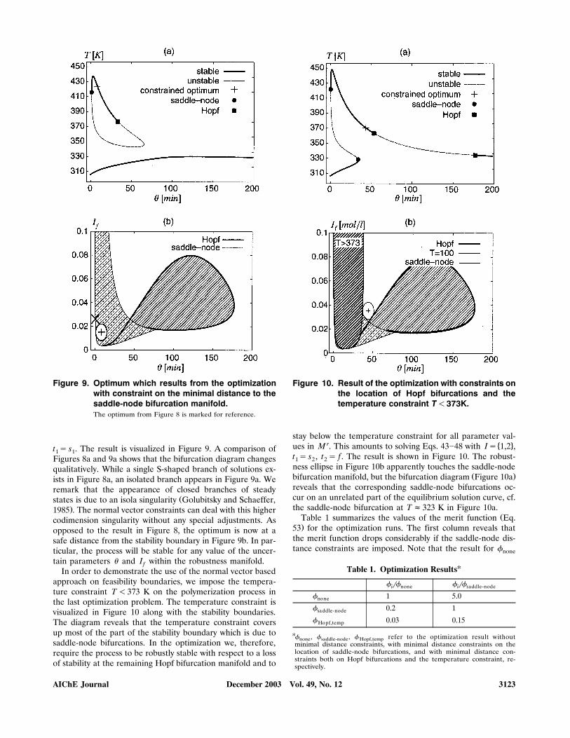
Figure 9. Optimum which results from the optimizationwith constraint on the minimal distance to thesaddle-node bifurcation manifold.The optimum from Figure 8 is marked for reference.

t s s . The result is visualized in Figure 9. A comparison of1 1Figures 8a and 9a shows that the bifurcation diagram changesqualitatively. While a single S-shaped branch of solutions ex-ists in Figure 8a, an isolated branch appears in Figure 9a. Weremark that the appearance of closed branches of steady

Žstates is due to an isola singularity Golubitsky and Schaeffer,.1985 . The normal vector constraints can deal with this higher

codimension singularity without any special adjustments. Asopposed to the result in Figure 8, the optimum is now at asafe distance from the stability boundary in Figure 9b. In par-ticular, the process will be stable for any value of the uncer-tain parameters � and I within the robustness manifold.f

In order to demonstrate the use of the normal vector basedapproach on feasibility boundaries, we impose the tempera-ture constraint T �373 K on the polymerization process inthe last optimization problem. The temperature constraint isvisualized in Figure 10 along with the stability boundaries.The diagram reveals that the temperature constraint coversup most of the part of the stability boundary which is due tosaddle-node bifurcations. In the optimization we, therefore,require the process to be robustly stable with respect to a lossof stability at the remaining Hopf bifurcation manifold and to

Figure 10. Result of the optimization with constraints onthe location of Hopf bifurcations and thetemperature constraint T�373K.

stay below the temperature constraint for all parameter val-r � 4ues in M . This amounts to solving Eqs. 43�48 with Is 1,2 ,

t s s , t s f. The result is shown in Figure 10. The robust-1 2 2ness ellipse in Figure 10b apparently touches the saddle-node

Ž .bifurcation manifold, but the bifurcation diagram Figure 10areveals that the corresponding saddle-node bifurcations oc-cur on an unrelated part of the equilibrium solution curve, cf.the saddle-node bifurcation at Tf323 K in Figure 10a.

ŽTable 1 summarizes the values of the merit function Eq..53 for the optimization runs. The first column reveals that

the merit function drops considerably if the saddle-node dis-tance constraints are imposed. Note that the result for �none

Table 1. Optimization Results�

�r� �r�i none i saddle-node

� 1 5.0none

� 0.2 1saddle-node

� 0.03 0.15Hopf,temp

�� , � , � refer to the optimization result withoutnone saddle-node Hopf,tempminimal distance constraints, with minimal distance constraints on thelocation of saddle-node bifurcations, and with minimal distance con-straints both on Hopf bifurcations and the temperature constraint, re-spectively.


is of little practical importance, since the process cannot berun at this optimum which is parametrically close to a loss ofstability at a saddle-node bifurcation. However, the compari-son of � and � reveals that it is an economicallynone saddle-nodereasonable option to stabilize the process in the vicinity ofthe unconstrained optimum to increase the stability marginby the addition of a controller or by structural design modifi-cations.

Similarly, the merit function value drops considerably, if atemperature constraint is imposed on the process, cf. the sec-ond column of Table 1. Again, this result allows to evaluatewhether it is economically reasonable to invest into a solventwhich is capable of higher temperatures, or to run the pro-cess at a lower temperature at the cost of lowering the profit.

Summary and Future DirectionsWe presented a new approach to the steady-state opti-

mization of continuous processes in the presence of paramet-ric uncertainty. The approach identifies an optimal nominalpoint of operation which is exponentially stable, and which isfeasible with respect to inequality constraints such as physicaloperating limits or product specifications. Furthermore, thenominal point of operation is guaranteed to be parametri-cally robust in the sense that stability and feasibility will notbe lost despite parametric uncertainty. Although the ap-proach is more general, in the two examples the parametricuncertainty was specified in terms of lower and upper boundson the uncertain parameters.

The approach is based on enforcing a lower bound on thedistance between the optimal point of operation and criticalpoints, that is, those points at which feasibility or stability islost. A unified approach to both feasibility and stability ispossible because critical points of either type can be de-scribed in terms of manifolds in the space of the uncertainparameters. Normal vectors to these critical manifolds areused to measure the distance to the nominal point of opera-tion. Having identified a measure for the distance betweenthe nominal point of operation and the critical manifolds ofthe process, constraints can be stated which impose a lowerbound on this distance.

The approach presented here differs from existing ap-proaches in that it is not based on the flexibility and feasibil-

Žity measures proposed by Grossmann and coworkers Swaney.and Grossmann, 1985; Halemane and Grossmann, 1982 . As

opposed to these measures which evaluate constraint ®iolationin the range space of the constraints, we characterize a point ofoperation by its distance to the feasibility and stability bound-aries in the domain of the uncertain parameters.. While the con-cept of constraint violation has been used to address para-metrically robust feasibility before, the notion of the distanceto critical points in the domain of the uncertain parameterscan be applied both to robust feasibility and parametric ro-bustness with respect to stability. Thus, the presented ap-proach allows for a unified treatment of robust feasibility androbust stability.

The normal vector-based constraints were illustrated witha simple fermenter model. Results for the use of the con-straints in process optimization with guaranteed parametricrobustness and feasibility were shown for a model of thepolymerization of vinyl acetate in a CSTR.

In the fermenter and the polymerization example, stabilityboundaries were known a priori since the process models hadpreviously been analyzed with the aid of bifurcation theory

Žand continuation Agrawal et al., 1982; Teymour and Ray,.1989 . In general such an analysis will not be available and,

Žtherefore, the set I of all local closest critical points see Eqs..43�48 will not be known a priori. In fact the proposed nor-

mal vector constraints were developed as a first step towardsa method which allows to consider stability boundaries, whileavoiding a previous bifurcation analysis. In such a method,stability and feasibility boundaries are detected in the opti-mization instead of conducting the bifurcation analysis bycontinuation and the optimization separately. While the vio-lation of feasibility boundaries can be detected by simplymonitoring the sign of the feasibility constraint along a pathof candidate points of operation, special test functions forstability boundaries are necessary. Test functions which sig-nal the crossing of a stability boundary along a path of steadystates by a sign change have been used extensively in numeri-

Ž .cal bifurcation analysis Beyn et al., 2003 . Given an empty orincomplete index set I in Eqs. 43�48, these test functionsallow to detect any stability or feasibility boundary which are

Žnot yet considered in the current set I as the NLP Eqs..43�48 is being solved. If such boundaries are found, the in-

dex set can be updated and the optimization problem can beresolved until all boundaries are taken into account. Such anapproach is subject to current research.

Literature CitedAcevedo, J., and E. N. Pistikopoulos, ‘‘A Multiparametric Program-

ming Approach for Linear Process Engineering Problems underŽ .Uncertainty,’’ Ind. Eng. Chem. Res., 36, 717 1997 .

Agrawal, P., C. Lee, H. C. Lim, and D. Ramkrishna, ‘‘TheoreticalInvestigations of Dynamic Behavior of Isothermal Continuous

Ž .Stirred Tank Biological Reactors,’’ Chem. Eng. Sci., 37, 453 1982 .Bahri, P. A., J. A. Bandoni, and J. A. Romagnoli, ‘‘Effects of Distur-

bances in Optimizing Control: Steady-State Open-Loop BackoffŽ . Ž .Problem,’’ AIChE J., 42 4 , 983 1996 .

Bahri, P. A., J. A. Bandoni, and J. A. Romagnoli, ‘‘Integrated Flexi-bility and Controllability Analysis in Design of Chemical Pro-

Ž . Ž .cesses,’’ AIChE J., 43 4 , 997 1997 .Bansal, V., J. Perkins, and E. Pistikopoulos, ‘‘Flexibility Analysis and

Design of Linear Systems by Parametric Programming,’’ AIChE J.,Ž . Ž .46 2 , 335 2000 .

Bansal, V., J. D. Perkins, and E. N. Pistikopoulos, ‘‘A UnifiedFramework for the Flexibility Analysis and Design of Non-LinearSystems via Parametric Programming,’’ European Sym. on Com-puter Aided Process Eng. 11, R. Gani and S. B. Jørgensen, eds.,

Ž .Elsevier Science B. V. 2001 .Beyn, W.-J., A. Champneys, E. Doedel, W. Govaerts, Y. A.

Kuznetsov, and B. Sanstede, ‘‘Numerical Continuation, and Com-putation of Normal Forms,’’ Handbook of Dynamical Systems III:Towards Applications, B. Fiedler, N. Kopel, and G. Iooss, eds.,

Ž .World Scientific 2003 .Bischof, C., A. Carle, P. Khademi, and A. Mauer, ‘‘ADIFOR 2.0:

Automatic Differentiation of Fortran 77 Programs,’’ IEEE Comp.Ž . Ž .Sc. & Eng., 3 3 , 18 1996 .

Brengel, D., and W. Seider, ‘‘Coordinated Design and Control Opti-mization of Non-linear Processes,’’ Chem. Eng. Comm., 16, 861Ž .1992 .

DeCicco, J., ‘‘Simulation of an Industrial Polyvinyl Acetate CSTRand Semibatch Reactor Utilizing MATLAB and SIMULINK: Ver-

Ž .s io n 1 .0 , ’’ 2 0 0 0 . A v a i la b le o n t h e W e b a thttp:rrwww.chee.iit.edurjdeciccorvinylhtmlrVRCTMAN1.html.

Dimitriadis, V. D., and E. N. Pistikopoulos, ‘‘Flexibility Analysis ofŽ .Dynamic Systems,’’ Ind. Eng. Chem. Res., 34, 4451 1995 .


Dobson, I., ‘‘Computing a Closest Bifurcation Instability in Multidi-Ž .mensional Parameter Space,’’ J. Nonlinear Sci., 3, 307 1993 .

Ž .Fleming, W., Functions of Se®eral Variables, Springer Verlag, 1977 .Floudas, C. A., Z. H. Gumus, and M. G. Ierapetritou, ‘‘Global Opti-¨ ¨

mization in Design under Uncertainty: Feasibility Test and Flexi-Ž .bility Index Problems,’’ Ind. Eng. Chem. Res., 40, 4267 2001 .

Golubitsky, M., and D. Schaeffer, Singularities and Groups in Bifurca-Ž .tion Theory Volume I, Springer-Verlag, New York 1985 .

Grossmann, I. E., and C. A. Floudas, ‘‘Active Constraint Strategy forFlexibility Analysis in Chemical Processes,’’ Comput. Chem. Eng.,Ž . Ž .11 6 , 675 1987 .

Guckenheimer, J., and P. Holmes, Nonlinear Oscillations, DynamicalŽ .Systems, and Bifurcations of Vector Fields,’’ Springer 1993 .Ž .Hahn, W., Stability of Motion, Springer Verlag, Berlin 1967 .

Halemane, K. P., and I. E. Grossmann, ‘‘Optimal Process DesignŽ . Ž .Under Uncertainty,’’ AIChE J., 29 3 , 425 1982 .

Hamer, J. W., T. A. Akramov, and W. H. Ray, ‘‘The Dynamic Be-haviour of Continuous Polymerization Reactors�II. Nonisother-mal Solution Homopolymerization and Copolymerization in a

Ž .CSTR,’’ Chem. Eng. Sci., 36, 1897 1981 .Ierapetritou, M. G., ‘‘New Approach for Quantifying Process Feasi-

Ž .bility: Convex and 1-d Quasi-Convex Regions,’’ AIChE J., 47 6 ,Ž .1407 2001 .

Kabatek, U., and R. E. Swaney, ‘‘Worst-Case Identification in Struc-Ž .tured Process Systems,’’ Comput. Chem. Eng., 16, 1063 1992 .

Kokossis, A. C., and C. A. Floudas, ‘‘Stability Issues in Process Syn-Ž .thesis,’’ Comput. Chem. Eng., 18, S93, Suppl. 1994 .

Kuznetsov, Y. A., Elements of Applied Bifurcation Theory, SpringerŽ .Verlag, 2nd ed. 1999 .

Luyben, M. L., and C. A. Floudas, ‘‘Analysing the Interaction of De-sign and Control�1. A Multiobjective Framework and Applica-

Ž .tion to Binary Distillation Synthesis,’’ Comput. Chem. Eng., 18 10 ,Ž .933 1994 .

Mohideen, M., J. Perkins, and E. Pistikopoulos, ‘‘Optimal Design ofŽ . Ž .Dynamic Systems under Uncertainty,’’ AIChE J., 42 8 , 2251 1996 .

Mohideen, M., J. Perkins, and E. Pistikopoulos, ‘‘Robust StabilityConsiderations in Optimal Design of Dynamic Systems under Un-

Ž . Ž .certainty,’’ J. Proc. Cont., 7 5 , 371 1997 .Monagan, M. B., K. O. Geddes, K. M. Heal, G. Labahn, S. M.

Vorkoetter, and J. McCarron, Maple6 Programming Guide, Water-Ž .loo Maple Inc., Waterloo, Canada 2000 .

Monnigmann, M., and W. Marquardt, ‘‘Normal Vectors on Mani-¨folds of Critical Points for Parametric Robustness of Equilibrium

Ž .Solutions of ODE Systems,’’ J. Nonlinear Sc., 12, 85 2002a .Monnigmann, M., and W. Marquardt, ‘‘Parametrically Robust Con-¨

trol-Integrated Design of Nonlinear Systems,’’ Proc. of AmericanŽ .Control Conf., Anchorage, AK, Vol. 6, 4321 2002b .

Ostrovsky, G. M., L. E. K. Achenie, and Y. Wang, ‘‘A New Algo-rithm for Computing Process Flexibility,’’ Ind. Eng. Chem. Res., 39,

Ž .2368 2000 .Papalexandri, K. P., and T. I. Dimkou, ‘‘A Parametric Mixed-Integer

Optimization Algorithm for Multiobjective Engineering ProblemsInvolving Discrete Decisions,’’ Ind. Eng. Chem. Res., 37, 1866Ž .1998 .

Pertsinidis, A., I. E. Grossmann, and G. J. McRae, ‘‘Parametric Op-timization of MILP Programs and a Framework for the ParametricOptimization of MINLPs,’’ Comput. Chem. Eng., Suppl., S205Ž .1998 .

Pistikopoulos, E. N., ‘‘Uncertainty in Process Design and Opera-Ž .tions,’’ Comput. Chem. Eng. 19, 553 1995 .

Rooney, W. C., and L. T. Biegler, ‘‘Incorporating Joint ConfidenceRegions into Design under Uncertainty,’’ Comput. Chem. Eng., 23,

Ž .1563 1999 .Rooney, W. C., and L. T. Biegler, ‘‘Design for Model Parameter

U ncerta in ty U sing N onlinear C onfidence R egions,’’Ž . Ž .AIChE J., 47 8 , 1794 2001 .

Schmidt, A. D., A. B. Clinch, and W. H. Ray, ‘‘The Dynamic Be-haviour of Continuous Polymerization Reactors�III. An Experi-mental Study of Multiple Steady States in Solution Polymerization,’’

Ž .Chem. Eng. Sci., 39, 419 1984 .Schmidt, A. D., and W. H. Ray, ‘‘The Dynamic Behaviour of Contin-

uous Polymerization Reactors�I. Isothermal Solution Polymeriza-Ž .tion in a CSTR,’’ Chem. Eng. Sci., 36, 1401 1981 .

Swaney, R. E., and I. E. Grossmann, ‘‘An Index for Operational

Ž .Flexibility in Chemical Process Design,’’ AIChE J., 31 4 , 621Ž .1985 .

Teymour, F., and W. H. Ray, ‘‘The Dynamic Behaviour of Continu-ous Polymerization Reactors�IV. Dynamic Stability and Bifurca-tion Analysis of an Experimental Reactor,’’ Chem. Eng. Sci., 44,

Ž .1967 1989 .Teymour, F., and W. H. Ray, ‘‘The Dynamic Behaviour of Continu-

ous Polymerization Reactors�V. Experimental Investigation ofLimit-Cycle Behavior for Vinyl Acetate Polymerization,’’ Chem.

Ž .Eng. Sci., 47, 4121 1992a .Teymour, F., and W. H. Ray, ‘‘The Dynamic Behaviour of Continu-

ous Polymerization Reactors�VI. Complex Dynamics in Full-ScaleŽ .Reactors,’’ Chem. Eng. Sci., 47, 4133 1992b .

AppendixStability boundaries of DAE models

In this section we extend normal vector systems for ODEprocess models to DAE systems of the type

x ds f d x d, x a,� , p , x d 0 s x dŽ .˙ Ž . 0

0s f a x d, x a,� , pŽ .

where the equations for the outputs y have been omittedbecause they are not needed in the sequel. In the DAE sys-tem, f d and f a are considered to be smooth with respect tox dg� nd, x ag� na, �g� n�, pg� np, and the Jacobian of f a

with respect to x a is assumed to have full rank. According tothe implicit function theorem, f a can be solved for x a as afunction of x d, � and p. We denote this local solution of x a

d Ž d .as a function of x , � and p by x ,� , p . The existenceŽ . Ž d .and smoothness to appropriate order of x ,� , p accord-ing to the implicit function theorem allows us to investigatethe dynamic behavior of the DAE model by considering theODE system

x ds f x d, x d,� , p ,� , p A1Ž .˙ Ž .Ž .

making use of

0s f a x d, x d,� , p ,� , p , A2Ž .Ž .Ž .

which by continuity holds in some neighborhood of an equi-librium solution of Eq. 5.

Application of the chain rule to Eq. A2 yields the followingaŽ d Ž d . .expressions. Arguments of f x , x ,� , p , � , p and

Ž d . x ,� , p and of the respective derivatives are omitted forbrevity.

For the first derivative of Eq. A2 with respect to x, wehave

f da q f a

a ds0x x x

where f da g� na�n d, f a

a g� na�n a, dg� na�n d. By assump-x x xtion, f a

a has full rank. Thus, after inverting f aa , d can bex x x

determined from

dsy f aay1 f d

a A3Ž .x x x


For the first derivative of Eq. A2 with respect to � , wehave

f aa q f as0x � �

and can be obtained from�

sy f aay1 f a A4Ž .� x �

For second derivatives of Eq. A2 with respect to x, we find

f d da q2 f d a

a dq f a aa d dq f a

a d ds0x x x x x x x x x x x x

Thus, d d can be determined fromx x

d dsy f aay1 f d d

a q2 f d aa dq f a a

a d d A5Ž .Ž .x x x x x x x x x x x x

For the mixed derivatives of Eq. A2 with respect to x, �we find

f d aa q f d

a q f a aa d q f a

a dq f aa d s0x x � x � x x x � x � x x x �

and d can be determind fromx �

d sy f aay1 f d a

a q f da q f d

a d q f aa A6Ž .Ž .x � x x x � x � x � x � x �

In summary, , , and can be determined fromx � x x x �

Eqs. A3�A6 by matrix vector multiplications after the inver-sion of the n � n -matrix f a

a .a a xThe derivatives of f which occur in the normal vector sys-

tems 35 and 36 can now be calculated. By applying the chainrule to

0s f d x d, x d,� , p � , p A7Ž .Ž .Ž .

the same expressions are obtained as for Eq. A2. In the nor-mal vector systems 35 and 36, the replacements

f § f dd q f a

d dx x x x

f § f ad q f d

� x � �

f § f d dd q2 f d a

d dq f a ad d dq f a

d d dx x x x x x x x x x x x x x

f § f d ad q f d

d q f a ad d q f a

d dq f ad d A8Ž .x� x x � x � x x x � x � x x x �

are needed using the results for , , and obtainedx � x x x �

from Eqs. A3�A6 and its derivatives to account for the alge-braic equations in the DAE process model 5.

Manuscript recei®ed Jan. 3, 2002, re®ision recei®ed Mar. 5, 2003, and finalre®ision recei®ed Aug. 11, 2003.


steady-state process optimization with guaranteed robust stability...

Documents