steady-state optimization lecture 2: solution methods for ... · nonlinear algebraic equations...

Steady-State OptimizationLecture 2: Solution Methods for Systems of

Nonlinear Algebraic EquationsNewton Algorithm

Dr. Abebe Geletu

Ilmenau University of TechnologyDepartment of Simulation and Optimal Processes (SOP)

Summer Semester 2012/13

Steady-State Optimization Lecture 2: Solution Methods for Systems of Nonlinear Algebraic Equations

TU Ilmenau

Motivation

People ... make all kinds of mistakes ... write summaries of this messy, nonlinear processand make it appear like a simple, straight line.

Dean L. Kamen, the inventor for Segway.


TU Ilmenau

Motivation

It is a Nonlinear World!


TU Ilmenau

Motivation


TU Ilmenau

Introduction...

• Most practical engineering applications are nonlinear.• Their dynamics can be only properly described by nonlineardifferential equations, differential algebraic equations (DAEs), orpartial differential equations (PDEs), or a combination of these.

Examples:chemical engineering applications, multi-body systems, mechatronicsystems, fluid dynamic systems, water distribution networks, etc.

I Simulation, control and optimization of nonlinear systems:- requires the solution of systems of nonlinear equations.I Most real-world applications involve a large number of nonlinear(i.e. large-scale) equations.


TU Ilmenau

Introduction...MotivationExample(hypothetical): Suppose there are two balls moving in the x-y plane along fixedtrajectories.• trajectory of Ball1: {(x , y) | x2 − 2x − y + 1 = 0}.• trajectory of Ball2: {(x , y) | 9(x − 2)2 + 4(y − 2)2 − 36 = 0}.


TU Ilmenau

Introduction...Motivation

Some related practical applications:• collision avoidance space shuttle against, say, an astroid• collision avoidance for unmanned areal vehicles with fixed flight trajectories• collision avoidance for an industrial robot arm, etc.

Question: Is there a possibility for the balls to collide?Answer: Solve the above system of equations

x2 − 2x − y + 1 = 0 (1)

9(x − 2)2 + 4(y − 2)2 − 36 = 0 (2)

simultaneously.Question: How to solve systems of nonlinear equations?

• We begin the discussion with one nonlinear equation with oneunknown.


TU Ilmenau

Introduction...Motivation• We begin with one nonlinear equation with one unknown f (x), where f : R→ R a atleast one-time differentiable.• And, there are numbers a, b ∈ R such that f (a)f (b) < 0.⇒ There is x∗ between a and b such that f (x∗) = 0.Objective: to find x∗ such that

f (x∗) = 0.

• In general, it is not easy to solve such equations analytically.E.g.: the equation ex − 2x − 2 = 0 cannot be solved analytically.• Hence, find an approximate solution numerically.• Most numerical methods are iterative.

The Newton Method: To find x∗ such that f (x∗) = 0.Step 0: Choose an initial iterate x0.

I If f (x0) = 0, then we are done; i.e. x∗ = x0. STOP!Step 1: Otherwise, write a first order Taylor approximation of f around x0

`1(x) = f (x0) + f ′(x0)(x − x0)

such that `1(x) ≈ f (x). Now, find x1 such that `1(x1) = 0 ≡ f (x0) + f ′(x0)(x1 − x0) = 0.This implies,

x1 = x0 −f (x0)

f ′(x0).

I If f (x1) = 0, then we are done; i.e. x∗ = x1. STOP!


TU Ilmenau

Introduction...MotivationStep 2: Otherwise, write a first order Taylor approximation of f around x1

`2(x) = f (x1) + f ′(x1)(x − x1)

`2(x) = f (x1) + f ′(x1)(x − x1)

Now, find x2 such that `2(x2) = 0 ≡ f (x1) + f ′(x1)(x2 − x1) = 0. This implies,

x2 = x1 −f (x1)

f ′(x1).

I If f (x2) = 0, then we are done; i.e. x∗ = x2.Otherwise continue until a solution is found.

Algorithm 1: The Newton Algorithm1: Choose an initial iterate x0;2: Set k ← 0;3: while (|f (xk )| > tol) do4: Compute f (xk ) and f ′(xk );5: Compute the next iterate:

xk+1 = xk −f (xk )

f ′(xk )

6: Set k ← k + 1;7: end while


TU Ilmenau

Introduction...MotivationExample: Find an intersection point(s) of the graphs of the functions h(x) = 2x + 2 and

g(x) = ex .

• Solve the equation g(x) = h(x), which is the same as g(x)− h(x) = 0. Thus, we needto solve the scalar nonlinear equation

f (x) = ex − 2x − 2 = 0.

• This equation cannot be trivially solved analytically. So, use the Newton method.Steady-State Optimization Lecture 2: Solution Methods for Systems of Nonlinear Algebraic Equations

TU Ilmenau


• Choose as initial iterate x0 = 0.• Is x0 a solution? f (0) = e0 − 2× 0− 2 = −1 6= 0. Continue!Step 1:• Evaluate f ′(x0) = e0 − 2 = −1.

• Compute x1 = x0 − f (x0)f ′(x0)

= 0− −1−1

= −1.

• Is x1 a solution? f (x1) = f (−1) = e−1 − 2× (−1)− 2 = e−1 6= 0. Continue!Step 2:• Evaluate f ′(x1) = e − 2.

• x2 = x1 − f (x1)

f ′(x1) = −1− e−1

e−1−2= −1− 1

1−2e= 2e−2

1−2e≈ −0.7746.

• Is x2 a solution? f (x2) = e2e−21−2e − 2× 2e−2

1−2e− 2 6= 0. Continue!

• The above iterative procedure becomes cumbersome to be done byhand.• So, write a Matlab (C/C++ or FORTRAN ) program for theNewton Algorithm to solve the problem.


TU Ilmenau

A Matlab Program

function myNewton2(x0,tolx,tolf,maxIter)% A matlab implementation to solve a scalar nonlinear equaiton f(x)=0% Use should supply: initial iterate x0% tolx - tolerance between subsequent iterates xk and xk+1% tolf - tolerance for |f(x_k)| < tolf% maxIter - the maximum number of iterations

fprintf(’================================================================= \n’)fprintf(’iteration x-iterate function value f(x_k) \n’)fprintf(’================================================================= \n’)x=x0;xvals=x;fvals=myfun(x);%initialize array of iteratesn=0;xeps=1;feps=1; %initialize n (counts iterations)datasave=[];datasave=[datasave; 0 x0 myfun(x0)];

while ((xeps>=tolx) || (feps>=tolf))&n<=maxIter %set while-conditionsxnew=x-myfun(x)/mydfun(x); %compute next iteratexvals=[xvals;xnew];fvals=[fvals;myfun(xnew)]; %write next iterate in arraydatasave=[datasave; n xnew myfun(xnew)];feps=abs(myfun(xnew));xeps=abs(xnew-x); %compute errorx=xnew;n=n+1; %update x and n

end %end whiledisp(datasave)end

function f=myfun(x)f=exp(x) - 2*x -2;

end

function df=mydfun(x)df=exp(x) - 2;

end


TU Ilmenau


Experiment with the above Matlab program.• Note that there are two intersection points for the graphes of h(x) = 2x + 2 = 0 andg(x) = ex ; i.e. , there are two solutions for ex − 2x − 2 = 0.• See which solution you obtain when using different initial iterates. Execute the followingfrom the Matalb command line:

>> myNewton2(0,10e-5,10e-5,20)>> myNewton2(0.6,10e-5,10e-5,20)>> myNewton2(0.8,10e-5,10e-5,20)>> myNewton2(1,10e-5,10e-5,20)

• Select various initial iterates x0 and study the convergence behavior.

• What happens if you use an initial iterate x0 very far away from the solutions? Sayx0 = 100.

>> myNewton2(100,10e-5,10e-5,20)


TU Ilmenau

2.2. System of nonlinear equations with severalunknownsConsider a systems of equations of the form

F1(x) = 0F2(x) = 0

...Fn(x) = 0

, written in compact form as

F1(x)F2(x)

...Fn(x)

︸︷︷︸

=:F (x)

=

00...0

︸︷︷︸0∈Rn

• In short we have F (x) = 0 with F : Rn → Rn.

Example: (Collision problem)

F1(x1, x2) = x21 − 2x1 − x2 + 1 = 0

F2(x1, x2) = 9x21 + 4x2

2 − 36 = 0.

Question:How to solve a system of nonlinear equations

F (x) = 0

with several unknowns?Steady-State Optimization Lecture 2: Solution Methods for Systems of Nonlinear Algebraic Equations

TU Ilmenau

2.2. System of nonlinear equations with severalunknownsI The Newton method for a scalar function f (x) = 0 can be generalized to system of nonlinearequations F (x) = 0 as:

Step 0: Choose an initial iterate x0 ∈ Rn.Step k:

xk+1 = xk − [JF (xk )]−1 F (xk )

I JF (x) represents the Jacobian matrix of the vector function F (x). Hence,

JF (x) =

∂F1(x)∂x1

∂F1(x)∂x2

. . .∂F1(x)∂xn

∂F2(x)∂x1

∂F2(x)∂x2

. . .∂F2(x)∂xn

.

.

.... . . .

.

.

.∂Fn(x)∂x1

∂Fn(x)∂x2

. . .∂Fn(x)∂xn

=

[∇F1(x)]>

[∇F2(x)]>

.

.

.[∇Fn(x)]>

Example:

For F (x) =

(x2

1 − 2x1 − x2 + 19(x1 − 2)2 + 4(x2 − 2)2 − 36

), the Jacobian matrix will be JF (x) =

(2x1 − 2 −1

18x1 8x2

).


TU Ilmenau

2.2. Nonlinear equations ...• At each iteration xk+1 = xk − [JF (xk )]−1 F (xk ) we need to compute the inverse

[JF (xk )]−1 of the Jacobian JF (xk ).• This is computationally expensive.• Instead, the computation

xk+1 = xk − [JF (xk )]−1 F (xk )

of iterates can be done in two steps.◦ Solve the equation

JF (xk )d = −F (xk )

to get a solution dk ∈ Rn.◦ Compute the next iterate using

xk+1 = xk + dk .


TU Ilmenau

2.2. Nonlinear equations ... the Newton Algorithm

Algorithm 2: The Newton Algorithm for F (x) = 01: Choose an initial iterate x0;2: Set k ← 0;3: while (|F (xk )| ≥ tol) do4: Compute F (xk ) and JF (xk );5: Solve the systems of linear equations

JF (xk )d = −F (xk )

to obtain a solution dk ;6: Compute the next iterate:

xk+1 = xk + dk



TU Ilmenau

2.2. Nonlinear equations ... ExampleExample: Use the Newton Algorithm to solve

F1(x) = x21 − 2x1 − x2 + 1 = 0

F2(x) = 9(x1 − 2)2 + 4(x2 − 2)2 − 36 = 0.

• Choose x0 =(

20

)as an initial iterate.

• Is x0 is a solution? F (x0) =(

1−20

)6= 0.

Step 1:

• Compute JF (x0) =(

2 −10 −16

)• Solve the equation JF (x0)d = −F (x0); that is(

2 −10 −16

)(d1d2

)= −

(1−20

)

to get d0 =

(9/49/8

).

• Set x1 = x0 + d0. Hence, x1 =

(17/49/8

).

• Is x1 is a solution? F (x1) =(

9.43712.625

)6= 0. In fact, norm(F (x1)) ≈ 15.763.


TU Ilmenau

2.2. System of nonlinear equations ... Example• Even for this example with two unknowns, solution by hand is timeconsuming. So we use Matlab.function myNewton(x0,tolx,tolf,maxIter)% A matlab implementation to solve a system of nonlinear equaiton F(x)=0% Use should supply: initial iterate x0% tolx - tolerance between subsequent iterates xk and xk+1, norm(x_k+1 - x_k)% tolf - tolerance for norm(F(x_k)) < tolf% maxIter - the maximum number of iterations

fprintf(’=============================================================================== \n’)fprintf(’iteration x1 x2 norm(F(xk)) \n’)fprintf(’=============================================================================== \n’)x0=x0(:);x=x0;xvals=x;fvals=myfun(x);%initialize array of iteratesn=0;xeps=1;feps=1; %initialize n (counts iterations)datasave=[];%datasave=[datasave; 0 x0(1) x0(2) norm(myfun(x0))];

while ((xeps>=tolx) || (feps>=tolf))&n<=maxIterJFk = jacFun(x);Fk = myfun(x);Fk=Fk(:);dk = - JFk\Fk; % computes the Newton step dxnew= x + dk; %compute next iterate

datasave=[datasave; n xnew(1) xnew(2) norm(myfun(xnew))];feps=norm(myfun(xnew));xeps=norm(xnew-x);x=xnew;n=n+1;

end %end whiledisp(datasave)end


TU Ilmenau

2.2. System of nonlinear equations ... Example -Matlab Code

function F=myfun(x)

F(1)= x(1)^2-2*x(1)-x(2)+1;

F(2)= 9*(x(1)-2)^2+4*(x(2)-2)^2 - 36;

end

function JFk=jacFun(x)

JFk(1,1)=2*x(1)-2;

JFk(1,2)=-1;

JFk(2,1)=18*(x(1)-2);

JFk(2,2)=8*(x(2)-2);

end

• Test the program using the initial iterate x>0 = (2, 0); i.e

>>myNewtonMd([2,0],10e-5,10e-5,20)


TU Ilmenau

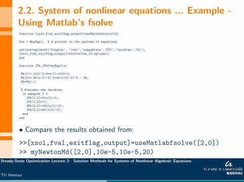
2.2. System of nonlinear equations ... Example -Using Matlab’s fsolvefunction [xsol,fval,exitflag,output]=useMatlabfsolve(x0)

fun = @myEqn1; % A pointer to the systems of equations

options=optimset(’Display’, ’iter’,’LargeScale’,’Off’,’Jacobian’,’On’);

[xsol,fval,exitflag,output]=fsolve(fun,x0,options);

end

function [Fk,JFk]=myEqn1(x)

Fk(1)= x(1)^2-2*x(1)-x(2)+1;

Fk(2)= 9*(x(1)-2)^2+4*(x(2)-2)^2 - 36;

Fk=Fk(:);

% Evaluate the Jacobian

if nargout > 1

JFk(1,1)=2*x(1)-2;

JFk(1,2)=-1;

JFk(2,1)=18*(x(1)-2);

JFk(2,2)=8*(x(2)-2);

end

end

• Compare the results obtained from:

>>[xsol,fval,exitflag,output]=useMatlabfsolve([2,0])

>> myNewtonMd([2,0],10e-5,10e-5,20)Steady-State Optimization Lecture 2: Solution Methods for Systems of Nonlinear Algebraic Equations

TU Ilmenau

2.3. Properties of the Newton Algorithm - speed ofconvergence• The speed of convergence towards the solution x∗ is one measure of quality for an iterative numerical

algorithm.

I Let x0, x1, . . . , xk , xk+1, . . . are iterates generated by an algorithm to solve a system of equations (or

an optimization problem).

Quadratic Convergence:

If the sequence of iterates xk converges to x∗ and there is a constant K > 0 such that

‖xk+1 − x∗‖ ≤ K‖xk − x∗‖2, k = 0, 1, 2, . . . ,

then the algorithm is said to be quadratically convergent or has a quadratic convergence.

Super-linear Convergence:

If the sequence of iterates xk converges to x∗ in such a way that

‖xk+1 − x∗‖ ≤ γk‖xk − x∗‖, k = 0, 1, 2, . . . ,

and limk→∞ γk = 0, then the algorithm is said to be super-linearly convergent or has a super-linear

convergence.

Linear Convergence:

If the sequence of iterates xk converges to x∗ and there is a constant K such that

‖xk+1 − x∗‖ ≤ γ‖xk − x∗‖, k = 0, 1, 2, . . . ,

where γ ∈ (0, 1), then the algorithm is said to be linearly convergent or it has a linear convergence.


TU Ilmenau

2.3. Properties of the Newton Algorithm ...

• Quadratic convergence is the fastest.• Any quadratic convergent sequence is super-linear convergent, and a super-linearconvergent sequence has also the linear convergence property.

Convergence Properties of the Newton Algorithm:Let U(x∗) be some neighborhood of the solution x∗. If:• the Jacobian of F (x) has a bounded inverse,i.e.

‖J−1F (x)‖ ≤ K , for all x ∈ U(x∗)

• and the Jacobian of JF (x) is Lipschitz continuous in U(x∗); i.e. there is a constantL > 0 such that

‖J(x1)− J(x2)‖ ≤ L‖x1 − x2‖, for any x1, x2 ∈ U(x∗)

then the Newton Algorithm:I is convergent to the solution x∗ from any initial iterate x0 in U(x∗), and

I the convergence is quadratic.


TU Ilmenau

2.3. Properties of the Newton Algorithm

• Note that, the Newton Algorithm is guaranteed to converges fast if the initialiterate x0 is near to the solution x∗.• If the initial iterate x0 is chosen far from the solution x∗, then the NewtonAlgorithm may either require too many iteration to converge and it may not evenconverge.

Example: Execute the following command and see what happens:

>>myNewton2(100,10e-5,10e-5,20)

• The Newton Algorithm is a locally convergent algorithm.• Hence, the iteration xk+1 = xk + dk , where JF (xk)dk = −F (xk) is known as thelocal Newton Method.

A Major Disadvantage of the Newton Method:• Since the location of the solution x∗ may not be known, it is generally difficult tochoose an initial iterate x0 near to x∗.


TU Ilmenau

2.4. Modifications of the Newton Algorithm• The local Newton Algorithm should be modified so that it is possible to choosean arbitrary initial iterate x0.• Such modifications of the Newton Algorithm are known as globalized NewtonMethods (Algorithms).• There are several modifications of the local Newton Algorithm to make itglobally convergent.

Globalization by using step-lengths• One method of globalization of the Newton Algorithm is to use step-lengths.• Instead of xk+1 = xk + dk we use

xk+1 = xk + αkdk ,

where αk is known as a step-length to be determined at each iteration.

Requirement:(sufficient decrease condition)Each new iterate should be determined in such a way that

‖F (xk+1)‖2 ≤ (1− σαk) ‖F (xk)‖2, σ is a given constant.

• This requirement guarantees that the norm ‖F (x)‖ reduces sufficiently from

iteration to iteration, until convergence.


TU Ilmenau

2.4. Modifications of the Newton Algorithm ...

I Note that, if we define f (x) = 12‖F (x)‖2. The requirement above implies that

f (xk + αkdk ) =1

2‖F (xk+1)‖2 ≤

1

2(1− σαk )︸︷︷︸≤1

‖F (xk )‖2 ≤1

2‖F (xk )‖2 = f (xk ).

This implies f (xk + αkdk ) ≤ f (xk ). Hence, dk is a decent direction for f (x) = 12‖F (x)‖2.

Question:How to choose the step-length αk?I If α1 = 1 and xk+1 = xk + dk satisfy the requirement, then αk = 1 is always agood choice.I Otherwise, choose an αk so that 0 < αk < 1.


TU Ilmenau

2.4. Modifications of the Newton Algorithm ...Algorithm 3: A Modified Newton Algorithm for solving F (x) = 0

1: Choose an initial iterate x0;

2: Choose initial step-length α0 = 1 and constants σ ∈(0, 1

2

), λ ∈ (0, 1).

3: Set k ← 0;4: while (‖F (xk )‖ ≥ tol) do5: Compute F (xk ) and JF (xk );

6: Set αk = min{1, αkλ};

7: Solve the systems of linear equations

JF (xk )d = −F (xk );


xk+1 = xk + αkdk ;

9: while (‖F (xk+1)‖2 > (1− 2σαk ) ‖F (xk )‖2) do10: Reduce αk = λ · αk ;11: New iterate xk+1 = xk + αkdk ;12: end while13: Set k ← k + 1;14: end while


TU Ilmenau

2.4. Modifications of the Newton Algorithm ...

• In the modified Newton Algorithm the requirement

‖F (xk+1)‖2 < (1− 2σαk ) ‖F (xk )‖2 , σ ∈(

0,1

2

)is known as Armijo-Rule.• Commonly used constants are λ = 0.5 and either σ = 10−4 or σ = 10−2.


TU Ilmenau

2.4. Modifications of the Newton Algorithm...Matlab

Matlab implementation of the modified Newton Algorithm:


TU Ilmenau

2.4. Modified Newton Algorithm ...ExampleExample: Configuring a robot arm so that it rests at a prescribed steady-state position is an importantproblem in industrial robotic applications.An idealized two-link robot arm consists of two rods, `1 = 2m and `2 = 3m, that are joined end-to-endin the plane. The robot arm is free to rotate w.r.t. the joints. The base of the robot arm is assumedfixed at the origin (0, 0) the coordinate plane. Find a spatial configuration of rods, so that the robot’sare comes to rest at the prescribed position R = (r1, r2) with coordinates (5, 5).

Note: A realistic industrial robot-arm has more than two links. As a result, there are infinitely manypossible configurations. The robot-arm here has only two possible configurations, we would like todetermine at least one of the configurations by applying the modified Newton Algorithm.


TU Ilmenau

2.4. Modified Newton Algorithm ...Example

Solution:Coordinates of the terminal-points of the rods are

P1 : (`1 cosα, `1 sinα), (3)

P2 : (`2 cosβ, `2 sinβ). (4)

Hence, the free-end of the robot-arm is at the pointP1 + P2 = (`1 cosα+ `2 cosβ, `1 sinα+ `2 sinβ). Thus we need to solve the system ofequations:

`1 cosα+ `2 cosβ = r1 =⇒ 2 cosα+ 3 cosβ = 5 (5)

`1 sinα+ `2 sinβ = r2 =⇒ 2 sinα+ 3 sinβ = 5. (6)

Solve these equations for α and β.It is easy to find the Jacobi matrix

J(α, β) =

[−2 sinα −3sinβ2 cosα 3 sinβ

]


TU Ilmenau

2.4. Nonlinear equations ... Example - CSTRExample:(Ref: Numerical Method for Chemical Engineering by Kenneth J. Beers, Cambridge University Press, 2007.)In a continuously steered reactor (CSTR), two elementary chemical reactions are takingplace isothermally and with a negligible volume change.

A + B −→ C rR1 = k1cAcBC + B −→ D rR2 = k2cC cB .

The mixture is assumed to be perfectly mixed with a uniform concentration of eachspecies in the reactor.


TU Ilmenau

2.2. Nonlinear equations ... Example - CSTR...The governing mass-balance equations are

VcA= q

(cA,in − cA

)+ V (−k1cAcB )

VcB= q

(cB,in − cA

)+ V (−k1cAcB − k2cC cB )

VcC= q

(cC,in − cC

)+ V (k1cAcB − k2cC cB )

VcD= q

(cD,in − cD

)+ V (k2cC cB ) .

The objective is to find the concentrations cA, cB , cC and cD at steady-state. Hence, we need to solve system ofequations

0 = q(cA,in − cA

)+ V (−k1cAcB )

0 = q(cB,in − cA

)+ V (−k1cAcB − k2cC cB )

0 = q(cC,in − cC

)+ V (k1cAcB − k2cC cB )

0 = q(cD,in − cD

)+ V (k2cC cB )

where

q = 1 volumetric flow rateV = 100 fixed reactor volume

cA,in = 1, cB,in = 2, cc,in = 0 and cD,in = 0 input (inlet) concentration of species

k1 = 1 and k2 = 1 reaction rate constants


TU Ilmenau

2.4. Nonlinear equations ... Example - CSTR...Solution:Define x1 = cA, x2 = cB , x3 = cC and x4 = cD and use the given constants to obtain

(1− x1) + 100 (−x1x2) = 0

(2− x2) + 100 (−x1x2 − x3x2) = 0

(0− x3) + 100 (x1x2 − x3x2) = 0

(0− x4) + 100 (x3x2) = 0.

Which is written equivalently as

x1 − 100x1x2 + 1 = 0

−x2 − 100x1x2 − 100x2x3 + 2 = 0

−x3 + 100x1x2 − 100x2x3 = 0

−x4 + 100x2x3 = 0

The analytic representation of the Jacobian matrix will be

J(x) =

1− 100x2 −100x1 0 0

−100x26− 1− 100(x1 + x3) −100x2 0100x2 100(x1 − x3) −1− 100x2 0

0 100x3 100x2 −1


TU Ilmenau

2.2. Nonlinear equations ... Example - CSTR...

Solution:Matlab Codes for the solution of the problem.


TU Ilmenau

2.4. Modified Newton Algorithm...PropertiesProperties of the Modified Newton Algorithm:• If the vector function F (x) is two-times differentiable and the Jacobi matrix JF (x) isinvertible at each point x , then:I an arbitrary initial iterate x0 can be chosen.I The sequence of iterates {xk} converges to the solution x∗ super-linearly; i.e. there is asequence {γk}

‖xk+1 − x∗‖ ≤ γk‖xk − x∗‖with limk→∞ γk = 0.I after a certain number of iterations, it is possible to chose a step-length of αk = 1,(i.e. the modified Newton Algorithm behaves just like the Newton Algorithm near to thesolution)

Disadvantages of the Newton and globalized Newton Methods:

D1: The Jacobian JF (x) is required to have an analytic expression or be exactlycomputable.D2: Good convergence properties are guaranteed if the Jacobian matrix JF (x) is invertible.D3: At each iteration step k, the system of linear equations JF (xk )d = −F (xk ) should beexactly solved in order to obtain dk .

I These are serious issues when solving large-scale system of nonlinear equations inpractical engineering applications.I For large-scale system of nonlinear equations, the direct computation of the Jacobiancould take enormous cpu-time.


TU Ilmenau

2.5. Newton Methods with Approximate JacobianI Three frequently used methods to approximately compute the Jacobian:(i) Finite difference approximation(ii) Quasi-Newton Methods(iii) Automatic differentiation - will not be discussed in this course (Ref: Evaluating derivatives :

principles and techniques of algorithmic differentiation by A. Griewank and A. Walther, SIAM 2008.).

(i) Finite difference (FD) approximation:

(a) Forward difference approximation

∂Fi (xk )

∂xj≈

Fi (xk + hjej )− Fi (xk )

hj, j = 1, . . . , n; i = 1, . . . , n.

I In the forward FD approximation the choice of h′j s is a trade-off between requiredcomputational accuracy and cpu-time.I Good Jacobian approximation is obtained for smaller values of the hj ’s. But, too-smallvalues for the h′j s may cause round-off errors.

I Sometimes the hj ’s can be chosen adaptively at each iteration step so that we use h(k)j

in place of hj . One approach is

h(k)j =

√εM

{ ∣∣∣x(k)j

∣∣∣ ,Mj

}sign{xkj }, where εM and Mj are constants.


TU Ilmenau

2.5. Newton Methods with Approximate Jacobian(b) Central difference approximation

∂Fi (xk )

∂xj≈

Fi (xk + hjej )− Fi (xk − hjej )

2hj, j = 1, . . . , n; i = 1, . . . , n.

for sufficiently small fixed values of hj , j = 1, . . . , n; where ej ∈ Rn is the j-th unit vector.

Advantages:I The FD approximation of the Jacobian is simple to implement.I It may provide good approximate Jacobian for small- to medium-scale system ofnonlinear equations F (x) = 0 with weaker nonlinearities.

Disadvantages:I Jacobian from FD may not be accurate and may lead numerical instability.I It is difficult to a-priori select the optimal finite difference step length hj , j=1,. . . ,nI For large-scale system of equations F (x) = 0, the cost of function evaluation (requiredcpu-time and memory) can be expensive (i.e. evaluation of F (x(k)),F (x(k) + hjej ) andF (x(k) − hjej )).

⇒ Despite their simplicity, FD methods are not widely used for the approximation of

JF (x) in the solution of large-scale F (x) = 0.


TU Ilmenau

2.5. ...Quasi-Newton Methods• Let f : R→ R be a differentiable scalar valued function of a scalar variable.• Given two numbers xn+1 and xn, the derivative f ′ at xn+1 can be approximated by

bn+1 =f (xn+1)− f (xn)

xn+1 − xn.

The value bn+1 is known as the secant approximation of the derivative f ′(xn+1).

Analogy:(secant approximation of the Jacobian J(x(k+1)))

Bk+1

(x(k+1) − x(k)

)= F (x(k+1))− F (x(k))

The matrix Bk+1 is the secant approximation of the Jacobian JF (x(k+1)).

Question: How to determine Bk+1 at each iteration step?

I There are several approaches.

The Broyden Method: Given Bk find

Bk+1 = Bk +(yk − Bkdk ) d>k

d>k dk,

where yk = F (x(k+1))− F (x(k)) and sk = x(k+1) − x(k) = αkdk .


TU Ilmenau

2.5. ...Quasi-Newton MethodsAlgorithm 4: Broyden’s Method1: Choose an initial iterates x0 and B0 ;2: Choose initial step-length α0.3: Set k ← 0;4: while (‖F (xk )‖ > tol) and (k < maxIter) do5: Compute F (xk );6: Choose αk ;7: Solve the systems of linear equations

Bkd = −F (xk );


xk+1 = xk + αkdk ;

9: Compute sk = x(k+1) − x(k);

10: Compute yk = F (x(k+1))− F (x(k));

11: Compute Bk+1 = Bk +(yk−Bkdk )d>k

d>k

dk;



TU Ilmenau

2.5. ...Properties the Brydon MethodI Often B0 = JF (x(0)).I If no step-length adjustment is used (i.e. αk = 1 and xk+1 = xk + dk ), then

− when the initial iterate x(0) is far from x∗, it may not converge;− local superlinear converges is guaranteed if ‖x(0) − x∗‖ ≤ δ and ‖B0 − JF (x(0))‖ ≤ ε forsome constants δ > 0 and ε > 0.I To guarantee global convergence, the step-length αk = 1 need to be adjustment at eachiteration.

Advantages:• QN provides a cheaper approximation of the Jacobian. There is no need to save matrices.• Sometimes Quasi-Newton Methods are also called Jacobian-free Methods

Disadvantages:

• Even if the Jacobian J(x(k)) is a sparse-matrix, the Brydon approximation Bk can bedense.• Hence, working the storage of the full matrix Bk may consume memory space. (Hence,

limited memory Quasi-Newton Methods).⇒ For large-scale equations with sparse Jacobians, the Broyden methods needs to bemodified.

• For a large-scale system of nonlinear equations F (x) = 0, the solution of the systemof linear equations

Bkd = −F(x(k)

)may take too much of the cpu-time.


TU Ilmenau

2.6. Inexact Newton Methods

• When the Jacobian matrix JF (x) is large and sparse, it may be difficult to solve the

equation JF (xk )d = −F (xk ).

⇒ Finding dk so that JF (xk )d + F (xk ) = 0 exactly, consumes most of the computation

time.• Instead:− use an iterative solver, e.g. CG, GMRES, etc., (see Lecture Slides 1) on the equationJF (xk )d = −F (xk ).− run the linear solver for a given number of iterations N to obtain a dk .• In this way obtained vector dk may not solve JF (xk )d = −F (xk ) exactly. Hence, there isa residual rk

rk = JF (xk )dk + F (xk )

• In order to guarantee that the new iterate xk + dk is better than xk we require

‖JF (xk )dk + F (xk )‖ ≤ ηk ‖F (xk )‖ , k = 0, 1, 2, . . . (7)

where ηk > 0 is a constant known as the forcing term.• Equation (7) guarantees that (forces) the iterates {xk} to converge to the solution ofF (x) = 0.I A Newton Algorithm with the above strategy for the determination of thesearch-directions dk is known as an Inexact Newton Method.


TU Ilmenau

2.6. Inexact Newton Methods...Algorithm 5: A general Inexact Newton Algorithm1: Choose an initial iterates x0 and a sequence {ηk} ;2: Set k ← 0;3: while (not convergence) do4: Compute JF (xk ) and F (xk )5: Determine the search direction dk so that

‖JF (xk )dk + F (xk )‖ ≤ ηk ‖F (xk )‖

6: Compute the next iterate:xk+1 = xk + dk ;

7: Set xk ← xk+1;8: Set k ← k + 1;9: end while

Questions:• What is a good choice for ηk at each iteration k?• How to determine dk ?

I The termination-criteria for the algorithm above usually checks if ‖F (xk )‖ ≤ tol issatisfied, for a sufficiently small user-defined number tol .


TU Ilmenau

2.6. Inexact Newton Methods...Strategies for choosing ηk :• In general, chose ηk so that 0 ≤ ηk ≤ 1.• Eisenstat and Walker 1996 suggest to use any one of the following:

Choice 1:

ηk =‖F (xk )− F (xk−1)− JF (xk )dk−1‖

‖F (xk−1)‖, k = 1, 2, . . .

Choice 2:

ηk =‖F (xk )‖ − ‖F (xk−1)− JF (xk )dk−1‖

‖F (xk−1)‖, k = 1, 2, . . .

Choice 3:

ηk = γ

(‖F (xk )‖‖F (xk−1)‖

)α, k = 1, 2, . . .

where γ ∈ [0, 1] and α ∈ (1, 2] are constants.

Strategies for finding dk :• Inexact Newton Methods are used for large-scale systems.• So use any of the Krylov-subspace methods on JF (xk )d = −F (xk ) to determine a dk .• Modern implementations frequently use the GMRES on JF (xk )d = −F (xk ) withappropriate pre-conditioners.I A Newton Method with a Krylov solver for JF (xk )d = −F (xk ) is commonly known as aNewton-Krylov Algorithm.


TU Ilmenau

2.6. Inexact Newton Methods...Algorithm 6: A Newton Krylov Algorithm1: Choose an initial iterates x0 and tolerance tol ;2: Set γ = 0.9, ηmax = 0.9999, ηmin = 10−4, ηold = ηmax ;3: Set k ← 0;4: while (‖F (xk )‖ > tol) do5: Compute JF (xk ) and F (xk ) ;6: Use the GMRES method to solve the equation JF (xk )d = −F (xk ) and obtain dk ;7: Compute the next iterate xk+1 = xk + dk ;

8: Compute η = γ ∗(‖F (xk+1)‖‖F (xk )‖

)2;

9: if (γ ∗ η2old < 0.1) then

10: η = min{η, ηmax}11: else12: η = min

{ηmax ,max{η, γ ∗ η2

old}}

13: end if14: Set xk ← xk+1;15: Set ηold ← η;16: Set k ← k + 1;17: end while

• The IF - ElLSE block above defines a so-called safeguard.• The safeguard tries to avoid too small values of ηk which may incur unnecessary additional iterations.• The suggestion for a safeguard step was mad by Einsenstat and Walker 1996 based on their experimental observations.


TU Ilmenau

2.6. Inexact Newton Methods...Properties

• In general, the Inexact Newton Algorithm is only locally convergent.• For global convergence, it may be necessary to use a step-length.• The convergence of the Inexact Newton Algorithm is usually linear.• But, if limk→∞ ηk = 0, then the convergence is (local) superlinear.• The direct computation of the Jacobian JF (xk) can be avoided byusing the Quasi-Newton (Broyden type) methods for theapproximation of the Jacobian at each iteration.

Other Important Methods for Nonlinear Equations:I Limited Memory Quasi-Newton MethodsI Newton Methods with Trust RegionI Tensor Newton MethodsI Homotopy or Continuation Methods


TU Ilmenau

References1 R.S Dembo; S.C. Einsenstat; T. Steihaug: Inexact Newton methods. SIAM J. Sci.

Comput., 19(1), pp. 400–408, 1982.

2 J.E. Dennis,JR; R.B. Schanabel: Numerical methods of unconstrained optimizationand nonlinear equations. Prentice-Hall,Englewood-Cliffs, 1983.

3 P. Deufelhard: Newton methods for nonlinear problems: affine invariance andadaptive algorithms. Springer, 2004.

4 S.C. Einsenstat; H.F. Walker: Choosing the forcing terms in an inexact Newtonmethod. SIAM J. Sci. Comput., 17(1), pp. 16-32, 1996.

5 A. Hoffmann; B. Marx, W. Voigt: Mathematik fur Ingenieure 1. Pearson Studium,2005.

6 C. T. Kelley: Solving nonlinear equations with Newton methods. SIAM,Philadelphia, 2003.

7 C. T. Kelley: Iterative Methods for Linear and Nonlinear Equations. SIAM,Philadelphia, 1995.

8 P. Kosmol: Method zur numerischen Behandlung nichtlinearer Gleichungen undOptimierungsaufgaben. Teubner-Verlag, Stuttgart, 1989.

9 J.M. Ortega und W.C. Rheinboldt: Iterative Solution of Nonlinear Equations inSeveral Variables. Academic Press, 1970.

10 H. Schwetlick: Numerische Losung nichtlinearer Gleichungen. Oldenbourg-Verlag,1979.


TU Ilmenau

Software Resurces

1 M. Pernice; H.F. Walker NITSOL: A Newton iterative solver for nonlinear systems(http://users.wpi.edu/ walker/NITSOL/).

2 C. T. Kelley: MATLAB codes for solving nonlinear equations with Newton’s method(http://www4.ncsu.edu/ ctk/newtony.html).

3 R.J. Spiteri; T.-P. Ter: pythNon: A PSE for numerical solution of nonlinear algebraicequations. Journal of Numerical Analysis, 3(1-2), pp. 127-137, 2008.(Numerical Simulation Research Lab, University of Saskatchewan,URL: http://simcity.usask.ca/?page_id=476)

4 Software repository for Peter Deuflhards Book : Newton Methods for NonlinearProblems - Affine Invariance and Adaptive Algorithms.(Numerical Analysis and Modelling - NewtonLib, Konrad-Zuse-Zentrum furInformationstechnik, Berlin.URL: http://www.zib.de/?id=818)


TU Ilmenau

steady-state optimization lecture 2: solution methods for ... · nonlinear algebraic equations...

Documents