research article optimal application timing of pest...
TRANSCRIPT

Research ArticleOptimal Application Timing of Pest Control Tactics inNonautonomous Pest Growth Model
Shujuan Zhang Juhua Liang and Sanyi Tang
College of Mathematics and Information Science Shaanxi Normal University Xirsquoan 710062 China
Correspondence should be addressed to Juhua Liang juhualiang81gmailcom
Received 28 March 2014 Accepted 25 May 2014 Published 25 June 2014
Academic Editor Shengqiang Liu
Copyright copy 2014 Shujuan Zhang et alThis is an open access article distributed under the Creative Commons Attribution Licensewhich permits unrestricted use distribution and reproduction in any medium provided the original work is properly cited
Considering the effects of the living environment on growth of populations it is unrealistic to assume that the growth rates ofpredator and prey are all constants in the models with integrated pest management (IPM) strategies Therefore a nonautonomouspredator-prey system with impulsive effect is developed and investigated in the present work In order to determine the optimalapplication timing of IPM tactics the threshold value which guarantees the stability of pest-free periodic solution has been obtainedfirstlyThe analytical formula of optimal application timings within a given period for different cases has been obtained such that thethreshold value is the smallest which is themost effective in successful pest control Moreover extensively numerical investigationshave also been confirmed our main results and the biological implications have been discussed in more detailThemain results canguide the farmer to design the optimal pest control strategies
1 Introduction
Recently many ecologists are becoming increasingly con-cerned with the questions of pest control and designing theoptimal control strategies It is well known that the pesticidesare still the main tactics for controlling pests because thepesticides are relatively cheap and can be easily appliedBut spraying insecticides for a long time may trigger ldquo3Rrdquoquestions (resistance resurgence and residue) then theDepartment of Agricultural Ecology proposed the integratedpest management (IPM) strategies [1 2]
IPM is a long term management strategy which includeschemical (insecticides) biological (releasing the naturalenemy) agricultural control (crop rotation) and physicsmethods (utilizing light to trap and kill pest) [3 4] IPMwhich has been proved by experiment is more effective thanany single control strategy But when should we release thenatural enemy and what proportion do we need to kill thepest by spraying pesticide Undoubtedly the mathematicalmodels can help us to design the optimal control tacticsand in particular help us to predict the density of pestpopulation and to determine optimal application timing ofIPM strategies (see [5ndash8])
Volterra first proposed a simple predator-prey systemwhich has been extended and modified in many ways [9 10]
In recent years continuous or discrete predator-prey systemsconcerning IPM strategies have been developed and inves-tigated intensively in [11ndash13] Considering the interventionsby human such as a periodic spraying pesticide and aconstant periodic releasing for the predator the impulsivedifferential equations with fixed moments were employed tomodel the interventions and consequently the Lotka-Volterrasystem has been extended [14] However one of the majorassumptions in those publications was that all the growthrates of predator and prey are constants However manyecologists have shown that the growth of populations ofvarious species is affected by the special living environmentincluding the seasons weather conditions and food supply[15] Therefore it is more realistic to consider the effectsof periodic parameters on the dynamics of predator-preymodels Therefore nonautonomous predator-prey systemswith impulsive effect have been developed and investigatedin [10 16 17]
However those works mainly focused on the effectsof periodic perturbations on the dynamics the interestingquestions concerning the effects of successful pest control inparticular how to apply the IPM tactics in periodic environ-ment and to determine the optimal application timing havenot been addressed in more detail
Hindawi Publishing CorporationAbstract and Applied AnalysisVolume 2014 Article ID 650182 12 pageshttpdxdoiorg1011552014650182
2 Abstract and Applied Analysis
Thus in the present work a nonautonomous predator-prey model with periodic perturbations and periodic impul-sive effects is developed and investigated Firstly the stabilityof pest-free periodic solution and its threshold condition havebeen investigated which can be used for determining theoptimal timing of IPM applications Secondly we assumethat only one-impulsive controlling has been applied withina given period and the optimal application timing hasbeen determined and consequently the analytical formula isalso provided under which the threshold value reaches itsminimum Then we assume that two-impulsive controllingor more impulsive controlling has been applied within agiven period and similarly the optimal time points and theiranalytical formula have also been obtained and providedMoreover the biological implications have been discussed inmore detail Finally some numerical simulations concerningthe main results have been done We conclude that themain results can help us to design the optimal pest controlstrategies
2 The Periodic Integrated PestControl Strategies
21 Autonomous ODE Model with Multi-Impulsive EffectsAssume that the pest population follows the classical logisticgrowth system and that pest control by spraying pesticidesand releasing natural enemies is implemented at some fixedtimes for each crop season Denote the size of the pest andthe natural enemy populations at time 119905 by 119909(119905) and 119910(119905)respectively Assume that pests are killed by pesticides at aproportional rate 119901119896 (0 le 119901119896 lt 1) and the natural enemyis released by a constant 120590 at time 120591119896 Therefore we have thefollowing system with impulsive effects at fixed moments
119889119909 (119905)
119889119905= 119903119909 (119905) [1 minus 119886119909 (119905)] minus 119887119909 (119905) 119910 (119905)
119889119910 (119905)
119889119905= 119910 (119905) [119888119909 (119905) minus 120575]
119905 = 120591119896 (119896 = 1 2 )
119909 (120591+
119896) = (1 minus 119901119896) 119909 (120591119896)
119910 (120591+
119896) = 119910 (120591119896) + 120590
119905 = 120591119896
(1)
where 119903 is the intrinsic growth rate of pest population 119886denotes the carrying capacity parameter 119887 is the attack rateof predator 119888 represents conversion efficiency and 120575 is thedeath rate of predator System (1) is said to be a 119879 periodicsystem if there exists a positive integer 119902 such that 119901119896+119902 = 119901119896120591119896+119902 = 120591119896 + 119879 This implies that in each period 119879 119902 times ofthe pesticide applications are used and 119902 times of the naturalenemy releases are applied
The dynamical behavior and biological implications ofsystem (1) have been extensively studied in [18] It followsfrom the literature [18] that if exp(minus120575119879) lt 1 then system (1)
has a ldquopest-eradicationrdquo periodic solution (0 119910119879(119905)) over the
119899th time interval 119899119879 lt 119905 le (119899 + 1)119879 with
119910119879(119905) =
119884lowast exp [minus120575 (119905 minus 119899119879)]
119905 isin (119899119879 119899119879 + 1205911]
119884lowast exp [minus120575 (119905 minus 119899119879)]
+120590
119896
sum
119895=1
exp [minus120575 (119905 minus 119899119879 minus 120591119895)]
119905 isin (119899119879 + 120591119896 119899119879 + 120591119896+1]
119884lowast exp [minus120575 (119905 minus 119899119879)]
+120590
119902
sum
119895=1
exp [minus120575 (119905 minus 119899119879 minus 120591119895)]
119905 isin (119899119879 + 120591119902 (119899 + 1) 119879]
(2)
where 119884lowast
= (120590sum119902
119895=1exp(minus120575(119879 minus 120591119895)))(1 minus exp(minus120575119879)) and
(0 119910119879(119905)) is globally asymptotically stable provided that 1198770 lt
1 with
1198770 ≜
119902
prod
119894=1
(1 minus 119901119894) exp(119903119879 minus119887119902120590
120575) (3)
The analytical formula defined above clearly shows howthe key parameters affect the threshold value 1198770 which canbe used to design the optimal control strategies such thatthe threshold value 1198770 is the smallest We will address thosepoints in the following for more generalized model
22 Nonautonomous ODE Model with Multi-Impulsive Ef-fects However it is well known that the growth of popula-tions of various species is affected by several factors such asthe seasons weather conditions and food supply which canbe described by using the periodic coefficients in model (1)that is we have the following model
119889119909 (119905)
119889119905= 119903 (119905) 119909 (119905) [1 minus 119886 (119905) 119909 (119905)] minus 119887 (119905) 119909 (119905) 119910 (119905)
119889119910 (119905)
119889119905= 119910 (119905) [119888 (119905) 119909 (119905) minus 120575 (119905)]
119905 = 120591119896
119909 (120591+
119896) = (1 minus 119901119896) 119909 (120591119896)
119910 (120591+
119896) = 119910 (120591119896) + 120590119896
119905 = 120591119896
(4)
where 119903(119905) 119886(119905) 119887(119905) 119888(119905) and 120575(119905) are continuous 119879 periodicfunctions System (4) is said to be a 119879 periodic system if thereexists a positive integer 119902 such that 119901119896+119902 = 119901119896 120590119896+119902 = 120590119896 and120591119896+119902 = 120591119896 + 119879
Abstract and Applied Analysis 3
In order to analyze the dynamics of the pest populationin system (4) the following subsystem is useful
119889119910 (119905)
119889119905= minus120575 (119905) 119910 (119905) 119905 = 120591119896
119910 (120591+
119896) = 119910 (120591119896) + 120590119896 119905 = 120591119896
(5)
and we have the following main results for subsystem (5)
Lemma 1 The subsystem (5) has a positive periodic solution119910119879(119905) and for every solution119910(119905) of (5) one has |119910(119905)minus119910119879(119905)| rarr
0 as 119899 rarr infin where
119910119879(119905) =
119884lowast
119899exp [minusint
119905
119899119879
120575 (119904) 119889119904]
119905 isin (119899119879 119899119879 + 1205911]
119884lowast
119899exp [minusint
119905
119899119879
120575 (119904) 119889119904]
+
119896
sum
119895=1
120590119895 exp[minusint
119905
119899119879+120591119895
120575 (119904) 119889119904]
119905 isin (119899119879 + 120591119896 n119879 + 120591119896+1]
119884lowast
119899exp [minusint
119905
119899119879
120575 (119904) 119889119904]
+
119902
sum
119895=1
120590119895 exp[minusint
119905
119899119879+120591119895
120575 (119904) 119889119904]
119905 isin (119899119879 + 120591119902 (119899 + 1) 119879]
(6)
119884lowast
119899=
sum119902
119895=1120590119895 exp [minus int
(119899+1)119879
119899119879+120591119895120575 (119904) 119889119904]
1 minus exp [minus int(119899+1)119879
119899119879120575 (119904) 119889119904]
(7)
119899 isin N andN = 0 1 2
Proof In any given time interval (119899119879 (119899 + 1)119879] (where 119899 isa natural number) we investigate the dynamical behavior ofsystem (5) In fact integrating the first equation of system (5)from 119899119879 to 119899119879 + 1205911 yields
119910 (119905) = 119910 (119899119879) exp [minusint
119905
119899119879
120575 (119904) 119889119904] 119905 isin (119899119879 119899119879 + 1205911]
(8)
At time 119899119879 + 1205911 the 1205901 natural enemy is released thus wehave
119910 ((119899119879 + 1205911)+) = 119910 (119899119879) exp [minusint
119899119879+1205911
119899119879
120575 (119904) 119889119904] + 1205901 (9)
Again integrating the first equation of system (5) from 119899119879+1205911
to 119899119879 + 1205912 one yields
119910 (119905) = 119910 ((119899119879 + 1205911)+) exp [minusint
119905
119899119879+1205911
120575 (119904) 119889119904]
119905 isin (119899119879 + 1205911 119899119879 + 1205912]
(10)
At time 119899119879 + 1205912 the 1205902 natural enemy is released and
119910 ((119899119879 + 1205912)+) = 119910 (119899119879) exp [minusint
119899119879+1205912
119899119879
120575 (119904) 119889119904]
+ 1205901 exp [minusint
119899119879+1205912
119899119879+1205911
120575 (119904) 119889119904] + 1205902
(11)
By induction we get
119910 (119905) = 119910 (119899119879) exp [minusint
119905
119899119879
120575 (119904) 119889119904]
+
119902
sum
119895=1
120590119895 exp[minusint
119905
119899119879+120591119895
120575 (119904) 119889119904]
(12)
for all 119905 isin (119899119879 + 120591119902 (119899 + 1)119879] Therefore we have
119910 ((119899 + 1) 119879) = 119910 (119899119879) exp[minusint
(119899+1)119879
119899119879
120575 (119904) 119889119904]
+
119902
sum
119895=1
120590119895 exp[minusint
(119899+1)119879
119899119879+120591119895
120575 (119904) 119889119904]
(13)
Denote 119884119899+1 = 119910((119899 + 1)119879) then we have the followingdifference equation
119884119899+1 = 119884119899 exp[minusint
(119899+1)119879
119899119879
120575 (119904) 119889119904]
+
119902
sum
119895=1
120590119895 exp[minusint
(119899+1)119879
119899119879+120591119895
120575 (119904) 119889119904]
(14)
which has a unique steady state
119884lowast
119899=
sum119902
119895=1120590119895 exp [minus int
(119899+1)119879
119899119879+120591119895120575 (119904) 119889119904]
1 minus exp [minus int(119899+1)119879
119899119879120575 (119904) 119889119904]
(15)
Thus there is a periodic solution of system (5) denotedby 119910119879(119905) which is given in (6) For the stability of 119910119879(119905) it
follows from (12) and the formula of 119910119879(119905) that10038161003816100381610038161003816119910 (119905) minus 119910
119879(119905)
10038161003816100381610038161003816
=
10038161003816100381610038161003816100381610038161003816100381610038161003816
119910 (119899119879) exp [minusint
119905
119899119879
120575 (119904) 119889119904]
+
119896
sum
119895=1
120590119895 exp[minusint
119905
119899119879+120591119895
120575 (119904) 119889119904]
minus 119884lowast
119899exp [minusint
119905
119899119879
120575 (119904) 119889119904]
minus
119896
sum
119895=1
120590119895 exp[minusint
119905
119899119879+120591119895
120575 (119904) 119889119904]
10038161003816100381610038161003816100381610038161003816100381610038161003816
4 Abstract and Applied Analysis
=1003816100381610038161003816119910 (119899119879) minus 119884
lowast
119899
1003816100381610038161003816exp [minusint
119905
119899119879
120575 (119904) 119889119904]
997888rarr 0 as 119899 997888rarr infin
119905 isin (119899119879 + 120591119896 119899119879 + 120591119896+1]
(16)
and then the results of Lemma 1 follow This completes theproof of Lemma 1
Based on the conclusion of Lemma 1 there exists a ldquopest-freerdquo periodic solution of system (4) over the 119899th time interval119899119879 lt 119905 le (119899 + 1)119879 and we have the following thresholdconditions
Theorem 2 Let
1198770 =
119902
prod
119894=1
(1 minus 119901119894)
times exp[int
(119899+1)119879
119899119879
119903 (119905) 119889119905
minus
119902minus1
sum
119895=0
int
119899119879+120591119895+1
119899119879+120591119895
119887 (119905) 119910119879(119905) 119889119905
minusint
(119899+1)119879
119899119879+120591119902
119887 (119905) 119910119879(119905) 119889119905]
(17)
then the pest-free periodic solution (0 119910119879(119905)) of system (4) is
globally asymptotically stable if 1198770 lt 1
Proof Firstly we prove the local stability Define 119909(119905) = 119906(119905)119910(119905) = 119910
119879(119905) + V(119905) there may be written
(119906 (119905)
V (119905)) = Φ (119905) (119906 (0)
V (0)) (18)
where Φ(119905) satisfies
119889Φ
119889119905= (
119903 (119905) minus 119887 (119905) 119910119879(119905) 0
119888 (119905) 119910119879(119905) minus120575 (119905)
)Φ (119905) (19)
andΦ(0) = 119868 denoted the identitymatrixThe resetting of thethird and fourth equations of (4) becomes
(119906 (119899119879 + 120591
+
119896)
V (119899119879 + 120591+
119896)) = (
1 minus 119901119896 0
0 1)(
119906 (119899119879 + 120591119896)
V (119899119879 + 120591119896)) (20)
Hence if both eigenvalues of
119872 = (
119902
prod
119894=1
(1 minus 119901119894) 0
0 1
)Φ (119879) (21)
have absolute value less than one then the periodic solution(0 119910119879(119905)) is locally stable In fact the two Floquet multiplies
are thus
1205831 =
119902
prod
119894=1
(1 minus 119901119894) exp[int
(119899+1)119879
119899119879
(119903 (119905) minus 119887 (119905) 119910119879(119905)) 119889119905]
1205832 = exp[minusint
(119899+1)119879
119899119879
120575 (119905) 119889119905] lt 1
(22)
according to Floquet theory (see [19ndash21] and the referencestherein) the solution (0 119910
119879(119905)) is locally stable if |1205831| lt 1
that is if (17) holds true the solution of system (4) is locallystable
In the following we will prove the global attractivity of(0 119910119879(119905)) It follows from the second equation of system (4)
that we have119889119910(119905)119889119905 gt minus120575(119905)119910(119905) and consider the followingimpulsive differential equation
119889119906 (119905)
119889119905= minus120575 (119905) 119906 (119905) 119905 = 120591119896
119906 (120591+
119896) = 119906 (120591119896) + 120590119896 119905 = 120591119896
(23)
where 120575(119905) is continuous 119879 periodic function and 120590119896+119902 = 120590119896120591119896+119902 = 120591119896 + 119879
According to Lemma 1 and the comparison theorem onimpulsive differential equations we get 119910(119905) ge 119906(119905) and119906(119905) rarr 119910
119879(119905) as 119905 rarr infin Therefore
119910 (119905) ge 119906 (119905) gt 119910119879(119905) minus 120598 (24)
holds for 120598 (120598 gt 0) small enough and all 119905 large enoughWithout loss of generality we assume that (24) holds for all119905 ge 0 Thus we have
119889119909 (119905)
119889119905le 119903 (119905) 119909 (119905) minus 119887 (119905) 119909 (119905) [119910
119879(119905) minus 120598] 119905 = 120591119896
119909 (120591+
119896) = (1 minus 119901119896) 119909 (120591119896) 119905 = 120591119896
(25)
Again from the comparison theorem on impulsive differ-ential equations we get
119909 (119899119879 + 1205911)
le 119909 (119899119879) expint
119899119879+1205911
119899119879
[119903 (119905) minus 119887 (119905) (119910119879(119905) minus 120598)] 119889119905
119909 (119899119879 + 1205912)
le (1 minus 1199011) 119909 (119899119879 + 1205911)
times expint
119899119879+1205912
119899119879+1205911
[119903 (119905) minus 119887 (119905) (119910119879(119905) minus 120598)] 119889119905
Abstract and Applied Analysis 5
le (1 minus 1199011) 119909 (119899119879)
times exp
1
sum
119895=0
int
119899119879+120591119895+1
119899119879+120591119895
[119903 (119905) minus 119887 (119905) (119910119879(119905) minus 120598)] 119889119905
119909 ((119899 + 1) 119879)
le
119902
prod
119894=1
(1 minus 119901119894) 119909 (119899119879)
times exp
119902minus1
sum
119895=0
int
119899119879+120591119895+1
119899119879+120591119895
[119903 (119905) minus 119887 (119905) (119910119879(119905) minus 120598)] 119889119905
+ int
(119899+1)119879
119899119879+120591119902
[119903 (119905) minus 119887 (119905) (119910119879(119905) minus 120598)] 119889119905
=
119902
prod
119894=1
(1 minus 119901119894) 119909 (119899119879)
times expint
(119899+1)119879
119899119879
[119903 (119905) + 119887 (119905) 120598] 119889119905
minus
119902minus1
sum
119895=0
int
119899119879+120591119895+1
119899119879+120591119895
119887 (119905) 119910119879(119905) 119889119905
minusint
(119899+1)119879
119899119879+120591119902
119887 (119905) 119910119879(119905) 119889119905
≜ 119909 (119899119879) 119877120598
(26)
where 1205910 = 0 and
119877120598 =
119902
prod
119894=1
(1 minus 119901119894) expint
(119899+1)119879
119899119879
[119903 (119905) + 119887 (119905) 120598] 119889119905
minus
119902minus1
sum
119895=0
int
119899119879+120591119895+1
119899119879+120591119895
119887 (119905) 119910119879(119905) 119889119905
minusint
(119899+1)119879
119899119879+120591119902
119887 (119905) 119910119879(119905) 119889119905
(27)
Let 120598 rarr 0 we get the expression of1198770 which is given in (17)Therefore if 1198770 lt 1 then 119909(119899119879) le (1198770)
119899119909(0) Consequently
119909(119899119879) rarr 0 as 119899 rarr infinNext we can prove that 119910(119905) rarr 119910
119879(119905) as 119905 rarr infin For
any 120598 gt 0 there must exist a 1199051 gt 0 such that 0 lt 119909(119905) lt 120598 for119905 gt 1199051 Without loss of generality we assume that 0 lt 119909(119905) lt 120598
holds true for all 119905 gt 0 then we have
119889119910 (119905)
119889119905lt (120598119888 (119905) minus 120575 (119905)) 119910 (119905) (28)
and consider the following impulsive differential equation
119889V (119905)119889119905
= (120598119888 (119905) minus 120575 (119905)) V (119905) 119905 = 120591119896
V (120591+119896) = V (120591119896) + 120590119896 119905 = 120591119896
(29)
By using the same methods as those for system (23) it iseasy to prove that system (29) has a globally stable periodicsolution denoted by V119879(119905) and
V119879 (119905) =
Vlowast119899exp [int
119905
119899119879
(120598119888 (119904) minus 120575 (119904)) 119889119904]
119905 isin (119899119879 119899119879 + 1205911]
Vlowast119899exp [int
119905
119899119879
(120598119888 (119904) minus 120575 (119904)) 119889119904]
+
119896
sum
119895=1
120590119895 exp[int
119905
119899119879+120591119895
(120598119888 (119904) minus 120575 (119904)) 119889119904]
119905 isin (119899119879 + 120591119896 119899119879 + 120591119896+1]
Vlowast119899exp [int
119905
119899119879
(120598119888 (119904) minus 120575 (119904)) 119889119904]
+
119902
sum
119895=1
120590119895 exp[int
119905
119899119879+120591119895
(120598119888 (119904) minus 120575 (119904)) 119889119904]
119905 isin (119899119879 + 120591119902 (119899 + 1) 119879]
(30)
with
Vlowast119899=
sum119902
119895=1120590119895 exp [int
(119899+1)119879
119899119879+120591119895(120598119888 (119904) minus 120575 (119904)) 119889119904]
1 minus exp [int(119899+1)119879
119899119879(120598119888 (119904) minus 120575 (119904)) 119889119904]
(31)
Therefore combined with (24) for any 1205981 gt 0 there existsa 1199052 gt 0 such that 119910119879(119905) minus 1205981 lt 119910(119905) lt V119879(119905) + 1205981 for any 119905 gt 1199052Let 120598 rarr 0 then we have 119910
119879(119905) minus 1205981 lt 119910(119905) lt 119910
119879(119905) + 1205981 for
119905 gt 1199052 which indicates that 119910(119905) rarr 119910119879(119905) as 119905 rarr infin
This completes the proof of global attractivity of(0 119910119879(119905)) Then it is globally asymptotically stable The proof
of Theorem 2 is complete
3 The Optimal Control Time with Different 119902
Assume that pesticide is sprayed and the natural enemy isreleased only at the time points 119899119879 + 120591119894 (119894 = 1 2 119902 and0 lt 1205911 lt 1205912 lt sdot sdot sdot lt 120591119902 lt 119879) during each period 119879 It is wellknown that the size of the pest population at the end will bedifferent if impulsive control occurs at different time So itis necessary to determine the optimal time to make sure thatthe pest can be eliminated quickly
31 The Optimal Control Time with 119902 = 1 In this subsectionwe consider one-pulse controlling at time 119899119879 + 1205911 in eachperiod 119879 (where 1205911 isin [0 119879]) with aims to find the optimaltime 119899119879 + 1205911 such that the threshold value is the smallest
6 Abstract and Applied Analysis
Therefore if 119902 = 1 then the threshold value 1198770 can bereduced as
1198770 = (1 minus 1199011)
times exp[int
(119899+1)119879
119899119879
119903 (119905) 119889119905
minus int
119899119879+1205911
119899119879
119887 (119905) 119910119879(119905) 119889119905
minusint
(119899+1)119879
119899119879+1205911
119887 (119905) 119910119879(119905) 119889119905]
(32)
where
119910119879(119905) =
119884lowast
119899exp [minusint
119905
119899119879
120575 (119904) 119889119904]
119905 isin (119899119879 119899119879 + 1205911]
119884lowast
119899exp [minusint
119905
119899119879
120575 (119904) 119889119904]
+1205901 exp [minusint
119905
119899119879+1205911
120575 (119904) 119889119904]
119905 isin (119899119879 + 1205911 (119899 + 1) 119879]
119884lowast
119899=
1205901 exp [minus int(119899+1)119879
119899119879+1205911120575 (119904) 119889119904]
1 minus exp [minus int(119899+1)119879
119899119879120575 (119904) 119889119904]
(33)
Denote
119860 = int
(119899+1)119879
119899119879
119903 (119905) 119889119905
119861 (1205911) = 119884lowast
119899int
(119899+1)119879
119899119879
119887 (119905) exp [minusint
119905
119899119879
120575 (119904) 119889119904] 119889119905
1198621 (1205911) = 1205901 int
(119899+1)119879
119899119879+1205911
119887 (119905) exp [minusint
119905
119899119879+1205911
120575 (119904) 119889119904] 119889119905
(34)
Thus we have
1198770 = (1 minus 1199011) exp (119860 minus 119861 (1205911) minus 1198621 (1205911)) (35)
Taking the derivative of function 1198770 with respect to 1205911one obtains1198891198770
1198891205911
= minus (1 minus 1199011) (119889119861 (1205911)
1198891205911
+1198891198621 (1205911)
1198891205911
)
times exp (119860 minus 119861 (1205911) minus 1198621 (1205911))
= minus1198770 (119889119861 (1205911)
1198891205911
+1198891198621 (1205911)
1198891205911
)
= minus1198770 [120575 (119899119879 + 1205911) (119861 (1205911) + 1198621 (1205911)) minus 1205901119887 (119899119879 + 1205911)]
(36)
Letting 11988911987701198891205911 = 0 we can see that 1205911min satisfiesequation 119889119861(1205911)1198891205911 + 1198891198621(1205911)1198891205911 = 0 that is
1198661 ≐ 120575 (119899119879 + 1205911min) (119861 (1205911min) + 1198621 (1205911min))
minus 1205901119887 (119899119879 + 1205911min) = 0
(37)
The second derivative of 1198770 with respect to 1205911 at 1205911min can becalculated as follows
11988921198770
1198891205912
1
1003816100381610038161003816100381610038161003816100381610038161205911=1205911min
= minus1198770 [119889120575 (119899119879 + 1205911)
1198891205911
(119861 (1205911min) + 1198621 (1205911min))
minus 1205901
119889119887 (119899119879 + 1205911min)
1198891205911
]
= minus12059011198770 [119887 (119899119879 + 1205911min)
120575 (119899119879 + 1205911min)
119889120575 (119899119879 + 1205911)
1198891205911
1003816100381610038161003816100381610038161003816100381610038161205911=1205911min
minus119889119887 (119899119879 + 1205911)
1198891205911
1003816100381610038161003816100381610038161003816100381610038161205911=1205911min
]
(38)
If 119889211987701198891205912
1|1205911=1205911min
gt 0 that is 1205911min satisfies
119887 (119899119879 + 1205911min)
120575 (119899119879 + 1205911min)
119889120575 (119899119879 + 1205911)
1198891205911
|1205911=1205911min
minus119889119887 (119899119879 + 1205911)
1198891205911
|1205911=1205911min
lt 0
(39)
then 1205911min is the minimal value pointAccording to the above discussion we have the following
theorem
Theorem 3 If 1205911min satisfies (37) and inequality (39) then thethreshold value 1198770 reaches its minimum value
For example if we let 119903(119905) = 1199030 + 119886 cos(120596119905) 119887(119905) =
1198870 + 119887 sin(120596119905) and 120575(119905) = 1205750 + 1205751 cos(120596119905) then by simplecalculations we have
11988921198770
1198891205912
1
1003816100381610038161003816100381610038161003816100381610038161205911=1205911min
= 12059612059011198770 [1198871205751 + 12057511198870 sin (1205961205911min) + 1198871205750 cos (1205961205911min)
1205750 + 1205751 cos (1205961205911min)]
(40)
and if 1205911min satisfies
1198871205751 + 12057511198870 sin (1205961205911min) + 1198871205750 cos (1205961205911min)
1205750 + 1205751 cos (1205961205911min)gt 0 (41)
then 1205911min is the minimum value pointThat is 1198770 reaches itsminimum value when 1205911 = 1205911min
To confirm our main results obtained in this subsectionwe fixed all parameters including 119903(119905) 119886(119905) 119887(119905) 119888(119905) 120575(119905)1199011 1205901 and initial values 1199090 1199100 and carry out the numericalinvestigations To find the optimal timing of applying IPMstrategy we consider 11988911987701198891205911 as a function with respect to1205911 aiming to find the time point such that 11988911987701198891205911 = 0
Abstract and Applied Analysis 7
0 1 2 3 4 5minus02
minus015
minus01
minus005
0
005
01
015
1205911
1205911min = 095minusG1
Figure 1 Illustration of the existence of the minimal value pointThe parameter values are fixed as follows 119903(119905) = 15+03 cos(04120587119905)119887(119905) = 1 + 02 sin(04120587119905) 120575(119905) = 05 + 01 cos(04120587119905) 1205901 = 05 and1199011 = 025
Since 11988911987701198891205911 = minus11987701198661 = 0 we only need to plot the minus1198661
with respect to time 1205911 as shown in Figure 1 By calculationwe have 1205911min = 095 which satisfies inequality (41) andconsequently 1205911min is a minimum value point
Now we can consider the effects of different timing ofapplying IPM strategies on the pest population in particularthe amplitudes of the pest population To do this we choosethree different time points denoted by 1205911min 1205911 and 120591
1015840
1 at
which the one-time control action has been implementedIt follows from Figure 2 that the maximal value of the pestpopulation is the smallest when we implement the one-timecontrol action at time 1205911min which confirms that the resultsobtained here can help us to design the optimal controlstrategies
In the following we would like to address how theimpulsive period 119879 release quantity 1205901 pest killing rate 1199011and death rate of the pest population 119887(119905) affect the thresholdvalue 1198770 To address this question we fix the parametersconcerning periodic functions 119903(119905) 119886(119905) 119888(119905) and 120575(119905) andvary the impulsive period 119879 the release quantity 1205901 thekilling rate 1199011 and the death rate 119887(119905) respectively
In Figure 3 we see that the threshold value 1198770 is notmonotonic with respect to time 119905 and the effects of all fourparameters (119879 1205901 1199011 and 1198870) on threshold condition 1198770 arecomplex Figure 3(a) shows the effect of impulsive period 119879
on the1198770 and the results indicate that the larger the impulsiveperiod 119879 is the larger the threshold value is which will resultin a more sever pest outbreak Oppositely in Figure 3(b)the results indicate that the smaller the release quantity 1205901
is the larger the 1198770 is Figures 3(c) and 3(d) clarify thatslightly increasing the pest killing rate 1199011 and the death rateof pest 119887(119905) can reduce the quantity of threshold value 1198770
dramatically and the results can be used to help the farmerto select appropriate pesticides At the same time we can seeclearly how the periodic perturbations affect the thresholdvalue 1198770 as indicated in the bold curves in Figure 3
32 TheOptimal Control Time with 119902 = 2 In this subsectionwe consider two-pulse controlling at times 119899119879+1205911 and 119899119879+1205912
in each period 119879 where 0 lt 1205911 lt 1205912 lt 119879 In the following wefocus on finding the optimal time points 119899119879 + 1205911 and 119899119879 + 1205912
such that the threshold value 1198770 is the smallestTherefore if 119902 = 2 then the threshold value 1198770 becomes
as1198770 = (1 minus 1199011) (1 minus 1199012)
times exp[int
(119899+1)119879
119899119879
119903 (119905) 119889119905
minus int
119899119879+1205911
119899119879
119887 (119905) 119910119879(119905) 119889119905
minus int
119899119879+1205912
119899119879+1205911
119887 (119905) 119910119879(119905) 119889119905
minusint
(119899+1)119879
119899119879+1205912
119887 (119905) 119910119879(119905) 119889119905]
(42)
where
119910119879(119905) =
119884lowast
119899exp [minusint
119905
119899119879
120575 (119904) 119889119904]
119905 isin (119899119879 119899119879 + 1205911]
119884lowast
119899exp [minusint
119905
119899119879
120575 (119904) 119889119904]
+1205901 exp [minusint
119905
119899119879+1205911
120575 (119904) 119889119904]
119905 isin (119899119879 + 1205911 119899119879 + 1205912]
119884lowast
119899exp [minusint
119905
119899119879
120575 (119904) 119889119904]
+1205901 exp [minusint
119905
119899119879+1205911
120575 (119904) 119889119904]
+1205902 exp [minusint
119905
119899119879+1205912
120575 (119904) 119889119904]
119905 isin (119899119879 + 1205912 (119899 + 1) 119879]
119884lowast
119899=
1205901 exp [minus int(119899+1)119879
119899119879+1205911120575 (119904) 119889119904]
1 minus exp [minus int(119899+1)119879
119899119879120575 (119904) 119889119904]
+
1205902 exp [minus int(119899+1)119879
119899119879+1205912120575 (119904) 119889119904]
1 minus exp [minus int(119899+1)119879
119899119879120575 (119904) 119889119904]
≐ 119884lowast
1198991+ 119884lowast
1198992
(43)Thus we get
1198770 = (1 minus 1199011) (1 minus 1199012)
times exp (119860 minus 119861 (1205911 1205912) minus 1198621 (1205911) minus 1198622 (1205912))
(44)
where
119860 = int
(119899+1)119879
119899119879
119903 (119905) 119889119905
1198621 (1205911) = 1205901 int
(119899+1)119879
119899119879+1205911
119887 (119905) exp [minusint
119905
119899119879+1205911
120575 (119904) 119889119904] 119889119905
8 Abstract and Applied Analysis
100 150 200 250 3000
05
1Pr
ey
t
(a)
0
1
2
Pred
ator
100 150 200 250 300t
(b)
0
05
1
Prey
100 150 200 250 300t
(c)
100 150 200 250 300t
0
1
2
Pred
ator
(d)
0
05
1
Prey
100 150 200 250 300t
(e)
100 150 200 250 300t
0
1
2
Pred
ator
(f)
Figure 2 Supposing that one-pulse controlling is implemented in each period 119879 we plot the solution curve of system (4) We fixed allparameters as follows 119903(119905) = 07 + 01 cos(04120587119905) 119886(119905) = 1(50 + 9 sin(04120587119905)) 119887(119905) = 05 + 002 sin(04120587119905) 119888(119905) = 05119887(119905) 120575(119905) = 03 +
02 cos(04120587119905) 1199011 = 025 1205901 = 1 1199090 = 26 and 1199100 = 1 The impulsive timing is (a-b) 1205911min = 095 (c-d) 1205911 = 25 (e-f) 12059110158401= 35
1198622 (1205912) = 1205902 int
(119899+1)119879
119899119879+1205912
119887 (119905) exp [minusint
119905
119899119879+1205912
120575 (119904) 119889119904] 119889119905
119861 (1205911 1205912)
= 119884lowast
119899int
(119899+1)119879
119899119879
119887 (119905) exp [minusint
119905
119899119879
120575 (119904) 119889119904] 119889119905
= 119884lowast
1198991int
(119899+1)119879
119899119879
119887 (119905) exp [minusint
119905
119899119879
120575 (119904) 119889119904] 119889119905
+ 119884lowast
1198992int
(119899+1)119879
119899119879
119887 (119905) exp [minusint
119905
119899119879
120575 (119904) 119889119904] 119889119905
≐ 1198611 (1205911) + 1198612 (1205912)
(45)
Taking the derivatives of the function 1198770 with respect to1205911 and 1205912 respectively we get
1205971198770
1205971205911
= minus1198770 (1198891198611 (1205911)
1198891205911
+1198891198621 (1205911)
1198891205911
)
1205971198770
1205971205912
= minus1198770 (1198891198612 (1205912)
1198891205912
+1198891198622 (1205912)
1198891205912
)
(46)
with119889119861119894 (120591119894)
119889120591119894
= 120575 (119899119879 + 120591119894) 119861119894 (120591119894) (119894 = 1 2)
119889119862119894 (120591119894)
119889120591119894
= 120575 (119899119879 + 120591119894) 119862119894 (120591119894) minus 120590119894119887 (119899119879 + 120591119894) (119894 = 1 2)
(47)
Letting 12059711987701205971205911 = 0 12059711987701205971205912 = 0 we have 1205911minand 1205912min satisfying the following equations 119889119861119894(120591119894)119889120591119894 +
119889119862119894(120591119894)119889120591119894 = 0 that is
119866119894 ≐ 120575 (119899119879 + 120591119894) (119861119894 (120591119894) + 119862119894 (120591119894)) minus 120590119894119887 (119899119879 + 120591119894) = 0
(119894 = 1 2)
(48)
The second partial derivatives of the function 1198770 withrespect to 1205911 1205912 at the points 1205911min and 1205912min can be calculatedas follows
11987710158401015840
11=
12059721198770
1205971205912
1
1003816100381610038161003816100381610038161003816100381610038161205911=1205911min
= minus12059011198770 [119887(119899119879 + 1205911min)
120575(119899119879 + 1205911min)
119889120575(119899119879 + 1205911)
1198891205911
100381610038161003816100381610038161003816100381610038161205911=1205911min
Abstract and Applied Analysis 9
0 1 2 3 4 50
05
1
15
t
T = 48
T = 5
T = 505
R0
b(t)
(a)
1205901 = 45
1205901 = 5
1205901 = 6
0
05
1
15
R0
0 1 2 3 4 5t
b(t)
(b)
p1 = 01
p1 = 025
p1 = 04
0
05
1
15
0 1 2 3 4 5t
b(t)
R0
(c)
0
05
1
15
2
25
b0 = 09
b0 = 1
b0 = 11
R0
0 1 2 3 4 5120591
b(t)
(d)
Figure 3The effects of the impulsive period119879 the releasing quantity 1205901 the killing rate 1199011 and the death rate 119887(119905) on the threshold condition1198770 The baseline parameter values are as follows 119903(119905) = 18 + 03 cos(04120587119905) 119887(119905) = 1 + 02 sin(04120587119905) 120575(119905) = 05 + 01 cos(04120587119905) 1199011 = 025119879 = 5 1205901 = 5 (a) The effect of the period 119879 on 1198770 (b) the effect of the releasing quantity 1205901 on 1198770 (c) the effect of pest killing rate 1199011 on 1198770(d) the effect of death rate 119887
0on 1198770
minus119889119887(119899119879 + 1205911)
1198891205911
100381610038161003816100381610038161003816100381610038161205911=1205911min
]
11987710158401015840
22=
12059721198770
1205971205912
2
1003816100381610038161003816100381610038161003816100381610038161205912=1205912min
= minus12059021198770 [119887 (119899119879 + 1205912min)
120575 (119899119879 + 1205912min)
119889120575 (119899119879 + 1205912)
1198891205912
1003816100381610038161003816100381610038161003816100381610038161205912=1205912min
minus119889119887 (119899119879 + 1205912)
1198891205912
1003816100381610038161003816100381610038161003816100381610038161205912=1205912min
]
11987710158401015840
12=
12059721198770
12059712059111205971205912
100381610038161003816100381610038161003816100381610038161003816(1205911=1205911min1205912=1205912min)
= minus1205971198770
1205971205912
(1198891198611 (1205911)
1198891205911
+1198891198621 (1205911)
1198891205911
) = 0
(49)
By calculation we easily get
11987710158401015840
1111987710158401015840
22minus (11987710158401015840
12)2
= 120590112059021198772
0
2
prod
119894=1
[119887(119899119879 + 120591119894min)
120575(119899119879 + 120591119894min)
119889120575(119899119879 + 120591119894)
119889120591119894
10038161003816100381610038161003816100381610038161003816120591119894=120591119894min
minus119889119887(119899119879 + 120591119894)
119889120591119894
10038161003816100381610038161003816100381610038161003816120591119894=120591119894min
]
(50)
10 Abstract and Applied Analysis
0 05 1 15 2 25 3 35 4minus02
minus015
minus01
minus005
0
005
01
015
02
minusG2
f
f = 029
Figure 4 Illustrations of existences of 120591119894min (119894 = 1 2)The parametervalues are fixed as follows 119887(119905) = 1 + 02 sin(07120587119905) 120575(119905) = 05 +
01 cos(07120587119905) 1205901 = 05
According to the method of extremes for multivariablefunction if 11987710158401015840
1111987710158401015840
22minus (11987710158401015840
12)2
gt 0 and 11987710158401015840
11gt 0 that is if
120591119894min (119894 = 1 2) satisfy
119887 (119899119879 + 120591119894min)
120575 (119899119879 + 120591119894min)
119889120575 (119899119879 + 120591119894)
119889120591119894
100381610038161003816100381610038161003816100381610038161003816120591119894=120591119894min
minus119889119887 (119899119879 + 120591119894)
119889120591119894
100381610038161003816100381610038161003816100381610038161003816120591119894=120591119894min
lt 0 (119894 = 1 2)
(51)
then 120591119894min (119894 = 1 2) are the minimum value pointsFrom the above argument we have the following theo-
rem
Theorem4 If 120591119894min (119894 = 1 2) satisfy (48) and inequalities (51)then threshold value 1198770 reaches its minimum value
Similarly in order to get the exact values for 120591119894min welet 119903(119905) = 1199030 + 119886 cos(120596119905) 119887(119905) = 1198870 + 119887 sin(120596119905) 120575(119905) =
1205750 + 1205751 cos(120596119905) then
119866119894 = [1205750 + 1205751 cos (120596120591119894)] [119861119894 (120591119894) + 119862119894 (120591119894)]
minus 120590119894 [1198870 + 119887 sin (120596120591119894)] (119894 = 1 2)
(52)
and if 120591119894min (119894 = 1 2) satisfy
1198871205751 + 12057511198870 sin (120596120591119894min) + 1198871205750 cos (120596120591119894min)
1205750 + 1205751 cos (120596120591119894min)gt 0 (53)
then 120591119894min (119894 = 1 2) are theminimumvalue points Since 1205912 gt1205911 we may assume that 1205912 = 1205911 + 119891 where 119891 is a positiveconstant Then we plot minus1198662 with respect to 119891 as shown inFigure 4 It is clear that theminimumvalue point of119891 is about029 Thus 1205912min = 1205911min + 029 = 124
In the following we will discuss the effects of the pestkilling rates (1199011 1199012) and releasing quantities (1205901 1205902) on the
threshold value 1198770 As we can see from Figure 5 1198770 is quitesensitive to all four parameters (1199011 1199012 1205901 1205902) According tothese numerical simulations the farmer can take appropriatemeasures to achieve successful pest control
Moreover we can investigate the more general case thatis 119902-time impulsive control actions implemented at time 119899119879+
120591119894 (119894 = 1 2 119902 and 1205911 lt 1205912 lt sdot sdot sdot lt 120591119902) within period(119899119879 (119899 + 1)119879] [22] Similarly we can get a unique group ofoptimal impulsive moments for 119894 = 1 2 119902 which satisfy
119866119894 ≐ 120575 (119899119879 + 120591119894) (119861119894 (120591119894) + 119862119894 (120591119894)) minus 120590119894119887 (119899119879 + 120591119894) = 0
(119894 = 1 2 119902)
(54)
In fact
1198770 =
119902
prod
119894=1
(1 minus 119901119894)
times exp (119860 minus 119861 (1205911 1205912 120591119902) minus 119862 (1205911 1205912 120591119902))
(55)
where
119861 (1205911 1205912 120591119902) =
119902
sum
119895=1
119884lowast
119899119895int
(119899+1)119879
119899119879
119887 (119905) exp [minusint
119905
119899119879
120575 (119904) 119889119904] 119889119905
≐
119902
sum
119895=1
119861119894 (120591119894)
119862 (1205911 1205912 120591119902) =
119902
sum
119895=1
120590119895 int
(119899+1)119879
119899119879+120591119895
119887 (119905)
times exp[minusint
119905
119899119879+120591119895
120575 (119904) 119889119904] 119889119905
≐
119902
sum
119895=1
119862119894 (120591119894)
(56)
Taking the derivatives of the function 1198770 with respect to120591119894 (119894 = 1 2 119902) respectively we get
1205971198770
120597120591119894
= minus 1198770 (119889119861119894 (120591119894)
119889120591119894
+119889119862119894 (120591119894)
119889120591119894
)
(119894 = 1 2 119902)
(57)
with
119889119861119894 (120591119894)
119889120591119894
= 120575 (119899119879 + 120591119894) 119861119894 (120591119894)
119889119862119894 (120591119894)
119889120591119894
= 120575 (119899119879 + 120591119894) 119862119894 (120591119894) minus 120590119894119887 (119899119879 + 120591119894)
(119894 = 1 2 119902)
(58)
Letting 1205971198770120597120591119894 = 0 (119894 = 1 2 119902) we have 120591119894min satisfying(54)
Abstract and Applied Analysis 11
0
1
0
10
05
0505
1
15
2
p1
p2
R0
(a)
2
25
3
16
18
20
1
2
3
4
5
6
R0
1205901
1205902
(b)
Figure 5The effects of the pest killing rates (1199011 1199012) and the releasing quantities (1205901 1205902) on the threshold condition1198770The baseline parametervalues are as follows 119903(119905) = 2 + 03 cos(04120587119905) 119887(119905) = 1 + 02 sin(04120587119905) 120575(119905) = 05 + 01 cos(04120587119905) 119879 = 5 1205911 = 1 1205912 = 3 (a) The effect of thereleasing quantities 1199011 and 1199012 on 1198770 with 1205901 = 25 and 1205902 = 18 (b) the effect of pest killing rates 1205901 and 1205902 on 1198770 with 1199011 = 025 and 1199012 = 02
If 119903(119905) = 1199030 + 119886 cos(120596119905) 119887(119905) = 1198870 + 119887 sin(120596119905) and 120575(119905) =
1205750 + 1205751 cos(120596119905) then
119866119894 = [1205750 + 1205751 cos (120596120591119894)] [119861119894 (120591119894) + 119862119894 (120591119894)]
minus 120590119894 [1198870 + 119887 sin (120596120591119894)] (119894 = 1 2 119902)
(59)
This indicates that if 120591119894min (119894 = 1 2 119902) satisfy thefollowing inequalities
1198871205751 + 12057511198870 sin (120596120591119894min) + 1198871205750 cos (120596120591119894min)
1205750 + 1205751 cos (120596120591119894min)gt 0
(119894 = 1 2 119902)
(60)
then 120591119894min (119894 = 1 2 119902) are the minimum value points
4 Discussion and Biological Conclusions
It is well known that the growth rate of the species isaffected by the living environments so it is more practicalto consider the growth rates of predator and prey as thefunctions with respect to time 119905 in the models with IPMstrategies Therefore nonautonomous predator-prey systemswith impulsive effects have been developed and investigatedin the literatures [11ndash13] However those works mainlyfocused on the dynamical behavior including the existenceand stability of pest-free periodic solutions Frompest controlpoint of view one of interesting questions is to determinethe optimal application timing of pest control tactics in suchmodels and fall within the scope of the study
In order to address this question the existence and globalstability of pest-free periodic solution have been provedin theory firstly Moreover the optimal application timings
which minimize the threshold value for one-time pulse con-trol two-time pulse controls and multipulse controls withina given period have been obtained and most importantly theanalytical formula of the optimal timings of IPM applicationshas been provided for each case For examples Figure 1illustrates the existence of the minimum value point of thethreshold value 1198770 under which the maximum amplitudeof pest population reaches its minimum value and this isvalidated by comparison of different sizes of pest populationat three different impulsive timings in Figure 2 Figure 3clarifies how the four parameters (the impulsive period therelease quantity the killing rate of pest and the death rateof pest) affect the successful pest control All those resultsobtained here are useful for the farmer to select appropriatetimings at which the IPM strategies are applied
Note that the complex dynamical behavior of model (4)can be seen in Figure 6 where the period 119879 is chosen as abifurcation parameter As the parameter 119879 increases model(4) may give different solutions with period 119879 2119879 and even-tually the model (4) undergoes a period-double bifurcationand leads to chaos Moreover the multiple attractors cancoexist for a wide range of parameter which indicates thatthe final stable states of pest and natural enemy populationsdepend on their initial densities
In this paper we mainly focus on the simplest prey-predator model with impulsive effects It is interesting toconsider the evolution of pesticide resistance which can beinvolved into the killing rate related to pesticide applicationsMoreover according to the definition of IPM the controlactions can only be applied once the density of pest popu-lations reaches the economic threshold Therefore based onabove facts we would like to developmore realistic models inour future works
12 Abstract and Applied Analysis
8 9 10 11 12 13 14 15 16 170
05
1
15Pe
st
T
(a)
0
2
4
6
Nat
ural
enem
y
8 9 10 11 12 13 14 15 16 17T
(b)
Figure 6 The bifurcation diagram of stable periodic solution of system (1) with 119886(119905) = 1(50 + 15 sin(3119905)) 119887(119905) = 05 119888(119905) = 05 120575(119905) = 04119903(119905) = 05 119901
1= 07 120590
1= 05 (a) The bifurcation diagram of pest for system (1) (b) the bifurcation diagram of natural enemy for system (1)
Conflict of Interests
The authors declare that there is no conflict of interestsregarding the publication of this paper
Acknowledgments
Thiswork is supported by theNational Natural Science Foun-dation of China (NSFCs 11171199 11371030 11301320) andthe Fundamental Research Funds for the Central Universities(GK201305010 GK201401004 and GK201402007)
References
[1] M L Flint ldquoIntegrated Pest Management for Walnuts sec-onded University of California Statewide Integrated PestManagement Projectrdquo Division of Agriculture and NaturalResources University of California Oakland Calif USA pub-lication 3270 pp 3641
[2] J C Van Lenteren ldquoIntegrated pest management in protectedcropsrdquo in Integrated PestManagement D Dent Ed pp 311ndash343Chapman and Hall London UK 1995
[3] J C Van Lenteren ldquoSuccess in biological control of arthropodsby augmentation of natural enemiesrdquo in Biological ControlMeasures of Success pp 77ndash103 2000
[4] J C Van Lenteren and J Woets ldquoBiological and integrated pestcontrol in greenhousesrdquo Annual Review of Entomology vol 33pp 239ndash269 1988
[5] C Li and S Tang ldquoThe effects of timing of pulse sprayingand releasing periods on dynamics of generalized predator-preymodelrdquo International Journal of Biomathematics vol 5 ArticleID 1250012 27 pages 2012
[6] WGao and S Tang ldquoThe effects of impulsive releasingmethodsof natural enemies on pest control and dynamical complexityrdquoNonlinear Analysis Hybrid Systems vol 5 no 3 pp 540ndash5532011
[7] S Tang G Tang and R A Cheke ldquoOptimum timing forintegrated pest management modelling rates of pesticideapplication and natural enemy releasesrdquo Journal of TheoreticalBiology vol 264 no 2 pp 623ndash638 2010
[8] J Liang and S Tang ldquoOptimal dosage and economic thresholdof multiple pesticide applications for pest controlrdquoMathemati-cal and Computer Modelling vol 51 no 5-6 pp 487ndash503 2010
[9] X Liu and L Chen ldquoComplex dynamics of Holling type IILotka-Volterra predator-prey system with impulsive perturba-tions on the predatorrdquo Chaos Solitons and Fractals vol 16 no2 pp 311ndash320 2003
[10] S Y Tang and L S Chen ldquoThe periodic predator-prey Lotka-Volterra model with impulsive effectrdquo Journal of Mechanics inMedicine and Biology vol 2 no 3-4 pp 267ndash296 2002
[11] S Tang Y Xiao L Chen and R A Cheke ldquoIntegrated pestmanagement models and their dynamical behaviourrdquo Bulletinof Mathematical Biology vol 67 no 1 pp 115ndash135 2005
[12] S Tang and R A Cheke ldquoModels for integrated pest controland their biological implicationsrdquo Mathematical Biosciencesvol 215 no 1 pp 115ndash125 2008
[13] L Mailleret and F Grognard ldquoGlobal stability and optimisationof a general impulsive biological control modelrdquoMathematicalBiosciences vol 221 no 2 pp 91ndash100 2009
[14] S Tang and L Chen ldquoModelling and analysis of integratedpest management strategyrdquoDiscrete and Continuous DynamicalSystems B A Journal Bridging Mathematics and Sciences vol 4no 3 pp 759ndash768 2004
[15] S Y Tang and Y N Xiao Biological Dynamics of Single SpeciesScience Press 2008 (Chinese)
[16] HM Safuan Z Jovanoski I N Towers andH S Sidhu ldquoExactsolution of a non-autonomous logistic population modelrdquoEcological Modelling vol 251 pp 99ndash102 2013
[17] X Meng and L Chen ldquoAlmost periodic solution of non-autonomous Lotka-Volterra predator-prey dispersal systemwith delaysrdquo Journal of Theoretical Biology vol 243 no 4 pp562ndash574 2006
[18] F F Zhang and S Y Tang ldquoDynamical behaviour of periodicimpulsive chemical control model with periodically switchingpesticidesrdquoMathematical Biology vol 2 pp 497ndash502 2011
[19] V Lakshmikantham D D Bainov and P S Simeonov Theoryof Impulsive Differential Equations World Scientific Singapore1989
[20] D D Bainov and P S Simenov Systems with Impulsive EffectStability the-Ory and Applications Ellis Horwood ChichesterUK 1989
[21] D Baınov and P Simeonov Impulsive Differential EquationsPeriodic Solutions and Applications vol 66 of Pitman Mono-graphs and Surveys in Pure and Applied Mathematics 1993
[22] Y Xue S Tang and J Liang ldquoOptimal timing of interventionsin fishery resource and pest managementrdquo Nonlinear AnalysisReal World Applications vol 13 no 4 pp 1630ndash1646 2012
Submit your manuscripts athttpwwwhindawicom
Hindawi Publishing Corporationhttpwwwhindawicom Volume 2014
MathematicsJournal of
Hindawi Publishing Corporationhttpwwwhindawicom Volume 2014
Mathematical Problems in Engineering
Hindawi Publishing Corporationhttpwwwhindawicom
Differential EquationsInternational Journal of
Volume 2014
Applied MathematicsJournal of
Hindawi Publishing Corporationhttpwwwhindawicom Volume 2014
Probability and StatisticsHindawi Publishing Corporationhttpwwwhindawicom Volume 2014
Journal of
Hindawi Publishing Corporationhttpwwwhindawicom Volume 2014
Mathematical PhysicsAdvances in
Complex AnalysisJournal of
Hindawi Publishing Corporationhttpwwwhindawicom Volume 2014
OptimizationJournal of
Hindawi Publishing Corporationhttpwwwhindawicom Volume 2014
CombinatoricsHindawi Publishing Corporationhttpwwwhindawicom Volume 2014
International Journal of
Hindawi Publishing Corporationhttpwwwhindawicom Volume 2014
Operations ResearchAdvances in
Journal of
Hindawi Publishing Corporationhttpwwwhindawicom Volume 2014
Function Spaces
Abstract and Applied AnalysisHindawi Publishing Corporationhttpwwwhindawicom Volume 2014
International Journal of Mathematics and Mathematical Sciences
Hindawi Publishing Corporationhttpwwwhindawicom Volume 2014
The Scientific World JournalHindawi Publishing Corporation httpwwwhindawicom Volume 2014
Hindawi Publishing Corporationhttpwwwhindawicom Volume 2014
Algebra
Discrete Dynamics in Nature and Society
Hindawi Publishing Corporationhttpwwwhindawicom Volume 2014
Hindawi Publishing Corporationhttpwwwhindawicom Volume 2014
Decision SciencesAdvances in
Discrete MathematicsJournal of
Hindawi Publishing Corporationhttpwwwhindawicom
Volume 2014 Hindawi Publishing Corporationhttpwwwhindawicom Volume 2014
Stochastic AnalysisInternational Journal of
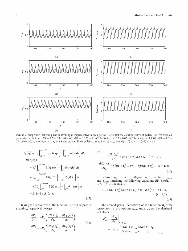