TECHNOLOGY COMPETITION AND OPTIMAL INVESTMENT TIMING: A REAL OPTIONS PERSPECTIVE

Robert J. Kauffman

Professor and Chair, Information and Decision Sciences Director, MIS Research Center Carlson School of Management

University of Minnesota, Minneapolis, MN 55455 Email: rkauffman@csom.umn.edu

Xiaotong Li

Assistant Professor of Management Information Systems Department of Accounting and MIS

University of Alabama in Huntsville, AL 35899 Email: lixi@uah.edu

Last revised: November 24, 2003

______________________________________________________________________________

ABSTRACT Companies often choose to defer irreversible investments to maintain valuable managerial flexibility in an uncertain world. For some technology-intensive projects, technology uncertainty plays a dominant role in affecting investment timing. This article analyzes the investment timing strategy for a firm that is deciding about whether to adopt one or the other of two incompatible and competing technologies. We develop a continuous-time stochastic model that aids in the determination of optimal timing for managerial adoption within the framework of real options theory. The model captures the elements of the decisionmaking process in such a way so as to provide managerial guidance in light of expectations associated with future technology competition. The results of this study suggest that a technology adopter should defer its investment until one technology’s probability to win out in the marketplace and achieve critical mass reaches a critical threshold. The optimal timing strategy for adoption that we propose can also be used in markets that are subject to positive network feedback. Although network effects usually tend to make the market equilibrium less stable and shorten the process of technology competition, we show why technology adopters may require more technology uncertainties to be resolved before widespread adoption can occur. Keywords: Capital budgeting, decision analysis, investment timing, network externalities,

option pricing, real options, stochastic processes, technology adoption. ______________________________________________________________________________ Acknowledgements: A preliminary version of this paper has been circulated at Case Western Reserve University, Duke University, INSEAD, University of Michigan, Drexel University, University of Wisconsin and the University of Minnesota. We thank John Conlon, William Lovejoy, Jim Smith, Vincent Wang and Keith Womer for their helpful suggestions and comments, and Qizhi Dai, Paul Tallon and Kevin Zhu for their input on related research on the application of the theory of real options. Rob Kauffman acknowledges the MIS Research Center for partial support.

1

I. INTRODUCTION

The recently unprecedented development of new technological innovations has yielded many

investment opportunities for firms. However, such innovations are usually associated with

significant uncertainties that derive from the nature of the technology itself, with the extent of the

consistency of investor perceptions about the quality of its solution capabilities, and from the

extent that competition is occurring in the market around similar kinds of innovations. As a

result, adopting the right technology at the right time becomes a challenging issue that many

managers must face head on, if they are to achieve effective decisionmaking on behalf of their

firms. In this study, we propose a new model based on the theory of real options that is intended

to provide senior managers with a tool to address this issue in a manner that balances effective

managerial intuition with a depth of insight that is only possible with the application of rigorous

methods. At the core of our perspective—and the theory of real options, in a larger sense—is

the idea that every successful business manager must understand the fundamental tradeoff

between risk and reward (Amram, Kulatilaka and Henderson, 1999; Balasubramian, Kulatilaka

and Storck, 1999). Recent efforts have been made to understand potential benefits associated

with real options in multiple information systems (IS) contexts, including software development

and enterprise systems module adoption (Taudes, 1998; Taudes, et al., 2000), banking IT

infrastructures (Panayi and Trigeorgis, 1998), software development project portfolios (Bardhan

et al., 2004), and decision support systems (Kumar, 1999). All these papers, however, deal with

investment evaluation problems in the absence of technology competition.

A. Investment Decisions for Competing Technologies

Very often, however, senior managers must consider whether and when to adopt one of two

incompatible competing technologies. Leading examples in our time include Sun

2

Microsystems’ Java and J2EE software development environment versus the Visual Basic,

Visual Studio and .Net development environments of Microsoft. In addition, there are many

cases of intra-technology competition in which somewhat different, and somewhat compatible

technologies compete within a technology standard (Besen and Farrell 1994), increasing the

anxiety of the marketplace as to how fast the marketplace will shift to embrace the new

technological innovations. We need look no farther than recent developments around the IEEE

standards for Wi-Fi fixed location wireless computing. Although many hardware and software

vendors have been working to create compliant products for the 802.11b standard, the market has

recently been shaken up by indications that the 802.11g standard offers faster throughput and

greater effective range.

A typical technology investment project requires a significant initial outlay of capital and is

generally either partially or wholly irreversible. In addition, technology investment projects

usually bear significant business and technological uncertainties, especially in terms of the

variance of future cash flows. Moreover, it is typical that some of the uncertainties will be

resolved as time passes, changing future period expected values to future period realized values.

The “surprise value” of this information that is revealed to a decisionmaker in the future has the

potential to change the perceived value of a project and to shift the sentiments that senior

managers express about willingness to invest (Dos Santos, 1991).

B. Real Options and Technology Adoption

This is the essence of “option value.” The characteristics that we have just described—risk

expressed in variance terms, and the value of new information—make the financial economic

theory of real options an appropriate theoretical perspective for evaluating technology

investment projects under uncertainty and risk (Benaroch, 2002). The theory offers a number of

3

useful modeling and analysis tools that are uniquely suited for this purpose. For decades,

researchers in financial economics and strategic management have recognized that option pricing

theory had the potential to be applied to real assets and organizational investments in property,

plants and other capital equipment (Myers, 1977; Mason and Merton, 1985; Kulatilaka and

Marks, 1988). Other authors have more recently written that the theory of real options has the

potential to play a role in the assessment of technology investments, business strategies and

strategic alliances in the highly uncertain and technology-driven digital economy (Kumar, 1996;

Benaroch and Kauffman, 1999 and 2000). Unlike other standard and tried-and-true methods for

evaluating corporate resource allocation decisions, the theory of real options, and the

methodologies that implement it acknowledge the importance of managerial flexibility and

strategic adaptability in settings that involve technology investment. Although some authors

have written about some of the shortcomings of applying real option investment evaluation

methods (Tallon et al., 2002), its advantages over other capital budgeting methods (like static

discounted cash flow or DCF analysis) have been widely recognized for the analysis of strategic

investment decisions under uncertainty (Amram and Kulatilaka,1999; Luehrman, 1998a and

1998b; Trigeorgis, 1997).

Although option pricing theory has been extended beyond the evaluation of financial

instruments, and the overall mode of thinking that the theory involves matches senior

management needs for technology evaluation, it is important that we caution the reader to

recognize that there are some technical issues lurking just below the surface of the intuition that

deserve our comment. First, option pricing theory is founded on the market tradability of the

asset on which the option has been created. Unfortunately though, most knowledgeable

observers and option pricing theorists will surely point out that technology investment projects

4

are not subject to the valuation of the market. Moreover, technology projects are often specific

assets for the firms that invest in them, and as a result, it is unlikely that another identical project

would ever be available in the market on which to base a comparison. In financial economics

terms—and to comply with the requirements of the underlying theory—senior managers who

wish to find a traded portfolio that can completely duplicate the risk characteristics of the

underlying non-traded asset are likely to be frustrated. Without this twin security, as it is often

referred to in the literature, risk-neutral valuation is difficult to justify (Smith and McCardle,

1998 and 1999). The result is that the standard “methods toolkit” for option pricing may be

inappropriate to apply.

Second, the business value of a potential investment project is assumed to follow a

symmetric stochastic process. The stochastic process that is most commonly used in real option

analysis is geometric Brownian motion, as illustrated by McDonald and Siegel (1986). But

models that incorporate the Brownian geometric motion stochastic process assume that there are

no competitive impacts on the cash flows and future payoffs of the project. The essence of the

concern is the possibility of competition affecting a technology project investment’s future cash

flows. Why? Because competition is likely to cause the distribution of future project values to

become asymmetric: higher project values are less likely to occur because of the potential

competitive erosion of value.

As Kulatilaka and Perotti (1998) and other business innovators have pointed out, the benefits

of early preemptive investment may strategically dominate the benefits of waiting when the

competition is very intense. These problems associated with traditional real option modeling

motivate us to model technology investments from a new perspective. Instead of stochastically

modeling the investment project value—as might be the case for traditional assessment of

5

technology projects using the real option methods—our insight is that the standard Brownian

motion assumption can be used directly model the technology competition process.

C. The Process View of Technology Competition

To effectively make our general argument about the appropriateness of representing the

competitive process that occurs around a technology investment project, it is important that we

first bring into clearer focus what we mean by the “typical process” of technology competition.

We note four basic elements of the process of technology competition that may affect the real

option valuation of technology investment projects. They include:

Problem identification. An important business problem that the firm faces is identified

and new technology solutions are sought to solve it.

Proposed technology solutions. Technology developers and vendors make proposals to

the firm for different approaches that they believe will solve the problem.

Solution testing and comparison. The firm observes different technologies competing in

the market and managers evaluate and test their effectiveness and draw conclusions based

on the appropriate comparisons.

Technology standardization. Over time, the marketplace will reveal which technology or

technology solution is the best. As a result, one can expect to see the application of the

technology to solve the problem to become increasingly standardized.

When a company plans a technology investment when a two-technology standards battle is

present, it usually faces two questions. Which technology is likely to eventually win the

standards battle? How long will it take for the technology competition process to end? In this

paper, we will show why the answers to these two related questions play important roles in a

firm’s technology investment decisionmaking. More specifically, our model suggests that a firm

6

should defer technology adoption and let some of the relevant uncertainties in the world be

resolved before the technology competition process reaches an investment viability threshold.

We will shortly lay out the characteristics of this threshold. The managerial guidance that we

offer is that firm should adopt a technology immediately if the current state of technology

competition reaches this threshold. We also consider the drivers of competition that affect the

market’s ability to permit this threshold to be reached.

Although our greater focus is on the competition between incompatible technologies, we also

address the more general issue of compatibility in this paper. We will demonstrate how

significant switching costs and possible technology lock-in may give technology adopters the

incentive to wait. Our approach to understanding this problem is especially accommodating of

scenarios under which strong network effects exist. It turns out, based on our modeling efforts to

develop this theory, that strong network feedback has the potential to shorten the technology

competition process by increasing the observed volatility of adopter preferences. The reason

why technology adopters usually will act much more quickly in the presence of strong network

externalities is not because that they can tolerate the greater uncertainty. Instead, the self-

reinforcing network feedback effects make technology adopters’ expectations reach the optimal

threshold more quickly.

D. Plan of the Paper

The rest of this paper is structured to communicate the analysis details of the story behind

this theory-based interpretation, and to provide an effective basis for the acceptance of the ways

that we will use the theory of real options to create a new evaluative methodology. In Section 2,

we begin with a formal presentation of an option-based investment timing model and show how

we reach a closed-form analytical solution. In Section 3, we show the linear relationship

7

between investors’ expectations and the optimal timing solution generated by our investment

viability model. We also explore the roles of technology switching costs and network effects in

affecting technology investors’ decisions. In Section 4, we present the results of numerical

analyses and simulations that are aimed at showing the robustness of the modeling approach that

we propose to determine when a firm should adopt a technology that is in the midst of a

standards battle. Section 5 concludes the paper with a discussion of the primary findings and

some consideration of the next steps in developing this stream of research.

II. A REAL OPTIONS MODEL FOR ADOPTING OF COMPETING TECHNOLOGIES

In this section of the paper, we discuss the setup of an option valuation model for the

adoption of competing technologies. The model is designed to capture the technology

competition that leads to an established technological standard as a stochastic process, whose

drift over time presents technology evaluation issues that can be addressed via the specification

of a real option pricing model. Our modeling choices permit us to assess the appropriate timing

for adoption, based on the use of a ratio metric that helps a firm to know whether it has reached a

threshold beyond which investment deferral no longer makes sense. (For ease of reading our

modeling development, the modeling notation and construct definitions are included in Table 1.)

A. Modeling Preliminaries

Consider a risk-neutral firm that faces a technology investment opportunity. Setting aside the

potential outcome of technology competition for a moment, we will assume that the expected

payoff of the technology investment project is a positive constant V as of the time the technology

investment is made. To implement the technology project, the firm must adopt one of two

competing technologies, called Technology S1 and Technology S2. We use standard Brownian

motion, w(t), with dw = σdz, to characterize the dynamics of competition between Technology S1

8

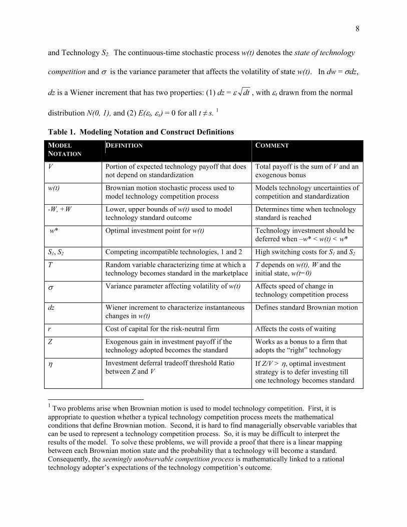
and Technology S2. The continuous-time stochastic process w(t) denotes the state of technology

competition and σ is the variance parameter that affects the volatility of state w(t). In dw = σdz,

dz is a Wiener increment that has two properties: (1) dz = ε dt , with εt drawn from the normal

distribution N(0, 1), and (2) E(εt, εs) = 0 for all t ≠ s. 1

Table 1. Modeling Notation and Construct Definitions MODEL NOTATION

DEFINITION COMMENT

V Portion of expected technology payoff that does not depend on standardization

Total payoff is the sum of V and an exogenous bonus

w(t) Brownian motion stochastic process used to model technology competition process

Models technology uncertainties of competition and standardization

-W, +W Lower, upper bounds of w(t) used to model technology standard outcome

Determines time when technology standard is reached

w* Optimal investment point for w(t) Technology investment should be deferred when –w* < w(t) < w*

S1, S2 Competing incompatible technologies, 1 and 2 High switching costs for S1 and S2

T Random variable characterizing time at which a technology becomes standard in the marketplace

T depends on w(t), W and the initial state, w(t=0)

σ Variance parameter affecting volatility of w(t) Affects speed of change in technology competition process

dz Wiener increment to characterize instantaneous changes in w(t)

Defines standard Brownian motion

r Cost of capital for the risk-neutral firm Affects the costs of waiting

Z Exogenous gain in investment payoff if the technology adopted becomes the standard

Works as a bonus to a firm that adopts the “right” technology

η Investment deferral tradeoff threshold Ratio between Z and V

If Z/V > η, optimal investment strategy is to defer investing till one technology becomes standard

1 Two problems arise when Brownian motion is used to model technology competition. First, it is appropriate to question whether a typical technology competition process meets the mathematical conditions that define Brownian motion. Second, it is hard to find managerially observable variables that can be used to represent a technology competition process. So, it is may be difficult to interpret the results of the model. To solve these problems, we will provide a proof that there is a linear mapping between each Brownian motion state and the probability that a technology will become a standard. Consequently, the seemingly unobservable competition process is mathematically linked to a rational technology adopter’s expectations of the technology competition’s outcome.

9

In many continuous-time real options models (e.g., McDonald and Siegel, 1986; Bernardo

and Chowdhry, 2002), deterministic drift parameters are included, in addition to the stochastic

parameter. However, only the stochastic parameter is needed in our model. More importantly,

the martingale property of standard Brownian motion allows us to establish a linear mapping

between w(t) and the firm’s expectations of the technology competition outcome. The

martingale property is well known in financial economics in terms of current stock prices being

informationally efficient, and thus being the best estimator for future stock prices (LeRoy, 1989).

After a random time T, one of the two technologies, S1 and S2, will prevail and become the

standard solution. To model the time T at which the standard emerges, we use an upper

boundary +W and a lower boundary, –W, with –W < w(t=0) < +W. The technology competition

will finish and one technology will emerge as the standard solution when the stochastic

technology competition, w(t), reaches either +W or –W. If the stochastic process, w(t), reaches

+W first, then Technology S1 will dominate Technology S2 to become the standard technology at

time T. The result will be opposite if w(t) reaches –W first. So an increase in w(t) will make

Technology S1 more likely to prevail in the market and a decrease in w(t) will make Technology

S1 less likely beat Technology S2 in the competition.

The approach that we use to determine the uncertain technology standardization time T is

similar to the modeling technique used in Black and Cox (1976), Leland (1994) and Grenadier

and Weiss (1997). The outcomes of the technology competition will affect the payoff of a

technology investment project that adopts either Technology S1 or Technology S2. To quantify

this, we assume that there is an exogenous gain in investment payoff, Z, at time T if the

technology adopted becomes the standard. If the solution adopted fails in the competition, then

the value gain will be 0. We also can assume that there is an exogenous value loss in this case.

10

But this assumption will not enhance the generality of our model since we can easily adjust V to

normalize this value loss to 0. It may be more helpful for the reader to think of Z as a bonus for

adopting the “right” technology. The reader should also note that we assume that the switching

costs between the two incompatible technologies are prohibitively high. This technology lock-in

situation gives the firm little flexibility to switch once it has adopted one technology.

Let the cost of capital for the technology investment project be r > 0. Since we assumed that

V is constant over time, the firm’s technology investment strategy is very simple if no

consideration is given to the effect of technology competition between S1 and S2. The firm

should invest immediately if V ≥ 0, and never invest otherwise. However, the decisionmaking

problem becomes more complicated when we consider the competitive dynamics that may occur

between Technology S1 and Technology S2. The expected total payoff from the technology

investment with technology competition may be greater than the baseline expected payoff V.

Why? Because the firm can gain Z if the technology solution it adopts wins the standards race at

time T. More importantly—and a factor that makes the theory of real options especially relevant

for our analysis—is that it may be valuable to defer the investment to resolve the uncertainty

surrounding the two competing technologies.

To derive the firm’s optimal investment strategy, it is necessary to quantify the value of the

options that are embedded in the technology investment opportunity. Before committing to the

investment, the firm has an option to choose one of the two competing technologies. When it

decides to invest, the firm exercises its adoption option, selecting the technology that it believes

to be more promising. The expected investment payoff can be derived by dynamic optimization.

Let F(w) denote the expected value gain through the standardization bonus Z if the company

decides to invest, where w is the state of technology competition. So the expected investment

11

payoff at w(t) is V+F(w). Note that the company can adopt either S1 or S2 at the time of the

investment. Let F1(w) and F2(w) denote the expected value gain if the company decides to adopt

S1 and S2 at w, respectively. For a rational risk-neutral company that always maximizes its

expected investment payoff, we know F(w)=Max[F1(w), F2(w)]. So, to calculate the expected

investment payoff, we need to derive values for F1(w) and F2(w).

We first derive F1(w). F2(w) then can be found in a similar way. Since F1(w) generates no

interim cash flows when w is between –W and +W, Bellman’s principle suggests that the

instantaneous return on F1(w) should be equal to its expected capital gain. So F1(w) must satisfy

the equilibrium equation rF1dt = E(dF1).

Expanding dF1 using Ito’s Lemma 2 yields 2''11 ))((

21 dwwFdF = . By plugging dw = σdz into

this equation, we obtain 2''1

21 ))((

21 dzwFdF σ= . Now, since , we can

rewrite the equilibrium equation, rF

dtdtEdzE == )(])[( 22 ε

1dt = E(dF1), as dtwFdt )(''11 = dzEwF2

])[()(2

22''

1

2 σσ=rF or

simply 0)(21

1''

12 =− rFwFσ .

In addition, F1(w) must satisfy two boundary conditions at w = -W and w =+ W: f1(+W) = Z

and f2(-W)=0. The first boundary condition says that the firm that adopts Technology S1 will

gain payoff Z when the state of technology competition, w, reaches +W first. But if the state of

technology, w, reaches –W first, then the firm will gain nothing. So the solution to this second

2 Ito’s Lemma is a well known theorem in stochastic calculus that is used to take derivatives of a stochastic process. Its primary result is that the second order differential terms of a Wiener process become deterministic when they are integrated over time. The interested reader should see Merton (1990) for additional details.

12

order differential equation is σσrwrw

BeAewF22

1 )(−

+= where 01

232

>

−=

−−

σσrWrW

eeZA

and 01

232

<

−=

−−

σσrWrW

eeZB . For F2(w), the solution will also satisfy the Bellman

equilibrium equation, but the two boundary conditions are 0)(2 =WF and . The

solution is

ZWF =− )(2

.)(22

2σσ

rwrw

AeBewF−

+= Since F1(w) is monotonically increasing in w and

F1(w)= F2(-w), we can prove that

≤+

≤+=

−

−

)(2

2

AeBe

wBeAewF

wrw

wrw

σ

σ

< 0w

W

−

≤02

2

Wfor

forr

r

σ

σ

Since we know the expected investment payoff at the time of investment, we are able to find

the optimal timing to make the investment. There are both benefits and costs associated with the

option to defer the investment. Waiting will erode the expected investment payoff V in terms of

its present value at time 0. However, waiting longer will resolve more uncertainties about the

competition between Technology S1 and Technology S2.

Consider two extreme cases. In the first one, the firm invests at time 0. So it will maximize

the present value of V but faces uncertainties in the technology competition. In the other, the

firm waits until one of the two competing technologies becomes the standard. At that time, the

firm’s expected investment payoff will be V + Z, but the waiting time also will erode this

composite payoff in terms of its present value at time 0. Therefore, the optimal investment

timing strategy must balance the benefits and costs associated with investment deferral. One

may guess that a firm will invest at some thresholds of w(t). We prove this in the next theorem.

□ THEOREM 1 (THE OPTIMAL INVESTMENT TIMING STRATEGY THEOREM). There are two thresholds w* and –w*, where w*∈ [0, +W]. Given w∈ [-W, +W], the firm will invest immediately if w is outside of [-w*, +w*]. Otherwise, it will defer the investment

13

until w(t) reaches either +w* or -w*. If w(t) reaches +w* first, the firm will adopt Technology S1. If w(t) reaches –w* first, it will adopt Technology S2.

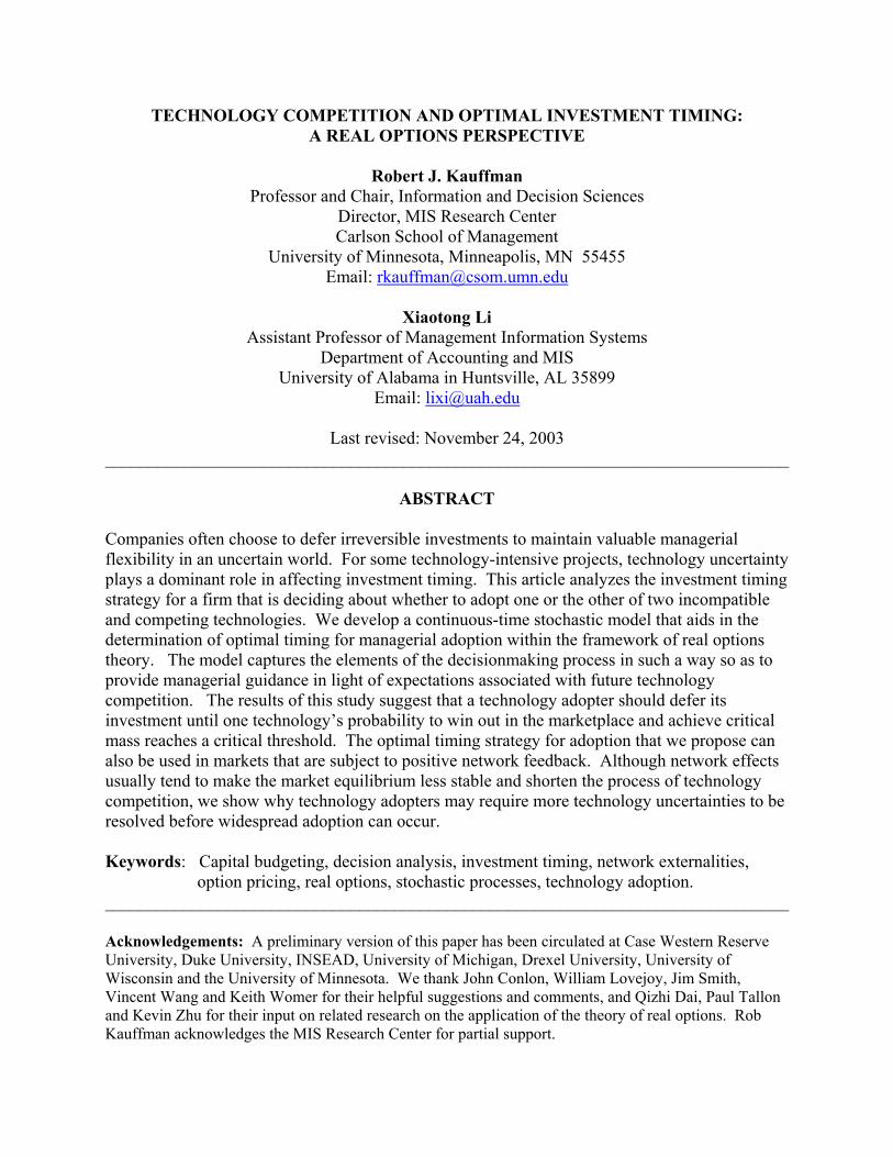
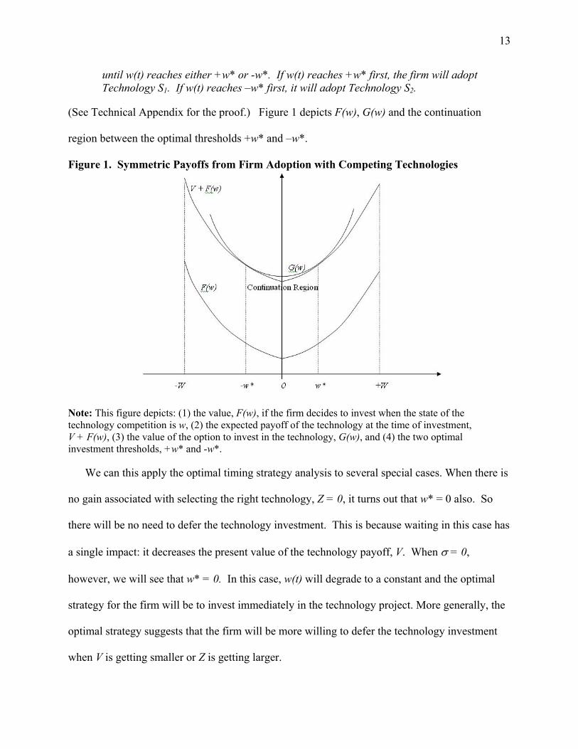
(See Technical Appendix for the proof.) Figure 1 depicts F(w), G(w) and the continuation

region between the optimal thresholds +w* and –w*.

Figure 1. Symmetric Payoffs from Firm Adoption with Competing Technologies

Note: This figure depicts: (1) the value, F(w), if the firm decides to invest when the state of the technology competition is w, (2) the expected payoff of the technology at the time of investment, V + F(w), (3) the value of the option to invest in the technology, G(w), and (4) the two optimal investment thresholds, +w* and -w*.

We can this apply the optimal timing strategy analysis to several special cases. When there is

no gain associated with selecting the right technology, Z = 0, it turns out that w* = 0 also. So

there will be no need to defer the technology investment. This is because waiting in this case has

a single impact: it decreases the present value of the technology payoff, V. When σ = 0,

however, we will see that w* = 0. In this case, w(t) will degrade to a constant and the optimal

strategy for the firm will be to invest immediately in the technology project. More generally, the

optimal strategy suggests that the firm will be more willing to defer the technology investment

when V is getting smaller or Z is getting larger.

14

We find that there is a critical ratio between Z and V in Proposition 1 that can guide

investment decisionmaking. The firm will defer the technology investment until w(t) reaches

+W or –W when Z/V is greater than or equal to the critical ratio.

□ PROPOSITION 1 (THE INVESTMENT DEFERRAL TRADEOFF THRESHOLD RATIO PROPOSITION). There is a critical ratio, the investment deferral tradeoff threshold ratio η, between Z and V. If the ratio Z/V is greater than or equal to η, the optimal investment timing strategy is to defer the investment until one technology becomes the standard. Moreover, the optimal timing solution w* depends only on Z/V, and not on the separate values of either V or Z.

See the proof in the Technical Appendix.

The Investment Deferral Tradeoff Threshold Ratio Proposition suggests that the adopting

firm’s optimal investment strategy is to defer the investment until all of the relevant uncertainties

associated with technology competition are resolved if Z/V ≥ η. In other words, the firm should

defer the investment until one technology becomes the standard, if the outcome of the standards

battle appears likely to have a significant impact on the technology investment’s expected

payoff. This proposition also says that the actual values of V or Z are irrelevant to the timing

decision as long as we know the ratio between Z and V, which is intuitively plausible.

For the optimal investment thresholds found in our model, it is important to show how they

are affected by the model parameters. Because of the symmetry of our model, we only need to

conduct a comparative static analysis on the positive threshold w*. This leads to Proposition 2:

□ PROPOSITION 2 (THE COMPARATIVE STATICS PROPOSITION). For a positive investment threshold w*∈ (0, W), the following comparative static results must hold:

.0*,0*,0*,0*,0*<

∂∂

>∂∂

<∂∂

<∂∂

>∂∂

Wwand

Zw

Vw

rww

σ

See the Technical Appendix for the proof.

The results of the comparative static analysis are readily interpreted. First, if the gain Z

from adopting the right technology is large compared to V, the firm will wish to wait for more

15

uncertainty to be resolved with respect to the technology. Second, because increases in W and

decreases in σ will tend to prolong the technology competition process, the firm will tend to

adopt sooner because the present value of Z will be smaller. Finally, increasing the discount rate

r will make waiting more costly and, as a result, the firm will tend to shorten its waiting time.

We next interpret the results of our model from another perspective and demonstrate the

significance of technology adopters’ expectations in technology investment timing.

SWITCHING COSTS, ADOPTER EXPECTATIONS AND NETWORK EFFECTS

We consider the problems of switching costs and lock-in, the role of adopter expectations,

and the role of network externalities in technology adoption decisionmaking.

A. Switching Costs and Lock-in

An assumption that we make in this model is that the switching costs between the two

technologies are very high. Although this assumption may seem restrictive at first, significant

switching costs are common in technology-intensive industries and often lead to a situation

known as technology lock-in (Farrell and Shapiro, 1989; Klemperer, 1995; Varian 2001). Based

on the comparative static results, we can relax this assumption and examine how decreases in

switching costs affect the optimal investment strategy. In our model, a decrease in switching

costs will affect two parameters. The switching costs will dwarf the uncertain exogenous value

gain, Z, because firms that have adopted the non-standard technology may later choose to switch

to the standard one at the expense of some switching costs. Also the switching costs increase the

certain investment payoff V because a part of Z becomes a certain payoff. Since the derivatives

0*<

∂∂

Vw and 0*

>∂∂

Zw , decreases in switching costs make waiting less attractive. But clearly,

technology adopters are willing to wait because they are afraid of getting locked into the non-

16

standard technology. Without proper coordination, significant switching costs may lead to

Pareto-inferior equilibria, and possibly unacceptably slow, inertial adoption. Consequently,

some technology vendors may voluntarily promote open standards or technology interoperability

to reduce switching costs and to boost potential adopters’ confidence about the future benefits

stream from the technology.

B. The Role of Expectations

As we mentioned in a brief footnote earlier in this paper, one difficulty that managers will

face in interpreting our model is that the Brownian motion process w(t) that represents the

technology competition process will be hard to define in practice. In Proposition 3, we show that

w(t) can be interpreted as the technology adopter’s expectations of the outcome of the technology

competition.

□ PROPOSITION 3 (THE EXPECTED TECHNOLOGY STANDARD PROPOSITION). At point w(t) where –W < w(t) < +W, the probability for Technology S1 to defeat Technology S2 and to become the future standard is given by P1 = (W+ w(t))/2W. At the same poin in timet, the probability for Technology S2 to defeat Technology S1 and to become the future standard is given by P2 = 1- P1 = (W- w(t))/2W.

The proof is omitted. 3

With knowledge of the relationship between w(t) and the firm’s expectations, we are able to

provide a more precise interpretation of the Optimal Investment Timing Strategy Theorem. The

optimal timing strategy for the risk-neural firm is to defer the technology investment until it

expects that either Technology S1 or Technology S2 will win the competition with a probability

of (W+w*)/2W. Rational decisionmakers will always adopt the technology that is expected to

have a higher probability to win. So if w(t) hits w* first, Technology S1 is expected to win the

3 The proposition directly follows from the fact that w(t) is a martingale. For more details about the hitting probabilities of a martingale upon which the proof is based, we refer the interested reader to Durrett (1984).

17

competition with a probability of (W+w*)/2W > ½ . But if w(t) hits -w* first, Technology S2

ought to win with a probability of (W+w*)/2W. Note that P1 and P2 only depend on σ/W, and

not on the separate values of either W or σ. This interpretation clearly indicates that the

technology adopter’s expectations of future technology competition outcomes play a crucial role

in its investment timing decision.

As far as the technology vendors are concerned, their abilities to effectively manage their

potential customers’ expectations are also critical. A commonly used strategy in technology

competition is penetration pricing, where one technology vendor unilaterally and aggressively

cuts prices to gain market share or preempt its competitors at an early stage in the technology

competition. This strategy not only makes a firm’s technology more attractive because of the

lower price. The vendor also affects other potential adopters’ expectations by showing its own

determination to win the standards battle. A similar strategy is survival pricing, where a weak

competitor cuts its product’s price defensively to escape a defeat in a standard battle. A survival

strategy is hard to make work, according to Shapiro and Varian (1999), because it signals the

player’s weakness.

Under the scenario presented in our model, we can treat the signaling effect as an exogenous

shock to the expectations of potential technology adopters. The negative impact on expectations

may totally offset or even surpass the positive effects brought on by competitive pricing. In a

general equilibrium model, the results of our model can be related to many other interesting

issues of expectations management in technology competition.

C. Technology Competition with Network Effects

We use a continuous-time Brownian motion to directly model a technology adopter’s

expectations that also continuously change. Although we have proved that expectations are

18

linear in w(t), there is another question that we have not yet fully addressed. Is it appropriate to

assume that the adopter’s expectations can be characterized by Brownian motion? As long as the

adopter’s expectations are rational and consistent, the martingale property of w(t) is justified by

the law of iterated expectations. 4 In addition, since only unpredictable new information can

change the adopter’s expectations, w(t) should have a memoryless property.

However, if we use w(t) to model some directly observable variables like each technology’s

market share, these two properties are actually much harder to justify. 5 One reason is that many

technology competition processes are subject to positive network feedback that makes a strong

technology grow stronger (Katz and Shapiro, 1994; Kauffman et al., 2000; Brynjolfsson and

Kemerer, 1996). Network effects stem from the efficiencies associated with a user base for

compatible products. Consequently, the technology with a larger market share can be expected

to gain more market share from its competitor in our model. But note that this directly violates

the martingale property and can result in dependent increments (in lieu of memoryless

increments) of the market share. Although network effects do not undermine our modeling

assumptions since we directly model adopter’ expectations, their relationships with our model

nevertheless should not be ignored.

In our model, network effects affect the technology adoption dynamics through two

channels: through the technology adopter and through the market. The externalities created by

4 The law of iterated expectations states that today’s expectation of what will be expected tomorrow for some variable in a latter period, is simply today’s expectation for the variable’s value in the latter period. For additional details, the reader should see Walpole et al. (2002). 5 Issues of this sort frequently arise in the midst of efforts to bring a theoretical perspective into more practical uses for analysis and evaluation. The reader should recognize this as inevitable, just as the application of agency theory for contract formation and managerial incentives development (Austin, 2001; Banker and Kemerer, 1992) or the theory of incomplete contracts for interorganizational IS investments and governance (Bakos and Nault, 1997; Han, Kauffman and Nault, 2004) is founded on relatively strict assumptions. In spite of this, the theoretical perspectives and the modeling approaches that complement them still offer rich and meaningful managerial insights.

19

network effects usually make it more beneficial to adopt the winning technology. In our model,

the investment threshold ratio η = Z/V can become larger due to strong network effects. As a

result, the optimal timing threshold, w*, will increase. According to our comparative static

results, the technology adopter will require more certainty about the outcome of the standards

battle before making an investment decision. This effect requires that the technology adopter be

more patient and wait longer to let more uncertainties in the market be resolved.

But strong network effects usually also result in “tippy” markets that can significantly

shorten the technology competition process. In markets subject to strong network externalities,

any market equilibrium will be highly unstable and the expected winning technology may be

able to obtain a commanding market share even in a very short period of time (Farrell and

Klemperer, 2001; Farrell and Katz, 2001). We have recently seen this occur with some of the

new wireless technologies and instant messaging services (Kauffman and Li, 2003). So network

effects can reduce the expected duration of the technology competition process in our model by

increasing the volatility of w(t). This will occur because the expectation of the random variable

representing the time at which a technology becomes standard in the marketplace, T,

monotonically decreases in σ.

To sum up, our model suggests that network externalities either cause a delay or expedite

technology adoption, but this depends on adopter and market-related factors. In general, strong

network effects tend to result in very fast adoption of the technology that adopters believe will be

most likely to win the standards competition. In some cases, however, network externalities will

make people adopt a technology too early, even though waiting is Pareto-preferred (Choi and

Thum, 1998; Au and Kauffman, 2001). A final point suggested by our model is that technology

adopters actually require more assurance about the future technology standard outcome when

20

they make technology investment decisions, although network effects usually speed up their

decisions to adopt.

SIMULATION, NUMERICAL EXPERIMENTS AND INTERPRETATION

This section discusses a firm-level decisionmaking simulation for technology adoption in the

presence of a standards battle between two technologies.

A. Simulation Setup and Outcome

Entry Conditions. We assume that the investment decision will be irreversible. Once it is

made, the firm will be locked into the costs and benefits stream associated with the adopted

technology. Our goal is to determine the firm’s optimal technology adoption timing strategy,

w*. To initiate this simulation, we require that the decisionmaker who is contemplating

adopting the technology at the firm will know the following information:

□ The decisionmaker’s current expectations of each technology’s probability to win the

standards battle will determine w(t=0), the initial state of technology competition.

□ The decisionmaker’s current estimate of the duration of the technology competition

process will determine the appropriate values of W and σ .

□ The decisionmaker should be able to make a reasonable estimate of Z/V, the ratio

between the bonus for adopting the technology that becomes the standards battle winner,

and the firm’s baseline payoff from investing in the technology project, regardless of the

technology choice.

□ The decisionmaker should know the discount rate r that affects the costs of waiting.

We normalize V and W to 1 for the numerical analysis. The discount rate r is assumed to be

10%. The likelihood that either technology will become the standard is 0.50, from which follows

that w = 0 at time 0. The firm also expects that one of the two technologies will emerge as the

21

winner in four years. This assumption causes the numerical value of the standard deviation, σ, to

be around 0.50. We also set the value of Z, the exogenous gain in business value if the

technology becomes a standard, at 0.5V.

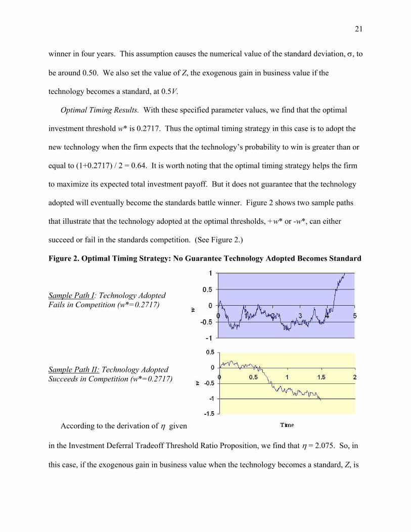
Optimal Timing Results. With these specified parameter values, we find that the optimal

investment threshold w* is 0.2717. Thus the optimal timing strategy in this case is to adopt the

new technology when the firm expects that the technology’s probability to win is greater than or

equal to (1+0.2717) / 2 = 0.64. It is worth noting that the optimal timing strategy helps the firm

to maximize its expected total investment payoff. But it does not guarantee that the technology

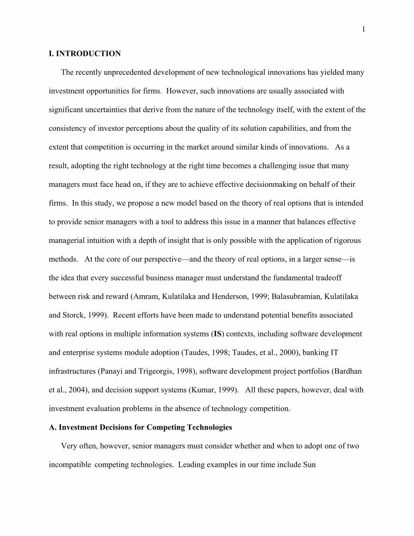
adopted will eventually become the standards battle winner. Figure 2 shows two sample paths

that illustrate that the technology adopted at the optimal thresholds, +w* or -w*, can either

succeed or fail in the standards competition. (See Figure 2.)

Figure 2. Optimal Timing Strategy: No Guarantee Technology Adopted Becomes Standard Sample Path I: Technology Adopted Fails in Competition (w*=0.2717)

Sample Path II: Technology Adopted Succeeds in Competition (w*=0.2717)

According to the derivation of η iven

d, Z, is

g

in the Investment Deferral Tradeoff Threshold Ratio Proposition, we find that η = 2.075. So, in

this case, if the exogenous gain in business value when the technology becomes a standar

22

larger than 2.075V. The result is that the optimal investment strategy is to wait until one

technology emerges as the winner.

B. Model Robustness

We also use computer simulation to obtain some Monte Carlo results. Because a closed form

solution is given in our model, the primary goal of computer simulation is to test its robustness

rather than generating numeric solutions. We use ANSI C to code the simulation. With 0.03 as

an increment in w, we draw the 100,000 sample average investment payoffs as a function of w in

Figure 3. We set the number of sample paths used in our simulation sufficiently large to make

sure that these sample average payoffs are very close to the expected investment payoffs.

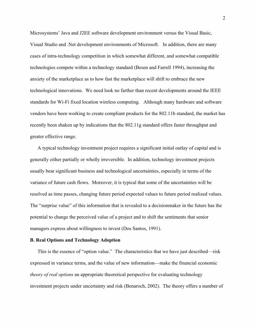
Figure 3a is a benchmark simulation where no parameter noise has been introduced. It shows

that the sample average payoff function achieve its maximum at w = 0.27, which is very close to

the closed-form solution w* = 0.2717, given that the increment in w is 0.03 in the simulation.

Figure 3b shows the average sample payoffs when Z is uniformly distributed between 0 and 1.

Again, the payoff function achieves its maximum at w = 0.27. We let Z and σ both be uniformly

distributed and draw the sample average payoff function in Figure 3c. Here we let σ be

randomly drawn between 0.4 and 0.6: so the expected duration of technology competition could

range from 2.8 years to 6.3 years in our simulation. We intentionally set this wide range to test

the limits of our model’s robustness. The payoff curve reaches its peak at w = 2.4. The second

highest payoff is reached at w = 2.7; it is only 0.017% less than the highest payoff.

Why do we test the robustness of our model by adding random noise to the parameter space?

In the real business world, managers can not know the precise values of those parameters used in

23

Figure 3. 100,000 Sample Average Investment Payoff as a Function of w.

a) Benchmark simulation when no parameter noise is introduced. Average Payoff Reaches Maximum at w = 0.27

1.041.061.081.1

1.121.141.161.181.2

1.22

0 0.2 0.4 0.6 0.8 1 1.2

w

Ave

rage

Pay

off

b) Simulation result when Z is uniformly distributed within [0,1].

Average Payoff Reaches Maximum at w = 0.27

1.021.041.061.081.1

1.121.141.161.181.2

1.22

0 0.2 0.4 0.6 0.8 1 1.2

w

Ave

rage

Pay

off

c) Simulation result when Z is uniformly distributed within [0,1] and σ is uniformly distributed within [0.4, 0.6].

Average Payoff Reaches Maximum at w = 0.24

1

1.05

1.1

1.15

1.2

1.25

0 0.2 0.4 0.6 0.8 1 1.2

w

Ave

rage

Pay

off

24

our model. Instead, they can only use some reasonable estimates based upon available data and

their experience. So we try to demonstrate the robustness of our closed-form solution in

numerical experiments to increase managers’ confidence in adopting our model even when the

environment is noisy. Based upon these simulations, we believe that our model is very robust to

random noise in the model parameter space. Like many other continuous objective functions, the

average investment payoff function in our model is very flat near the optimal point w*. This

implies that the penalty for minor deviations from the optimal strategy is small.

DISCUSSION, IMPLICATIONS AND CONCLUSION

Since the dynamics of the technology competition process play an important role in

technology adoption, we proposed a continuous-time real options model to explore this issue.

We next provide a managerial interpretation of the main findings of this research, as a basis for

assessing the usefulness of the ideas in a variety of technology competition and adoption

contexts. We also will discuss the limitations of our approach, and the agenda they prompt for

future research.

A. Interpretation and Applicability of the Main Findings

Interpretation of the Managerial Contribution. Unlike traditional real options models that

stochastically model an investment project’s value, our model uses a Brownian motion stochastic

process to simulate changes over time in a technology adopter’s expectations. This modeling

approach enjoys several distinctive advantages. First, decisionmakers’ expectations are

continuously changing in the presence of new information from the environment in which

decisionmaking occurs. Unfortunately, multi-stage discrete-time models usually cannot

accommodate this feature of the decisionmaking process. Second, the information that arrives

typically does so in random fashion. But so long as managerial expectations are rational and

25

consistent, the memoryless and martingale properties of the stochastic process that we discussed

turn out to be not too hard to justify. So, in spite of some initial concerns that we pointed out, we

believe that our use of the standard Brownian motion representation is a suitable modeling tool.

Third, many observers believe that that managerial decisionmakers’ expectations play a

fundamental role in many strategic decisionmaking processes. By characterizing managers’

expectations directly, and incorporating them into a decisionmaking model for competing

technologies, the modeling approach that we used in this paper may create power to analyze

other decisionmaking problems under uncertainty.

A major implication of our model is that a firm’s technology adoption decisions are directly

affected by what senior management decisionmakers expect to happen in the future. Since

waiting is usually expensive in a competitive environment, a technology adopter needs an

investment timing strategy to balance the trade-off between waiting and preemption. Our model

shows that in a partial equilibrium setting the optimal investment time can be directly expressed

as a function of the decisionmaker’s expectations about the outcome of the standards battle.

We also addressed the issues of technology switching costs and lock-in within the context of

technology investment timing. If competing technologies are more compatible or they compete

within an open standard, the technology uncertainties may be significantly reduced and firms

may become more aggressive in adopting new technologies. The major results of our model are

especially applicable to technology competition processes subject to strong network externalities.

We have argued that technology adopters’ expectations may become more volatile in a “tippy”

market, and that this is caused by positive network feedback. Consequently, waiting may be

more beneficial to adopters because the technological uncertainties will be resolved sooner due

to the increase in the volatility of expectations. The actual waiting time, as a result, may be

26

significantly shortened because the competition process itself usually ends much more quickly.

Breadth of Application. This approach to thinking about technology competition and

adoption has ready application in a number of interesting new business environments involving

IT. For example, in the domain of digital wireless phone technologies, we currently see a

proliferation of technology standards around the world. Kauffman and Techatassanasoontorn

(2004a, 2004b) report empirical results at the national level of adoption among countries

throughout the world to show that the presence of multiple wireless standards slows down

diffusion. In this context, there are problems that exist at the level of the firm, where the kind of

managerial decisionmaking issues arise that we describe in this paper. However, there is another

aspect: technology policymaking by regulators and government administrators who affect the

technology economy. In the presence of uncertainty about the outcome of technology

competition, these decisionmakers will be faced with the possibility of creating technology

adoption distortions through policymaking that lead to inefficient growth and diffusion, as the

information they tap into and their expectations blend together. The primary fear is that

inappropriate expectations, possibly amplified by the regulator’s distance from the actual process

of firm-level decisionmaking, may drive inefficient economic outcomes.

The same can be said for what may happen when firm-level decisionmakers are unable to

effectively process information about competing technologies, and end up with inappropriate

expectations about the likely outcome. Kauffman and Li (2003) argue that there is a risk of

rational herding, when decisionmakers at potential technology adopting firms misinterpret the

signals that are sent and received in the marketplace. Au and Kauffman (2003) further argue that

this is a problem of rational expectations, in which the information for technology adoption

decisionmaking is not able to be assembled all at once. Instead, decisionmakers obtain

27

impressions that are later weakened or consolidated, based on their interactions with other

potential adopters in the marketplace, as well as vendors and other third parties that may play an

important role in the outcome. They point out that the problem of gauging the potential of

competing technologies to achieve the status of de facto standard has occurred with electronic

bill payment and presentment technologies diffusion in the United States, slowing diffusion in

the absence of an acknowledged standard.

A similar problem has been occurring with the diffusion of fixed location wireless, the so-

called “Wi-Fi” technologies. But here also, we see an environment in the United States

characterized by the near simultaneous emergence in time of multiple standards (including

802.11b, 802.11a and 802.11g, etc.). The difficulties arise for manufacturers of electronics

products who wish to embed compatible wireless technologies into their products, including

handheld computers and PDAs, sound electronics, electronic shelf management technologies,

computer peripherals, and wireless routers and network equipment. They are faced with making

uncertain decisions about two aspects of the wireless standards: which ones will become widely

accepted by potential consumers of the products they make, and how long the standards will be

in use before they are supplanted by the next innovation. Although our model does not directly

address this issue of “standards stability,” the reader should recognize that the value of the real

options that an adopter possesses by making a commitment to a current version of a standard is

affected by a variety of market, vendor and technology innovation issues that are beyond the

managerial control of adopting firms. Indeed, this is generally true in many technology

adoption settings.

B. Limitations and Future Research

Limitations. We note three limitations of this research that deserve comment before we close

28

out our discussion. First, even though the underlying mathematics of the competing technologies

analysis that we present are fairly complex, the concepts that we have presented are relatively

straightforward in conceptual terms for use by senior managers. Some may argue that our first

concerns should be with the technical details of the modeling formulation—in particular ensuring

that the assumptions that go along with a standard Brownian motion stochastic process with

martingale features are precisely met. We chose a different approach though. Our goal was to

find a way to make an analogy between the technical details of the decision model and the

exigencies of its application in an appropriate managerial context. We offered a technical

argument to assuage the reader’s fears that some of our model’s assumptions are too stringent.

However, we believe that the single best way to think about our approach is in terms of the new

capabilities it opens up in support of managerial decisionmaking.

Second, although we have done some initial numerical analysis with our model to gauge its

robustness across a number of parameter values, there is a higher-level test for robustness that

our model still has not measured up to: construct robustness in various applied settings. Even

though additional analysis work is beyond the scope of the present paper, it would be appropriate

to conduct additional tests to see whether other issues involving uncertainty that affect adoption

decisionmaking can be incorporated. Several immediately come to mind. What will happen

when signals on the state of the technology relative to its becoming a standard in the market are

filtered or garbled or misread by an adopter, or are misrepresented by a technology vendor?

How can the model handle changes over the duration of the adoption period in the key

parameters, such as changed estimates of volatility, or shifting perceptions of the adoption time

line that firms face? Clearly, there is additional evaluative work to be done with respect to the

general aspects of the modeling approach that we have presented.

29

Third, we have not yet fully validated this approach with a real world test—something which

also is beyond the scope of the present paper. This is desirable because we do not yet know if

senior management decisionmakers will find it easy to work with the modeling parameters and

concepts. In prior work on the application of real options, for example, Benaroch and Kauffman

(2000) found that managers did not understand the concept of risk variances and the

distributional mechanics that represent stochastic outcomes. This puts a limitation on the

application of the methods, since senior management decisionmakers need to be able to work

within the modeling constructs of a recommended evaluation approach to represent their

understanding of the technology adoption valuation issues in an applied, real world context.

Understanding risks and variances is critical to successful use of the approach that we propose.

Future Research. In this study, we only modeled the dynamics of competition between two

technologies. However, our model can be extended to a more general scenario where the

technology competition among many technologies is modeled by a stochastic process involving

multi-dimensional Brownian motion. Since technology vendors can proactively influence

adopters’ timing decisions, another interesting direction for future research is to address the

timing issue in a general equilibrium model, to determine policies for adopting firms in a multi-

partite (i.e., with multiple vendors and adopters) competitive context.

In such a model, game theory is arguably the ideal tool, as suggested by Tallon et al. (2002)

and Zhu (1999), and the role of strategic expectations management should be the focal point.

Once vendors’ strategies become endogenous to a decisionmaking model, the information

asymmetry between technology adopters and vendors will emerge, affecting the manner in which

each approaches a decision about when to adopt and when to push toward the next standard. In

most cases, technology vendors will hold private information about their firms’ plans with the

30

technology, the schedule for releasing next generation versions, the speed of development, and

so on. As a result, informational asymmetry should be built into adopters’ expectations. As a

result, technology vendors with good credibility in the marketplace have the capacity to

successfully alter adopters’ expectations by selectively revealing relevant private information,

instead of making “vaporware” and other market preemption announcements.

Because it is impossible to give closed form solutions for many complicated real options

models, computer simulations and other computationally intensive approaches are suitable

research tools (Calistrate, Paulhus and Sick, 1999; Gamba, 2002). Although we derived a

closed-form solution in this study of competing technologies, we understand that closed-from

solutions are very difficult to derive in many other situations where real options analysis is

appropriate. Fortunately, the newly-available capabilities of computing resources make it

possible, consistent with widespread advances in methodologies for computational finance,

statistics and econometrics, to do numerical experiments and simulations that would not have

been cost-effective only a few years ago. These new computationally-intensive methods permit

us to ask new and more refined research questions involving real options valuation in important

applied settings. The answers that we are now able to obtain will help to guide senior

management decisionmaking related to technology adoption and advance the frontiers of

management science for decisionmaking under uncertainty.

31

TECHNICAL APPENDIX. MATHEMATICAL PROOFS OF KEY FINDINGS

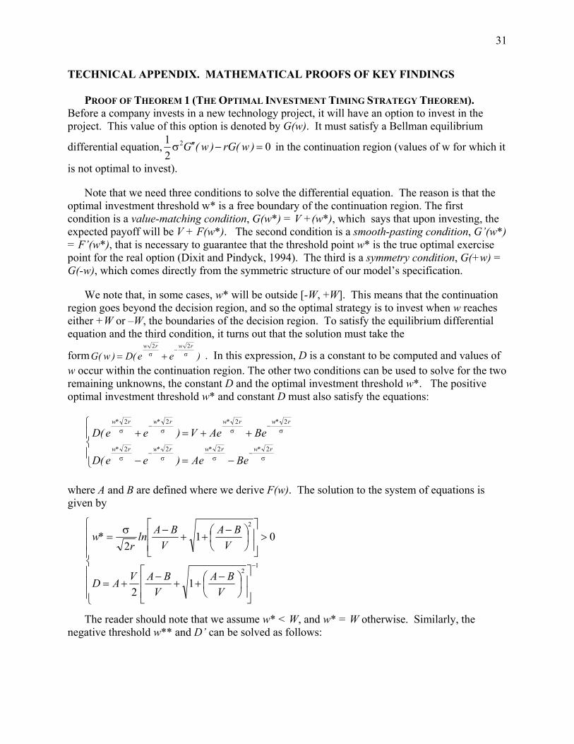
PROOF OF THEOREM 1 (THE OPTIMAL INVESTMENT TIMING STRATEGY THEOREM). Before a company invests in a new technology project, it will have an option to invest in the project. This value of this option is denoted by G(w). It must satisfy a Bellman equilibrium

differential equation, 021 2 =−′′σ )w(rG)w(G in the continuation region (values of w for which it

is not optimal to invest).

Note that we need three conditions to solve the differential equation. The reason is that the optimal investment threshold w* is a free boundary of the continuation region. The first condition is a value-matching condition, G(w*) = V +(w*), which says that upon investing, the expected payoff will be V + F(w*). The second condition is a smooth-pasting condition, G’(w*) = F’(w*), that is necessary to guarantee that the threshold point w* is the true optimal exercise point for the real option (Dixit and Pindyck, 1994). The third is a symmetry condition, G(+w) = G(-w), which comes directly from the symmetric structure of our model’s specification.

We note that, in some cases, w* will be outside [-W, +W]. This means that the continuation region goes beyond the decision region, and so the optimal strategy is to invest when w reaches either +W or –W, the boundaries of the decision region. To satisfy the equilibrium differential equation and the third condition, it turns out that the solution must take the

form )ee(D)w(rwrw

σ−

σ +=22

G . In this expression, D is a constant to be computed and values of w occur within the continuation region. The other two conditions can be used to solve for the two remaining unknowns, the constant D and the optimal investment threshold w*. The positive optimal investment threshold w* and constant D must also satisfy the equations:

−=−

++=+

σ−

σσ−

σ

σ−

σσ−

σ

r*wr*wr*wr*w

r*wr*wr*wr*w

BeAe)ee(D

BeAeV)ee(D2222

2222

where A and B are defined where we derive F(w). The solution to the system of equations is given by

−

++−

+=

>

−

++−σ

=

−12

2

12

012

VBA

VBAVAD

VBA

VBAln

r*w

The reader should note that we assume w* < W, and w* = W otherwise. Similarly, the negative threshold w** and D’ can be solved as follows:

32

=

<−=

−

++−σ

=

D'D

*wV

ABV

ABlnr

**w 012

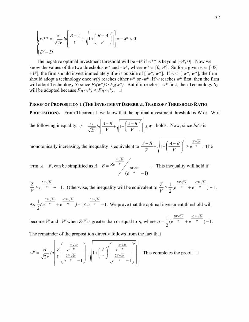
2

The negative optimal investment threshold will be –W if w** is beyond [-W, 0]. Now we know the values of the two thresholds w* and –w*, where w* ∈ [0, W]. So for a given w ∈ [-W, +W], the firm should invest immediately if w is outside of [-w*, w*]. If w ∈ [-w*, w*], the firm should adopt a technology once w(t) reaches either w* or -w*. If w reaches w* first, then the firm will adopt Technology S1 since F1(w*) > F2(w*). But if it reaches –w* first, then Technology S2 will be adopted because F1(-w*) < F2(-w*). ٱ

PROOF OF PROPOSITION 1 (THE INVESTMENT DEFERRAL TRADEOFF THRESHOLD RATIO

PROPOSITION). From Theorem 1, we know that the optimal investment threshold is W or –W if

the following inequality, WV

BAV

BAlnr

*w ≥

−

++−σ

=2

12

, holds. Now, since ln(.) is

monotonically increasing, the inequality is equivalent to σ≥

−

++− rW

eV

BAV

BA 22

1 . The

term, A – B, can be simplified as)1(

22

2

−=−

σ

σrW

rW

e

ZeBA . This inequality will hold if

122

−≥ σrW

eVZ . Otherwise, the inequality will be equivalent to 1)(

21 2222

−+≥−

σσrWrW

eeVZ .

As 1121 222222

−≤−+ σσ−

σrWrWrW

e)ee( . We prove that the optimal investment threshold will

become W and –W when Z/V is greater than or equal to η, where .1)(21 2222

−+=−

σσηrWrW

ee

The remainder of the proposition directly follows from the fact that

−

++

−

σ=

σ

σ

σ

σ

2

22

22

22

2

11

12 rW

rW

rW

rW

e

eVZ

e

eVZln

r*w . This completes the proof. ٱ

33

PROOF OF PROPOSITION 2 (THE COMPARATIVE STATICS PROPOSITION). We know that for any

w*∈ (0, +W), we have

−

++−σ

=2

12 V

BAV

BAlnr

*w . In the proof for Proposition 1, we

showed that the term, A – B, can be simplified as 1

22

2

−

=−σ

σ

rW

e

ZeBA

rW

. From this, we can prove

that 000 <∂

<∂

>∂ r

,W

,Z

and .0>σ∂

Since A – B > 0, V > 0 and

ln(.) is monotonically increasing, we can further deduce that .W

and,Z

,V

000 <∂

>∂

<∂∂

In addition, we know that 0212 >=

σ∂

∂

rr

σ

022

2 23

<σ

−=∂

σ∂

−r

rr . As a result, we can

conclude that .r

and 00 <∂

>σ∂

*w*w ∂∂ This completes the proof. ٱ

)BA( −∂−∂−∂−∂ )BA()BA()BA(

*w*w*w ∂∂

REFERENCES

Amram, M., and N. Kulatilaka (1999). Real Options: Managing Strategic Investment in an Uncertain World, Harvard Business School Press, Cambridge, MA.

Amram, M., N. Kulatilaka, and J. C. Henderson (1999). “Taking an Option on IT,” CIO Enterprise Magazine, 12, 17, 46.

Au, Y., and R. J. Kauffman (2001). “Should We Wait? Network Externalities, Compatibility and Electronic Billing Adoption,” Journal of Management Information Systems, 18, 2, 47-64.

Au, Y., and R. J. Kauffman (2003). “What Do You Know? Rational Expectations in Information Technology Adoption and Investment,” Journal of Management Information Systems, 20, 2, forthcoming.

Austin, R. D. (2001). “The Effects of Time Pressure on Quality in Software Development: An Agency Model,” Information Systems Research, 12, 2, 195-207.

Bakos, J. Y., and B. R. Nault (1997). “Ownership and Investment in Electronic Networks,”Information Systems Research, 8, 4, 321-341.

34

Balasubramian, P., N. Kulatilaka, and J. C. Storck (1999). “Managing Information Technology Investments Using a Real Options Approach,” Journal of Strategic Information Systems, 9, 39-62.

Banker, R. D. and Kemerer, C. F. (1992). “Performance Evaluation Metrics for Information Systems Development: A Principal-Agent Model,” Information Systems Research, 3, 4, 379-401.

Bardhan, I., Bagchi, S., and Sougstad, R. “Real Options Approach for Prioritization of a Portfolio of Information Technology Projects: An Illustrative Example of a Utility Company,” in R. Sprague (Ed.), Proceedings of the 37th Hawaii International Conference on Systems Science, Kona, HI, IEEE Computing Society Press, 2004. Benaroch, M. (2002) “Managing Information Technology Investment Risk: A Real Options Perspective,” Journal of Management Information Systems, 19, 2, 43-84.

Benaroch, M., and R. J. Kauffman (1999). A Case for Using Real Options Pricing Analysis to Evaluate Information Technology Project Investment," Information Systems Research, 10, 1, 70-86.

Benaroch, M., and R. J. Kauffman (2000). “Justifying Electronic Banking Network Expansion Using Real Options Analysis,” MIS Quarterly, 24, 2, 197-225.

Bernardo, A., and B. Chowdhry (2002). “Resources, Real Options and Corporate Strategy,” Journal of Financial Economics, 63, 2, 211–234.

Besen, S., and J. Farrell (1994). “Choosing How to Compete: Strategies and Tactics in Standardization,” Journal of Economic Perspectives, 8, 2, 117-131.

Black, F., and J. C. Cox (1976). “Valuing Corporate Securities: Some Effects of Bond Indenture Provisions,” Journal of Finance, 31, 2, 351-367.

Brynjolfsson, E., and C. Kemerer (1996). “Network Externalities in Microcomputer Software: An Econometric Analysis of the Spreadsheet Market,” Management Science, 42, 12, 1627-1647.

Calistrate, D., Paulhus, M., and Sick, G. (1999). “Real Options for Managing Risk: Using Simulation to Characterize Gain in Value,” Working paper, Department of Mathematics, University of Calgary, Calgary, CA.

Choi, J. P., and M. Thum (1998). “Market Structure and the Timing of Technology Adoption with Network Externalities,” European Economic Review, 42, 2, 225-244.

Dixit, A., and R. Pindyck (1994). Investment Under Uncertainty, Princeton University Press, Princeton, NJ.

Dos Santos, B. L. (1991). “Justifying Investments in New Information Technologies,” Journal of Management Information Systems, 7, 4, 71-90.

Durrett, R. (1984). Brownian Motion and Martingales in Analysis, Wadsworth Publishing, Belmont, CA.

Farrell, J., and C. Shapiro (1989). “Optimal Contracts with Lock-In,” American Economic Review, 79, 1, 51-68.

Farrell, J. and M. Katz (2001). “Competition or Predation? Schumpeterian Rivalry in Network Markets,” Working paper, University of California, Berkeley, Berkeley, CA.

35

Farrell, J., and P. Klemperer (2001). “Coordination and Lock-in: Competition with Switching Costs and Network Effects,” in M. Armstrong and R. H. Porter (Eds.), Handbook of Industrial Organization, Volume 3, Elsevier Science, Amsterdam, Netherlands.

Gamba, A. (2002): "Real Options Valuation: A Monte Carlo Simulation Approach," Working paper, Faculty of Management, University of Calgary, Calgary, CA.

Grenadier, S., and A. Weiss (1997). “Investment in Technological Innovations: An Option Pricing Approach,” Journal of Financial Economics, 44, 3, 397-416.

Han, K., R. J. Kauffman, and B. R. Nault (2004). “Innovator or Owner: Information Sharing, Incomplete Contracts and Governance in Financial Risk Management,” in R. Sprague (Ed.), Proceedings of the 37th Hawaii International Conference on Systems Science, Kona, HI, IEEE Computing Society Press, Los Alamitos, CA. Available on CD-ROM.

Katz, M., and C. Shapiro (1994). “System Competition and Network Effects,” Journal of Economics Perspectives, 8, 2, 93-115.

Kauffman, R. J., and X. Li (2003). In A. Bharadwaj, S. Narasimhan, and R. Santhanam, Proceedings of the 2003 INFORMS Conference on Information Systems and Technology (CIST), Atlanta, GA. Available on CD-ROM.

Kauffman, R. J, J. J. McAndrews, and Y. Wang (2000). “Opening the ‘Black Box’ of Network Externalities in Network Adoption,” Information Systems Research, 11, 1, 61-82.

Kauffman, R. J., and A. Techatassanasoontorn (2004a). “International Diffusion of Digital Mobile Technology: A Coupled Hazard Approach,” Information Technology and Management, forthcoming.

Kauffman, R. J., and A. Techatassanasoontorn (2004b). “Does One Standard Promote Faster Growth? An Econometric Analysis of the International Diffusion of Wireless Technology,” in R. Sprague (Ed.), Proceedings of the 37th Hawaii International Conference on Systems Science, Kona, HI, IEEE Computing Society Press, Los Alamitos, CA.

Klemperer, P. (1995). “Competition When Consumers Have Switching Costs: An Overview with Applications to Industrial Organization, Macroeconomics and International Trade,” Review of Economic Studies, Vol. 62, 515-539

Kulatilaka, N. and S. Marks (1988). “The Strategic Value of Flexibility: Reducing the Ability to Compromise,” American Economic Review, 78, 3, 574-580.

Kulatilaka, N. and E. Perotti (1998). “Strategic Growth Options,” Management Science, 44, 8, 1021-1030.

Kumar, R. (1996). “A Note on Project Risk and Option Values of Investments in Information Technologies,” Journal of Management Information Systems, 13, 1, 187-193.

Kumar, R. (1999). “Understanding DSS Value: An Options Perspective,” OMEGA: The International Journal of Management Science, 27, 3, 1999, 295-304.

Leland, H., E. (1994). “Corporate Debt Value, Bond Covenants, and Optimal Capital Structure,” Journal of Finance, 49, 4, 1213-1251.

LeRoy, S. F. (1989). “Efficient Capital Markets and Martingales,” Journal of Economic Literature, 27, 1583-1621.

36

Luehrman, T. (1998a). “Investment Opportunities as Real Options: Getting Stated with the Numbers,” Harvard Business Review, July-August, 51-64.

Luehrman, T. (1998b). “Strategy as a Portfolio of Real Options,” Harvard Business Review, September-October, 89-99.

Mason, S. and R. Merton (1985). "The Role of Contingent Claims Analysis in Corporate Finance," in E. I. Altman and M. G. Subrahmanyam (Eds.), Recent Advances in Corporate Finance, Richard D. Irwin, Homewood, IL.

McDonald, R. and D. Siegel (1984). “Option Pricing When the Underlying Asset Earns a Below-Equilibrium Rate of Return: A Note,” Journal of Finance, 39, 1, 261-65.

Merton, R. C. (1990). Continuous Time Finance, Basil Blackwell, Cambridge, MA.

Myers, S. (1977). “Determinants of Corporate Borrowing,” Journal of Financial Economics, 5, 2, 147-76.

Panayi, S., and Trigeorgis, L. (1998). “Multi-Stage Real Options: The Case of Information Technology Infrastructure and International Bank Expansion,” Quarterly Review of Economics and Finance, 28, 675-692.

Shapiro, C. and H. Varian (1999). Information Rules: A Strategic Guide to Network Economy, Harvard Business School Press, Cambridge, MA.

Smith, J. and K. McCardle (1998). “Valuing Oil Properties: Integrating Option Pricing and Decision Analysis Approach,” Operations Research, 46, 2, 198-218.

Smith, J. and K. McCardle (1999). “Options in the Real World: Some Lessons Learned in Evaluating Oil and Gas Investments,” Operations Research, 47, 1, 1-15.

Tallon, P., Kauffman, R. J., Lucas, H. C., Jr., Whinston, A., and K. Zhu (2002). “Using Real Options Analysis for Evaluating Uncertain Investments in Information Technology: Insights from the ICIS 2001 Debate,” Communications of the AIS, 9, 136-167.

Taudes, A. (1998). “Software Growth Options,” Journal of Management Information Systems, 15, 1, 165-185.

Taudes, A., Feuerstein, M. and Mild, A. (2000). “Option Analysis of Software Platform Decisions: A Case Study,” MIS Quarterly, 24, 2, 227-243.

Trigeorgis, L. (1997). Real Options, MIT Press, Cambridge, MA.

Varian, H. (2001). “Economics of Information Technology,” Raffaele Mattioli Lecture, delivered at Bocconi University, Milano, Italy, November 15-16, 2001.

Walpole, R. E., Myers, R. H., Myers, S. L., Ye, K., and Yee, K. (2002). Probability and Statistics for Engineers and Scientists (7th Edition), Prentice Hall, Englewood Cliffs, NJ.

Zhu, K. “Strategic Investments in Information Technologies,” unpublished doctoral dissertation, Stanford University, Stanford, CA, 1999.