Report Templates

Modeling of Wastewater Network System for Sakinranta Area

Report

WAT-E2110 Design and Management of Water and Wastewater Networks

Maija Sihvonen 427340

Yogesh Chapagain 585389

Table of Content

1 Introduction 3

2. Materials and Methods 4

2.1 Water Pattern and Pipe Dimensioning 4

2.2 Storage and Pumping 5

2.3 Iterative process for model 8

3 Results and Discussion 9

3.1 Conduits Capacity, Velocity and Node Flooding 9

3.2 Storage Tank, Pumping and Water Balance 10

3.3 Continuity error 14

3.3 Water Elevation Profile 16

3.4 Correlation of outflow and pumping from storage unit 18

4 Conclusions 19

Feedback from exercise: 20

Reference 21

Annex 1 22

Annex 2 23

1 IntroductionThe objective of the exercise was to plan a drainage system to a district which consists of 85 detached houses in Ikaalinen, Sarkiranta. In the model, wewere free to select the dimensions of the pipes and a pump capacity to optimize the pumping time and volume of water.

According to the exercise instructions, the water demand was 140 l/day per resident. From the water demand, required flow to run model is calculated. Inthe model all houses are assumed to be similar with 4 inhabitants. Infiltration is assumed to be 50 % for each house. In the model, the daily demand isassumed to stay constant throughout the day and similar pattern of water use is expected during weekdays and weekend.

 

After the total water inflow to network is calculated, the peak flow is determined using daily average demand. According to the literature value, it isimportant to control the velocity of water in network to control the cavitation, if the sewage contains the junctions, bends, and manholes [1]. Also the fastflowing water in sewage system, there is difficulty for inspection and maintenance in future. So for this reason the slope of the pipe are tried to avoid high.The maximum velocity level was threshold to 3 m/s.

According to Drainage services department, Government of Hong Kong (1), “According to BS EN 752: 2008, self cleansing for small diameter sewers ofdiameter less than 300mm can generally be achieved by ensuring that a velocity of at least 0.7 m/s occurred daily.” during our study, the aim of finalvelocity in outlet pipe was 0.7 m/s since the diameter was 300mm initial when the assignment supporting document were provided.

Pumping stations were necessary due to the elevation differences in the area and so water could flow to the outlet of network system. To have thegravitational flow, the depth of the pipe should be higher than 10 m in the ground, which makes the cost of the project very high. Therefore, pumpingstation was used in two different locations. The pumps were targeted to operate only 5-10 times per day and also for short periods of time to avoid highenergy consumption costs.

2. Materials and Methods

The project began with adding geocoded demands to the houses in the plan and calculating the number of houses to determine water demand. It wasassumed that one family with 4 members lives in each house. This seemed more realistic than estimating the demand by area. 140 l/person was used asthe average daily consumption.

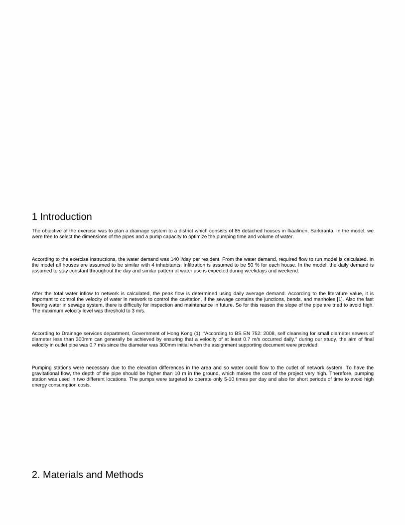
Next, the consumption pattern was developed (Figure 1). Peak demand was calculated using the graph given in exercise. The consumption pattern wasmodified from the Harjuniitty pattern used in the water supply exercise. Peak usage in this model was 7.4 times higher than average usage and it wasassumed the peak inflow would be observed at 7-8 pm.

2.1 Water Pattern and Pipe Dimensioning

Figure 1. Pattern used during the exercise.

All houses were assigned with water consumption of average 560 liters per day using the pattern and it was assumed that the discharge to manholesequals the water use. 50% to total inflow amount of water was assigned as additional infiltration of water to the junction. So the total amount of water inflowto the junction is assigned as 150% of water consumed.

Manholes were place on the street with initial depth of 2 meters. The maximum distance between two manholes was about 40-50 meters. Circularpipelines were used for all gravity pipelines whereas force main pipe was used for the pumping pipeline with surcharge depth of 50 m. Initially, allmanholes were connected using pipe size of 300B (cemented pipe). All other pipe parameters were calculated by the FCGswmm and they were notmodified. And later changed to PEH type with different dimension [2].

2.2 Storage and Pumping

[Figure 2: Water elevation profile from node PR-2 to J6)]

From figure 2 it can be observed that water should travel to the higher elevation from lower elevation and the suitable solutions are either excavating deepinto the soil or having the pumping station to make water flow in the network. Since the head to overcome was around 20 meter so, the suitable option ishaving the pumping station to pump the water. Also similar condition is observed in junction node 3d5 and 3c in the model. So during this exercise twopumping station with two storage unit are modelled.

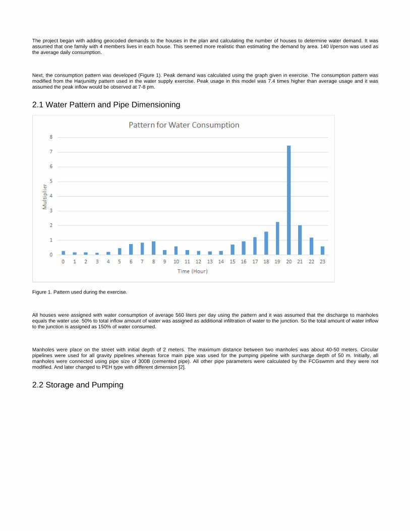
Since the ground elevation was higher in two different junction label as pr9 and 3d3, storage tank capacity of the pumping stations were modified. Eachpumping station has one water collection unit and 2 pumps. To operate the pump, pump curves were assigned (Figures 3 and 4). Initial flow rate wasassigned to be 1 lps with head elevation of 27 m including the flow resistance to overcome for pumping. After the pumps were assigned also the pumpingstartup depth was placed.

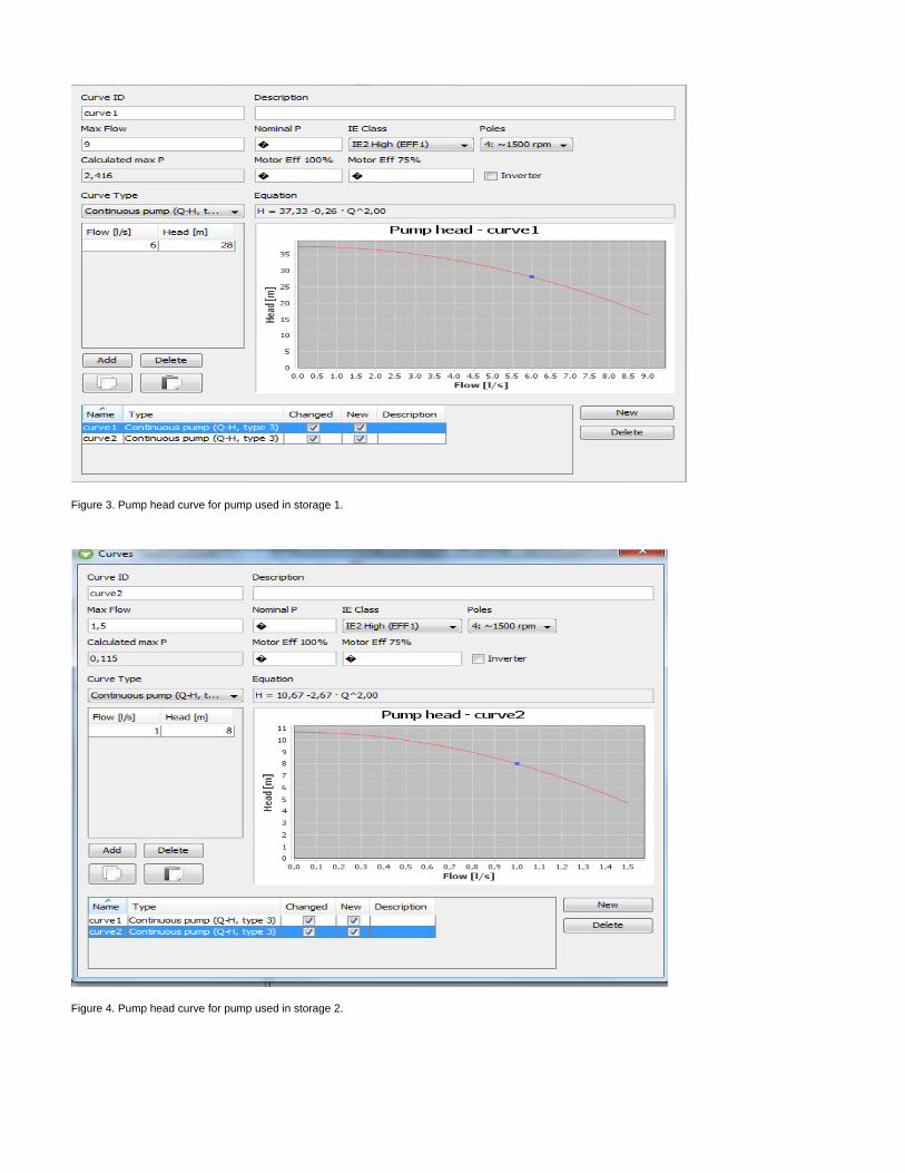
Figure 3. Pump head curve for pump used in storage 1.

Figure 4. Pump head curve for pump used in storage 2.

Table 1. Specification of pumps used in two different locations in the model.

 

  Flow (l/s) Head (m)

Curve1 6 28

Curve 2 1 8

 

Different pump head and flow were used to lower the pump operating time, so electricity consumption could be controlled and enough head would begenerated to pump the water (Table 1).

After defining the pump curve, the dimensions of the storage tank were assigned (Table 2).

Table 2. Dimension of the storage unit used in the model.

 

Storage Unit Depth (m) Base Area (m)

Storage-1 2 4

Storage-2 1 2

 

The final dimension of pipes are mentioned in annex 1 in this report. Higher depth and surface area was assigned to storage unit 1, so large amounts ofwater could be stored if any pump stops working. The basic principle is to avoid flooding and run pumps for a longer periods of time. Pumps are operatingautomatically with different startup depth and shutoff depth as shown in Table 3.

 

After defining the storage unit, the pump settings were separately assigned for all pumps used in the model.

Table 3. Description of the pumping station with the startup depth and shutoff depth.

 

Name Storage Name End

Curve Startup depth (m) Shutoff depth(m)

Pump 4 Storage-1 1 Curve1 0,8 0,2

Pump 3 Storage-1 1 Curve1 0,9 0,2

Pump 2 Storage-2 1 Curve2 0,9 0,2

Pump 1 Storage-2 1 Curve2 0,8 0,2

 

After the setup of all physical units in the model, the model was run, errors detected and fixed to obtain a smaller continuity error. The iteration process isdescribed in Figure 5.

After the first iteration, dimension of pipes were reduced from 300 mm to 200 PEH to main network and 180 PEH for branch gravity sewers and 110 PEHfor pressured pipe and manhole depths were fixed to obtain the gravitational flow in all manholes. The other information about the manhole is available inthe annex 2 After verifying the water flow direction and slope of pipe line, the model was run again.

2.3 Iterative process for model

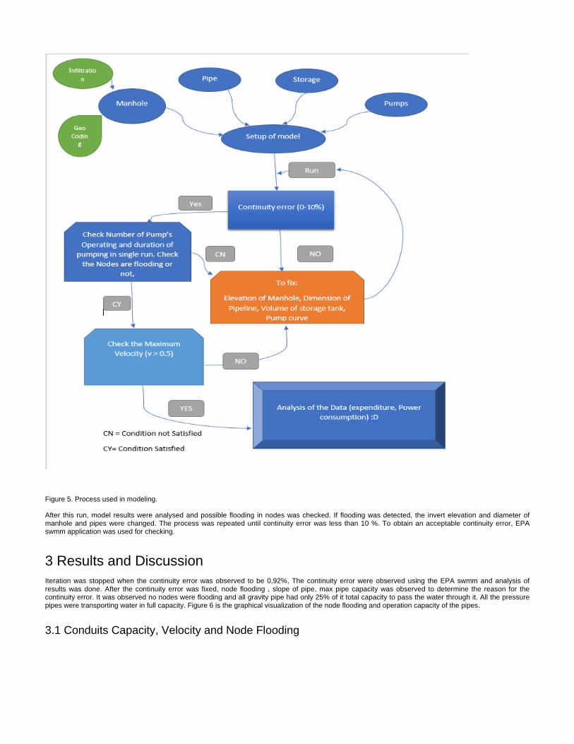
Figure 5. Process used in modeling.

After this run, model results were analysed and possible flooding in nodes was checked. If flooding was detected, the invert elevation and diameter ofmanhole and pipes were changed. The process was repeated until continuity error was less than 10 %. To obtain an acceptable continuity error, EPAswmm application was used for checking.

3 Results and DiscussionIteration was stopped when the continuity error was observed to be 0,92%, The continuity error were observed using the EPA swmm and analysis ofresults was done. After the continuity error was fixed, node flooding , slope of pipe, max pipe capacity was observed to determine the reason for thecontinuity error. It was observed no nodes were flooding and all gravity pipe had only 25% of it total capacity to pass the water through it. All the pressurepipes were transporting water in full capacity. Figure 6 is the graphical visualization of the node flooding and operation capacity of the pipes.

3.1 Conduits Capacity, Velocity and Node Flooding

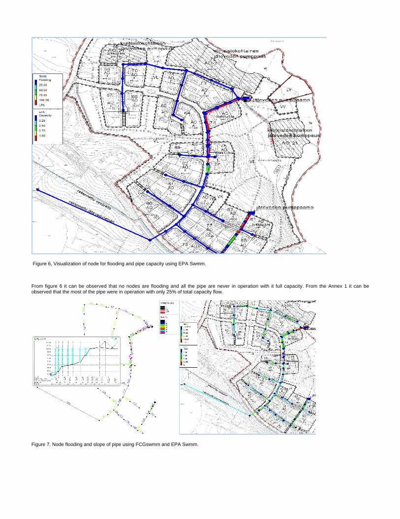
 Figure 6, Visualization of node for flooding and pipe capacity using EPA Swmm.

From figure 6 it can be observed that no nodes are flooding and all the pipe are never in operation with it full capacity. From the Annex 1 it can beobserved that the most of the pipe were in operation with only 25% of total capacity flow.  

Figure 7. Node flooding and slope of pipe using FCGswmm and EPA Swmm.

Also observing the node flooding from the FCG net, it was observed that no node were flooding. With the setting of the pump no storage unit wereflooding. It was observed that only 3 pipe (condu (p7), other pressure pipe had higher slope than 5 cm per meter. Although the maximum velocity wastarget to 0.7 m/s for flushing but the target was only achieved in 20 pipe line (Annex 2). Although the minimum maximum velocity was observed in thecond-45 which is 0.0765 m/s. The maximum velocity was observed in the conduct 41 with velocity of 1,34m/s. The minimum velocity of water flow wasobserved in storage 1 which could be increased by increasing the pumping setting. The initial setting of pumping is the main reason for the minimumvelocity  in the conduit 45. Due to the large inflow and 3% of slope in pipe the velocity is higher.

3.2 Storage Tank, Pumping and Water Balance

During this study water level at tank were studied to determine the capacity of pumping and also to observe to determine if the backup pump s alsooperating to maintain the water volume in the tank. From figure in 7, it can be observed that water label is always below the 0.9m. This suggests that theback pump was not in used during the peak water use. As a conclusion, only have a single backup pump is enough for this sewage network if thespecification of the pump is used according to table 1.

Figure 8. Total outflow from the outflow node and depth of water in pipe with diameter of 300mm (conduit 1) and water level at storage 1 and Inflow ofwater at node of pressure pipe from storage 1.

From Figure 8 it can be observed that maximum outflow is 3,2 lps from the node o1 (outflow)/ cond-1 and depth of the water in the outflow pipeline is 40mm which is around 25% of the total diameter of pipeline. This indicates that the sewage model can handle rainfall and also flooding could be controlled inthe nodes before the outflow. Pump starts when the water level in storage is around 0.9 m, pumps are automatically operated and from figure 8 it can beobserved that peak outflow from the conduit-1 when the water from the storage pump is observed.

Two small bumps in figure 9 presents the pumping of water from the storage 2 in modelling, The water level and flow at pumping station in storage 2 ispresented in figure 10.

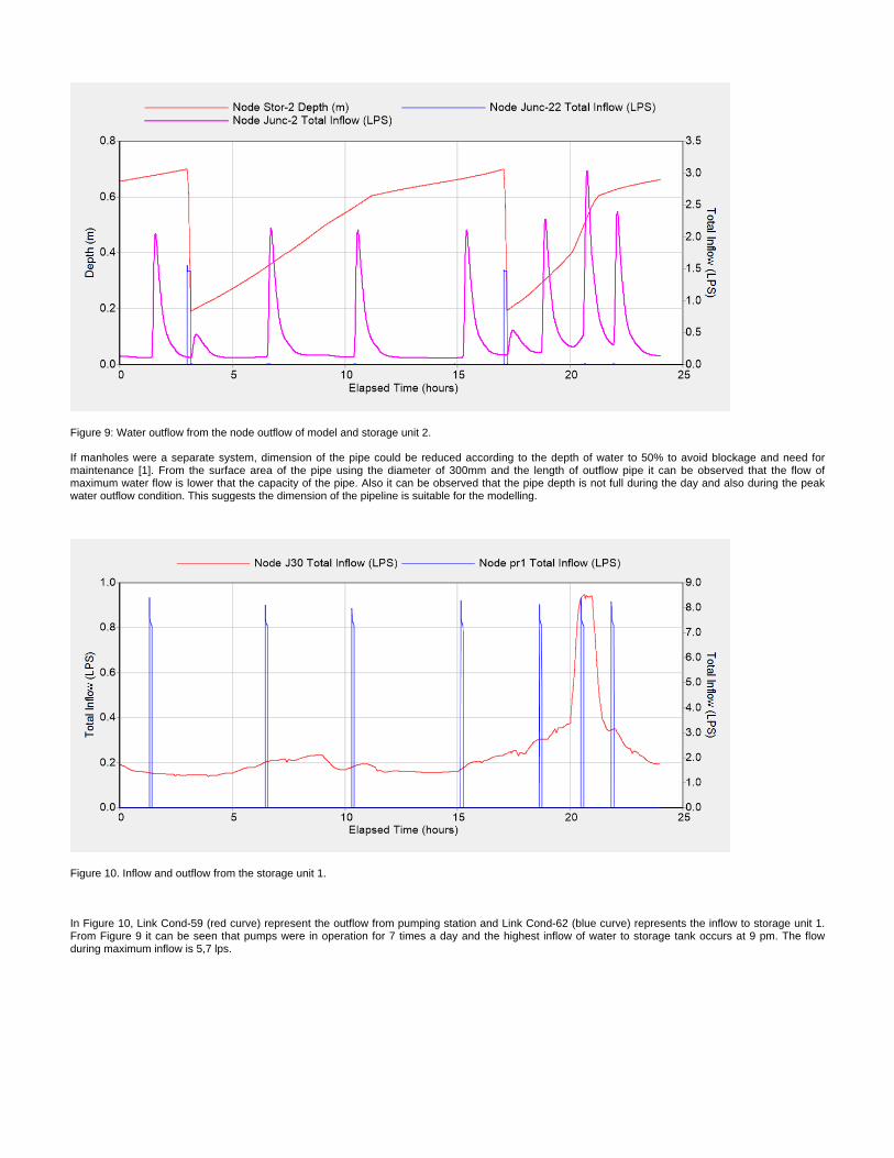
Figure 9: Water outflow from the node outflow of model and storage unit 2.

If manholes were a separate system, dimension of the pipe could be reduced according to the depth of water to 50% to avoid blockage and need formaintenance [1]. From the surface area of the pipe using the diameter of 300mm and the length of outflow pipe it can be observed that the flow ofmaximum water flow is lower that the capacity of the pipe. Also it can be observed that the pipe depth is not full during the day and also during the peakwater outflow condition. This suggests the dimension of the pipeline is suitable for the modelling.

Figure 10. Inflow and outflow from the storage unit 1.

In Figure 10, Link Cond-59 (red curve) represent the outflow from pumping station and Link Cond-62 (blue curve) represents the inflow to storage unit 1.From Figure 9 it can be seen that pumps were in operation for 7 times a day and the highest inflow of water to storage tank occurs at 9 pm. The flowduring maximum inflow is 5,7 lps.

Figure 11. Inflow and outflow from the storage unit 2.

The pumps in storage tank were in operation only from two time. Water inflow to node 3d5 is only observed twice.

From Figure 11 it can be concluded that pumps are used 7 times a day for a very short period of time during 1 pumping cycle. The detailed numbers fromthe hours the pumps operated are shown in Table 4 and water balance in table 5.

Table 4. Pumping inputs and output.  (Data is obtained from EPA SWMM)

 

Table 5. Water balance calculation from the storage unit 1 and 2.

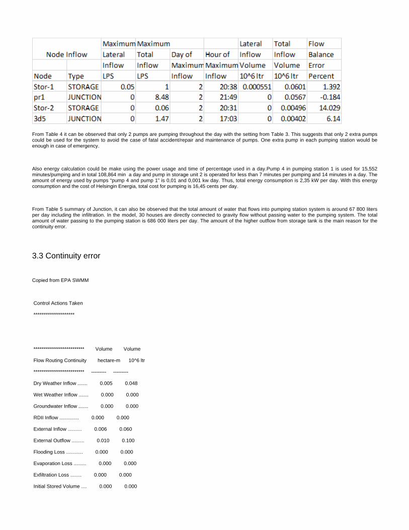
From Table 4 it can be observed that only 2 pumps are pumping throughout the day with the setting from Table 3. This suggests that only 2 extra pumpscould be used for the system to avoid the case of fatal accident/repair and maintenance of pumps. One extra pump in each pumping station would beenough in case of emergency.

Also energy calculation could be make using the power usage and time of percentage used in a day.Pump 4 in pumping station 1 is used for 15,552minutes/pumping and in total 108,864 min  a day and pump in storage unit 2 is operated for less than 7 minutes per pumping and 14 minutes in a day. Theamount of energy used by pumps “pump 4 and pump 1” is 0,01 and 0,001 kw day. Thus, total energy consumption is 2,35 kW per day. With this energyconsumption and the cost of Helsingin Energia, total cost for pumping is 16,45 cents per day.

From Table 5 summary of Junction, it can also be observed that the total amount of water that flows into pumping station system is around 67 800 litersper day including the infiltration. In the model, 30 houses are directly connected to gravity flow without passing water to the pumping system. The totalamount of water passing to the pumping station is 686 000 liters per day. The amount of the higher outflow from storage tank is the main reason for thecontinuity error.

3.3 Continuity error

Copied from EPA SWMM

 Control Actions Taken

 *********************

 

 **************************        Volume        Volume

 Flow Routing Continuity        hectare-m      10^6 ltr

 **************************     ---------     ---------

 Dry Weather Inflow .......         0.005         0.048

 Wet Weather Inflow .......         0.000         0.000

 Groundwater Inflow .......         0.000         0.000

 RDII Inflow ..............         0.000         0.000

 External Inflow ..........         0.006         0.060

 External Outflow .........         0.010         0.100

 Flooding Loss ............         0.000         0.000

 Evaporation Loss .........         0.000         0.000

 Exfiltration Loss ........         0.000         0.000

 Initial Stored Volume ....         0.000         0.000

 Final Stored Volume ......         0.001         0.007

 Continuity Error (%) .....         0.917

 

 

 *************************

 Highest Continuity Errors

 *************************

 Node 3d4 (13.96%)

 Node Stor-2 (12.12%)

 Node Junc-22 (10.55%)

 Node 3d5 (5.69%)

 Node J30 (1.86%)

 

 

 ***************************

 Time-Step Critical Elements

 ***************************

 None

 

 

 ********************************

 Highest Flow Instability Indexes

 ********************************

 Link Cond-59 (1)

From the analysis of the result using epa swmm, it can be observed that there is extra water as input to the system than the assigned input to the geocodeand infiltration. From the continuity error value it can be observed that node 3d4 which is the discharge manhole in pressure pipeline from the storage unit2 has highest continuity error. And the node with label in Junc- 22 have the higher positive continuity error. Also it can be observed that the total amount ofwater stored in the system is only 7000 liter in a day. The amount of water stored is in storage tank since the pumps shut-off when the water level is 0.2 min the storage unit. From the EPA swmm it can be observed that the Pipe label 59 is the critical in modeling.  

When the model was run with FCG net the continuity error observed was -48.8%. So the pipe profile from the storage unit 2 to to node 3 was observedwhere is the main water loss in the system even there is no flooding was observed.

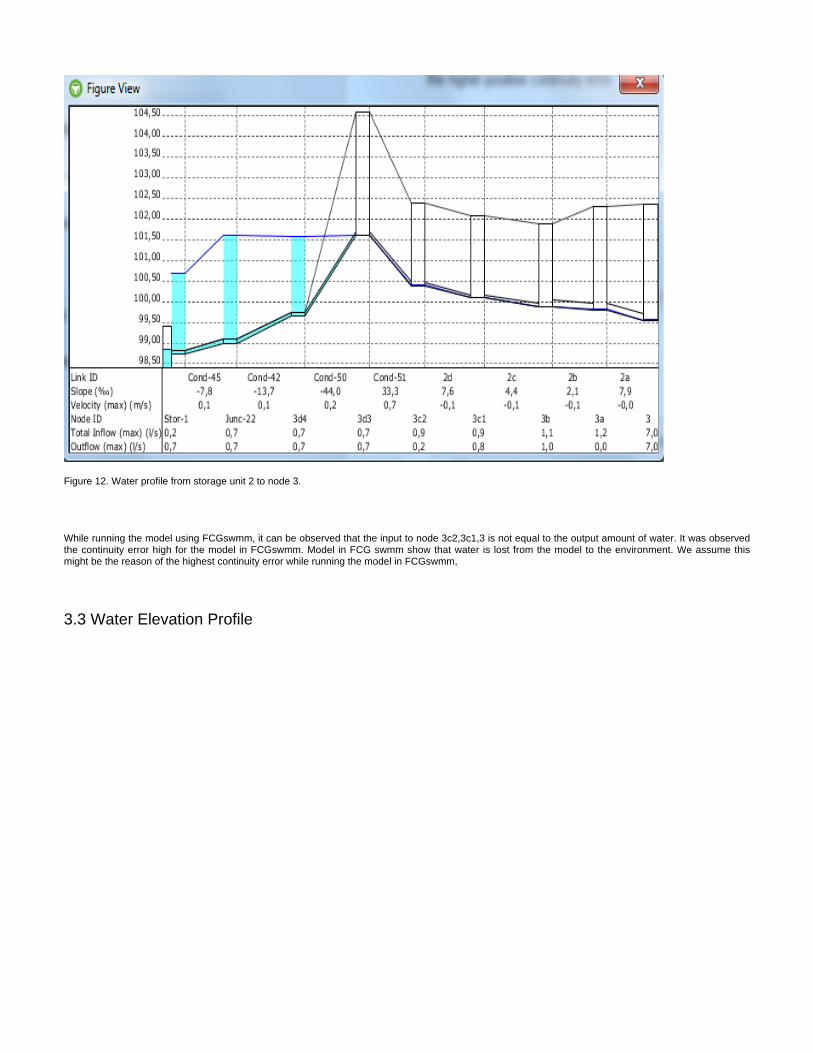
Figure 12. Water profile from storage unit 2 to node 3.

While running the model using FCGswmm, it can be observed that the input to node 3c2,3c1,3 is not equal to the output amount of water. It was observedthe continuity error high for the model in FCGswmm. Model in FCG swmm show that water is lost from the model to the environment. We assume thismight be the reason of the highest continuity error while running the model in FCGswmm,

3.3 Water Elevation Profile

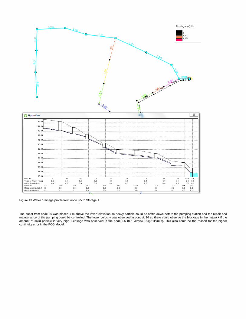
Figure 13 Water drainage profile from node j25 to Storage 1.

The outlet from node 30 was placed 1 m above the invert elevation so heavy particle could be settle down before the pumping station and the repair andmaintenance of the pumping could be controlled. The lower velocity was observed in conduit 16 so there could observe the blockage in the network if theamount of solid particle is very high. Leakage was observed in the node j25 (0,5 l/km/s), j24(0,1l/km/s). This also could be the reason for the highercontinuity error in the FCG Model.

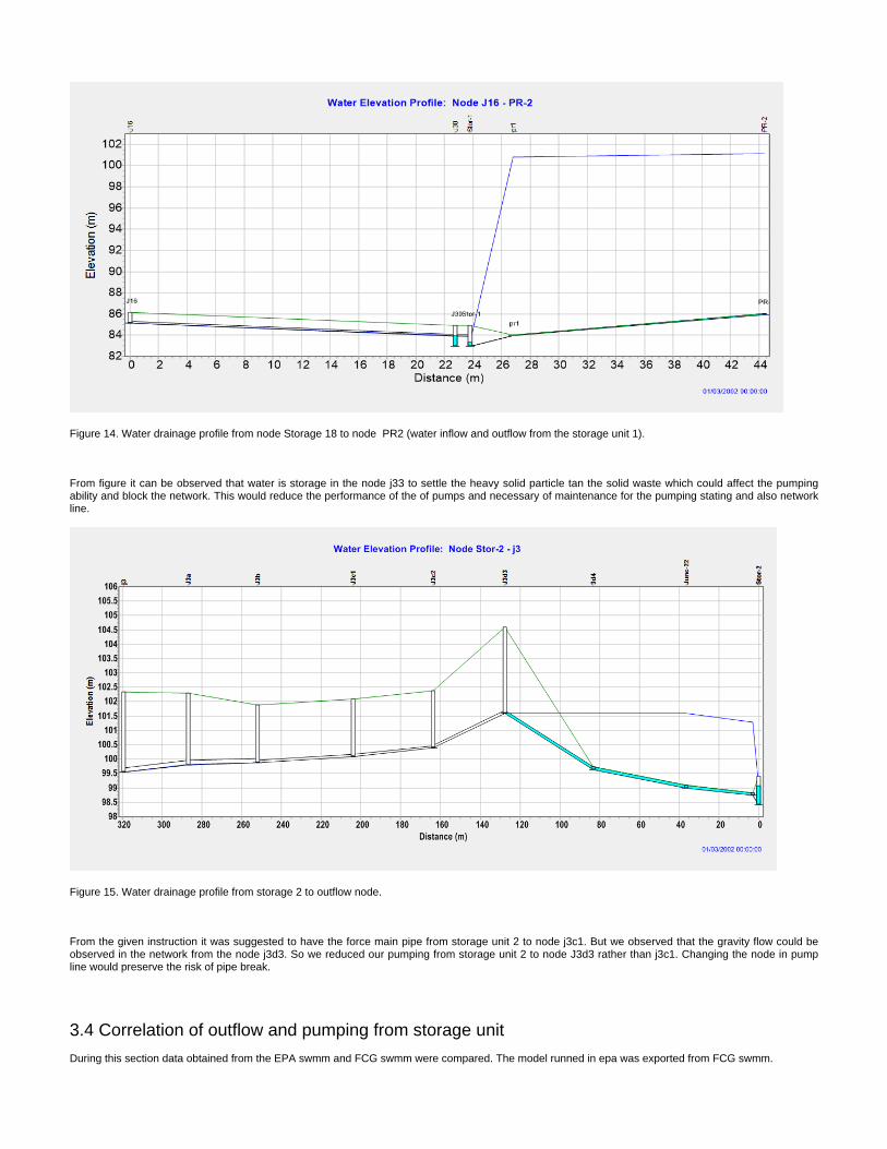
Figure 14. Water drainage profile from node Storage 18 to node  PR2 (water inflow and outflow from the storage unit 1).

From figure it can be observed that water is storage in the node j33 to settle the heavy solid particle tan the solid waste which could affect the pumpingability and block the network. This would reduce the performance of the of pumps and necessary of maintenance for the pumping stating and also networkline.

Figure 15. Water drainage profile from storage 2 to outflow node.

From the given instruction it was suggested to have the force main pipe from storage unit 2 to node j3c1. But we observed that the gravity flow could beobserved in the network from the node j3d3. So we reduced our pumping from storage unit 2 to node J3d3 rather than j3c1. Changing the node in pumpline would preserve the risk of pipe break.

3.4 Correlation of outflow and pumping from storage unit

During this section data obtained from the EPA swmm and FCG swmm were compared. The model runned in epa was exported from FCG swmm.

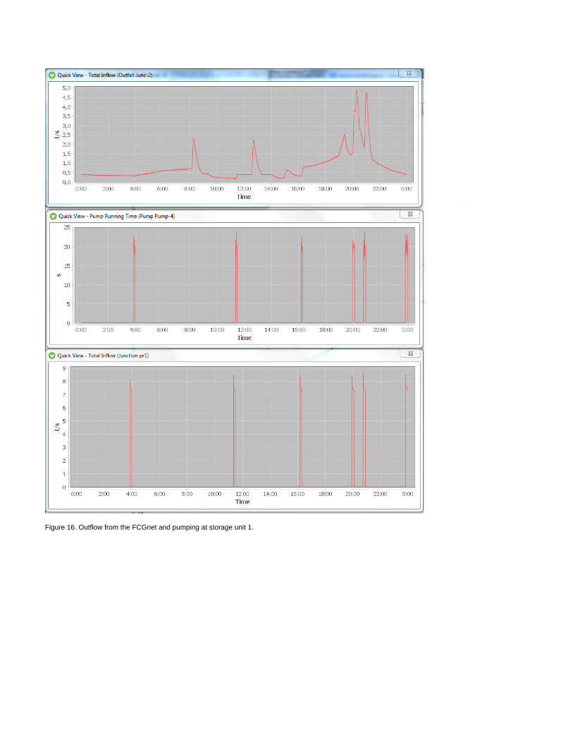
Figure 16. Outflow from the FCGnet and pumping at storage unit 1.

Figure 17. Outflow from the EPA swmm and pumping at storage unit 1.

From the figure 16 it can be observed that the pump in storage unit 1 was operated only 6 time. Observing the total inflow from the outflow node, thepattern for water outflow differs and the outflow is higher during the evening hours of 19-22 pm. And in the epa swmm model the total inflow to outflownode was 3.0 lps and pumps were operated 7 time with epa swmm. Observing the graph it can be observed that outflow and pumping have very closecorrelation in epa swmm where as there is very slight correlation in FCG net. The outflow in epa swmm model is observed higher when the pumps areoperated and also the higher outflow is observed after very delay of pumping. This make sense since water takes time to flow in the network. So we thinkthe data obtained from EPA swmm is more reliable than FCG net.

4 ConclusionsThe total length of the pipe line used  was 2739.559 meter in designing the network. Determining the appropriate dimension of the pipe and slope isimportant for obtaining the target velocity.   the  This modeling exercise showed that careful planning is crucial also, or perhaps especially, in designingwastewater networks because flaws in design can lead to serious bottleneck nodes and well as conduits in network  as a result which leads to waste timeand money. Time spent on planning pays off and reduces the need for making changes later on. During the planning the sewage network it is alwaysimportant to focus on invert elevation, depth of the manhole and slope to obtain desired velocity to avoid the flooding. To be in the safe side it is importantto have at least 50% of flow capacity of the pipe line.

Modelling the network was done on based on the 4 people per house but it would be recommended to perform the modeling with resident of 6 people perhouse. This would increase the capacity of inflow of the wastewater and help to determine the capacity of the pipe in worst case scenario.  Also from thedata observed for capacity of the pipeline, it can be concluded that the system could be function without any modification if the additional resident connectto the network with small modification of the pumps specification or settings. Also the pipe slope could be increased to increase the water flow velocity andthe dimension could be also decreased if the there is no any further city/rural development plans in the network.

Documenting the phases and making notes proved out to be an essential part of the process as it helped to trace possible sources of errors, shareinformation and justify decisions. Summing up the main outcomes and lessons learned after the modeling process is equally important: these are a greathelp when solving similar problems in other modeling projects.

The final result depends on the number and location of junctions, pipe sizing, pump settings. Also it would be interesting to include some 1- year  designstorm to the catchment and see the performance of the model and if necessary perform the necessary modification. But as a conclusion, observing thecontinuity error the model should be performing well in long term only further development could be done to improve the maximum velocity in someconduit.

Feedback from exercise:In the model manholes had to be deeper than the recommended depth to make gravity sewers work, it would be nice to know how this would besolved in a real modeling caseIn the exercise there’s a separate pumping station for 4 houses, is this realistic?We observed the outflow volume difference in the two different application while running the model. We were us confused and we checkedcorrelation between the pump operation time and outflow. The outflow from EPA swmm make more sense than the outflow from the FCG SWMMso, we think that there is some problem in FCG swmm application.

It would be nice if we were provided the flowchart what step to follow while making the model and necessary modification.We also had some problem while loading the background map, it would also nice to have small tutorial file for running the FCG swmm and wouldbe helpful if we were provided some presentation slide for FCGswmm. It is difficult to find any help from google or youtube while running themodel.We think the assistance during the exercise session was really helpful and we really appreciate Kaleva’s time.During the exercise, we basically run the model targeting the continuity error and we think we were lacking the background technical knowledgeto explain how the model actually works.We also think it would be nice if we were recommended any books for determining the technical detail of pipes and slope. Although the manningequation and head loss equation was utilized during the exercise to target the slope, diameter and velocity.

Reference

[1] Sweage Manual, Key Planning Issues and Gravity Collection System, Draiange Departnment , Government of Hong KongOnline Avaiable:  http://www.dsd.gov.hk/EN/Files/Technical_Manual/technical_manuals/Sewerage_Manual_1_Eurocodes.pdf

[2]Energiavirasto (2016). Sähkön hintatilastot. Available at: http://www.energiavirasto.fi/sahkon-hinta

[3] Plastic pipe Institute, Meeting the challenge of the 21st Century. Online Available at:

https://plasticpipe.org/pdf/high_density_polyethylene_pipe_systems.pdf

Annex 1

Annex 2