remote sensing of environment - vliz · comparison of three seawifs atmospheric correction...

Remote Sensing of Environment 115 (2011) 1955–1965

Contents lists available at ScienceDirect

Remote Sensing of Environment

j ourna l homepage: www.e lsev ie r.com/ locate / rse

Comparison of three SeaWiFS atmospheric correction algorithms for turbid watersusing AERONET-OC measurements

Cédric Jamet a,b,⁎, Hubert Loisel a,b, Christopher P. Kuchinke c, Kevin Ruddick d, Giuseppe Zibordi e, Hui Feng f

a Univ Lille Nord de France, ULCO, LOG, F-62930 Wimereux, Franceb CNRS, UMR 8187, F-62930 Wimereux, Francec Department of Physics, University of Miami, PO Box 248046, Coral Gables, FL 33124, USAd Management Unit of the North Sea Mathematical Models (MUMM), Royal Belgian Institute for Natural Sciences (RBINS), 100 Gulledelle, B-1200 Brussels, Belgiume Joint Research Centre, Institute for Environment and Sustainability, Global Environment Monitoring Unit, Ispra, 21020, Italyf Ocean Process Analysis Laboratory, Institute for the Study of Earth, Oceans and Space, University of New Hampshire, Durham, NH 03824, USA

⁎ Corresponding author at: Univ Lille Nord de France, UFrance.

E-mail address: [email protected] (C. Jam

0034-4257/$ – see front matter © 2011 Elsevier Inc. Aldoi:10.1016/j.rse.2011.03.018

a b s t r a c t
a r t i c l e i n f o
Article history:Received 4 August 2010Received in revised form 16 March 2011Accepted 21 March 2011Available online 14 April 2011

Keywords:Ocean colorAtmospheric correctionRemote sensingValidationAERONET-Ocean Color

Theuseof satellites tomonitor the color of theoceanrequires effective removal of the atmospheric signal. This canbe performed by extrapolating the aerosol optical properties in the visible from the near-infrared (NIR) spectralregion assuming that the seawater is totally absorbant in this latter part of the spectrum. However, the non-negligible water-leaving radiance in the NIRwhich is characteristic of turbid waters may lead to an overestimateof the atmospheric radiance in the whole visible spectrum with increasing severity at shorter wavelengths. Thismay result in significant errors, if not complete failure, of various algorithms for the retrieval of chlorophyll-aconcentration, inherent optical properties and biogeochemical parameters of surface waters.This paper presents results of an inter-comparison study of three methods that compensate for NIR water-leaving radiances and that are based on very different hypothesis: 1) the standard SeaWiFS algorithm (Stumpf etal., 2003; Bailey et al., 2010) based on a bio-optical model and an iterative process; 2) the algorithm developedby Ruddick et al. (2000) based on the spatial homogeneity of the NIR ratios of the aerosol and water-leavingradiances; and 3) the algorithm of Kuchinke et al. (2009) based on a fully coupled atmosphere–ocean spectraloptimization inversion. They are compared using normalized water-leaving radiance nLw in the visible. Thereference source for comparison is ground-based measurements from three AERONET-Ocean Color sites, one inthe Adriatic Sea and two in the East Coast of USA.Based on the matchup exercise, the best overall estimates of the nLw are obtained with the latest SeaWiFSstandard algorithm version with relative error varying from 14.97% to 35.27% for λ=490 nm and λ=670 nmrespectively. The least accurate estimates are given by the algorithm of Ruddick, the relative errors beingbetween 16.36% and 42.92% for λ=490 nm and λ=412 nm, respectively. The algorithm of Kuchinke appears tobe the most accurate algorithm at 412 nm (30.02%), 510 (15.54%) and 670 nm (32.32%) using its defaultoptimization and bio-optical model coefficient settings.Similar conclusions are obtained for the aerosol optical properties (aerosol optical thickness τ(865) and theÅngström exponent, α(510, 865)). Those parameters are retrieved more accurately with the SeaWiFS standardalgorithm (relative error of 33% and 54.15% for τ(865) and α(510, 865)).A detailed analysis of the hypotheses of the methods is given for explaining the differences between thealgorithms. The determination of the aerosol parameters is critical for the algorithm of Ruddick et al. (2000)while the bio-optical model is critical for the algorithm of Stumpf et al. (2003) utilized in the standard SeaWiFSatmospheric correction and both aerosol and bio-optical model for the coupled atmospheric–ocean algorithm ofKuchinke. The Kuchinke algorithm presents model aerosol-size distributions that differ from real aerosol-sizedistribution pertaining to the measurements. In conclusion, the results show that for the given atmospheric andoceanic conditions of this study, the SeaWiFS atmospheric correction algorithm is most appropriate forestimating the marine and aerosol parameters in the given turbid waters regions.

LCO, LOG, F-62930 Wimereux,

et).

l rights reserved.

© 2011 Elsevier Inc. All rights reserved.

1. Introduction

Coastal waters are ecologically very important and also a majorresource for human populations because they contribute to a largeshare of the world fisheries catch and support the rapidly growing

http://dx.doi.org/10.1016/j.rse.2011.03.018

mailto:[email protected]

http://dx.doi.org/10.1016/j.rse.2011.03.018

http://www.sciencedirect.com/science/journal/00344257

1956 C. Jamet et al. / Remote Sensing of Environment 115 (2011) 1955–1965

aquaculture industry. These waters are generally identified as Case IIwaters (Morel & Prieur, 1977), as opposed to Case I waters, becausetheir optical properties cannot be solely defined as a function of asingle phytoplankton-related parameter (due to contributions fromnon-co-varying terrestrial constituents such as detritus and coloreddissolved organic matter (CDOM) from bottom resuspension andterrestrial origin). Because of the complexity of Case II waters, sincethe late 1970s most of the quantitative applications of ocean colorremote sensing focused on Case I waters andweremostly restricted tothe determination of the abundance and distribution of phytoplank-ton chlorophyll-a.

Since the Coastal Zone Color Scanner (CZCS) proof-of-concept oceancolor mission (operating from 1978 to 1986), spaceborne monitoring ofchlorophyll-a concentration has become well established and main-tained through several satellite sensors including the Sea-ViewingWideField-of-View Sensor (SeaWiFS) launched in August 1997, the ModerateResolution Imaging Spectroradiometers (MODIS) onboard the Terra andAqua platforms in 1999 and 2002, respectively, and the MediumResolution Imaging Spectrometer (MERIS) in 2002. The focus of thepresent study is on SeaWiFS, which now offers more than 13 years ofdata, giving the unique opportunity to study the long-term variability ofthe seawater properties at global and regional scales. This sensor has 6spectral bands in the visible centered at λ=412, 443, 490, 510, 555, and670 nm and two bands in the near-infrared centered at λ=765 and865 nm.

The use of satellites to monitor the color of the ocean requireseffective removal of the contribution of the atmosphere (due toabsorption by gasses and aerosols, and scattering by air molecules andaerosols) to the total signal measured by the remote sensor at the top ofthe atmosphere, Ltoa: the socalled “atmospheric correction”process. Themethods for removing the contribution of the atmosphere to the totalmeasured signal exploit the high absorption by seawater in the red andnear-infrared spectral regions. In open seawater, i.e. where generallychlorophyll-a concentration and related pigments and co-varyingmaterials (like detritus) determine the optical properties of the ocean,seawater can be considered to absorb all light in the NIR so that thesignal observedby the satellite sensor in this spectraldomain is assumedto be entirely due to the atmospheric path radiance (LA) and sea surfacereflectance. This is not always the case when considering turbid waters(generally coastal optically complex waters). In these waters phyto-plankton pigment and detritus, as well as suspended sediment,contribute toNIR backscatter. The resultingNIRwater-leaving radiancesintroduce two sources of error into the removal of the aerosol. First, thetotal aerosol reflectance is overestimated as some of the total radiance(Ltoa) at both 765 and 865 nm comes from the seawater. Second, as theabsorption and scattering properties of seawater change from 765 to865 nm, the selection of the appropriate atmospheric model is affected,causing an error in the extrapolation of LA to shorter wavelengths. As aresult, LA is overestimated at all bands with increasing values at shorterwavelengths, even possibly leading to negativewater-leaving radiancesin the blue bands in coastal waters (Siegel et al., 2000). This results insevere errors, if not complete failure, for various algorithms to retrievechlorophyll-a concentration and inherent optical properties relying onthe spectral values of the water-leaving radiance.

To solve this problem, several atmospheric correction algorithmshave been developed to process SeaWiFS data when normalizedwater-leaving radiance nLw is non-negligible at NIR wavelengths(Bailey et al., 2010; Gould et al., 1998; Hu et al., 2000; Kuchinke et al.,2009a; Land & Haigh, 1996; Lavender et al., 2005; Oo et al., 2008;Ruddick et al., 2000; Shanmugam & Ahn, 2007; Stumpf et al., 2003).The existing large number of coastal water algorithms requires theirinter-comparison to assess their accuracy since they are often basedon quite different physical assumptions. However, only a few studieshave been made to evaluate several algorithms from in-situmeasurements (Banzon et al., 2009 for instance). More recently, acomparison of the standard atmospheric correction algorithms of the

SeaWiFS, MODIS, MERIS, OCTS/GLI and POLDER sensors for the clearand turbid ocean has been made by a working group of theInternational Ocean Color Coordinating Group (IOCCG, 2010). Thiskind of exercise is fundamental to understand and compare retrievalsfrom different sensors using different algorithms.

In this paper, three SeaWiFS data processing algorithms currentlyavailable in the SeaWiFS Data Analysis System (SeaDAS, Fu et al.,1998; Baith et al., 2001) are compared: the SeaWiFS standardalgorithm (Bailey et al., 2010; Stumpf et al., 2003) and those proposedby Ruddick et al. (2000) and by Kuchinke et al. (2009a). The first twoalgorithms are based on the standard atmospheric correction ofGordon andWang (1994), from herein referred to as GW94, and havebeen compared by Ransibrahmanakul et al. (2005), showing that theSeaWiFS standard algorithm provided the best estimates of thenormalized water-leaving radiances using in-situ data along the U.S.coasts. The Kuchinke et al. (2009a) algorithm is an extension of theatmospheric correction of Chomko and Gordon (1998) and has beencompared with the standard algorithm in Kuchinke et al. (2009b).This paper presents the first outcome of the ICAC inter-comparisonproject by comparing algorithms with in situ measurements ofnormalized water-leaving radiance (nLw) made in coastal watersthrough the AERONET-Ocean Color network (thereafter AERONET-OC) of autonomous radiometers (Zibordi et al., 2006b, 2009). Thisnetwork constitutes a unique dataset for assessment of the accuracyof satellite products in different coastal waters.

The results presented in this paper are based on data obtained withnew SeaWiFS reprocessing released by NASA in fall 2009 and calledR2009. The SeaWiFS standard NIR ocean contribution correctionalgorithm developed by Stumpf et al. (2003) and its update version(Bailey et al., 2010) is hereafter named S03, the NIR ocean contributioncorrectionmethoddevelopedbyRuddick et al. (2000) is namedR00 andthe atmospheric correction of Kuchinke et al. (2009a) is named K09. Inthe following sections, a short description of the three algorithms ispresented showing their assumptions together with the details of the insitu measurements used for comparisons and the match-up protocol.The last two sections present the comparison analysis and a discussionon the limitations of the three algorithms.

2. Algorithms

The standardNIRocean contribution correctionmethod S03 andR00evaluated in this study are based on the atmospheric correctionalgorithm initially developed for Case I waters by GW94. Thesealgorithms extend the GW94 approach to waters where the blackpixel assumption no longer holds (Siegel et al., 2000). The thirdalgorithm, K09, contains its own independent atmospheric correctionalgorithm.

The top-of-atmosphere radiative signal can be expressed as:

ρcor λð Þ = ρa λð Þ + ρra λð Þ + t λð Þ⋅ρw λð Þ = ρA λð Þ + t� λð Þ⋅ρw λð Þ ð1Þ

where ρcor(λ) is the top-of-atmosphere signal corrected for gasabsorption, Rayleigh scattering, whitecaps and glitter (Gordon, 1997),ρA(λ) is the reflectance due to the aerosol scattering and theinteraction between molecular and aerosol scattering reflectance,t⁎(λ) is the diffuse transmittance through the atmosphere and ρw(λ),the water-leaving reflectance. The goal of the atmospheric correctionprocess is to quantify ρA(λ) to determine ρw(λ). The latter can then beused to assess the optical and biogeochemical properties of theseawater. In the rest of the paper, we will focus on the radiance

instead of the reflectance, defined as: L λð Þ = ρ λð Þ⋅F0⋅ cosθ0π

:

2.1. GW94-based with iterative procedure

The S03method is based on an iterative procedurewhich is used toavoid the over-correction of the atmospheric signal. The procedure is

1957C. Jamet et al. / Remote Sensing of Environment 115 (2011) 1955–1965

based on the original SeaWiFS processing code using GW94atmospheric model. The goal is to remove Lw(NIR) from Lcor(NIR) sothat only the atmospheric component of Lcor(NIR) is input into GW94.The iteration used Lcor(NIR) as input into GW94 in order to solve forLw(670). Then, Lw(670) is used through a bio-optical model todetermine Lw(NIR). This model is used to determine the backscatter at670 nm, and specifically considers inorganic particles. This solutionrequires compensation for absorption by chlorophyll-a, detritalpigments and colored dissolved organic matter (CDOM). These arepropagated to the top of the atmosphere (TOA). This TOA Lw(NIR) isremoved from Lcor(NIR) which is then input into GW94 computation.

2.2. GW94-based with spatial homogeneity of NIR ratios of ρw and ρA

The second algorithm chosen uses an alternative method forestimating the marine contribution in the NIR as proposed by Ruddicket al. (2000). This algorithm replaces the assumption that the water-leaving radiance is zero in the NIR by the assumptions of spatialhomogeneity of the 765/865 nm ratios for aerosol and water-leavingreflectances over the subscene of interest. The ratio of ρA reflectancesat 765 and 865 nm is named ε and is considered as a calibrationparameter to be calculated for each sub-scene of interest. In addition,the ratio of ρw at 765 and 865 nm, named α, is also considered as acalibration parameter and is fixed to a value 1.72 for the SeaWiFSsensor (Ruddick et al., 2000, 2006). These assumptions are used toextend to turbid waters the GW94. Using the definition of α and ε, theequations defining ρA(765) and ρA(865) become:

ρA 765ð Þ = ε 765;865ð Þ: α⋅ρcor 865ð Þ−ρcor 765ð Þα−ε 765;865ð Þ

� �ð2Þ

ρA 865ð Þ = α⋅ρcor 865ð Þ−ρcor 765ð Þα−ε 765;865ð Þ ð3Þ

The atmospheric correction algorithm can be summarized thus:

(1) Enter the atmospheric correction routine (i.e. GW94) to producea scatter plot of Rayleigh-corrected reflectances ρcor(765) andρcor(785) for the region of study. Select the calibration parameterε on the basis of this scatter plot as described later.

(2) Reenter the atmospheric correction routine with data forRayleigh-corrected reflectances ρcor(765) and ρcor(785) anduse Eqs. (2) and (3) to determine ρA(765) and ρA(765), takingaccount of non-zero water-leaving reflectances.

(3) Continue as for the standard GW94 algorithm.

2.3. Spectral optimization algorithm

The algorithm K09 is a turbid-water adaptation of Chomko et al.(2003), named thereafter SOA, with improved atmospheric correctionand scope to regionally tune the bio-optical model. It uses absorbing‘Haze-C’ aerosol models (Chomko & Gordon, 1998) and a bio-opticalreflectance model (Garver & Siegel, 1997, Maritonera et al., 2002;herein referred to as GSM) to provide the top-of-atmosphere (TOA)reflectance. The parameters of both models are then determined byfitting themodeled TOA reflectance to that observed from space, usingnon-linear optimization. Thus, it differs from GW94 in that allparameters are obtained simultaneously using all SeaWiFS bands.This is necessary in absorbing atmospheres where one can only ‘see’aerosol absorption at wavelengths where high multiple scatteringthat exists, namely, the blue region of the visible spectrum. Since theGW94 atmospheric correction only uses NIR bands for its modelselection, it cannot discern coastal aerosol absorption if it exists.

The SOA accounts for non-zero NIRwater leaving reflectance by firstassuming ρw(NIR)=0 to provide initial estimates of ρA, and t* at NIRand visible wavelengths, and ρw at visible wavelengths. The retrieved

apparent optical properties from GSM are then used to determine ρ′w(NIR). The estimate of t*ρ′w(NIR) is then subtracted from the totalreflectance to form the corrected reflectance, i.e.,

ρA NIRð Þ + ρw NIRð Þ½ � Correctedð Þ = ρt NIRð Þ−ρr NIRð Þ−t � NIRð Þρ′w NIRð Þ ð4Þ

and the updated ρA NIRð Þ + ρw NIRð Þ is used to initiate a newoptimization, i.e., improved estimates of atmospheric parametersand subsequent calculation of new water parameters. The procedureiterates until the magnitude of ρw(865) (or its difference acrossconsecutive Case 2 loops, namely delta ρw(865)) falls below 0.0001.Since all models are coupled, the selection of bio-optical coefficients inK09 will have some effect on its atmospheric correction. In this studywe elect to use the SeaDAS-default GSM Case 1 water bio-opticalcoefficients as determined by Maritonera et al. (2002).

3. Data

3.1. Satellite data

The satellite Level-1A data from SeaWiFS, onboard the OrbView-2spacecraft, were acquired from the OBPG ocean color website(Feldman & McClain, 2009). Only the LAC (local-area coverage data)and MLAC (merged LAC, which consolidates all available full-resolution from a single orbit) full-resolution (1 km at nadir) imagerywere considered. The satellite scenes corresponding to field mea-surements have been processed with the SeaDAS software package(version 6.1), using the latest SeaWiFS calibration.

The outputs of the SeaDAS processing are the normalized water-leaving radiancenLw(λ) at centerwavelengthsof412, 443, 490, 510, 555and 667 nm, denoted as nLw(412), nLw(443), nLw(490), nLw(510), nLw(555), nLw(670), respectively, the aerosol optical thickness, atλ=865 nm, τ(865) and the Ångström coefficient determined fromτ(λ) at λ=510 nm and λ=865 nm, α(510, 865), named hereafter,α(510).

3.2. Ground-based measurements

To estimate the accuracy of the values of nLw(λ) obtained from thethree atmospheric correction algorithms, the retrievals were comparedto in situmeasurements of thenormalizedwater-leaving radiance (nLw)from AERONET-OC (Zibordi et al., 2006b, 2009). Three coastal stationswere considered: theMVCO and COVE sites off the East Coast of theUSAand the Acqua Alta Oceanographic Tower (AAOT) in the northernAdriatic Sea identified as Venise in the AERONET-OC database.Evaluations of the MODIS atmospheric and water products for theMVCO station have been published by Feng et al. (2008). Similarcomparisons for the SeaWiFS, MERIS and MODIS products have beenmade for the AAOT and COVE sites (Melin et al., 2007; Zibordi et al.,2006a, 2009). The mean values and the standard deviations of thesedataset are given in Table 1. The atmospheric andmarine features of thethree AERONET-OC sites have been extensively studied in the paper ofZibordi et al. (2009).

The AAOT site (Zibordi et al., 2006b) is located at 45.31°N; 12.50°E,14.8 km off the Venice Lagoon in a frontal region that can becharacterized by either Case I or Case II waters (Berthon & Zibordi,2004). The Case IIwaters as classified by Loisel andMorel (1998), whichrepresent a third of themeasurement conditions, aremostly determinedby the effects of river discharge and local winds. The aerosol type ismostly continental as influencedby atmospheric inputs from thenearbyPo Valley. The dataset covers measurements over 68 months in theperiod from April 2002 to November 2007.

The MVCO site (Feng et al., 2008) is located at 41.33°N; 70.57°W,3 kmfrom the coast. As in the case ofAAOT, there are spatial gradients innLw explained by a large variability in the seawater bio-opticalproperties. The seawater shows presence of highly absorbing dissolved

Table 1Mean values and the standard deviation of in-situ nLw(λ), τ(865) and α(510) for the MVCO, AAOT and COVE stations.

nLw(412) nLw(443) nLw(490) nLw(510) nLw(555) nLw(670) τ(865) α(510)

MVCO x� σ xð Þ 0.45±0.11 0.63±0.19 0.99±0.31 1.11±0.35 1.18±0.38 0.27±0.11 0.054±0.062 1.49±0.46AAOT x� σ xð Þ 0.92±0.30 1.19±0.43 1.64±0.60 1.73±0.60 1.60±0.48 0.29±0.11 0.080±0.060 1.52±0.51COVE x� σ xð Þ 0.61±0.27 0.88±0.31 1.23±0.40 1.35±0.42 1.45±0.42 0.39±0.14 0.045±0.040 1.09±0.62Global x� σ xð Þ 0.85±0.32 1.10±0.44 1.53±0.59 1.62±0.59 1.55±0.48 0.29±0.11 0.070±0.054 1.48±0.55

Table 2Number of matchups for each site and each algorithm.

MVCO AAOT COVE TOTAL nLw(412) b0

S03 20 163 18 201 7R00 19 129 17 165 6K09 13 134 13 160 0


organic matter (Feng et al., 2008). In addition, this coastline isdownwind of the North American continent, giving rise to an opticallycomplex atmosphere. The aerosol distributions are highly variable inspace and time with intermittent non-maritime aerosol (Hess et al.,1998). The dataset covers measurements over 14 months in the periodfrom February 2004 to November 2005.

The COVE station is located on the Chesapeake Lighthouseplatform 25 km from Virginia Beach, Virginia, near a transition region(36.9°N and 75.71°W) exhibiting large variability in the seawater bio-optical properties. The spectral features of nLw are very similar tothose detected at MVCO and suggest the presence of moderateconcentration of sediments in the seawater (Zibordi et al., 2009). Thedataset coversmeasurements over 24 months in the period from April2006 to December 2008.

In situ AERONET-OC radiometric data at the MVCO, AAOT andCOVE sites were collected in seven spectral bands centered at 412,443, 531, 551, 667, 870 and 1020 nm (slightly different wavelengthswere used during the testing phase of AERONET-OC).

4. Match-up protocol

4.1. Match-up construction

For the matchup exercise, a similar approach to that Bailey andWang (2001) and Feng et al. (2008) has been used. First, a 2-hour timewindow is applied to the satellite overpass time at the measurementsite to select satellite imagery. Second, the match-up procedureextracts a 2-by-3 pixel satellite image box with the northerly middlepixel closest to the measurement site when considering MVCO site.This configuration limits the effect of land on the match-up satellitedata because MVCO site lies only 3 km south of the Martha's Vineyardcoast. When considering the AAOT and COVE sites, a 3-by-3 pixel boxis considered (centered on the middle pixel). Then, a valid pixelcriterion is applied where a pixel is regarded as ‘valid’ if there existsnone of the standard SeaWiFS Level-2 exclusion flags that include landmask, high sun glint, high solar zenith (higher than 70°), high satelliteviewing zenith (higher than 60°), cloud or ice, and total radiancesaturation. Furthermore, a match-up is accepted only if all 6 (9 forAAOT and COVE) pixels in the 2-by-3 (3-by-3 for AAOT and COVE) boxare ‘valid’. The mean value of nLw(λ) over the box under the definedcriterion is calculated for each image. To choose the in situ data in the2-hour interval, the measurement with the smallest time differencewith each satellite measurement is selected. Lastly, an atmosphericspatial uniformity criterion is applied. This is based on a prescribedcoefficient of spatial variation, defined as the ratio of the standarddeviation to the mean pixel value within the selected image box. Amatch-up pair is accepted if the coefficient of spatial variation is b0.2in τ(865).

4.2. Spectral match-up

The spectral channels of the SeaWiFS and AERONET-OC sensorsdiffer slightly. These spectral differences were minimized throughspline interpolation to adjust the AERONET-OC sensor channels tomatch the SeaWiFS channels. To validate the SeaWiFS Ångströmexponent α(510, 865), a similar spline interpolation of the AERONET-OC aerosol optical thickness τ(λ) was applied to calculate the in situ

τ(510). Then the in situ Ångström coefficientα(510, 865) was derivedby using logarithm-transformed in situ τ(510) and τ(865).

5. Match-up results

In the following subsections, the statistical results are presented interms of: root-mean-square-error (RMS), which gives the absolutescattering of the retrieved data:

RMS =

ffiffiffiffiffiffiffiffiffiffiffiffiffiffiffiffiffiffiffiffiffiffiffiffiffiffiffiffiffiffiffiffiffiffiffiffiffiffiffiffiffiffiffiffiffiffiffiffiffiffiffiffiffiffi∑ xmea−xest

xmea

!2 != n

vuut

the relative error expressed in percent, which represents theuncertainty associated with the satellite derived distribution:

relative error =1n⁎∑

ffiffiffiffiffiffiffiffiffiffiffiffiffiffiffiffiffiffiffiffiffiffiffiffiffiffiffiffiffiffiffixmea−xest

xmea

!2vuut

0@

1A

the slope and intercept of the linear regression between the in situ andsatellite values of the nLw(λ), τ(865) and α(510); and the correlationcoefficient r. xmea and xest are the in situ and the SeaWiFS estimatedmeasurements, respectively. We considered that all the errors areattributed to the satellite sensor and that the in situ data areconsidered as the “truth”. Uncertainties for the AERONET-OC in-situnLw data are estimated less than 5% in the 412–551 nm spectral rangeand of approximately 8% at 667 nm (Zibordi et al., 2009).

Considering the criteria described in the previous sections and thatonly turbidwaters, as defined by Robinson et al. (2003), are considered,201matchupswere obtained for S03, 165 for R00, and 160matchups forK09. The number ofmatchups for each site is given in Table 2 aswell thenumber of negative values of nLw(412). S03 yields the greatest numberof match-ups. This might indicate that this method provides a betterspatial coverage of the marine and aerosol parameters or that theestimates from S03 aremore homogeneous and less noisy. In this study,the negative values of nLw(412) in the blue band have been taken intoaccount in the calculation of the statistics. There are 7negative values forS03, 6 negative values for R00 and none for K09. The statistical resultsare given in Tables 3 and 5.

5.1. The marine parameters

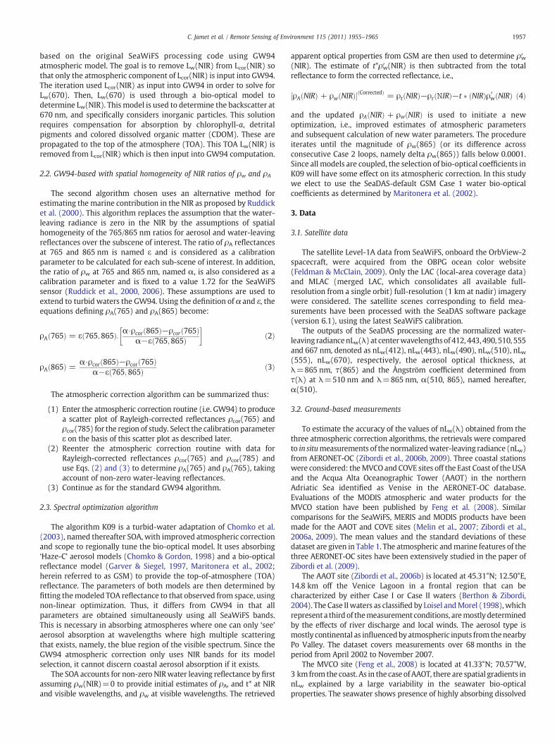
As shown by Fig. 1, by regression lines and additionally in Table 3, allalgorithms underestimate the values of nLw at all wavelengths. Thisunderestimation is less pronounced for S03. The best overall retrievals,i.e. with the lower error, are obtained with this latter algorithm withrelative error varying from 14.97% at λ=490 nm to 35.27% atλ=670 nm. The method giving the least accurate normalized water-

Table 3Statistical results for the retrieved values of nLw(λ) obtained with S03, R00 and K09.

RMS Relative error(%)

R Slope Intercept

nLw(412)S03 0.322 31.36 0.72 1.02 −0.08R00 0.360 36.81 0.68 0.85 −0.08K09 0.303 30.02 0.68 0.86 0.004

nLw(443)S03 0.318 21.81 0.81 1.00 −0.02R00 0.328 23.35 0.79 0.89 −0.02K09 0.322 24.81 0.85 0.76 0.01

nLw(490)S03 0.331 14.97 0.87 0.94 0.02R00 0.360 16.36 0.85 0.86 0.04K09 0.412 20.53 0.85 1.07 0.08

nLw(510)S03 0.357 15.13 0.85 0.90 0.03R00 0.393 17.15 0.83 0.81 0.09K09 0.340 14.54 0.82 0.89 0.14

nLw(555)S03 0.355 15.24 0.80 0.93 0.01R00 0.381 17.39 0.75 0.81 0.11K09 0.388 17.64 0.73 0.94 0.07

nLw(670)S03 0.129 35.27 0.68 0.85 −0.03R00 0.149 42.92 0.60 0.58 0.01K09 0.121 32.32 0.68 0.61 0.03

The numbers in italic represent the best statistical results.


leaving radiances is R00, the relative error being between 16.36% atλ=443 nm and 42.92% at λ=670 nm. K09 shows the best retrievals at412, 510 and 670 nm (RMS=0.303 and relative error=30.02% at412 nm, for instance) while S03 is better at λ=443, 490, 555 nm.However, none of the methods satisfies the requirements on theestimation of the nLw (Hooker et al., 1992; IOCCG, 2000), i.e. RMS~0.12for nLw(443).

The RMS can also vary as a function of the wavelength (Fig. 2). Theadvantage of S03 is that the RMS is quite constant whatever visiblewavelength is considered and thus the most stable of the threealgorithms in the comparison. Even though K09 gives the best RMSand relative error for three wavelengths, those values seem to bewavelength-dependent as the RMS vary by a factor of 1.4 between itsmaximum (at λ=490 nm) and minimum value (at λ=443 nm).

To develop bio-optical algorithms, band ratios of the water-leavingradiances are often used (O'Reilly et al., 1998). Fig. 3 presents thecomparison of the ratios nLw(443)/nLw(555), nLw(490)/nLw(555), andnLw(510)/nLw(555)obtainedwith the threemethods. Since the spectralrelative error is constant for the S03, it is of no surprise that it retrievesthe three ratios with the lowest errors. In contrast, the K09 isinconsistent across the three ratios as nLw(490)/nLw(555) is highlyoverestimated. This is anartifact of thehigher errors andRMSat 490 and555 nm (see Table 3). The algorithm R00 is the least accurate. Theseresults imply the relative effectiveness of each algorithm for use withempirical band-ratio bio-optical models. However, their drawback isthat a ‘good’ ratio could be comprised of two equally bad wavelengthcomparisons (see Table 4).

5.2. The atmospheric parameters

In addition, we present the comparison of the aerosol parametershere. Though the focus of this paper is on the nLw(λ), it is interesting,also, to look at the aerosol optical parameters as it is often done. K09does not retrieve directly the Angström exponent, α but it can beobtained through the SeaDAS software.

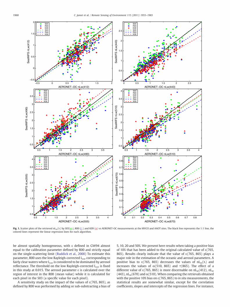
For the aerosol optical thickness τ(865) (Fig. 4, left panel), theSeaWiFS standard algorithm S03, is the most accurate algorithm andprovides the best overall estimates with an RMS of 0.033 and a relativeerror of 33% (Table 5). The least accurate algorithm is K09 with an RMSof 0.041 and a relative error of 52.25%. S03 is very accurate for the lowvalues of τ(865), but highly under-estimates the high values. K09retrieves the high values (τ(865)N0.2) with an error of 17.7% and givesretrievals that are not biased as shown by the slope (0.99) and intercept(0.02) of the linear regression. The retrievals obtainedwith S03 and R00are very similar and exhibit close values of RMS and relative errors.

From the aerosol optical thickness spectral values, the Ångströmcoefficientα(510, 865) can be calculated and estimated,whichgives thespectral dependence of τ and is a proxy of the aerosol size. None of thealgorithms is able to estimate the Ångström coefficient α(510, 865)(Fig. 4, right panel)with a high accuracy. The retrievals are relativelyflatand patchy around the 1:1 line. The best method is S03 with an RMS of0.566 and a relative error of 54.15% and the least accurate one is R00(RMS of 0.618 and relative error of 71.15%).

6. Discussion

6.1. Analysis of the retrievals errors as function of environmental factors

To understand the capabilities of each method to deal withenvironmental parameters that can affect the accuracy of retrievals ofnLw(λ), a study of the variation of the RMS and relative errors of nLw(λ)obtained with the three algorithms has been established as function ofthe turbidity, i.e. values of AERONET-OC nLw(670), the aerosol opticalthickness at 865 nm, i.e. AERONET-OC τ(865) and the level of spatial

homogeneity, i.e.σ τ 865ð Þð Þτ 865ð Þ , where σ(τ(865)) and τ 865ð Þ are the

standard deviation and mean of τ(865), respectively.No clear trends were found from the inspection of the histograms

(Fig. 5); no relations could be identified between these environmentalfactors and the retrieval errors for nLw(λ). S03 is the algorithm whichprovidesmost of the time, thebest resultswhatever factor is considered.None of the algorithms have errors correlated to either the turbidity, orto the aerosol optical thickness or to the spatial heterogeneity.

The S03 algorithm is the least sensitive to the environmental factorsas it provides themost overall accurate nLw(λ) forwhatever value of theparameters is taken into account. However, K09 canbemore accurate forspecific ranges of those factors, especially for high values of the spatialhomogeneity factor (Fig. 5). The R00 algorithm is the most sensitivemethod to the environmental factors than the two other algorithms.

6.2. Impact on the choice and estimation of the aerosol model

In order to understand the differences between the methods, it isnecessary to understand the impact of the different aerosol modelsselected by each algorithm and the way to select the aerosol model foreach pixel has to be understood. S03 and R00 differently address non-negligible NIR nLw, even if though they are both based on the GW94atmospheric correction scheme. They both partially couple the oceanand the atmosphere while K09 couples them totally.

Ahmad et al. (2010) state that the retrieved normalized water-leaving radiances values from the new set of aerosol models in S03(and GW94) were essentially the same due to the approach employedfor vicariously calibrating the water-leaving radiance retrievals, andbecause the new and old models can produce very similar spectraldependence. S03 and R00 take the same aerosol models but thehypotheses utilized for the selection of the aerosol models are quitedifferent. Both base the selection of the aerosol model on the best-fitof an aerosol parameter, ε, which represents the 765/865 nm ratio ofthe aerosol reflectance. But in R00, this parameter is consideredspatially homogeneous over the subscene of interest and has to bedetermined for each image. So the best-fit aerosol model will tend to

−0.5 0 0.5 1 1.5 2

−0.5

0

0.5

1

1.5

2

AERONET−OC nLw(412)

Sea

WiF

S n

Lw(4

12)

S03R00K09S03R00K09

0 0.5 1 1.5 2 2.50

0.5

1

1.5

2

2.5


Sea

WiF

S n

Lw(4

43)

S03R00K09S03R00K09

0.5 1 1.5 2 2.5 3 3.5

0.5

1

1.5

2

2.5

3

3.5


Sea

WiF

S n

Lw(4

90)

S03R00K09S03R00K09

0.5 1 1.5 2 2.5 3 3.5 4

0.5

1

1.5

2

2.5

3

3.5

4


Sea

WiF

S n

Lw(5

10)

S03R00K09S03R00K09

0.5 1 1.5 2 2.5 3 3.5 4

0.5

1

1.5

2

2.5

3

3.5

4


Sea

WiF

S n

Lw(5

55)

S03R00K09S03R00K09

0 0.1 0.2 0.3 0.4 0.5 0.6 0.7 0.8

0

0.1

0.2

0.3

0.4

0.5

0.6

0.7

0.8


Sea

WiF

S n

Lw(6

70)

S03R00K09S03R00K09

Fig. 1. Scatter plots of the retrieved nLw(λ) by S03( ), R00 ( ) and K09 ( ) vs AERONET-OC measurements at the MVCO and AAOT sites. The black line represents the 1:1 line, thecolored lines represent the linear regression lines for each algorithm.


be almost spatially homogeneous, with ε defined in GW94 almostequal to the calibration parameter defined by R00 and strictly equalon the single-scattering limit (Ruddick et al., 2000) To estimate thisparameter, R00 uses the low Rayleigh-corrected Lcor corresponding tofairly clear waters where Lcor is considered to be dominated by aerosolreflectance. The threshold on the low Rayleigh-corrected Lcor is fixedin this study at 0.015. The aerosol parameter ε is calculated over theregion of interest in the R00 (mean value) while it is calculated foreach pixel in the S03 (a specific value for each pixel).

A sensitivity study on the impact of the values of ε(765, 865), asdefined by R00 was performed by adding or sub-substracting a bias of

5, 10, 20 and 50%. We present here results when taking a positive biasof 10% that has been added to the original calculated value of ε(765,865). Results clearly indicate that the value of ε(765, 865) plays amajor role in the estimation of the oceanic and aerosol parameters. Apositive bias to ε(765, 865) decreases the values of nLw(λ) andincreases the values of α(510, 865) and τ(865). The effect of adifferent value of ε(765, 865) is more discernable on nLw(412), nLw(443), nLw(670) andα(510).When comparing the retrievals obtainedwith the positive 10% bias on ε(765, 865) to in situmeasurements, thestatistical results are somewhat similar, except for the correlationcoefficients, slopes and intercepts of the regression lines. For instance,

400 450 500 550 600 650 700

a b

0.1

0.15

0.2

0.25

0.3

0.35

0.4

0.45

0.5

λ(nm)

RM

SS03R00K09

400 450 500 550 600 650 70010

15

20

25

30

35

40

45

λ(nm)

RE

LAT

IVE

ER

RO

R (

%)

S03R00K09

Fig. 2. Variation of the RMS (a) and the relative error (b) as a function of the wavelength.


for nLw(443), r increases from 0.79 to 0.88, the slope increases from0.89 to 0.95. This means that the retrievals obtained with the bias onε(765, 865) are less biased than those obtained with its initial value.This trend is observed also for the aerosol optical thickness and forα(510, 865). So even with a small bias on the value of ε(765, 865), thedifferences between the twoways of estimating nLw are not negligibleand it can be assumed that these differences will increase if the bias onε(765, 865) increases.

It is also observed that R00 is not symmetricwith respect to positive/negative relative errors on ε(765, 865). In particular, if ε(765, 865) isoverestimated, thenmorepixelswill use thedefaultGW94methodwithzero nLw(NIR). However, if ε(765, 865) is underestimated, the turbidwater assumptionwill be applied tomanymore pixels. The sensitivity ofR00 to ε(765, 865) is considered a major problem for this algorithm. Asthis threshold on the low Rayleigh-corrected Lcor is determinedempirically, those values may not be fully dominated by the aerosolsand the threshold highly influences the retrievals. This is a drawback ofthe method and may explain the less accurate values of nLw(λ).

The aerosol models used in K09 are very different from those usedin the SeaWiFS standard algorithm and in R00. As explained in Section2.3, the aerosol models used in K09 have a Junge power-law size-distribution. The advantage of taking those models is that they arevery well-suited for the optimization method (only the parameter, ν,is required to describe the aerosol size distribution, compared toseveral size distribution parameters in GW94). In offshore Case Iwaters the SOA has been shown to provide good accuracy in retrievalsof apparent optical properties and hence La (Chomko et al., 2003). Sofar, results in some Case II waters are also satisfactory using K09 andreferences given earlier. This implies that for these studies, La wasretrieved to reasonable accuracy (within 5%). This does not mean thatthe size distribution (or phase function) of K09 and GW94 will agreefor similar nLw (and hence La) matchups. An aerosol model that yieldsa phase function that approximates the true phase function isrequired to retrieve accurate aerosol optical values, even for weaklyabsorbing aerosols. But, this is not the case if the goal is to retrieveonly La (see Gordon (1997) and Chomko and Gordon (1998)). Thisfactor is likely to be important in this study where the real sizedistribution is likely to be biased towards one or several models, inthis case possibly GW94. In this situation, K09 could give reasonablenLw but unreasonable τ for example.

6.3. Hypothesis on the bio-optical models

The improvements in theNIR bio-opticalmodelmade by Bailey et al.(2010) in S03 allow to decrease the number of negative normalized

water-leaving radiances in the blue (412 nm) by nearly half. Theobserved decrease in our study is 54%with our dataset (13 to 7 negativevalues).

The calibration parameter of thewater-leaving reflectance ratioα inR00 has been set to a default value of 1.72. This ratio is used to evaluatethe aerosol reflectance ρA (Eqs. 2, 3) in the NIR and its value can only beconsidered constant for weakly and moderately turbid waters while itvaries for very turbidwaters (Doron, 2007; Ruddick et al., 2006). Then ifthe value of the parameter is not exactly equal to 1.72, the incorrectestimation of the NIR ρA will occur, impact the proper choice of theaerosol model and thus lead to incorrect determination of the values ofthe water-leaving radiances in the visible channels.

The bio-optical algorithm utilized in K09, differs quite notably fromthe bio-optical model applied in the S03 and K00 (see Section 2.3).Because of the full spectrum coupled atmosphere–ocean approach ofK09, it is difficult to quantify its performance for each individualscenario. In fact, even if nLw(λ) is error free, uncertainties in thecoefficients of the bio-optical modelmay be the source of relative errorsin the retrievedbio-optical parameters (Kuchinke et al., 2009a). Becauseit is a coupled model, error in one bio-optical coefficient may actuallyinfluence retrieval of all parameters, including those relating to theatmosphere. This is particularly true if the concentration of the bio-optical parameterwhich the coefficient is related to is high (e.g., coloreddetrital material). But one advantage of this method is that no negativenLw are found in the short wavelengths. This is due to a constraint onnLwN0 applied during the optimization process.

6.4. Processing time

A comparison of the time-efficiency of the three algorithms isnecessary for operational uses. S03 couples the advantage of being thebest overall algorithm as well as being the most time-efficient. K09 isvery time-consuming as is typical of any optimization method. For thisalgorithm, smaller images were processed (0.5°-by-0.5° instead of 4°-by-4° for S03 and R00). This is amain drawback of this algorithm. R00 isalso quite efficient but less so than S03, as this method is a 2-stepalgorithmwithin the SeaDAS software. The first step is the calculation ofthe calibration parameter ε and the second step is used to perform theatmospheric correction. For series of images this first step will add timeto the processing.

7. Conclusion

In this study, a comparison is made for SeaWiFS of two algorithmsextending the “NIR black pixel” GW94 atmospheric correction

0 0.2 0.4 0.6 0.8 1

0

0.2

0.4

0.6

0.8

1

AERONET−OC nLw(443)/nLw(555)

Sea

WiF

S n

Lw(4

43)/

nLw

(555

)

S03R00K09S03R00K09

0.6 0.8 1 1.2 1.4 1.6

0.6

0.8

1

1.2

1.4

1.6


Sea

WiF

S n

Lw(4

90)/

nLw

(555

)

S03R00K09S03R00K09

0.6 0.7 0.8 0.9 1 1.1 1.2 1.3 1.4

0.6

0.7

0.8

0.9

1

1.1

1.2

1.3

1.4


Sea

WiF

S n

Lw(5

10)/

nLw

(555

)

S03R00K09S03R00K09

Fig. 3. Same as Fig. 1 but for the ratios from the left to the right: nLw(443)/nLw(555), nLw(490)/nLw(555), nLw(510)/nLw(555).

1962C.Jam

etet

al./Rem

oteSensing

ofEnvironm

ent115

(2011)1955

–1965

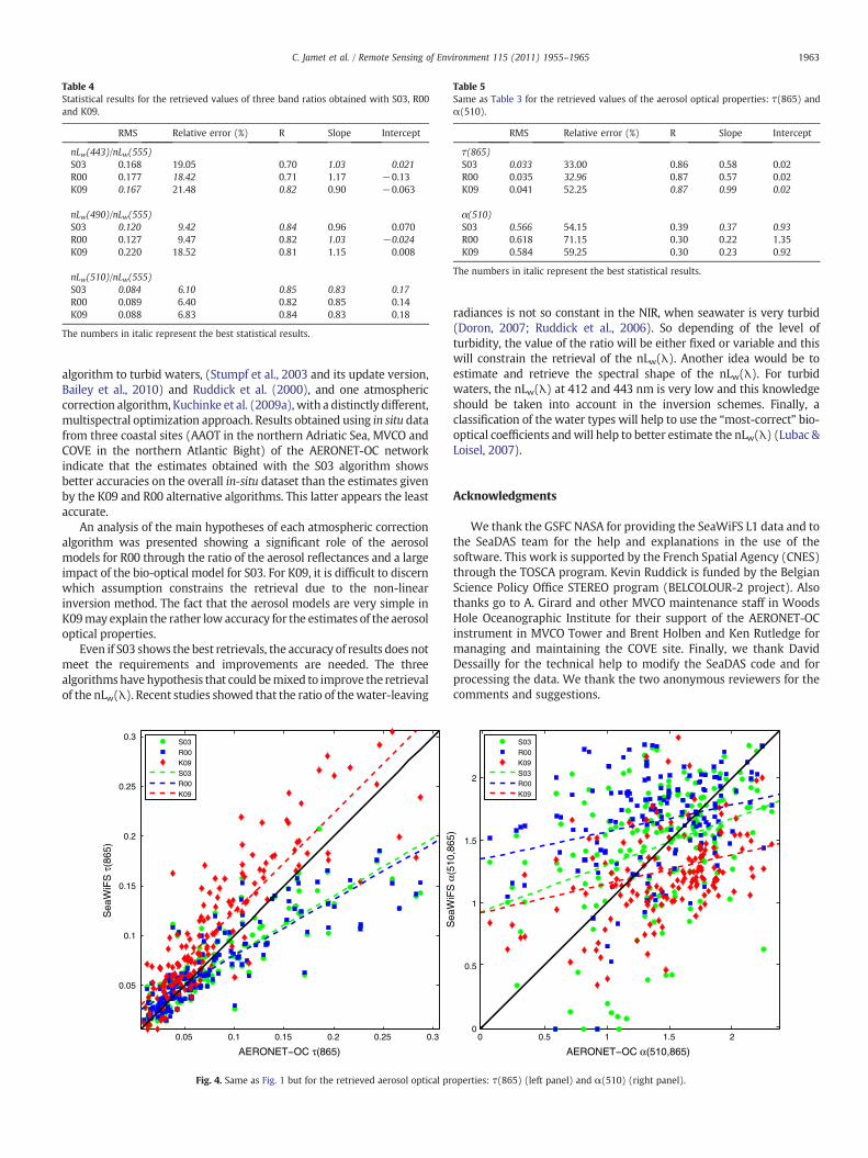
Table 5Same as Table 3 for the retrieved values of the aerosol optical properties: τ(865) andα(510).

RMS Relative error (%) R Slope Intercept

τ(865)S03 0.033 33.00 0.86 0.58 0.02R00 0.035 32.96 0.87 0.57 0.02K09 0.041 52.25 0.87 0.99 0.02

α(510)S03 0.566 54.15 0.39 0.37 0.93R00 0.618 71.15 0.30 0.22 1.35K09 0.584 59.25 0.30 0.23 0.92


Table 4Statistical results for the retrieved values of three band ratios obtained with S03, R00and K09.

RMS Relative error (%) R Slope Intercept

nLw(443)/nLw(555)S03 0.168 19.05 0.70 1.03 0.021R00 0.177 18.42 0.71 1.17 −0.13K09 0.167 21.48 0.82 0.90 −0.063

nLw(490)/nLw(555)S03 0.120 9.42 0.84 0.96 0.070R00 0.127 9.47 0.82 1.03 −0.024K09 0.220 18.52 0.81 1.15 0.008

nLw(510)/nLw(555)S03 0.084 6.10 0.85 0.83 0.17R00 0.089 6.40 0.82 0.85 0.14K09 0.088 6.83 0.84 0.83 0.18



algorithm to turbid waters, (Stumpf et al., 2003 and its update version,Bailey et al., 2010) and Ruddick et al. (2000), and one atmosphericcorrection algorithm, Kuchinke et al. (2009a), with a distinctly different,multispectral optimization approach. Results obtained using in situ datafrom three coastal sites (AAOT in the northern Adriatic Sea, MVCO andCOVE in the northern Atlantic Bight) of the AERONET-OC networkindicate that the estimates obtained with the S03 algorithm showsbetter accuracies on the overall in-situ dataset than the estimates givenby the K09 and R00 alternative algorithms. This latter appears the leastaccurate.

An analysis of the main hypotheses of each atmospheric correctionalgorithm was presented showing a significant role of the aerosolmodels for R00 through the ratio of the aerosol reflectances and a largeimpact of the bio-optical model for S03. For K09, it is difficult to discernwhich assumption constrains the retrieval due to the non-linearinversion method. The fact that the aerosol models are very simple inK09may explain the rather low accuracy for the estimates of the aerosoloptical properties.

Even if S03 shows the best retrievals, the accuracy of results does notmeet the requirements and improvements are needed. The threealgorithmshavehypothesis that could bemixed to improve the retrievalof the nLw(λ). Recent studies showed that the ratio of thewater-leaving

0.05 0.1 0.15 0.2 0.25 0.3

0.05

0.1

0.15

0.2

0.25

0.3

AERONET−OC τ(865)

Sea

WiF

S τ

(865

)

S03R00K09S03R00K09

Fig. 4. Same as Fig. 1 but for the retrieved aerosol optical pr

radiances is not so constant in the NIR, when seawater is very turbid(Doron, 2007; Ruddick et al., 2006). So depending of the level ofturbidity, the value of the ratio will be either fixed or variable and thiswill constrain the retrieval of the nLw(λ). Another idea would be toestimate and retrieve the spectral shape of the nLw(λ). For turbidwaters, the nLw(λ) at 412 and 443 nm is very low and this knowledgeshould be taken into account in the inversion schemes. Finally, aclassification of the water types will help to use the “most-correct” bio-optical coefficients andwill help to better estimate the nLw(λ) (Lubac &Loisel, 2007).

Acknowledgments

We thank the GSFC NASA for providing the SeaWiFS L1 data and tothe SeaDAS team for the help and explanations in the use of thesoftware. This work is supported by the French Spatial Agency (CNES)through the TOSCA program. Kevin Ruddick is funded by the BelgianScience Policy Office STEREO program (BELCOLOUR-2 project). Alsothanks go to A. Girard and other MVCO maintenance staff in WoodsHole Oceanographic Institute for their support of the AERONET-OCinstrument in MVCO Tower and Brent Holben and Ken Rutledge formanaging and maintaining the COVE site. Finally, we thank DavidDessailly for the technical help to modify the SeaDAS code and forprocessing the data. We thank the two anonymous reviewers for thecomments and suggestions.

0 0.5 1 1.5 20

0.5

1

1.5

2

AERONET−OC α(510,865)

Sea

WiF

S α

(510

,865

)

S03R00K09S03R00K09

operties: τ(865) (left panel) and α(510) (right panel).

0.1 0.2 0.3 0.4 0.5 0.6 0.7 0.80

10

20

30

40

50

60

70

80

nLw(670)

Rel

ativ

e er

ror

(%)

on S

eaW

iFS

nL w

(412

)

Rel

ativ

e er

ror

(%)

on S

eaW

iFS

nL w

(412

)

Rel

ativ

e er

ror

(%)

on S

eaW

iFS

nL w

(412

)

S03R00K09

0 0.05 0.1 0.15 0.2 0.25 0.3 0.350

10

20

30

40

50

60

70

80

AERONET−OC τ(865)

S03R00K09

0.02 0.04 0.06 0.08 0.1 0.12 0.14 0.16 0.18 0.20

5

10

15

20

25

30

35

40

45

50

Spatial heterogeneity

S03R00K09

a b

c

Fig. 5. Variation of the relative error on nLw(412) as a function of the values of (top to bottom): (i) nLw(670) (e.g., turbidity), (ii) τ(865) and (iii) the spatial homogeneity.


References

Ahmad, Z., Franz, B. A., McClain, C. R., Kwiatkowska, E. J., Werdell, J., Shettle, E. P., et al.(2010). New aerosol models for the retrieval of aerosol optical thickness andnormalized water-leaving radiances from the SeaWiFS and MODIS sensors overcoastal regions and open oceans. Applied Optics, 49, 5545−5560.

Bailey, S., & Wang, M. (2001). Satellite aerosol optical thickness match-up procedures.NASA technical memorandum, 2001-209982 (pp. 70−72). Greenbelt, MD: NASAGoddard Space Flight Center.

Bailey, S.W., Franz, B. A., &Werdell, P. J. (2010). Estimation of near-infraredwater-leavingreflectance for satellite ocean color data processing. Optics Express, 18, 7521−7527.

Baith, K., Lindsay, R., Fu, G., & McClain, C. R. (2001). SeaDAS, a data analysissystem forocean-color satellite sensors. Eos Transactions AGU, 82, 202.

Banzon, V. F., Gordon, H. R., Kuchinke, C. P., Antoine, D., Voss, K. J., & Evans, R. H. (2009).Validation of SeaWiFS dut-correction methodology in the Mediterranean Sea:Identification of an algorithm-switching criterion. Remote Sensing of Environment, 113,2689−2700.

Berthon, J. -F., & Zibordi, G. (2004). Bio-optical relationships for the northern AdriaticSea. International Journal of Remote Sensing, 25, 1527−1532.

Chomko, R. M., & Gordon, H. R. (1998). Atmospheric correction of ocean color imagery:Use of the Junge power-law aerosol size distribution with variable refractive indexto handle aerosol absoprition. Applied Optics, 37, 5560−5572.

Chomko, R. M., Gordon, H. R., Maritonera, S., & Siegel, D. A. (2003). Simultaneousretrieval of oceanic and atmospheric parameters for ocean color imagery byspectral optimization: A validation. Remote Sensing of Environment, 84, 202−220.

Doron,M. (2007). Utilisation des données de couleur de l'océan pour estimer les propriétésoptiques des eaux côtières: Caractérisation du signal marin dans le proche infrarougepour les eaux turbides, développementd'algorithmes semi-analytiques, validation avecdes données satellitaires, PhD dissertation, Université Pierre et Marie Curie, 183 pp.

Feldman, G. C., & McClain, C. R. (2009). In N. Kuring, & S. W. Bailey (Eds.), Ocean colorweb, SeaWiFS reprocessing 2009. : NASA Goddard Space Flight Centerhttp://www.oceancolor.gsfc.nasa.gov/.

Feng, H., Vandemark, D., Campbell, J. W., & Holben, B. N. (2008). Evaluation of MODISocean color products at a northeast United States coast site near the Martha'sVineyard Coastal Observatory. International Journal of Remote Sensing, 29,4479−4497.

Fu, G., Baith, K. S., & McClain, C. R. (1998). SeaDAS: The SeaWiFS data analysis system.Proceedings of the 4th Pacific Ocean remote sensing conference, Qingdao, China, July28–31 (pp. 73−79).

Garver, S., & Siegel, D. A. (1997). Inherent optical property inversion of ocean colorspectra and its biogeochemical interpretation: 1 time series from the Sargasso Sea.Journal of Geophysical Research, 102, 18607−18625.

Gordon, H. R. (1997). Atmospheric correction of ocean color imagery in the EarthObserving System era. Journal of Geophysical Research, 102, 17081−17106.

Gordon, H. R., & Wang, M. (1994). Retrieval of water-leaving radiance and aerosoloptical thickness over the oceans with SeaWiFS: A preliminary algorithm. AppliedOptics, 33, 443−452.

Gould, R. W., Arnone, R. A., & Sydor, M. (1998). Testing a new remote sensingreflectance algorithm to estimate absorption and scattering in case-2 waters. SPIEOcean Optics XII, Hawaï, USA.

Hess, M., Koepke, P. L., & Schult, I. (1998). Optical properties of aerosols and clouds: Thesoftware package OPAC. Bulletin of the American Meteorological Society, 79, 831−844.

Hooker, S. B., Esaias, W. E., Feldman, G. C., Gregg, W. W., & McClain, C. R. (1992). Anoverview of SeaWiFS and ocean color. In S. B. Hooker, & E. R. Firestone (Eds.), NASATech Memo. 104566, Vol. 1, Greenbelt, Maryland: NASA Goddard Space Flight Center24 pp.

Hu, C., Carder, K. L., & Muller-Karger, F. E. (2000). Atmospheric correction of SeaWiFSimagery over turbid coastal waters. Remote Sensing of Environment, 74, 195−206.

IOCCG (2000). Remote sensing of ocean colour in coastal, and other optically-complex,waters. In S. Sathyendranath (Ed.), Reports of the International Ocean-ColourCoordinating Group, No. 3 (pp. 140). Darmouth, Canada: IOCCG.

IOCCG (2010). Atmospheric correction for remotely-sensed ocean-colour products. InM. H.Wang (Ed.), Reports of the international ocean-colour coordinating group, no. 10(pp. 78). Darmouth, Canada: IOCCG.

http://www.oceancolor.gsfc.nasa.gov/

http://www.oceancolor.gsfc.nasa.gov/


Kuchinke, C. P., Gordon, H. R., & Franz, B. A. (2009a). Spectral optimization forconstituent retrieval in Case II waters I: Implementation and performance. RemoteSensing of Environment, 13, 571−587.

Kuchinke, C. P., Gordon, H. R., Harding, L. W., Jr., & Voss, K. J. (2009b). Spectraloptimization for constituent retrieval in Case II waters II: Validation study in theChesapeake Bay. Remote Sensing of Environment, 113, 610−621.

Land, P. E., & Haigh, J. D. (1996). Atmospheric correction over case 2 waters with aniterative fitting algorithm. Applied Optics, 35, 5443−5451.

Lavender, S. J., Pinkerton, M. H., Moore, G. F., Aiken, J., & Blondeau-Patissier, D. (2005).Modification to the atmospheric correction of SeaWiFS ocean colour images overturbid waters. Continental Shelf Research, 25, 539−555.

Loisel, H., & Morel, A. (1998). Light scattering and chlorophyll concentration in case 1waters: A reexamination. Limnology and Oceanography, 43, 847−858.

Lubac, B., & Loisel, H. (2007). Variability and classification of remote sensing reflectancespectra in the eastern English Channel and southern North Sea. Remote Sensing ofEnvironment, 110, 45−58.

Maritonera, S., Siegel, D. A., & Peterson, A. R. (2002). Optimization of semianalyticalocean color model for global scale applications. Applied Optics, 41, 2705−2714.

Melin, F., Zibordi, G., & Berthon, J. -F. (2007). Assessment of satellite ocean colorproducts at a coastal site. Remote Sensing of Environment, 110, 192−215.

Morel, A., & Prieur, L. (1977). Analysis of variations in ocean color. Limnology andOceanography, 22, 709−722.

O'Reilly, J. E., Maritonera, S., Michell, B. G., Siegel, D. A., Carder, K. L., Garver, S. A., Kahru,M., & McClain, C. (1998). Ocean color chlorophyll algorithms for SeaWiFS. Journal ofGeophysical Research, 103, 24937−24953.

Oo, M., Vargas, M., Gilerson, A., Gross, B., Moshary, F., & Ahmed, S. (2008). Improvingatmospheric correction for highly productive coastal waters using the short waveinfrared retrieval algorithm with water-leaving reflectance constraints at 412 nm.Applied Optics, 47, 3846−3859.

Ransibrahmanakul, V., Stumpf, R., Ramachandran, S., & Hughes, K. (2005). Evaluation ofatmospheric correction algorithm for processing SeaWiFS data. Proceeding SPIE,5885, doi:10.1117/12.615722.

Robinson, W. D., Franz, B. A., Patt, F. S., Bailey, S. W., & Werdell, P. J. (2003). Masks andflags updates. In S. B. Hooker, & E. R. Firestone (Eds.), SeaWiFS Postlaunch TechnicalReport Series, Chap.6, NASA/TM-2003-206892, Vol. 22. (pp. 34−40).

Ruddick, K. G., De Cauwer, V., Park, Y. -J., & Mooe, G. (2006). Seaborne measurements ofnear infrared water-leaving reflectance: The similarity spectrum for turbid waters.Limnology and Oceanography, 51, 1167−1179.

Ruddick, K. G., Ovidio, F., & Rijkeboer, M. (2000). Atmospheric correction of SeaWiFSimagery for turbid coastal and inland waters. Applied Optics, 39, 897−912.

Shanmugam, P., & Ahn, Y. H. (2007). New atmospheric correction technique to retrievethe ocean colour from SeaWiFS imagery in complex coastal waters. Journal of OpticsA: Pure and Applied Optics, 9, 511−530.

Siegel, D. A., Wang, M., Maritonera, S., & Robinson, W. (2000). Atmospheric correction ofsatellite oceancolor imagery: Theblackpixel assumption.AppliedOptics,39, 3582−3591.

Stumpf, R. P., Arnone, R. A., Gould, R. W., & Ransibrahmanakul, V. (2003). A partlycoupled ocean–atmosphere model for retrieval of water-leaving radiance fromSeaWiFS in coastal waters. NASA technical memorandum 2003-206892(22)(pp. 51−59). Greenbelt, MD: NASA Goddard Space Flight Center.

Zibordi, G., Holben, B., Hooker, S. B., Melin, F., Berthon, J. -F., Slutsker, I., Giles, D.,Vandemark, D., Feng, D., Rutledge, K., Schuster, G., & Al Mandoos, A. (2006). Anetwork for standardized ocean color validation measurements. EOS Transactions,87, 293−297.

Zibordi, G., Holben, B., Slutsker, I., Giles, D., D'Alimonte, D., Mélin, F., Berthon, J. -F.,Vandemark, D., Feng, H., Schuster, G., Fabbri, B. E., Kaitala, S., & Seppälä, J. (2009).AERONET-OC: A network for the validation of ocean color primary products. Journalof Atmospheric and Oceanic Technology, 26, 1634−1651.

Zibordi, G., Melin, F., & Berthon, J. -F. (2006). Comparison of SeaWiFS, MODIS andMERIS radiometric products at a coastal site. Geophysical Research Letters, 33,L06617, doi:10/1029/2006GL025778.

http://dx.doi.org/10.1117/12.615722

http://dx.doi.org/10/1029/2006GL025778

remote sensing of environment - vliz · comparison of three seawifs atmospheric correction...

Documents