robust spectroscopic quantification in turbid...
TRANSCRIPT
Robust spectroscopic quantification in turbid media.
Francis W.L. Esmonde-White
Ph.D. Thesis
Department of Chemistry
McGill University
Montreal, Quebec, Canada
Dec. 01, 2008
A thesis submitted to McGill University in partial fulfilment of the
requirements of the degree of Doctor of Philosophy
Francis W.L. Esmonde-White, 2008.

ii
Dedication
This thesis is dedicated to: my wife, Karen, whose emotional
support and scientific advice has been invaluable; my brothers, Emmett
and Steve, without whom the world would have been much less colourful;
and my parents, who instilled in me curiosity and perseverance.
iii
Abstract
This thesis explores four methods for improving quantitative diffuse
reflectance spectroscopy in light scattering media. To begin, an
introduction is given outlining theories of light propagation in scattering
media, relevant instrumentation for measuring light scattering properties,
spectral data processing methods, and spectroscopically active
bioanalytes. Four novel contributions to science are made. Each is
described in a chapter. The improvements consist of two novel
instruments for practical scattering measurements, and two novel data
processing techniques. Finally, directions for future research into diffuse
reflectance spectroscopy are suggested.
A novel photon time-of-flight device is first presented. This portable
instrument is used to measure scattering coefficients in tandem with a
portable diode spectrometer. The measured scattering coefficients are
then used to correct the co-measured near infrared spectra for scattering
and for improving quantification. Reduced scattering coefficients were
measured with coefficients of variation of 11.6% at 850 nm and 14.1% at
905 nm. This simplified photon time-of-flight instrument allows for practical
correction of light scattering in point-spectra. Using scattering-correction,
estimates of dye concentration were improved by 35%. Applications
iv
include integration with handheld spectrometers for development of
handheld near-infrared medical diagnostic equipment.
A novel device for imaging annular patterns is presented. This
imaging instrument is used to measure reduced scattering coefficients and
absorption coefficients. This simple imaging system measures the optical
properties using small source-detector spacings, resulting in high spatial
resolution. Potential applications include correction of imaging
spectroscopy in surgery and clinical applications. Reduced scattering
coefficients were measured with a coefficient of variation of 12.6%, and
absorption coefficients were measured with a coefficient of variation 50%
lower than using traditional imaging methods.
A novel method for using parsimony in the development of data
processing methods using genetic algorithms is presented. Genetic
algorithms have been used to identify spectroscopic data processing
methods for complex samples. A problem in the automated identification
of processing models is that genetic algorithms tend to select
unnecessarily complex models, which may fit noise. Parsimony methods
are used to guide the selection process towards smaller models. Previous
works have typically used custom parsimony penalty functions. Rather
than custom penalties appropriate for particular data sets, a method using
v
penalization based on the number of incorporated wavelengths or pre-
processing options was developed. This technique has applicability in the
development of future spectrometric hardware, particularly for the
development of simplified multiwavelength probes. Using the
parsimonious genetic algorithm, a data processing model was found for
estimating lactate concentration in tissue with a 41% improvement in
standard error as compared to the best expert developed model.
A novel method is presented using multivariate curve resolution to
measure myoglobin oxygen saturation from diffuse reflectance spectra of
cardiac tissue. Multivariate curve resolution algorithms are used to
simultaneously estimate the pure component profiles and the relative
component weightings directly from recorded data. Changes in spectral
shape due to scattering and the local chemical environment are modeled
using multivariate curve resolution to estimate the hemoglobin and
myoglobin component spectra from the recorded data. Oxygen saturation
estimates using the multivariate curve resolution algorithm were compared
to oxygen saturation estimates using a classical least squares approach.
Multivariate curve resolution estimated myoglobin oxygen saturation better
than the classical least squares method. Simulations also show that
spectral data spanning the upper 15% oxygen saturation range should
vi
allow for estimates of myoglobin oxygen saturation using multivariate
curve resolution. The multivariate curve resolution algorithm was tested
with spectra of guinea pig hearts perfused with blood, and showed a 100%
improvement in accuracy as compared to the classical least squares
approach.
The four methods developed in this thesis each showed
improvement in the quantification of components using diffuse reflectance
spectra. The photon time-of-flight and genetic algorithm methods are
particularly applicable in point-measurements, and in the development of
simplified portable instrumentation. The annular-beam imaging and
multivariate curve resolution methods have use in spectral imaging for
mapping chemical properties across a surface. Further applications and
suggestions for future work are given in the conclusions chapter.
vii
Résumé
Cette thèse explore quatre méthodes pour l'amélioration de la
spectroscopie de réflectance diffuse quantitative dans des milieux qui
diffusent la lumière. En introduction, une description des théories de la
propagation de la lumière dans des médias qui diffusent celle-ci, des
instruments pour mesurer les propriétés de diffusion, des méthodes de
traitement des données spectrales, et des bioanalytes avec activité
optique est donné. Quatre contributions à la science (une par chapitre)
sont décrites. Les améliorations sont composées de deux nouveaux
instruments facilitant la mesure de la dispersion, et de deux nouvelles
techniques de traitement des données. Enfin, plusieurs perspectives sur la
spectroscopie de réflectance diffuse sont suggérées.
Un nouvel appareil à «temps de vol de photon» est présenté. Cet
instrument portatif est utilisé pour mesurer le coefficient de dispersion en
tandem avec un spectromètre à diode portable. Les coefficients de
diffusion mesurés sont ensuite utilisés pour corriger la dispersion dans les
spectres infrarouges co-mesurée, ainsi que l'amélioration de la
quantification. Les coefficients de dispersion ont été mesurés avec une
variation de 11,6% à 850 nm et 14,1% à 905 nm. Cette approche
simplifiée par un instrument à «temps de vol de photon» permet une
viii
approche pratique pour la correction de la diffusion de la lumière dans les
spectres. En prenant en compte la dispersion, les estimations de la
concentration de teinture ont été améliorées de 35%. Les applications
incluent l'intégration avec des spectromètres portatifs pour créer de
nouveau équipement pour diagnostiques médicaux.
Un nouvel appareil utilisant les modes d'imagerie annulaire est
présenté. Cet instrument est utilisé pour mesurer les coefficients de
dispersion et d'absorption. Ce système d'imagerie optique simple mesure
les propriétés de dispersion et absorption de la lumière à l'aide de petits
espacements entre la source et le détecteur, conduisant à une haute
résolution spatiale. Les applications potentielles incluent la correction de
l'imagerie spectroscopique dans l'application clinique. Les coefficients de
dispersion ont été mesurés avec un coefficient de variation de 12,6%, et
les coefficients d'absorption ont été mesurés avec un coefficient de
variation amélioré de 50% par rapport aux méthodes d'imagerie
traditionnelle.
Une nouvelle méthode pour améliorer l'utilisation des mesures de
simplicité dans le développement de méthodes de traitement des données
via des algorithmes génétiques est présentée. Les algorithmes génétiques
ont été utilisés pour identifier les méthodes de traitement de données
ix
spectroscopiques pour des échantillons complexes. Un problème dans le
traitement automatisé d'identification des modèles est que les algorithmes
génétiques ont tendance à sélectionner les modèles complexe inutile, qui
peuvent par exemple correspondre le bruit de fond. Des mesures de
simplicité sont utilisées pour guider le processus de sélection vers des
modèles plus petits. Les travaux précédant ont généralement utilisé des
fonctions faite sur mesure. Plutôt que ces fonctions fait sur mesure, des
sanctions appropriés pour différentes séries de données ont été élaboré
en utilisant une méthode fondée sur la pénalisation du nombre d'ondes ou
incorporés «pre-processing options» inclus. Cette technique est applicable
dans le développement de nouvelles méthodes spectroscopiques, en
particulier pour le développement des nouveaux appareils simplifiés. Un
modèle de traitement des données a été déterminé par l'utilisation de
l'algorithme génétique parcimonieuse pour l'estimation de la concentration
de lactate avec une amélioration de 41% de la marge d'erreur standard
par rapport au meilleur modèle d'expertise déjà développe.
Une nouvelle méthode a été développée en utilisant la
«multivariate curve resolution» pour mesurer la saturation en oxygène de
la myoglobine par spectres réflexion diffuse des tissus cardiaques. Les
algorithmes «multivariate curve resolution» sont utilisés pour estimer
x
simultanément les profils de corps pur et de la composante relative
directement à partir des données enregistres. Les changements de forme
spectrale en raison de la diffraction et de l'environnement chimique local
sont modélisés en utilisant la «multivariate curve resolution» pour estimer
le taux d'hémoglobine et de myoglobine dans les échantillons. La
saturation de l'oxygène mesurée en utilisant le «multivariate curve
resolution» a été comparées aux estimations de la saturation de l'oxygène
au moyen d'une approche classique des moindres carrés. «Multivariate
curve resolution» a estimée la saturation d'oxygène en myoglobine
supérieure à la méthode classique des moindres carrés.
Les simulations montrent également que les données spectrales
couvrant la partie supérieure de la saturation en oxygène de 15%
devraient permettre des estimations de la myoglobine saturation de
l'oxygène en utilisant la courbe de résolution multivariée. La algorithme
«multivariate curve resolution» a été testé avec des spectres de cœurs
Cochon d'Inde perfusés avec du sang, et a montré une amélioration de
100% par rapport à la précision de la méthode classique des moindres
carrés.
Les quatre méthodes développées dans cette thèse ont montré
l'amélioration de quantification avec la spectroscopie de réflectance
xi
diffuse. L'appareil à «temps de vol de photon» et l'algorithme génétique
sont notamment applicables aux mesures poindre, pour le développement
de simples appareils portatif pour diagnostiques médicaux. Les méthodes
d'imagerie de la lumière annulaire et la «multivariate curve resolution» ont
recours à l'imagerie spectrale pour la cartographie des propriétés
chimiques à travers d'une surface. D'autres demandes et des suggestions
pour les travaux futurs sont présentées dans le chapitre consacré aux
conclusions.
xii
Table of Contents
Dedication ............................................................................................................................ii
Abstract ............................................................................................................................... iii
Résumé .............................................................................................................................. vii
Table of Contents ............................................................................................................... xii
List of Figures .................................................................................................................... xvi
List of Tables ................................................................................................................... xviii
List of Commonly Used Symbols ...................................................................................... xix
Original Contributions to Knowledge ..................................................................................xx
Contribution of Authors ..................................................................................................... xxi
Copyright Waivers ............................................................................................................ xxv
Chapter 1. Research Objectives and Overview ................................................................ 28
1.1 Research Objectives .............................................................................................. 30
1.2 Project Overview and Thesis Layout ...................................................................... 31
Chapter 2. ......................................................................................................................... 37
Introduction to Spectroscopy in Turbid Media .................................................................. 37
2.1 Overview and Theory of Light Scattering ............................................................... 39
2.1.1 Radiative Transport Equation and the Diffusion Approximation ..................... 42
2.2 Instrumentation for Measuring Scattering .............................................................. 45
2.2.1 Steady-State Instruments ................................................................................ 45
2.2.2 Time-Resolved Instruments ............................................................................ 47
2.3 Data Processing for Quantitative Spectroscopy in Scattering Media ..................... 53
2.3.1 Quantification from Measured Spectra ............................................................ 54
2.3.1.1 Ratiometric Probes and Simple Imaging ................................................. 55
2.3.1.2 Processing Full Spectra without Measured Scattering ............................ 56
2.3.2 Quantification from Optical Properties Measurements.................................... 58
2.3.3 Quantification from Spectra and Optical Properties Measurements ............... 59
2.3.3.1 Using One Recorded Spectrum and Diffusion Model Estimation ............ 59
2.3.3.2 Using Many Recorded Spectra ................................................................ 60
2.4 Tissue Properties and Spectroscopically Active Bioanalytes ................................. 61
2.4.1 Window for Spectroscopic Analysis of Tissue ................................................. 62
2.4.2 Optical Properties of Tissues .......................................................................... 64
2.4.3 Overview of Spectrally Active Respiratory Metabolic Processes .................... 65
2.4.4 Hemoglobin Oxygen Saturation Measurement ............................................... 70
2.4.5 Myoglobin Oxygen Saturation Measurement .................................................. 73
2.4.6 Carbohydrate and Other Spectral Features .................................................... 75
xiii
Chapter 3. A Portable Multi-Wavelength Near-Infrared Photon Time-of-Flight Instrument
for Measuring Light Scattering .......................................................................................... 78
3.1 Manuscript .............................................................................................................. 80
3.2 Abstract ................................................................................................................... 80
3.3 Keywords ................................................................................................................ 81
3.4 Introduction ............................................................................................................. 81
3.5 Method .................................................................................................................... 85
3.5.1 Temporal Measurements ................................................................................ 86
3.5.2 Software Processing ....................................................................................... 90
3.5.3 Spectroscopic Measurements ......................................................................... 91
3.5.4 Optical Probe ................................................................................................... 91
3.6 Materials ................................................................................................................. 92
3.7 Results & Discussion .............................................................................................. 95
3.8 Conclusions .......................................................................................................... 103
3.9 Acknowledgements .............................................................................................. 104
Chapter 4. Steady-State Diffuse Reflectance Imaging of an Annular Source Illumination
Pattern for Quantifying Scattering and Absorption Coefficients of Turbid Media ........... 106
4.1 Manuscript ............................................................................................................ 108
4.2 Abstract ................................................................................................................. 108
4.3 Keywords .............................................................................................................. 109
4.4 Introduction ........................................................................................................... 109
4.5 Material and Methods ........................................................................................... 113
4.5.1 Instrument Configuration ............................................................................... 113
4.5.2 Software ........................................................................................................ 117
4.5.3 Phantom Tissue Samples ............................................................................. 117
4.6 Results and Discussion ........................................................................................ 118
4.6.1 Estimation of Reduced Scattering Coefficient ............................................... 122
4.6.2 Estimation of Absorption Coefficient ............................................................. 125
4.7 Conclusion ............................................................................................................ 130
4.8 Acknowledgements .............................................................................................. 132
Chapter 5. Generic Parsimony in Genetic Algorithms for Selecting Spectral Processing
Models in Regression and Classification ........................................................................ 133
5.1 Genetic Algorithms ............................................................................................... 134
5.2 Manuscript ............................................................................................................ 136
5.3 Abstract ................................................................................................................. 136
5.4 Keywords .............................................................................................................. 137
5.5 Introduction ........................................................................................................... 138

xiv
5.6 Methodology ......................................................................................................... 141
5.6.1 Software ........................................................................................................ 142
5.6.2 Pre-processing Options and Score Calculation ............................................ 144
5.6.3 Binary Representation of Processing Models ............................................... 145
5.6.4 Regression Fitness Function ......................................................................... 146
5.6.5 Classification Fitness Function ...................................................................... 148
5.6.6 Selection of Models ....................................................................................... 152
5.7 Test Data .............................................................................................................. 154
5.7.1 Regression Data Set ..................................................................................... 154
5.7.2 Classification Data Set .................................................................................. 155
5.8 Results and Discussion ........................................................................................ 156
5.8.1 Regression Model Development ................................................................... 157
5.8.2 Development of Classification Models .......................................................... 163
5.9 Conclusions .......................................................................................................... 169
5.10 Acknowledgements ............................................................................................ 170
Chapter 6. Estimation of Myoglobin Oxygen Saturation from Spectra of Cardiac Tissue
using Multivariate Curve Resolution ............................................................................... 172
6.1 Multivariate Curve Resolution ............................................................................... 173
6.2 Manuscript ............................................................................................................ 176
6.3 Abstract ................................................................................................................. 176
6.4 Keywords .............................................................................................................. 177
6.5 Introduction ........................................................................................................... 177
6.6 Theory ................................................................................................................... 182
6.7 Experimental ......................................................................................................... 189
6.7.1 Simulated Data .............................................................................................. 189
6.7.2 Cardiac Tissue Data ...................................................................................... 191
6.8 Results & Discussion ............................................................................................ 192
6.8.1 Simulated Tissue Measurements .................................................................. 193
6.8.2 Measurements of Guinea Pig Hearts ............................................................ 200
6.9 Conclusions .......................................................................................................... 204
Chapter 7. Conclusions and Future Work ....................................................................... 206
7.1 Conclusions .......................................................................................................... 207
7.2 Future Work .......................................................................................................... 211
7.2.1 Future Work using the Photon Time-of-Flight Instrument ............................. 211
7.2.2 Future Work using the Ring-Light System .................................................... 215
7.2.3 Future Work using the Genetic Algorithm ..................................................... 217
7.2.3 Future Work using Multivariate Curve Resolution ......................................... 218
xv
7.3 Conclusion ............................................................................................................ 220
Appendix A: TOF Device................................................................................................. 221
A.1 Time-of-Flight Control Electronics Schematic ...................................................... 222
A.2 Time-of-Flight Control Electronics Part List ......................................................... 223
A.3 Photon Time-of-Flight Electronic Control System C Code ................................... 227
A.4 Mellin Transform for Estimating Statistical Moments ........................................... 237
Appendix B: Ring-Light Device ....................................................................................... 239
Appendix C: Genetic Algorithm Code ............................................................................. 243
Appendix D: MCR Code .................................................................................................. 255
Appendix E: N-Way Visualization Manuscript Reprint .................................................... 259
Appendix F: Tissue Simulating Phantoms ...................................................................... 266
Appendix G: Numerical Models of Light Scattering ........................................................ 269
G.1 Finite Element Analysis ....................................................................................... 269
G.2 Monte Carlo Simulations ...................................................................................... 270
Bibliography .................................................................................................................... 273
xvi
List of Figures
Figure 2.1: Light transport in scattering media ................................................................. 39
Figure 2.2: Principle of similarity ....................................................................................... 42
Figure 2.3: Example of a bench scale photon time-of-flight instrument ............................ 47
Figure 2.4: The therapeutic window .................................................................................. 62
Figure 2.5: A simplified diagram of aerobic and anaerobic respiration ............................. 65
Figure 2.6: NIR spectra of hemoglobin, myoglobin, cyt. c, and cyt. oxidase .................... 69
Figure 2.7: NIR spectra of lactate and glucose. ................................................................ 77
Figure 3.1: Instrument configuration schematic with inset probe diagram. ...................... 86
Figure 3.2: Laser controller circuit schematic ................................................................... 89
Figure 3.3: Scattering intensity with reduced scattering coefficient .................................. 94
Figure 3.4: Trends in the recorded laser pulse profiles .................................................... 96
Figure 3.5: Regression plots showing μs' estimation ........................................................ 99
Figure 3.6: Dye concentration estimates with scattering correction ............................... 101
Figure 4.1: Instrumental configuration for annular pattern imaging ................................ 114
Figure 4.2: Computer generated holographic interference filter. .................................... 115
Figure 4.3: Images of the four annular patterns .............................................................. 120
Figure 4.4: Radial reflectance intensity profiles of ring illumination ................................ 121
Figure 4.5: Scattering calibration and validation ............................................................. 122
Figure 4.6: Polynomial curve approximation of the reflectance intensity ........................ 126
Figure 4.7: Absorption coefficient estimation from integrated reflectance intensity ....... 128
Figure 5.1: Bitstring representation diagram ................................................................... 146
Figure 5.2: Models for determining lactate concentration ............................................... 156
Figure 5.3: Pre-processed NIR spectra for lactate estimation ........................................ 160
Figure 5.4: Lactate estimations ....................................................................................... 162
Figure 5.5: Models for classification of starches ............................................................. 164
Figure 5.6: Pre-processed starch spectral data .............................................................. 165
Figure 5.7: Gaussian functions fitted to the score values ............................................... 167
Figure 5.8: Bayesian class estimates ............................................................................. 169
Figure 6.1: Spectra estimated from MCR processing of simulated tissue spectra ......... 194
Figure 6.2: Calibration plots comparing tissue oxygen saturation estimates .................. 195
Figure 6.3: Simulated tissue processing validation results ............................................. 199
Figure 6.4: Myoglobin composition estimate from MCR ................................................. 202
Figure 6.5: Spectral profiles estimated for first guinea pig heart ................................... 204
Figure 7.1: Improvements to the photon time-of-flight: preliminary results. .................... 213
Figure A.1: Schematic for the Time-of-Flight electronic control board. .......................... 222

xvii
Figure A.2: Printed circuit board layout for the Time-of-Flight electronic control board . 225
Figure A.3: Printed circuit board tracesfor the Time-of-Flight electronic control board .. 226
Figure G.1: Example results from a Monte Carlo simulation. ......................................... 271

xviii
List of Tables
Table 2.1: Measured optical properties of human tissue ................................................. 64
Table 3.1: Regression estimations of reduced scattering coefficients .............................. 98
Table 5.1: Classification parsimony functions ................................................................. 151
Table 6.1: Residual error and linearity estimations of oxygen saturation ...................... 190
Table 6.2: Myoglobin oxygen saturation at the experimental saturation endpoints ....... 200

xix
List of Commonly Used Symbols
μs – scattering coefficient (typically in mm-1 or cm-1)
μs' – reduced scattering coefficient (typically in mm-1 or cm-1)
μa – absorption coefficient (typically in mm-1 or cm-1)
g – anisotropy
I – intensity
I0 – absorption-free reference intensity
g – anisotropy
ε – molar absorptivity
c – concentration
L – pathlength
A – absorption or attenuation

xx
Original Contributions to Knowledge
1. Development of a portable, hand-held photon time-of-flight instrument
to measure optical scattering properties and improve near infrared
reflectance quantification of scattering media.
2. Development of a novel diffuse reflectance imaging system using a
ring-patterned laser to estimate optical scattering and absorption
properties of scattering media with high spatial resolution.
3. Development of a novel parsimony method for guiding the selection of
regression and classification spectral processing methods using genetic
algorithms.
4. Development of a novel multivariate curve resolution algorithm for
measuring myoglobin oxygen saturation in cardiac tissue without endpoint
measurements.
xxi
Contribution of Authors
Listed below are articles included in this thesis and an outline of the
responsibilities of each author. For all chapters, Dr. Burns was thesis
supervisor and reviewer to Francis Esmonde-White.
Chapter 3
Francis W.L. Esmonde-White and David H. Burns, “Portable
instrumentation for multi-wavelength NIR photon time-of-flight
measurement of light scattering”, submitted.
Mr. Esmonde-White proposed construction of a miniaturized
version of photon time-of-flight (TOF) instrument. Mr. Esmonde-White
conceptualized and built the TOF instrument, including all electronics and
optics. Mr. Esmonde-White prepared tissue phantoms and calibrated the
portable photon time-of-flight instrument. Data analysis was carried out by
Mr. Esmonde-White. The document prepared for publication was written
by Mr. Esmonde-White and edited by Dr. Burns.
Chapter 4
Francis W.L. Esmonde-White and David H. Burns, “Steady-state
diffuse reflectance imaging of annular beams for quantification of
scattering and absorption in turbid media”, to be submitted.
xxii
Mr. Esmonde-White developed and assembled an amplitude-filter
based system to generate a ring-shaped laser pattern and recorded
measurements of tissue phantoms. Mr. Esmonde-White mathematically
modeled the behaviour of ring-shaped light and its interaction with a tissue
phantom. Data analysis was carried out by Mr. Esmonde-White. The
document prepared for publication was written by Mr. Esmonde-White and
edited by Dr. Burns.
Chapter 5
Francis W.L. Esmonde-White and David H. Burns, “Parsimony in
Genetic Algorithms for Selection of Spectral Processing Models in
Regression and Classification”, to be submitted.
Dr. Burns suggested the use of a genetic algorithm for classification
models. Mr. Esmonde-White expanded the scope of the genetic algorithm
to include regression models. Mr. Esmonde-White adapted the original
generational genetic algorithm to a non-generational genetic algorithm.
Mr. Esmonde-White developed measures of parsimony and implemented
parsimony functions for development of both regression and classification
models. Mr. Esmonde-White proposed and developed a Bayesian
classification algorithm as part of the genetic algorithm. The genetic
algorithm was written by Mr. Esmonde-White, and adapted for
xxiii
development of both classification and regression models. Data analysis
was carried out by Mr. Esmonde-White. The document prepared for
publication was written by Mr. Esmonde-White and edited by Dr. Burns.
Chapter 6
Francis W.L. Esmonde-White, Lorilee S.L. Arakaki, Kenneth A.
Schenkman, Wayne A. Ciesielski, David H. Burns, “Estimation of
Myoglobin Oxygen Saturation from Spectra of Cardiac Tissue using
Multivariate Curve Resolution”, submitted.
Spectra of individual components were obtained by Dr. Arakaki and
Dr. Schenkman. Animal protocols were developed by Dr. Ciesielski and
approved by the University of Washington. In-situ cardiac tissue
measurements were performed by Dr. Arakaki, Dr. Ciesielski and Dr.
Schenkman at the University of Washington, and methods for processing
visible and near infrared tissue spectra were discussed between all of the
authors. An alternating least squares multivariate curve resolution
program was developed by Mr. Esmonde-White at McGill University.
Spectra of cardiac tissue were analyzed by Mr. Esmonde-White. The
document prepared for publication was written by Mr. Esmonde-White and
edited by all of the authors.

xxiv
I certify that the above author contributions section is accurate and
give permission for the publication of the corresponding manuscripts as
part of Francis Esmonde-White's dissertation.
Name Signature Date
Kenneth Schenkman _____________________________________
Lorilee Arakaki _____________________________________
Wayne Ciesielski _____________________________________
David Burns _____________________________________
Francis Esmonde-White _____________________________________
xxv
Copyright Waivers
A copyright waiver for inclusion of the previously published
manuscript entitled "Visualization of N-way data using two-dimensional
correlation analysis" in this thesis was obtained electronically through the
Copyright Clearance Center, Inc. as representatives of Elsevier Limited.
Details of the copyright waiver follow.
Aug 31, 2007
This is a License Agreement between Francis W.L. Esmonde-White ("You") and Elsevier
Limited ("Elsevier Limited"). The license consists of your order details, the terms and
conditions provided by Elsevier Limited, and the payment terms and conditions.
License Number: 1779590898742
License date: Aug 31, 2007
Licensed content publisher: Elsevier Limited
Licensed content publication: Vibrational Spectroscopy
Licensed content title: Visualization of N-way data using two-dimensional correlation
analysis
Licensed content author: Francis L. W. Esmonde-White and David H. Burns
Licensed content date: 6 December 2004
Volume number: 36
Issue number: 2
Pages: 6
Type of Use: Thesis / Dissertation
Portion: Full article
Format: Print
You are an author of the Elsevier article: Yes
Are you translating?: No
Purchase order number:
Expected publication date: Nov 2007
xxvi
Acknowlegements
I thank the various members of the Burns lab for their advice and
encouragement: Dirk Bandilla, Lucy Botros, Amila De Silva,
Jonathan Dion, Julie Filion, Claudia Gributs, Shing Kwok,
Fabiano Pandozzi, Kristin Power, David Troiani, He Xiao, and many
summer research students. Je voudrais remercier Sylvestre Toumieux, un
post-doc dans le laboratoire Moitessier, pour les corrections du résumé
français. I also thank our Italian exchange students: Alberto Bonomi,
Franchesca Patruno, and Marta Gaia Zanchi.
I thank the chemistry department instrument makers for building
various optical mounts and mechanical adapters for my instruments:
Bill Bastian, Jean-Philipe Guay, and Alfred Kluck. On more than one
occasion parts were manufactured that didn't match my initial plans-
however, they were always far better than expected. I would also like to
thank the chemistry department electronics technicians, Rick Rossi and
Weihua Wang, for patient help in troubleshooting various quirky
experimental designs; the graduate studies coordinators, Renee Charron
and Chantal Marotte, who kindly reminded me of deadlines and helped to
keep the bureaucratic avalanche at bay; and other staff, Sandra Aerssen,

xxvii
Jan Hamier, Alison McCaffrey, Fay Nurse, Mario Perrone, Claude
Perryman, Michael Reece, Frank Rothwell, and Nadim Saade.
I also thank the other graduate students here at McGill who have
enriched my studies, with particular thanks to Ed (Edward) Hudson,
Daniel Tisi, Christina Georgiadis, and Erin Dodd.
I thank professors Steven Rosenfield and Helena Dedic for their
continued support over the last 10 years. They helped me through a dark
episode in my life, and gave me the courage and confidence to reach for
my goals. Also, professors Joe Schwarcz and Ariel Fenster unknowingly
led me to select chemistry as my field of study, for which I am very
grateful.
I thank professors Parisa Ariya, Ian Butler, Masad Damha, Bruce
Lennox, Joan Power, Eric Salin, Cameron Skinner, and Theo van de Ven
for additional guidance and assistance at various points during my studies.
Finally, I acknowledge the guidance of my advisor, Dr. David Burns,
who has overseen my studies with unparalleled insight, creativity, patience
and optimism.
28
Chapter 1. Research Objectives and Overview
Spectroscopy is used for the analysis of many materials because it
is rapid, precise, and non-destructive. Applications of quantitative optical
spectroscopy are typically limited by the assumption that the sample
should not scatter light. In practice, many analytes of interest scatter light.
In this thesis several practical methods for improving quantification in
scattering media are demonstrated. The methods discussed here have
potential for use in many applications including medical diagnostics,
industrial analysis and basic scientific research.
Quantitative spectroscopy in turbid media is currently limited in
three main areas: mathematical processing models, instrumentation and
sample complexity. In non-invasive medical applications, sample
complexity cannot be reduced. Instead, improvements can be made in
processing models and instrumentation. Medical applications using optical
spectroscopy are limited by the concentration and optical response of both
the components of interest, and of the many other components
contributing to the background. In the high concentration range are water,
proteins, and lipids. Hemoglobin and myoglobin are present at
approximately one-tenth the concentration. Many additional components
are present in lower concentrations, including lactate, glucose,
29
cytochromes, and other metabolic species. Using the best current
methodology these species can be detected in vivo, however the detection
limits, quantification accuracy, and robustness of the methods are not yet
sufficient for most commercial clinical applications.
Quantification problems necessitate many different approaches for
overcoming methodological limitations in turbid material spectroscopy.
Four such methods were examined in this thesis to improve the accuracy
of quantification in turbid media. These methods included two data
processing and two instrumentation approaches. The approaches
demonstrated in this work are complementary. They can be used in
combination to effect greater improvements in quantification accuracy than
any method alone, to reduce detection limits and increase quantification
accuracy. The ultimate goal is to allow practical clinical measurements of
biochemical components which can currently only be quantified in
laboratory settings. Through the reduction of detection limits, chemical
constituents which can currently only be quantified in vitro using invasive
methods should become viable targets for in vivo laboratory studies.
Additional benefits of these methodological improvements abound.
Current studies using human or animal models often require that
specimens be sacrificed for collection at many time-points. Non-invasive
30
and non-destructive analytical methods (such as those developed in this
work) do not require sample collection such as tissue biopsy or animal
sacrifice at each study time-point. Additionally, improvements in
longitudinal biological studies should arise because temporal variations in
an individual should not suffer from the baseline variability expected
between individuals who are inherently imperfectly matched.
1.1 Research Objectives
The goal of this research was to investigate and develop methods
for improving quantitative spectroscopy in light scattering media, with
particular applications for improving quantitative visible and near-infrared
spectroscopy of biological tissue. Most materials encountered in daily life
scatter light, and can be described as light scattering or turbid media.
Common examples of turbid media include milk and orange juice, paper
and chalk, and biological tissues such as skin. Near-infrared light
penetrates more deeply into turbid media than visible light, because
optical scattering decreases with increasing wavelength. Spectral
absorption by water is lower in the near-infrared region than at longer
wavelengths. Optical sampling depth increases with wavelength, leading
to increased absorption by chromophores of interest because of increased
sampling pathlength. However, chromophores tend to have broad and
31
overlapping absorption features in the visible and near-infrared. With
applications ranging from microscope imaging to planetary observation,
improvements in optical measurements of chemical concentrations in light
scattering media (also called turbid media) represent important scientific
advancements.
1.2 Project Overview and Thesis Layout
Biomedical spectroscopy is a burgeoning field with current clinical
usage in pulse-oximetry, and research into other clinical uses including
non-invasive monitoring of water content, lipids, melanin, myoglobin,
glucose and lactate. The use of biomedical spectroscopy is limited by
three main problems: limits with the mathematical methods used for
processing data, limits with the instrumentation used to record the spectra
and the massive complexity of biological samples which are in constant
flux and contain an enormous number of different chemical components.
While nothing can be done to simplify intact biological samples, improved
data processing techniques and instrumentation can help overcome the
factors limiting the use of biomedical spectroscopy. Using novel
instrumentation and data processing methods allows improvements in the
accuracy of component measurements, and also simultaneously lowers
32
detection limits to allow biochemical species of lower concentrations to be
detected.
This thesis begins in chapter 2 with a background introduction to
near-infrared (NIR) spectroscopy, tissue optics, instrumentation and data
processing. The introduction is written with the expectation that the reader
has a cursory understanding of visible transmission spectroscopy. Specific
methods for improving quantitative spectroscopic measurements in turbid
media are described in chapters 3 through 6. Finally, conclusions of the
present research are summarized in chapter 7, and directions for future
research are suggested.
In this research, two general approaches were examined for
improving spectroscopic quantification in scattering media. The first
approach was to develop practical instruments capable of measuring the
scattering coefficient, because measured scattering coefficients can be
used to improve spectroscopic quantification.1 The second approach was
to develop data processing methods for improving constituent
quantification from spectra without knowledge of scattering.
In the first approach, two instruments were developed to measure
scattering coefficients. To date, analytical instruments for measuring
scattering have been complex and impractical for field measurements. In
33
Chapter 3 we test the hypothesis that a simplified photon time-of-flight
instrument can measure and correct for scattering. A hand-held photon
time-of-flight instrument was developed for rapid measurement of the
scattering coefficient concurrently with collection of NIR absorption
spectra, providing a point-measure of the optical properties. This
instrument was tested using Intralipid tissue phantoms of known optical
scattering and absorption levels. Near infrared reflectance spectra were
corrected using scattering coefficients measured with the pulsed laser
system.
Point-spectra are very useful when the sample is homogeneous or
only a small region is of interest. Many samples are heterogeneous and
require spectral imaging over a wider area to understand the chemical
composition. The hypothesis tested in chapter 4 was that a simple imaging
system could measure scattering from the reflectance of an annular laser
beam. Advantages of this system include the potential for rapid non-
contact mapping of scattering coefficient without translating the optical
probe over the surface. Measured maps of scattering coefficient could
then be used to correct for scattering in spectral images for mapping
analyte concentration.
34
In the second approach for improving spectroscopic quantification
in scattering media, two data processing methods were developed for
constituent quantification from spectra without knowledge of scattering. In
chapter 5 a new method was developed for incorporating generic
parsimony into genetic algorithms in selecting data processing models.
Data processing models for evaluating spectra from biomedical and
agricultural samples were developed without user intervention, using
different parsimony functions. The optimal scientific approach to
developing data processing models uses knowledge of the system.
However, systems under study are often not completely understood.
Expert-knowledge based systems can suffer from unintentional biases due
to incomplete understanding of the system. Automated model
development can optimize for quantification in the presence of impurities
and ensure that models are not unintentionally biased by experimenters.
Genetic algorithms tend to select complex models. Parsimony functions
are used to bias the genetic algorithm to select simple models over
complex ones. Generic parsimony functions investigated in chapter 5 are
shown to improve quantification using the selected data processing
models.
35
An alternate data processing approach is to determine the
underlying components in a mixture directly from the recorded spectra. In
light scattering systems pure component spectra are modified by
scattering. Component spectra can be estimated from a series of
measured spectra using multivariate curve resolution. In chapter 6 we test
the hypothesis that multivariate curve resolution algorithms adaptively
model for scattering in spectra and improve quantification of myoglobin
oxygen saturation without requiring measured endpoint spectra.
The approaches developed in the course of this dissertation are
shown to reduce quantification errors by up to 50%. Reductions of
quantification error lead to improved detection limits. Additionally, the
simplified instrumentation used is amenable to practical clinical
applications. To conclude the thesis, in chapter 7 we outline the
improvements made to current technologies and provide suggestions for
future research.
Supplemental materials relating to the thesis including source code
for computer programs, circuit diagrams and board layouts, a publication
reprint, and outlines of some mathematical concepts are also given as
appendices. One additional side project explored in this thesis was a
method for preliminary exploration and representation of multi-way (n-

36
dimensional) data sets. A reprint of the n-way data exploration work is
included in Appendix E. This manuscript is not included in the main
section of the thesis since it is tangential.
37
Chapter 2.
Introduction to Spectroscopy in Turbid Media
As a background for tissue spectroscopy, an understanding of
several subjects is required. This chapter outlines the basic principles of
spectroscopy in turbid media and describes the terminology used
throughout the thesis. To begin with a brief overview of light scattering,
optical diffusion theory and Monte-Carlo simulations are described. These
theories are used to estimate how light travels through scattering media.
Next, to link the theory and practice, instruments used for measuring the
optical properties (scattering and absorption) are presented. Various data
processing methods are used to quantify component concentration from
optical measurements, depending on the type of information recorded.
Following the instrumentation section, recently published data processing
methods are reviewed. Finally, tissue optical properties and the
quantification of spectroscopically active biomarkers are presented.
Light Scattering
Matter can absorb, scatter, and diffract light. Spectroscopy is a
subset of analytical chemistry in which the interactions of light with matter
are examined to better understand matter. Spectroscopy is a powerful
38
analytical tool because it can be used for both qualitative and quantitative
analysis in a wide variety of chemical or biological analytes. The non-
destructive nature of spectroscopy is appealing for in situ analysis of
human tissue. Ideal samples such as translucent solids, liquids or gases
with known dimensions can be quantified using absorption spectroscopy.
Transmission spectroscopy is widely used for non-destructive quantitative
analysis of many chemical species. Ideal samples are quantified based on
the transmission of light using the Beer-Lambert relationship,2, 3
cLI
IA
0
10log (2.1)
Where A is the absorbance measured as the logarithmic ratio of the
intensity of the light source (I0) to the intensity of the light having passed
through the sample of interest (I). Analyte concentration (c) is determined
according to the combination of the molar absorptivity (ε) and path length
(L). Although widely used for simple analytes, application of the Beer-
Lambert relationship is subject to several constraints. Constraints for use
of the Beer-Lambert relationship include: the assumption of
monochromatic illumination, absorbing species concentrations should be
dilute, and scattering should be negligible so that the path length is well
defined. This is not the case in most tissue spectroscopy.
39
Light absorption, scattering and diffraction are often observed in
complex materials, such as biological tissue. Scattering is significant in
many samples. As a result, estimation of analyte concentration in complex
materials using the Beer-Lambert relationship is inaccurate.
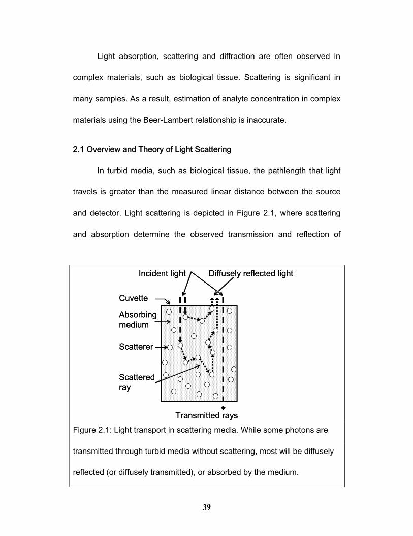
2.1 Overview and Theory of Light Scattering
In turbid media, such as biological tissue, the pathlength that light
travels is greater than the measured linear distance between the source
and detector. Light scattering is depicted in Figure 2.1, where scattering
and absorption determine the observed transmission and reflection of
Incident light
Cuvette
Absorbing
medium
Scatterer
Scattered
ray
Transmitted rays
Diffusely reflected lightIncident light
Cuvette
Absorbing
medium
Scatterer
Scattered
ray
Transmitted rays
Diffusely reflected light
Figure 2.1: Light transport in scattering media. While some photons are
transmitted through turbid media without scattering, most will be diffusely
reflected (or diffusely transmitted), or absorbed by the medium.

40
light. In tissue, light is scattered strongly by small particles,
macromolecules, tissue morphology, and boundaries with mismatched
refractive indices.4 When the light-scattering particle is much smaller than
the wavelength (λ) of light, the scattering is best described by Rayleigh
scattering theory in which the scattering is nearly isotropic and decreases
as a function of λ-4. When the scattering particle is larger than λ, the
scattering is better described by Mie theory where the scattering is
anisotropic and generally forward directed.
Three fundamental optical properties are used to describe turbid
media: the scattering coefficient (μs), asymmetry parameter (g), and
absorption coefficient (μa). Absorption coefficients can be related to
traditional molar absorptivity through
, (2.2)
where ε is the molar absorptivity, c is the concentration of the absorber, L
is the pathlength, and A is the measured absorption. The absorption
coefficient combines the molar absorptivity and concentration terms,
having dimensions of inverse millimetres (mm-1) or centimetres (cm-1).
Absorption coefficients are a measure of absorption events per unit
distance. Corresponding to the absorption coefficient, the scattering
41
coefficient is the average number of scattering events per unit distance.
Optical scattering and absorption coefficients can also be theoretically
derived from the number density (concentration) and the molecular
scattering cross sectional areas which are in turn determined from
molecular volumes and scattering efficiency.5-7 The asymmetry parameter,
g, is used to describe the average scattering direction.8 Also known as the
anisotropy, g is calculated as the average cosine of the scattering angle.
The amount of scattering with respect to the scattering angle can be
plotted as a scattering diagram, also known as a phase function. The
anisotropy varies from -1 to +1, for preferentially forward-directed
scattering g > 0, for anisotropic scattering g = 0 (equal in all directions),
and for preferentially backward-directed scattering g < 1. Scattering
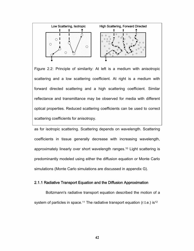
coefficients and anisotropy can be combined into the reduced scattering
coefficient (μs'), based on the principle of similarity.9
ss g 1' (2.3)
Reduced scattering coefficients are used because similar fluence
distributions may be observed between systems with different optical
properties, provided that particular anisotropic conditions are satisfied.
This is illustrated in Figure 2.2. Highly forward directed scattering
decreases the effective scattering coefficient because the average
scattering event does not change the direction of propagation as greatly
42
as for isotropic scattering. Scattering depends on wavelength. Scattering
coefficients in tissue generally decrease with increasing wavelength,
approximately linearly over short wavelength ranges.10 Light scattering is
predominantly modeled using either the diffusion equation or Monte Carlo
simulations (Monte Carlo simulations are discussed in appendix G).
2.1.1 Radiative Transport Equation and the Diffusion Approximation
Boltzmann's radiative transport equation described the motion of a
system of particles in space.11 The radiative transport equation (r.t.e.) is12
Low Scattering, Isotropic High Scattering, Forward DirectedLow Scattering, Isotropic High Scattering, Forward Directed
Figure 2.2: Principle of similarity: At left is a medium with anisotropic
scattering and a low scattering coefficient. At right is a medium with
forward directed scattering and a high scattering coefficient. Similar
reflectance and transmittance may be observed for media with different
optical properties. Reduced scattering coefficients can be used to correct
scattering coefficients for anisotropy.
43
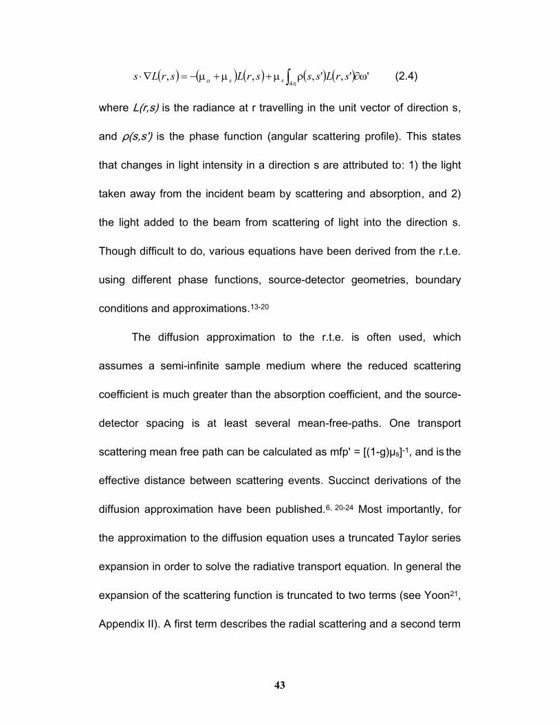
4'',',,, srLsssrLsrLs ssa (2.4)
where L(r,s) is the radiance at r travelling in the unit vector of direction s,
and ρ(s,s') is the phase function (angular scattering profile). This states
that changes in light intensity in a direction s are attributed to: 1) the light
taken away from the incident beam by scattering and absorption, and 2)
the light added to the beam from scattering of light into the direction s.
Though difficult to do, various equations have been derived from the r.t.e.
using different phase functions, source-detector geometries, boundary
conditions and approximations.13-20
The diffusion approximation to the r.t.e. is often used, which
assumes a semi-infinite sample medium where the reduced scattering
coefficient is much greater than the absorption coefficient, and the source-
detector spacing is at least several mean-free-paths. One transport
scattering mean free path can be calculated as mfp' = [(1-g)μs]-1, and is the
effective distance between scattering events. Succinct derivations of the
diffusion approximation have been published.6, 20-24 Most importantly, for
the approximation to the diffusion equation uses a truncated Taylor series
expansion in order to solve the radiative transport equation. In general the
expansion of the scattering function is truncated to two terms (see Yoon21,
Appendix II). A first term describes the radial scattering and a second term
44
describes the forward peaked scattering. Because expansion terms have
been truncated, quantification errors of up to 10% are observed when
comparing theory to measurements.25
The diffusion equation models the transfer of light in both time and
space, though particular solutions have been derived for steady-state
(time-integrated) and time-dependent (spatially-integrated) solutions.
These models of photon transport are most relevant to experimental
observations, because most methods allow the measurement of intensity
with respect to either time or position (but usually not both). In this thesis
both the time-dependent and steady-state approaches were examined.
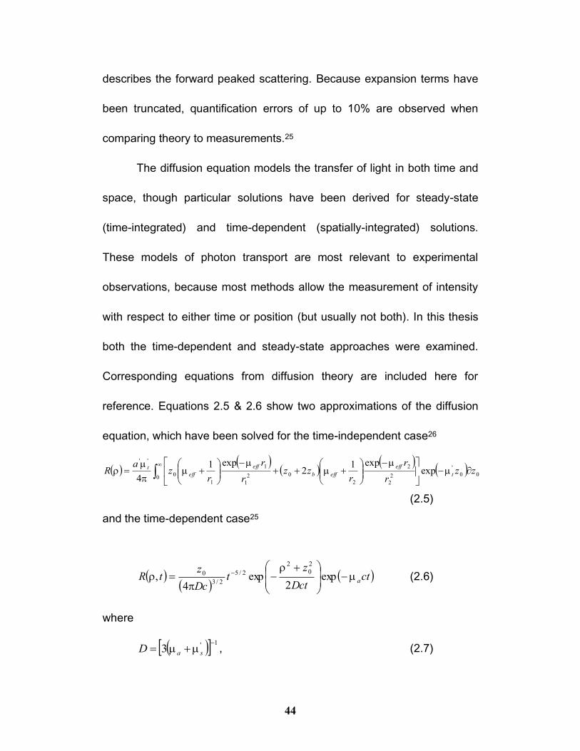
Corresponding equations from diffusion theory are included here for
reference. Equations 2.5 & 2.6 show two approximations of the diffusion
equation, which have been solved for the time-independent case26
000
'
2
2
2
2
02
1
1
1
0
''
expexp1
2exp1
4zz
r
r
rzz
r
r
rz
aR t
eff
effb
eff
eff
t
(2.5)
and the time-dependent case25
ctDct
zt
Dc
ztR a
exp
2exp
4,
2
0
2
2/5
2/3
0 (2.6)
where
1'3
saD , (2.7)
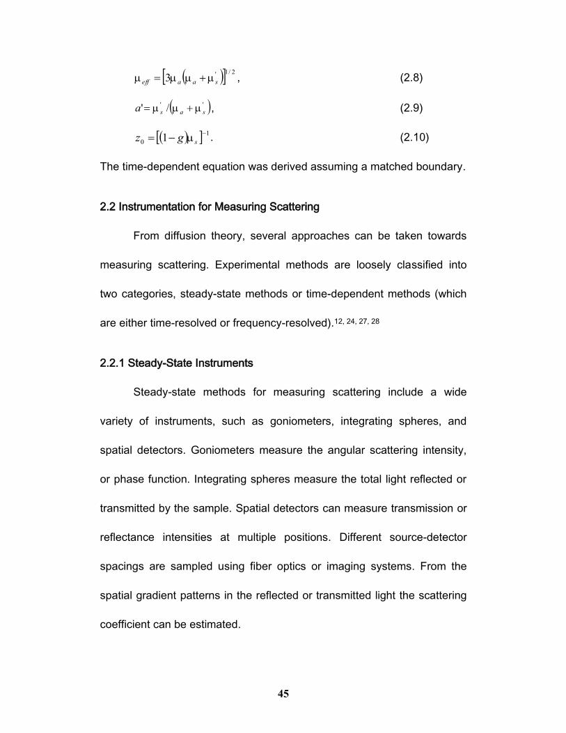
45
2/1'3 saaeff , (2.8)
'' /' sasa , (2.9)
1
0 1
sgz . (2.10)
The time-dependent equation was derived assuming a matched boundary.
2.2 Instrumentation for Measuring Scattering
From diffusion theory, several approaches can be taken towards
measuring scattering. Experimental methods are loosely classified into
two categories, steady-state methods or time-dependent methods (which
are either time-resolved or frequency-resolved).12, 24, 27, 28
2.2.1 Steady-State Instruments
Steady-state methods for measuring scattering include a wide
variety of instruments, such as goniometers, integrating spheres, and
spatial detectors. Goniometers measure the angular scattering intensity,
or phase function. Integrating spheres measure the total light reflected or
transmitted by the sample. Spatial detectors can measure transmission or
reflectance intensities at multiple positions. Different source-detector
spacings are sampled using fiber optics or imaging systems. From the
spatial gradient patterns in the reflected or transmitted light the scattering
coefficient can be estimated.
46
Steady-state imaging systems typically require less complex
electronics than time-resolved instruments. Several methods have been
reported that measure the reflectance of laser beams directed onto the
surface of turbid media. Point detectors (fiber optics) at multiple source-
detector spacings have been used to be sensitive to variations of μa and
μ’s.29 Fiber optic detectors have been reported with radial,30 linear,31, 32
and concentric circle33 arrangements of the detection fiber optics. In
addition to point detection methods, imaging methods have been
demonstrated for estimation of μa and μ’s.34-38 Anisotropy has been
measured by imaging laser beams at a non-normal angle.38 Several
theories and models for quantification of optical properties from steady-
state reflectance have also been investigated.18, 26, 39, 40
47
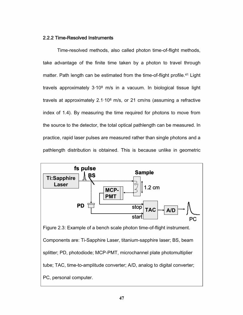
2.2.2 Time-Resolved Instruments
Time-resolved methods, also called photon time-of-flight methods,
take advantage of the finite time taken by a photon to travel through
matter. Path length can be estimated from the time-of-flight profile.41 Light
travels approximately 3·108 m/s in a vacuum. In biological tissue light
travels at approximately 2.1·108 m/s, or 21 cm/ns (assuming a refractive
index of 1.4). By measuring the time required for photons to move from
the source to the detector, the total optical pathlength can be measured. In
practice, rapid laser pulses are measured rather than single photons and a
pathlength distribution is obtained. This is because unlike in geometric
TAC
Ti:Sapphire
Laser
BS
PD
Sample
MCP-
PMT
A/D
1.2 cm
PC
fs pulse
stop
start
TAC
Ti:Sapphire
Laser
BS
PD
Sample
MCP-
PMT
MCP-
PMT
A/D
1.2 cm
PC
fs pulse
stop
start
Figure 2.3: Example of a bench scale photon time-of-flight instrument.
Components are: Ti-Sapphire Laser, titanium-sapphire laser; BS, beam
splitter; PD, photodiode; MCP-PMT, microchannel plate photomultiplier
tube; TAC, time-to-amplitude converter; A/D, analog to digital converter;
PC, personal computer.
48
optics, photons do not follow a single predictable path, but rather follow a
distribution of paths.
Laser pulses are delayed in time and broadened by scattering
because individual photons travel through a distribution of optical paths.
An example of a bench-scale photon time-of-flight instrument is presented
in Figure 2.3. In this example, a Titanium-sapphire laser is used to
generate a brief pulse of light. The pulse is then split by a beam splitter,
with one half starting a clock (TAC), and the other half illuminating the
sample. A single photon microchannel plate photomultiplier tube
(MCP-PMT) detector stops the clock as the first photon exits the sample.
By repeatedly recording the time required for the first photon to escape the
sample, the distribution of residence times is measured. Time-of-flight
profiles have been used to evaluate diffusion theory and Monte Carlo
models.25 Monte Carlo models are described in Appendix G. Time-domain
systems have traditionally been non-portable and costly, preventing the
routine use of these instruments.42
Applications of time-domain systems vary widely, and include such
diverse topics as ultra-fast optics,43 nonlinear optics,44 continuum-pulse
generation,44 frequency resolved systems,45, 46 as well as the spatial,
confocal and coherent interference systems used for tomographic
49
reconstruction.47 Many additional non-chemical applications of time-
domain optical methods are widely used, such as laser range-finding and
mapping (eg. LIDAR).48
Ultra-fast optical laser pulses with very high peak powers generate
nonlinear optical effects in condensed matter.44 Nonlinear optical
interactions of light with matter can lead to spectral broadening due to a
variety of optical phenomena, such as group velocity dispersion and multi-
photon ionization.44 A common use of nonlinear optics is for generation of
white light "continuum" optical pulses (light with continuous wavelength
distributions generated from a high intensity single-wavelength source).44
Traditionally, nonlinear optical broadening required a very high optical
power delivered over a short duration to cause broadening effects in
condensed matter (typically liquids or glasses). Novel optical fiber
structures have recently renewed interest in continuum light generation,
because these structures provide stable nonlinear optical cavities.
Applications of white-light continuum pulses have included time-resolved
spectroscopy in turbid media and broadband optical coherence
tomography for tissue characterization.44, 49-58
Frequency-resolved systems are similar to time-domain systems,
with the difference that frequency-resolved instruments use greater
50
repetition frequencies and the modulation intensities typically span a
smaller contrast range than time-resolved systems. The phase shift and
amplitude response of a turbid medium are measured.45, 46, 59-61 Phase
shift, modulation depth, and the integrated intensity of the optical wave are
then used to estimate optical properties.46, 61-63 Frequency domain
instruments modulate intensity at megahertz frequencies, and so source
and detector requirements have similar temporal requirements as time-of-
flight instruments. Advantages of frequency domain instruments include
simplifications in electronics because the required sinusoidal waveforms
can be easily generated, and because the high duty cycle leads to rapid
signal acquisition.46, 64 Frequency domain measurements have typically
been used to acquire scattering and absorption coefficients at multiple
wavelengths in series, typically at a single location.63 Several studies have
also used frequency-domain measurements at multiple positions to
reconstruct tomographic models of tissue.45, 47, 64
In addition to simple point measurements of temporal or frequency
domain spectra, spatially variant measurements have been used to
reconstruct one, two and three dimensional maps of chemical
composition. One example of optical tomography is the use of multiple
projections of spectra to reconstruct a three dimensional model of the
51
specimen.65 In turbid media, spatial reconstruction is complicated by
scattering. Multiple scattering is difficult to accurately model because real
systems are strongly heterogeneous, requiring complex simulations of
tissue and large numbers of simulated photons to develop accurate
predictions. Methods exist to negate scattering by temporally selecting
photons with known transit times or spatially selecting photons scattered
at a particular location in the sample using confocal optical geometries.66
Time-domain spectroscopy typically takes advantage of ballistic or snake
photons, which pass through a scattering sample without undergoing
scattering or undergoing only a small number of scattering events. These
photons experience minimal deviations in the optical path and so should
follow Beer's law for quantification of analyte. Ballistic photons can be
observed in transmission scattering experiments, and have been reported
in highly scattering tissue phantoms composed of discrete scatterers. In
tissue, rough boundaries with refractive index differences prevent any
strictly ballistic photons from transiting tissue, though photons with short
transit times (snake photons, with forward directed zig-zag paths) may still
be observed.43 Temporal gating has been used to differentiate between
the early-arriving photons and the late-arriving diffusely scattered light.43
Using finite element modeling, multiple time-domain spectra can be
52
combined to reconstruct one-, two-, or three-dimensional models of
scattering media (with several examples concerned with imaging breast
tissue for detection of cancers).67-70
Interference patterns of coherent light can also be used to
discriminate between the light exiting a turbid medium, in order to select
the light escaping from the medium with a particular temporal delay.71-76
By appropriately positioning the reference beam the depth is selected.
Optical Coherence Tomography (OCT) can be used with a single-
wavelength, and also been used with broadband continuum white-light
pulses to map tissue.74 The primary advantage of OCT is the extremely
fine depth resolution. One limitation of OCT is the sampling depth, which
is limited by the exponential decrease of signal intensity with depth and
scattering level. Typical sampling depths in tissue are in the hundreds of
micrometres, while some studies have reported measurements at up to
millimetre depths using infrared light. Confocal Spectroscopy/Microscopy
use optical geometries to block scattered photons from being detected.57
This method has advantages and disadvantages similar to those of OCT,
while using spatial rather than temporal means for isolating non-scattering
photons. Diffuse Optical Tomography (DOT) uses spectra recorded at
various spatial locations or temporal delays to reconstruct the sample,
53
typically without rejecting the signal from diffusely scattered light.65, 77 The
primary advantage is the dramatic increase in optical signal and
simplification of the instrumentation, while the signal processing is more
complex and the spatial resolution is very coarse.
Temporal and frequency domain methods along with their
tomographic variants have been used in a variety of medical applications.
In biological applications the optical power becomes a limiting factor,
because high pulse power with short duration pulses can cause damage
in tissue.78 Pulse power must be carefully selected to avoid tissue damage
while maximizing signal intensity. A multitude of temporal and frequency
domain methods for analysis of biological tissues for medical applications
have been explored.63, 70, 79-83
2.3 Data Processing for Quantitative Spectroscopy in Scattering Media
Many software approaches have been developed for processing
spectral data of scattering samples. Data processing approaches are
varied and roughly correlate to the type of available data. There are three
main types of available data. Quantification of scattering media is based
on data from (1) spectra, (2) optical properties measurements, or (3) a
combination of spectra and optical properties measurements. The first
category of data analysis is when quantification is based only from spectra
54
or images; the second category of data sets is from only from measured
optical coefficients. The third category is when both spectral and
scattering information are used to quantify constituents. A variety of
processing methods have been used for each type of data. This section
reviews recently reported data processing methods for quantification of
components in scattering media. Relevant studies from the past decade
have been included to illustrate the various methods.
2.3.1 Quantification from Measured Spectra
The first category, where only spectral information was used for
component quantification, involves the majority of reported methods. Near
infrared optical quantification via measured reflectance spectra without
additional measured scattering information is a simple approach amenable
toward clinical applications. Routine tissue analysis by diffuse reflectance
NIR spectroscopy is feasible given the availability of high-quality
instruments. Scattering measurements are typically not made because of
the technological difficulties, but the effects of scattering must be
addressed for accurate quantification. This section is further organized
according the techniques used to record the data. Data processing for
measurements using only a few wavelengths are first discussed, followed
by a description of methods using NIR spectra with measurements at
55
hundreds of wavelengths. Full spectra are processed with either explicit or
implicit scatter-correction.
2.3.1.1 Ratiometric Probes and Simple Imaging
The least complex instruments used are probes measuring the
reflectance at several discrete wavelengths. Some examples of this are
probes calculating the reflectance intensity ratio at two wavelengths to
estimate oxygen saturation in tissue.84-86 Instead of measuring several
discrete wavelengths at a single point, colour imaging with red-green-blue
(RGB) cameras can be used to perform similar imaging measurements.
Digital RGB cameras have been used to estimate tissue oxygenation,
again using the intensity ratios of different colours to estimate oxygen
saturation.87, 88 Processing steps for these methods generally consist of a
background subtraction and a scaled ratio of intensities at different
wavelengths.89 Fixed-wavelength devices have the advantage of being
inexpensive and rugged. Potential disadvantages include a lack of
quantification specificity.
56
2.3.1.2 Processing Full Spectra without Measured Scattering
The most common approach to optical quantification in scattering
media uses reflectance spectra measured at a single source-detector
separation. Despite the many quantification studies using only spectral
information, there is no consensus on the optimal processing method.90
Spectral processing methods can be split into two main groups, those
using explicit scatter-correction, and those using implicit scatter-
correction.91
Explicit scatter correction methods include various techniques such
as dividing by a constant value, taking second derivatives, or fitting the
spectra to account for scattering. An example of the first method uses
cuvette-based calibrations with a linear-least squares estimation routine to
estimate component concentration from spectra scaled by a constant
factor of the source-detector separation.92 Spectral derivatives or discrete
differences93 are often calculated as a data pre-processing step because
the wavelength-dependence of scattering is approximately linear (over
short wavelength ranges) and scatter-dependence should be eliminated in
the derivative spectrum.94 Subsequent techniques for processing
derivative data typically use in vitro calibration methods along with inverse
least squares or partial least squares.95-97 These methods use calibrations
57
determined in vitro to estimate properties of the ex vivo or in vivo tissue,
using derivative pre-processing to reduce the effects of scattering. Other
methods used to classifying disease states from derivative pre-processed
spectra include partial-least-squares logistic-regressions and hierarchal
clustering.98, 99 Other extrinsic methods estimate and correct for scattering
directly from the spectrum. Spectral absorption features of water100 and
ratiometric methods based on isosbestic points90 in the recorded spectra
have been used to derive correction measures. However, even for in vitro
tests, isosbestic spectral points are not always consistent, and this is
aggravated by the complicated nature of tissue. Kubelka-Munk theory,
diffusion theory and multiplicative scatter correction are also used to
correct for scatter prior to least squares or partial least squares
estimations.91, 101 Kubelka-Munk theory describes a sample as a
discontinuous set of homogeneous plane-parallel layers. Representative
layer theory was developed more recently and is used to describe a
sample as a continuous set of heteogeneous plane-parallel layers.102
Implicit scatter-correction methods model the spectral data to
compensate for scattering rather than explicitly treating scattering. Implicit
methods include multivariate curve resolution, principal component
analysis,103 and genetic algorithms.104-106
58
2.3.2 Quantification from Optical Properties Measurements
The second category of data processing methods uses time-
domain, spatial-domain, or frequency-domain measurements of samples
to estimate the optical properties and the component concentrations. Full
spectra are not recorded. Because these measurements usually cover
only a few discrete wavelengths, quantification methods are limited to
ratios and parametric equations of the various wavelengths recorded.
Some examples include: spatially-resolved measurements at 674, 849
and 956 nm;107 time-domain measurements at 780 and 830 nm for
estimating hemoglobin oxygen saturation;108 and frequency-domain
measurements at 674, 811, 849, and 956 nm for estimating hemoglobin,
oxyhemoglobin, and water content of cervical tissue.109 This differs from
the spectral-only processing methods because measured absorption
coefficients are used to estimate the component concentrations. This
difference is important because absorption coefficients are scatter-
independent, while measured reflectance as used by spectra-only
methods is scatter-dependant. Discrete-wavelength results can also be
analyzed with finite-element analysis to map spatial properties of the
tissue to subsurface locations. One such example uses a six-wavelength
frequency-domain system to measure absorption and scattering
59
coefficients, which are then used in finite element analysis for volumetric
mapping of lesions in breasts.47
2.3.3 Quantification from Spectra and Optical Properties Measurements
The third group of processing methods use simultaneously
recorded spectra and scattering measurements to quantify tissue
components. Although these methods provide the most complete
information for tissue quantification, widespread use of this approach is
prohibited by the cost and complexity of the instrumentation. While
temporal, spatial, and frequency domain measurements have all been
demonstrated for spectral correction, the majority of the reported
applications have used spatial domain measurements. Correction
methods either correct a single spectrum using measured scattering, or
use multiple measured spectra to deduce the optical properties at each
wavelength.
2.3.3.1 Using One Recorded Spectrum and Diffusion Model Estimation
A single measured diffuse reflectance spectrum can be scatter-
corrected using a separately measured scattering coefficient. Examples
include use of a frequency domain system110 and imaging system111 to
measure the scattering coefficient at a few wavelengths, and subsequently
correct the measured point spectrum. For the frequency domain system,
60
reduced scattering coefficients were estimated using a Levenberg-
Marquardt algorithm to fit the diffusion model to the recorded frequency
domain information. From the scattering coefficients measured at six
wavelengths, the scattering power relationship with wavelength was
determined. The measured point spectrum was then scatter-corrected
using the scattering power relationship and analyzed with a least-squares
algorithm.110 For the spatial domain system, the radial reflectance
intensities at three wavelengths were fit to Monte Carlo models to estimate
the reduced scattering and absorption coefficients. Absorption coefficients
are then used for Beers-law type linear quantifications.
2.3.3.2 Using Many Recorded Spectra
Multi-spectral processing methods are most often used for multiple
spectra recorded at different source-detector spacings, though full-
spectrum time-domain measurements have also been reported.31, 112
Spatial methods estimate the scattering and absorption coefficients by
fitting the intensities recorded at multiple distances to the diffusion
equation.31, 113 Variations on this method can include taking second
differences prior to fitting. Alternately, broadband time-domain
measurements have been demonstrated to directly measure the optical
properties at many wavelengths simultaneously.112 These approaches are

61
elegant and precise. Unfortunately the instrumentation required is complex
and not currently practical for routine clinical measurements.
2.4 Tissue Properties and Spectroscopically Active Bioanalytes
Now that light scattering theory, instrumentation, and processing
methods have been described, we turn to the crux of the issue: what are
the optical properties of tissue and which bioanalytes can be examined?
To begin with, a spectral range must be selected. Section 2.4.1 outlines
the reasons for which the near-infrared spectral region is used for tissue
spectroscopy. Next, some reported optical properties of tissue are listed.
Finally, an overview of optically-active metabolic processes and
bioanalytes of interest are presented.
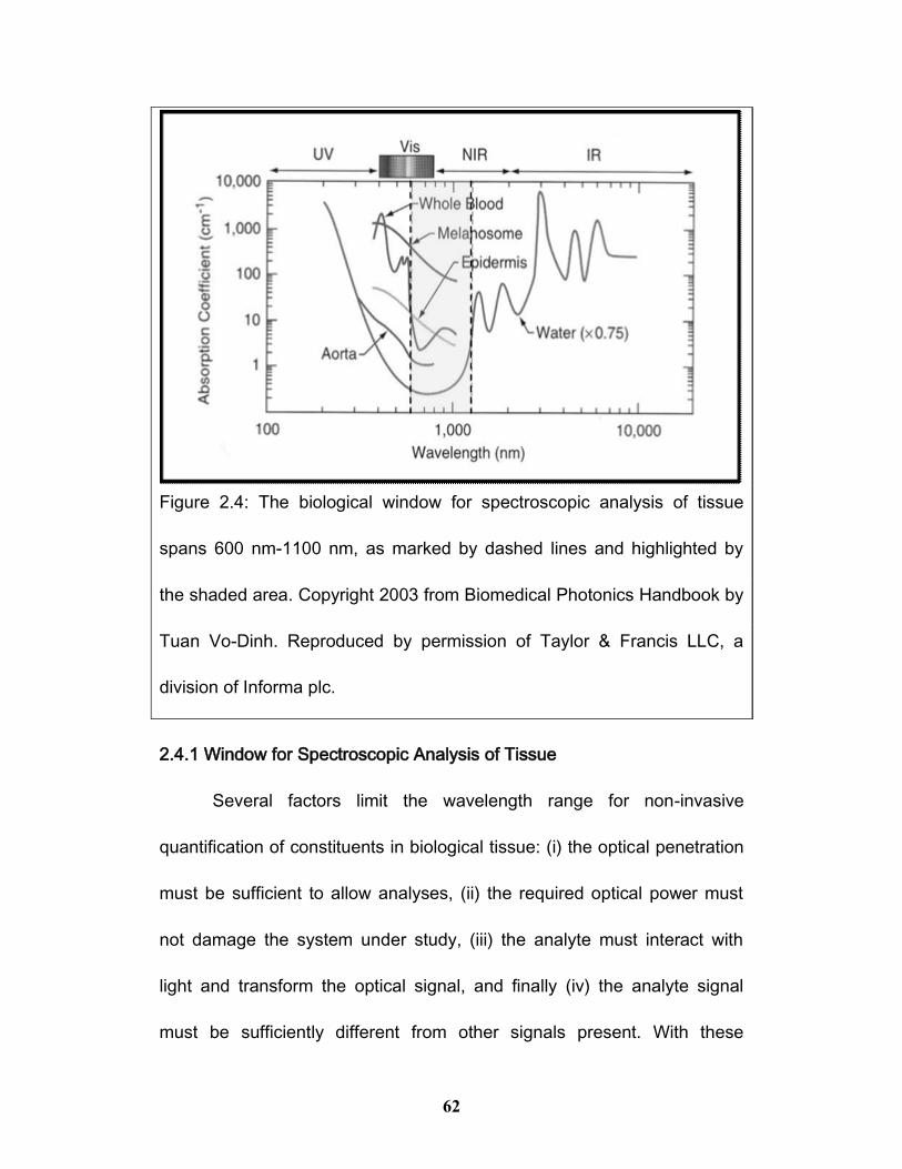
62
2.4.1 Window for Spectroscopic Analysis of Tissue
Several factors limit the wavelength range for non-invasive
quantification of constituents in biological tissue: (i) the optical penetration
must be sufficient to allow analyses, (ii) the required optical power must
not damage the system under study, (iii) the analyte must interact with
light and transform the optical signal, and finally (iv) the analyte signal
must be sufficiently different from other signals present. With these
Figure 2.4: The biological window for spectroscopic analysis of tissue
spans 600 nm-1100 nm, as marked by dashed lines and highlighted by
the shaded area. Copyright 2003 from Biomedical Photonics Handbook by
Tuan Vo-Dinh. Reproduced by permission of Taylor & Francis LLC, a
division of Informa plc.

63
constraints in mind, the best region of the electromagnetic spectrum is in
the visible to near-infrared (600-1100 nm) region. As seen in Figure 2.4,
the spectroscopic window between 600 and 1100 nm is where absorption
of hemoglobin, melanin and water is at a minimum, thus enabling NIR
measurements of bioanalytes such as hemoglobin, lactate, glucose, or
bilirubin. Toward the near-infrared region of the window, light may
penetrate several centimetres into tissue, and several bioanalytes have
absorption features. Moreover, optical sources and detectors are well-
developed for this region. However, absorption features are broad and
non-specific. Use of light in the near-infrared region allows non-invasive
biomedical measures with lower cost and complexity than other spectral
regions.114 As a result, the near-infrared spectral region is a practical
spectral region for the development of simplified instrumentation.
However, because of the broad absorption features in near-infrared
spectra and interference by light scattering, the potential of in vivo near-
infrared spectroscopy for clinical purposes has not yet been fulfilled.115
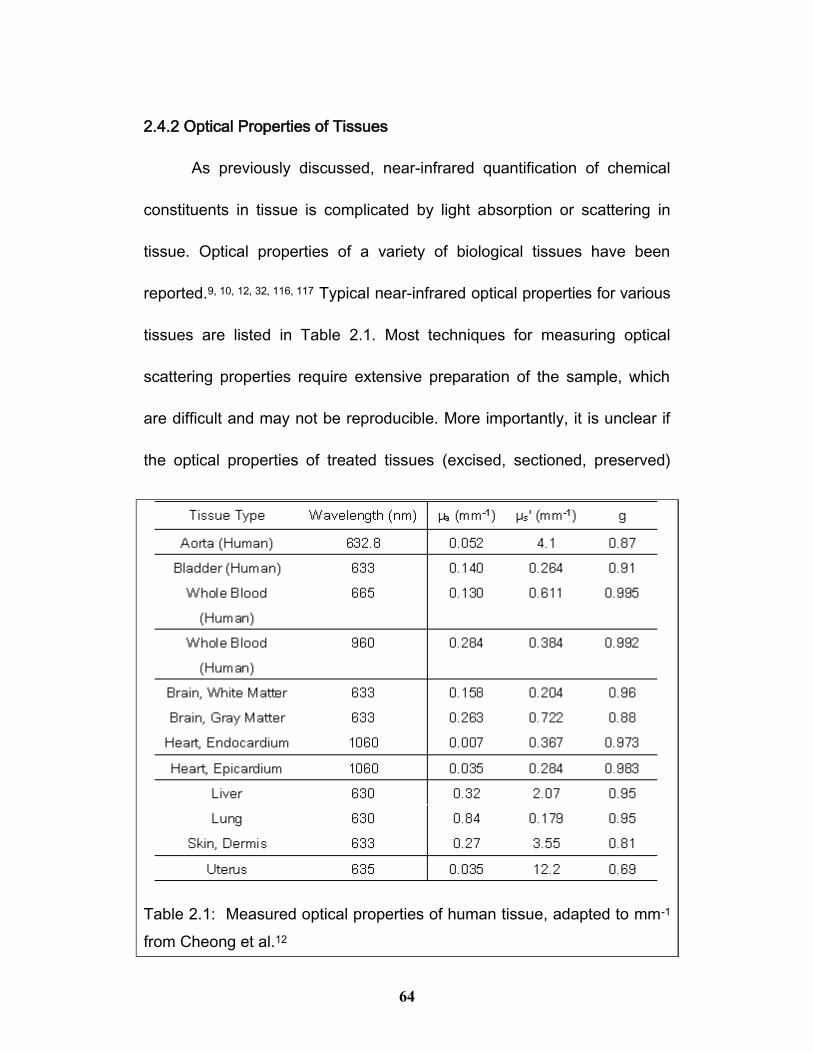
64
2.4.2 Optical Properties of Tissues
As previously discussed, near-infrared quantification of chemical
constituents in tissue is complicated by light absorption or scattering in
tissue. Optical properties of a variety of biological tissues have been
reported.9, 10, 12, 32, 116, 117 Typical near-infrared optical properties for various
tissues are listed in Table 2.1. Most techniques for measuring optical
scattering properties require extensive preparation of the sample, which
are difficult and may not be reproducible. More importantly, it is unclear if
the optical properties of treated tissues (excised, sectioned, preserved)
Table 2.1: Measured optical properties of human tissue, adapted to mm-1
from Cheong et al.12
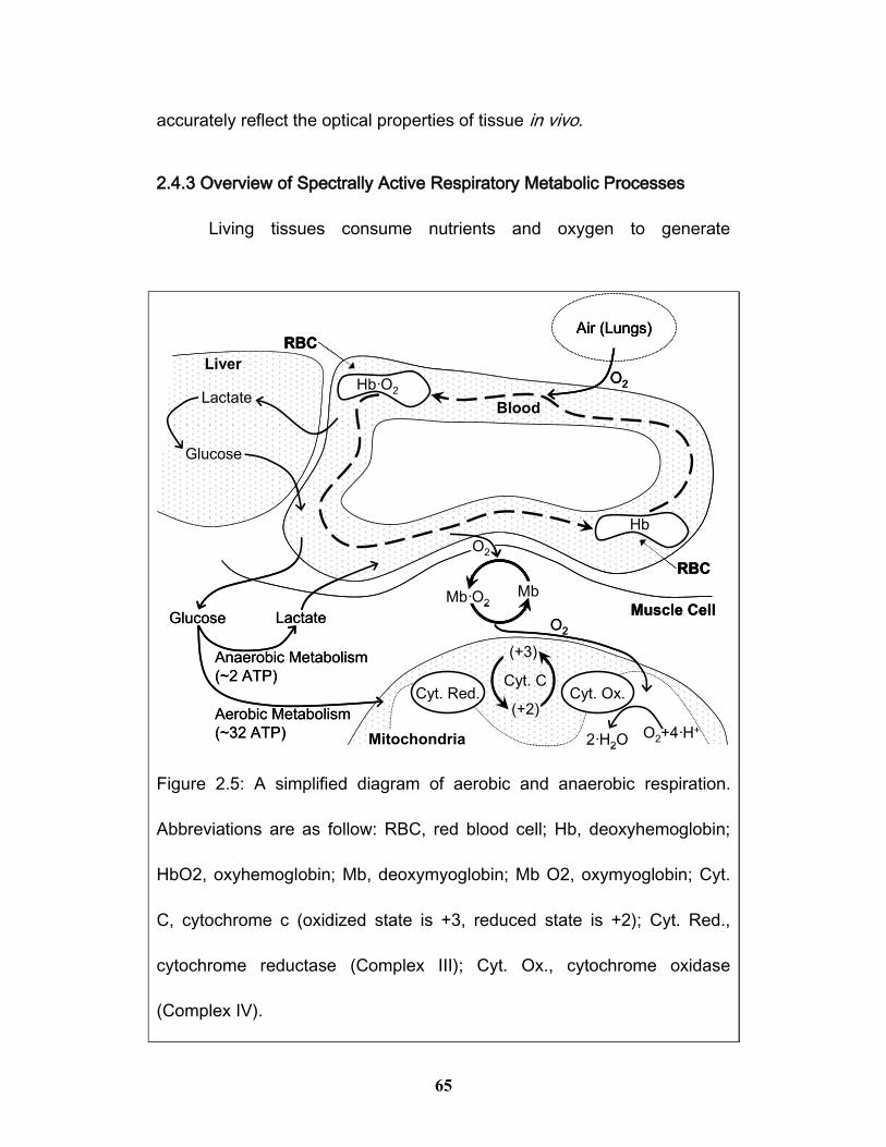
65
accurately reflect the optical properties of tissue in vivo.
2.4.3 Overview of Spectrally Active Respiratory Metabolic Processes
Living tissues consume nutrients and oxygen to generate
Circulatory System
Blood
RBC
RBC
Hb·O2
Hb
Muscle Cell
Air (Lungs)
O2
O2
Mb·O2Mb
Liver
Lactate
Glucose
Glucose Lactate
Anaerobic Metabolism
(~2 ATP)
Mitochondria
(+2)
Cyt. C
(+3)
Cyt. Red. Cyt. Ox.
Aerobic Metabolism
(~32 ATP)
O2
O2+4·H+2·H2O
Circulatory System
Blood
RBC
RBC
Hb·O2
Hb
Blood
RBC
RBC
Hb·O2
Hb
Muscle Cell
Air (Lungs)
O2
Air (Lungs)
O2
O2
Mb·O2MbMb·O2Mb
Liver
Lactate
Glucose
Glucose Lactate
Anaerobic Metabolism
(~2 ATP)
Mitochondria
(+2)
Cyt. C
(+3)
Cyt. Red. Cyt. Ox.
Aerobic Metabolism
(~32 ATP)
O2
O2+4·H+2·H2O
Figure 2.5: A simplified diagram of aerobic and anaerobic respiration.
Abbreviations are as follow: RBC, red blood cell; Hb, deoxyhemoglobin;
HbO2, oxyhemoglobin; Mb, deoxymyoglobin; Mb O2, oxymyoglobin; Cyt.
C, cytochrome c (oxidized state is +3, reduced state is +2); Cyt. Red.,
cytochrome reductase (Complex III); Cyt. Ox., cytochrome oxidase
(Complex IV).

66
biochemical gradients across cellular membranes. Concentration
gradients drive the flow of energy required for many respiratory processes
in living organisms. A broad overview of the metabolic pathways for
spectrally active oxygen binding proteins, glucose and lactate are shown
in Figure 2.5. Proper function of metabolic processes can be examined by
measuring oxygen partial pressure or nutrient concentrations.
Interruptions to the respiratory system are a prominent cause of metabolic
failure and subsequently cellular death. Ultimately, this is summarized by
the saying: "if you don't breathe, you die."
Some bioanalytes have spectral features and can serve as
indicators of oxygen partial pressure. These bioanalytes can be used to
determine the state of oxygen consumption, oxygen delivery, and also
metabolic activity. Spectroscopically active indicators of oxygen partial
pressure include: hemoglobin in blood, myoglobin in muscle tissue, and
cytochromes in mitochondria. These proteins reversibly bind oxygen in
proportion to the local oxygen partial pressure. As a result, the ratio of
each oxygenated species to the total concentration of that species may
function as a localized indicator of oxygen partial pressure. Significant
oxygen pressure gradients exist in tissue because oxygen diffuses
through blood, tissue and cellular membranes at different rates. The

67
integrated oxygen saturation of hemoglobin, myoglobin or cytochromes is
proportional to the rate of oxygen consumption.
Glucose and lactate concentrations can also be optically measured
to gauge the efficiency of metabolic energy flow in tissue. As seen in
Figure 2.5, transport of oxygen and production of simple carbohydrates
are key functions in aerobic and anaerobic metabolism.118 Under
anaerobic conditions, lactate is produced and builds in tissues during
times of high energy demand. Glucose is converted to energy in the form
of adenosine 5’-triphosphate (ATP) through the processes of glycolysis
and the citric acid cycle. Oxygen supplied to cells is consumed in the
conversion of glucose to energy.
Determination of these metabolic indicators in vivo is instrumental
in further understanding metabolic processes in both healthy and diseased
tissue. Respiratory pathways have been studied extensively by NIR
spectroscopy because spectra change rapidly in response to its local
chemical environment. In particular, NIR spectra of myoglobin and
hemoglobin are strongly responsive to oxygenation state. Rapid
measurement of myoglobin or hemoglobin oxygenation has important
clinical applications of maintaining proper oxygen levels during surgery
and monitoring the patient for respiratory failure.
68
Hemoglobin and myoglobin are metalloproteins found in red blood
cells and muscle tissue, respectively. The absolute concentration and
relative oxygenation of these proteins can be used to measure the relative
‘health’ of tissues during surgery or as a response to medical treatment.
Both proteins function as an oxygen transport and storage network which
enhances oxygen transport into tissue in comparison to simple
diffusion.119
Hemoglobin and myoglobin have iron-containing heme groups,
which reversibly bind to oxygen. Heme strongly binds oxygen in an
'end-on bent' geometry, and a distinctly modified NIR spectrum is
observed as compared to oxygen-free heme. As seen in Figure 2.6, the
NIR spectrum of deoxyhemoglobin is similar to the NIR spectrum of
deoxymyoglobin.120 The myoglobin spectrum is red-shifted by
approximately 3 nm with respect to the spectrum of hemoglobin. In the
region from 450 to 960 nm, principal features of oxygen-free spectra are
maxima at approximately 555, 755 and 910 nm. The corresponding
primary feature of the oxy spectra is an incompletely resolved pair of
maxima at 545 and 575 nm.
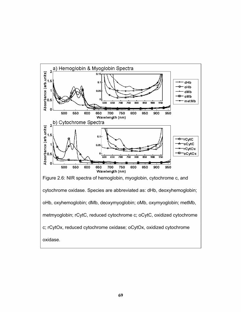
69
Figure 2.6: NIR spectra of hemoglobin, myoglobin, cytochrome c, and
cytochrome oxidase. Species are abbreviated as: dHb, deoxyhemoglobin;
oHb, oxyhemoglobin; dMb, deoxymyoglobin; oMb, oxymyoglobin; metMb,
metmyoglobin; rCytC, reduced cytochrome c; oCytC, oxidized cytochrome
c; rCytOx, reduced cytochrome oxidase; oCytOx, oxidized cytochrome
oxidase.

70
Oxygen partial pressure in tissue can be measured using NIR
spectroscopy because the NIR spectra of hemoglobin and myoglobin are
modified with oxygenation, and a ratio of oxygenated protein to total
protein can be measured. Spectra of cytochrome oxidase and cytochrome
c are also shown in Figure 2.6. Cytochrome c is a protein with a heme
group at the center, which is bound to a methionine on one face and
histidine on the other, which transports electrons in respiration. Spectral
features of the cytochromes overlap with spectral features of hemoglobin
and myoglobin, and these may interfere with hemoglobin and myoglobin
oxygen saturation measurements. Other hemoglobin and myoglobin forms
are also present in the body, such as carboxyhemoglobin and
metmyoglobin, and may further complicate analysis of NIR spectra.121, 122
In the ideal case, all spectroscopically active components would be taken
into account to better compensate for these optical interferences. In
practice, often only the concentrations of the most spectroscopically active
species are estimated.
2.4.4 Hemoglobin Oxygen Saturation Measurement
Spectroscopic determination of hemoglobin oxygen saturation is an
active area of research.121, 123-126 Photoplethysmography is the use of
optical absorption to measure the cardiovascular pulse wave and
71
hemoglobin oxygen saturation. In simple implementations, an intensity
ratio of the oxyhemoglobin signal is compared to signal at an isosbestic
point combining hemoglobin and oxyhemoglobin at a second wavelength.
Oxygen saturation in the blood is typically measured from signal ratios, as
described in section 2.3.1.1 above.
Improved reliability and imaging modalities are active research
areas in photoplethysmography.87, 127 Pulse-oximetry, another application
of optical absorption, was invented early in the twentieth century, and is
used to measure blood oxygen saturation.128, 129 Pulse-oximetry is the
most widely-used commercial application of non-invasive NIR biomedical
spectroscopy. Pulse-oximetry measures differences in spectra at the
maximum and the minimum pulsatile volumes. The pulsatile variation is
observed in tissue by rapidly measuring the intensities of two wavelengths
(usually 660 and 940 nm) corresponding to deoxy- and oxy-hemoglobin.
As the heart beats, blood pulses through tissue capillaries and can be
seen as a waveform in the intensities. The DC signal from the tissue
background and non-pulsatile blood components is subtracted by taking
the difference between the maximum and minimum values in the AC
waveform. This process allows for experimental differentiation between
the pulsatile component of blood and the non-pulsatile components of

72
blood and other tissues.130 The remaining AC signal is attributed to
hemoglobin absorption, and hemoglobin oxygen saturation is calculated
as the ratio of the two wavelengths. A clear presentation of pulse oximetry
is given in "Design of Pulse Oximeters."131 Oxygen saturation is calculated
as the fraction of a species bound to oxygen, and so hemoglobin oxygen
saturation is calculated as
100
2
2,2
HbOHb
OHbS HbO (2.7)
where [Hb] is the concentration of hemoglobin, [Hb·O2] is the
concentration of oxyhemoglobin, and S is the unitless percent oxygen
saturation of hemoglobin. Myoglobin oxygen saturation can be calculated
by substituting myoglobin for hemoglobin in the Equation 2.7. Myoglobin
concentration does not vary with the heartbeat because it is normally
located entirely in muscle tissue. While both pulse-oximetry and
photoplethysmography estimate hemoglobin oxygen saturation, neither
method measures absolute hemoglobin concentrations.132 Absolute
hemoglobin concentration is about 50 μM in aerobic skeletal muscle, and
because hemoglobin contains four heme subunits, the heme
concentration should be about 200 μM.120 Capillary density in cardiac
muscle is higher than in skeletal muscle, and the heme concentration
should also be higher. 120 Myoglobin concentration in skeletal muscle
73
should be about 250 μM.120 In muscle, hemoglobin heme and myoglobin
heme should be present in nearly equal proportions. Saturation is typically
measured as a difference in saturation compared to an arbitrary starting
point. Single-point measures of hemoglobin oxygen saturation can be
improved by taking into account light scattering, the presence of
myoglobin and cytochromes, and spatial localization of the signal
sources.127 The accuracy of hemoglobin oxygen saturation measurements
can also change with absolute concentration.63 A better understanding of
tissue dynamics can be realized by mapping the saturation values to
either the surface of the skin or to the subsurface tissue volume.87, 133
Estimations can be can be further improved by measuring entire spectral
profiles and using more complex data analysis techniques instead of
measuring saturation from only a few discrete wavelengths.
2.4.5 Myoglobin Oxygen Saturation Measurement
NIR spectroscopy has potential to assess oxygenation of myoglobin
in cardiac tissue during surgery, prior to tissue necrosis. However,
isolation of spectral features in tissue that can be solely attributed to
myoglobin is difficult because of both light scattering and because spectral
properties of myoglobin and hemoglobin share similar spectral absorption
features.
74
Nuclear magnetic resonance spectroscopy (NMR) can be used to
measure the 1H deoxymyoglobin signal independently from the
hemoglobin signal, and several groups have used magnetic resonance
imaging (MRI) to study myoglobin oxygen saturation in working muscle.134
There are many situations where MRI instrumentation is impractical
because of the strong ambient magnetic field and constrained working
area, for example inside of a surgical suite.
Most optical studies of myoglobin oxygen saturation in biological
tissue have experimentally removed hemoglobin prior to measuring the
spectra by perfusing the tissue with hemoglobin-free buffer solutions.
Elimination of hemoglobin is not feasible when examining tissue in vivo.
Instead, data reduction techniques can be applied to NIR spectra and
estimation of myoglobin oxygen saturation can be obtained.97, 135, 136 To
apply these partial least squares data processing techniques the optical
properties of the in vitro calibration model must sufficiently represent the
optical properties of the working system. Classical least squares (CLS)
can also be used to estimate myoglobin oxygen saturation. Classical least
squares regressions require the measurement of the 0% and 100%
saturation endpoints.

75
2.4.6 Carbohydrate and Other Spectral Features
Glucose and lactate are spectroscopically active bioanalytes with
distinct NIR spectral features. Figure 2.7 shows the NIR spectra of lactate
and glucose. Additional components of tissue that can be measured using
NIR spectroscopy are melanin, water, adipose tissue, and calcifications.
NIR measurements of lactate, melanin, water, and adipose have been
shown in tissue, reflecting the applicability of NIR to help diagnose many
medical disorders.24, 86, 95, 137-143 The near infrared spectrum of water is
sensitive to temperature because temperature affects hydrogen bonding
of water. Tissue temperature can be estimated from water spectra.104, 144
Of the many spectroscopically active metabolic components, in vivo
glucose measurements are the most commonly studied. More recently,
near infrared measurements of lactate have been increasingly studied.
Non-invasive glucose measurement is of significant medical
interest because of the prevalence of diabetes. Current blood glucose
measurements require patients to draw blood for analysis, and a
non-invasive optical method would be preferable. Despite great interest in
non-invasive glucose diagnostics, optical glucometers are not yet readily
commercially available. In the near-infrared glucose has a broad spectral
absorption band from 1550 to 1850 nm as shown in Figure 2.7b, which

76
overlaps with NIR spectral features of water and tissue. Spectral overlap
and low tissue glucose concentration presents significant challenges in
tissue glucose quantification. Progress in near infrared glucose
diagnostics has been summarized in many review articles.91, 145-149 Rapid,
non-invasive optical measurement of glucose has potential as a home-
based detection system that can be used by diabetes patients to maintain
proper insulin levels.91, 150
Near infrared tissue lactate measurements can be used to estimate
anaerobic exercise thresholds, and may also facilitate monitoring of tissue
perfusion in surgery and trauma. Lactate has three near infrared
absorption bands at 1675, 1690, and 1730 nm, as shown in Figure 2.7a.
These spectral features were used by Lafrance to measure lactate
in vivo.95 To the best of our knowledge, this is currently the only study
reporting in vivo measurement of lactate using the near infrared. Several
other studies have reported the measurement of lactate in whole blood,
plasma, and other media.137, 138, 151, 152 In chapter 5, processing models for
non-invasive quantification of lactate in tissue are further discussed.
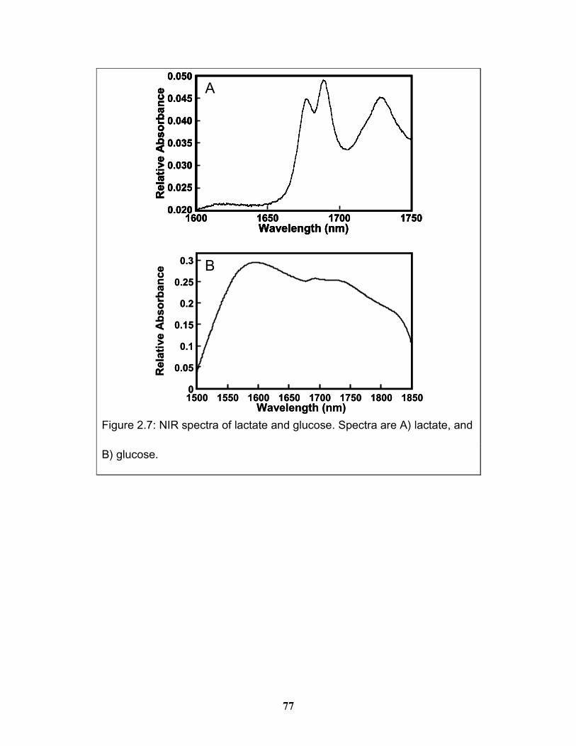
77
1500 1550 1600 1650 1700 1750 1800 18500
0.05
0.1
0.15
0.2
0.25
0.3
Wavelength (nm)
Rela
tive A
bso
rban
ce
1600 1650 1700 1750
0.035
0.045
0.050
Rela
tive A
bso
rban
ce
0.020
0.025
0.030
0.040
Wavelength (nm)1600 1650 1700 1750
0.035
0.045
0.050
Rela
tive A
bso
rban
ce
0.020
0.025
0.030
0.040
Wavelength (nm)
B
A
Figure 2.7: NIR spectra of lactate and glucose. Spectra are A) lactate, and
B) glucose.
78
Chapter 3. A Portable Multi-Wavelength Near-
Infrared Photon Time-of-Flight Instrument for
Measuring Light Scattering
To correct for light scattering, scattering coefficients can be
measured and mathematically corrected for. One method of measuring
scattering involves measurement of the time required for a pulse of
photons to propagate through a medium. Such photon time-of-flight
systems have been used to measure scattering coefficients of turbid
media. In this chapter, a simplified photon time-of-flight system is
described for measuring reduced scattering coefficients and improving
chemical quantification in turbid media. Measured scattering coefficients
are used to correct near-infrared spectra for quantification. Contemporary
photon time-of-flight instruments are impractical for most clinical
biomedical problems. The simplified instrument presented here is both
cost-effective and practical for use in many fields. This system was
developed for measuring scattering coefficients of tissue, with the initial
intention of using this pulsed-light system to augment co-measured
visible-near infrared spectra of heart tissue.
79
In the biomedical field, the time-of-flight instrument may be useful
for improving measurements of tissues and molecular species such as
hemoglobin, myoglobin, cytochrome, glucose, and lactic acid
concentrations, water and lipid content, as well as tissue temperature.28, 47,
91, 137, 144, 153, 154 This photon time-of-flight instrument is practical for
correction of reflectance spectra in simple clinical biomedical applications.
The time required for measurements, as well as the size and financial cost
of the required instrumentation determine the practicality of biomedical
measurements. Point-sampling instruments can be built with a minimal
cost and complexity, leading to practical applications. Hemoglobin oxygen
saturation and temperature are examples of biomedical properties
currently measured by doctors using point-sampling optical
measurements. This simple method for measuring light scattering can be
used to enhance spectral information and improve practical
biodiagnostics.
Liquid samples with known optical properties were used to calibrate
and test the time-of-flight instrument. The optical properties of biological
tissues vary with time and can not be easily controlled. Rather than using
biological samples for calibration and testing, dilute Intralipid/dye solutions
were used as tissue simulating phantoms. Additional information about
80
tissue simulating phantoms is provided in Appendix F. Intralipid is a
commercially prepared oil-in-water emulsion normally used for intravenous
feeding. Intralipid is a practical scattering agent for phantom tissue
because it is readily available, has a comparable refractive index to tissue
membranes, and can easily be formed into various optical geometries.
3.1 Manuscript
A Portable Multi-Wavelength Near-Infrared Photon Time-of-Flight
Instrument for Measuring Light Scattering
Authors:
Francis W.L. Esmonde-White and David H. Burns
3.2 Abstract
Measured light scattering properties can be used to improve
quantitative spectroscopic analyses of turbid samples.155 Instruments
currently used to measure scattering coefficients are not optimized for
portability. A hand-held, dual-wavelength instrument was developed and
validated for rapid measurement of reduced scattering coefficients in
tandem with near-infrared spectra. Intralipid/dye tissue simulating
phantoms were used to model clinically relevant optical properties.
Time-dependent intensity profiles of diffusely reflected near-infrared
pulsed laser light were collected from phantoms and processed to

81
estimate scattering coefficients. In turbid solutions, optical scattering was
measured at 850 and 905 nm with coefficients of variation of 14.1% and
11.6% over a clinically-relevant reduced scattering coefficient range from
1 to 6 mm-1. This dual-wavelength scattering measurement provides a
practical method for measuring optical scattering. A 35% improvement in
quantification of an absorbing dye is shown by incorporating the measured
reduced scattering coefficients when processing NIR spectra. We discuss
the new instrument, methods for estimating the scattering coefficient from
the measured temporal profiles, and finally how the reduced scattering
coefficient is used to correct NIR measurements. Correction of near-
infrared spectra using optical scattering measurements offers one
direction for improving practical non-invasive biomedical quantification
techniques.
3.3 Keywords
diffuse reflectance, near-infrared spectroscopy, photon
time-of-flight, pulsed laser diode, scattering coefficient, optical transport
coefficient, turbid media, biomedical spectroscopy
3.4 Introduction
Near-infrared (NIR) spectroscopy is an established analytical tool in
the analysis of goods, such as foods and pharmaceuticals.155-157 Diffuse

82
reflectance NIR spectroscopy, in the window from 600 to 1100 nm, has
also gained attention as a biomedical diagnostic tool.28 NIR spectroscopy
is attractive because measurements are rapid, non-invasive, low-cost, and
the diffuse reflectance sampling geometry is simple to implement. In the
biomedical field, NIR spectroscopy has been used to investigate tissues
and molecular species such as hemoglobin, myoglobin, cytochrome,
glucose, and lactic acid concentrations, water and lipid content, as well as
tissue temperature.28, 47, 91, 137, 144, 153, 154 In some diseases, such as
osteoarthritis, treatments are available but there is a lack of simple, rapid
and accurate diagnostic tests, in particular for early disease stages. Subtle
chemical changes in the cellular matrix or blood provide indications of
disease. NIR spectra are sensitive to the local chemical environment,
which is modified by disease. Changes in NIR spectra have been shown
to accurately diagnose disease in a variety of tissues and biofluids.
Identification of cancer in breast and pancreatic tissue using NIR has been
demonstrated. Additional applications of NIR spectroscopy include
identification of skin-alterations in diabetes and artherosclerotic plaques,
examination of dental caries, and detection of burns.69, 98, 99, 158-161
Despite promising studies using NIR spectroscopy to examine
normal and diseased tissue, widespread use for in vivo measurements
83
has been limited by response variability due to light scattering. In systems
with scattering, such as tissue, there is a nonlinear relationship of
absorbance to concentration, absorption coefficient, and pathlength. Light
scattering adds significant complexity to NIR measurements. Optical
scattering properties of tissue are sensitive to variations of the chemical
and structural composition of the tissue.162 Complex structures and
dynamics of tissue lead to variations in the optical pathlength even
between replicate measurements in a single sampling zone. These
pathlength variations alter the reflectance efficiency and result in a wide
distribution of observed absorbances.27 Moreover, light scattering and
attenuation is nonlinearly dependent on wavelength. Accurate quantitative
measurements are not possible without correction for variations of
scattering. Thus, light scattering presents a significant hurdle to robust
clinical NIR measurements.
Variation of optical pathlength due to scattering presents a two-fold
problem in diffuse reflectance NIR spectroscopy. First, the collection
efficiency changes independently of absorption and adds a significant
background that is not corrected by traditional reference measurements.
Attenuation has different background offsets at different scattering levels.
Second, the mean path of light through an absorbing medium will be

84
changed nonlinearly with scattering, leading to nonlinear attenuation
changes.
Approaches have been developed to correct for scattering in
attenuation spectra.155, 163 Scatter correction methods include data-
processing (or software techniques) and experimental (or hardware
techniques). Data processing methods include using internal standards
(e.g. solvent absorption bands), derivative spectroscopy, and multiplicative
signal correction. Experimental correction methods measure the reduced
scattering coefficient and correct the attenuation spectra for pathlength
variations. Scattering varies with wavelength, approximately linearly over
short wavelength ranges. Dual-wavelength scattering measurements can
be used to improve spectral corrections through a linear interpolation of
the scattering background.
Measurements of the reduced scattering coefficient are used to
improve estimation of chemical concentrations from NIR spectroscopic
measurements. Mean pathlength in the sample is related to the reduced
scattering coefficient. Time-resolved instrumentation allows precise
measurement of scattering.41 Typical time-resolved instruments include a
picosecond laser source, single photon detectors, and high-speed
electronics.112, 164 Though instrumentation capable of precisely measuring
85
scattering coefficients is common in academic research institutions,
practical instruments are necessary to correct for scattering in clinical NIR
spectroscopic applications. We report development of a portable
instrument for measuring scattering and absorption coefficients at two
wavelengths.
3.5 Method
An instrument was developed to measure reduced scattering
coefficients and reflectance spectra. Measuring scattering coefficients in
addition to reflectance spectra enables correction for the scattering
pathlength. A photon time-of-flight system was developed to measure
reduced scattering coefficients. A commercial diode array spectrometer
was used to simultaneously measure visible-NIR reflectance spectra. A
fiber optic probe was developed for measuring scattering coefficients and
spectra over a small tissue region. Finally, software for the processing of
the recorded time-of-flight and spectral data was developed.
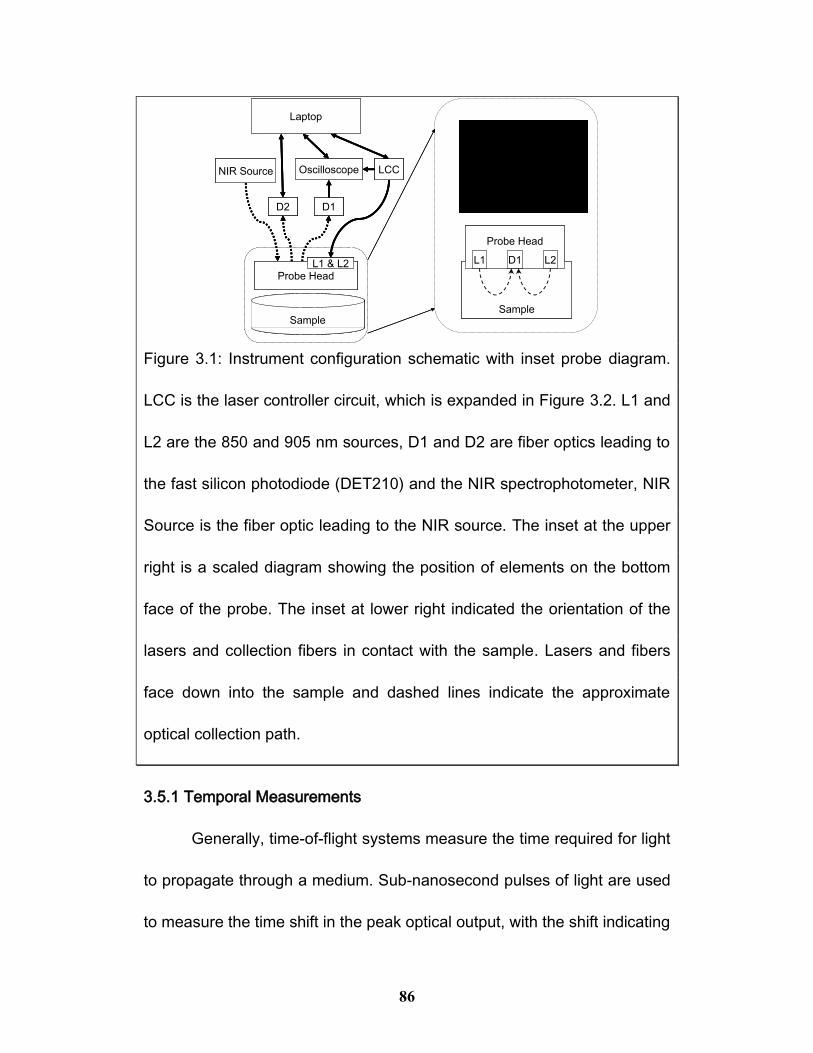
86
3.5.1 Temporal Measurements
Generally, time-of-flight systems measure the time required for light
to propagate through a medium. Sub-nanosecond pulses of light are used
to measure the time shift in the peak optical output, with the shift indicating
Sample
Probe Head
L1 L2D1
Probe HeadL1 & L2
Laptop
D1
Oscilloscope LCC
D2
NIR Source
SampleSample
Probe Head
L1 L2D1
Probe HeadL1 & L2
Laptop
D1
Oscilloscope LCC
D2
NIR Source
Sample
Probe HeadL1 & L2
Laptop
D1
Oscilloscope LCC
D2
NIR Source
Sample
Figure 3.1: Instrument configuration schematic with inset probe diagram.
LCC is the laser controller circuit, which is expanded in Figure 3.2. L1 and
L2 are the 850 and 905 nm sources, D1 and D2 are fiber optics leading to
the fast silicon photodiode (DET210) and the NIR spectrophotometer, NIR
Source is the fiber optic leading to the NIR source. The inset at the upper
right is a scaled diagram showing the position of elements on the bottom
face of the probe. The inset at lower right indicated the orientation of the
lasers and collection fibers in contact with the sample. Lasers and fibers
face down into the sample and dashed lines indicate the approximate
optical collection path.
87
the distance light has traveled in the medium. With longer pulses, changes
in the optical waveform shape are used to estimate the reduced scattering
coefficient. Rising and falling edges change shape with scattering, even
when the total time shift is small relative to the duration of the pulse.
In the current system two laser diodes, SPL-LL85 and SPL-LL90
(OSRAM Opto Semiconductors GmbH, Regensburg, Germany), are used
to generate nanosecond optical pulses. An oscilloscope (SDS-200,
SoftDSP, Seoul, Korea) is then used to record the signal of reflected light
as detected with a high speed photodiode. The optical system is shown in
Figure 3.1, with details of the optical probe shown inset in the upper right
corner. A collection fiber optic spaced 2 mm from the laser diode was
used to channel diffusely reflected light to the photodiode. An electronic
control system was developed to control the pulse repetition frequency,
pulse duration and to choose the output laser wavelength. The electronic
control system was integrated onto a printed circuit board measuring
8.3 x 8.3 cm.
Figure 3.2 shows a diagrammatic representation of the control
circuit board. This system allowed computer control of a microcontroller
through the universal serial bus. The microcontroller produced a trigger
signal used to activate a pulse generator (DS1040, Dallas Semiconductor
88
Corp., Dallas, Texas, USA) and to synchronize the oscilloscope
recordings. Pulse repetition frequency was dynamically set in the
microcontroller and pulse repetition frequency was configured as 1 kHz.
Pulse duration was set to 20 ns using the pulse generator. A high-speed
amplifier (EL7104, Intersil, Milpitas, California, USA) was used to amplify
the trigger pulse for switching the laser diodes on and off. Laser frequency
was selected using transistor switches (2N7002, Digikey) to enable power
to only one laser diode at a time.
Characterizing the laser system required measurement of the laser
output intensity and pulse shapes. Average power of the 850 nm laser
was 182.0 μW +/- 2%. Average power of the 905 nm laser was
187.1 μW +/- 2%. To verify the temporal profile of the laser output,
reflectance from a roughened metal surface was recorded as shown in
Figure 3.4. Reflectance from the metal surface measures the temporal
response profile of the system without diffusion. Optical pulse widths were
measured as 24 ns FWHM for both lasers. Temporal response is limited
primarily by the oscilloscope, having an analog bandwidth of 200 MHz, a
real-time sampling rate of 100 million samples per second and an
equivalent sampling rate of 5 billion samples per second through over-
sampling with a 200 ps time-to-digital converter.
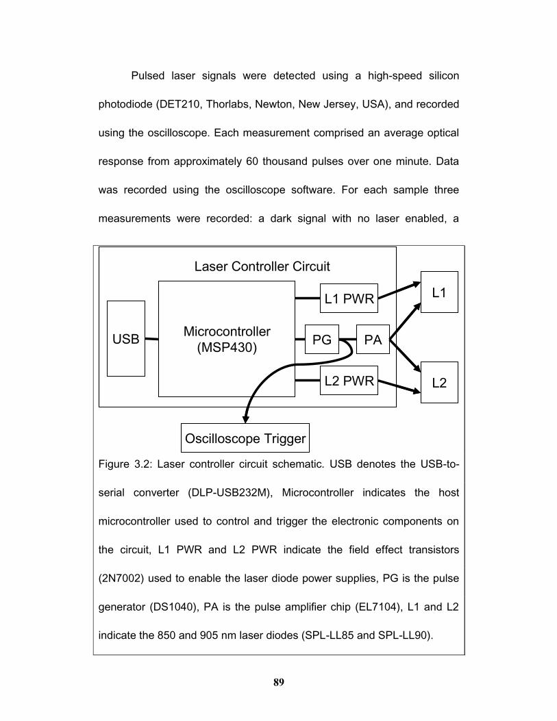
89
Pulsed laser signals were detected using a high-speed silicon
photodiode (DET210, Thorlabs, Newton, New Jersey, USA), and recorded
using the oscilloscope. Each measurement comprised an average optical
response from approximately 60 thousand pulses over one minute. Data
was recorded using the oscilloscope software. For each sample three
measurements were recorded: a dark signal with no laser enabled, a
Laser Controller Circuit
USB
L1 PWR L1 PWR
L2 PWR L2 PWR
L1
L2
PA PAPGMicrocontroller
(MSP430)
Oscilloscope Trigger
Laser Controller CircuitLaser Controller Circuit
USB
L1 PWR L1 PWR
L2 PWR L2 PWR
L1
L2
PA PAPGMicrocontroller
(MSP430)
Oscilloscope Trigger
Figure 3.2: Laser controller circuit schematic. USB denotes the USB-to-
serial converter (DLP-USB232M), Microcontroller indicates the host
microcontroller used to control and trigger the electronic components on
the circuit, L1 PWR and L2 PWR indicate the field effect transistors
(2N7002) used to enable the laser diode power supplies, PG is the pulse
generator (DS1040), PA is the pulse amplifier chip (EL7104), L1 and L2
indicate the 850 and 905 nm laser diodes (SPL-LL85 and SPL-LL90).
90
response with the 850 nm laser enabled and a response with the 905 nm
laser enabled. Ringing signals from inductive coupling of the trigger signal
was corrected by subtracting the dark measure from the two laser
measures. Time points missing in the individual response profiles were
replaced with interpolated values from surrounding data. Data was offset
to positive intensity values and a base-10 logarithmic transform was used
to linearize the response with respect to scattering and attenuation. These
pre-processing steps are consistent with previous work.23
3.5.2 Software Processing
Time-series data from pulsed-light measurements was condensed
into simple pulse descriptors, which were used to estimate scattering.
Programs for processing the spectral and temporal data were written in
Matlab (The Mathworks Inc., South Natick, MA). Descriptor properties
were calculated from the pre-processed time-of-flight data. Selected
descriptors were: the total area, the maximum intensity, the mean slope of
the rising edge, the mean slope of the falling edge and the first through
fourth statistical moments. Statistical moments describe shape properties
of time-series data as numeric values, thus extracting a physical meaning
from the data. The use of statistical moments has been previously
demonstrated by Leonardi.165 Details about the calculation of moments
91
have been described elsewhere.166 The peak maximum is the maximum
value observed from each entire response profile.
3.5.3 Spectroscopic Measurements
Simultaneous visible-NIR spectral measurements were made using
a miniature Tungsten-halogen light source (LS-1-LL, Ocean Optics,
Dunedin, Florida, USA) and a portable near-infrared spectrometer (BTC
111E, BWTek, Newark, Delaware, USA). A short source-detector
separation of 2 mm was selected to ensure adequate reflectance signal
intensity from samples with high attenuation. Attenuation spectra were
calculated using the spectrum from a dilute 4% solution of Intralipid with
no added dye as a reference spectrum. Example diffuse reflectance
attenuation spectra are shown in Figure 3.4, along with the spectrum of
the Ph. Martin black dye used in the measurements.
3.5.4 Optical Probe
An optical probe was constructed to integrate the photon time-of-
flight and spectrometer. Laser diodes and sampling optics for the other
system elements were arranged as illustrated in Figure 3.1. For the
pulsed-light system, the two laser diodes were fixed in the probe along
with an optical fiber. Light was channelled to the high speed photodiode
using this first optical fiber. Laser diodes were positioned at 2 mm
92
distances from high speed detector fiber. Spectroscopic source and
detector fibers were positioned at 2 mm increments perpendicular to the
high-speed detector fiber. All fiber optics consisted of 600 μm diameter
multimodal optical fibers. The fibers were epoxied into the probe head and
polished. Transparent epoxy was also used to seal the probe face.
3.6 Materials
To determine the scattering response of the instrument and
calibrate for scattering in the presence of absorption, two sets of tissue
phantoms were prepared. Aqueous mixtures of Intralipid and black dye
were used to model a range of reduced scattering and absorption
coefficients corresponding to tissue. Dilution of Intralipid in water has been
demonstrated as a practical method for the calibration of scattering in
tissue phantoms.167 Incorporation of a water-soluble dye to the scattering
samples results in a known absorption coefficient.168 Phantoms were
prepared by measuring out a mass of dye stock solution, adding a known
mass of Intralipid, and diluting to a total solution mass of 100 g. Samples
were prepared gravimetrically to avoid error from Intralipid coating of
glassware. Optical properties of these solutions were determined from the
known concentrations of Intralipid and dye. The first phantom set was a
series of 25 dilutions of Intralipid (Intralipid-20%, Fresenius-KABI,
93
Uppsala, Sweden), with no added absorber. The scattering coefficients
and anisotropy were estimated from the measured Intralipid
concentrations.169 Reduced scattering coefficient varied from 0 - 9 mm-1.
The second phantom set consisted of 35 samples including 7 dilutions of
Intralipid and 5 different concentrations of a black dye (Ph. Martin Black
33, Salis, Florida, USA). Reduced scattering coefficients varied from
0.9 - 6.5 mm-1 at 850 nm, and from 0.8 - 6.0 mm-1 at 905 nm. Absorption
coefficients were determined from the measured dye concentrations and
absorptivity. Absorption coefficient varied from 0.003 to 0.013 mm-1 at
850 nm, and from 0.002 to 0.010 mm-1 at 905 nm. This second phantom
tissue set spans the expected range of optical properties in tissue. To
avoid correlation with drift, spectral and temporal measures of two
separate sets of samples (calibration and validation) were acquired in a
random order.
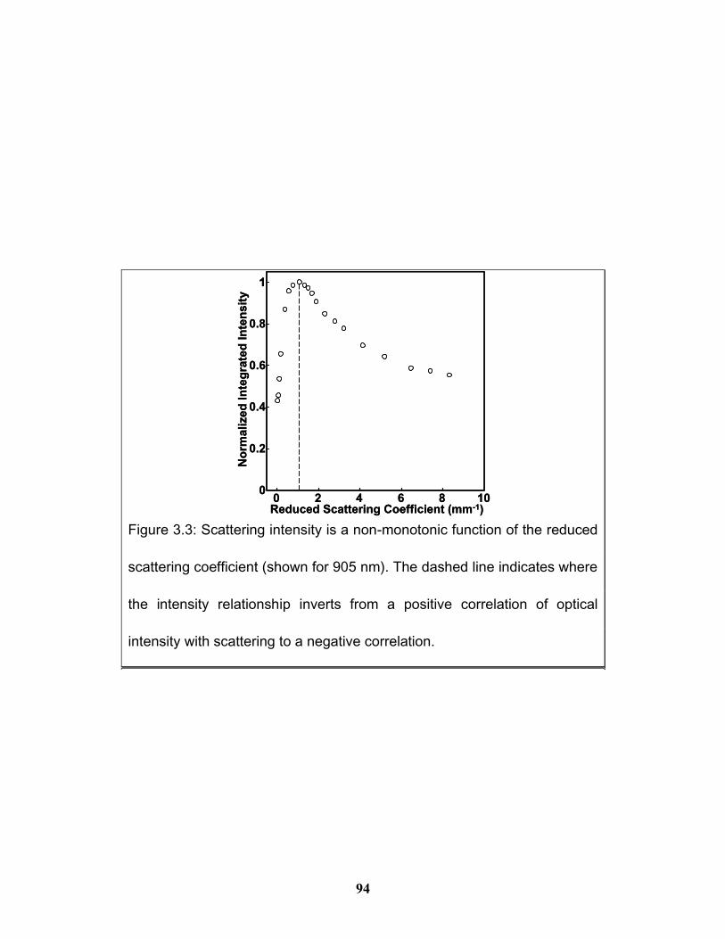
94
0 2 4 6 8 100
0.2
0.4
0.6
0.8
1
Reduced Scattering Coefficient (mm-1)
No
rmali
zed
In
teg
rate
d I
nte
nsit
y
0 2 4 6 8 100
0.2
0.4
0.6
0.8
11
Reduced Scattering Coefficient (mm-1)
No
rmali
zed
In
teg
rate
d I
nte
nsit
y
Figure 3.3: Scattering intensity is a non-monotonic function of the reduced
scattering coefficient (shown for 905 nm). The dashed line indicates where
the intensity relationship inverts from a positive correlation of optical
intensity with scattering to a negative correlation.

95
3.7 Results & Discussion
Time-of-flight profiles were recorded for many scattering levels to
determine the functional scattering range over which the simplified
instrument could measure scattering. Reflectance intensity changes
nonlinearly with scattering, as shown in Figure 3.3. While μs' was less than
1 mm-1 reflectance intensity increased with increasing scattering. When μs'
was greater than 1 mm-1, reflectance intensity decreased with increasing
scattering. In the high scattering domain photons are progressively
constrained to smaller volumes as scattering increases, resulting in
decreasing reflectance intensity at the sampled point. The high scattering
domain was selected for further work. In practice, the reduced scattering
coefficient of human dermis is in the high scattering range.
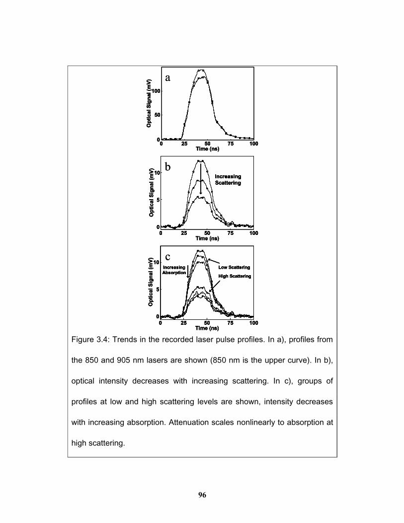
96
0
50
100
Op
tic
al S
ign
al
(mV
)0 25 50 75 100
Time (ns)
0
50
100
Op
tic
al S
ign
al
(mV
)0 25 50 75 100
Time (ns)
a
b
c
0
5
10
Op
tical S
ign
al (m
V)
Increasing
Scattering
0 25 50 75 100Time (ns)
0
5
10
Op
tical S
ign
al (m
V)
Increasing
Scattering
0 25 50 75 100Time (ns)
0
5
10
Op
tic
al S
ign
al
(mV
)
Low Scattering
High Scattering
Increasing
Absorption
0 25 50 75 100Time (ns)
0
5
10
Op
tic
al S
ign
al
(mV
)
Low Scattering
High Scattering
Increasing
Absorption
0 25 50 75 100Time (ns)
0
50
100
Op
tic
al S
ign
al
(mV
)0 25 50 75 100
Time (ns)
0
50
100
Op
tic
al S
ign
al
(mV
)0 25 50 75 100
Time (ns)
a
b
c
0
5
10
Op
tical S
ign
al (m
V)
Increasing
Scattering
0 25 50 75 100Time (ns)
0
5
10
Op
tical S
ign
al (m
V)
Increasing
Scattering
0 25 50 75 100Time (ns)
0
5
10
Op
tic
al S
ign
al
(mV
)
Low Scattering
High Scattering
Increasing
Absorption
0 25 50 75 100Time (ns)
0
5
10
Op
tic
al S
ign
al
(mV
)
Low Scattering
High Scattering
Increasing
Absorption
0 25 50 75 100Time (ns)
Figure 3.4: Trends in the recorded laser pulse profiles. In a), profiles from
the 850 and 905 nm lasers are shown (850 nm is the upper curve). In b),
optical intensity decreases with increasing scattering. In c), groups of
profiles at low and high scattering levels are shown, intensity decreases
with increasing absorption. Attenuation scales nonlinearly to absorption at
high scattering.
97
The instrument was calibrated to measure the reduced scattering
coefficient in the presence of varying absorption. Example temporal data
is shown in Figure 3.4. Both lasers showed similar pulse shapes. As
scattering increased, magnitude of the temporal profiles decreased. As
absorption increased, maximum intensity of the profiles decreased.
Linear regressions were used to estimate the reduced scattering
coefficients using descriptors of the profile calibration data. Time-of-flight
data is determined by simplified descriptors which are less sensitive to
temporal jitter. Descriptors were calculated as described in the methods
section. Linear regressions were used to estimate μs' from each
descriptor. Results of these regressions are listed in Table 3.1. Overall,
using the second moment resulted in the best μs' estimates. This agrees
with previous results.165 Both slope of the falling edge and first moment did
not estimate μs' well. Error in measurement of the mean pulse time
becomes pronounced in wide pulses with a flat maximum intensity. As the
first moment is a measure of mean pulse time, and does not estimate
scattering in the present system. Estimates of μs' were derived from the
second moment. Calibration and validation results for the 850 and 905 nm
lasers using the second moment are shown in Figure 3.5. Coefficients of
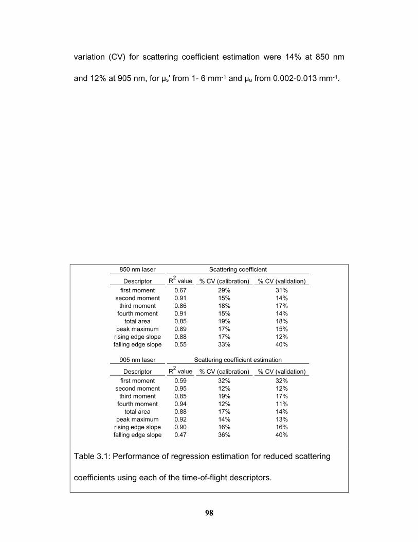
98
variation (CV) for scattering coefficient estimation were 14% at 850 nm
and 12% at 905 nm, for μs' from 1- 6 mm-1 and μa from 0.002-0.013 mm-1.
850 nm laser
Descriptor R2 value % CV (calibration) % CV (validation)
first moment 0.67 29% 31%
second moment 0.91 15% 14%
third moment 0.86 18% 17%
fourth moment 0.91 15% 14%
total area 0.85 19% 18%
peak maximum 0.89 17% 15%
rising edge slope 0.88 17% 12%
falling edge slope 0.55 33% 40%
905 nm laser
Descriptor R2 value % CV (calibration) % CV (validation)
first moment 0.59 32% 32%
second moment 0.95 12% 12%
third moment 0.85 19% 17%
fourth moment 0.94 12% 11%
total area 0.88 17% 14%
peak maximum 0.92 14% 13%
rising edge slope 0.90 16% 16%
falling edge slope 0.47 36% 40%
Scattering coefficient
Scattering coefficient estimation
Table 3.1: Performance of regression estimation for reduced scattering
coefficients using each of the time-of-flight descriptors.
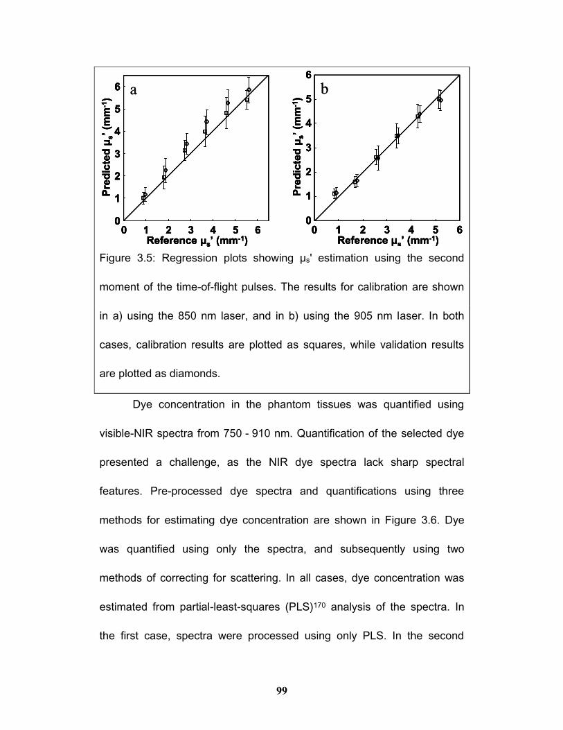
99
Dye concentration in the phantom tissues was quantified using
visible-NIR spectra from 750 - 910 nm. Quantification of the selected dye
presented a challenge, as the NIR dye spectra lack sharp spectral
features. Pre-processed dye spectra and quantifications using three
methods for estimating dye concentration are shown in Figure 3.6. Dye
was quantified using only the spectra, and subsequently using two
methods of correcting for scattering. In all cases, dye concentration was
estimated from partial-least-squares (PLS)170 analysis of the spectra. In
the first case, spectra were processed using only PLS. In the second
0 1 2 3 4 5 60
1
2
3
4
5
6
Reference μs’ (mm-1)
Pre
dic
ted
μs’(m
m-1
)
0 1 2 3 4 5 60
1
2
3
4
5
6
Reference μs’ (mm-1)
Pre
dic
ted
μs’(m
m-1
)
0 1 2 3 4 5 60
1
2
3
4
5
6
Reference μs’ (mm-1)
Pre
dic
ted
μs’(m
m-1
)
0 1 2 3 4 5 60
1
2
3
4
5
6
Reference μs’ (mm-1)
Pre
dic
ted
μs’(m
m-1
)
a b
0 1 2 3 4 5 60
1
2
3
4
5
6
Reference μs’ (mm-1)
Pre
dic
ted
μs’(m
m-1
)
0 1 2 3 4 5 60
1
2
3
4
5
6
Reference μs’ (mm-1)
Pre
dic
ted
μs’(m
m-1
)
0 1 2 3 4 5 60
1
2
3
4
5
6
Reference μs’ (mm-1)
Pre
dic
ted
μs’(m
m-1
)
0 1 2 3 4 5 60
1
2
3
4
5
6
Reference μs’ (mm-1)
Pre
dic
ted
μs’(m
m-1
)
a b
Figure 3.5: Regression plots showing μs' estimation using the second
moment of the time-of-flight pulses. The results for calibration are shown
in a) using the 850 nm laser, and in b) using the 905 nm laser. In both
cases, calibration results are plotted as squares, while validation results
are plotted as diamonds.
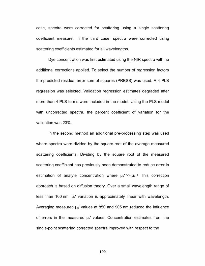
100
case, spectra were corrected for scattering using a single scattering
coefficient measure. In the third case, spectra were corrected using
scattering coefficients estimated for all wavelengths.
Dye concentration was first estimated using the NIR spectra with no
additional corrections applied. To select the number of regression factors
the predicted residual error sum of squares (PRESS) was used. A 4 PLS
regression was selected. Validation regression estimates degraded after
more than 4 PLS terms were included in the model. Using the PLS model
with uncorrected spectra, the percent coefficient of variation for the
validation was 23%.
In the second method an additional pre-processing step was used
where spectra were divided by the square-root of the average measured
scattering coefficients. Dividing by the square root of the measured
scattering coefficient has previously been demonstrated to reduce error in
estimation of analyte concentration where μs' >> μa.1 This correction
approach is based on diffusion theory. Over a small wavelength range of
less than 100 nm, μs' variation is approximately linear with wavelength.
Averaging measured μs' values at 850 and 905 nm reduced the influence
of errors in the measured μs' values. Concentration estimates from the
single-point scattering corrected spectra improved with respect to the
101
0 1 2 3 4 5 60
1
2
3
4
5
6
Reference μs’ (mm-1)
Pre
dic
ted
μs’(m
m-1
)
0 1 2 3 4 5 60
1
2
3
4
5
6
Reference μs’ (mm-1)
Pre
dic
ted
μs’(m
m-1
)
0 1 2 3 4 5 60
1
2
3
4
5
6
Reference μs’ (mm-1)
Pre
dic
ted
μs’(m
m-1
)
0 1 2 3 4 5 60
1
2
3
4
5
6
Reference μs’ (mm-1)
Pre
dic
ted
μs’(m
m-1
)
a b
0 1 2 3 4 5 60
1
2
3
4
5
6
Reference μs’ (mm-1)
Pre
dic
ted
μs’(m
m-1
)
0 1 2 3 4 5 60
1
2
3
4
5
6
Reference μs’ (mm-1)
Pre
dic
ted
μs’(m
m-1
)
0 1 2 3 4 5 60
1
2
3
4
5
6
Reference μs’ (mm-1)
Pre
dic
ted
μs’(m
m-1
)
0 1 2 3 4 5 60
1
2
3
4
5
6
Reference μs’ (mm-1)
Pre
dic
ted
μs’(m
m-1
)
a b
Figure 3.6: Dye concentration estimates with scattering correction. In a),
attenuation spectra of the tissue phantoms are shown plotted to the
attenuation scale (left axis), with the bolded dye spectrum is plotted to the
absorbance scale (right axis). In b), dye concentration was estimated
from uncorrected spectral data with a 4-component PLS model. In c), dye
concentration was estimated from data corrected by measured μs' values
using a 4-component PLS model. In d), dye concentration was estimated
from data corrected by known μs' values using a 3-component PLS model.
Calibration results are plotted as squares, while validation results are
plotted as diamonds.
102
uncorrected spectra. Spectral correction using wavelength-dependent
scattering estimates further improves concentration estimates. From the
PRESS, a 4-term PLS model was again selected. Scatter correction using
a single scattering value correction resulted in a CV of 21%. Using the
measured reduced scattering coefficient improved the CV of dye
concentration estimation in comparison to uncorrected spectra.
In the third method, a multi-wavelength scattering correction was
used. To correct each spectral wavelength, measured attenuation was
divided by the square root of a linear estimate of the μs' at each
wavelength. Known μs' values at 850 and 905 nm were used to generate a
linear estimate of μs' values from 750 to 910 nm. In the ideal case, a linear
trend of scattering with wavelength can be derived from the 2 measured
μs' values using our simplified instrument. Linear scattering estimates are
then applied to spectra over a short wavelength range to correct for
scattering. We show this correction based on known μs' values rather than
directly from the linear estimate of two measured μs'. Extrapolating μs'
values at other wavelengths from a line fitted to two measured points
amplifies measurement error. Future improvements to the instrument
presented here will allow determination of μs' with enough precision to
reliably estimate this linear correction factor from measured μs' values.

103
Dividing measured attenuation spectra by the square root of extrapolated
μs' values improved the validation results. From the PRESS, a 3-term PLS
model was selected. Multiwavelength correction resulted in CV of 17%, a
35% improvement over the uncorrected spectral estimate. In addition to
the improvement in CV, the selected model used fewer terms. A reduction
in the calibration model complexity was possible because scattering had
been corrected.
3.8 Conclusions
Improvements to this time-of-flight system will allow more precise
quantification of μs'. To improve the system, several methods are
suggested. Without modifying the current electronics, a shorter pulse can
be used without decreasing peak optical-power. Detector rise time can be
decreased by increasing the reverse bias applied to the diode. Simplified
electronics can be incorporated to replace the oscilloscope. Unpublished
results illustrate the utility of decimation of the temporal profiles by
electronically windowing the electrical signal from the detector with a
delayed trigger pulse using digital delay lines and a high-speed mixer.
Future improvements in this portable system will allow for quick, robust
multi-wavelength measurement of the reduced scattering coefficients in
highly turbid media such as tissue.
104
It has been shown that the reduced scattering coefficient (μs') in the
range from 1 – 6 mm-1 can be measured at both 850 and 905 nm using a
handheld photon time-of-flight instrument. Analytical descriptors were
used to compress time-of-flight profiles recorded with the portable
instrument. Scattering was then predicted using the descriptors. An
inverse least squares linear regression was used to predict the reduced
scattering coefficient from the second moment. The coefficients of
variation for the measured μs' were shown to be 14.1% at 850 nm, and
11.6% at 905 nm. Furthermore, multiwavelength near-infrared estimates
of dye concentration were improved by 35% using the scattering
correction method. Construction of a miniature device for the
measurement of μs' represents an important step towards quantitative NIR
clinical measurements in turbid media such as tissue. A portable photon
time-of-flight device may prove a convenient alternative to costly
instrumentation for measuring scattering in tissue and other turbid media.
3.9 Acknowledgements
This work was funded by the National Science and Engineering
Research Council (NSERC) of Canada through both research grants and
a PGS scholarship. Additional funding was supplied by the Fonds
Québécois de la Recherche sur la Nature et les Technologies (FQRNT).

105
The authors would also like to thank Karen Esmonde-White for editorial
comments, as well as Texas Instruments, Dallas Semiconductor Corp.,
Intersil, and OSRAM Opto Semiconductors for providing samples and
technical support in the development of the portable photon time-of-flight
device.

106
Chapter 4. Steady-State Diffuse Reflectance
Imaging of an Annular Source Illumination
Pattern for Quantifying Scattering and Absorption
Coefficients of Turbid Media
To correct for scattering using instrumentation, scattering
coefficients can be measured and mathematically corrected for. In
Chapter 3, a photon time-of-flight system for measuring and correcting for
scattering was described. The multi-wavelength scattering coefficient
estimates using the time-of-flight system were shown to improve
quantification by 35%. The time-of-flight method is particularly applicable
for point-measurements.
In this chapter, a novel reflectance imaging system is described,
providing a second method for measuring and correcting scattering in
turbid media. A method is presented here for measuring optical scattering
and absorption properties using steady-state diffuse reflectance imaging
of a ring-shaped laser illumination pattern. By measuring the scattering at
the center of an annular illumination pattern, the scattering coefficient is
measured at the center of the location of interest. Furthermore, this

107
method is amenable to measuring scattering even at scattering levels
much higher than typically present in tissue.
While the photon time-of-flight instrument presented in the previous
chapter is a practical method for measuring and correcting for scattering in
a point-measurement, situations arise where it is preferable to measure
the scattering coefficients at many locations simultaneously. Though
scattering coefficients can be mapped by translating the probe over a
sample, this is not practical in dynamic systems. One example is in
minimally invasive heart surgery (also known as beating-heart surgery)171,
where operations are performed on the beating heart. Assessment and
visualization of tissue oxygen perfusion can help surgeons to monitor
tissue viability. Because the heart is beating it is difficult to mechanically
align the probe and synchronize the measurements to the beating without
introducing errors. Other examples include burn assessment and tumor
removal. In burn assessment it is important to quickly determine which
burns require grafting.98 During the excision of tumors, real-time tissue
classification helps to guide surgeons in removing only cancerous
tissue.106 This is particularly important in brain surgery, where
unnecessarily removing healthy brain matter can have terrible
consequences for the patient. In both of these examples, non-contact
108
imaging can be used to guide medical interventions while avoiding
exacerbation of tissue damage. In this chapter a reflectance imaging
system is described for measuring scattering properties. The imaging
system described here is applicable for measuring scattering in visible and
near-infrared imaging spectroscopy.
4.1 Manuscript
Steady-State Diffuse Reflectance Imaging of an Annular Source
Illumination Pattern for Quantifying Scattering and Absorption Coefficients
of Turbid Media
Authors:
Francis W.L. Esmonde-White and David H. Burns
4.2 Abstract
A novel approach for measuring reduced scattering and absorption
coefficients using imaging of lasers was examined. Rather than detecting
radial reflectance intensity around an incident point source, intensity can
be measured within a small annular pattern projected onto the sample
surface. Reversal of the common source-detector geometry arrangement
allows measurement of absorption and reduced scattering coefficients
from a small surface area. Reduced scattering coefficients were measured
over the range μs' = 0.1 - 40 mm-1, with a coefficient of variation of 12.6%
109
using a ring source & imaging detector optical arrangement. Absorption
coefficients were measured over the range μa = 0 - 0.2 mm-1, with a
coefficient of variation of 11.5%, a 50% reduction of error in comparison
with non-scatter corrected estimates. This method has the potential to
measure scattering coefficients from an array of rings for rapid mapping of
reduced scattering coefficients in spectral reflectance imaging. Ultimately,
the ring source method has the potential to map optical properties for
scatter-correction in spectral imaging.
4.3 Keywords
Scattering, Diffuse Reflectance, Reduced Scattering Coefficient,
Spectral Imaging, Absorption, Turbid Media, Phantom Tissue, Computer
Generated Holograph, Annular Pattern, Ring Pattern, Orbital Angular
Momentum Light, Vortex Light
4.4 Introduction
Diffuse reflectance imaging is a practical modality for recording
spectral information in living systems. Recent examples include imaging of
hemoglobin oxygen saturation,87, 133 assessment of burns,98 and
identification of tumors.106 Tissue is identified or components are
quantified based on the light attenuation, typically, as the logarithmic ratio
of the light remitted without absorbance (reference) to the light remitted
110
with the added molecular species (signal). Using transmission geometries
the reference intensity can be measured directly. However, in diffuse
reflectance imaging spectroscopy the reference intensity can usually not
be measured directly, because it is not possible to measure a blank
(absorption-free sample) with the appropriate scattering level. The
common approach is to instead use reflectance standards or feedback
systems, which correct for variations in the intensity of the light source.27,
172 However, an ideal reference would indicate the reflectance without
added absorption so that attenuation could be directly calculated. When
scattering is not known, it is difficult to determine the appropriate reference
intensity.40 One solution is to measure the scattering so that reference
reflectance intensities can be estimated. Scattering is measured as the
reduced scattering coefficient (μs'), which measures the effective distance
between scattering events and includes the directional dependence of
scattering anisotropy. The absorption coefficient (μa) is the corresponding
measure for describing the absorption of light in terms of inverse
propagation distance rather than absolute pathlength.
Continuous intensity methods have been demonstrated for
measuring optical properties.27 Optical properties are estimated from the
radial intensity pattern of the reflectance around the point source. In
111
particular, diffuse reflectance images of point sources such as from a laser
has been shown for measuring scattering and absorption coefficients.26, 33-
35, 37, 38 Unfortunately, the point source scattering measurements using
imaging techniques require a source detector spacing of many millimetres,
and have poor spatial resolution. Reflectance imaging systems collect
images from a relatively large scale, and range from a half centimetre to
several centimetres. In heterogeneous systems like biological tissue,
scattering and absorption coefficients can vary over a few millimetres.
Spatial resolution and sampling depths are a function of the source-
detector spacing. By reducing the source-detector separation the
scattering coefficient is measured with better spatial resolution.
Scattering coefficients have been measured using fiber-optic
probes with small source-detector spacings. Examples include probes
using a point source and concentric rings of detector fibers,33 as well as
source and detector fibers linearly arranged with total spacings of less
than 2 mm.107 Fiber probes, while having better spatial resolution, are not
ideal for use with spectroscopic imaging because they apply pressure to
the sample surface. Probe pressure can induce temporary physical
deformations, cause changes in the local humidity and optical clearing,142
and disrupt local circulation by pushing blood out of the tissue of interest.
112
Similar problems are observed in fluorescence and Raman
spectroscopy. The ring/disk geometry has been recently reported for
collection of subsurface Raman spectra.173, 174 In particular,
transcutaneous Raman using a similar optical geometry with a ring-
shaped source and centrally-positioned detector bundle has been
reported.173, 174 In spatially-offset Raman spectroscopy, larger source ring
diameters (greater source-detector separation) have been shown to
reduce fluorescence background signal, and improve signal-to-noise ratio
of Raman bands.
Several methods have been reported for the generation of annular
laser patterns.175-183 A single ring can be generated using axicon (axial
conic) lenses or stepped phase-plates.173, 178, 184-186 Arrays of ring patterns
are also possible using holographic interference filters, either as printed
films or using spatial light modulators.187 Printed films have the advantage
of being permanent and inexpensive, while spatial light modulators can be
used to dynamically generate arrays of rings.176, 182, 188, 189 By using arrays
of rings rather than a single ring, concurrent measurement of scattering at
multiple locations should be possible.
We investigated the feasibility of an annular illumination source to
measure scattering at small source-detector separations suitable for an
113
imaging system. A ring patterned laser source and imaging detector were
used to measure reduced scattering and absorption coefficients of tissue
phantoms with known optical properties. Using an annular source pattern
the spatial location over which the scattering coefficient is measured is
small and well-defined, allowing a non-invasive measure of the local
properties with fine spatial resolution. We demonstrate use of annular
patterns with diffuse reflectance imaging to measure the absorption and
reduced scattering coefficients in highly scattering and absorbing tissue
phantoms at a single point, with potential applicability for in-vivo tissue
diagnostics.
4.5 Material and Methods
A diffuse reflectance system for imaging ring-patterned laser was
developed and tested. Image processing methods were developed to
estimate reduced scattering and absorption coefficients of Intralipid/dye
optical tissue phantoms. Details of the optical system, software, and tissue
phantoms are presented in this section.
4.5.1 Instrument Configuration
An annular illumination pattern was generated using a laser, spatial
filter and holographic filter. The experimental configuration is illustrated in
Figure 4.1. A 5 mW Helium-Neon laser beam (Melles-Griot, Carlsbad,
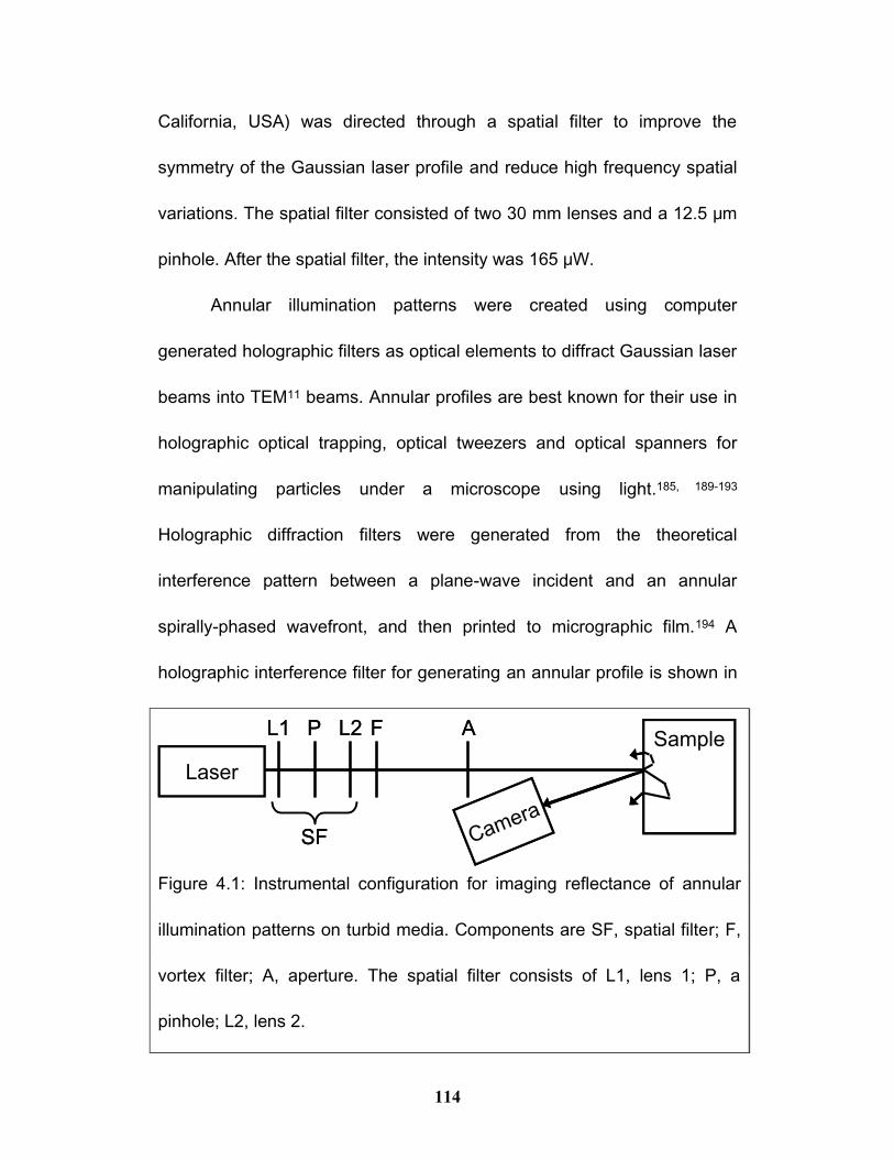
114
California, USA) was directed through a spatial filter to improve the
symmetry of the Gaussian laser profile and reduce high frequency spatial
variations. The spatial filter consisted of two 30 mm lenses and a 12.5 μm
pinhole. After the spatial filter, the intensity was 165 μW.
Annular illumination patterns were created using computer
generated holographic filters as optical elements to diffract Gaussian laser
beams into TEM11 beams. Annular profiles are best known for their use in
holographic optical trapping, optical tweezers and optical spanners for
manipulating particles under a microscope using light.185, 189-193
Holographic diffraction filters were generated from the theoretical
interference pattern between a plane-wave incident and an annular
spirally-phased wavefront, and then printed to micrographic film.194 A
holographic interference filter for generating an annular profile is shown in
Sample
Camera
L1 P L2 F A
Laser
SF
Sample
Camera
L1 P L2 F A
Laser
SF
Figure 4.1: Instrumental configuration for imaging reflectance of annular
illumination patterns on turbid media. Components are SF, spatial filter; F,
vortex filter; A, aperture. The spatial filter consists of L1, lens 1; P, a
pinhole; L2, lens 2.
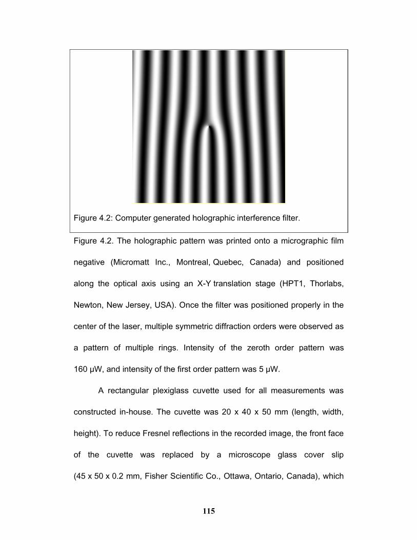
115
Figure 4.2. The holographic pattern was printed onto a micrographic film
negative (Micromatt Inc., Montreal, Quebec, Canada) and positioned
along the optical axis using an X-Y translation stage (HPT1, Thorlabs,
Newton, New Jersey, USA). Once the filter was positioned properly in the
center of the laser, multiple symmetric diffraction orders were observed as
a pattern of multiple rings. Intensity of the zeroth order pattern was
160 μW, and intensity of the first order pattern was 5 μW.
A rectangular plexiglass cuvette used for all measurements was
constructed in-house. The cuvette was 20 x 40 x 50 mm (length, width,
height). To reduce Fresnel reflections in the recorded image, the front face
of the cuvette was replaced by a microscope glass cover slip
(45 x 50 x 0.2 mm, Fisher Scientific Co., Ottawa, Ontario, Canada), which
Figure 4.2: Computer generated holographic interference filter.
116
was trimmed to 40 x 50 mm using a ceramic glass cleaving stone. The
cuvette was positioned 60 cm from the diffraction filter with annular
laser patterns incident at a 90 angle on the surface of the glass cover
slip. Sequentially each ring-shaped diffraction order was selected
individually using a 35 mm linear translation stage and a variable iris with
the diameter adjusted to 1.4 mm. A single diffracted order was permitted
to pass through the aperture. Aperture diameter was held constant over
the experiment while the aperture was linearly translated to select
the proper diffraction order. Results from the second order diffraction
beam are presented.
Diffuse reflectance images were recorded using a 14-bit grayscale
Sony XCD-V50 digital camera (Sony Corporation, Tokyo, Japan) equipped
with a macro lens (Computar M0814-MP, CBC America Corp., Commack,
NY, USA). The camera was positioned with the minimum offset required to
avoid blocking the incident illumination, and was oriented at an angle of
23 to the front surface of the cuvette.
Images were composite exposures created from 25 captured
frames, with each frame having a 10 millisecond exposure time. Resulting
images comprised the average of frames acquired over a 0.8 second time
interval. Reference dark images were subtracted from the averaged
117
sample images to remove structured background resulting from the
camera digitization electronics.
4.5.2 Software
Images were recorded in Matlab (MATLAB, The MathWorks, Inc.,
Natick, MA, USA) using the image acquisition toolbox and the Carnegie
Mellon University DCAM driver. Radial intensity profiles and integrated
annular intensities were measured from each recorded image. Absorption
and reduced scattering coefficients were estimated from integrated
intensities of rings in the reflectance images. Models for estimating the
optical properties of the intralipid phantoms were tested using measured
images of replicate samples to estimate the known optical coefficients.
4.5.3 Phantom Tissue Samples
Tissue phantoms were prepared using Intralipid-20 (Fresenius-
KABI, Uppsala, Sweden) and green dye (Ph. Martin's Juniper Green 12A,
Salis, Florida, USA). Samples were prepared gravimetrically and diluted
with deionised water to a final mass of 100g. A gravimetric sample
preparation method was used since Intralipid adheres to glassware and
can result in inconsistent volume measurements. For each of the 136
phantom tissue samples prepared, scattering and absorption coefficients
were calculated from the known Intralipid and dye concentrations.169
118
Samples were prepared so that solutions had optical properties in a
biologically relevant range with reduced scattering coefficient between
0.1 and 44 mm-1 and absorption coefficient between 0 and 0.34 mm-1.
Samples were prepared in batches of ten to reduce the likelihood of false
correlation due to systematic error. In each batch, sample concentrations
were chosen at random from the predetermined experimental matrix.
Duplicate measurements were made on each Intralipid/dye sample
in random order to minimize the effects of cross contamination. Each
measurement comprised of first rinsing the cuvette three times with the
sample, and then filling the cuvette with the sample. Duplicate
measurements were separated into distinct calibration and validation data
sets, where the first measurement was used in the calibration set, and the
second measurement was used in the validation set.
4.6 Results and Discussion
Diffuse reflectance imaging of annular laser patterns was used to
estimate optical properties. Capacity of the imaging system to measure
optical properties was tested by imaging a series of tissue simulating
phantoms. Diffusion theory suggests an inverse relationship between μs'
and mean photon propagation distance in scattering materials. This
relationship was observed in the measured radial profiles. Different
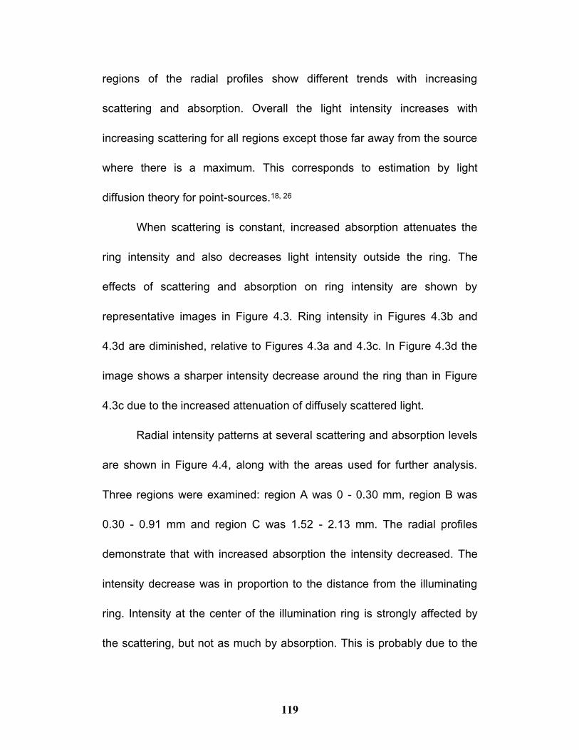
119
regions of the radial profiles show different trends with increasing
scattering and absorption. Overall the light intensity increases with
increasing scattering for all regions except those far away from the source
where there is a maximum. This corresponds to estimation by light
diffusion theory for point-sources.18, 26
When scattering is constant, increased absorption attenuates the
ring intensity and also decreases light intensity outside the ring. The
effects of scattering and absorption on ring intensity are shown by
representative images in Figure 4.3. Ring intensity in Figures 4.3b and
4.3d are diminished, relative to Figures 4.3a and 4.3c. In Figure 4.3d the
image shows a sharper intensity decrease around the ring than in Figure
4.3c due to the increased attenuation of diffusely scattered light.
Radial intensity patterns at several scattering and absorption levels
are shown in Figure 4.4, along with the areas used for further analysis.
Three regions were examined: region A was 0 - 0.30 mm, region B was
0.30 - 0.91 mm and region C was 1.52 - 2.13 mm. The radial profiles
demonstrate that with increased absorption the intensity decreased. The
intensity decrease was in proportion to the distance from the illuminating
ring. Intensity at the center of the illumination ring is strongly affected by
the scattering, but not as much by absorption. This is probably due to the
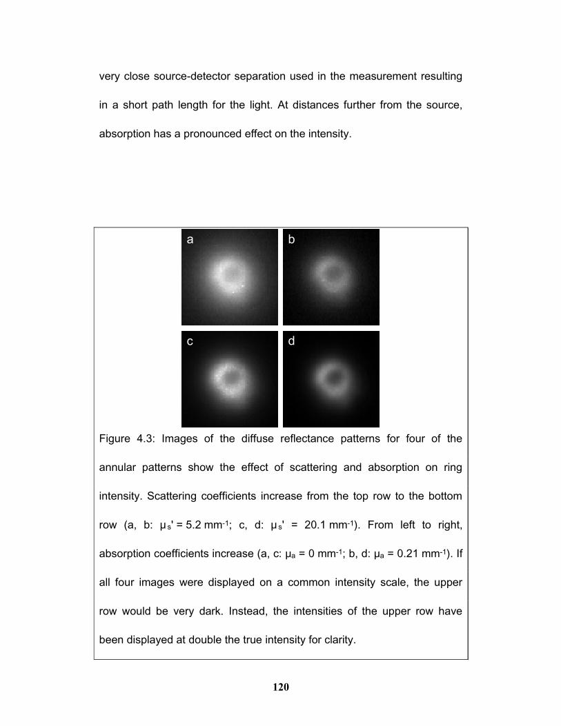
120
very close source-detector separation used in the measurement resulting
in a short path length for the light. At distances further from the source,
absorption has a pronounced effect on the intensity.
a b
c d
a b
c d
Figure 4.3: Images of the diffuse reflectance patterns for four of the
annular patterns show the effect of scattering and absorption on ring
intensity. Scattering coefficients increase from the top row to the bottom
row (a, b: μ s' = 5.2 mm-1; c, d: μ s' = 20.1 mm-1). From left to right,
absorption coefficients increase (a, c: μa = 0 mm-1; b, d: μa = 0.21 mm-1). If
all four images were displayed on a common intensity scale, the upper
row would be very dark. Instead, the intensities of the upper row have
been displayed at double the true intensity for clarity.
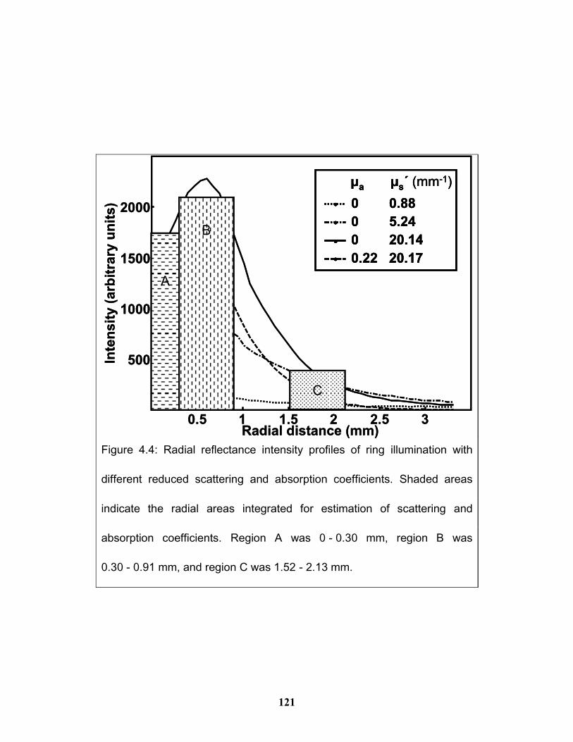
121
0.5 1 1.5 2 2.5 3
500
1000
1500
2000
Radial distance (mm)
Inte
ns
ity (
arb
itra
ry u
nit
s)
A
B
C
0 0.88
0 5.24
0 20.14
0.22 20.17
μa μs´ (mm-1)
0.5 1 1.5 2 2.5 3
500
1000
1500
2000
Radial distance (mm)
Inte
ns
ity (
arb
itra
ry u
nit
s)
A
B
C
0 0.88
0 5.24
0 20.14
0.22 20.17
μa μs´ (mm-1)
0 0.88
0 5.24
0 20.14
0.22 20.17
μa μs´ (mm-1)
Figure 4.4: Radial reflectance intensity profiles of ring illumination with
different reduced scattering and absorption coefficients. Shaded areas
indicate the radial areas integrated for estimation of scattering and
absorption coefficients. Region A was 0 - 0.30 mm, region B was
0.30 - 0.91 mm, and region C was 1.52 - 2.13 mm.

122
4.6.1 Estimation of Reduced Scattering Coefficient
Reflectance intensities within radial regions A, B, and C were
integrated to estimate absorption and reduced scattering coefficients of
the turbid media. As shown in Figure 4.5, reduced scattering coefficients
were estimated from the integrated intensities of regions A and B using an
inverse least squares calibration of 131 samples. The weighting of the
signal for region A was negative in the final calibration and approximately
0 10 20 30 400
10
20
30
40
Reference Reduced Scattering
Coefficient (mm-1)
Pre
dic
ted
Sc
att
eri
ng
Co
eff
icie
nt
(mm
-1)
0 10 20 30 400
10
20
30
40
Reference Reduced Scattering
Coefficient (mm-1)
Pre
dic
ted
Sc
att
eri
ng
Co
eff
icie
nt
(mm
-1)
a b
0 10 20 30 400
10
20
30
40
Reference Reduced Scattering
Coefficient (mm-1)
Pre
dic
ted
Sc
att
eri
ng
Co
eff
icie
nt
(mm
-1)
0 10 20 30 400
10
20
30
40
Reference Reduced Scattering
Coefficient (mm-1)
Pre
dic
ted
Sc
att
eri
ng
Co
eff
icie
nt
(mm
-1)
a b
Figure 4.5: Scattering calibration and validation, as estimated from
intensity at the disc A and the ring B. In a) calibration estimates are
shown, and in b) validation estimates are shown. No differences were
observed between calibration and validation estimates.
Validation CV = 12.6% and r2 = 0.97 where μ s' < 40 mm-1, and
μa < 0.3 mm-1 for 131 samples.
123
5.8 times greater than the weighting for region B. The magnitudes of the
coefficients are approximately equivalent to the ratio of the number of
pixels in the respective regions, suggesting a derivative relationship
between the regions is linearly proportional to the scattering coefficient.
Using the linear model with two terms, reduced scattering coefficients
were then estimated for the calibration and validation data sets. Scattering
coefficients in the validation data set (n=131) were estimated with a
coefficient of variation (CV) of 12.6% and a coefficient of determination (r2)
of 0.97. The results are very encouraging. No direct comparisons can be
made with results from other studies because none have been
demonstrated over such a large range of scattering and absorption
coefficients. Two similar works have been published involving imaging
measurements of scattering over short distances. In the first, Kienle et al.
reported calibrations of optical properties by imaging radial reflectance
patterns 2 to 12 mm from the source.35 Optical properties of 13 tissue-
simulating phantoms were determined over an absorption range of
0.002 < μa < 0.1 mm-1 with a root-mean-square error of ±13.6%, and over
a scattering range of 0.5 < μs' < 2.5 mm-1 with a root-mean-square error of
2.6%. Pham et al. reported calibrations of optical properties from
hyperspectral images of radial reflectance patterns 0.5 to 2.5 mm from the
124
source.37 Optical properties of 15 tissue-simulating phantoms were
determined over an absorption range of 0.001 < μa < 0.2 mm-1 with a root-
mean-square error of ± 12%, and over a scattering range of
0.3 < μs' < 2.5 mm-1 with a root-mean-square error of 4%. In the present
work, scattering coefficients were determined over a much wider range of
reduced scattering coefficients, and shorter source-detector separation
distances.
Even with short source-detector separations the absorption
becomes significant with very high scattering levels. We found that the
scattering calibration deviates from linearity when μs' > 30 mm-1, and may
be a consequence of using only two terms in the calibration model.
Estimations at higher scattering levels may be improved by taking into
account additional radial regions or by using a nonlinear calibration model.
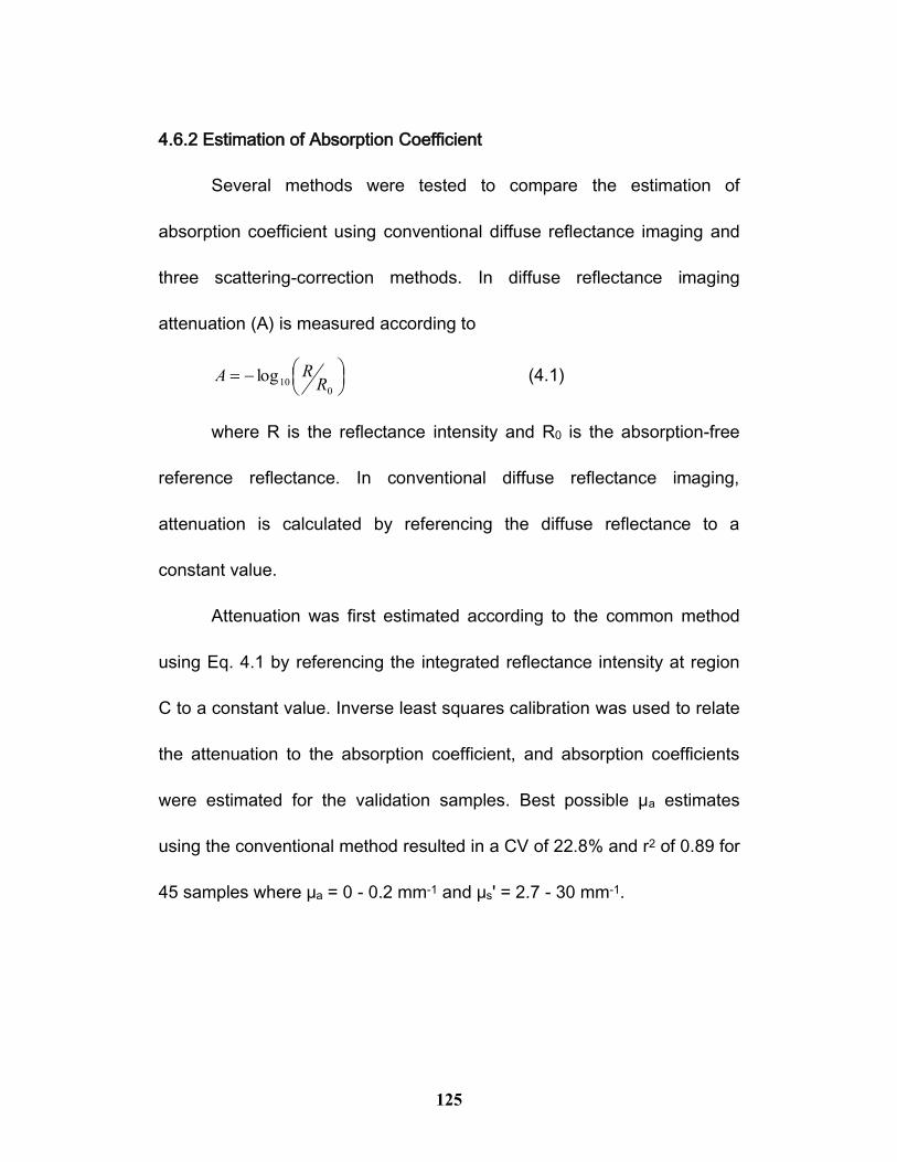
125
4.6.2 Estimation of Absorption Coefficient
Several methods were tested to compare the estimation of
absorption coefficient using conventional diffuse reflectance imaging and
three scattering-correction methods. In diffuse reflectance imaging
attenuation (A) is measured according to
0
10logR
RA (4.1)
where R is the reflectance intensity and R0 is the absorption-free
reference reflectance. In conventional diffuse reflectance imaging,
attenuation is calculated by referencing the diffuse reflectance to a
constant value.
Attenuation was first estimated according to the common method
using Eq. 4.1 by referencing the integrated reflectance intensity at region
C to a constant value. Inverse least squares calibration was used to relate
the attenuation to the absorption coefficient, and absorption coefficients
were estimated for the validation samples. Best possible μa estimates
using the conventional method resulted in a CV of 22.8% and r2 of 0.89 for
45 samples where μa = 0 - 0.2 mm-1 and μs' = 2.7 - 30 mm-1.
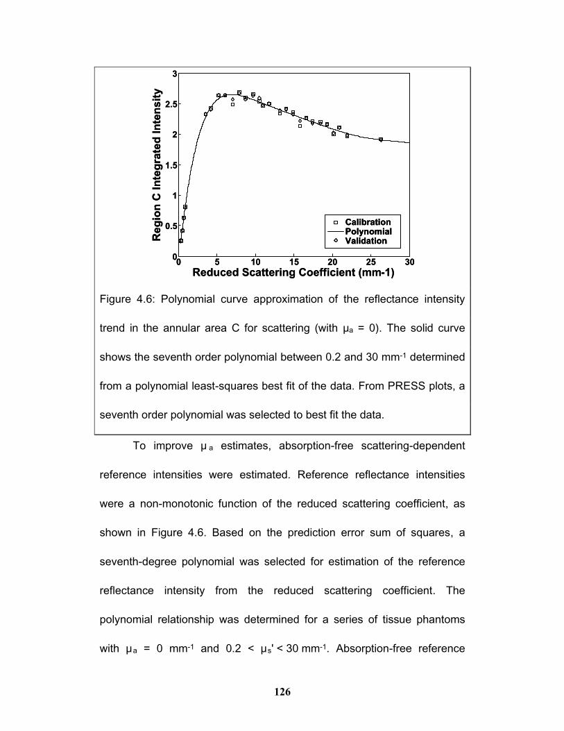
126
To improve μ a estimates, absorption-free scattering-dependent
reference intensities were estimated. Reference reflectance intensities
were a non-monotonic function of the reduced scattering coefficient, as
shown in Figure 4.6. Based on the prediction error sum of squares, a
seventh-degree polynomial was selected for estimation of the reference
reflectance intensity from the reduced scattering coefficient. The
polynomial relationship was determined for a series of tissue phantoms
with μa = 0 mm-1 and 0.2 < μs' < 30 mm-1. Absorption-free reference
0 5 10 15 20 25 300
0.5
1
1.5
2
2.5
3
Reduced Scattering Coefficient (mm-1)
Re
gio
n C
In
teg
rate
d I
nte
ns
ity
CalibrationPolynomialValidation
0 5 10 15 20 25 300
0.5
1
1.5
2
2.5
3
Reduced Scattering Coefficient (mm-1)
Re
gio
n C
In
teg
rate
d I
nte
ns
ity
CalibrationPolynomialValidation
CalibrationPolynomialValidation
Figure 4.6: Polynomial curve approximation of the reflectance intensity
trend in the annular area C for scattering (with μa = 0). The solid curve
shows the seventh order polynomial between 0.2 and 30 mm-1 determined
from a polynomial least-squares best fit of the data. From PRESS plots, a
seventh order polynomial was selected to best fit the data.
127
reflectance (R0) was then estimated using the polynomial function and the
reduced scattering coefficient measured for each sample as described
above. Corrected attenuation was then calculated from Eq. 4.1. Inverse
least squares calibration was used to relate the attenuation to the
absorption coefficient, results are shown in Figure 4.7a. Using this method
and an independent set of validation samples were estimated with a CV of
15.6% and r2 of 0.95 for 45 samples where 0 < μa < 0.2 mm-1 and
2.7 < μs' < 30 mm-1.
Integrated reflectance intensity can be estimated using the diffusion
equation where:26
(4.2)
and 2/1'3 saaeff , '' /' sasa , and 1
0 1
sgz . By
simplifying and substituting Eq. 4.2 into Eq. 4.1, the relationship between
attenuation and absorption coefficient can be simplified to:
(4.3)
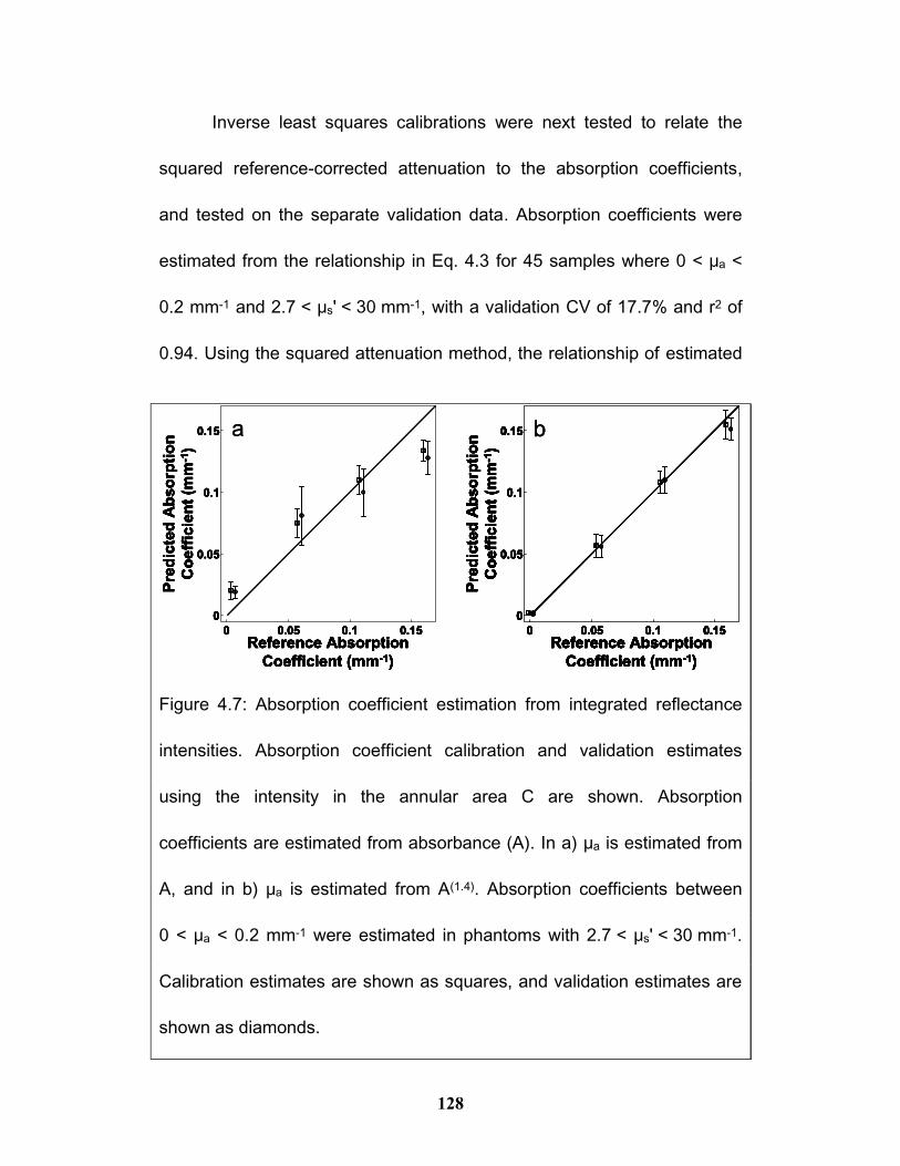
128
Inverse least squares calibrations were next tested to relate the
squared reference-corrected attenuation to the absorption coefficients,
and tested on the separate validation data. Absorption coefficients were
estimated from the relationship in Eq. 4.3 for 45 samples where 0 < μa <
0.2 mm-1 and 2.7 < μs' < 30 mm-1, with a validation CV of 17.7% and r2 of
0.94. Using the squared attenuation method, the relationship of estimated
a
0 0.05 0.1 0.15
0
0.05
0.1
0.15
Reference Absorption
Coefficient (mm-1)
Pre
dic
ted
Ab
so
rpti
on
Co
eff
icie
nt
(mm
-1)
0 0.05 0.1 0.15
0
0.05
0.1
0.15
Reference Absorption
Coefficient (mm-1)
Pre
dic
ted
Ab
so
rpti
on
Co
eff
icie
nt
(mm
-1)
0 0.05 0.1 0.15
0
0.05
0.1
0.15
Reference Absorption
Coefficient (mm-1)
Pre
dic
ted
Ab
so
rpti
on
Co
eff
icie
nt
(mm
-1)
b
0 0.05 0.1 0.15
0
0.05
0.1
0.15
Reference Absorption
Coefficient (mm-1)
Pre
dic
ted
Ab
so
rpti
on
Co
eff
icie
nt
(mm
-1)
0 0.05 0.1 0.15
0
0.05
0.1
0.15
Reference Absorption
Coefficient (mm-1)
Pre
dic
ted
Ab
so
rpti
on
Co
eff
icie
nt
(mm
-1)
0 0.05 0.1 0.15
0
0.05
0.1
0.15
Reference Absorption
Coefficient (mm-1)
Pre
dic
ted
Ab
so
rpti
on
Co
eff
icie
nt
(mm
-1)
Figure 4.7: Absorption coefficient estimation from integrated reflectance
intensities. Absorption coefficient calibration and validation estimates
using the intensity in the annular area C are shown. Absorption
coefficients are estimated from absorbance (A). In a) μa is estimated from
A, and in b) μa is estimated from A(1.4). Absorption coefficients between
0 < μa < 0.2 mm-1 were estimated in phantoms with 2.7 < μs' < 30 mm-1.
Calibration estimates are shown as squares, and validation estimates are
shown as diamonds.
129
absorption to reference absorption remained nonlinear. The nonlinearity
may be due to the approximations made in the derivation of Equations 4.2
and 4.3, or due to the non-zero absorption of light by Intralipid. The
diffusion approximation uses a truncation of terms representing anisotropy
in a Taylor series expansion. Equations 4.2 and 4.3 are based on the
diffusion approximation, and so the relationships are not exact for highly
forward scattering media.
To correct the nonlinearity in the attenuation-absorption coefficient
relationship, non-integer exponents were tested. From the non-negative
experimental attenuation values, the optimal exponent relating attenuation
to absorption coefficient was calculated to be 1.4, at which r2 was
maximized and CV minimized. Using this experimentally determined
exponent, inverse least squares calibrations were used to relate A1.4 to μa.
Validation results are shown in Figure 4.7b, in which absorption
coefficients were estimated for 45 independent validation samples with a
CV of 11.5% and an r2 of 0.96 where 0 < μa < 0.2 mm-1 and 2.7 < μ
s' < 30 mm-1. Using scattering correction with the scattering coefficients
measured by ring illumination improves both the precision and linearity of
estimated absorption coefficients as compared to conventional
approaches. Using the scattering-estimated reference when determining
130
the absorption coefficient, we observed a 30% reduction in CV and an
increase in linearity from an r2 of 0.89 to 0.95. Using the theoretically-
derived squared attenuation, validation performance was slightly lower,
however with the experimentally determined exponential relationship of
A1.4∝μa, the CV was decreased by 50% and the r2 further increased to
0.96.
4.7 Conclusion
Results show that annular illumination is a viable approach to
measuring tissue optical properties. Light diffusion theories, developed for
point-sources, can be applied to ring sources. Light intensities of the ring-
shaped laser and at distances from the ring were measured using a
steady-state diffuse reflectance imaging system. Absorption and reduced
scattering coefficients were quantified over short distances, and the
quantification results indicate good agreement with previous studies.
Optical properties of Intralipid/dye phantom tissue samples with
0 < μa < 0.3 mm-1 and 0 < μ s' < 40 mm-1 were quantified. Reduced
scattering coefficients were estimated with a CV of 12.6% and r2 of 0.97
using intensities measured over a disc 0.30 mm in radius, and a ring from
0.30 - 0.91 mm. Absorption coefficients were estimated with a CV of
131
11.5% and r2 of 0.96 using intensities measured over a ring from
1.52 - 2.12 mm.
Several features of this method are useful for non-invasive
spectroscopic tissue imaging. First, the measurements are made without
applying pressure to the sample. When pressure is applied to tissue
optical properties can change due to regional blood distribution and tissue
compression.142 Non-contact measurements reduce these sources of
pressure-induced variance. Second, the ring-shaped incident pattern
spreads light over a ring instead of focusing the laser to a single point.
Risk of tissue damage is reduced because incident laser power is spread
over a larger area than for a focused point-source of equivalent intensity.
For surgical applications, a ceiling mounted imaging device may be
practical. With increased collection distances, the f-number of the
collection optics becomes very large, and an increase of the source
intensity would be required. Higher laser intensities can be safely used
with annular patterns as compared to a focused Gaussian laser for
imaging scattering coefficients with an equivalent spatial resolution.
Increased source power also translates to shorter acquisition times or
increased signal-to-noise levels. Third, optical scattering properties are
132
measured within a small illumination ring, leading to high spatial resolution
of the measured properties.
Grier has previously reported using arrays of optical rings for optical
trapping of small particles.189 A potential extension of this method is to
generate an array of rings using an active optical element such as a
spatial light modulator. Dynamic generation of annular illumination
patterns could allow simultaneous mapping of scattering coefficients over
a large surface.
4.8 Acknowledgements
This work was funded by the National Science and Engineering
Research Council (NSERC) of Canada through both research grants and
a PGS scholarship. Additional funding was supplied by the Fonds
Québécois de la Recherche sur la Nature et les Technologies (FQRNT).
The authors would also like to thank Matthew Schulmerich for feedback,
Karen Esmonde-White for editorial comments, and Micromatt Inc.
(Montreal, Canada) for providing technical help in printing the microfilm
optical filters.

133
Chapter 5. Generic Parsimony in Genetic
Algorithms for Selecting Spectral Processing
Models in Regression and Classification
Quantification in turbid media can be augmented by measuring
scattering coefficients in addition to spectra. The practical point-source
and imaging methods for measuring scattering shown in Chapters 3 and 4
allow for quantification improvements of 35% and 50% over typical
methods. Instead of using novel instruments, it is possible to improve
quantification using improved data processing methods with conventional
instrumentation.
In this chapter a novel method for finding parsimonious
spectroscopic data processing models is presented. Spectroscopic
measurements of turbid media are often difficult to interpret. Furthermore,
spectral properties of samples may change over time, requiring that
models be periodically revised. Genetic algorithms have been used to
simplify the process of selecting data processing models, with particular
applications for processing spectra measured from turbid media.
Development of parsimonious models has previously required operator
intervention in the crafting of custom penalty weightings. Generic
134
parsimony penalty functions are presented here for the automated
selection of optimal models using genetic algorithms. Matlab source code
for the genetic algorithm described in this chapter is provided in Appendix
C. To understand the use of parsimony in genetic algorithms, an
introduction is given prior to the main body of this chapter.
5.1 Genetic Algorithms
One approach to building optimal processing models uses genetic
algorithms to automatically select regression and classification models.
Genetic algorithms are nonlinear search algorithms based loosely on
simulated evolution.195 Pre-processing options and wavelengths of interest
are coded as a string of binary digits analogous to a genetic code, and
optimal models are selected by the GA using a simulated-evolution
method akin to 'survival of the fittest'. Model selection is a highly nonlinear
process, where selecting slightly different options may result in vastly
different model fitness outcomes. Pre-processing options and useful
wavelengths can be automatically suggested by genetic algorithms, and
expert knowledge is only required in the final selection and application of
the models. This allows the expert to reduce time spent in developing
processing methods by trial and error. One disadvantage of using genetic
algorithms is that the selected processing models can be difficult to
135
interpret, because no justification is provided by the algorithm as to why
particular pre-processing options and wavelengths are selected. In genetic
algorithms the choice of an optimal fitness function is crucial, and should
include some form of parsimony.
Parsimony is a term meaning to spare complexity. Most commonly
parsimony is used to describe the application of Occam's razor. This
principle plays an important role in building data processing models. One
danger in automated method development is the adoption of complex
models which are adapted to noise in the calibration sample, and perform
poorly with independent validation and test samples. Model complexity
can also have a secondary cost, because complex methods also require
unnecessarily complex instrumentation. While the cost of analytical
instrumentation is not often prohibitive in research, methods should be
oriented towards maximum simplicity to reduce time and cost of routine
testing in anticipation of usage under non-laboratory conditions.
Development of simplified methods and simplified instrumentation can be
guided by automated methods which take into account parsimony.
Genetic algorithms which do not penalize for model complexity will evolve
very complex models to fit the data as closely as possible. To avoid this,
various penalties or constraints are typically applied to model fitness to
136
emphasize the utility of smaller models. Because the success of genetic
algorithms are based on evaluations of processing model fitness, the
selection of appropriate fitness functions and associated parsimony
penalties are very important.
Fitness functions for regression and classification genetic
algorithms vary widely. Standard error104 and root mean square error196-200
are often used to evaluate regression model fitness. Regression error is
continuous and suitable for genetic algorithm optimizations. Classification
fitness functions used in genetic algorithms based on classification
accuracy have been reported.201-204 In this chapter, generic parsimony
penalties based on root mean square regression error and Bayesian
classification error are examined.
5.2 Manuscript
Generic Parsimony in Genetic Algorithms for Selecting Spectral
Processing Models in Regression and Classification
Authors:
Francis W.L. Esmonde-White and David H. Burns
5.3 Abstract
Genetic algorithms have been used to develop models for
processing spectroscopic data. Genetic algorithms are able to search a
137
very large number of possible model types and identify models for closer
examination. Unfortunately, very complex models are often developed and
techniques for limiting model complexity must be optimized for each
particular application in regression and classification. A generalized
approach for implementing parsimony was explored by comparing results
from a series of regression and classification genetic algorithms
incorporating different penalization criteria. Regression models were
selected using mean square error and parsimony penalties. Classification
models were selected using log-likelihood of correct classification and
parsimony penalties. Penalties were based on the number of degrees of
freedom, by taking into consideration the number of selected wavelengths
and enabled pre-processing steps. Parsimony penalties were found to
improve the regression and classification models selected by the genetic
algorithm. In particular, the genetic algorithm incorporating parsimony
located a simple regression processing method with a lower cross
validation error than the optimal expert-developed processing method.
5.4 Keywords
genetic algorithm, regression, quantification, classification,
wavelength selection, pre-processing option selection

138
5.5 Introduction
Spectroscopic measurements are used for non-destructive
quantification and classification. However, development of robust spectral
processing models can be extremely complex. Spectral data acquired
from industrial processes, biological fluids, and biological tissues include
significant variability from spectral backgrounds and interference from
chemical species other than the analyte of interest. Physical analytical
methods such as enzymatic digestion and chromatographic purification
can sometimes be used to prepare samples for analysis. However, extra
sample preparation steps are costly, require time, and may increase the
uncertainty in the spectroscopic measurement by virtue of increased
sample handling. Methods for processing spectral data are often a
practical alternative, where analytes are measured without pre-treatment
steps. Moreover, computational costs are low, even for very complex
spectral data analysis. Processing models are composed of
pre-processing steps, such as background correction or smoothing, in
conjunction with selection of wavelength regions that will best quantify or
classify samples. Despite advances in computer hardware, method
development for regression or classification based on spectroscopic data
is still limited by the selection of pre-processing steps and optimal

139
wavelength for analysis. Optimization of data processing models is an
iterative process and relies partly on chance. Additionally, the
spectroscopic background and sample chemical compositions may
change over time, requiring experts to periodically revise processing
models.
Instead of developing processing methods manually through trial
and error, search algorithms are used to select data processing models.
Algorithms for optimizing processing methods must search a large,
irregular set of solutions. Over the past decade genetic algorithms have
been increasingly used to automate selection of regression and
classification models for analysis of spectroscopic data.105, 200-202, 205-212
Genetic algorithms are used to automatically identify processing models,
requiring expert knowledge only for selection and application of the final
model. A major challenge in using genetic algorithms is the
implementation of an appropriate parsimony function.
Complex models generally fit calibration data more closely than do
simple models. Because of this, unconstrained automatic model selection
algorithms will preferentially select complex models over simple models.
However, complex models also adapt to fit noise in calibration data and
perform poorly when validated against independent test data. It is
140
important to use fitness evaluation functions that incorporate penalties to
balance data fitting against model complexity.213 Parsimony is usually
implemented as a penalty based on model size. Either system-specific or
general parsimony penalties can be implemented. System-specific penalty
weights require significant effort to develop and small changes in the
assigned weightings can have a dramatic effect on model selection.212
Alternately, generalized penalties can be implemented using the number
of degrees of freedom in the model.214-216 Degrees of freedom are one
method for the representation of model complexity, and are calculated by
subtracting the number of coefficients used for processing data from the
total number of observations within the data.
In this manuscript, several generalized penalties are examined for
parsimonious model selection for regression and classification. Parsimony
is implemented based on the model evaluation functions for regression
and classification. To evaluate regression model fitness, standard error
and root mean square error are commonly used.196-200 Regression error is
continuous and suitable for genetic algorithm optimizations. Different
penalty functions based on regression error were examined using in-vivo
diffuse reflectance NIR spectra of human fingernails to estimate lactate
concentration.95 To evaluate classification model fitness, classification
141
success rate (also known as accuracy) is commonly used.201-204 Success
rates are determined as a ratio of the number of samples correctly
identified to the number of samples incorrectly classified.217 Precision of
the success rate is dependent on the number of samples in the data. In
small data sets the success rate is imprecise and cannot be used to
discriminate between processing models with small performance
differences. This drawback is problematic when developing methods for
classification of biomedical samples, where the number of samples is
limited by cost or availability of patients. An alternate approach was
developed using Bayesian probabilities to classify samples and a Gibbs
entropy measure to evaluate processing model fitness.218-220 Parsimony
criteria from information-theory based on penalization of log-likelihood
values were then applied to guide model development.216 Development of
models using entropy-based classification fitness parsimony was tested
with attenuated total reflectance mid-infrared spectra of starches.221
5.6 Methodology
To test the influence of parsimony on model selection, a genetic
algorithm was developed and tested with various parsimony functions.
The genetic algorithm consists of two portions: a pseudo-evolution based
optimization algorithm and a function for evaluation of the fitness of

142
processing models. Fitness functions were developed for regression and
classification of samples using spectral data. Effects of parsimony were
tested by examining the performance of the genetic algorithm when using
different parsimony criteria as applied to spectral data.
5.6.1 Software
A non-generational genetic algorithm was developed in Matlab (The
Mathworks, Inc., Natick, MA) using genetic algorithm techniques as
outlined by Luke.222 Non-generational genetic algorithms are useful
because they immediately incorporate optimal solutions into the
development of new population members as they are discovered, rather
than waiting until an entire generation has been processed. Different
fitness functions were implemented in order to evaluate regression models
and classification models, where in all cases the underlying genetic
algorithm was identical. Effects of parsimony on model selection were
examined by comparing several parsimony implementations for regression
and classification fitness functions. All fitness functions used a cross-
validation approach to measuring model fitness, where data from k
samples was divided into n groups of spectra. Each of the n groups was in
turn used as validation data while the remaining n-1 groups were used as
143
calibration data. Results from the n evaluation steps were combined in
order to approximate the model fitness.
Steps used in the genetic algorithm were:
1. Randomly initialize the initial population
2. Evaluate the fitness of all population members
3. Generate a new population member using crossover and mutation
4. Evaluate the new population member
5. Selectively replace one population member
6. Repeat steps 3 - 5 for the specified number of evolution steps
To evaluate the fitness of each genetic algorithm population
member, each model was tested using a fitness function. Data was first
pre-processed according to selected options. Next, coefficients for a linear
regression calibration were determined using the wavelengths selected
from the calibration data. Properties of the validation data were estimated
using the coefficients calculated from the calibration data. For
classification, an extra step was included, using the score calculated from
the regression to estimate the sample class using a Bayesian probability
measure for classification.
144
5.6.2 Pre-processing Options and Score Calculation
Each solution vector developed by the GA coded a series of steps
for pre-processing the spectral data. A maximum of six pre-processing
steps were permitted in any processing model. Common pre-processing
options were explored, including: removing linear trends in data (using the
Matlab function 'detrend'), boxcar smoothing, taking the discrete first
difference93, discrete second difference93, Haar wavelet transform211,
mean centering, autoscaling, unit scaling, range scale, intensity scaling,
area normalizing, and vector normalization. Processing models also
included extra parameters for each pre-processing option. Two
parameters were generated for each pre-processing option (though used
only with certain pre-processing steps): smoothing window, and gap for
computation of differences. Smoothing windows were required by the
boxcar smoothing and discrete difference methods. Noise in
measurements may be reduced by smoothing the data, and a smoothing
window parameter specifies the number of spectral values to be used in
calculating averages. Derivatives were calculated by taking the difference
between data points separated by a number of values specified by the gap
parameter. Calibration and validation data were separately pre-processed
145
for each cross-validation permutation step according to the sequence and
options specified in the processing model.
From the vector of selected wavelengths in the pre-processing
spectral data, an inverse least squares regression model was developed
from the calibration set. Score values estimating the known property
(either the concentration or sample class) were calculated for each sample
in the calibration and validation sets using the inverse least squares
regression model.
5.6.3 Binary Representation of Processing Models
Spectral processing models, pre-processing options and
wavelengths of interest were encoded in a string of binary digits. In the
first portion six pre-processing steps were encoded. Each pre-processing
step was encoded in a sequence of 14 binary digits, using a Gray coding
scheme to encode the various required parameters. The bitstring
encoding scheme is shown in Figure 5.1. In each pre-processing string:
4 bits were used to select the type of pre-processing function to be
applied, 1 bit was used to select the dimension along which the step
should be performed (when applicable), 5 bits to encode the width of the
smoothing window as an integer number between 1 and 32, and the next
4 bits to encode the derivative gap as an odd integer between 3 and 33. In
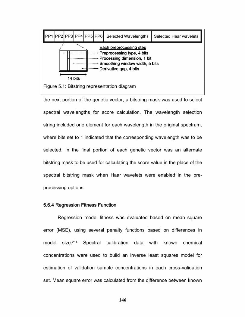
146
the next portion of the genetic vector, a bitstring mask was used to select
spectral wavelengths for score calculation. The wavelength selection
string included one element for each wavelength in the original spectrum,
where bits set to 1 indicated that the corresponding wavelength was to be
selected. In the final portion of each genetic vector was an alternate
bitstring mask to be used for calculating the score value in the place of the
spectral bitstring mask when Haar wavelets were enabled in the pre-
processing options.
5.6.4 Regression Fitness Function
Regression model fitness was evaluated based on mean square
error (MSE), using several penalty functions based on differences in
model size.214 Spectral calibration data with known chemical
concentrations were used to build an inverse least squares model for
estimation of validation sample concentrations in each cross-validation
set. Mean square error was calculated from the difference between known
PP1 Selected Wavelengths Selected Haar waveletsPP2 PP3 PP4 PP5 PP6
14 bits
Preprocessing type, 4 bits
Processing dimension, 1 bit
Smoothing window width, 5 bits
Derivative gap, 4 bits
Each preprocessing step
PP1 Selected Wavelengths Selected Haar waveletsPP2 PP3 PP4 PP5 PP6PP1 Selected Wavelengths Selected Haar waveletsPP2 PP3 PP4 PP5 PP6
14 bits
Preprocessing type, 4 bits
Processing dimension, 1 bit
Smoothing window width, 5 bits
Derivative gap, 4 bits
Each preprocessing step
Preprocessing type, 4 bits
Processing dimension, 1 bit
Smoothing window width, 5 bits
Derivative gap, 4 bits
Each preprocessing step
Figure 5.1: Bitstring representation diagram
147
and estimated validation sample concentrations. Fitness penalty functions
incorporated combinations of the number of pre-processing steps and
number of wavelengths selected to reduce the number of degrees of
freedom when computing MSE. For reference, an initial series of model
selection runs applied no model-size penalties. Next, degrees of freedom
were decreased by the number of wavelengths included in the model.
Finally, both the count of pre-processing options and number of
wavelengths were used to penalize the MSE. Statistical distributions of
model complexity based on the number of selected wavelengths have
previously been examined in this way. However, assignment of penalties
based on pre-processing options is not as well developed. For example,
consider the use of a smoothing function. Using a smoothing function with
a window of 3 effectively triples the number of wavelengths having
influence on the regression model estimates. However, model complexity
using smoothing does not increase by the same amount as it would with
inclusion of three times the number of wavelengths for regression because
of spectral collinearity. The statistical distribution and degrees of freedom
are not well defined for use with various pre-processing options. Each
selected pre-processing option constrains the model, and we opted to
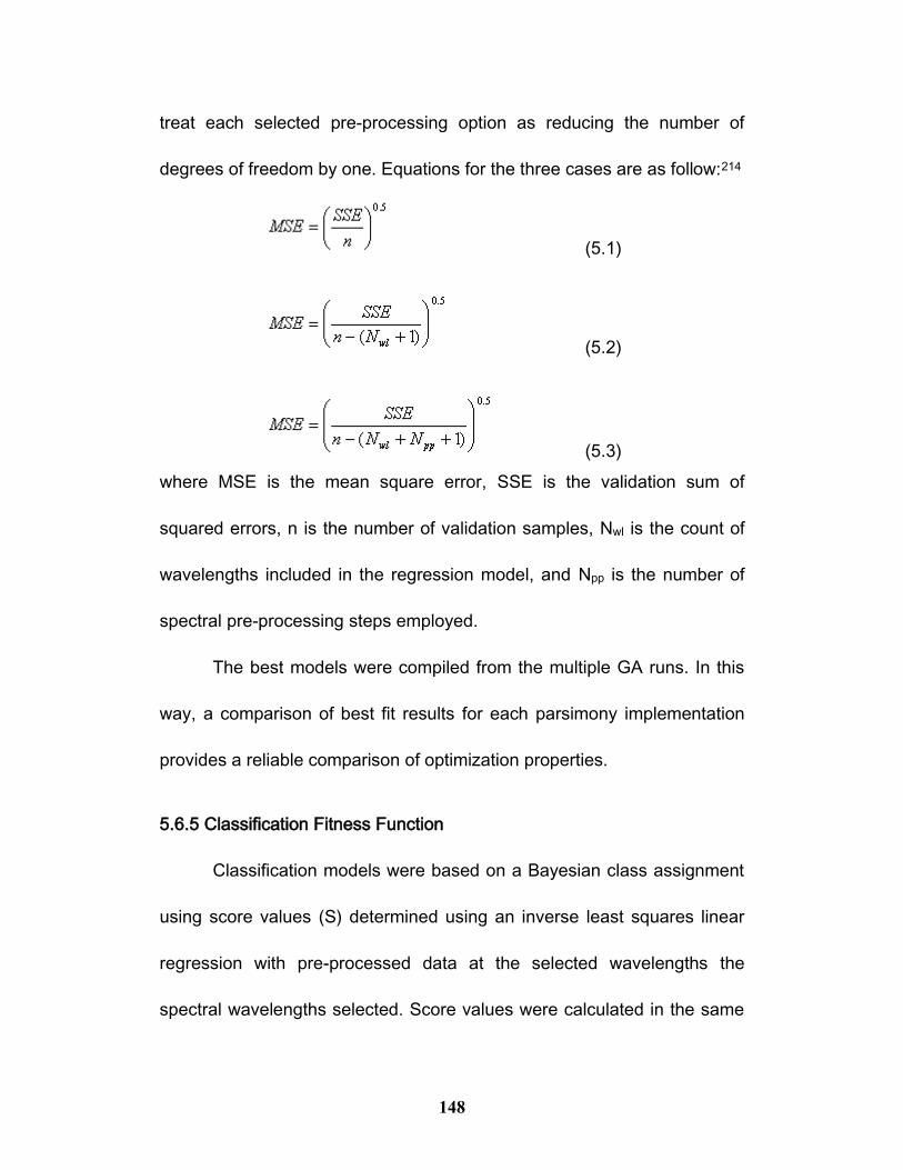
148
treat each selected pre-processing option as reducing the number of
degrees of freedom by one. Equations for the three cases are as follow:214
(5.1)
(5.2)
(5.3)
where MSE is the mean square error, SSE is the validation sum of
squared errors, n is the number of validation samples, Nwl is the count of
wavelengths included in the regression model, and Npp is the number of
spectral pre-processing steps employed.
The best models were compiled from the multiple GA runs. In this
way, a comparison of best fit results for each parsimony implementation
provides a reliable comparison of optimization properties.
5.6.5 Classification Fitness Function
Classification models were based on a Bayesian class assignment
using score values (S) determined using an inverse least squares linear
regression with pre-processed data at the selected wavelengths the
spectral wavelengths selected. Score values were calculated in the same
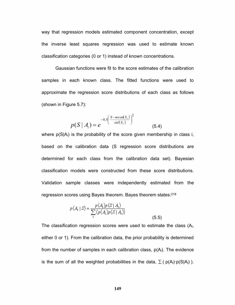
149
way that regression models estimated component concentration, except
the inverse least squares regression was used to estimate known
classification categories (0 or 1) instead of known concentrations.
Gaussian functions were fit to the score estimates of the calibration
samples in each known class. The fitted functions were used to
approximate the regression score distributions of each class as follows
(shown in Figure 5.7):
2
5.0
)|(
i
i
Sstd
SmeanS
i eASp (5.4)
where p(S|Ai) is the probability of the score given membership in class i,
based on the calibration data (S regression score distributions are
determined for each class from the calibration data set). Bayesian
classification models were constructed from these score distributions.
Validation sample classes were independently estimated from the
regression scores using Bayes theorem. Bayes theorem states:218
(5.5)
The classification regression scores were used to estimate the class (Ai,
either 0 or 1). From the calibration data, the prior probability is determined
from the number of samples in each calibration class, p(Ai). The evidence
is the sum of all the weighted probabilities in the data, ∑ ( p(Ai)·p(S|Ai) ).
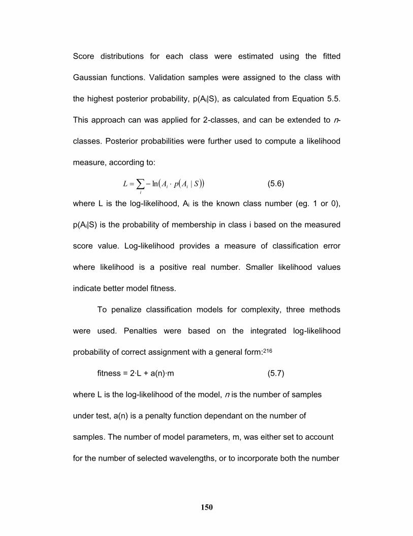
150
Score distributions for each class were estimated using the fitted
Gaussian functions. Validation samples were assigned to the class with
the highest posterior probability, p(Ai|S), as calculated from Equation 5.5.
This approach can was applied for 2-classes, and can be extended to n-
classes. Posterior probabilities were further used to compute a likelihood
measure, according to:
i
ii SApAL |ln (5.6)
where L is the log-likelihood, Ai is the known class number (eg. 1 or 0),
p(Ai|S) is the probability of membership in class i based on the measured
score value. Log-likelihood provides a measure of classification error
where likelihood is a positive real number. Smaller likelihood values
indicate better model fitness.
To penalize classification models for complexity, three methods
were used. Penalties were based on the integrated log-likelihood
probability of correct assignment with a general form:216
fitness = 2·L + a(n)·m (5.7)
where L is the log-likelihood of the model, n is the number of samples
under test, a(n) is a penalty function dependant on the number of
samples. The number of model parameters, m, was either set to account
for the number of selected wavelengths, or to incorporate both the number
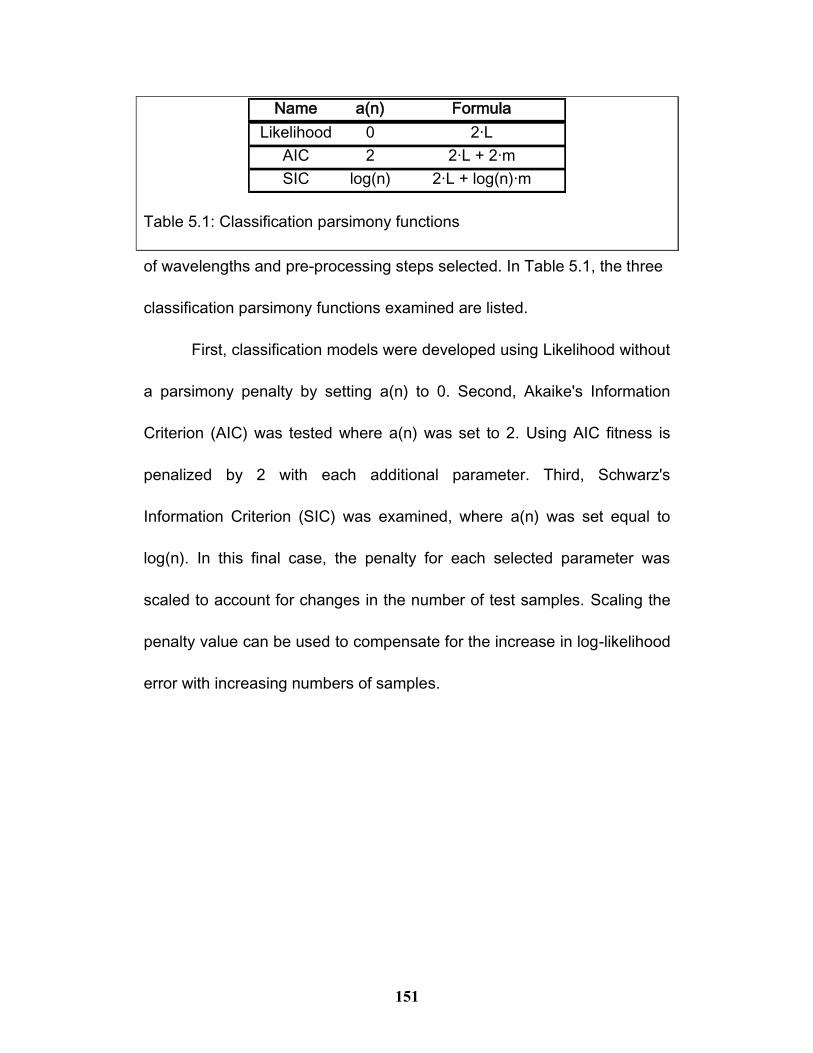
151
of wavelengths and pre-processing steps selected. In Table 5.1, the three
classification parsimony functions examined are listed.
First, classification models were developed using Likelihood without
a parsimony penalty by setting a(n) to 0. Second, Akaike's Information
Criterion (AIC) was tested where a(n) was set to 2. Using AIC fitness is
penalized by 2 with each additional parameter. Third, Schwarz's
Information Criterion (SIC) was examined, where a(n) was set equal to
log(n). In this final case, the penalty for each selected parameter was
scaled to account for changes in the number of test samples. Scaling the
penalty value can be used to compensate for the increase in log-likelihood
error with increasing numbers of samples.
Name a(n) Formula
Likelihood 0 2·L
AIC 2 2·L + 2·m
SIC log(n) 2·L + log(n)·m
Table 5.1: Classification parsimony functions
152
5.6.6 Selection of Models
As a quasi-random search process, no single execution of a
genetic algorithm is guaranteed to select the best possible model. Instead
the genetic algorithm was run several times, and best results for each
model size were selected from the aggregated results. To allow direct
comparisons, parsimony-free fitness values were calculated and stored in
addition to the parsimony-penalized fitness. Statistical methods were
applied to select a model for each number of pre-processing steps. Least
complex models showing statistically significant improvement over all
simpler models were selected. Statistical comparisons for regression
models were based on the f-test to compare between MSE values, while
classification models were compared using the chi-squared test to
evaluate differences between log-likelihood values. Best fit models for
each pre-processing scheme were then compared. Among the several
models selected for comparison, some use many more or many fewer
regression parameters than required and can be rejected. A final
processing model is selected from the remaining models based on results
of the validation data. Remaining models should also be examined
graphically, to ensure that selected wavelengths map to spectral features,
and to ensure that cross-validation iterations show consistent results.
153
Examples of graphical results are shown in Figures 5.3, 5.4, 5.6, 5.7, and
5.8. Figures 5.3 and 5.6 both show the selected regression parameters
and calibration weightings along with the pre-processed spectra. Because
of shift and transformation in the spectral axis as a result of the various
pre-processing options, selected wavelengths may not correspond
perfectly to expected spectral features. However, selected wavelengths
must correspond to portions of the pre-processed spectrum that contain
information about the property under study. Some selected features may
represent background offset corrections, and others should map to
regions with spectral features. Calibration coefficients weighted
inconsistently between cross-validation steps indicate that a model is too
large, and may be adapted to noise rather than analyte signal. Figure 5.4
shows results from the optimal processing model for estimating blood
lactate content from in vivo NIR spectra measured through the fingernail.
Figure 5.7 shows the distributions of classes in the calibration and the
associated Gaussian probability distributions. Figure 5.8 shows results
from the optimal model for assignment of starch class membership from
infrared spectra. Models displaying inconsistency were rejected.
154
5.7 Test Data
Two sets of data were examined to test the use of the regression
and classification genetic algorithm.
5.7.1 Regression Data Set
Near-infrared reflectance spectra for in-vivo measurement of lactate
were examined.95 Spectra were recorded from 1000 to 2500 nm with a
16 cm-1 resolution, using an FT-NIR spectrometer to sample light diffusely
reflected from the fingernails of ten adult subjects.95 Spectra and reference
blood samples were acquired at four intervals before, during and after a
30-second sprint on a modified isokinetic cycle. Reference blood lactate
concentrations were measured from the reference blood samples. From
partial least squares regression analysis, using the region of the spectrum
from 1500 to 1750 nm, lactate concentration was determined with a
standard error of cross validation of 2.21 mmol•l-1 and a correlation
coefficient of 0.74.
155
5.7.2 Classification Data Set
Mid-infrared spectral data for classification of starches were
provided by Dr. Pierre Dardenne and Dr. Juan Antonio Fernández Pierna
from the Walloon Agricultural Research Centre in Gembloux (Belgium).217,
221 Spectra from 215 starch samples were recorded from 4000 to 600 cm-1
at a 3.51 cm-1 (967 points) resolution using a FTIR spectrometer equipped
with an ATR probe. This data was the subject of the 'Chimiometrie 2005'
contest. Starches were grouped into 2 classes, with 107 and 108
members in each respective class. As a result, the two classification
groups were approximately equal in size.

156
5.8 Results and Discussion
Multiple linear regression and Bayesian classification models were
selected for processing two datasets using the genetic algorithm
5 10 15 20 25
1
3
5
5 10 15 20 25
1
3
5
5 10 15 20 25
1
3
5
1
1.2
1.4
1.6
1.8
2
(a)
(b)
(c)
Co
un
t o
f P
rep
rocessin
g S
tep
s
Regression Model Size
Re
gre
ssio
n M
od
el E
rror
5 10 15 20 25
1
3
5
5 10 15 20 25
1
3
5
5 10 15 20 25
1
3
5
1
1.2
1.4
1.6
1.8
2
1
1.2
1.4
1.6
1.8
2
(a)
(b)
(c)
Co
un
t o
f P
rep
rocessin
g S
tep
s
Regression Model Size
Re
gre
ssio
n M
od
el E
rror
Figure 5.2: Models for determining lactate concentration from NIR spectra
were selected by a genetic algorithm. Results are presented as model
error (grayscale intensity) for each model size and complexity (position).
Dark regions indicate low model error, or good models. Bright regions
show high model error and indicate poor models. In the Figures
optimization results are shown: (a) without parsimony, (b) using parsimony
for the number of wavelengths selected, and (c) using parsimony for both
the number wavelengths and pre-processing steps selected.
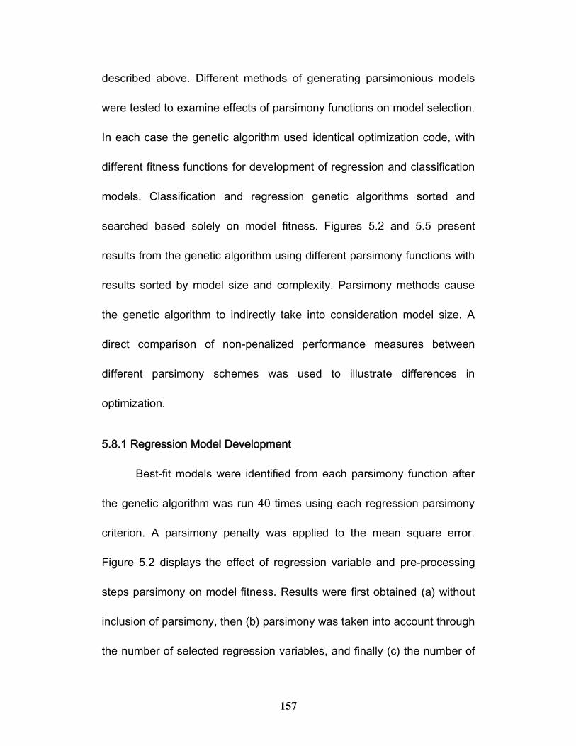
157
described above. Different methods of generating parsimonious models
were tested to examine effects of parsimony functions on model selection.
In each case the genetic algorithm used identical optimization code, with
different fitness functions for development of regression and classification
models. Classification and regression genetic algorithms sorted and
searched based solely on model fitness. Figures 5.2 and 5.5 present
results from the genetic algorithm using different parsimony functions with
results sorted by model size and complexity. Parsimony methods cause
the genetic algorithm to indirectly take into consideration model size. A
direct comparison of non-penalized performance measures between
different parsimony schemes was used to illustrate differences in
optimization.
5.8.1 Regression Model Development
Best-fit models were identified from each parsimony function after
the genetic algorithm was run 40 times using each regression parsimony
criterion. A parsimony penalty was applied to the mean square error.
Figure 5.2 displays the effect of regression variable and pre-processing
steps parsimony on model fitness. Results were first obtained (a) without
inclusion of parsimony, then (b) parsimony was taken into account through
the number of selected regression variables, and finally (c) the number of
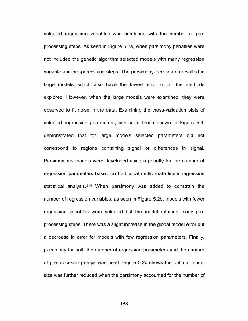
158
selected regression variables was combined with the number of pre-
processing steps. As seen in Figure 5.2a, when parsimony penalties were
not included the genetic algorithm selected models with many regression
variable and pre-processing steps. The parsimony-free search resulted in
large models, which also have the lowest error of all the methods
explored. However, when the large models were examined, they were
observed to fit noise in the data. Examining the cross-validation plots of
selected regression parameters, similar to those shown in Figure 5.4,
demonstrated that for large models selected parameters did not
correspond to regions containing signal or differences in signal.
Parsimonious models were developed using a penalty for the number of
regression parameters based on traditional multivariate linear regression
statistical analysis.214 When parsimony was added to constrain the
number of regression variables, as seen in Figure 5.2b, models with fewer
regression variables were selected but the model retained many pre-
processing steps. There was a slight increase in the global model error but
a decrease in error for models with few regression parameters. Finally,
parsimony for both the number of regression parameters and the number
of pre-processing steps was used. Figure 5.2c shows the optimal model
size was further reduced when the parsimony accounted for the number of
159
both regression variables and pre-processing steps. In this final case,
models with fewer pre-processing steps were preferentially explored by
the genetic algorithm because of the parsimony penalties. Larger models
were also examined; however, parsimony penalties emphasized the
development of small models. Use of both parsimony criteria constrained
the algorithm to small models. As a result, the genetic algorithm did not
search for solutions with large numbers of regression variables and pre-
processing steps. Large models selected when using both parsimony
criteria had higher error than models of corresponding size selected in the
parsimony-free algorithm. In contrast, small models selected when using
both parsimony criteria had lower error than models of corresponding size
selected in the parsimony-free algorithm. The large models selected
without parsimony had the lowest total error of all the models developed.
However, these models were unnecessarily complicated. One potential
disadvantage of using parsimony is a decrease in the selection of complex
models with low error. This can be a problem because complex models
can serve as intermediate steps in the evolution of simple models.
Nonetheless, the most efficient model with fewest pre-processing steps,
regression parameters, and lowest error was located using the parsimony
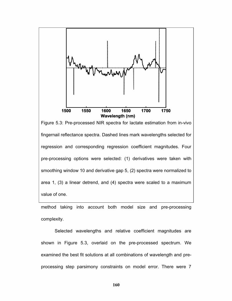
160
method taking into account both model size and pre-processing
complexity.
Selected wavelengths and relative coefficient magnitudes are
shown in Figure 5.3, overlaid on the pre-processed spectrum. We
examined the best fit solutions at all combinations of wavelength and pre-
processing step parsimony constraints on model error. There were 7
1500 1550 1600 1650 1700 1750
Wavelength (nm)
1500 1550 1600 1650 1700 1750
Wavelength (nm)
Figure 5.3: Pre-processed NIR spectra for lactate estimation from in-vivo
fingernail reflectance spectra. Dashed lines mark wavelengths selected for
regression and corresponding regression coefficient magnitudes. Four
pre-processing options were selected: (1) derivatives were taken with
smoothing window 10 and derivative gap 5, (2) spectra were normalized to
area 1, (3) a linear detrend, and (4) spectra were scaled to a maximum
value of one.
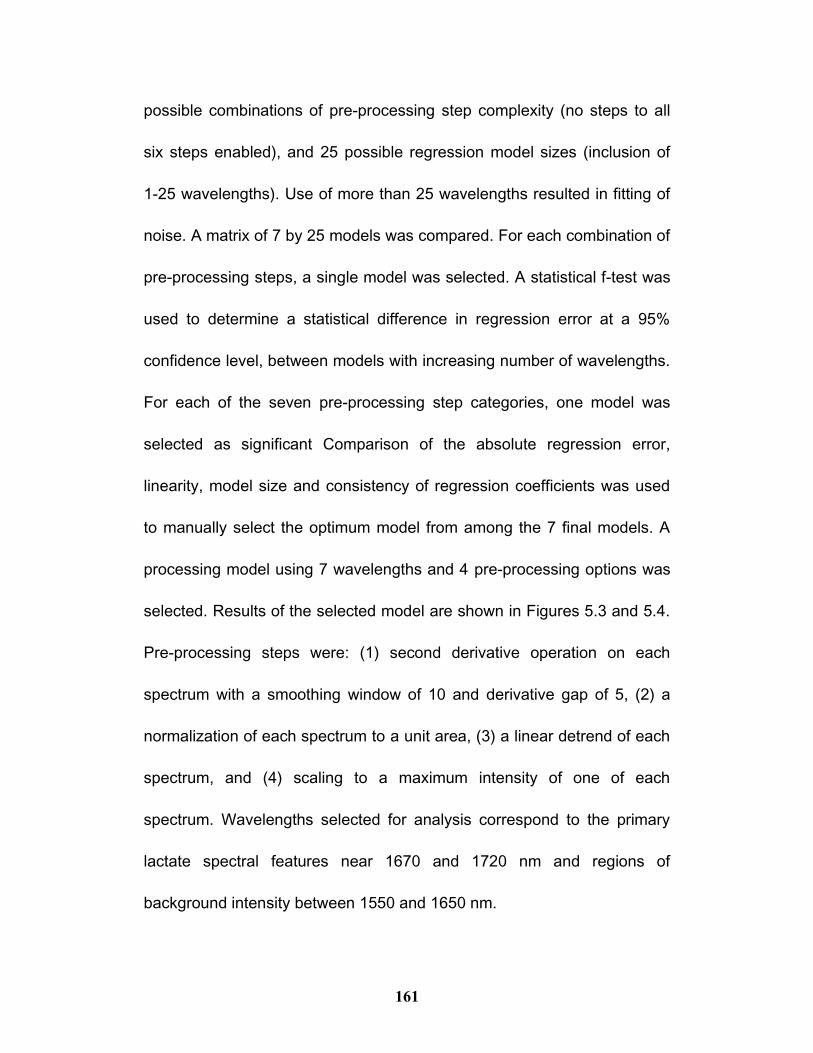
161
possible combinations of pre-processing step complexity (no steps to all
six steps enabled), and 25 possible regression model sizes (inclusion of
1-25 wavelengths). Use of more than 25 wavelengths resulted in fitting of
noise. A matrix of 7 by 25 models was compared. For each combination of
pre-processing steps, a single model was selected. A statistical f-test was
used to determine a statistical difference in regression error at a 95%
confidence level, between models with increasing number of wavelengths.
For each of the seven pre-processing step categories, one model was
selected as significant Comparison of the absolute regression error,
linearity, model size and consistency of regression coefficients was used
to manually select the optimum model from among the 7 final models. A
processing model using 7 wavelengths and 4 pre-processing options was
selected. Results of the selected model are shown in Figures 5.3 and 5.4.
Pre-processing steps were: (1) second derivative operation on each
spectrum with a smoothing window of 10 and derivative gap of 5, (2) a
normalization of each spectrum to a unit area, (3) a linear detrend of each
spectrum, and (4) scaling to a maximum intensity of one of each
spectrum. Wavelengths selected for analysis correspond to the primary
lactate spectral features near 1670 and 1720 nm and regions of
background intensity between 1550 and 1650 nm.

162
Results using the linear calibration model selected by the genetic
algorithm for estimation of lactate concentration are shown in Figure 5.4.
Lafrance showed a 5-component partial least squares model to best
estimate lactate concentration.95 In comparison, the model selected by the
genetic algorithm performed better, the standard error of cross validation
decreased and coefficient of regression increased. Standard error
decreased from 2.21 to 1.76 mmol · l-1 and the correlation coefficient
SECV = 1.76
r = 0.83
0 2 4 6 8 10 12
0
2
4
6
8
10
12
Reference Lactate Concentration (mmol/l)
Esti
mate
d L
ac
tate
Co
ncen
trati
on
(m
mo
l/l)
SECV = 1.76
r = 0.83
0 2 4 6 8 10 12
0
2
4
6
8
10
12
Reference Lactate Concentration (mmol/l)
Esti
mate
d L
ac
tate
Co
ncen
trati
on
(m
mo
l/l)
Figure 5.4: Lactate was estimated for 10 subjects using in-vivo NIR
spectra versus a reference measure of lactate. Cross-validation using a 7-
component multilinear regression model was used to estimate the lactate
concentrations from spectral data between 1500 and 1750 nm; n = 40,
r = 0.83, SECV = 1.76 mmol•l-1. Regression estimates were determined
from data at 1519, 1604, 1645, 1669, 1724, 1733 and 1734 nm.
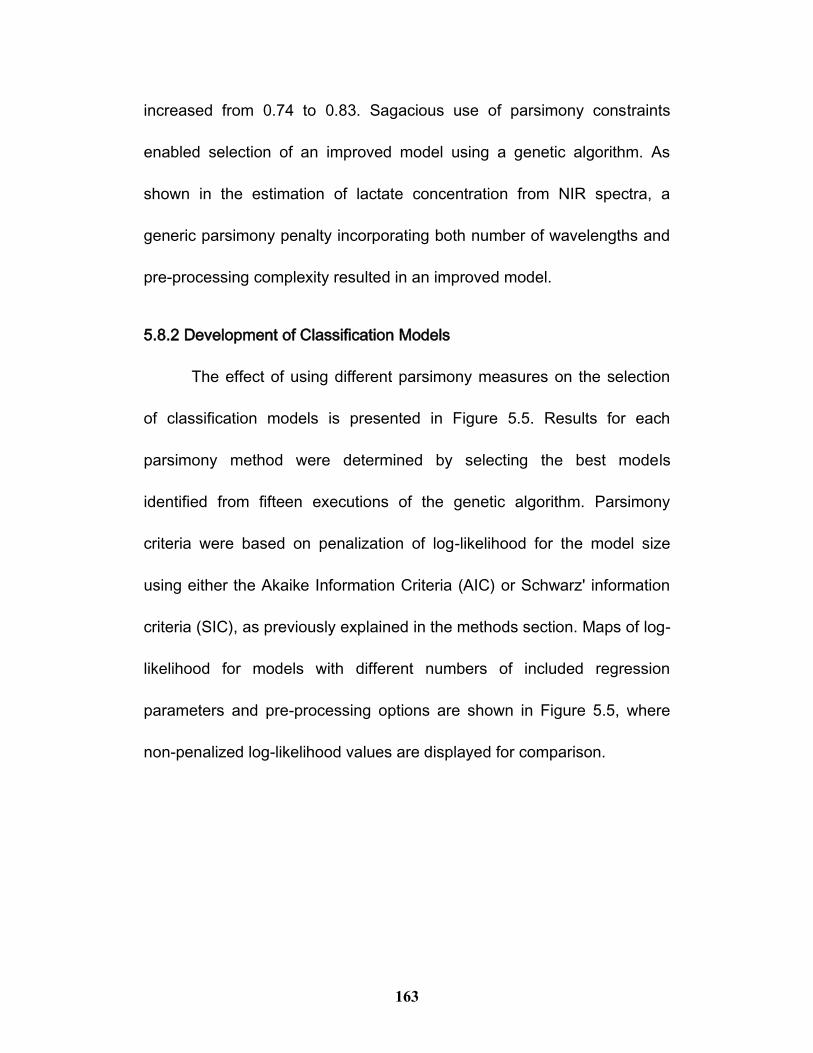
163
increased from 0.74 to 0.83. Sagacious use of parsimony constraints
enabled selection of an improved model using a genetic algorithm. As
shown in the estimation of lactate concentration from NIR spectra, a
generic parsimony penalty incorporating both number of wavelengths and
pre-processing complexity resulted in an improved model.
5.8.2 Development of Classification Models
The effect of using different parsimony measures on the selection
of classification models is presented in Figure 5.5. Results for each
parsimony method were determined by selecting the best models
identified from fifteen executions of the genetic algorithm. Parsimony
criteria were based on penalization of log-likelihood for the model size
using either the Akaike Information Criteria (AIC) or Schwarz' information
criteria (SIC), as previously explained in the methods section. Maps of log-
likelihood for models with different numbers of included regression
parameters and pre-processing options are shown in Figure 5.5, where
non-penalized log-likelihood values are displayed for comparison.
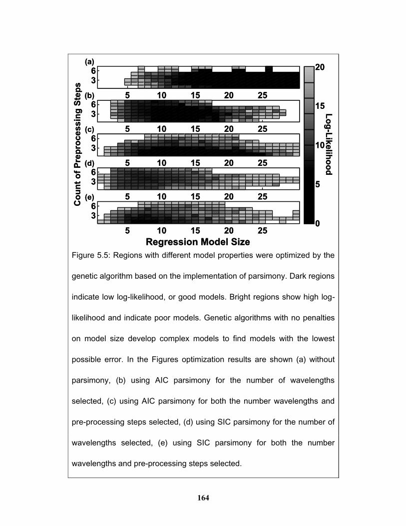
164
Co
un
t o
f P
rep
rocessin
g S
tep
s
Regression Model Size
5 10 15 20 25
36
5 10 15 20 25
36
5 10 15 20 25
36
5 10 15 20 25
36
5 10 15 20 25
36
0
5
10
15
20
Lo
g-L
ikelih
oo
d
(a)
(b)
(c)
(d)
(e)
Co
un
t o
f P
rep
rocessin
g S
tep
s
Regression Model Size
5 10 15 20 25
36
5 10 15 20 25
36
5 10 15 20 25
36
5 10 15 20 25
36
5 10 15 20 25
36
0
5
10
15
20
Lo
g-L
ikelih
oo
d
(a)
(b)
(c)
(d)
(e)
Figure 5.5: Regions with different model properties were optimized by the
genetic algorithm based on the implementation of parsimony. Dark regions
indicate low log-likelihood, or good models. Bright regions show high log-
likelihood and indicate poor models. Genetic algorithms with no penalties
on model size develop complex models to find models with the lowest
possible error. In the Figures optimization results are shown (a) without
parsimony, (b) using AIC parsimony for the number of wavelengths
selected, (c) using AIC parsimony for both the number wavelengths and
pre-processing steps selected, (d) using SIC parsimony for the number of
wavelengths selected, (e) using SIC parsimony for both the number
wavelengths and pre-processing steps selected.
165
1000150020002500300035000
0.2
0.4
0.6
0.8
1
Wavenumber (cm-1)
Pre
pro
ces
sed
Sp
ectr
al
Inte
ns
ity
(arb
itra
ry u
nit
s)
1000150020002500300035000
0.2
0.4
0.6
0.8
1
Wavenumber (cm-1)
Pre
pro
ces
sed
Sp
ectr
al
Inte
ns
ity
(arb
itra
ry u
nit
s)
Figure 5.6: Pre-processed starch spectral data, with the normalized
regression coefficients shown as dashed lines to indicate the portions of
the spectrum selected for analysis. No pre-processing options were
selected in the optimal model. Data at 1133, 1329, 1352, 1369 and
2185 cm-1 were selected for developing the classification score.
166
Similar to the comparisons for the regression model penalties,
classification models were initially developed without penalization for
model size (as measured by the number of wavelengths) and complexity
(as measured by the number of pre-processing steps). Classification
models were also developed using AIC to penalize fitness based on only
the model size or a combination of the model size and complexity, as
shown in Figures 5.5b and 5.5c respectively. Finally, classification models
were developed using SIC, using either the model size or a combination of
the model size and complexity, as shown in Figures 5.5d and 5.5e.
Schwartz's information criterion uses a penalty scaled by the
number of samples used for testing the model. This penalty biased the
search towards the selection of small models and prevented models with
moderate complexity from being fully exploited. Using the Akaike
information criteria small models were emphasized over very large
models, while still exploring intermediate models. In the fitness maps in
Figure 5.5, shifts in model exploration result in shifts in the dark basin
representing the best models located. Without parsimony, large complex
models are selected. When parsimony measures based on model size are
included in the genetic algorithm, optimal models requiring fewer
wavelengths are found. When constrained with both model size and
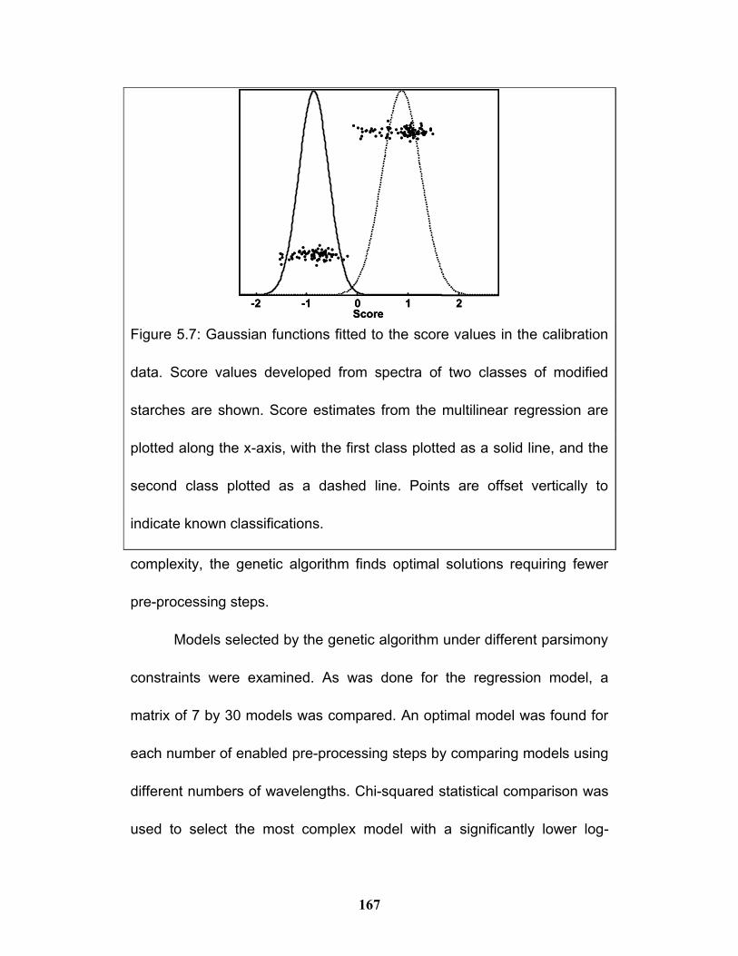
167
complexity, the genetic algorithm finds optimal solutions requiring fewer
pre-processing steps.
Models selected by the genetic algorithm under different parsimony
constraints were examined. As was done for the regression model, a
matrix of 7 by 30 models was compared. An optimal model was found for
each number of enabled pre-processing steps by comparing models using
different numbers of wavelengths. Chi-squared statistical comparison was
used to select the most complex model with a significantly lower log-
-2 -1 0 1 2Score
-2 -1 0 1 2Score
Figure 5.7: Gaussian functions fitted to the score values in the calibration
data. Score values developed from spectra of two classes of modified
starches are shown. Score estimates from the multilinear regression are
plotted along the x-axis, with the first class plotted as a solid line, and the
second class plotted as a dashed line. Points are offset vertically to
indicate known classifications.
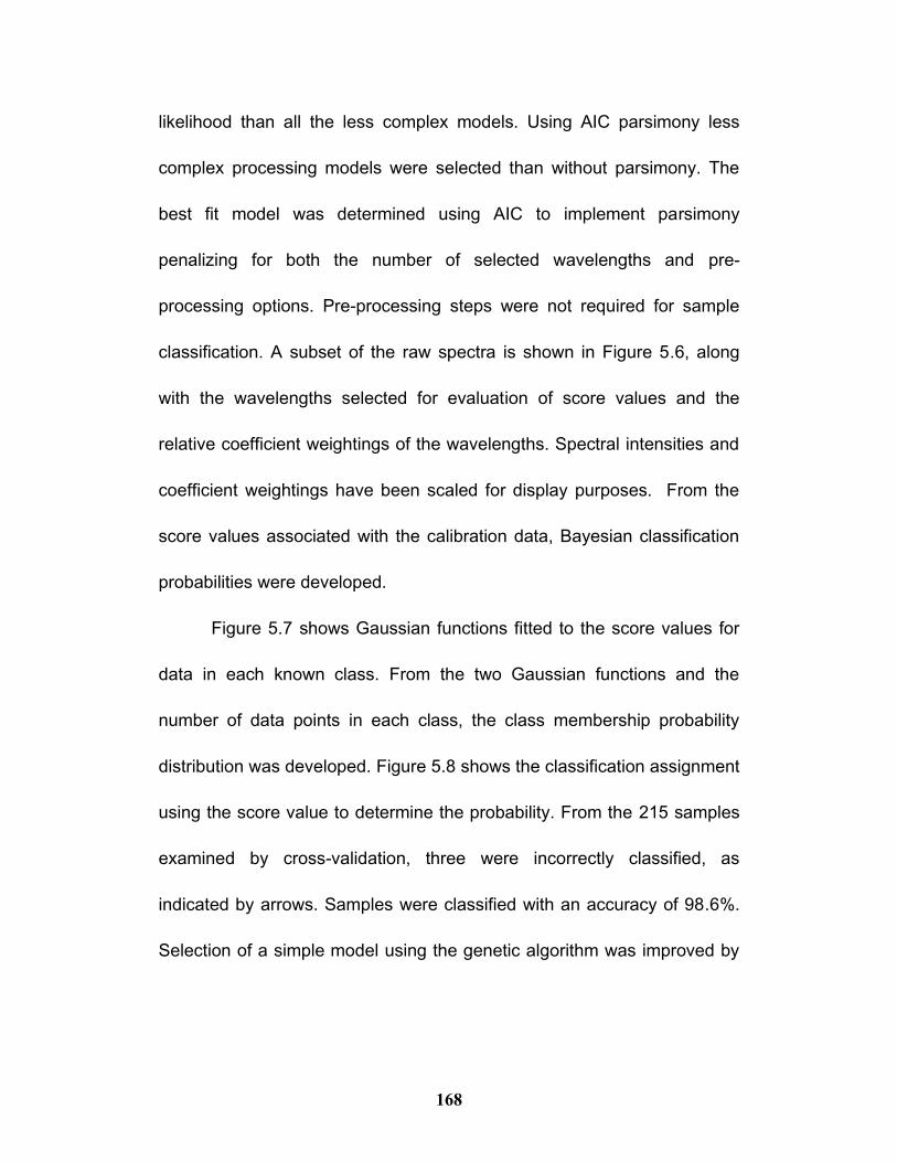
168
likelihood than all the less complex models. Using AIC parsimony less
complex processing models were selected than without parsimony. The
best fit model was determined using AIC to implement parsimony
penalizing for both the number of selected wavelengths and pre-
processing options. Pre-processing steps were not required for sample
classification. A subset of the raw spectra is shown in Figure 5.6, along
with the wavelengths selected for evaluation of score values and the
relative coefficient weightings of the wavelengths. Spectral intensities and
coefficient weightings have been scaled for display purposes. From the
score values associated with the calibration data, Bayesian classification
probabilities were developed.
Figure 5.7 shows Gaussian functions fitted to the score values for
data in each known class. From the two Gaussian functions and the
number of data points in each class, the class membership probability
distribution was developed. Figure 5.8 shows the classification assignment
using the score value to determine the probability. From the 215 samples
examined by cross-validation, three were incorrectly classified, as
indicated by arrows. Samples were classified with an accuracy of 98.6%.
Selection of a simple model using the genetic algorithm was improved by
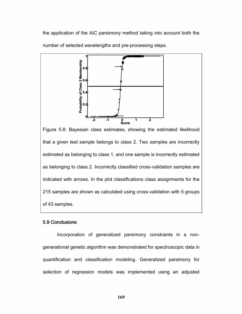
169
the application of the AIC parsimony method taking into account both the
number of selected wavelengths and pre-processing steps.
5.9 Conclusions
Incorporation of generalized parsimony constraints in a non-
generational genetic algorithm was demonstrated for spectroscopic data in
quantification and classification modeling. Generalized parsimony for
selection of regression models was implemented using an adjusted
-2 -1 0 1 20
0.2
0.4
0.6
0.8
1
Score
Pro
ba
bil
ity o
f C
lass
2 M
em
be
rsh
ip
-2 -1 0 1 20
0.2
0.4
0.6
0.8
1
Score
Pro
ba
bil
ity o
f C
lass
2 M
em
be
rsh
ip
Figure 5.8: Bayesian class estimates, showing the estimated likelihood
that a given test sample belongs to class 2. Two samples are incorrectly
estimated as belonging to class 1, and one sample is incorrectly estimated
as belonging to class 2. Incorrectly classified cross-validation samples are
indicated with arrows. In the plot classifications class assignments for the
215 samples are shown as calculated using cross-validation with 5 groups
of 43 samples.
170
RMSE, while parsimony for selection of classification models was
implemented using penalized log-likelihood. Model size was measured by
the number of wavelengths, and model complexity was measured by the
number of pre-processing steps. When unconstrained, the genetic
algorithm was shown to search for large, complex models. Single
parsimony using only the number of wavelengths was effective in directing
the search algorithm towards exploration of smaller models. Likewise, dual
parsimony using both the number of wavelengths and pre-processing
steps resulted in optimization of models with fewer wavelengths and also
fewer pre-processing steps. The constrained algorithm returned solutions
with slightly more error, but successfully located smaller models not
identified without parsimony constraints. The quality of small models is
very important for practical reasons, while much larger models are less
useful. Other than as intermediate solutions, very complex models will not
likely find practical application. We found that dataset independent
parsimony functions affected these two data sets in a similar manner,
resulting in the selection of simple processing models.
5.10 Acknowledgements
Funding for this research was provided by the National Science and
Engineering Research Council of Canada (NSERC). The authors thank

171
Dr. Pierre Dardenne and Dr. Juan Antonio Fernández Pierna from the
Walloon Agricultural Research Centre in Gembloux (Belgium) for providing
the starch data,217 and Dr. Royston Goodacre of the Institute of Biological
Sciences, University of Wales, Aberystwyth for additional data used in
testing the algorithm.212 Finally, the authors would also like to thank Karen
Esmonde-White for editorial comments.
172
Chapter 6. Estimation of Myoglobin Oxygen
Saturation from Spectra of Cardiac Tissue using
Multivariate Curve Resolution
Improvements to spectroscopic quantification in turbid media have
been demonstrated using novel instrumentation and data processing
methods. In the previous chapter, a novel method for applying parsimony
in the selection of processing models using a genetic algorithm was
demonstrated. In particular, a regression-based data processing model
was identified with a 41% reduction in regression error as compared to the
best user-developed model. Genetic algorithm based development of data
processing models are most useful where calibration conditions are
consistent with validation and usage conditions.
In systems where the chemical environment is expected to vary
from the initial calibration conditions, self-adapting methods can be used
to compensate for changes. Multivariate curve resolution techniques are
one such example of self-adapting methods. In multivariate curve
resolution the measured data is used to directly estimate the signal
response and sample composition.
173
In this chapter a method for adaptively modelling tissue spectra is
presented. Spectral features in biological systems are not identical to
spectral features of the isolated components. Reasons for this include the
pH of the chemical environment, the multitude of interactions, and the
spectral transformations caused by light scattering. To improve
quantification in biological systems, multivariate curve resolution can
recover the analyte concentrations and pure component spectral profiles.
In this chapter we describe a novel application of multivariate curve
resolution for estimating myoglobin oxygen saturation in cardiac tissue.
Matlab code for the MCR routine described here is provided in appendix
D. A brief introduction to multivariate curve resolution is presented prior to
the main manuscript.
6.1 Multivariate Curve Resolution
Multivariate curve resolution (MCR) refers to a family of data
processing techniques used for simultaneous determination of
concentrations and pure spectra of mixtures based on perturbations in the
data.223 One member of the MCR family is alternating least-squares
multivariate curve resolution (MCR-ALS), based on an alternating series of
least squares concentration and spectral profile estimates.224 Central to
the alternating least squares algorithm are constraints for bounding
174
solutions within physically relevant limits. Constraints are used to
mathematically resolve the chemical components.225, 226 MCR algorithms
typically use constraints such as closure, non-negativity, selectivity,
normalization, and equality.227, 228 Selections and implementations of
constraints are the primary differences between MCR-ALS algorithms.224
Spectral data is normally assumed to be non-negative, as are chemical
concentrations. However, in tissue spectroscopy second derivatives are
commonly taken as a data pre-treatment step. When derivatives are
taken, spectral intensities can assume negative values. Non-negativity
cannot be used as a constraint when processing derivative spectra.
Likewise concentration closure is no longer applicable when spectral
backgrounds are subtracted because some spectral contribution from
each species may be lost. Pre-processing steps must be carefully
selected to ensure that constraints chosen for the MCR remain applicable.
An initial starting point must be supplied to MCR algorithms. The
similarity of the starting guess to the true component is important, and
influences the results of the MCR algorithm. Suitable starting points can
include principal component spectra as derived from singular value
decompositions, or better yet, measured spectra of the isolated
components. In addition to estimated spectra, the total number of
175
components present in the mixture must be supplied to the MCR
algorithm. Methods suggested in the literature include use of prediction
error sum of squares plots (scree plots) examining the residual error from
fitting varying numbers of principal components to the experimental data.
MCR algorithms use systematic variations in the data to isolate signal
contributions from different species, and so data should include
independent variations between components. If components have spectra
or concentration profiles that are too similar, a lack of selectivity can lead
to significant ambiguity in the MCR solutions.229
Multivariate curve resolution techniques allow for the determination
of both the concentrations and the spectral profiles for each component in
a mixture, given a suitable starting point. By allowing an MCR routine to
determine the optimal spectra directly from measured data, pure
component spectra are estimated for the relevant chemical environment.
Absolute chemical concentrations are not determined from the MCR
algorithm because of scaling constraints. Instead, relative composition is
determined and can be related to absolute concentration using known
system properties.
176
6.2 Manuscript
Estimation of Myoglobin Oxygen Saturation from Spectra of Cardiac
Tissue using Multivariate Curve Resolution
Authors:
Francis W.L. Esmonde-White, Lorilee S.L. Arakaki,
Kenneth A. Schenkman, Wayne A. Ciesielski, David H. Burns
6.3 Abstract
A method for adaptive modeling of spectra from tissue for
myoglobin oxygen saturation was developed. The multivariate curve
resolution (MCR) technique was compared with a classical least squares
method for estimation of myoglobin oxygen saturation in simulated and
biological cardiac tissue. Tissue simulations with fixed and variable
hemoglobin concentrations were examined to compare the performance of
the techniques under different conditions. Myoglobin saturation estimates
using MCR with variable hemoglobin composition were shown to decrease
estimation error by 75% compared to least squares estimates. The range
of myoglobin saturation required for MCR to function was examined.
Results show that the spectral data set must include myoglobin saturation
values that vary from at least 85% to 100% for myoglobin oxygen
saturation calibration using MCR. Myoglobin oxygen saturation endpoints
177
in 9 guinea pig hearts were estimated from spectra using MCR and
classical least squares. Results showed saturation estimates using MCR
to be better than estimates using classical least squares. Endpoints at the
100% level were estimated to be 89 +/- 4% using MCR as compared to
199 +/- 54 % using classical least squares. MCR provides a means for
practical measurements in clinical settings.
6.4 Keywords
Multivariate curve resolution, MCR, self-modeling curve resolution,
SMCR, myoglobin oxygen saturation
6.5 Introduction
Visible and near-infrared spectroscopic measurements in living
tissue are routinely used to measure blood oxygenation.128-130 Pulse
oximetry uses distinctions between the absorption spectra of
deoxyhemoglobin (Hb) and oxyhemoglobin (HbO2) to rapidly measure
blood oxygen saturation. Spectroscopic difference measurements
between the systolic and diastolic moments, while the heart is beating and
at rest, enable a hemoglobin-selective oxygen saturation measurement.
However, pulse oximetry measurements cannot be used to measure
oxygen saturation within cells, where oxygen is ultimately consumed.

178
Myoglobin is present in skeletal muscle and the heart.
Measurement of myoglobin oxygen saturation in cardiac tissue has the
potential to provide information about intracellular oxygenation during
surgical procedures. Standard imaging modalities, such as magnetic
resonance imaging, that are widely used to measure oxygen content in
blood or tissue may not be compatible with the small spaces in a surgical
suite or may not adequately discriminate tissue from blood. Visible-near-
infrared (VIS-NIR) spectroscopy is currently explored as a measurement
of myoglobin oxygen saturation. Spectroscopic systems are relatively
small and resulting spectra can be used to quantify oxygen content in
blood, tissue or both. The high spatial resolution and specificity of VIS-NIR
spectra can be used to distinguish normal arterial perfusion from regional
ischemia and show areas of low, medium, and high deoxygenation during
reperfusion of cardiac tissue.88
Spectroscopic methods for measuring hemoglobin oxygen
saturation noninvasively have widely been reported.125, 134, 230 Hemoglobin
oxygen saturation in arterial blood can be measured by taking the spectral
difference between points of maximum and minimum blood volume during
the cardiac pulse to isolate the spectral contribution of red blood cells from
surrounding tissue. However, the same method cannot be applied to
179
spectral measurements of myoglobin oxygen saturation in cardiac and
skeletal muscle because myoglobin concentration does not change rapidly
within muscle cells. The similarity of myoglobin and hemoglobin NIR
spectra further complicates measurements of myoglobin oxygen
saturation (SMb). More complex processing methods than used in pulse
oximetry are utilized for determination of relative deoxymyoglobin (Mb)
and oxymyoglobin (MbO2) concentrations. Myoglobin oxygen saturation
within tissue can be calculated from the relative deoxymyoglobin and
oxymyoglobin concentrations, indicating the intracellular oxygen partial
pressure.
Methods have been reported for spectroscopic measurement of SMb
in the presence of hemoglobin in vitro both without scattering,120 and also
in the presence of scattering.153, 231 In addition to in vitro studies,
myoglobin oxygen saturation has been measured spectroscopically under
ex vivo and in vivo conditions by perfusing tissue with a buffer solution to
remove hemoglobin interference.101, 232, 233 Calibration spectra are required
with classical least squares (CLS) and partial least squares (PLS) to
determine SMb for samples at intermediate oxygen saturations.
Unfortunately, calibration spectra cannot be measured in tissue. Instead,
in vitro calibrations developed with PLS can be transferred and used for ex
180
vivo and in vivo measurements with scattering and hemoglobin
interference.97, 234 Using PLS, calibrations require spectra to be collected
at 0% and 100% O2 saturation for scaling the data to account for
differences between samples.97 Physical manipulations such as occlusion
of blood flow to tissue and manipulations of the inspired air oxygen
content have been performed to reach 0% and 100% O2 saturations.
Manipulations for calibration such as these are impractical for
measurements in a surgical setting because myoglobin oxygen saturation
should not reach the limit values under normal physiological conditions.
Spectroscopic measurement of SMb is further complicated because
spectra of individual components are imperfectly known, because
reference SMb calibration values are not available, and because light
scattering causes nonlinear transformations between spectra measured
with and without scattering.235 Reference spectra are measured from
purified samples and can include a scatterer. Differences in scattering
between spectra of reference and test samples lead to fitting errors in the
data processing. Light scattering varies between individuals, and over time
also varies within each individual.236 Because of these variations,
scattering is problematic even when calibrations are obtained directly from
181
tissue. Spectra for each individual subject may be acquired over short time
periods to minimize temporal variations in light scattering.
Multivariate curve resolution (MCR) is used to isolate pure
component spectra and pure component compositions from a series of
spectra.237, 238 MCR allows scattering-transformed spectra to be estimated
directly from ex vivo or in vivo tissue spectra. Estimation of component
concentrations using scattering-transformed spectra, instead of using
reference spectra measured in vitro as in CLS and PLS, should improve
least squares estimates of component concentrations. MCR has been
demonstrated to mathematically isolate pure component spectra from
mixtures of multiple components with varying sample composition in
recorded spectral data.223, 239, 240 Components are isolated by MCR using
constraints such as closure, non-negativity and normalization to limit the
range of valid solutions.239, 241 MCR is particularly useful in systems where
physical limitations prohibit measurement of isolated pure component
spectra. Examples include species present in equilibria which can never
be completely isolated and living tissue where reference spectra may be
inaccurate if recorded outside the scattering environment.237, 238, 242
In this paper, we report the application of MCR to measurement of
myoglobin oxygen saturation using VIS-NIR spectra of cardiac tissue
182
perfused with red blood cells. Pure spectra and relative concentrations of
Mb and MbO2 were estimated by the MCR algorithm, using in vitro spectra
of myoglobin and hemoglobin measured at 0 % and 100 % oxygen
saturations for initial estimates of pure component spectra. Estimated
myoglobin concentrations were then used to calculate SMb. Analysis using
the MCR method was compared to a classical least-squares (CLS)
analysis method by examining simulated tissue spectral data and spectra
acquired from cardiac tissue. Simulated tissue data were also used to
examine effects of the sampled oxygen saturation span on MCR analysis
accuracy.
6.6 Theory
Multivariate curve resolution refers to a family of data processing
techniques used for simultaneous determination of concentrations and
pure spectra of mixtures based on perturbations in the data.223 One
member of the MCR family is alternating least-squares multivariate curve
resolution (MCR-ALS), based on a series of alternating least squares
estimates of composition and spectral components.224 Constraints are
used to mathematically isolate the chemical components by providing
boundaries to limit the possible solutions.225, 226 Constraints typically used
in MCR algorithms include closure, non-negativity, selectivity,
183
normalization, and equality.227, 228 Selections and implementations of
constraints are the primary differences between MCR-ALS algorithms.224
Spectral data are normally assumed to be non-negative, as are chemical
concentrations. However, in tissue spectroscopy, second derivatives are
commonly taken as a data pre-treatment step. When derivatives are
taken, spectral intensities can assume negative values and non-negativity
cannot be used as a constraint. Likewise, concentration closure is no
longer applicable when spectral backgrounds are subtracted because
some spectral contribution from each species may be lost. Pre-processing
steps must be carefully selected to ensure that constraints chosen for the
MCR remain applicable.
We have adapted MCR for analysis of myoglobin oxygen saturation
from visible spectral data. Three general algorithm components are
required. A core alternating least squares algorithm is necessary for
repeatedly estimating concentrations and spectral profiles. This algorithm
must maintain component ordering and determine when to terminate the
optimization. A non-negativity constraint for limiting solutions to chemically
relevant values is also necessary. Non-negativity is not applicable to
spectral component estimates because second derivatives were taken as
a data pre-processing step. Last, closure is used to relate the final
184
chemical composition estimates to relative concentration values. SMb is
then calculated from the relative concentrations.
Relative myoglobin and oxymyoglobin concentrations were first
estimated using an MCR-ALS routine, based in part on the algorithm by
Tauler et al.227, 243 Spectral profiles and concentrations were repeatedly
estimated through a series of alternating least-squares computations with
constraints applied at each iteration. Classical least squares estimations
based on Eq. 6.1 are central to MCR-ALS algorithms:224
X = CS +E (6.1)
Concentration (C) and spectral (S) estimates in MCR-ALS are
repeatedly estimated from recorded spectral data (X), while minimizing the
error matrix (E). In order to determine concentrations from spectral
estimates and the measured data, Eq. 6.1 can be rearranged as:
C = XS(SST)-1 (6.2)
Equation 6.1 can also be rearranged to solve for spectral estimates
using concentration estimates and the measured data:
S = XTC(CTC)-1 (6.3)
To begin the ALS routine, initial pure component spectral estimates
must be provided. Convergence of MCR is dependent on both the
selection of an appropriate number of components and similarity of initial
185
spectral estimates to the true spectra. Random guesses, principal
components, or measured pure spectra may be used to initialize MCR
routines. When random guesses are used, spectral ordering is
undetermined and MCR is more likely to become trapped in local minima.
Principal component analysis will yield orthogonal component estimates,
and is not suitable for estimating spectra of highly collinear components
such as hemoglobin and myoglobin. Throughout the present work, pure
component spectra measured in the presence of scattering were taken as
initial spectral estimates.
Spectral profiles from each component, as estimated from Eq. 6.3
during iterations of the ALS routine, were normalized to unit vector length
to avoid intensity ambiguities. To ensure that the ordering of pure spectral
components did not change, estimated spectra were compared to the
initial spectra using a similarity measure.227, 242 If necessary, spectra were
reordered to preserve the relationship between chemical component and
position in the initial spectral estimates. If component ordering was not
maintained, components in the final algorithm solution would not have a
defined correspondence to the pure chemical components.
While chemical concentrations are always positive, mathematical
least squares estimates of concentration (Eq. 6.2) are not necessarily

186
positive. To constrain estimated concentrations to positive values, a soft
non-negativity constraint was implemented. Several methods are
commonly used to implement non-negativity, including non-negative least
squares (NNLS), hard constraints, and soft constraints. We implemented a
novel hard non-negativity boundary constraint, where concentrations
approaching negative values were constrained to positive numbers. A
transformation threshold (t) was calculated as the maximum magnitude of
the concentration vector divided by the total number of values. All regions
in the concentration profile with magnitudes below the threshold were
exponentially transformed, thereby constraining all concentrations to
positive numbers:
C' = t x 10(C-t) (6.4)
Sequentially, all rows of the concentration matrix C were
constrained to positive values by selecting each row (chemical species) as
a concentration vector C. This transformation retained a shape similar to
the original concentration profile, where t indicates the lower bound, and C
is the concentration vector to be constrained to positive values (C').
Residual errors were calculated after each iteration of the MCR
routine to determine when the MCR algorithm was to be terminated.
Residual error was calculated as the difference between the original data
187
and data reconstructed from spectral and concentration estimates. Using
singular value decomposition (SVD), a reference error was determined for
the selected number of components to establish the minimum error
attainable. Residual error of the least-squares estimates was normalized
to the SVD-derived minimum error to provide a measure of convergence
independent of the particular data used. As the algorithm converged, the
residuals no longer changed appreciably between steps. The algorithm
was stopped when the change in normalized residual error was less than
10-5. Optimizing the four component myoglobin/hemoglobin system, the
MCR algorithm typically terminated in less than 40 iterations, requiring a
few seconds of computational time on a portable computer equipped with
a dual-core 2.0 GHz processor and 2 GB of random access memory.
After the ALS optimization terminated, a closure constraint was
used to scale the concentration estimates determined by the MCR to
relative concentrations. Scaling is necessary for closure because of
spectral normalization, which results in spectral magnitudes having
undetermined concentration scaling. As a result, concentration estimates
from different chemical species are seldom equally weighted. Closure
constraints are used to determine relative concentrations between the
chemical species using known relationships. Myoglobin concentration is
188
assumed to be constant over each experiment because myoglobin is
contained within muscle cells and the total concentration should not
change. Cytochromes might be treated similarly, but closure cannot be
used for hemoglobin as blood flow varies in response to physiological
events. A single positive non-zero closure constant (k) was calculated for
each data set for which sum of the oxymyoglobin and deoxymyoglobin
concentrations varied the least. The closure constraint, k, which minimized
E(k) was selected:
E(k) = std( k·[Mb] + [MbO2]) (6.5)
E(k) is a measure of the variation in total myoglobin concentration.
Myoglobin oxygen saturation (SMb) was calculated using:
SMb = [MbO2] / ( k·[Mb] + [MbO2] ), (6.6)
Where k is the closure constant, [MbO2] is the estimated
oxymyoglobin concentration, and [Mb] is the estimated deoxymyoglobin
concentration. Because scattering transformed spectra are determined
directly by MCR and because concentration is related using closure,
tissue-specific endpoint spectra are not required for calibration or
normalization.
189
6.7 Experimental
To evaluate the use of the MCR method for measurement of
myoglobin oxygen saturation, both simulated and cardiac tissue spectra
were examined. Tissue simulations, where oxygen saturation could be
controlled, were developed to compare MCR and CLS estimates of SMb.
The oxygen saturation range required for accurate MCR estimates of SMb
was determined using tissue simulations. To demonstrate applicability in
cardiac tissue, SMb was evaluated from spectra of guinea pig hearts
measured ex vivo using the MCR method.
6.7.1 Simulated Data
Simulated data sets were created to investigate the performance of
algorithms for estimation of myoglobin oxygen saturation under conditions
applicable in tissue. Simulated tissue spectra were developed by summing
second derivative diffuse reflectance spectra of Hb, HbO2, Mb, and MbO2
solutions recorded in scattering conditions.135, 153, 231 Spectra from 450 to
950 nm with 1 nm resolution were recorded with addition of 2% Intralipid
to simulate scattering.135 The wavelength range from 450-650 nm was
used in the analyses. Simulated tissue spectra comprised linear additions
of oxygenated and deoxygenated myoglobin and hemoglobin spectra to
obtain spectra with known intermediate saturations, with 1% added noise.
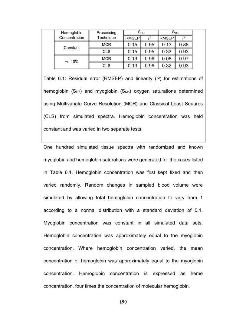
190
One hundred simulated tissue spectra with randomized and known
myoglobin and hemoglobin saturations were generated for the cases listed
in Table 6.1. Hemoglobin concentration was first kept fixed and then
varied randomly. Random changes in sampled blood volume were
simulated by allowing total hemoglobin concentration to vary from 1
according to a normal distribution with a standard deviation of 0.1.
Myoglobin concentration was constant in all simulated data sets.
Hemoglobin concentration was approximately equal to the myoglobin
concentration. Where hemoglobin concentration varied, the mean
concentration of hemoglobin was approximately equal to the myoglobin
concentration. Hemoglobin concentration is expressed as heme
concentration, four times the concentration of molecular hemoglobin.
RMSEP r2 RMSEP r
2
MCR 0.15 0.95 0.13 0.88
CLS 0.15 0.95 0.33 0.93
MCR 0.13 0.96 0.08 0.97
CLS 0.13 0.96 0.32 0.93
Constant
+/- 10%
Hemoglobin
Concentration
Processing
Technique
SHb SMb
Table 6.1: Residual error (RMSEP) and linearity (r2) for estimations of
hemoglobin (SHb) and myoglobin (SMb) oxygen saturations determined
using Multivariate Curve Resolution (MCR) and Classical Least Squares
(CLS) from simulated spectra. Hemoglobin concentration was held
constant and was varied in two separate tests.
191
A third series of tissue simulation spectra were developed to
determine the minimum oxygen saturation range required for accurate
estimation of myoglobin oxygen saturation. The data set must contain
some perturbation in order for MCR to successfully separate the spectral
components. Simulated spectral data included fixed total myoglobin
concentration, and allowed total hemoglobin concentration to vary by 10%.
Since it is expected that normal SMb values in the heart are close to
100%,97 each set of simulated tissue spectra spanned a range from 100 %
to a lower bound which varied from 99% to 60% in increments of 1%.
Hemoglobin saturation was varied over the same saturation range as
myoglobin. Results for each saturation range were evaluated from the
average performance over 10 tissue simulation data sets, each containing
100 spectra.
6.7.2 Cardiac Tissue Data
All animal protocols were approved by the Institutional Animal Care
and Use Committee at the University of Washington. Optical
spectroscopic measurements of guinea pig hearts (n = 9) were recorded
between 450 and 950 nm. Excised hearts were perfused with red blood
cells at 5% hematocrit under conditions of varying oxygen saturation
according to the Langendorff method. Diffuse reflectance spectra were
192
recorded from the left ventricular wall using a custom bifurcated fiber optic
probe having a 1.75 mm separation between source and detector fibers.
Spectra of cardiac tissue were collected as previously described in
detail.232, 244 Spectra were recorded for each excised heart while oxygen
saturation of the blood was controlled using a gas-exchange perfusion
system to control the oxygen, nitrogen and carbon dioxide concentrations.
Each heart was exposed to a hypoxic ramp over 20 minutes, a linear
reduction in perfusate oxygen content. Maximum myoglobin oxygen
saturation was produced experimentally by perfusion with oxygenated
buffer, infusion of adenosine to maximally vasodilate the coronary arteries,
and infusion of potassium chloride to arrest the heart and thus lower
myocardial oxygen consumption. Maximal deoxygenation was produced
by infusion of sodium dithionite (Na2SO4) at the end of each experiment.244
Guinea pig heart spectra were pre-processed by taking second derivatives
with the same settings as used for tissue simulation spectra. All spectral
analyses were done in the range from 450 to 650 nm.
6.8 Results & Discussion
To evaluate the use of the MCR method for measuring myoglobin
oxygen saturation, both simulated and cardiac tissue spectra were
examined. Estimates of oxygen saturation using MCR and CLS were
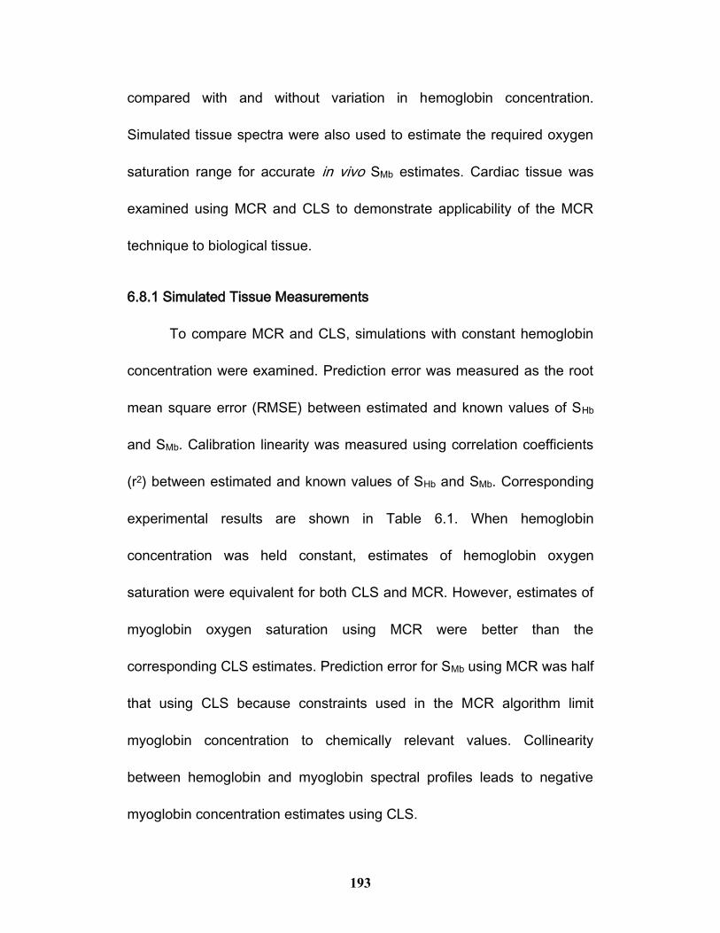
193
compared with and without variation in hemoglobin concentration.
Simulated tissue spectra were also used to estimate the required oxygen
saturation range for accurate in vivo SMb estimates. Cardiac tissue was
examined using MCR and CLS to demonstrate applicability of the MCR
technique to biological tissue.
6.8.1 Simulated Tissue Measurements
To compare MCR and CLS, simulations with constant hemoglobin
concentration were examined. Prediction error was measured as the root
mean square error (RMSE) between estimated and known values of SHb
and SMb. Calibration linearity was measured using correlation coefficients
(r2) between estimated and known values of SHb and SMb. Corresponding
experimental results are shown in Table 6.1. When hemoglobin
concentration was held constant, estimates of hemoglobin oxygen
saturation were equivalent for both CLS and MCR. However, estimates of
myoglobin oxygen saturation using MCR were better than the
corresponding CLS estimates. Prediction error for SMb using MCR was half
that using CLS because constraints used in the MCR algorithm limit
myoglobin concentration to chemically relevant values. Collinearity
between hemoglobin and myoglobin spectral profiles leads to negative
myoglobin concentration estimates using CLS.
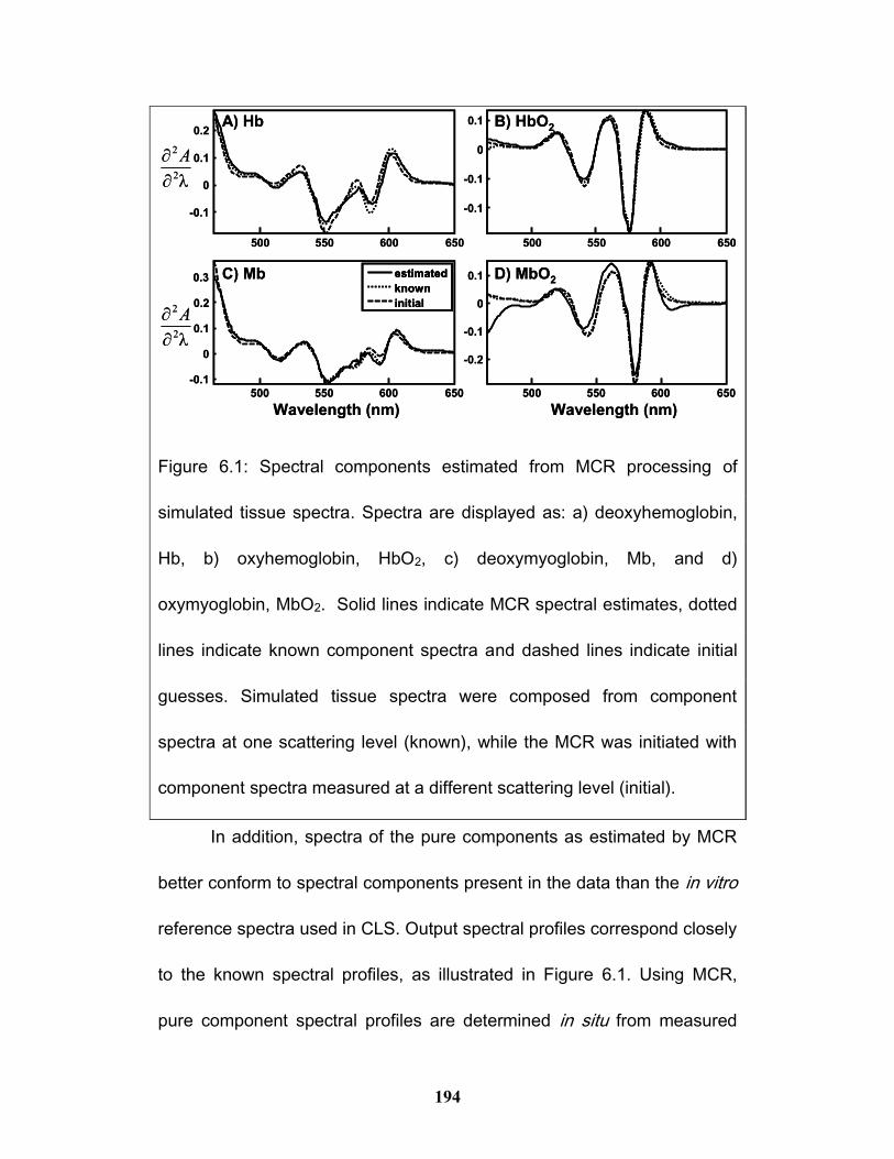
194
In addition, spectra of the pure components as estimated by MCR
better conform to spectral components present in the data than the in vitro
reference spectra used in CLS. Output spectral profiles correspond closely
to the known spectral profiles, as illustrated in Figure 6.1. Using MCR,
pure component spectral profiles are determined in situ from measured
500 550 600 650
-0.1
0
0.1
500 550 600 650
-0.1
0
0.1
500 550 600 650
-0.1
0
0.1
500 550 600 650
-0.1
0
0.1estimated
known
initial
A) Hb B) HbO2
C) Mb D) MbO2
Wavelength (nm) Wavelength (nm)
2
2A
2
2A
0.2
0.2
0.3
-0.1
-0.2
500 550 600 650
-0.1
0
0.1
500 550 600 650
-0.1
0
0.1
500 550 600 650
-0.1
0
0.1
500 550 600 650
-0.1
0
0.1estimated
known
initial
estimated
known
initial
A) Hb B) HbO2
C) Mb D) MbO2
Wavelength (nm) Wavelength (nm)
2
2A
2
2A
0.2
0.2
0.3
-0.1
-0.2
Figure 6.1: Spectral components estimated from MCR processing of
simulated tissue spectra. Spectra are displayed as: a) deoxyhemoglobin,
Hb, b) oxyhemoglobin, HbO2, c) deoxymyoglobin, Mb, and d)
oxymyoglobin, MbO2. Solid lines indicate MCR spectral estimates, dotted
lines indicate known component spectra and dashed lines indicate initial
guesses. Simulated tissue spectra were composed from component
spectra at one scattering level (known), while the MCR was initiated with
component spectra measured at a different scattering level (initial).
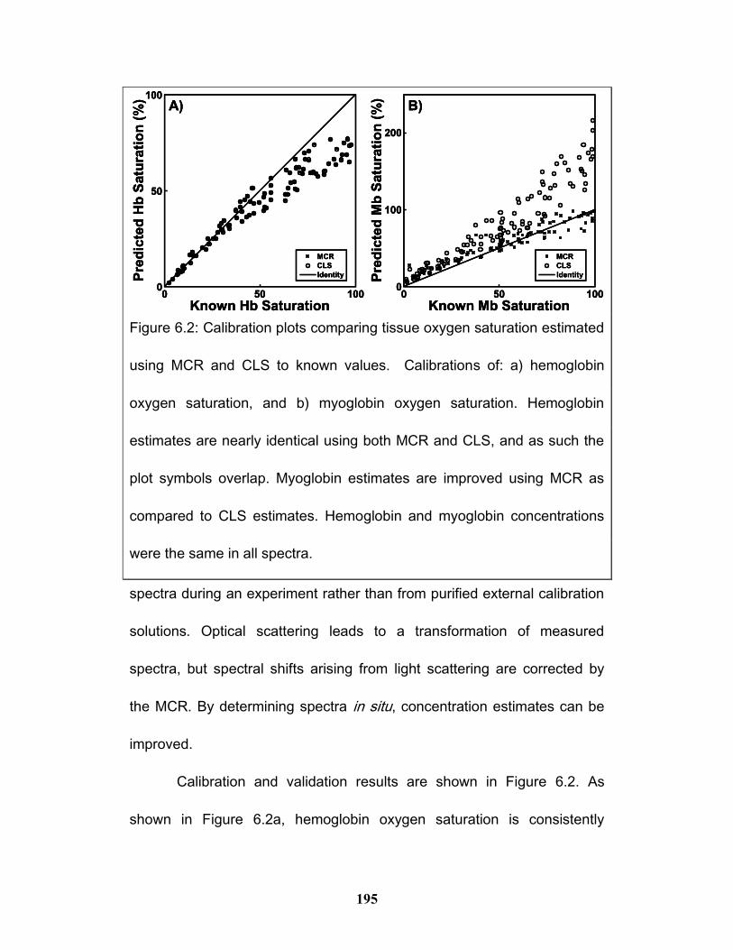
195
spectra during an experiment rather than from purified external calibration
solutions. Optical scattering leads to a transformation of measured
spectra, but spectral shifts arising from light scattering are corrected by
the MCR. By determining spectra in situ, concentration estimates can be
improved.
Calibration and validation results are shown in Figure 6.2. As
shown in Figure 6.2a, hemoglobin oxygen saturation is consistently
500
100
200
Pre
dic
ted
Mb
Satu
rati
on
(%
)
Known Mb Saturation
Identity
MCR
CLS
0 100
B)
0 1000
100
Identity
MCR
CLS
Pre
dic
ted
Hb
Satu
rati
on
(%
)
Known Hb Saturation50
A)
50
500
100
200
Pre
dic
ted
Mb
Satu
rati
on
(%
)
Known Mb Saturation
Identity
MCR
CLS
0 100
B)
500
100
200
Pre
dic
ted
Mb
Satu
rati
on
(%
)
Known Mb Saturation
Identity
MCR
CLS
0 100
B)
0 1000
100
Identity
MCR
CLS
Pre
dic
ted
Hb
Satu
rati
on
(%
)
Known Hb Saturation50
A)
50
0 1000
100
Identity
MCR
CLS
Pre
dic
ted
Hb
Satu
rati
on
(%
)
Known Hb Saturation50
A)
50
Figure 6.2: Calibration plots comparing tissue oxygen saturation estimated
using MCR and CLS to known values. Calibrations of: a) hemoglobin
oxygen saturation, and b) myoglobin oxygen saturation. Hemoglobin
estimates are nearly identical using both MCR and CLS, and as such the
plot symbols overlap. Myoglobin estimates are improved using MCR as
compared to CLS estimates. Hemoglobin and myoglobin concentrations
were the same in all spectra.
196
estimated by both CLS and MCR. However, as shown in Figure 6.2b, the
CLS method overestimates myoglobin oxygen saturation. Using the
closure constraint, MCR corrects the overestimates. Hemoglobin spectral
intensity in the measured pure components is about 30% greater than the
myoglobin spectral intensity. Noise added to the simulation degrades
myoglobin concentration estimates more than the hemoglobin
concentration estimates because of the difference in the spectral
weightings. In cases where the total spectral intensity from myoglobin is
much greater than from hemoglobin, hemoglobin concentration estimates
become worse than the myoglobin concentration estimates. Regardless of
the relative component magnitudes, oxygen saturation estimates are
improved when using the MCR routine.
When hemoglobin concentration was varied in the simulated
spectra, the error in MCR estimates of SMb was less than when
hemoglobin concentration was fixed, and linearity increased slightly. In
contrast, when using CLS for estimation of SMb, error and linearity were
constant regardless of hemoglobin variation. These results indicate that
variation of hemoglobin perfusion improves the capacity for the MCR
algorithm to adapt pure spectra to data. This is fortuitous, as hemoglobin
perfusion varies naturally with both time and oxygenation. It appears that
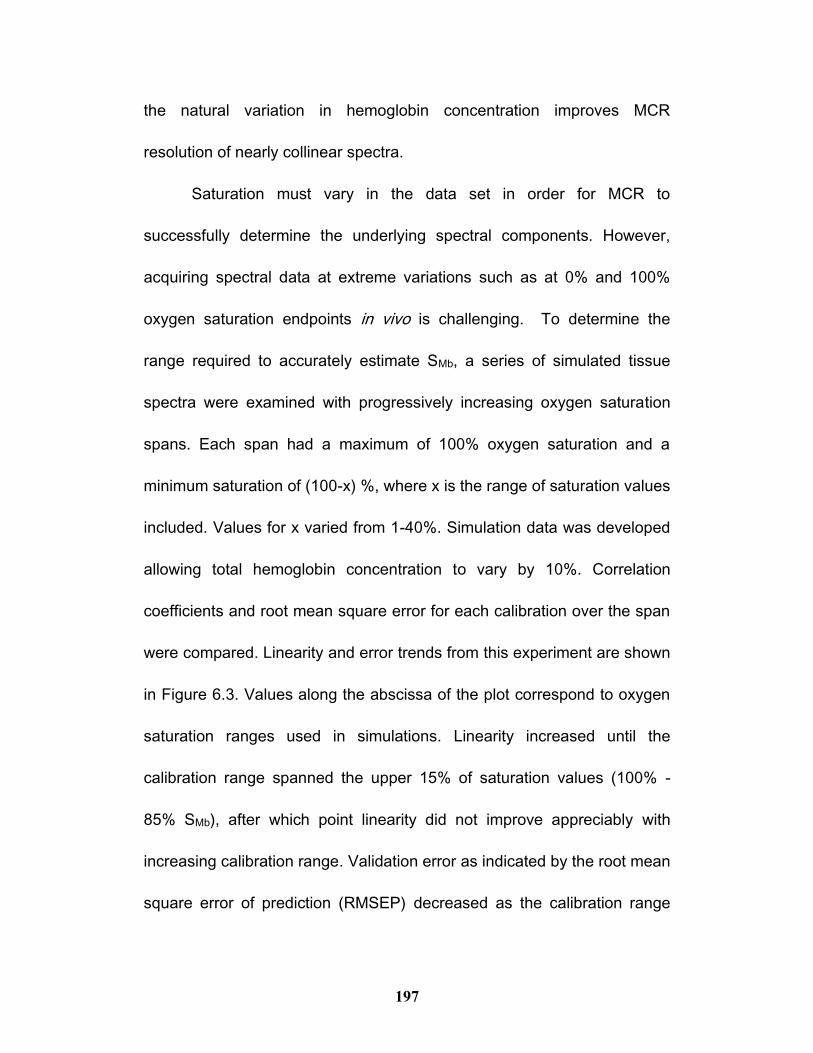
197
the natural variation in hemoglobin concentration improves MCR
resolution of nearly collinear spectra.
Saturation must vary in the data set in order for MCR to
successfully determine the underlying spectral components. However,
acquiring spectral data at extreme variations such as at 0% and 100%
oxygen saturation endpoints in vivo is challenging. To determine the
range required to accurately estimate SMb, a series of simulated tissue
spectra were examined with progressively increasing oxygen saturation
spans. Each span had a maximum of 100% oxygen saturation and a
minimum saturation of (100-x) %, where x is the range of saturation values
included. Values for x varied from 1-40%. Simulation data was developed
allowing total hemoglobin concentration to vary by 10%. Correlation
coefficients and root mean square error for each calibration over the span
were compared. Linearity and error trends from this experiment are shown
in Figure 6.3. Values along the abscissa of the plot correspond to oxygen
saturation ranges used in simulations. Linearity increased until the
calibration range spanned the upper 15% of saturation values (100% -
85% SMb), after which point linearity did not improve appreciably with
increasing calibration range. Validation error as indicated by the root mean
square error of prediction (RMSEP) decreased as the calibration range

198
increased. Saturation ranges greater than 15% did not show appreciable
improvement of RMSEP. These results suggest that a minimum
calibration range spanning from 85% to 100% SMb should be sampled for
calibration of SMb by MCR in cardiac tissue. This range of oxygen content
is feasible, and SMb values such as these should be attainable by variation
of the oxygen content of inspired air.134
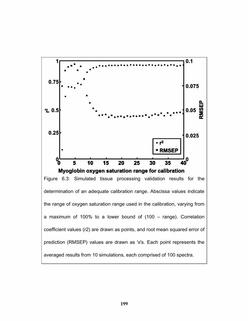
199
0 5 10 15 20 25 30 35 400
0.5
1
r2
0 5 10 15 20 25 30 35 400
0.05
0.1
Myoglobin oxygen saturation range for calibration
RM
SE
P
r2
RMSEP
0 5 10 15 20 25 30 35 40
r2
0 5 10 15 20 25 30 35 40
Myoglobin oxygen saturation range for calibration
RM
SE
P
r2
RMSEP
0.25
0.750.075
0.025
0 5 10 15 20 25 30 35 400
0.5
1
r2
0 5 10 15 20 25 30 35 400
0.05
0.1
Myoglobin oxygen saturation range for calibration
RM
SE
P
r2
RMSEP
0 5 10 15 20 25 30 35 40
r2
0 5 10 15 20 25 30 35 40
Myoglobin oxygen saturation range for calibration
RM
SE
P
r2
RMSEP
0.25
0.750.075
0.025
Figure 6.3: Simulated tissue processing validation results for the
determination of an adequate calibration range. Abscissa values indicate
the range of oxygen saturation range used in the calibration, varying from
a maximum of 100% to a lower bound of (100 – range). Correlation
coefficient values (r2) are drawn as points, and root mean squared error of
prediction (RMSEP) values are drawn as 'x's. Each point represents the
averaged results from 10 simulations, each comprised of 100 spectra.
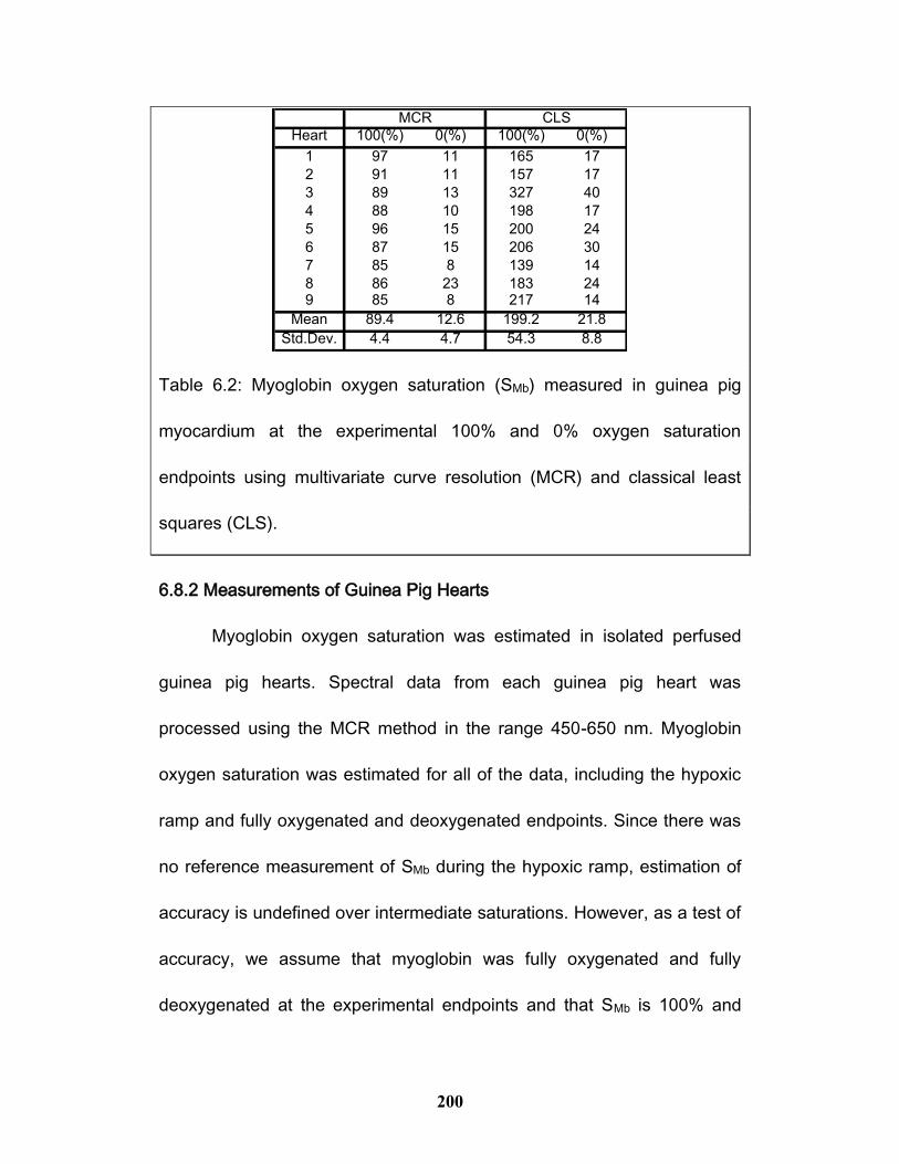
200
6.8.2 Measurements of Guinea Pig Hearts
Myoglobin oxygen saturation was estimated in isolated perfused
guinea pig hearts. Spectral data from each guinea pig heart was
processed using the MCR method in the range 450-650 nm. Myoglobin
oxygen saturation was estimated for all of the data, including the hypoxic
ramp and fully oxygenated and deoxygenated endpoints. Since there was
no reference measurement of SMb during the hypoxic ramp, estimation of
accuracy is undefined over intermediate saturations. However, as a test of
accuracy, we assume that myoglobin was fully oxygenated and fully
deoxygenated at the experimental endpoints and that SMb is 100% and
Heart 100(%) 0(%) 100(%) 0(%)
1 97 11 165 17
2 91 11 157 17
3 89 13 327 40
4 88 10 198 17
5 96 15 200 24
6 87 15 206 30
7 85 8 139 14
8 86 23 183 249 85 8 217 14
Mean 89.4 12.6 199.2 21.8
Std.Dev. 4.4 4.7 54.3 8.8
MCR CLS
Table 6.2: Myoglobin oxygen saturation (SMb) measured in guinea pig
myocardium at the experimental 100% and 0% oxygen saturation
endpoints using multivariate curve resolution (MCR) and classical least
squares (CLS).
201
0%, respectively, during these periods. Saturation estimates for nine
hearts using MCR and CLS are displayed in Table 6.2. CLS values at the
100% SMb endpoint were physically impossible because they exceeded
100% saturation. This artifact was caused by negative deoxymyoglobin
concentration estimates. Using MCR, concentration estimates were
constrained to a physically possible range using non-negativity
constraints. Concentrations were related using closure (Eq. 6.5) to
compute SMb (Eq. 6.6). Typical values of the closure constraint, k, ranged
from 1 to 4 when processing guinea pig heart spectra. Composition of
deoxymyoglobin and oxymyoglobin components after scaling for closure is
shown in Figure 6.4 for one heart. In a typical hypoxic ramp, MCR
estimates showed decreases in oxymyoglobin concentration and
increases in deoxymyoglobin concentration. Values measured at the 0%
and 100% saturation values are plotted as the two final points. Endpoint
saturations estimated by MCR are nearer to the ideal saturations than
CLS estimates (Table 2).
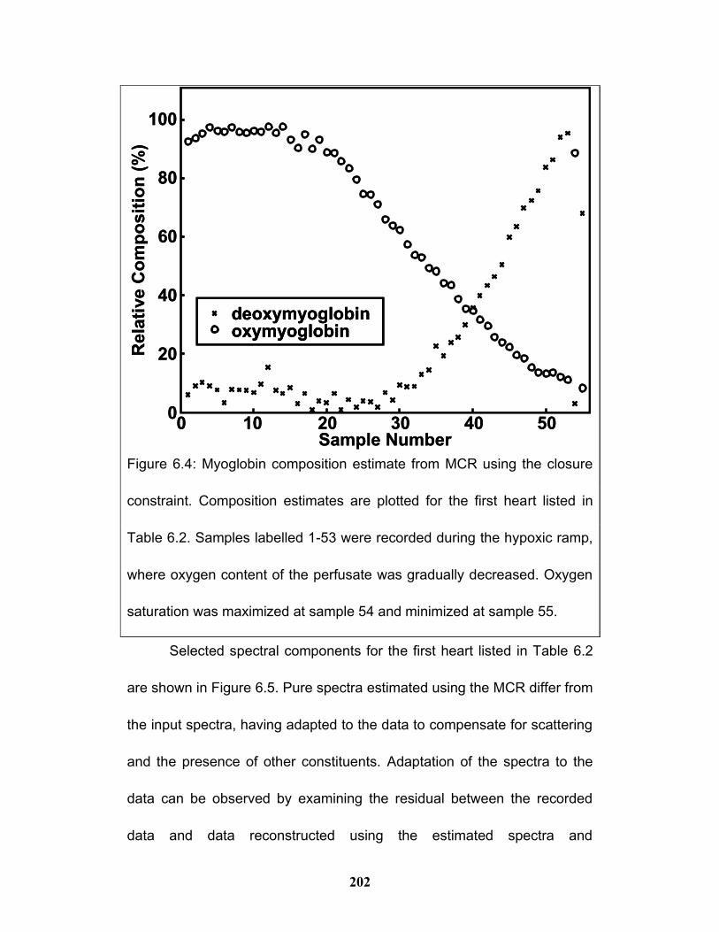
202
Selected spectral components for the first heart listed in Table 6.2
are shown in Figure 6.5. Pure spectra estimated using the MCR differ from
the input spectra, having adapted to the data to compensate for scattering
and the presence of other constituents. Adaptation of the spectra to the
data can be observed by examining the residual between the recorded
data and data reconstructed using the estimated spectra and
0 10 20 30 40 500
Sample Number
Rela
tive C
om
po
sit
ion
(%
)
deoxymyoglobinoxymyoglobin
20
40
60
80
100
0 10 20 30 40 500
Sample Number
Rela
tive C
om
po
sit
ion
(%
)
deoxymyoglobinoxymyoglobindeoxymyoglobinoxymyoglobin
20
40
60
80
100
Figure 6.4: Myoglobin composition estimate from MCR using the closure
constraint. Composition estimates are plotted for the first heart listed in
Table 6.2. Samples labelled 1-53 were recorded during the hypoxic ramp,
where oxygen content of the perfusate was gradually decreased. Oxygen
saturation was maximized at sample 54 and minimized at sample 55.
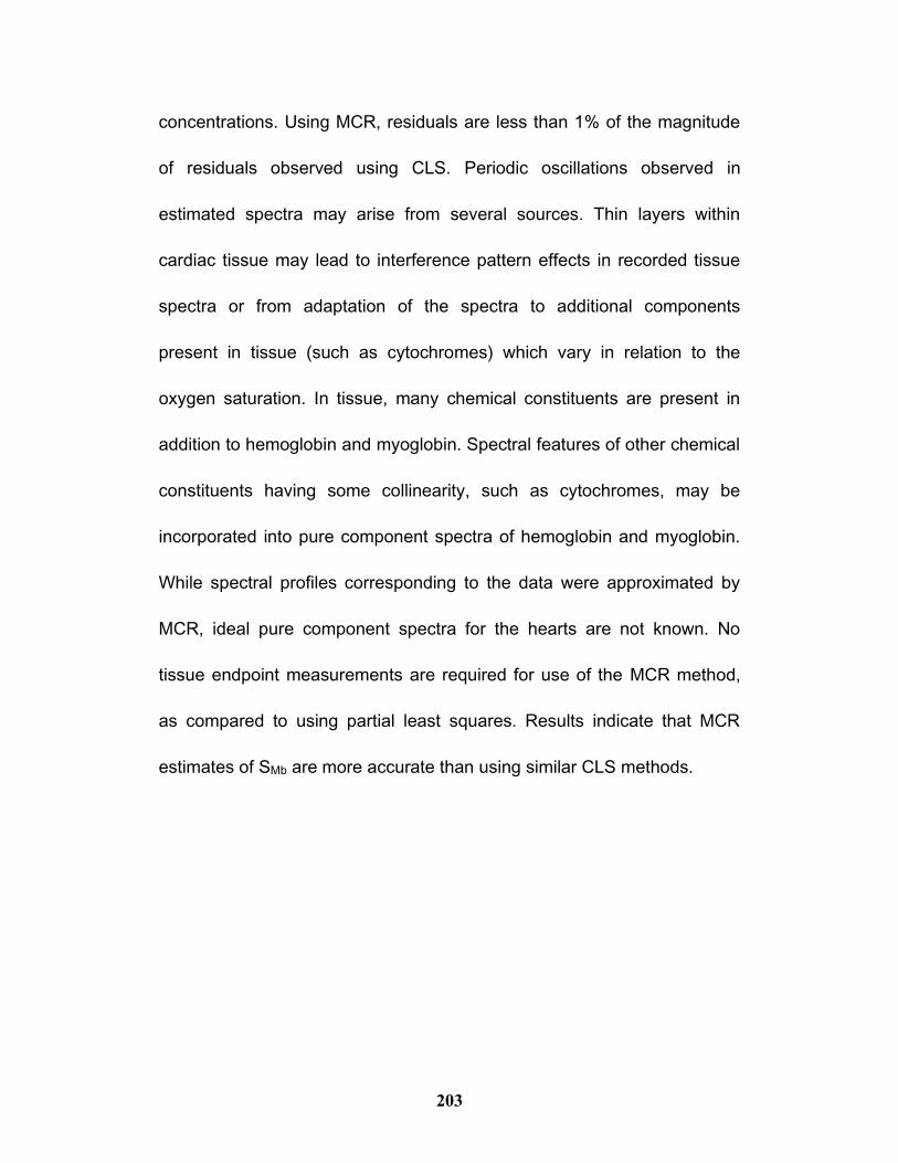
203
concentrations. Using MCR, residuals are less than 1% of the magnitude
of residuals observed using CLS. Periodic oscillations observed in
estimated spectra may arise from several sources. Thin layers within
cardiac tissue may lead to interference pattern effects in recorded tissue
spectra or from adaptation of the spectra to additional components
present in tissue (such as cytochromes) which vary in relation to the
oxygen saturation. In tissue, many chemical constituents are present in
addition to hemoglobin and myoglobin. Spectral features of other chemical
constituents having some collinearity, such as cytochromes, may be
incorporated into pure component spectra of hemoglobin and myoglobin.
While spectral profiles corresponding to the data were approximated by
MCR, ideal pure component spectra for the hearts are not known. No
tissue endpoint measurements are required for use of the MCR method,
as compared to using partial least squares. Results indicate that MCR
estimates of SMb are more accurate than using similar CLS methods.
204
6.9 Conclusions
Myoglobin oxygen saturation (SMb) is more accurately measured
from visible spectra using multivariate curve resolution (MCR) than by
classical least squares (CLS). Pure spectral profiles were estimated using
the MCR algorithm, and quantification was improved through application
of constraints tailored to the system under study. Incorporation of
pre-processing steps may yield constraints that are invalid, and
-0.1
0
0.1
500 550 600 650
2
2A
A) Hb0.2
-0.1
0
0.2
Wavelength (nm)500 550 600 650
2
2A
C) Mb
0.1
0.3
-0.2
-0.1
0
0.1
500 550 600 650
B) HbO2
-0.2
-0.1
0
0.1
Wavelength (nm)500 550 600 650
D) MbO2
-0.2
-0.1
0
0.1
500 550 600 650
2
2A
A) Hb0.2
-0.1
0
0.1
500 550 600 650
2
2A
A) Hb0.2
-0.1
0
0.2
Wavelength (nm)500 550 600 650
2
2A
C) Mb
0.1
0.3
-0.2
-0.1
0
0.2
Wavelength (nm)500 550 600 650
2
2A
C) Mb
0.1
0.3
-0.2
-0.1
0
0.1
500 550 600 650
B) HbO2
-0.2
-0.1
0
0.1
500 550 600 650
B) HbO2
-0.2
-0.1
0
0.1
Wavelength (nm)500 550 600 650
D) MbO2
-0.2
-0.1
0
0.1
Wavelength (nm)500 550 600 650
D) MbO2
-0.2
Figure 6.5: Spectral profiles estimated for the first guinea pig heart listed in
Table 2 using the MCR algorithm. Estimated spectral profiles are shown
as solid curves, while the initial spectra input to the MCR are shown as
dotted curves. Spectra are displayed as: a) deoxyhemoglobin, Hb, b)
oxyhemoglobin, HbO2, c) deoxymyoglobin, Mb, and d) oxymyoglobin,
MbO2.
205
pre-processing steps should be optimized against physical constraints. In
particular, MCR is useful when known pure spectral profiles are modified
by scattering or when they cannot be measured in isolation. Myoglobin
oxygen saturation in tissue can be estimated without recording endpoint
spectra for calibration and normalization in each data set. Instead, a
closure constraint is automatically determined from recorded data to
determine the proper scaling of component concentrations for SMb
estimates. Simulations indicate that in order to use the MCR technique,
the spectral data set must include myoglobin saturation values that vary
from at least 85% to 100%. Suitable oxygen saturation ranges should be
possible under normal physiological conditions through manipulations of
inspired oxygen content. Finally, results showed that variations in
hemoglobin concentration seem to improve myoglobin oxygen saturation
measurements.
206
Chapter 7. Conclusions and Future Work
Spectroscopy is a powerful method for analyzing a variety of
materials, through which chemically specific information can be obtained
non-invasively. Despite the large body of research into non-invasive tissue
measurements using diffuse-reflectance NIR spectroscopy, it is not yet
commonly used. One of the main limitations is the lack of optimal
correction for light scattering. This dissertation has described four practical
methods for correcting light scattering in order to better quantify analyte
concentrations in turbid media.
As explained throughout this thesis, light scattering is deleterious to
accurate in situ diffuse-reflectance measurements. The theory and
practice of diffuse-reflectance is difficult because the most commonly used
spectroscopic model of light absorbance, the Lambert-Beer law, does not
account for light scattering. More complex models of photon transport,
such as the radiative transport equation and its diffusion approximation
treat multiple scattering. These models serve as a theoretical basis to
correct for scattering effects. Experimental approaches have been
developed to measure optical properties, such as the absorption
coefficient, and to use measured reduced scattering coefficients for
improving spectroscopic quantification in turbid media.
207
7.1 Conclusions
This thesis has focused on four methods for improving
spectroscopy in scattering media. These practical methods are applicable
to biomedical spectroscopy for point and imaging measurements.
Depending on the particular application, either point measurements or
imaging measurements are used.
Point measurements are appropriate for the evaluation of chemical
composition at a single location of interest or in cases where
concentrations change relatively slowly. Applications which use point
measurements include studies for identifying lesions or tissue damage,
and studies for quantifying lactate, glucose, or oxygen saturation. An
advantage of point measurements is that relatively simple instruments can
be built to fulfil these applications. Single-point spectroscopic measures
can be improved using photon time-of-flight instruments. For example, the
photon time-of-flight instrument described in chapter 3 is appropriate for
point measurements of the reduced scattering coefficient.
In chapter 3, a rapid handheld time-of-flight spectrometer was
demonstrated for measuring the scattering coefficient. A spectrum
recorded with a commercially available handheld spectrometer was
corrected using the scattering coefficient measured with the photon time-
208
of-flight instrument. This was shown to improve quantification of dye in a
turbid sample using a single-point optical measure by 35%. This
instrument is practical for improving point-spectroscopy measures in
tissue.
In chapter 5, a method was described for incorporating generic
parsimony or simplicity measures into genetic algorithms for automated
data processing method development. This approach is useful for
developing simplified spectroscopic systems, and might be incorporated
with the photon time-of-flight instrument to develop optimal point-
measurement devices. Potential applications for handheld medical
devices include measurement of hemoglobin and myoglobin oxygen
saturation, lactate and glucose concentration, and evaluation of burns,
edema and other disease states. Parsimonious genetic algorithms are
useful for identifying important wavelength regions and for guiding the
development of optimal devices. By combining a readily available portable
spectrometer and the portable photon time-of-flight instrument, the
parsimonious genetic algorithm can be used to efficiently develop new
analytical spectroscopy methods. The genetic algorithm was shown to
improve quantification of lactate in vivo by 20% as compared to the best
method developed by an expert.
209
Imaging spectral measurements are appropriate for measurements
of heterogeneous systems such as: to identify regions of interest, for
measuring rapidly varying concentrations, and for measuring the
properties of tissues in motion (in cardiac tissue for example).
To improve spectroscopic imaging, a novel instrument was
demonstrated using images of an annular illumination pattern projected
onto a sample surface to estimate the reduced scattering coefficient.
Imaging annular laser patterns to estimate scattering holds several
advantages with respect to imaging Gaussian beams. Most important is
the short source-detector separation distance (ρ) used in this method.
Illumination intensity is distributed over a larger area as compared to
Gaussian beam imaging methods, decreasing the flux while maintaining
the same illumination power. In order to measure the optical absorbance
of components within the scattering medium, reference reflectance
intensity must be determined. Reflectance is a function of the scattering
coefficient, and the reference reflectance can be estimated from the
measured scattering coefficient. Chapter 4 describes how reflectance at
the center and edges of the annular laser pattern can be used to first
measure the scattering coefficient, and also how to use the scattering
coefficient to estimate the reference reflectance intensity. Finally, the
210
absorption coefficient can be estimated using the measured reflectance
(with absorbance) and the estimated reference reflectance (absorbance-
free). Using the annular beam imaging method, error in the estimation of
absorption coefficients was reduced by 50% as compared to conventional
imaging.
In chapter 6, multivariate curve resolution method is used to
estimate constituent concentrations and spectra directly from the spectra
of a series of mixtures. This approach is applicable towards modelling of
imaging data, and might be incorporated into the annular imaging system
to develop improved spectroscopic imaging systems. Multivariate curve
resolution leverages the variance within a data set to estimate underlying
spectral components. In imaging spectroscopy the composition may vary
with position in the image. The rapid multivariate curve resolution
algorithm shows promise for real-time spectral processing and adaptive
modelling. In chapter 6 we demonstrated that over the clinically relevant
oxygen saturation range of 85-100% the multivariate curve resolution
approach estimated myoglobin oxygen saturation more accurately than
the classical least squares approach.
211
7.2 Future Work
Potential avenues of future research are proposed in this section,
where improvements can be made to each technique individually.
Moreover, the various techniques can be combined to achieve further
improvements. Improvements in efficiency, accuracy, and ease-of-use
would advance the use of clinical non-invasive reflectance spectroscopy.
7.2.1 Future Work using the Photon Time-of-Flight Instrument
With improvements to this portable time-of-flight system, more
accurate estimations of μs' will enable more precise quantification of
components in highly scattering media. Several methods are proposed
here for improving upon the current system, these include improvements
using the current system, and improvements through modification of the
current electronics.
Without any modification of the current electronics, a shorter pulse
can be used. The current system can be reconfigured in software to output
a 5 or 10 nanosecond pulse. Using a 10 nanosecond pulse should not
decrease the peak intensity. With a 5 nanosecond pulse, optical intensity
would decrease, though the temporal shift would be even more
pronounced, likewise, skew and kurtosis would be more prominent. An
increase in the pulse rate should also permit faster measurements by
212
allowing for decreased signal-averaging times. A second set of
improvements requiring changes to the electronics of the device would be
to use higher charge and gate voltages to the laser diodes. The optical
output of the laser diodes may be increased three- or four-fold by
optimizing the charge and gate voltages. A third method would involve
improvement of the detection system. The rise time of the detector could
be decreased by increasing the reverse bias applied to the diode.
Likewise, the use of a high-speed amplifier could increase the absolute
magnitude of the detected electrical signal and thus improve the signal-to-
noise ratio of the time-of-flight profiles. The bandwidth of the oscilloscope
was only 200 MHz, and coupling between the channels was observed to
cause ringing. Simplified electronics could be incorporated to replace the
oscilloscope. Previously unpublished results illustrate the utility of
decimation of the temporal profiles by electronically windowing the
electrical signal from the detector with a delayed trigger pulse using digital
delay lines and a high-speed mixer. Likewise the oscilloscope used an 8-
bit analog-to-digital converter, whereas a 12- or 16-bit analog-to-digital
converter would improve the precision of the digitization. Finally, it should
be noted that voltages for the laser control circuitry were chosen for
convenience of design and construction. This system was designed to run
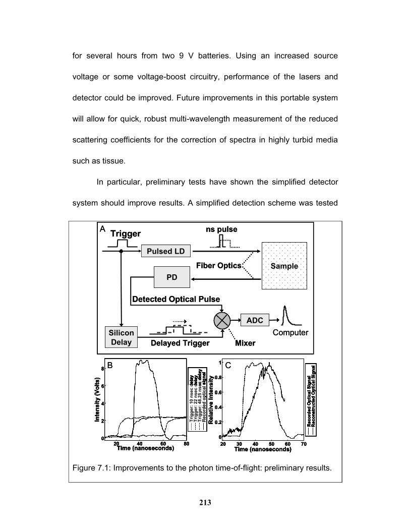
213
for several hours from two 9 V batteries. Using an increased source
voltage or some voltage-boost circuitry, performance of the lasers and
detector could be improved. Future improvements in this portable system
will allow for quick, robust multi-wavelength measurement of the reduced
scattering coefficients for the correction of spectra in highly turbid media
such as tissue.
In particular, preliminary tests have shown the simplified detector
system should improve results. A simplified detection scheme was tested
ns pulse
PD
Detected Optical Pulse
Trigger
Silicon
Delay Delayed Trigger
Pulsed LD
Computer
SampleFiber Optics
ADC
Mixer
20 30 40 50 60 70
0
0.2
0.4
0.6
0.8
1
Time (nanoseconds)
Rela
tiv
e I
nte
ns
ity
Reco
rded
Op
tical
Sig
nal
Reco
nstr
ucte
d O
pti
cal
Sig
nal
20 30 40 50 60 70
0
0.2
0.4
0.6
0.8
1
Time (nanoseconds)
Rela
tiv
e I
nte
ns
ity
Reco
rded
Op
tical
Sig
nal
Reco
nstr
ucte
d O
pti
cal
Sig
nal
Reco
rded
Op
tical
Sig
nal
Reco
nstr
ucte
d O
pti
cal
Sig
nal
20 40 60 800
2
4
6
8
Time (nanoseconds)
Inte
nsit
y (
Vo
lts
)
Tri
gg
er:
10 n
sec
de
lay
Tri
gg
er:
22 n
sec
de
lay
Tri
gg
er:
48.2
5 n
sec
de
lay
Rec
ord
ed
op
tic
al
sig
na
l
20 40 60 800
2
4
6
8
Time (nanoseconds)
Inte
nsit
y (
Vo
lts
)
Tri
gg
er:
10 n
sec
de
lay
Tri
gg
er:
22 n
sec
de
lay
Tri
gg
er:
48.2
5 n
sec
de
lay
Rec
ord
ed
op
tic
al
sig
na
l
Tri
gg
er:
10 n
sec
de
lay
Tri
gg
er:
22 n
sec
de
lay
Tri
gg
er:
48.2
5 n
sec
de
lay
Rec
ord
ed
op
tic
al
sig
na
l
A
B C
Figure 7.1: Improvements to the photon time-of-flight: preliminary results.
214
using a variable delay line (DS1040, Maxim Integrated Products, Inc., CA,
USA) and a signal mixer (ZAD-1, Mini-Circuits, New York, USA) to
transform the optical signal output from the high speed silicon photodiode.
A diagram of the simplified detector system is shown in Figure 7.1. For
testing purposes, the output was recorded using the high speed
oscilloscope. The digital delay line was fed with the laser trigger pulse,
and the delayed trigger selected a temporal window from the optical
signal. The mixer transforms (inverts) the detected optical pulse using the
delayed trigger. Signal from the mixer was recorded for each of the 256
time-steps of the delay line, as shown in Figure 7.1. The detected signal
includes a background ringing signal caused by the laser module. By
taking the sum of intensity in each trace, the integrated signal was
estimated for each time delay. Integrated signal was plotted against delay
time and reconstructed of the directly measured optical pulse. Preliminary
results are shown in Figure 7.1, where the reconstructed pulse is shown
along with the directly measured pulse. While distortion is present, major
features of the time-of-flight profile are present. Initial tests were
laboriously carried out by manually selecting the delay-time and recording
the oscilloscope trace. In the next iteration of the simplified photon time-of-
flight instrument, the delay-time will be digitally selected using a
215
microcontroller that will also record the signal magnitude as averaged
across a capacitor. The automated system should allow a complete
measurement of the photon time-of-flight profile in a quarter of a second
with a temporal resolution of 150 picoseconds. Furthermore, the
intensities would be recorded using 12- or 16-bit analog to digital
converters rather than an 8-bit analog to digital converter. As a result, the
next iteration of the time-of-flight instrument should have a two order of
magnitude improvement in signal resolution. With these improvements, a
portable biomedical instrument should be feasible.
7.2.2 Future Work using the Ring-Light System
A natural extension of the ring imaging technique is to examine the
effects of a variable ring diameter. Source-detector separation distance is
known to change the optical sampling depth.245, 246 Variation of ring
diameter may allow depth-resolved non-invasive measurement of
scattering properties. In the current work, reduced scattering coefficients
were measured within the ring source pattern. In future experiments, ring
diameter can be dynamically controlled using a spatial light modulator or
adjustable conical lenses to measure scattering at different sampling
depths. In the recently reported subsurface Raman ring/disk spectroscopy,
ring patterns were formed using conical lenses to transform the incident
216
Gaussian laser beam into a ring-shape.173, 174 Illumination ring diameter
was varied by adjusting the position of the conic lens, or using adjustable
telescopic lenses.173, 174 This combination has shown sensitivity to
depth.247, 248 Combinations of ring arrays and dynamic diameter selection
have the potential to map subsurface scattering properties. Depth
penetration increases as ρ increases, as does the sampling volume, which
scales approximately as the cube of the source-detector separation. Using
computer-generated holograms arrays of annular patterns can be
produced. Arrays of rings might be used to measure the optical properties
at many positions over a surface. Imaging annular arrays would allow
scattering properties to be measured at many spatial positions
concurrently. This imaging technique should ultimately allow non-invasive
tomographic imaging spectroscopy of highly turbid media.
Aspects to examine for improving the annular measurements
should include verification of the effects of changing anisotropy, testing the
accuracy when mapping scattering coefficients using an array of rings,
and testing whether variations of the ring diameter can be used to
measure depth-resolved scattering coefficients. One experimental method
for controlling anisotropy is to vary the refractive index of the solution,
while using a constant scattering particle size and concentration. By using
217
polystyrene/latex microspheres and different solvents the anisotropy can
be controlled, while keeping the scattering coefficient constant.
Experimental methods for testing imaging with multiple rings and depth-
dependence could use scattering spheres embedded in thin slices of
polymer. Additionally, the system should be tested with the camera at
greater distances, particularly for any future medical applications.
7.2.3 Future Work using the Genetic Algorithm
Genetic algorithms are well suited for the selection of data
processing methods which can be used to guide the design of portable
instruments. Future directions for improving genetic algorithms in
processing method selection should consider better ways of incorporating
preprocessing step complexity into parsimony penalties, better ways of
determining optimal cross-validation group sizes, and improved methods
for selecting between the final solutions presented by the GA. Metrics for
improving the assessment of model complexity include the time or
memory required for processing, algorithm complexity using 'O-notation',
or a financial cost for building a simplified instrument using the specified
model (by including instrument costs for component such as specialized
optical filters and the number of detectors). Ideally, non-parametric
statistical methods should be used for comparing model size and
218
preprocessing step complexity, along with different complexity metrics.
Cross-validation group sizes need to be better studied so that the
accuracy of cross-validated model performance metrics is better
understood. Statistical properties of cross-validated results are difficult to
prove. Similarly, improved statistical methods for comparing the results of
models with different sizes should be developed.
Incorporation of scatter-correction directly into the GA should allow
improved quantification. Such methods can be implemented either by
scatter-correcting spectra before the GA is run, or by supplying the
scattering coefficient to the GA and allowing an automatic scatter-
correction method to be selected. The second method would allow for
more flexibility and should be more easily generalized to new systems,
however, measurements of scattering would be necessary in all such
systems. Simplified instruments, such as the scattering coefficient
measurements demonstrated in this thesis would be appropriate for
supplementing commonly measured absorption or reflectance spectra.
7.2.3 Future Work using Multivariate Curve Resolution
Multivariate curve resolution algorithms are well suited for diffuse
reflectance spectroscopy because they adaptively model the system
based on recorded data. Several methods might be explored as
219
extensions for improving MCR processing of reflectance spectroscopy
data. Potential areas for improvement include the integration of an
inverse-scattering-transform to use estimated or measured scattering
coefficients to inversely transform the measured spectra to compensate
for scattering. By combining the MCR with the scattering measurements
from annular patterns, the scattering coefficients could be measured
throughout an imaging system, with regional scattering corrections applied
to different portions of the spectral image. This could be implemented in
two ways, by either transforming the initial guesses for the underlying pure
component spectra of each sub region, or by transforming the data set.
Because of the structure of the MCR algorithm, transformation of the data
set would be less complicated to implement. However, transformation of
the initial guesses would allow the MCR to correct for imperfections in the
inverse scattering correction.
A second way to improve multivariate curve resolution is to develop
constraints which can be applied more easily to imaging data. One
example is in real-time imaging of hemoglobin and myoglobin in cardiac
tissue. Real-time video imaging has three dimensions: spectral band,
position, and time. By constructing the appropriate dimensional collapsing
220
scheme, and appropriate constraints, variability within each of these
dimensions can be used to improve MCR solutions.
7.3 Conclusion
In summary, the techniques demonstrated in this thesis have been
demonstrated to improve quantitative diffuse reflectance spectroscopy.
Results of this thesis show promise for practical non-invasive
measurements in turbid media. Several future directions have been
suggested to improve quantification so that a wider variety of problems
can be approached. Non-invasive biomedical measurements have a
potential to greatly improve current clinical practice by providing
physicians precise and timely diagnostic information.

221
Appendix A: TOF Device
The photon Time-of-Flight instrument consisted of both electronic
hardware and software. Details of the electronics developed are listed,
including: electronic schematics, the list of required electronic
components, Printed Circuit Board layout, and C code for programming
the control board. Finally, a brief explanation is given of the mathematics
used for estimating statistical moments from time-of-flight profiles.
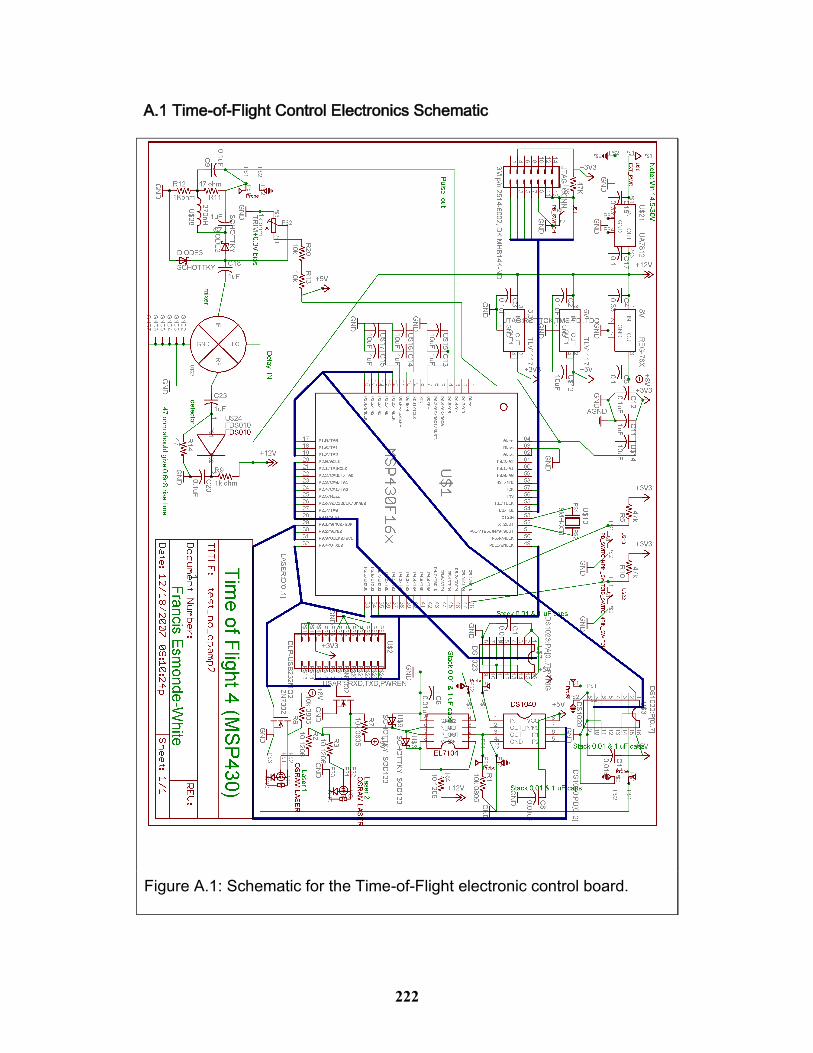
222
A.1 Time-of-Flight Control Electronics Schematic
Figure A.1: Schematic for the Time-of-Flight electronic control board.
223
A.2 Time-of-Flight Control Electronics Part List
Component [Package Type]
Voltage Regulators:
1xTLV1117-3.3 3.3 volt regulator [SOT223]
1xTLV1117-5 5 volt regulator [SOT223]
1xLM7808 8 volt regulator [SOT223]
1xUA7812 12 volt regulator [PFM-KTE]
Capacitors:
4x0.01 μF [C0603K]
7x0.1 μF [C0603K]
2x0.33 μF [C0603K]
7x1 μF [C0805K]
5x10 μF [cylindrical]
Resistors:
3x10 ohm 1206
2x47 ohm, M1206
1x1K ohm, R0603
1x1k ohm, M1206
5x10k ohm 0805
3x47K ohm, M1206
1x1k ohm variable resistor (potentiometer)
Inductor:
270 nH inductor, M0603 package
Diodes:
4 Schottky diodes [SOD-123]
Transistors:
2x2N7002 FET transistor [SOT23]
Microcontroller:
MSP430 F1611 microcontroller [PQFP64](Texas Instruments)

224
8MHz crystal oscillator [HCM49]
Integrated Circuits:
USB-to-serial converter (DLP-USB232M) (DLP Design)
DS1020 Delay line [SO16W] (Dallas Semiconductor)
DS1023 Timing element [SO16W] (Dallas Semiconductor)
DS1040 Pulse generator [SOIC8] (Dallas Semiconductor)
EL7104 Power MOSFET driver [SOIC8] (Elantec/Intersil)
MCA-12G mixer (Minicircuits)
Laser Diodes:
SPL-LL85, 850 nm pulsed laser diode
SPL-LL90, 905 nm pulsed laser diode
(OSRAM Opto Semiconductors)
Detector:
FDS010 silicon photodiode [TO5]
Mechanical Pieces and Connectors:
JTAG programming port (Digi-Key# MHB14K-ND)
0.1" spacing 2-wire screw terminal
push-button reset switch
2 bush-button switches (4 pin)
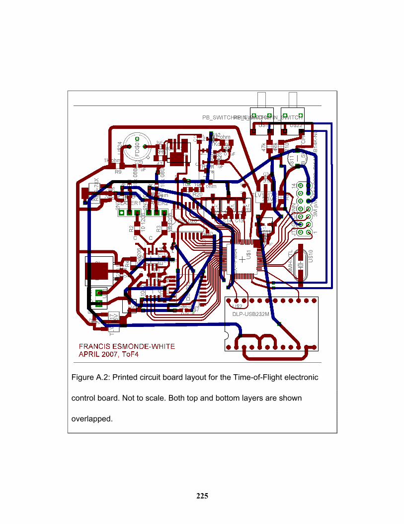
225
Figure A.2: Printed circuit board layout for the Time-of-Flight electronic
control board. Not to scale. Both top and bottom layers are shown
overlapped.
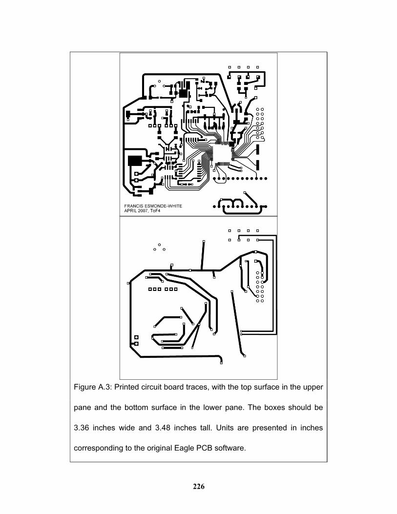
226
Figure A.3: Printed circuit board traces, with the top surface in the upper
pane and the bottom surface in the lower pane. The boxes should be
3.36 inches wide and 3.48 inches tall. Units are presented in inches
corresponding to the original Eagle PCB software.
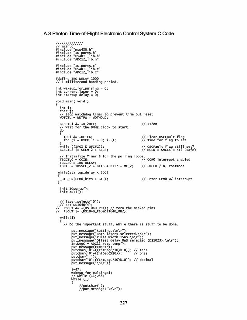
227
A.3 Photon Time-of-Flight Electronic Control System C Code
////////////// // main.c #include "msp430.h" #include "IO_ports.h" #include "USART1_lib.h" #include "ADC12_lib.h" #include "IO_ports.c" #include "USART1_lib.c" #include "ADC12_lib.c" #define IRQ_DELAY 1000 // 1 millisecond handing period. int wakeup_for_pulsing = 0; int current_laser = 0; int startup_delay = 0; void main( void ) { int i; char j; // Stop watchdog timer to prevent time out reset WDTCTL = WDTPW + WDTHOLD; BCSCTL1 &= ~XT2OFF; // XT2on // Wait for the 8MHz clock to start. do { IFG1 &= ~OFIFG; // Clear OSCFault flag for (i = 0xFF; i > 0; i--); // Time for flag to set } while ((IFG1 & OFIFG)); // OSCFault flag still set? BCSCTL2 |= SELM_2 + SELS; // MCLK = SMCLK = XT2 (safe) // Initialize Timer B for the polling loops. TBCCTL0 = CCIE; // CCR0 interrupt enabled TBCCR0 = IRQ_DELAY; TBCTL = TBSSEL_2 + BIT6 + BIT7 + MC_2; // SMCLK / 8, contmode while(startup_delay < 500) { _BIS_SR(LPM0_bits + GIE); // Enter LPM0 w/ interrupt } init_IOports(); initUART1(); // laser_select('0'); // set_DS1040(4); // P3OUT &= ~(DS1040_PB1); // zero the masked pins // P3OUT |= (DS1040_PB0&DS1040_PB2); while(1) { // Do the important stuff, while there is stuff to be done. put_message("Settings:\n\r"); put_message("Both lasers selected.\n\r"); put_message("Pulse width 15nS.\n\r"); put_message("Offset delay 0nS selected (DS1023).\n\r"); IntDegC = ADC12_read_temp(); put_message(tempstr); putchar('0'+((IntDegC/10)%10)); // tens putchar('0'+(IntDegC%10)); // ones putchar('.'); putchar('0'+((IntDegC*10)%10)); // decimal put_message("\n\r"); j=47; wakeup_for_pulsing=1; // while (++j<58) while (1) { //putchar(j); //put_message("\n\r");
228
Laser_Pulse(); ADCVal_to_ADC_resultHEX(); put_message(ADC_result); put_message("\n\r"); _BIS_SR(LPM0_bits + GIE); } wakeup_for_pulsing=0; // Enter LPM0 while waiting for stuff to do. _BIS_SR(LPM0_bits + GIE); // Enter LPM0 w/ interrupt } _BIS_SR(LPM0_bits + GIE); // Enter LPM0 w/ interrupt } // Timer B0 interrupt service routine #pragma vector=TIMERB0_VECTOR __interrupt void Timer_B (void) { TBCCR0 += IRQ_DELAY; // Add Offset to CCR0 to maintain interrupt timing. // Periodic output check if (TXCount>0) // if there is any data to be transmitted, transmit will be started. if (!(IFG2 & UTXIFG1)) //(TXBusy==0) { // Disable TX interrupt // _BIC_SR( GIE); // bit clear TXBUF1=TXBUF[TXRead++]; TXCount--; // enable TX interrupt // _BIS_SR( GIE); // bit set. } if ((~P5IN) & BUTTON_1) // check if BUTTON_1 is low. Debounce_Count_1++; else if(Debounce_Count_1>0) { if (Debounce_Count_1>=40) // was the button low for at least 40mS? { //_NOP(); // if it was, then perform the button actiond. // _BIC_SR_IRQ(LPM0_bits); // wake the uC current_laser = ( (current_laser==2)?1:2 ); // toggle between laser2 and laser1 if ( current_laser==1) laser_select('1'); else laser_select('2'); } // clear the Debounce_Count Debounce_Count_1=0; } if (startup_delay<=500) startup_delay++; else wakeup_for_pulsing=1; if (wakeup_for_pulsing) _BIC_SR_IRQ(LPM0_bits); // wake the uC // otherwise go back to sleep } ////////////// // ADC12_lib.c void ADC12init(void) { // Initialize the ADC12. P6SEL |= 0x10; // Enable A/D channel A4, pin 6.4 ADC12CTL0 &= !ENC; // DISABLE ADC12 ADC12CTL1 = SHS_0 + SHP + CONSEQ_0 + ADC12SSEL_2 + ADC12DIV_1; // Trigger Source is ADC12SC bit // SAMPCON is sourced from the sampling timer // Single-Channel, Single-Conversion // The ADC12 clock is sourced from MCLK, and divided by 2 (4MHz clock) ADC12MCTL0 = SREF_1 + INCH_4; // Channel A4, Vref+/AVss
229
ADC12CTL0 = SHT0_1 + SHT1_1 + REFON + ADC12ON; // Config ADC12 // 8 clocks for sampling, reference on at 1.5V, ADC on, ADC enabled // 2 us sampling period based on 4MHz ADC12CLK // I'm not sure about the interrupt usage ADC12IE = 0xFF; // Enable ADC12IFG.0 // I'm not triggering on Timer_A, so ignore the following 2 lines. // TACCTL1 = OUTMOD_4; // Toggle on EQU1 (TAR = 0) // TACTL = TASSEL_2 + MC_2; // SMCLK, cont-mode ADC12CTL0 |= ENC ; // Enable the ADC ADC_result[3]=0; } void ADCVal_to_ADC_resultHEX(void) { for (int i=2; i>=0; i--) { // convert from ADCval (uint, 12 bit digit) to hex (signed char[3]) ADC_result[2-i]= hextable[((ADCVal >> i*4) & 0xF)]; // ADC_result[i]= "0123456789ABCDEF"[((ADCVal >> i*4) & 0xF)]; // if hextable is unused elsewhere, then we don't use the lookup table. } } // Pulse Laser // ADC value read is stored in ADCVal, and can be extracted to hex using // ADCVal_to_ADC_resultHEX(); void Laser_Pulse(void) { // Disable Interrupts _BIC_SR( GIE); // bit clear, clear the register bits according to the bit mask. // Start the ADC12 (2uS sampling time), //Turn on and then turn off the laser line. // ADC12CTL0 &= !ENC; // DISABLE ADC12 // ADC12CTL1 = SHS_0 + SHP + CONSEQ_0 + ADC12SSEL_2 + ADC12DIV_1; // Setup ADC12 // ADC12CTL0 |= ENC ; // Enable the ADC ADC12CTL0 |= ADC12SC; // Sampling and conversion start // Turn on the Laser line // rising edge triggers the laser P3OUT = P3OUT|DS1023_PTRIG; while (!(0x01 & ADC12IFG)); // ((ADC12IFG & BIT0)==0); _NOP(); // SET BREAKPOINT HERE // while (!(0x01 & ADC12IFG)); // Conversion done? ADCVal = ADC12MEM0; // Read out 1st ADC value // Enable Interrupts _BIS_SR( GIE); // bit set, set the register bits according to the bit mask. // Turn off the laser line. This prepares for the next pulse. P3OUT = P3OUT&(~DS1023_PTRIG); return; } // read Temperature int long ADC12_read_temp(void) { _BIC_SR( GIE); ADC12CTL0 &= !ENC; // DISABLE ADC12 ADC12CTL1 = SHS_0 + SHP + CONSEQ_0 + ADC12SSEL_2 + ADC12DIV_1; // Trigger Source is ADC12SC bit, // SAMPCON is sourced from the sampling timer // Single-Channel, Single-Conversion // The ADC12 clock is sourced from MCLK, and divided by 2 (4MHz clock) ADC12MCTL0 = SREF_1 + INCH_10; // Channel A10 (temp sens), Vref+/AVss ADC12CTL0 = SHT0_7 + SHT1_7 + REFON + ADC12ON; // Config ADC12 // 128 clocks for sampling, reference on at 1.5V, ADC on, ADC enabled // 30 us sampling period based on 4MHz ADC12CLK ADC12IE = 0xFF; // Enable ADC12IFG.0 ADC12CTL0 |= ENC ; // Enable the ADC // Start the ADC12 (30uS sampling time) // Enable the ADC ADC12CTL0 |= ADC12SC; // Sampling and conversion start while (!(0x01 & ADC12IFG)); // Conversion done? (wait until done) temp = ADC12MEM0; // Read out 1st ADC value _BIS_SR( GIE);
230
IntDegC = (temp - 2692) * 423; // Calibration is probably necessary IntDegC = IntDegC / 4096; _NOP(); // << SET BREAKPOINT HERE for calibration /* while (cout_busy); // wait until cout is ready. strcopy(tempstr, str_out); // copy temp string sz_str_out = strlen(str_out); // measure string length num2str(IntDegC, tmpstr1); // convert a number to a decimal string strcopy(tmpstr1,&str_out[sz_str_out]);
// add the decimal string onto the str_out sz_str_out = strlen(str_out); // measure string length while (cout_uart0()); // wait until cout has taken the transmission string. */ // cout the temperature + ,10,13 (nl,cr) ADC12init(); // reset the ADC12 for Pulse Sampling /* ADC12CTL0 &= !ENC; // DISABLE ADC12 ADC12CTL0 = SHT0_1 + SHT1_1 + REFON + ADC12ON; // Config ADC12 // 8 clocks for sampling, reference on at 1.5V, ADC on, ADC enabled // 2 us sampling period based on 4MHz ADC12CLK ADC12MCTL0 = SREF_1 + INCH_5; // Channel A5, Vref+/AVss ADC12CTL0 |= ENC ; // Enable the ADC */ return IntDegC; } ////////////// // ADC12_lib.h unsigned int ADCVal; int long temp; int long IntDegC; char ADC_result[4]; void ADC12init(void); void ADCVal_to_ADC_resultHEX(void); void Laser_Pulse(void); int long ADC12_read_temp(void); ///////////// // IO_ports.c
void init_IOports(void) { volatile unsigned int i; volatile double j; // Set the ports for output P1DIR = 0xFF; // enable all bits in P1 as outputs P1SEL = 0x00; // set all pins as I/O P1OUT = 0x00; P2DIR = 0xFF; // enable all bits in P2 as outputs P2SEL = 0x00; // set pins as I/O P2OUT = 0x00; P3DIR |= 0x3F; // enable all non-USART bits in P3 as outputs // P3SEL = 0x00; // set pins as I/O P3OUT = 0x38; // set all pins to ground except lasers... P4DIR = 0x00; P5DIR = 0x00; // P5DIR = 0x20; // enable the P5.5 as an input // P5SEL = 0x00; // set pins as I/O // P5OUT = 0x00; // Set all pins to gnd // Set the delay to 00 set_DS1020('0','0'); // Set the delay to 00 set_DS1023('0','0'); // Ensure both lasers are on to begin. laser_select('0'); P3OUT = P3OUT&(~DS1023_PTRIG);
// set the pulse pin low so that it's ready to pulse
231
// Set DS1040 to the desired pulse (15nS) set_DS1040(4); } void set_DS1040(int i) // P5OUT = P5OUT^((P5OUT^pulse_table[4])&DS1040Mask); // Abbreviated command to swap mask-selected bits into the P5OUT pins // 100 ms power-up time. // 5 ns programming time // 0-10 ns delay { // signed int i; // volatile unsigned int tmp1, tmp2; // unsigned int setoutp=0; // i=a-'0'; if ((i<=4)&&(i>=0)) { P3OUT &= ~(0x0E); // zero the masked pins P3OUT |= pulse_table[i]; // set the proper pins on. // the pulse_table index chooses pulse length // tmp2 = P3OUT; // tmp1 = (tmp2 ^ (pulse_table[i])); // tmp1 = tmp1 & DS1040Mask; // P3OUT = ((tmp2) ^ (tmp1)); /* setoutp=~(DS1040_PB0+DS1040_PB1+DS1040_PB2); P3OUT &= setoutp; // set laser pins to 0. setoutp |= (i1&0x01)?DS1040_PB0:0x00; setoutp |= (i1&0x02)?DS1040_PB1:0x00; setoutp |= (i1&0x04)?DS1040_PB2:0x00; P3OUT |= setoutp; P3OUT &= ~setoutp; */ } } void set_DS1023_int(signed int i1) { unsigned int setoutp=0; if ((i1>=0)&&(i1<=255)) { setoutp |= (i1&0x01)?DS1023_PA0:0x00; setoutp |= (i1&0x02)?DS1023_PA1:0x00; setoutp |= (i1&0x04)?DS1023_PA2:0x00; setoutp |= (i1&0x08)?DS1023_PA3:0x00; setoutp |= (i1&0x10)?DS1023_PA4:0x00; setoutp |= (i1&0x20)?DS1023_PA5:0x00; setoutp |= (i1&0x40)?DS1023_PA6:0x00; setoutp |= (i1&0x80)?DS1023_PA7:0x00; P2OUT = setoutp; } } void set_DS1023(signed char a1, signed char a2) { signed int i1=0, i2=0; unsigned int setoutp=0; // a1 is the Low byte // a2 is the High byte if (a1!=32) // if it's a space, ignore it. { if (a1<58) i1=a1-48; else i1=a1-55; } if (a2!=32) // if it's a space, ignore it. { if (a2<58) i2=a2-48; else i2=a2-55; } i1=i1+16*i2;
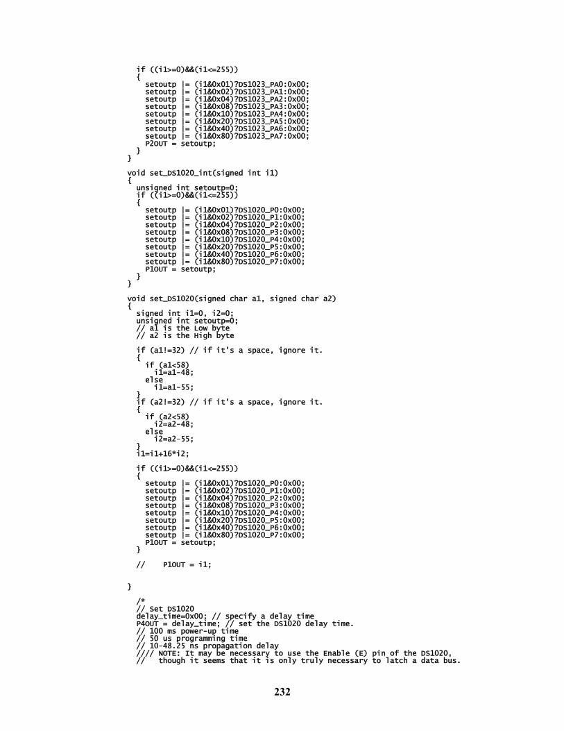
232
if ((i1>=0)&&(i1<=255)) { setoutp |= (i1&0x01)?DS1023_PA0:0x00; setoutp |= (i1&0x02)?DS1023_PA1:0x00; setoutp |= (i1&0x04)?DS1023_PA2:0x00; setoutp |= (i1&0x08)?DS1023_PA3:0x00; setoutp |= (i1&0x10)?DS1023_PA4:0x00; setoutp |= (i1&0x20)?DS1023_PA5:0x00; setoutp |= (i1&0x40)?DS1023_PA6:0x00; setoutp |= (i1&0x80)?DS1023_PA7:0x00; P2OUT = setoutp; } } void set_DS1020_int(signed int i1) { unsigned int setoutp=0; if ((i1>=0)&&(i1<=255)) { setoutp |= (i1&0x01)?DS1020_P0:0x00; setoutp |= (i1&0x02)?DS1020_P1:0x00; setoutp |= (i1&0x04)?DS1020_P2:0x00; setoutp |= (i1&0x08)?DS1020_P3:0x00; setoutp |= (i1&0x10)?DS1020_P4:0x00; setoutp |= (i1&0x20)?DS1020_P5:0x00; setoutp |= (i1&0x40)?DS1020_P6:0x00; setoutp |= (i1&0x80)?DS1020_P7:0x00; P1OUT = setoutp; } } void set_DS1020(signed char a1, signed char a2) { signed int i1=0, i2=0; unsigned int setoutp=0; // a1 is the Low byte // a2 is the High byte if (a1!=32) // if it's a space, ignore it. { if (a1<58) i1=a1-48; else i1=a1-55; } if (a2!=32) // if it's a space, ignore it. { if (a2<58) i2=a2-48; else i2=a2-55; } i1=i1+16*i2; if ((i1>=0)&&(i1<=255)) { setoutp |= (i1&0x01)?DS1020_P0:0x00; setoutp |= (i1&0x02)?DS1020_P1:0x00; setoutp |= (i1&0x04)?DS1020_P2:0x00; setoutp |= (i1&0x08)?DS1020_P3:0x00; setoutp |= (i1&0x10)?DS1020_P4:0x00; setoutp |= (i1&0x20)?DS1020_P5:0x00; setoutp |= (i1&0x40)?DS1020_P6:0x00; setoutp |= (i1&0x80)?DS1020_P7:0x00; P1OUT = setoutp; } // P1OUT = i1; } /* // Set DS1020 delay_time=0x00; // specify a delay time P4OUT = delay_time; // set the DS1020 delay time. // 100 ms power-up time // 50 us programming time // 10-48.25 ns propagation delay //// NOTE: It may be necessary to use the Enable (E) pin of the DS1020, // though it seems that it is only truly necessary to latch a data bus.
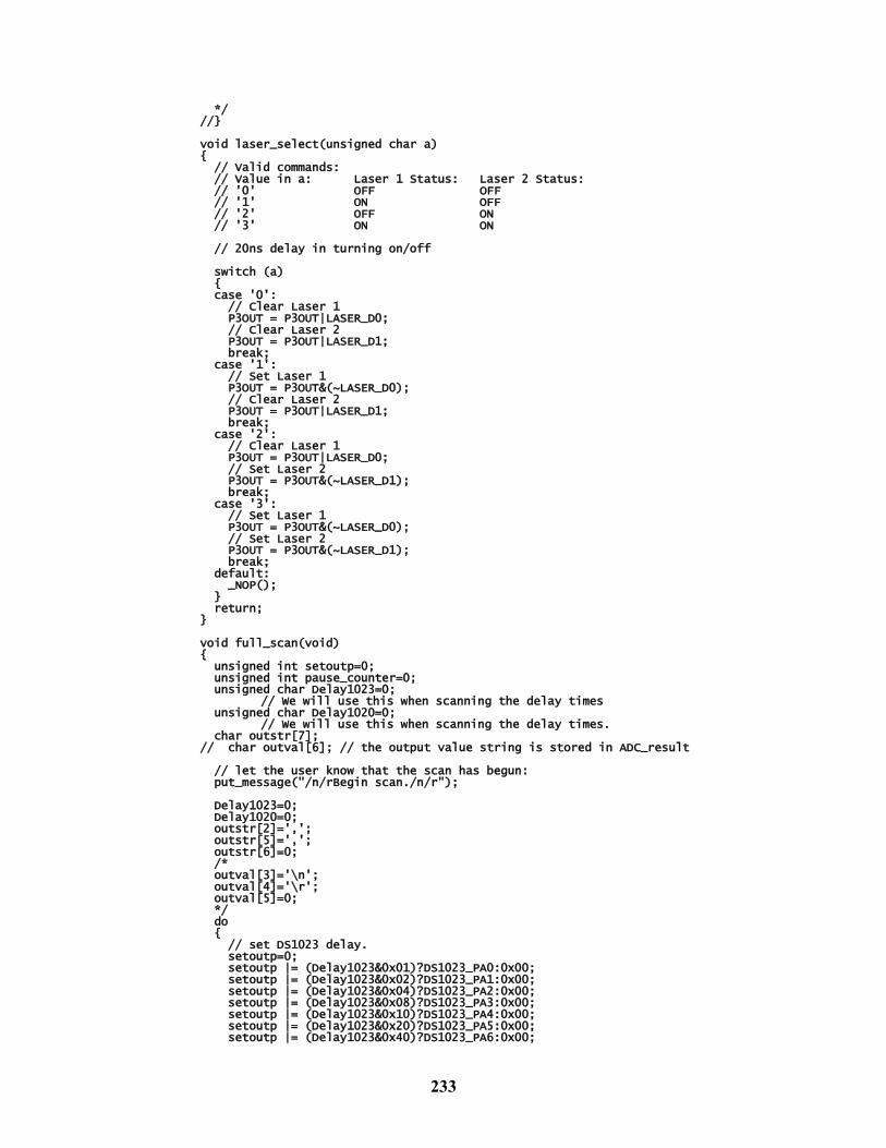
233
*/ //} void laser_select(unsigned char a) { // Valid commands: // Value in a: Laser 1 Status: Laser 2 Status: // '0' OFF OFF // '1' ON OFF // '2' OFF ON // '3' ON ON // 20ns delay in turning on/off switch (a) { case '0': // Clear Laser 1 P3OUT = P3OUT|LASER_D0; // Clear Laser 2 P3OUT = P3OUT|LASER_D1; break; case '1': // Set Laser 1 P3OUT = P3OUT&(~LASER_D0); // Clear Laser 2 P3OUT = P3OUT|LASER_D1; break; case '2': // Clear Laser 1 P3OUT = P3OUT|LASER_D0; // Set Laser 2 P3OUT = P3OUT&(~LASER_D1); break; case '3': // Set Laser 1 P3OUT = P3OUT&(~LASER_D0); // Set Laser 2 P3OUT = P3OUT&(~LASER_D1); break; default: _NOP(); } return; } void full_scan(void) { unsigned int setoutp=0; unsigned int pause_counter=0; unsigned char Delay1023=0;
// We will use this when scanning the delay times unsigned char Delay1020=0;
// We will use this when scanning the delay times. char outstr[7]; // char outval[6]; // the output value string is stored in ADC_result // let the user know that the scan has begun: put_message("/n/rBegin scan./n/r"); Delay1023=0; Delay1020=0; outstr[2]=','; outstr[5]=','; outstr[6]=0; /* outval[3]='\n'; outval[4]='\r'; outval[5]=0; */ do { // set DS1023 delay. setoutp=0; setoutp |= (Delay1023&0x01)?DS1023_PA0:0x00; setoutp |= (Delay1023&0x02)?DS1023_PA1:0x00; setoutp |= (Delay1023&0x04)?DS1023_PA2:0x00; setoutp |= (Delay1023&0x08)?DS1023_PA3:0x00; setoutp |= (Delay1023&0x10)?DS1023_PA4:0x00; setoutp |= (Delay1023&0x20)?DS1023_PA5:0x00; setoutp |= (Delay1023&0x40)?DS1023_PA6:0x00;
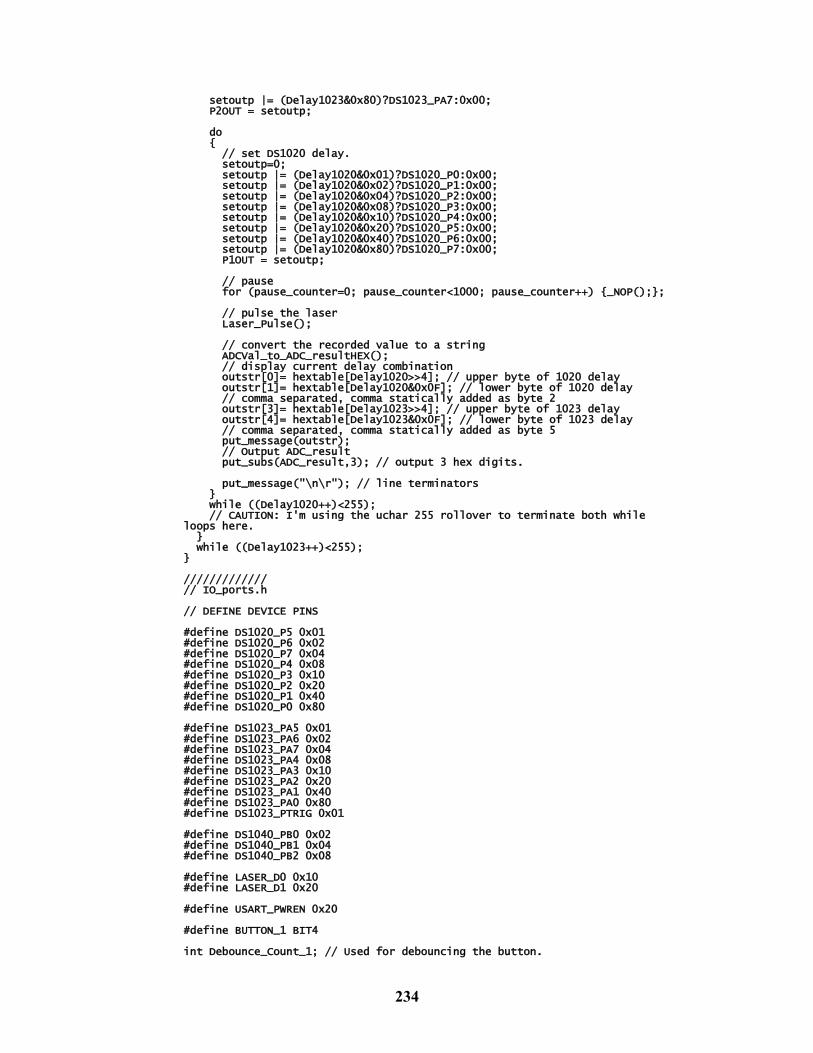
234
setoutp |= (Delay1023&0x80)?DS1023_PA7:0x00; P2OUT = setoutp; do { // set DS1020 delay. setoutp=0; setoutp |= (Delay1020&0x01)?DS1020_P0:0x00; setoutp |= (Delay1020&0x02)?DS1020_P1:0x00; setoutp |= (Delay1020&0x04)?DS1020_P2:0x00; setoutp |= (Delay1020&0x08)?DS1020_P3:0x00; setoutp |= (Delay1020&0x10)?DS1020_P4:0x00; setoutp |= (Delay1020&0x20)?DS1020_P5:0x00; setoutp |= (Delay1020&0x40)?DS1020_P6:0x00; setoutp |= (Delay1020&0x80)?DS1020_P7:0x00; P1OUT = setoutp; // pause for (pause_counter=0; pause_counter<1000; pause_counter++) {_NOP();}; // pulse the laser Laser_Pulse(); // convert the recorded value to a string ADCVal_to_ADC_resultHEX(); // display current delay combination outstr[0]= hextable[Delay1020>>4]; // upper byte of 1020 delay outstr[1]= hextable[Delay1020&0x0F]; // lower byte of 1020 delay // comma separated, comma statically added as byte 2 outstr[3]= hextable[Delay1023>>4]; // upper byte of 1023 delay outstr[4]= hextable[Delay1023&0x0F]; // lower byte of 1023 delay // comma separated, comma statically added as byte 5 put_message(outstr); // Output ADC_result put_subs(ADC_result,3); // output 3 hex digits. put_message("\n\r"); // line terminators } while ((Delay1020++)<255); // CAUTION: I'm using the uchar 255 rollover to terminate both while loops here. } while ((Delay1023++)<255); } ///////////// // IO_ports.h // DEFINE DEVICE PINS #define DS1020_P5 0x01 #define DS1020_P6 0x02 #define DS1020_P7 0x04 #define DS1020_P4 0x08 #define DS1020_P3 0x10 #define DS1020_P2 0x20 #define DS1020_P1 0x40 #define DS1020_P0 0x80 #define DS1023_PA5 0x01 #define DS1023_PA6 0x02 #define DS1023_PA7 0x04 #define DS1023_PA4 0x08 #define DS1023_PA3 0x10 #define DS1023_PA2 0x20 #define DS1023_PA1 0x40 #define DS1023_PA0 0x80 #define DS1023_PTRIG 0x01 #define DS1040_PB0 0x02 #define DS1040_PB1 0x04 #define DS1040_PB2 0x08 #define LASER_D0 0x10 #define LASER_D1 0x20 #define USART_PWREN 0x20 #define BUTTON_1 BIT4 int Debounce_Count_1; // Used for debouncing the button.
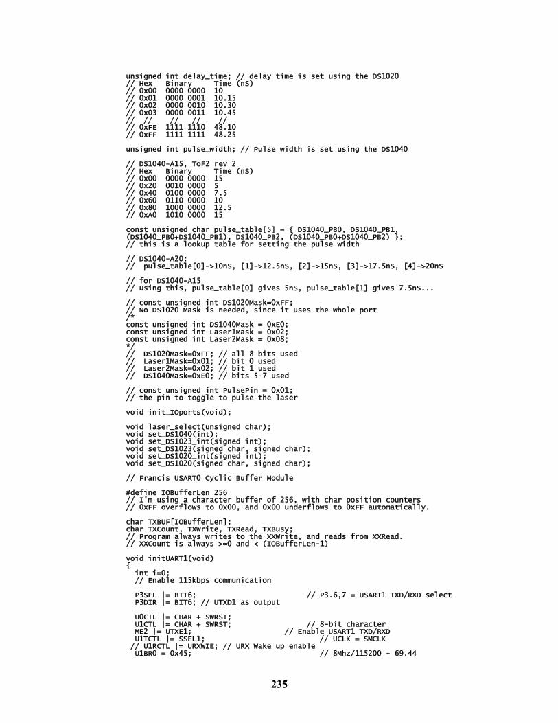
235
unsigned int delay_time; // delay time is set using the DS1020 // Hex Binary Time (nS) // 0x00 0000 0000 10 // 0x01 0000 0001 10.15 // 0x02 0000 0010 10.30 // 0x03 0000 0011 10.45 // // // // // // 0xFE 1111 1110 48.10 // 0xFF 1111 1111 48.25 unsigned int pulse_width; // Pulse width is set using the DS1040 // DS1040-A15, ToF2 rev 2 // Hex Binary Time (nS) // 0x00 0000 0000 15 // 0x20 0010 0000 5 // 0x40 0100 0000 7.5 // 0x60 0110 0000 10 // 0x80 1000 0000 12.5 // 0xA0 1010 0000 15 const unsigned char pulse_table[5] = { DS1040_PB0, DS1040_PB1, (DS1040_PB0+DS1040_PB1), DS1040_PB2, (DS1040_PB0+DS1040_PB2) }; // this is a lookup table for setting the pulse width // DS1040-A20: // pulse_table[0]->10nS, [1]->12.5nS, [2]->15nS, [3]->17.5nS, [4]->20nS // for DS1040-A15 // using this, pulse_table[0] gives 5nS, pulse_table[1] gives 7.5nS... // const unsigned int DS1020Mask=0xFF; // No DS1020 Mask is needed, since it uses the whole port /* const unsigned int DS1040Mask = 0xE0; const unsigned int Laser1Mask = 0x02; const unsigned int Laser2Mask = 0x08; */ // DS1020Mask=0xFF; // all 8 bits used // Laser1Mask=0x01; // bit 0 used // Laser2Mask=0x02; // bit 1 used // DS1040Mask=0xE0; // bits 5-7 used // const unsigned int PulsePin = 0x01; // the pin to toggle to pulse the laser void init_IOports(void); void laser_select(unsigned char); void set_DS1040(int); void set_DS1023_int(signed int); void set_DS1023(signed char, signed char); void set_DS1020_int(signed int); void set_DS1020(signed char, signed char); // Francis USART0 Cyclic Buffer Module #define IOBufferLen 256 // I'm using a character buffer of 256, with char position counters // 0xFF overflows to 0x00, and 0x00 underflows to 0xFF automatically. char TXBUF[IOBufferLen]; char TXCount, TXWrite, TXRead, TXBusy; // Program always writes to the XXWrite, and reads from XXRead. // XXCount is always >=0 and < (IOBufferLen-1) void initUART1(void) { int i=0; // Enable 115kbps communication P3SEL |= BIT6; // P3.6,7 = USART1 TXD/RXD select P3DIR |= BIT6; // UTXD1 as output U0CTL |= CHAR + SWRST; U1CTL |= CHAR + SWRST; // 8-bit character ME2 |= UTXE1; // Enable USART1 TXD/RXD U1TCTL |= SSEL1; // UCLK = SMCLK // U1RCTL |= URXWIE; // URX Wake up enable U1BR0 = 0x45; // 8Mhz/115200 - 69.44
236
U1BR1 = 0x00; // U1MCTL = 0xAA; // modulation U1CTL &= ~SWRST; // Initialize USART state machine IE2 |= UTXIE1; // Enable USART1 RX interrupt // Setup Communication Library for (i=0; i<IOBufferLen; i++) { TXBUF[i]=0; } TXCount=0; TXWrite=0; TXRead=0; TXBusy=0; /* while ( USART_PWREN & P5IN ) // Wait for DLP-USB232M windows enumeration _NOP(); */ _BIS_SR(GIE); } signed char putchar(char a) { if (TXCount<255) { // disable TX interrupt _BIC_SR( GIE); // bit clear TXBUF[TXWrite++]=a; TXCount++; // enable TX interrupt _BIS_SR( GIE); // bit set. return a; } else return -1; } static void put_subs(char *s, int sz_s) { int i=sz_s; while (i--) putchar(*s++); } static void put_message(char *s) { while (*s) putchar(*s++); } #pragma vector=USART1TX_VECTOR __interrupt void usart1_tx(void) { if (TXCount>0) { // do this if there is still data in the buffer and the TX buffer is ready. U1TXBUF=TXBUF[TXRead++]; TXCount--; } } ////////////// // USART_lib.h unsigned const char hextable[]={'0','1','2','3','4','5','6','7','8','9','A','B','C','D','E','F'}; char hellostr[]="\n\rToF 3 rev.1 Bootup Complete.\n\r\n\r\n\r"; char tempstr[]="Temp (C): "; char StrProc[80]; void initUART1(void); signed char putchar(char); static void put_subs(char*, int); static void put_message(char*);
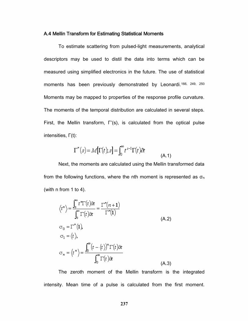
237
A.4 Mellin Transform for Estimating Statistical Moments
To estimate scattering from pulsed-light measurements, analytical
descriptors may be used to distil the data into terms which can be
measured using simplified electronics in the future. The use of statistical
moments has been previously demonstrated by Leonardi.166, 249, 250
Moments may be mapped to properties of the response profile curvature.
The moments of the temporal distribution are calculated in several steps.
First, the Mellin transform, Γ*(s), is calculated from the optical pulse
intensities, Γ(t):
(A.1)
Next, the moments are calculated using the Mellin transformed data
from the following functions, where the nth moment is represented as σn
(with n from 1 to 4).
(A.2)
(A.3)
The zeroth moment of the Mellin transform is the integrated
intensity. Mean time of a pulse is calculated from the first moment.

238
Standard deviation is calculated as the square root of the second moment.
Skew is calculated as the third moment divided by the second moment to
the power 3/2. Finally, kurtosis is calculated from the fourth moment
divided by the square of the second moment minus 3. The moments were
taken as defined by Arridge.166
239
Appendix B: Ring-Light Device
Source code for three different Matlab functions have been
included here for generating amplitude filters for making the ring patterned
lasers. Ring-patterned light is used in mathematics, physics, engineering
and chemistry. Each field uses different terminology, including: vortex
light, orbital angular momentum light, spirally phased light, and phase
singularities. Several methods for generating the ring patterns were
examined. Three such approaches are included here. In the first,
OAMmask.m, a real-valued plane phase mask is generated to emphasize
a single phase-spiral order. In the second, squareOAMmask.m, a
binarized plane phase mask is generated to produce multiple phase-spiral
orders. In the third, rotOAMmask.m, a real-valued plane phase mask is
generated in which the planar wave is incident at an angle in order to
produce a spiral phase wave normal to the filter.
function [mask]=squareOAMmask( angle, orders, masksize) % function squareOAMmask, used to make a thresholded % spiral phase function image pattern (vortex light). % % Usage: [mask]=squareOAMmask( angle, orders, masksize) where angle is
the % angle of incidence of the reference beam relative to the main planar % beam. (also the angle at which the generated OAM beam propagates)
orders % determines the number of passes used to create the square-wave pattern. % Make this a number such as 20 or 30 to see a very well thresholded % pattern. Masksize is the number of pixels for both the x and y axes. %(final mask is of size 2*masksize+1, over both x & y directions) % % Example call: % [mask]=squareOAMmask( 5, 5, [500,500]); % To generate a large binary mask.
240
% [mask]=squareOAMmask( 5, 1, [50,50]); % To generate a small fuzzy mask. % % This squareOAMmask function is derived from the following paper:
Optical % and Quantum Electronics, 24 (1992) S951-S962 Laser beams with phase % singularities, N.H. Heckenberg, R. McDuff, C.P. Smith, H. % Rubinsztein-Dunlop, and M.J. Wegener Department of Physics, the % University of Queensland, Brisbane, Australia see page S954, equation
(8) % calculate the kx for the incident reference beam, from the angle of % interference. kx=sin(pi*angle/180); % % generate a matrix of x-positions and y-positions for each pixel. xpositions=[-masksize(1):masksize(1)]'*ones(1,1+2*masksize(2)); ypositions=[[-masksize(2):masksize(2)]'*ones(1,1+2*masksize(1))]'; % determine the phase angles for each pixel relative to the center of the % Gaussian beam. [theta,r]=cart2pol(xpositions,ypositions); % % plot the phase angles figure; imagesc(theta); % % generate the OAM filter as a 2d array of intensities mask=0.5*ones(size(theta)); % % the triple-commented code is to show the mask being built, as each
new % % layer is added % % figure; % % mesh(mask) % % pause for i=1:orders; mask = mask - (sin(i*pi/2)/(i*pi/2))*cos( i*(kx*ypositions-theta) ); % If xpositions is used in the mask instead of ypositions, then the mask
is % completely different. % % mesh(mask) % % pause end % % display the OAM filter. figure; imshow(mask)
function [mask]=OAMmask( angle, masksize) % function OAMmask, generate a non-binarized vortex light holograph. % % Usage: [mask]=OAMmask( angle, masksize) % with angle being the angle of incidence for the reference beam % (and the angle at which the generated OAM beam propagates) % and masksize being used to determine the number of pixels for both the x % and y axes. % (the final mask size will be of size 2*masksize+1, over both directions) % % Example call: % [mask]=OAMmask( 5, [500,500]); % % This OAMmask function is derived from the following paper: % Optical and Quantum Electronics, 24 (1992) S951-S962 % Laser beams with phase singularities, N.H. Heckenberg, R. McDuff, % C.P. Smith, H. Rubinsztein-Dunlop, and M.J. Wegener % Department of Physics, the University of Queensland, Brisbane, Australia % see page S954, equation (5) % % calculate the kx for the incident reference beam, based on the angle of interference. kx=sin(pi*angle/180);
241
% % generate a matrix of x-positions and y-positions for each pixel. xpositions=[-masksize(1):masksize(1)]'*ones(1,1+2*masksize(2)); ypositions=[[-masksize(2):masksize(2)]'*ones(1,1+2*masksize(1))]'; % % determine the phase angles for each pixel relative to the center of the % % Gaussian beam. [theta,r]=cart2pol(xpositions,ypositions); % % plot the phase angles % figure; imagesc(theta); % % generate the OAM filter as a 2d array of intensities mask = 0.5*(1-cos(kx*xpositions-theta)); % % If xpositions is used in the mask instead of ypositions, then the mask is % % completely different. % % display the OAM filter. figure; imshow(mask)
function [mask]=rotOAMmask( omega, masksize, wavenum) % function rotOAMmask, to generate OAM beams from a plane wave incident at % an angle omega from the filter normal, such that the final annular/vortex % beam propagates normal to the filter rather than at an angle. % % Usage: [mask]=rotOAMmask( angle, masksize, wavelength) with angle being % the angle of incidence for the reference beam % (and the angle at which the generated OAM beam propagates) % and masksize being used to determine the number of pixels for both the x % and y axes. % (the final mask size will be of size 2*masksize+1, over both % directions) % % Example usage: % [mask]=rotOAMmask( 30, [1000, 1000], 650); % % This OAMmask function is derived from the following paper: Optical and % Quantum Electronics, 24 (1992) S951-S962 Laser beams with phase % singularities, N.H. Heckenberg, R. McDuff, C.P. Smith, H. % Rubinsztein-Dunlop, and M.J. Wegener Department of Physics, the % University of Queensland, Brisbane, Australia see page S954, equation (5) % Additional modifications by Francis Esmonde-White to rotate the computed % filter plane. % % calculate the kx for the incident reference beam, based on the angle of % interference. kx=sin(pi*omega/180); % % generate a matrix of x-positions and y-positions for each pixel. xpositions=[-masksize(1):masksize(1)]'*ones(1,1+2*masksize(2)); ypositions=[[-masksize(2):masksize(2)]'*ones(1,1+2*masksize(1))]'; % the interference plane zpositions=xpositions*kx; xpositions=xpositions*cos(pi*omega/180);

242
% % determine the phase angles for each pixel relative to the center of the % % Gaussian beam. [theta,r]=cart2pol(xpositions,ypositions); % figure; imagesc(theta) % the plane wave has intensity 1 everywhere mask=0.5*(1-cos(3/2*pi-theta+2*pi*zpositions/wavenum)); % for each theta, we need to add the change due to the difference in the z % plane position (which z=0 has become z*cos(theta)+x*sin(theta)=0) % % plot the phase angles figure; imagesc(theta); % % generate the OAM filter as a 2d array of intensities mask = % 0.5*(1-cos(kx*xpositions-theta)); % If xpositions is used in the mask % instead of ypositions, then the mask is % completely different. % display the OAM filter. figure; imshow(mask)
243
Appendix C: Genetic Algorithm Code
function thesis_GA(savefile) warning off % Thesis GA % load lactate data % wlrange=find((wave>=1500)&(wave<=1750)); load lactate numtot=10; % ten samples total numval=1; % choose 4 validation samples numspec=4; % 4 spectra per sample numwl=size(data,2); % 987 wavelengths sampleset=1:numspec:numtot*numspec; comb=nchoosek(sampleset,numval); % permutation combinations pop_sz=200; % 200 population members N=6; % maximum possible number of pre-processing steps. % Size information for the genetic bitstring representation of models numbits_preproc=N*14; % number of bits required for the pre-processing
option numbits_HT=2^ceil(log2(numwl)); % number of bits required for Haar
transform selection numbits=numbits_preproc+numwl+numbits_HT; % total number of bits required GA_iter_max=pop_sz*50; % number of evolution iterations saveinterval=50; % interval (in evolution steps) at which to save the
results maxmodelsz=numtot*numspec; % choose a maximum number of wavelengths to
allow in a solution % initialize matrix sizes bestmodels=false(maxmodelsz,N+1,numbits); % store the best population
members bestmodelsres=NaN(maxmodelsz,N+1); % store indeces to results for the
best members bestmodelfit=NaN(maxmodelsz,N+1); % fitness values of the best members modelcount=zeros(maxmodelsz,N+1); % number of models built in each
category popfitness=zeros(1,pop_sz); % vector of population fitnesses popres=zeros(1,pop_sz); % indeces pointing to results for each of the
current population members % randomly generate an initial GA population % total number of bits: % pre-processing options + wavelength selection + FWT component selection % N*14+numwl+ (1:(2^ceil(log2(numwl)))) pop=[(rand(pop_sz,numbits_preproc)<0.5),
(rand(pop_sz,numwl)<((numtot*numspec)/(5*numwl))), (rand(pop_sz,numbits_HT)<((numtot*numspec)/(5*numbits_HT)))];
init_mut_rate=0.10; % initial mutation rate mut_rate=0.10; % 10% mutation rate % big matrix in which to store results for all evaluate strings % (indexed by popres and bestmodelsres) result=zeros(GA_iter_max,10); % begin the GA for GA_iter=1:GA_iter_max disp(['Iteration: ',num2str(GA_iter)]) % let the user know how things
are progressing if mod(GA_iter,saveinterval)==0 % periodically save based on the
selected interval
244
save(savefile) % the savefile is selected in the GA function call.
mut_rate=mut_rate+0.004; % increase the mutation rate as the evolution progresses
end % select the genetic vector to evaluate for fitness (by copying to
"bitstring") if GA_iter<=pop_sz % Fitnesses of the randomly initialized
population are first % evaluated. By taking the vector from the population at the
current index. bitstring=pop(GA_iter,:); else % Make a new vector from the existing population and process it. [popfitness,popind]=sort(popfitness,'ascend'); % sort the
population according to fitness % This depends on the type of fitness value used. (examples in
brackets) % Ascending fitness sorting will leave small values at the top.
(residual, cost) % Descending fitness sorting will leave big values at the top.
(linearity, probability) % popfitness=popfitness(1:ev_pop_size); % Already sorted pop=pop(popind,:); % sort the population members according to the
fitness popres=popres(popind); % keep the results vector correctly
indexed % FITNESS ORDERING/SCALING scaled_fitnesses = cumsum(1./popfitness); % scale the fitnesses between zero and one % minfit = min(scaled_fitnesses); maxfit = max(scaled_fitnesses); % scaled_fitnesses = (scaled_fitnesses-minfit)/(maxfit-
minfit+eps); scaled_fitnesses = (scaled_fitnesses)/(maxfit+eps); % find the first parent based on the scaled fitness parent1 = find(scaled_fitnesses<=rand(1),1,'last'); if isempty(parent1) % if no first parent is selected yet parent1=1; end % crossover & mutation mut = rand(1)<mut_rate; % mutation? if (mut) % if performing a mutation evolution step mut_count=ceil(5*abs(randn(1)).^1.5); % number of mutations % distribution of mutation counts so there are some rare % mutations of many bits and many mut's with few bits bits_to_mutate=1+ceil(rand(1,mut_count)*(numbits-1));% bit
positions to mutate % perform the mutation bitstring = pop(parent1,:); % copy the original vector bitstring(bits_to_mutate)=~bitstring(bits_to_mutate); %
invert the selected bits else % if performing a crossover evolution step n_cx=ceil((rand(1)^3)*4); % initial number of crossover
points cx_ind=unique(1+ceil(rand(1,n_cx)*(numbits-1))); % choose the
crossover points n_cx=numel(cx_ind); % count of unique crossover steps % find the second parent based on the scaled fitness parent2 = find(scaled_fitnesses<=rand(1),1,'last');
245
% index of the second parent selected (the first is selected above)
% Error checking if isempty(parent2) % if no second parent is selected yet parent2=2; % default second parent. end % if the same parent is selected for both parents if parent1==parent2; parent2=mod(parent1+1,pop_sz-1)+1; % select a different
second parent end % Perform the crossover % at least one crossover point must be present bitstring =
[pop(parent1,1:cx_ind(1)),pop(parent2,(cx_ind(1)+1):end)]; if (n_cx>=2) % if two cx points, then add next segment. bitstring((cx_ind(2)+1):end) =
pop(parent1,(cx_ind(2)+1):end); if (n_cx>=3) % if 3 cx points, then add next segment. bitstring((cx_ind(3)+1):end) =
pop(parent2,(cx_ind(3)+1):end); if (n_cx==4) % if 4 cx points, then add next segment. bitstring((cx_ind(4)+1):end) =
pop(parent1,(cx_ind(4)+1):end); end end end end end % initialize result vectors for the permutation fitness evaluation ctrue=[]; % known calibration concentrations cest=[]; % estimated calibration concentrations vtrue=[]; % known validation concentrations vest=[]; % estimated validation concentrations sens=[]; % sensitivity from each calibration tic; % start the timer for permut=1:size(comb,1); % choose the permutation iteration % process all permutations of the data using the model bitstring. % initialize the temporary calibration and validation data cal=zeros((numtot-numval)*numspec,987); % calibration spectra cal_known=zeros(1,(numtot-numval)*numspec); % calibration
reference values val=zeros(numval*numspec,987); % validation spectra val_known=zeros(1,numval*numspec); % validation reference values % select data for calibration (not already selected for
validation) comb_compl=setdiff(sampleset,comb(permut,:)); % comb is initialized at the beginning of the function, and % contains the nchoosek() permutation orderings for i=1:(numtot-numval); % r and r2 just get the correct indeces r=(1:numspec)+numspec*(i-1); r2=(1:numspec)+comb_compl(i)-1; cal(r,:)=data(r2,:); % select the calibration data cal_known(r)=known(r2); % select the calibration reference
values end % copy the validation data into the temporary matrices for i=1:numval; r=(1:4)+4*(i-1); r2=(1:4)+comb(permut,i)-1; val(r,:)=data(r2,:); % select the validation data val_known(r)=known(r2); % select the validation reference
values
246
end % Evaluate the fitness of the current bitstring
[tmp,ce,ck,ve,vk]=GA_processing(cal,cal_known,val,val_known,bitstring,numwl,N);
% store the temporary results ctrue=[ctrue,ck]; cest=[cest,ce]; vtrue=[vtrue,vk]; vest=[vest,ve]; sens=[sens,tmp(5)]; end % check that the fitness function returned the right number of total % values (when the model fails, it will not return consistent
numbers) if (numel(ctrue)==numel(cest))&(tmp(6)<numel(vtrue)) % MSE(Mean Square Error) % from: % Probability and Statistics for engineering and the sciences, % Jay L. Devore, Sixth Edition. Brooks/Cole - Thomson learning.
2004 % Chapter 13 (13.4 in particular) % n is the number of y-values or equations. n(1)=numel(ctrue); % n for calibration n(2)=numel(vtrue); % n for validation % This is where PARSIMONY is applied. Either define MSE as: % % No parsimony % SSE/(n) for no parsimony % % Parsimony with # wavelengths % SSE/(n-(k+1)) where k is # of wavelengths for parsimony by WL % % Parsimony with # wavelengths & # pre-processing options % SSE/(n-(k+1)) where k is # of wl & # of pre-processing options k=tmp(6); % k is the number of wavelengths used in the model % Use the following line for WL & PP option penalty k=k+tmp(7); % k is now additionally penalized for the number of
pp options used in the model SST(1)=sum(ctrue.^2)-(sum(ctrue)^2)/n(1); SSE(1)=sum((cest-ctrue).^2); SST(2)=sum(vtrue.^2)-(sum(vtrue)^2)/n(2); SSE(2)=sum((vest-vtrue).^2); MSE(1)=SSE(1)/(n(1)-(k+1)); % p. 594 of Devore's book MSE(2)=SSE(2)/(n(2)-(k+1)); result(1)=MSE(1); result(2)=MSE(2); R2(1)=1-SSE(1)/SST(1); R2(2)=1-SSE(2)/SST(2); R2adj(1)=((n(1)-1)*R2(1)-k)/(n(1)-(k+1)); R2adj(2)=((n(2)-1)*R2(2)-k)/(n(2)-(k+1)); result(GA_iter,1)=MSE(1); result(GA_iter,2)=MSE(2); result(GA_iter,3)=R2adj(1); result(GA_iter,4)=R2adj(2); % Non-parsimony penalized results for storage & later comparison. result(GA_iter,9)=sqrt(sum((ctrue-cest).^2)/numel(ctrue)); % RMSE
247
result(GA_iter,10)=sqrt(sum((vtrue-vest).^2)/numel(vtrue)); % RMSE
% Alternate measure (RMSE, MSE, or SDEP are equivalent) % result(GA_iter,1)=sqrt(sum((ctrue-cest).^2)/numel(ctrue)); % result(GA_iter,2)=sqrt(sum((vtrue-vest).^2)/numel(vtrue)); % % Corresponds to SDEP of R. Todescini et al., p. 160, Nature % % inspired methods in chemometrics:... (2003 Leardi book) else % if invalid model, result is set to not-a-number result(GA_iter,1:4)=NaN; end % store model details in the results matrix result(GA_iter,5)=mean(sens); % mean sensitivity result(GA_iter,6)=tmp(6); % store # wavelengths selected result(GA_iter,7)=tmp(7); % store # pre-processing options selected result(GA_iter,8)=toc; % store total processing time % Display model processing time (allows a rough estimate of the % required time for a complete algorithm run. disp([' Mean/total model processing time: ',
num2str([result(GA_iter,8)/permut,result(GA_iter,8)])]); % determine the statistical properties of the model. if (result(GA_iter,6)>0)&~sum(isnan(result(GA_iter,:)));
% if the model is properly evaluated % select the fitness property to use: this allows different
results to be chosen. str_fitness=result(GA_iter,2); % MSE adjusted for model size else % otherwise the model fitness is set to not-a-number str_fitness=NaN; end % if the new model is succesfully evaluated and has suitably good
fitness, % and there is no current best model or the model is better than the
current best model... then % store it for later comparison in the 'bestmodels' arrays. tmp_wlcount=result(GA_iter,6); tmp_ppcount=result(GA_iter,7); if ~isnan(str_fitness)&(tmp_wlcount<=maxmodelsz)
modelcount(tmp_wlcount,tmp_ppcount+1)=modelcount(tmp_wlcount,tmp_ppcount+1)+1;
if isnan(bestmodelfit(tmp_wlcount,tmp_ppcount+1))|(str_fitness<bestmodelfit(tmp_wlcount,tmp_ppcount+1))
bestmodels(tmp_wlcount,tmp_ppcount+1,:)=bitstring; bestmodelsres(tmp_wlcount,tmp_ppcount+1)=GA_iter; bestmodelfit(tmp_wlcount,tmp_ppcount+1)=str_fitness; end end if GA_iter<=pop_sz % if evaluating the population for the first time,
then store all the results popfitness(GA_iter)=str_fitness; popres(GA_iter)=GA_iter; else % if evaluating evolution members, then compare & replace a
suitable member. % either replace the first parent, or the last bitstring in the % population, depending if the new bitstring is better than the % parent1 or the pop(end) members. if ~isnan(str_fitness) if
isnan(popfitness(parent1))|(str_fitness<=popfitness(parent1)) % Replace the first parent popfitness(parent1)=str_fitness; pop(parent1,:)=bitstring; popres(parent1)=GA_iter;
248
else % replace the first unsuccesful member of the population % (where fitness is 'NaN') ind=find(isnan(popfitness),1,'first'); if (~isempty(ind)) % if there is a NaN member, replace
it. popfitness(ind)=str_fitness; pop(ind,:)=bitstring; popres(ind)=GA_iter; else % otherwise find the last member with lower fitness ind=find(popfitness>=str_fitness,1,'last'); if (~isempty(ind)) % if there is a lower member,
replace it. popfitness(ind)=str_fitness; pop(ind,:)=bitstring; popres(ind)=GA_iter; else % if none of these is replaced, then keep the
member anyways % replace one of the 20% worst members anyways % (serves to keep some randomized members &
maintain genetic diversity) ind=ceil((.8+rand(1)/5)*pop_sz); popfitness(ind)=str_fitness; pop(ind,:)=bitstring; popres(ind)=GA_iter; end end end end end end warning on %%%%%% Support Functions %%%%%% %%%%%%%%%%%%%%%%%%%%%%%%%%%%%%% %%%%% Function graytoreal function realval=graytoreal(bitstring) % convert the gray coded bitstring into a real value and return as
realval binstr = bitstring; % convert gray code to binary for k=2:numel(bitstring) if (binstr(k-1)) binstr(k)= ~binstr(k); end end % convert the binary string to a real value realval = polyval(binstr, 2); %%%%% Function second_deriv function [modeldata, testdata] = second_deriv(modeldata, testdata,
window, gap, v) % Second derivative function window=2*round((window-0.1)/2)+1; % an odd integer gap=2*round((gap-0.1)/2)+1; % an odd integer gapderiv=zeros(1,gap); gapderiv((gap-1)/2)=-2; gapderiv([1,end])=1; filter=conv(conv(ones(1,window),ones(1,window)),gapderiv/gap); ends = (numel(filter)-1)/2; modeldata=conv2(modeldata,filter); cutoff1 = round((size(modeldata,2)-v)/2); cutoff2 = size(modeldata,2)-v-cutoff1;
249
modeldata(:,[1:cutoff1, (end-cutoff2+1):end])=[]; modeldata(:,1:ends)=repmat(modeldata(:,ends+1),[1,ends]); modeldata(:,(end-ends+1):end)=repmat(modeldata(:,end-ends),[1,ends]); testdata=conv2(testdata,filter); testdata(:,[1:cutoff1, (end-cutoff2+1):end])=[]; testdata(:,1:ends)=repmat(testdata(:,ends+1),[1,ends]); testdata(:,(end-ends+1):end)=repmat(testdata(:,end-ends),[1,ends]); %%%%% Function first_deriv function [modeldata, testdata] = first_deriv(modeldata, testdata, window,
gap, v) % First Derivative function window=2*round((window-0.1)/2)+1; % an odd integer gap=2*round((gap-0.1)/2)+1; % an odd integer % double smooth gapderiv=zeros(1,gap); gapderiv(1)=1; gapderiv(end)=-1; filter=conv(conv(ones(1,window),ones(1,window)),gapderiv/gap); ends = (numel(filter)-1)/2; modeldata=conv2(modeldata,filter); cutoff1 = round((size(modeldata,2)-v)/2); cutoff2 = size(modeldata,2)-v-cutoff1; modeldata(:,[1:cutoff1, (end-cutoff2+1):end])=[]; modeldata(:,1:ends)=repmat(modeldata(:,ends+1),[1,ends]); modeldata(:,(end-ends+1):end)=repmat(modeldata(:,end-ends),[1,ends]); testdata=conv2(testdata,filter); testdata(:,[1:cutoff1, (end-cutoff2+1):end])=[]; testdata(:,1:ends)=repmat(testdata(:,ends+1),[1,ends]); testdata(:,(end-ends+1):end)=repmat(testdata(:,end-ends),[1,ends]); %%%%% Function haar1d function Dout=haar1d(Din) % Take the 1D Haar Transform along the second dimension: % based on http://www.cs.ucf.edu/~mali/haar/ % % The algorithm pads the data with the last datapoint in each vector to a % length of 2^ceil(log2(size(data,2))). % % Usage: Dout=haar1d(Din); % % Francis Esmonde-White, July 2007 n=2^ceil(log2(size(Din,2))); w=n; [sz1,sz2]=size(Din); Dout=zeros(sz1,n); % D=zeros(1,n); D=repmat(Din(:,end),[1,n]); D(:,1:sz2)=Din; sqrt2=sqrt(2); while (w>1); w=w/2; for i=0:(w-1); Dout(:,i+1)=(D(:,2*i+1)+D(:,2*i+2))/sqrt2; Dout(:,i+w+1)=(D(:,2*i+1)-D(:,2*i+2))/sqrt2; end for i=1:(w*2) D(:,i)=Dout(:,i); end end %%%%% Function GA_processing (regression fitness function)
250
function [result,cal_est,cal_known,val_est,val_known] = GA_processing(cal,cal_known,val,val_known,bitstring,numwl,N)
% GA_processing function % % Takes the calibration and validation data, along with the known % assignments, and estimates the fitness of the model specified by % bitstring. % % numwl is the number of wavelengths. % N is the number of pre-processing options. % % The output is a vector 'result' that contains the desired model % performance information. is_HWT = false; % by default we assume that we do not use the HWT is_badmodel = false; % by default we assume that the model is good result=zeros(1,5); % initialize the result array opt_count=0; % initialize the count of pre-processing options to use % initialize the calibration and validation estimate vectors cal_est=NaN; val_est=NaN; % First we check to ensure that the current model has some wavelengths
selected! for preproc_N=1:N; % iterate through the pre-processing options Pbits=bitstring((1:14)+(preproc_N-1)*14); % select the relevant pre-
processing option string Pvals(1)=graytoreal(Pbits(1:4)); % convert the pre-processing string
to a real value if (Pvals(1)>=1)&(Pvals(1)<=12) % Does the selected option value
specify a pre-processing step? opt_count=opt_count+1; end % is the haar transform option selected? if (Pvals(1)==12) % FWT is_HWT=true; end end % we need to check to ensure that some parameters are used in the
regression. if is_HWT % ensure that at least one HWT parameter is selected for regression if (sum(bitstring(N*14+(1:numwl)))==0) % model has no selected wavelengths is_badmodel=true; end else if sum(bitstring(N*14+numwl+ (1:(2^ceil(log2(numwl))))))==0 % model has no selected wavelengths is_badmodel=true; end end % if the model doesn't use any wavelengths, it's a bad model and should
be skipped. if is_badmodel result(1:7)=NaN; return; end for preproc_N=1:N; % For each pre-processing option % First chop the bitstring into a series of Pbits, for each allowed
option Pbits=bitstring((1:14)+(preproc_N-1)*14); % preproc_N specifies the
index of the current pre-processing option
251
% Next decode Pbits into Pvals % Pbits is stored as Grey code, and must be decoded to real values. % Pvals(1) is the selected technique, between 0 and 15 % 4 bits Pvals(1)=graytoreal(Pbits(1:4)); % Pvals(2) selects wavelength axis (0) or sample axis (1) % 1 bit Pvals(2)=Pbits(5); % Pvals(3) specifies smoothing window, an integer between 1 and 32. % 5 bits Pvals(3)=graytoreal(Pbits(6:10))+1; % Pvals(4) specifies derivative gap, an odd integer between 3 and 34. % 4 bits Pvals(4)=2*graytoreal(Pbits(11:14))+3; % Allow N spaces for pre-processing to enable that many options and
allow % them to self-order. switch Pvals(1) case 0 % do nothing, the option is disabled. case 1 % mean centering % Pvals(2)==0 by wavelength if (Pvals(2)==0) val=val-repmat(mean(cal),[size(val,1),1]); cal=cal-repmat(mean(cal),[size(cal,1),1]); % Pvals(2)==1 by sample elseif (Pvals(2)==1) val=val-repmat(mean(val,2),[1,size(val,2)]); cal=cal-repmat(mean(cal,2),[1,size(cal,2)]); end case 2 % autoscaling % Pvals(2)==0 by wavelength % mean center by wavelength and scale by wavelength
variance if (Pvals(2)==0) val=val-repmat(mean(cal),[size(val,1),1]); cal=cal-repmat(mean(cal),[size(cal,1),1]); val=val./repmat(std(cal),[size(val,1),1]); cal=cal./repmat(std(cal),[size(cal,1),1]); % Pvals(2)==1 by sample % mean center by sample and scale by sample variance elseif (Pvals(2)==1) val=val-repmat(mean(val,2),[1,size(val,2)]); cal=cal-repmat(mean(cal,2),[1,size(cal,2)]); val=val./repmat(std(val,0,2),[1,size(val,2)]); cal=cal./repmat(std(cal,0,2),[1,size(cal,2)]); end case 3 % scale to variance % Pvals(2)==0 per wavelength if (Pvals(2)==0) val=val./repmat(std(cal),[size(val,1),1]); cal=cal./repmat(std(cal),[size(cal,1),1]); % Pvals(2)==1 per sample elseif (Pvals(2)==1) val=val./repmat(std(val,0,2),[1,size(val,2)]); cal=cal./repmat(std(cal,0,2),[1,size(cal,2)]); end case 4 % scale range to 0-1 % Pvals(2)==0 per wavelength if (Pvals(2)==0) minc=min(cal); rangec=max(cal)-minc; val=(val-
repmat(minc,[size(val,1),1]))./repmat(rangec,[size(val,1),1]);
252
cal=(cal-repmat(minc,[size(cal,1),1]))./repmat(rangec,[size(cal,1),1]);
% Pvals(2)==1 per sample elseif (Pvals(2)==1) minc=min(val,[],2); rangec=max(val,[],2)-minc; val=(val-
repmat(minc,[1,size(val,2)]))./repmat(rangec,[1,size(val,2)]); minc=min(cal,[],2); rangec=max(cal,[],2)-minc; cal=(cal-
repmat(minc,[1,size(cal,2)]))./repmat(rangec,[1,size(cal,2)]); end case 5 % scale to max 1 % Pvals(2)==0 per wavelength if (Pvals(2)==0) rangec=max(cal); val=val./repmat(rangec,[size(val,1),1]); cal=cal./repmat(rangec,[size(cal,1),1]); % Pvals(2)==1 per sample elseif (Pvals(2)==1) rangec=max(val,[],2); val=val./repmat(rangec,[1,size(val,2)]); rangec=max(cal,[],2); cal=cal./repmat(rangec,[1,size(cal,2)]); end case 6 % normalize to area 1 % Pvals(2)==0 per wavelength if (Pvals(2)==0) rangec=sum(cal); val=val./repmat(rangec,[size(val,1),1]); cal=cal./repmat(rangec,[size(cal,1),1]); % Pvals(2)==1 per sample elseif (Pvals(2)==1) rangec=sum(val,2); val=val./repmat(rangec,[1,size(val,2)]); rangec=sum(cal,2); cal=cal./repmat(rangec,[1,size(cal,2)]); end case 7 % normalize to norm 1 % Pvals(2)==0 per wavelength if (Pvals(2)==0) normc=zeros(1,size(cal,2)); for i=1:size(cal,2); normc(i)=norm(cal(:,i)); end val=val./repmat(normc,[size(val,1),1]); cal=cal./repmat(normc,[size(cal,1),1]); % Pvals(2)==1 per sample elseif (Pvals(2)==1) normc=zeros(size(val,1),1); for i=1:size(val,1); normc(i)=norm(val(i,:)); end val=val./repmat(normc,[1,size(val,2)]); normc=zeros(size(cal,1),1); for i=1:size(cal,1); normc(i)=norm(cal(i,:)); end cal=cal./repmat(normc,[1,size(cal,2)]);
253
end case 8 % linear detrend by sample val=detrend(val')'; cal=detrend(cal')'; case 9 % smoothing along sample % Pvals(3) specifies smoothing window sm=2*Pvals(3)+1; % calculate the smoothing window tmp=conv2(val,ones(1,sm)); % smooth the data val=tmp(:,(1+Pvals(3)):(end-Pvals(3))); % chop the ends off val(:,1:Pvals(3))=repmat(val(:,Pvals(3)+1),[1,Pvals(3)]); %
adjust the first end val(:,(end-Pvals(3)+1):end)=repmat(val(:,end-
Pvals(3)),[1,Pvals(3)]); % adjust the second end tmp=conv2(cal,ones(1,sm)); cal=tmp(:,(1+Pvals(3)):(end-Pvals(3))); cal(:,1:Pvals(3))=repmat(cal(:,Pvals(3)+1),[1,Pvals(3)]); cal(:,(end-Pvals(3)+1):end)=repmat(cal(:,end-
Pvals(3)),[1,Pvals(3)]); % intrinsic smoothing function sometimes stalls in infinite
loops % for i=1:size(val,1); % val(i,:)=smooth(val(i,:),Pvals(3)); % end % for i=1:size(cal,1); % cal(i,:)=smooth(cal(i,:),Pvals(3)); % end case 10 % first deriv along sample % Pvals(3) specifies smoothing window % Pvals(4) specifies derivative gap sm=2*(Pvals(3)-1)+1; [cal, val] = first_deriv(cal, val, sm, Pvals(4),
size(cal,2)); % v is the original number of wavelengths case 11 % second deriv along sample % Pvals(3) specifies smoothing window % Pvals(4) specifies derivative gap sm=2*(Pvals(3)-1)+1; [cal, val] = second_deriv(cal, val, sm, Pvals(4),
size(cal,2)); case 12 % FWT is_HWT=true; cal=haar1d(cal); val=haar1d(val); % case 13 % NO SVD IMPLEMENTED YET % % SVD otherwise % do nothing end end if (is_HWT) wlstring=bitstring(N*14+numwl+ (1:(2^ceil(log2(numwl))))); % determine the activated FWT components from the selected % wavelengths. selwl=find(wlstring); beta=cal_known/[ones(size(cal,1),1),cal(:,selwl)]'; cal_est=beta*[ones(size(cal,1),1),cal(:,selwl)]'; val_est=beta*[ones(size(val,1),1),val(:,selwl)]';
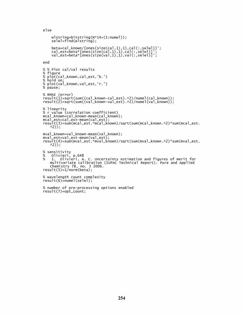
254
else wlstring=bitstring(N*14+(1:numwl)); selwl=find(wlstring); beta=cal_known/[ones(size(cal,1),1),cal(:,selwl)]'; cal_est=beta*[ones(size(cal,1),1),cal(:,selwl)]'; val_est=beta*[ones(size(val,1),1),val(:,selwl)]'; end % % Plot cal/val results % figure % plot(cal_known,cal_est,'b.') % hold on; % plot(val_known,val_est,'r.') % pause; % RMSE (error) result(1)=sqrt(sum((cal_known-cal_est).^2)/numel(cal_known)); result(2)=sqrt(sum((val_known-val_est).^2)/numel(val_known)); % linearity % r value (correlation coefficient) mcal_known=cal_known-mean(cal_known); mcal_est=cal_est-mean(cal_est); result(3)=sum(mcal_est.*mcal_known)/sqrt(sum(mcal_known.^2)*sum(mcal_est.
^2)); mval_known=val_known-mean(val_known); mval_est=val_est-mean(val_est); result(4)=sum(mval_est.*mval_known)/sqrt(sum(mval_known.^2)*sum(mval_est.
^2)); % sensitivity % Olivieri, p.648 % 1. Olivieri, A. C. Uncertainty estimation and figures of merit for
multivariate calibration (IUPAC Technical Report). Pure and Applied Chemistry 78, no. 3 2006.
result(5)=1/norm(beta); % wavelength count complexity result(6)=numel(selwl); % number of pre-processing options enabled result(7)=opt_count;
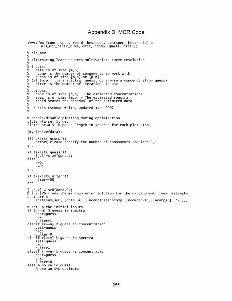
255
Appendix D: MCR Code
function [conc, spec, resid, bestconc, bestspec, bestresid] = als_mcr_deriv_clos( data, ncomp, guess, niter);
% als_mcr % % Alternating least squares multivariate curve resolution % % inputs: % data is of size [m,n] % ncomp is the number of components to work with % guess is of size [m,p] or [p,n] % (if [m,p] it's a spectral guess, otherwise a concenctration guess) % niter is the number of iterations to use % % outputs: % conc is of size [p,n] - The estimated concentrations % spec is of size [m,p] - The estimated spectra % resid stores the residual of the estimated data % % Francis Esmonde-White, updated June 2007 % % enable/disable plotting during optimization. ploten=false; %true; plotpause=0.5; % pause length in seconds for each plot step. [m,n]=size(data); if(~exist('ncomp')) error('Please specify the number of components required.'); end if (exist('guess')) [j,k]=size(guess); else j=0; k=0; end if (~exist('niter')) niter=400; end [u,s,v] = svd(data,0); % the SVD finds the minimum error solution for the n-component linear estimate best_err = sqrt(sum(sum( [data-u(:,1:ncomp)*s(1:ncomp,1:ncomp)*v(:,1:ncomp)'] .^2 ))); % set up the initial inputs if (j==m) % guess is spectra sest=guess; p=k; c_iter=1; elseif (k==n) % guess is concentration cest=guess; p=j; c_iter=0; elseif (k==m) % guess is spectra sest=guess'; p=j; c_iter=1; elseif (j==n) % guess is concentration cest=guess'; p=k; c_iter=0; else % no valid guess % Use an SVD estimate
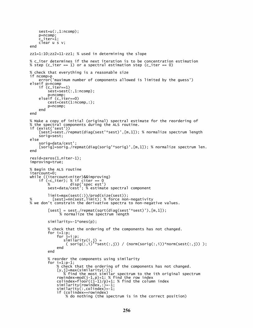
256
sest=u(:,1:ncomp); p=ncomp; c_iter=1; clear u s v; end zz1=1:10;zz2=11-zz1; % used in determining the slope % c_iter determines if the next iteration is to be concentration estimation % step (c_iter == 1) or a spectral estimation step (c_iter == 0) % check that everything is a reasonable size if ncomp>p error('maximum number of components allowed is limited by the guess') elseif p>ncomp if (c_iter==1) sest=sest(:,1:ncomp); p=ncomp; elseif (c_iter==0) cest=cest(1:ncomp,:); p=ncomp; end end % Make a copy of initial (original) spectral estimate for the reordering of % the spectral components during the ALS routine. if (exist('sest')) [sest]=sest./repmat(diag(sest'*sest)',[m,1]); % normalize spectrum length sorig=sest; else sorig=data/cest'; [sorig]=sorig./repmat(diag(sorig'*sorig)',[m,1]); % normalize spectrum len. end resid=zeros(1,niter-1); improving=true; % Begin the ALS routine itercount=0; while ((itercount<niter)&&improving) if (~c_iter); % if citer == 0 % disp('spec est') sest=data/cest'; % estimate spectral component limit=max(sest(:))/prod(size(sest)); % [sest]=nn(sest,limit); % force non-negativity % we don't constrain the derivative spectra to non-negative values. [sest] = sest./repmat(sqrt(diag(sest'*sest)'),[m,1]);
% normalize the spectrum length similarity=-1*ones(p); % check that the ordering of the components has not changed. for i=1:p; for j=i:p; similarity(i,j) = ( sorig(:,i)'*sest(:,j)) / (norm(sorig(:,i))*norm(sest(:,j)) ); end end % reorder the components using similarity for i=1:p-1; % check that the ordering of the components has not changed. [y,j]=max(similarity(:)); % find the most similar spectrum to the ith original spectrum rowindex=mod(j-1,p)+1; % find the row index colindex=floor((j-1)/p)+1; % find the column index similarity(rowindex,:)=-1; similarity(:,colindex)=-1; if (colindex==rowindex) % do nothing (the spectrum is in the correct position)
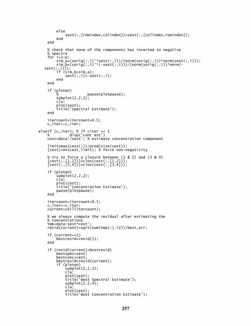
257
else sest(:,[rowindex,colindex])=sest(:,[colindex,rowindex]); end end % check that none of the components has inverted to negative % spectra for i=1:p; sim_a=(sorig(:,i)'*sest(:,i))/(norm(sorig(:,i))*norm(sest(:,i))); sim_b=(sorig(:,i)'*(-sest(:,i)))/(norm(sorig(:,i))*norm(-
sest(:,i))); if (sim_b>sim_a); sest(:,i)=-sest(:,i); end end if (ploten) % pause(plotpause); subplot(2,2,1); cla; plot(sest); title('Spectral Estimate'); end itercount=itercount+0.5; c_iter=~c_iter; elseif (c_iter); % if citer == 1 % disp('conc est') cest=data'/sest'; % estimate concentration component limit=max(cest(:))/prod(size(cest)); [cest]=nn(cest,limit); % force non-negativity % try to force a closure between (1 & 2) and (3 & 4) [cest(:,[1,2])]=clos(cest(:,[1,2])); [cest(:,[3,4])]=clos(cest(:,[3,4])); if (ploten) subplot(2,2,2); cla; plot(cest); title('Concentration Estimate'); pause(plotpause); end itercount=itercount+0.5; c_iter=~c_iter; current=ceil(itercount); % we always compute the residual after estimating the % concentrations tmp=data-sest*cest'; resid(current)=sqrt(sum(tmp(:).^2))/best_err; if (current==1) bestresid=resid(1); end if (resid(current)<bestresid) bestspec=sest; bestconc=cest; bestresid=resid(current); if (ploten) subplot(2,2,3); cla; plot(sest); title('Best Spectral Estimate'); subplot(2,2,4); cla; plot(cest); title('Best Concentration Estimate');
258
end end if (current>12) slope = abs( [resid(current) - ([zz1]*resid(current-(zz2))')/55] );
% weighted average of the last 10 iterations if (slope<0.00001); disp( ['MCR terminated, the slope change was ', num2str(slope)] ) % we have reached a period of little change... end the routine % things are neither getting much worse nor getting much better improving=false; % disp('stopped improving') end end end end conc=cest; spec=sest; % resid=resid/best_err; % return the residual ratioed with respect to the minimal possible error for a
n-component estimate resid=resid(find(resid)); % get rid of any non-allocated residual values if ~exist('bestconc') bestspec=sest; bestconc=cest; bestresid=resid(current); end function [data]=nn(data,limit) % apply an exponential non-negativity constraint to all data points with a % magnitude <= limit. % (this forces all negative values to a constrained positive domain) i=find(data<=limit); data(i)=limit*10.^(data(i)-limit); function [data]=clos(data); % try to find a coefficient so that the % std(coef*data(:,1)+data(:,2)) is minimized. e=zeros(100,1); for i=1:100; e(i)=std((i/2)*data(:,1)+data(:,2)); end [y,t]=min(e); t1=(t-1)/2; % t2=(t+1)/2; for i=1:100; e(i)=std( (t1+ (i/100))*data(:,1)+data(:,2)); end [y,t2]=min(e); t2=t1+((t2)/100); if ((t2>0) & (t2<50)) data(:,1)=t2*data(:,1); end
259
Appendix E: N-Way Visualization Manuscript Reprint
As part of the course of study exploring spectroscopy in turbid
media, methods for visualizing complex multidimensional data were
developed. One such visualization method was published, and a reprint of
the manuscript as published has been included here with permission from
Elsevier. This reprint has been included partly because this is an efficient
way of exploring n-way data sets, and partly because the work was
completed as part of the course of study described in this thesis. The
n-way visualization method is complementary to the work presented,
because prior to the application of any data processing method, the
unprocessed data should be examined to confirm that chemically
significant changes can be observed. Whether 2-D (images, spectra) or
N-D data is recorded, n-way visualization of correlation is a straightforward
way to observe trends in complex datasets. The n-way visualization
method is not used to correct for light-scattering, and so it is included as
an appendix rather than in the main body of the thesis.
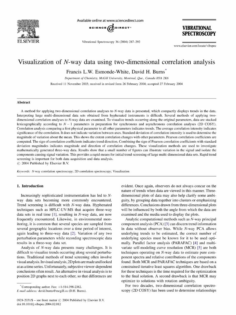
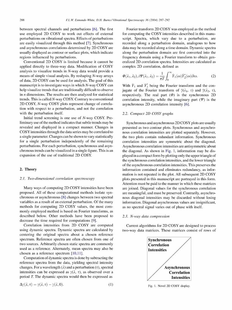
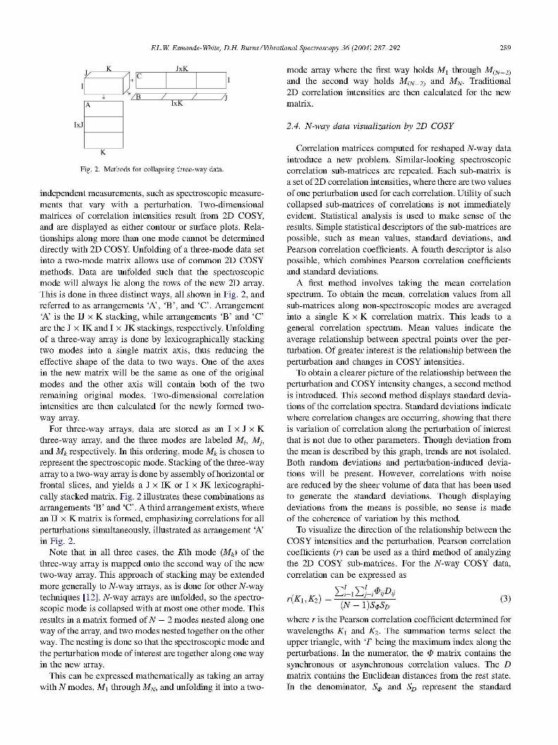
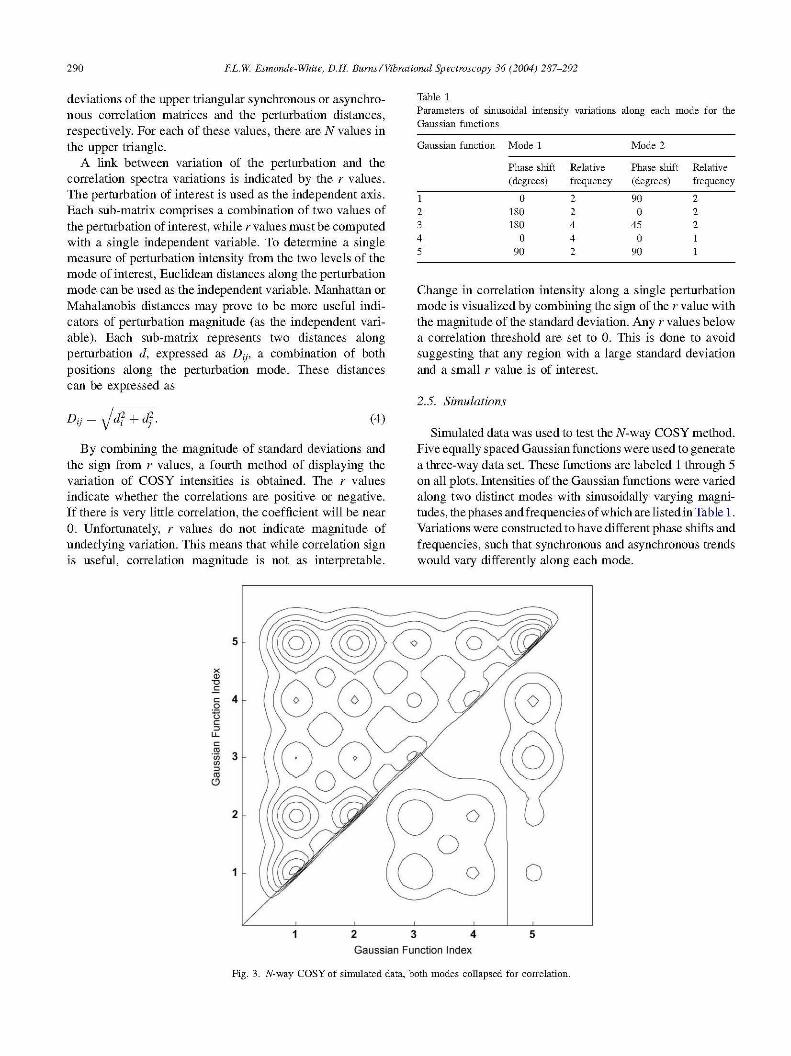
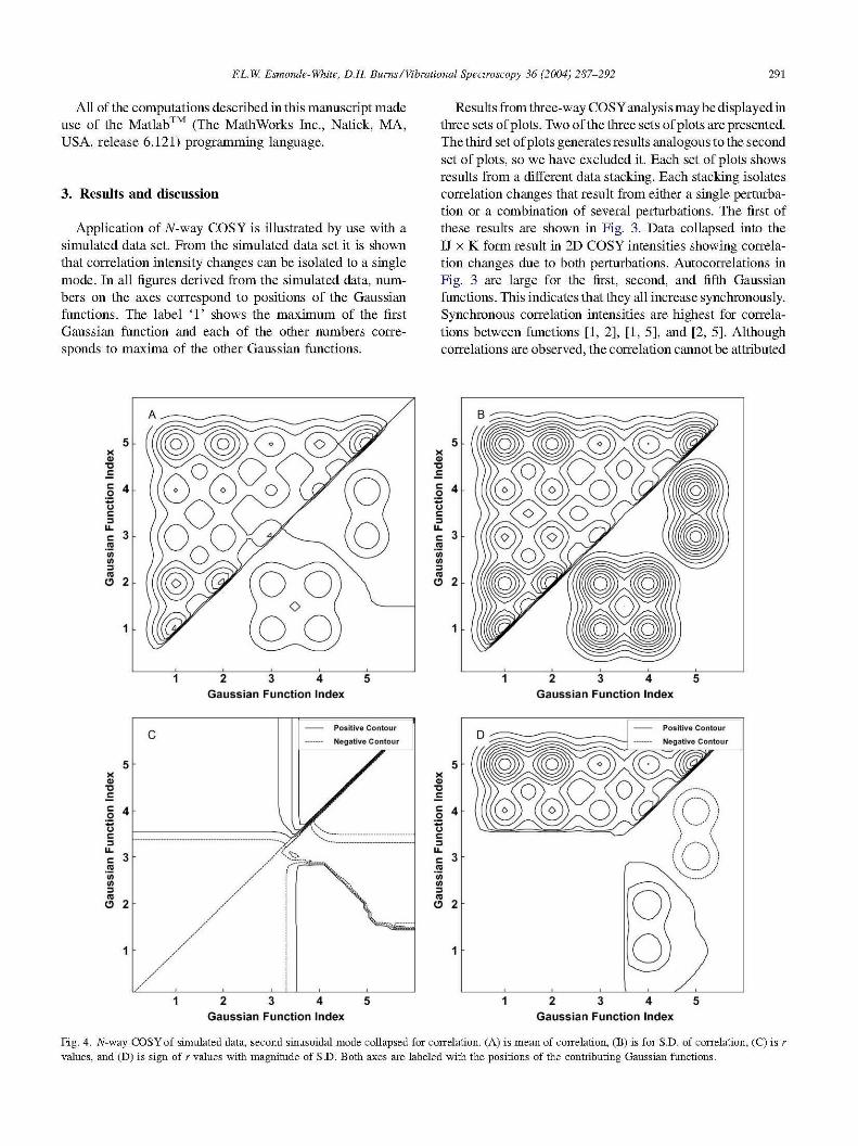
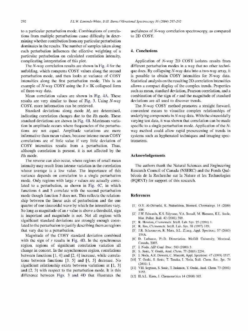
266
Appendix F: Tissue Simulating Phantoms
Because of the difficulties inherent in measuring optical properties
of tissues, calibration materials made from synthetic or natural component
can be used to develop or validate spectroscopic methods used to
analyze scattering media. Optical properties of these calibration materials,
also called tissue phantoms, optical properties can be changed to suit the
requirements of the application. Tissue phantoms can be prepared as
either a liquid or a solid. Properties of tissue phantoms were reviewed by
Pogue and Patterson.251 Several materials are suitable for scattering
calibration method development. Briefly, scattering agents include lipid
emulsions, polymer microspheres, and small particles. Various absorbing
species can be added to the scattering agent, including dyes, inks,
molecular probes, or biological constituents like hemoglobin. One
difference between solid and liquid phantoms is the absence of laser
speckle in the liquid phantoms. Scattering from biological tissue yields
speckle, and some instrumentation uses speckle, while with other
instrumentation speckle may deleteriously influence results.
Lipid emulsions, such as oil-in-water emulsions, milks, and
creams,252 are commonly used as light scattering standards because lipid
bilayers are a primary source of light scattering. Lipid emulsions are
267
popular because the chemical and optical properties of lipid droplets are
similar to lipid bilayers. Moreover, the optical scattering properties of
Intralipid under storage conditions is stable over a long time period
because the polydispersity does not appreciably change.253 However,
once removed from packaging, lipid solutions degrade via oxidation over a
period of hours to days.254 As a result, mixtures containing emulsions must
be prepared immediately before each experiment. Optical properties of
Intralipid are difficult to characterize because particle sizes and
distributions are difficult to measure and widely vary among .255 Due to
pharmaceutical applications and risks of lung embolism from large
droplets, pharmaceutical preparations have well regulated droplet size
distributions. Instruments used for characterizing particle size distributions
of complex mixtures such as oil in water emulsions show variations
between instrument manufacturers and methods.256
Intralipid™ is a commercially available lipid emulsion used for
intravenous feeding. Optical properties of Intralipid have been reported for
a variety of concentrations,113, 167, 169, 257-259 and they demonstrate that
tissue simulating phantoms can be prepared from Intralipid solutions to
accurately describe the optical properties of tissue.
268
The main advantages of using Intralipid as a scattering standard
are the low cost, widespread availability, and the ease of preparing liquid
scattering phantoms into which water-soluble dyes can be incorporated.
The main disadvantages are potential batch-to-batch variations of optical
coefficients, and the limited stability of samples in ambient conditions.
Several other tissue phantoms have been developed, including
solid polyurethane TiO2 phantoms,260 solid glass spheres in polyester
resin,261 aqueous suspensions of polystyrene spheres,262 and Intralipid in
an agar matrix.263 Plastic resin samples can be machined to particular
shapes, and may be particularly suitable for preparing standards that last
for a long time.
269
Appendix G: Numerical Models of Light Scattering
Aside from the purely theoretical approaches used in radiative
transfer theory, diffusion theory, and the 2-flux theories, numerical models
are commonly used to give approximate solutions for scattered light
intensity. The two common methods, finite element analysis and Monte
Carlo simulations are described here.
G.1 Finite Element Analysis
Finite-element analysis is a theoretical approach for modelling light
transport according to a mesh-based diffusion system with nodes through
which photon transport can be calculated.166 Finite-element analysis
systems are used to solve both the forward and inverse problems.166, 264
The forward problem is to calculate how light will propagate through a
system of known properties. The inverse problem is to estimate the
properties of a system using the measured optical response. Results have
shown that this type of analysis can be used to estimate the optical
properties of systems.166 For optimal results, a priori spatial information
(i.e. spatial priors, or estimates of the sample geometry) are incorporated
into the calculations, and require extra information not typically available,
such as geometric mesh-models of the physical system.265, 266 Geometric
models of tissue can be obtained, using optical computed tomography for

270
very shallow tissues, or x-ray computed tomography for deep tissues
Finite element analysis is also computationally expensive.
G.2 Monte Carlo Simulations
Monte Carlo simulations are another approach to estimating the
propagation of light in turbid media using numerical simulation methods.41,
267-270 Photon migration is modeled stochastically in Monte Carlo
simulations by simulating large numbers of photons travelling through the
medium and integrating the results. This is a tractable method for
simulating the motion of light in situations which are too complex to be
solved mathematically. Trajectories for each photon are simulated
according to the transmission and absorption properties of the medium.
Simulations consist of a series of events where individual photons can be:
consumed by absorption, transmitted at a new angle by scattering events,
or escape the simulation boundaries.
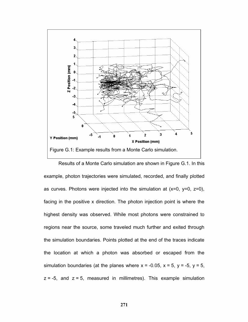
271
Results of a Monte Carlo simulation are shown in Figure G.1. In this
example, photon trajectories were simulated, recorded, and finally plotted
as curves. Photons were injected into the simulation at (x=0, y=0, z=0),
facing in the positive x direction. The photon injection point is where the
highest density was observed. While most photons were constrained to
regions near the source, some traveled much further and exited through
the simulation boundaries. Points plotted at the end of the traces indicate
the location at which a photon was absorbed or escaped from the
simulation boundaries (at the planes where x = -0.05, x = 5, y = -5, y = 5,
z = -5, and z = 5, measured in millimetres). This example simulation
Figure G.1: Example results from a Monte Carlo simulation.
272
shows the results of only 50 photons, while complete simulations might
average the results of 104 or 106 simulated photons.
Accuracy of Monte-Carlo simulations depends greatly on the quality
of the underlying statistical model and the number of photons used in the
simulation. Flux densities, temporal and spatial reflectance profiles, and
sample heating can be also modeled using this type of simulation. Despite
the accuracy of Monte Carlo simulations for estimating how light
propagates, they cannot easily be used to estimate optical properties from
a set of measured experimental results. This “inversion problem” has been
approached by fitting measured distributions to libraries of pre-determined
fluence distributions.271 Libraries consist of a large number of Monte Carlo
models generated with various optical properties for a particular geometry.
273
Bibliography
1. L. Leonardi, and D. H. Burns, "Quantitative Multiwavelength
Constituent Measurements Using Single-Wavelength Photon Time-of-
Flight Correction," Applied Spectroscopy 53, 637-646 (1999).
2. J. D. Ingle, and S. R. Crouch, Spectrochemical analysis (Prentice
Hall, Englewood Cliffs, N.J., 1988).
3. D. A. Skoog, F. J. Holler, and S. R. Crouch, Principles of
instrumental analysis (Thomson Brooks/Cole, Belmont, CA, 2007).
4. A. K. Popp, M. T. Valentine, P. D. Kaplan, and D. A. Weitz,
"Microscopic Origin of Light Scattering in Tissue," Applied Optics 42,
2871-2880 (2003).
5. P. C. Waterman, "Matrix formulation of electromagnetic scattering,"
Proceedings of the IEEE 53, 805-812 (1965).
6. A. Ishimaru, Wave propagation and scattering in random media
(IEEE Press; Oxford University Press, New York; Oxford, 1997).
7. T. Vo-Dinh, ed. Biomedical photonics handbook (CRC Press, Boca
Raton, Fla., 2003).
8. C. F. Bohren, and D. R. Huffman, Absorption and scattering of light
by small particles (Wiley, New York, 1983).
9. M. S. Patterson, B. C. Wilson, and D. R. Wyman, "The propagation
of optical radiation in tissue. II: Optical properties of tissues and resulting
fluence distributions," Lasers in Medical Science 6, 379-390 (1991).
10. S. J. Matcher, M. Cope, and D. T. Delpy, "In vivo measurements of
the wavelength dependence of tissue-scattering coefficients between 760
and 900 nm measured with time-resolved spectroscopy," Applied Optics
36, 386-396 (1997).
11. M. Born, and E. Wolf, Principles of optics: electromagnetic theory of
propagation, interference and diffraction of light (Cambridge University
Press, Cambridge ; New York, 1999).
274
12. W. F. Cheong, S. A. Prahl, and A. J. Welch, "A review of the optical
properties of biological tissues," Quantum Electronics, IEEE Journal of 26,
2166-2185 (1990).
13. A. Liebert, H. Wabnitz, D. Grosenick, M. Möller, R. Macdonald, and
H. Rinneberg, "Evaluation of Optical Properties of Highly Scattering Media
by Moments of Distributions of Times of Flight of Photons," Applied Optics
42, 5785-5792 (2003).
14. G. W. Faris, "Diffusion equation boundary conditions for the
interface between turbid media: a comment," J. Opt. Soc. Am. A 19, 519-
520 (2002).
15. G. N. K. Y. Tatsuya Nakai, "Expression of optical diffusion
coefficient in high-absorption turbid media," Electronics and
Communications in Japan (Part II: Electronics) 81, 34-41 (1998).
16. I. V. Yaroslavsky, A. N. Yaroslavsky, V. V. Tuchin, and H.-J.
Schwarzmaier, "Effect of the scattering delay on time-dependent photon
migration in turbid media," Applied Optics 36, 6529-6538 (1997).
17. C. A. Thompson, K. J. Webb, and A. M. Weiner, "Diffusive media
characterization with laser speckle," Applied Optics 36, 3726-3734 (1997).
18. A. Kienle, and M. S. Patterson, "Improved solutions of the steady-
state and the time-resolved diffusion equations for reflectance from a
semi-infinite turbid medium," J. Opt. Soc. Am. A 14, 246-254 (1997).
19. R. Model, R. Huenlich, D. Richter, H. H. Rinneberg, H. Wabnitz,
and M. Walzel, "Imaging in random media: simulating light transport by
numerical integration of the diffusion equation," in Photon Transport in
Highly Scattering Tissue, (SPIE, Lille, France, 1995), pp. 11-22.
20. R. C. Haskell, L. O. Svaasand, T.-T. Tsay, T.-C. Feng, M. S.
McAdams, and B. J. Tromberg, "Boundary conditions for the diffusion
equation in radiative transfer," J. Opt. Soc. Am. A 11, 2727- (1994).
21. G. Yoon, A. Welch, M. Motamedi, and M. v. Gemert, "Development
and application of three-dimensional light distribution model for laser
275
irradiated tissue," Quantum Electronics, IEEE Journal of 23, 1721-1733
(1987).
22. M. Keijzer, W. M. Star, and P. R. M. Storchi, "Optical diffusion in
layered media," Applied Optics 27, 1820 (1988).
23. M. S. C. Patterson, B.; Wilson, Brian C., "Time resolved reflectance
and transmittance for the noninvasive measurement of tissue optical
properties," Applied Optics 28, 2331-2336 (1989).
24. V. V. Tuchin, "Light scattering study of tissues," Physics-Uspekhi
40, 495-515 (1997).
25. S. J. Madsen, B. C. Wilson, M. S. Patterson, Y. D. Park, S. L.
Jacques, and Y. Hefetz, "Experimental tests of a simple diffusion model
for the estimation of scattering and absorption coefficients of turbid media
from time resolved diffuse reflectance measurements," Applied Optics 31,
3509-3517 (1992).
26. T. J. Farrell, M. S. Patterson, and B. Wilson, "A diffusion theory
model of spatially resolved, steady-state diffuse reflectance for the
noninvasive determination of tissue optical properties in vivo," Medical
Physics 19, 879-888 (1992).
27. D. T. Delpy, and M. Cope, "Quantification in tissue near-infrared
spectroscopy," Philosophical Transactions of the Royal Society B:
Biological Sciences 352, 649-659 (1997).
28. R. Richards-Kortum, and E. Sevick-Muraca, "Quantitative optical
spectroscopy for tissue diagnosis," Annual Review of Physical Chemistry
47, 555-606 (1996).
29. R. A. J. Groenhuis, J. J. Ten Bosch, and H. A. Ferwerda,
"Scattering and absorption of turbid materials determined from reflection
measurements. 2: Measuring method and calibration," Applied Optics 22,
2463 (1983).
30. M. G. Nichols, E. L. Hull, and T. H. Foster, "Design and testing of a
white-light, steady-state diffuse reflectance spectrometer for determination

276
of optical properties of highly scattering systems," Applied Optics 36, 93-
104 (1997).
31. R. M. P. Doornbos, R. Lang, M. C. Aalders, F. W. Cross, and H. J.
C. M. Sterenborg, "The determination of in vivo human tissue optical
properties and absolute chromophore concentrations using spatially
resolved steady-state diffuse reflectance spectroscopy," Physics in
Medicine and Biology, 967 (1999).
32. S. Nickell, M. Hermann, M. Essenpreis, T. J. Farrell, U. Kramer,
and M. S. Patterson, "Anisotropy of light propagation in human skin,"
Physics in Medicine and Biology, 2873 (2000).
33. J. Swartling, J. S. Dam, and S. Andersson-Engels, "Comparison of
Spatially and Temporally Resolved Diffuse-Reflectance Measurement
Systems for Determination of Biomedical Optical Properties," Applied
Optics 42, 4612-4620 (2003).
34. L. Wang, and S. L. Jacques, "Use of a laser beam with an oblique
angle of incidence to measure the reduced scattering coefficient of a
turbid medium," Applied Optics 34, 2362-2366 (1995).
35. A. Kienle, L. Lilge, M. S. Patterson, R. Hibst, R. Steiner, and B. C.
Wilson, "Spatially resolved absolute diffuse reflectance measurements for
noninvasive determination of the optical scattering and absorption
coefficients of biological tissue," Applied Optics 35, 2304-2314 (1996).
36. L. Gobin, L. Blanchot, and H. Saint-Jalmes, "Integrating the
Digitized Backscattered Image to Measure Absorption and Reduced-
Scattering Coefficients in vivo," Applied Optics 38, 4217-4227 (1999).
37. T. H. Pham, F. Bevilacqua, T. Spott, J. S. Dam, B. J. Tromberg,
and S. Andersson-Engels, "Quantifying the absorption and reduced
scattering coefficients of tissuelike turbid media over a broad spectral
range with noncontact Fourier-transform hyperspectral imaging," Applied
Optics 39, 6487-6497 (2000).
277
38. N. Joshi, C. Donner, and H. W. Jensen, "Noninvasive measurement
of scattering anisotropy in turbid materials by nonnormal incident
illumination," Optics Letters 31, 936-938 (2006).
39. R. A. J. Groenhuis, H. A. Ferwerda, and J. J. Ten Bosch,
"Scattering and absorption of turbid materials determined from reflection
measurements. 1: Theory," Applied Optics 22, 2456 (1983).
40. M. E. Arnoldussen, D. Cohen, G. H. Bearman, and W. S.
Grundfest, "Consequences of scattering for spectral imaging of turbid
biologic tissue," Journal of Biomedical Optics 5, 300-306 (2000).
41. D. T. Delpy, M. Cope, P. v. d. Zee, S. Arridge, S. Wray, and J.
Wyatt, "Estimation of optical pathlength through tissue from direct time of
flight measurement," Physics in Medicine and Biology 33, 1433-1442
(1988).
42. M. S. Patterson, J. D. Moulton, B. C. Wilson, and B. Chance,
"Applications of time-resolved light scattering measurements to
photodynamic therapy dosimetry," in Photodynamic Therapy: Mechanisms
II, (SPIE, Los Angeles, CA, USA, 1990), pp. 62-75.
43. F. Liu, K. M. Yoo, and R. R. Alfano, "Ultrafast laser-pulse
transmission and imaging through biological tissues," Appl. Opt. 32, 554-
558 (1993).
44. D. Mathur, "Matter in strong fields: from molecules to living cells,"
Journal of Physics: Conference Series, 012048 (2007).
45. B. J. Tromberg, N. Shah, R. Lanning, A. Cerussi, J. Espinoza, T.
Pham, L. Svaasand, and J. Butler, "Non-invasive in vivo characterization
of breast tumors using photon migration spectroscopy," Neoplasia 2, 26-
40 (2000).
46. B. W. Pogue, and M. S. Patterson, "Frequency-domain optical
absorption spectroscopy of finite tissue volumes using diffusion theory,"
Physics in medicine & biology 39, 1157-1180 (1994).
278
47. B. W. Pogue, S. Jiang, H. Dehghani, C. Kogel, S. Soho, S.
Srinivasan, X. Song, T. D. Tosteson, S. P. Poplack, and K. D. Paulsen,
"Characterization of hemoglobin, water, and NIR scattering in breast
tissue: analysis of intersubject variability and menstrual cycle changes,"
Journal of Biomedical Optics 9, 541-552 (2004).
48. F. Blais, "Review of 20 years of range sensor development,"
Journal of electronic imaging 13, 231 (2004).
49. S. Yamaguchi, "Convenient Method of Measuring the Chirp
Structure of Femtosecond White-Light Continuum Pulses," Applied
Spectroscopy 49, 1513 (1995).
50. A. M. Zheltikov, "Let there be white light: supercontinuum
generation by ultrashort laser pulses," Physics-Uspekhi, 605 (2006).
51. G. r. Genty, "Supercontinuum generation in microstructured fibers
and novel optical measurement techniques," (Helsinki University of
Technology, Espoo, 2004).
52. R. L. Fork, C. V. Shank, C. Hirlimann, R. Yen, and W. J. Tomlinson,
"Femtosecond white-light continuum pulses," Opt. Lett. 8, 1-3 (1983).
53. S. Andersson-Engels, R. Berg, A. Persson, and S. Svanberg,
"Multispectral tissue characterization with time-resolved detection of
diffusely scattered white light," Opt. Lett. 18, 1697-1699 (1993).
54. S. A. Trushin, W. Fuss, K. Kosma, and W. E. Schmid, "Widely
tunable ultraviolet sub-30-fs pulses from supercontinuum for transient
spectroscopy," Applied Physics B: Lasers and Optics 85, 1-5 (2006).
55. R. R. Alfano, "Emission in the Region 4000 to 7000 Å Via Four-
Photon Coupling in Glass," Physical Review Letters 24, 584 (1970).
56. J. K. Ranka, R. S. Windeler, and A. J. Stentz, "Visible continuum
generation in air-silica microstructure optical fibers with anomalous
dispersion at 800 nm," Optics letters 25, 25-27 (2000).
57. K. Lindfors, T. Kalkbrenner, P. Stoller, and V. Sandoghdar,
"Detection and Spectroscopy of Gold Nanoparticles Using
279
Supercontinuum White Light Confocal Microscopy," Physical Review
Letters 93, 037401 (2004).
58. T. A. Birks, W. J. Wadsworth, and P. S. Russell, "Supercontinuum
generation in tapered fibers," Optics letters 25, 1415-1417 (2000).
59. T. H. Pham, O. Coquoz, J. B. Fishkin, E. Anderson, and B. J.
Tromberg, "Broad bandwidth frequency domain instrument for quantitative
tissue optical spectroscopy," Review of Scientific Instruments 71, 2500-
2513 (2000).
60. B. Chance, "Time-resolved spectroscopy and imaging," in Optical
Tomography, Photon Migration, and Spectroscopy of Tissue and Model
Media: Theory, Human Studies, and Instrumentation, (SPIE, San Jose,
CA, USA, 1995), pp. 122-139.
61. S. J. Madsen, E. R. Anderson, R. C. Haskell, and B. J. Tromberg,
"Portable, high-bandwidth frequency-domain photon migration instrument
for tissue spectroscopy," Opt. Lett. 19, 1934-1936 (1994).
62. S. R. Arridge, M. Cope, and D. T. Delpy, "The theoretical basis for
the determination of optical pathlengths in tissue: temporal and frequency
analysis," Physics in Medicine and Biology, 1531 (1992).
63. E. M. Sevick, B. Chance, J. Leigh, S. Nioka, and M. Maris,
"Quantitation of time- and frequency-resolved optical spectra for the
determination of tissue oxygenation," Analytical Biochemistry 195, 330-
351 (1991).
64. S. Fantini, "Frequency-domain multichannel optical detector for
noninvasive tissue spectroscopy and oximetry," Optical engineering 34, 32
(1995).
65. D. H. Burns, "Optical Tomography for Three-Dimensional
Spectroscopy," Applied Spectroscopy 48, 12 (1994).
66. W. F. Long, C. E. W. Gributs, and D. H. Burns, "Quantification in
highly scattering/absorbing layered samples using photon time-of-flight
280
measurements and confocal optical geometry," Vibrational Spectroscopy
30, 121-129 (2002).
67. G. Boverman, Q. Fang, S. A. Carp, E. L. Miller, D. H. Brooks, J.
Selb, R. H. Moore, D. B. Kopans, and D. A. Boas, "Spatio-temporal
imaging of the hemoglobin in the compressed breast with diffuse optical
tomography," Physics in Medicine and Biology, 3619 (2007).
68. S. Srinivasan, B. W. Pogue, S. Jiang, H. Dehghani, C. Kogel, S.
Soho, J. J. Gibson, T. D. Tosteson, S. P. Poplack, and K. D. Paulsen,
"Interpreting hemoglobin and water concentration, oxygen saturation, and
scattering measured in vivo by near-infrared breast tomography,"
Proceedings of the National Academy of Sciences 100, 12349-12354
(2003).
69. T. O. McBride, B. W. Pogue, S. Poplack, S. Soho, W. A. Wells, S.
Jiang, U. L. Osterberg, and K. D. Paulsen, "Multispectral near-infrared
tomography: a case study in compensating for water and lipid content in
hemoglobin imaging of the breast," Journal of Biomedical Optics 7, 72-79
(2002).
70. D. A. Benaron, M. Lennox, and D. K. Stevenson, "Two-dimensional
and 3-D images of thick tissue using time-constrained times-of-flight and
absorbance spectrophotometry," in Physiological Monitoring and Early
Detection Diagnostic Methods, (SPIE, Los Angeles, CA, USA, 1992), pp.
35-45.
71. D. Huang, E. A. Swanson, C. P. Lin, J. S. Schuman, W. G. Stinson,
W. Chang, M. R. Hee, T. Flotte, K. Gregory, and C. A. Puliafito, "Optical
coherence tomography," Science 254, 1178-1181 (1991).
72. A. M. Rollins, and J. A. Izatt, "Optimal interferometer designs for
optical coherence tomography," Optics letters 24, 1484-1486 (1999).
73. J. M. Schmitt, "Optical coherence tomography (OCT): a review,"
IEEE journal of selected topics in quantum electronics 5, 1205 (1999).
281
74. W. Watanabe, Y. Masuda, and K. Itoh, "Coherence
Spectrotomography of Layered Medium with White-Light Continuum,"
Optical Review 6, 71-76 (1999).
75. A. F. Fercher, "Optical coherence tomography-principles and
applications," Reports on Progress in Physics 66, 239 (2003).
76. W. Drexler, "Ultrahigh-resolution optical coherence tomography,"
Journal of biomedical optics 9, 47 (2004).
77. D. A. Boas, D. H. Brooks, E. L. Miller, C. A. DiMarzio, M. Kilmer, R.
J. Gaudette, and Z. Quan, "Imaging the body with diffuse optical
tomography," Signal Processing Magazine, IEEE 18, 57-75 (2001).
78. J.-L. Boulnois, "Photophysical processes in recent medical laser
developments: A review," Lasers in Medical Science 1, 47-66 (1986).
79. B. C. Wilson, "Time-dependent optical spectroscopy and imaging
for biomedical applications," Proceedings of the IEEE 80, 918 (1992).
80. B. C. Wilson, "Optical reflectance and transmittance of tissues:
principles and applications," IEEE journal of quantum electronics 26, 2186
(1990).
81. S. Andersson-Engels, J. Axelsson, A. Johansson, J. Johansson, S.
Svanberg, and T. Svensson, "Time-of-flight laser spectroscopy in
biomedical diagnostics," in Optical Fiber Communication and
Optoelectronics Conference, 2007 Asia, (2007), pp. 236-238.
82. R. R. Alfano, "Advances in Optical Imaging of Biomedical Media,"
Annals of the New York Academy of Sciences 820, 248 (1997).
83. S. J. Matcher, "Performance Comparison of Several Published
Tissue Near-Infrared Spectroscopy Algorithms," Analytical Biochemistry
227, 54 (1995).
84. R. X. Xu, B. Qiang, J. J. Mao, and S. P. Povoski, "Development of a
handheld near-infrared imager for dynamic characterization of in vivo
biological tissue systems," Applied Optics 46, 7442-7451 (2007).
282
85. T. Shiga, K. Yamamoto, K. Tanabe, Y. Nakase, and B. Chance,
"Study of an algorithm based on model experiments and diffusion theory
for a portable tissue oximeter," Journal of Biomedical Optics 2, 154-161
(1997).
86. B. Grassi, V. Quaresima, C. Marconi, M. Ferrari, and P. Cerretelli,
"Blood lactate accumulation and muscle deoxygenation during incremental
exercise," J Appl Physiol 87, 348-355 (1999).
87. N. J. Crane, Z. D. Schultz, and I. W. Levin, "Contrast Enhancement
for in Vivo Visible Reflectance Imaging of Tissue Oxygenation," Appl.
Spectrosc. 61, 797-803 (2007).
88. S. P. Nighswander-Rempel, V. V. Kupriyanov, and R. A. Shaw,
"Regional cardiac tissue oxygenation as a function of blood flow and pO2:
a near-infrared spectroscopic imaging study," Journal of Biomedical Optics
11, 054004-054010 (2006).
89. P. Rolfe, "In vivo near-infrared spectroscopy," Annual Review of
Biomedical Engineering 2, 715-754 (2000).
90. J. Gade, D. Palmqvist, P. Plomgard, and G. Greisen, "Diffuse
reflectance spectrophotometry with visible light: comparison of four
different methods in a tissue phantom," Physics in Medicine and Biology
51, 121-136 (2006).
91. R. J. McNichols, and G. L. Cote, "Optical glucose sensing in
biological fluids: an overview," Journal of Biomedical Optics 5, 5-16
(2000).
92. A. D. McGown, H. Makker, C. Elwell, P. G. Al Rawi, A. Valipour,
and S. G. Spiro, "Measurement of Changes in Cytochrome Oxidase
Redox State During Obstructive Sleep Apnea Using Near-Infrared
Spectroscopy," Sleep 26, 1-7 (2003).
93. L. S. L. Arakaki, "An Optical Method for Myoglobin Oxygenenation
Measurements in the Blood-Perfused Rat Hind Limb," in Center for
Bioengineering, (University of Washington, Seattle, 1995), p. 161.
283
94. H. Xu, B. W. Pogue, H. Dehghani, K. D. Paulsen, R. Springett, and
J. F. Dunn, "Absorption and scattering imaging of tissue with steady-state
second-differential spectral-analysis tomography," Optics Letters 29,
2043-2045 (2004).
95. D. Lafrance, L. C. Lands, and D. H. Burns, "In vivo lactate
measurement in human tissue by near-infrared diffuse reflectance
spectroscopy," Vibrational Spectroscopy 36, 195-202 (2004).
96. D. J. Marcinek, W. A. Ciesielski, K. E. Conley, and K. A.
Schenkman, "Oxygen regulation and limitation to cellular respiration in
mouse skeletal muscle in vivo," Am J Physiol Heart Circ Physiol 285,
H1900-1908 (2003).
97. K. A. Schenkman, Marble, D.R., Burns, D.H., Feigl, E.O., "Optical
Spectroscopic Method for in Vivo Measurement of Cardiac Myoglobin
Oxygen Saturation," Applied Spectroscopy 53, 332-338 (1999).
98. M. G. Sowa, L. Leonardi, J. R. Payette, K. M. Cross, M. Gomez,
and J. S. Fish, "Classification of burn injuries using near-infrared
spectroscopy," Journal of Biomedical Optics 11, 054002-054006 (2006).
99. J. Wang, Y.-J. Geng, B. Guo, T. Klima, B. N. Lal, J. T. Willerson,
and W. Casscells, "Near-infrared spectroscopic characterization of human
advanced atherosclerotic plaques," J Am Coll Cardiol 39, 1305-1313
(2002).
100. M. M. Tisdall, I. Tachtsidis, T. S. Leung, C. E. Elwell, and M. Smith,
"Near-infrared spectroscopic quantification of changes in the concentration
of oxidized cytochrome c oxidase in the healthy human brain during
hypoxemia," Journal of Biomedical Optics 12, 024002-024007 (2007).
101. J. Hoffmann, D. W. Lubbers, and H. M. Heise, "Applicability of the
Kubelka-Munk theory for the evaluation of reflectance spectra
demonstrated for haemoglobin-free perfused heart tissue," Physics in
Medicine and Biology 43, 3571-3587 (1998).
284
102. D. J. Dahm, and K. D. Dahm, "Representative Layer Theory for
Diffuse Reflectance," Applied Spectroscopy 53, 647-654 (1999).
103. B. O. Budevska, S. T. Sum, and T. J. Jones, "Application of
Multivariate Curve Resolution for Analysis of FT-IR Microspectroscopic
Images of in Situ Plant Tissue," Applied Spectroscopy 57, 124-131 (2003).
104. C. E. W. Gributs, and D. H. Burns, "Parsimonious calibration
models for near-infrared spectroscopy using wavelets and scaling
functions," Chemometrics and Intelligent Laboratory Systems 83, 44-53
(2006).
105. B. M. Smith, and P. J. Gemperline, "Wavelength Selection and
Optimization of Pattern Recognition Methods Using the Genetic
Algorithm," Analytica Chimica Acta 423, 167-177 (2000).
106. C. Beleites, G. Steiner, M. G. Sowa, R. Baumgartner, S. Sobottka,
G. Schackert, and R. Salzer, "Classification of human gliomas by infrared
imaging spectroscopy and chemometric image processing," Vibrational
Spectroscopy 38, 143-149 (2005).
107. F. P. Bevilacqua, D. Piguet, P. Marquet, J. D. Gross, B. J.
Tromberg, and C. D. Depeursinge, "In-vivo local determination of tissue
optical properties," in Photon Propagation in Tissues III, (SPIE, San
Remo, Italy, 1998), pp. 262-268.
108. T. Hamaoka, T. Katsumura, N. Murase, S. Nishio, T. Osada, T.
Sako, H. Higuchi, Y. Kurosawa, T. Shimomitsu, M. Miwa, and B. Chance,
"Quantification of ischemic muscle deoxygenation by near infrared time-
resolved spectroscopy," Journal of Biomedical Optics 5, 102-105 (2000).
109. R. Hornung, T. H. Pham, K. A. Keefe, M. W. Berns, Y. Tadir, and B.
J. Tromberg, "Quantitative near-infrared spectroscopy of cervical
dysplasia in vivo," Hum. Reprod. 14, 2908-2916 (1999).
110. A. Cerussi, N. Shah, D. Hsiang, A. Durkin, J. Butler, and B. J.
Tromberg, "In vivo absorption, scattering, and physiologic properties of 58
285
malignant breast tumors determined by broadband diffuse optical
spectroscopy," Journal of Biomedical Optics 11, 044005-044016 (2006).
111. T. J. Beck, W. Beyer, T. Pongratz, W. Stummer, R. M. Waidelich,
H. Stepp, S. Wagner, and R. Baumgartner, "Clinical determination of
tissue optical properties in vivo by spatially resolved reflectance
measurements," in Photon Migration and Diffuse-Light Imaging, (SPIE,
Munich, Germany, 2003), pp. 96-105.
112. F. Chauchard, S. Roussel, J. M. Roger, V. Bellon-Maurel, C.
Abrahamsson, T. Svensson, S. Andersson-Engels, and S. Svanberg,
"Least-squares support vector machines modelization for time-resolved
spectroscopy," Applied Optics 44, 7091-7097 (2005).
113. T. Xu, C. Zhang, X. Wang, L. Zhang, and J. Tian, "Measurement
and Analysis of Light Distribution in Intralipid-10% at 650 nm," Applied
Optics 42, 5777-5784 (2003).
114. H. Owen-Reece, M. Smith, C. E. Elwell, and J. C. Goldstone, "Near
infrared spectroscopy," Br. J. Anaesth. 82, 418-426 (1999).
115. G. Greisen, "Is near-infrared spectroscopy living up to its
promises?," Seminars in Fetal and Neonatal Medicine 11, 498-502 (2006).
116. G. Zaccanti, A. Taddeucci, M. Barilli, P. Bruscaglioni, and F.
Martelli, "Optical properties of biological tissues," in Optical Tomography,
Photon Migration, and Spectroscopy of Tissue and Model Media: Theory,
Human Studies, and Instrumentation, (SPIE, San Jose, CA, USA, 1995),
pp. 513-521.
117. M. J. C. Van Gemert, S. L. Jacques, H. J. C. M. Sterenborg, and W.
M. Star, "Skin optics," Biomedical Engineering, IEEE Transactions on 36,
1146-1154 (1989).
118. L. Stryer, Biochemistry (W.H. Freeman, New York :, 1995).
119. J. B. Wittenberg, "Myoglobin-facilitated oxygen diffusion: role of
myoglobin in oxygen entry into muscle," Physiol. Rev. 50, 559-636 (1970).
286
120. L. S. L. Arakaki, and D. H. Burns, "Multispectral Analysis for
Quantitative Measurements of Myoglobin Oxygen Fractional Saturation in
the Presence of Hemoglobin Interference," Applied Spectroscopy 46,
1919-1928 (1992).
121. S. J. Matcher, P. J. Kirkpatrick, K. Nahid, M. Cope, and D. T. Delpy,
"Absolute quantification methods in tissue near-infrared spectroscopy," in
Optical Tomography, Photon Migration, and Spectroscopy of Tissue and
Model Media: Theory, Human Studies, and Instrumentation, (SPIE, San
Jose, CA, USA, 1995), pp. 486-495.
122. K. A. Schenkman, D. R. Marble, D. H. Burns, and E. O. Feigl,
"Myoglobin oxygen dissociation by multiwavelength spectroscopy," J Appl
Physiol 82, 86-92 (1997).
123. J. C. Maxwell, C. H. Barlow, J. E. Spallholz, and W. S. Caughey,
"The utility of infrared spectroscopy as a probe of intact tissue:
determination of carbon monoxide and hemeproteins in blood and heart
muscle," Biochem Biophys Res Commun 61, 230-236 (1974).
124. F. Costes, J. C. Barthelemy, L. Feasson, T. Busso, A. Geyssant,
and C. Denis, "Comparison of muscle near-infrared spectroscopy and
femoral blood gases during steady-state exercise in humans," J Appl
Physiol 80, 1345-1350 (1996).
125. R. A. Blasi, M. Cope, C. Elwell, F. Safoue, and M. Ferrari,
"Noninvasive measurement of human forearm oxygen consumption by
near infrared spectroscopy," European Journal of Applied Physiology 67,
20-25 (1993).
126. R. Boushel, H. Langberg, J. Olesen, J. Gonzales-Alonzo, J. Bulow,
and M. Kjaer, "Monitoring tissue oxygen availability with near infrared
spectroscopy (NIRS) in health and disease," Scandinavian Journal of
Medicine & Science in Sports 11, 213-222 (2001).
127. M. J. Hayes, and P. R. Smith, "Artifact Reduction in
Photoplethysmography," Applied Optics 37, 7437-7446 (1998).
287
128. G. A. Millikan, "The Oximeter, an Instrument for Measuring
Continuously the Oxygen Saturation of Arterial Blood in Man," Review of
Scientific Instruments 13, 434-444 (1942).
129. G. Zonios, U. Shankar, and V. K. Iyer, "Pulse oximetry theory and
calibration for low saturations," Biomedical Engineering, IEEE
Transactions on 51, 818-822 (2004).
130. J. E. Sinex, "Pulse oximetry: Principles and limitations," The
American Journal of Emergency Medicine 17, 59-66 (1999).
131. J. G. Webster, ed. Design of Pulse Oximeters (Institute of Physics
Publishing, Bristol and Philadelphia, 1997).
132. A. C. Ralston, R. K. Webb, and W. B. Runciman, "Potential errors
in pulse oximetry. I. Pulse oximeter evaluation," Anaesthesia 46, 202-206
(1991).
133. K. Humphreys, T. Ward, and C. Markham, "Noncontact
simultaneous dual wavelength photoplethysmography: A further step
toward noncontact pulse oximetry," Review of Scientific Instruments 78,
044304 (2007).
134. D. M. Mancini, J. R. Wilson, L. Bolinger, H. Li, K. Kendrick, B.
Chance, and J. S. Leigh, "In vivo magnetic resonance spectroscopy
measurement of deoxymyoglobin during exercise in patients with heart
failure. Demonstration of abnormal muscle metabolism despite adequate
oxygenation," Circulation 90, 500-508 (1994).
135. K. A. Schenkman, and W. A. Ciesielski, "Improved Myoglobin
Saturation Measurement Made by Partial Least-Squares Analysis of
Optical Reflectance Spectra," Applied Spectroscopy 56, 1215-1221
(2002).
136. D. J. Marcinek, K. A. Schenkman, W. A. Ciesielski, and K. E.
Conley, "Mitochondrial coupling in vivo in mouse skeletal muscle," Am J
Physiol Cell Physiol 286, C457-463 (2004).
288
137. D. Lafrance, L. C. Lands, L. Hornby, and D. H. Burns, "Near-
Infrared Spectroscopic Measurement of Lactate in Human Plasma,"
Applied Spectroscopy 54, 300-304 (2000).
138. D. Lafrance, L. C. Lands, and D. H. Burns, "Measurement of lactate
in whole human blood with near-infrared transmission spectroscopy,"
Talanta 60, 635-641 (2003).
139. N. Kollias, "The physical basis of skin color and its evaluation,"
Clinics in Dermatology 13, 361-367 (1995).
140. G. N. Stamatas, B. Z. Zmudzka, N. Kollias, and J. Z. Beer, "Non-
Invasive Measurements of Skin Pigmentation In Situ," Pigment Cell
Research 17, 618-626 (2004).
141. I. Nishidate, Y. Aizu, and H. Mishina, "Estimation of melanin and
hemoglobin in skin tissue using multiple regression analysis aided by
Monte Carlo simulation," Journal of Biomedical Optics 9, 700-710 (2004).
142. A. N. Bashkatov, E. A. Genina, V. I. Kochubey, and V. V. Tuchin,
"Optical properties of human skin, subcutaneous and mucous tissues in
the wavelength range from 400 to 2000 nm," Journal of Physics D: Applied
Physics, 2543 (2005).
143. W. Shen, Z. Wang, M. Punyanita, J. Lei, A. Sinav, J. G. Kral, C.
Imielinska, R. Ross, and S. B. Heymsfield, "Adipose Tissue Quantification
by Imaging Methods: A Proposed Classification," Obesity Res 11, 5-16
(2003).
144. J. J. Kelly, K. A. Kelly, and C. H. Barlow, "Tissue temperature by
near-infrared spectroscopy," in Optical Tomography, Photon Migration,
and Spectroscopy of Tissue and Model Media: Theory, Human Studies,
and Instrumentation, (SPIE, San Jose, CA, USA, 1995), pp. 818-828.
145. O. S. Khalil, "Spectroscopic and Clinical Aspects of Noninvasive
Glucose Measurements," Clin Chem 45, 165-177 (1999).
289
146. O. S. Khalil, "Non-invasive glucose measurement technologies: an
update from 1999 to the dawn of the new millennium," Diabetes Technol
Ther 6, 660-697 (2004).
147. J. C. Pickup, F. Hussain, N. D. Evans, and N. Sachedina, "In vivo
glucose monitoring: the clinical reality and the promise," Biosensors and
Bioelectronics 20, 1897-1902 (2005).
148. M. A. Arnold, and G. W. Small, "Noninvasive Glucose Sensing,"
Anal. Chem. 77, 5429-5439 (2005).
149. M. A. Arnold, "Non-invasive glucose monitoring," Current Opinion in
Biotechnology 7, 46-49 (1996).
150. M. R. Robinson, R. P. Eaton, D. M. Haaland, G. W. Koepp, E. V.
Thomas, B. R. Stallard, and P. L. Robinson, "Noninvasive glucose
monitoring in diabetic patients: a preliminary evaluation," Clin Chem 38,
1618-1622 (1992).
151. J. Chen, M. A. Arnold, and G. W. Small, "Comparison of
Combination and First Overtone Spectral Regions for Near-Infrared
Calibration Models for Glucose and Other Biomolecules in Aqueous
Solutions," Anal. Chem. 76, 5405-5413 (2004).
152. K. H. Hazen, M. A. Arnold, and G. W. Small, "Measurement of
glucose and other analytes in undiluted human serum with near-infrared
transmission spectroscopy," Analytica Chimica Acta 371, 255-267 (1998).
153. L. S. L. Arakaki, M. J. Kushmerick, and D. H. Burns, "Myoglobin
Oxygen Saturation Measured Independently of Hemoglobin in Scattering
Media by Optical Reflectance Spectroscopy," Applied Spectroscopy 50,
697-707 (1996).
154. M. Egawa, T. Fukuhara, M. Takahashi, and Y. Ozaki, "Determining
Water Content in Human Nails with a Portable Near-Infrared
Spectrometer," Applied Spectroscopy 57, 473-478 (2003).
155. M. Cope, P. van der Zee, M. Essenpreis, S. R. Arridge, and D. T.
Delpy, "Data analysis methods for near-infrared spectroscopy of tissue:
290
problems in determining the relative cytochrome aa3 concentration," in
Time-Resolved Spectroscopy and Imaging of Tissues, (SPIE, Los
Angeles, CA, USA, 1991), pp. 251-262.
156. B. G. Osborne, "Near-infrared spectroscopy in food analysis," in
Encyclopedia of Analytical Chemistry, R. A. Meyers, ed. (John Wiley &
Sons Ltd., Chichester, 1986), pp. 1-14.
157. M. Blanco, J. Coello, A. Eustaquio, H. Iturriaga, and S. Maspoch,
"Development and validation of a method for the analysis of a
pharmaceutical preparation by near-infrared diffuse reflectance
spectroscopy," Journal of Pharmaceutical Sciences 88, 551-556 (1999).
158. B. D. S. Venz, "NIR-spectroscopic investigation of water sorption
characteristics of dental resins and composites," Journal of Biomedical
Materials Research 25, 1231-1248 (1991).
159. A. E. Cerussi, D. Jakubowski, N. Shah, F. Bevilacqua, R. Lanning,
A. J. Berger, D. Hsiang, J. Butler, R. F. Holcombe, and B. J. Tromberg,
"Spectroscopy enhances the information content of optical
mammography," Journal of Biomedical Optics 7, 60-71 (2002).
160. J. Nyström, B. Lindholm-Sethson, L. Stenberg, S. Ollmar, J.
Eriksson, and P. Geladi, "Combined near-infrared spectroscopy and
multifrequency bio-impedance investigation of skin alterations in diabetes
patients based on multivariate analyses," Medical and Biological
Engineering and Computing 41, 324-329 (2003).
161. V. R. Kondepati, J. Zimmermann, M. Keese, J. Sturm, B. C.
Manegold, and J. Backhaus, "Near-infrared fiber optic spectroscopy as a
novel diagnostic tool for the detection of pancreatic cancer," Journal of
Biomedical Optics 10, 054016-054016 (2005).
162. D. J. Faber, M. C. G. Aalders, E. G. Mik, B. A. Hooper, M. J. C. van
Gemert, and T. G. van Leeuwen, "Oxygen Saturation-Dependent
Absorption and Scattering of Blood," Physical Review Letters 93, 028102-
028104 (2004).
291
163. H. Martens, J. P. Nielsen, and S. B. Engelsen, "Light Scattering and
Light Absorbance Separated by Extended Multiplicative Signal Correction.
Application to Near-Infrared Transmission Analysis of Powder Mixtures,"
Analytical Chemistry 75, 394-404 (2003).
164. M. Miwa, Y. Ueda, and B. Chance, "Development of time-resolved
spectroscopy system for quantitative noninvasive tissue measurement," in
Optical Tomography, Photon Migration, and Spectroscopy of Tissue and
Model Media: Theory, Human Studies, and Instrumentation, (SPIE, San
Jose, CA, USA, 1995), pp. 142-149.
165. L. Leonardi, and D. H. Burns, "Quantitative constituent
measurements in scattering media from statistical analysis of photon time-
of-flight distributions," Analytica Chimica Acta 348, 543-551 (1997).
166. S. R. Arridge, and M. Schweiger, "Direct calculation of the moments
of the distribution of photon time of flight in tissue with a finite-element
method," Applied Optics 34, 2683-2687 (1995).
167. S. T. Flock, S. L. Jacques, B. C. Wilson, W. M. Star, and M. J. C. v.
Gemert, "Optical properties of intralipid: A phantom medium for light
propagation studies," Lasers in Surgery and Medicine 12, 510-519 (1992).
168. S. J. Madsen, M. S. Patterson, and B. C. Wilson, "The use of India
ink as an optical absorber in tissue-simulating phantoms," Physics in
Medicine and Biology 37, 985 (1992).
169. H. J. van Staveren, C. J. M. Moes, J. van Marle, S. A. Prahl, and M.
J. C. van Gemert, "Light scattering in Intralipid-10% in the wavelength
range of 400-1100 nm," Applied Optics 30, 4507-4514 (1991).
170. P. Geladi, and B. R. Kowalski, "Partial least-squares regression: a
tutorial," Analytica Chimica Acta 185, 1-17 (1986).
171. W. R. Chitwood, Jr., C. L. Wixon, J. R. Elbeery, J. F. Moran, W. H.
H. Chapman, and R. M. Lust, "VIDEO-ASSISTED MINIMALLY INVASIVE
MITRAL VALVE SURGERY," J Thorac Cardiovasc Surg 114, 773-782
(1997).
292
172. K. A. Schenkman, and S. Yan, "Propofol impairment of
mitochondrial respiration in isolated perfused guinea pig hearts
determined by reflectance spectroscopy," Crit Care Med 28, 172-177
(2000).
173. M. V. Schulmerich, K. A. Dooley, M. D. Morris, T. M. Vanasse, and
S. A. Goldstein, "Transcutaneous fiber optic Raman spectroscopy of bone
using annular illumination and a circular array of collection fibers," Journal
of Biomedical Optics 11, 060502-060503 (2006).
174. P. Matousek, "Inverse Spatially Offset Raman Spectroscopy for
Deep Noninvasive Probing of Turbid Media," Appl. Spectrosc. 60, 1341-
1347 (2006).
175. D. Rozas, "Generation and Propagation of Optical Vortices," in
Physics, (Worcester Polytechnic Institute, Worcester, MA, 1999), p. 176.
176. D. Ganic, X. Gan, M. Gu, M. Hain, S. Somalingam, S. Stankovic,
and T. Tschudi, "Generation of doughnut laser beams by use of a liquid-
crystal cell with a conversion efficiency near 100%," Optics Letters 27,
1351-1353 (2002).
177. D. McGloin, N. B. Simpson, and M. J. Padgett, "Transfer of orbital
angular momentum from a stressed fiber-optic waveguide to a light beam,"
Applied Optics 37, 469-472 (1998).
178. G.-H. Kim, J.-H. Jeon, K.-H. Ko, H.-J. Moon, J.-H. Lee, and J.-S.
Chang, "Optical vortices produced with a nonspiral phase plate," Applied
Optics 36, 8614-8621 (1997).
179. L. Allen, M. W. Beijersbergen, R. J. C. Spreeuw, and J. P.
Woerdman, "Orbital angular momentum of light and the transformation of
Laguerre-Gaussian laser modes," Physical Review A 45, 8185 (1992).
180. M. S. Soskin, and M. V. Vasnetsov, "Nonlinear singular optics,"
Pure and Applied Optics: Journal of the European Optical Society Part A
7, 301-311 (1998).
293
181. J. Arlt, K. Dholakia, L. Allen, and M. J. Padgett, "Parametric down-
conversion for light beams possessing orbital angular momentum,"
Physical Review A 59, 3950 (1999).
182. Q. Wang, X. W. Sun, P. Shum, and X. J. Yin, "Dynamic switching of
optical vortices with dynamic gamma-correction liquid crystal spiral phase
plate," Optics Express 13, 10285-10291 (2005).
183. J. Lin, X.-C. Yuan, and S. H. Tao, "Variable-radius focused optical
vortex with suppressed sidelobes," Optics Letters 31, 1600- (2006).
184. P.-A. Belanger, and M. Rioux, "Ring pattern of a lens-axicon
doublet illuminated by a Gaussian beam (TE)," Appl. Opt. 17, 1080 (1978).
185. C.-S. Guo, X. Liu, J.-L. He, and H.-T. Wang, "Optimal annulus
structures of optical vortices," Optics Express 12, 4625-4634 (2004).
186. V. V. Kotlyar, A. A. Kovalev, and V. A. Soifer, "Sidelobe contrast
reduction for optical vortex beams using a helical axicon," Optics Letters
32, 921-923 (2007).
187. M. D. Levenson, T. Ebihara, G. Dai, Y. Morikawa, N. Hayashi, and
S. M. Tan, "Optical vortex masks for via levels," Journal of
Microlithography, Microfabrication, and Microsystems 3, 293-304 (2004).
188. N. R. Heckenberg, R. McDuff, C. P. Smith, H. Rubinsztein-Dunlop,
and M. J. Wegener, "Laser beams with phase singularities," Optical and
Quantum Electronics 24, S951-S962 (1992).
189. D. G. Grier, "A revolution in optical manipulation," Nature 424, 810-
816 (2003).
190. N. B. Simpson, K. Dholakia, L. Allen, and M. J. Padgett,
"Mechanical equivalence of spin and orbital angular momentum of light:an
optical spanner," Optics Letters 22, 52-54 (1997).
191. M. E. J. Friese, T. A. Nieminen, N. R. Heckenberg, and H.
Rubinsztein-Dunlop, "Optical alignment and spinning of laser-trapped
microscopic particles," Nature 394, 348-350 (1998).
294
192. W. L. Power, L. Allen, M. Babiker, and V. E. Lembessis, "Atomic
motion in light beams possessing orbital angular momentum," Physical
Review A 52, 479 (1995).
193. M. Babiker, W. L. Power, and L. Allen, "Light-induced Torque on
Moving Atoms," Physical Review Letters 73, 1239 (1994).
194. A. A. Ivanovskyy, I. V. Basistiy, and M. S. Soskin, "Synthesis,
recording and metrology of laser beams with phase singularities,"
Semiconductor physics, Quantum electronics & optoelectronics 6, 249-
253 (2003).
195. T. M. Mitchell, Machine Learning (WCB/McGraw-Hill, Boston,
1997).
196. A. Niazi, A. Soufi, and M. Mobarakabadi, "Genetic Algorithm
Applied to Selection of Wavelength in Partial Least Squares for
Simultaneous Spectrophotometric Determination of Nitrophenol Isomers,"
Analytical Letters 39, 2359 - 2372 (2006).
197. R. Leardi, M. B. Seasholtz, and R. J. Pell, "Variable selection for
multivariate calibration using a genetic algorithm: prediction of additive
concentrations in polymer films from Fourier transform-infrared spectral
data," Analytica Chimica Acta 461, 189-200 (2002).
198. R. Leardi, "Application of genetic algorithm-PLS for feature
selection in spectral data sets," Journal of Chemometrics 14, 643-655
(2000).
199. Q. Ding, G. W. Small, and M. A. Arnold, "Genetic Algorithm-Based
Wavelength Selection for the Near-Infrared Determination of Glucose in
Biological Matrixes: Initialization Strategies and Effects of Spectral
Resolution," Analytical Chemistry 70, 4472-4479 (1998).
200. D. Broadhurst, R. Goodacre, A. Jones, J. J. Rowland, and D. B.
Kell, "Genetic algorithms as a method for variable selection in multiple
linear regression and partial least squares regression, with applications to
pyrolysis mass spectrometry," Analytica Chimica Acta 348, 71-86 (1997).
295
201. J. Yang, and V. Honavar, "Feature subset selection using a genetic
algorithm," IEEE Intelligent Systems 13, 44-49 (1998).
202. B. K. Lavine, C. E. Davidson, A. J. Moores, and P. R. Griffiths,
"Raman Spectroscopy and Genetic Algorithms for the Classification of
Wood Types," Applied Spectroscopy 55, 960-966 (2001).
203. K. Raghuraj Rao, and S. Lakshminarayanan, "Partial correlation
based variable selection approach for multivariate data classification
methods," Chemometrics and Intelligent Laboratory Systems 86, 68-81
(2007).
204. M. L. Raymer, W. F. Punch, E. D. Goodman, L. A. Kuhn, and A. K.
Jain, "Dimensionality reduction using genetic algorithms," Evolutionary
Computation, IEEE Transactions on 4, 164-171 (2000).
205. R. Leardi, R. Boggia, and M. Terrile, "Genetic algorithms as a
strategy for feature selection," Journal of Chemometrics 6, 267-281
(1992).
206. D. Jouan-Rimbaud, D.-L. Massart, R. Leardi, and O. E. De Noord,
"Genetic Algorithms as a Tool for Wavelength Selection in Multivariate
Calibration," Analytical Chemistry 67, 4295-4301 (1995).
207. A. S. Bangalore, R. E. Shaffer, G. W. Small, and M. A. Arnold,
"Genetic Algorithm-Based Method for Selecting Wavelengths and Model
Size for Use with Partial Least-Squares Regression: Application to Near-
Infrared Spectroscopy," Analytical Chemistry 68, 4200-4212 (1996).
208. M. J. Arcos, M. C. Ortiz, B. Villahoz, and L. A. Sarabia, "Genetic-
algorithm-based wavelength selection in multicomponent spectrometric
determinations by PLS: application on indomethacin and acemethacin
mixture," Analytica Chimica Acta 339, 63-77 (1997).
209. U. Depczynski, K. Jetter, K. Molt, and A. Niemoller, "Quantitative
analysis of near infrared spectra by wavelet coefficient regression using a
genetic algorithm," Chemometrics and Intelligent Laboratory Systems 47,
179-187 (1999).
296
210. J. M. Roger, and V. Bellon-Maurel, "Using Genetic Algorithms to
Select Wavelengths in Near-Infrared Spectra: Application to Sugar
Content Prediction in Cherries," Applied Spectroscopy 54, 1313-1320
(2000).
211. C. E. Gributs, and D. H. Burns, "Haar transform analysis of photon
time-of-flight measurements for quantification of optical properties in
scattering media," Applied Optics 42, 2923-2930 (2003).
212. R. M. Jarvis, and R. Goodacre, "Genetic algorithm optimization for
pre-processing and variable selection of spectroscopic data,"
Bioinformatics 21, 860-868 (2005).
213. M. B. Seasholtz, and B. Kowalski, "The parsimony principle applied
to multivariate calibration," Analytica Chimica Acta 277, 165-177 (1993).
214. J. L. Devore, Probability and statistics for engineering and the
sciences (Duxbury Press Pub, Pacific Grove, Calif., 2004).
215. A. D. Lanterman, "Schwarz, Wallace, and Rissanen: Intertwining
Themes in Theories of Model Selection," (2000).
216. S. Sclove, "Application of model-selection criteria to some problems
in multivariate analysis," Psychometrika 52, 333-343 (1987).
217. J. A. Fernandez Pierna, and P. Dardenne, "Chemometric contest at
'Chimiometrie 2005': A discrimination study," Chemometrics and Intelligent
Laboratory Systems 86, 219-223 (2007).
218. I. T. Nabney, NETLAB: algorithms for pattern recognition (Springer,
London, 2004).
219. M. L. Raymer, T. E. Doom, L. A. Kuhn, and W. F. Punch,
"Knowledge discovery in medical and biological datasets using a hybrid
Bayes classifier/evolutionary algorithm," IEEE Transactions on Systems,
Man and Cybernetics, Part B: Cybernetics 33, 802-813 (2003).
220. K. L. Mello, and S. D. Brown, "Novel 'hybrid' classification method
employing Bayesian networks," Journal of Chemometrics 13, 579-590
(1999).
297
221. J. A. Fernandez Pierna, P. Volery, R. Besson, V. Baeten, and P.
Dardenne, "Classification of Modified Starches by Fourier Transform
Infrared Spectroscopy Using Support Vector Machines," J. Agric. Food
Chem. 53, 6581-6585 (2005).
222. R. Leardi, ed. Nature-inspired methods in Chemometrics: Genetic
Algorithms and Artificial Neural Networks (Elsevier, Amsterdam, 2003).
223. J.-H. Jiang, and Y. Ozaki, "Self-Modeling Curve Resolution
(SMCR): Principles, Techniques, and Applications," Applied Spectroscopy
Reviews 37, 321 - 345 (2002).
224. J.-H. Jiang, Y. Liang, and Y. Ozaki, "Principles and methodologies
in self-modeling curve resolution," Chemometrics and Intelligent
Laboratory Systems 71, 1-12 (2004).
225. M. N. Leger, and P. D. Wentzell, "Dynamic Monte Carlo self-
modeling curve resolution method for multicomponent mixtures,"
Chemometrics and Intelligent Laboratory Systems 62, 171-188 (2002).
226. R. Tauler, "Calculation of maximum and minimum band boundaries
of feasible solutions for species profiles obtained by multivariate curve
resolution," Journal of Chemometrics 15, 627-646 (2001).
227. R. Tauler, A. Smilde, and B. Kowalski, "Selectivity, local rank,
three-way data analysis and ambiguity in multivariate curve resolution,"
Journal of Chemometrics 9, 31-58 (1995).
228. C. Young, J. R. Gould, A. de Juan, Y. V. Heyden, R. Tauler, and D.
L. Massart, "Assessment of new constraints applied to the alternating least
squares method," Analytica Chimica Acta 346, 307-318 (1997).
229. A. de Juan, Y. V. Heyden, R. Tauler, and D. L. Massart,
"Assessment of new constraints applied to the alternating least squares
method," Analytica Chimica Acta 346, 307-318 (1997).
230. F. F. Jobsis, "Noninvasive, Infrared Monitoring of Cerebral and
Myocardial Oxygen Sufficiency and Circulatory Parameters," Science 198,
1264-1267 (1977).
298
231. K. A. Schenkman, D. R. Marble, E. O. Feigl, and D. H. Burns,
"Near-Infrared Spectroscopic Measurement of Myoglobin Oxygen
Saturation in the Presence of Hemoglobin Using Partial Least-Squares
Analysis," Applied Spectroscopy 53, 325-331 (1999).
232. K. A. Schenkman, "Cardiac performance as a function of
intracellular oxygen tension in buffer-perfused hearts," Am J Physiol Heart
Circ Physiol 281, H2463-2472 (2001).
233. B. De Groot, C. J. Zuurbier, and J. H. G. M. van Beek, "Dynamics
of tissue oxygenation in isolated rabbit heart as measured with near-
infrared spectroscopy," Am J Physiol Heart Circ Physiol 276, H1616-1624
(1999).
234. L. S. L. Arakaki, D. H. Burns, and M. J. Kushmerick, "Accurate
Myoglobin Oxygen Saturation by Optical Spectroscopy Measured in
Blood-Perfused Rat Muscle," Appl. Spectrosc. 61, 978-985 (2007).
235. D. J. J. Fraser, and P. R. Griffiths, "Effect of Scattering Coefficient
on Diffuse Reflectance Infrared Spectra," Applied Spectroscopy 44, 193-
199 (1990).
236. V. V. Tuchin, Tissue optics: light scattering methods and
instruments for medical diagnosis (SPIE, Bellingham, Washington, 2000).
237. W. H. Lawton, and E. A. Sylvestre, "Self Modeling Curve
Resolution," Technometrics 13, 617-633 (1971).
238. J. C. Hamilton, and P. J. Gemperline, "Mixture analysis using factor
analysis. II: Self-modeling curve resolution," Journal of Chemometrics 4,
1-13 (1990).
239. R. Tauler, B. Kowalski, and S. Fleming, "Multivariate curve
resolution applied to spectral data from multiple runs of an industrial
process," Analytical Chemistry 65, 2040-2047 (1993).
240. M. Esteban, C. Arino, J. M. Daz-Cruz, M. S. Daz-Cruz, and R.
Tauler, "Multivariate curve resolution with alternating least squares
optimisation: a soft-modelling approach to metal complexation studies by
299
voltammetric techniques," Trends in Analytical Chemistry 19, 49-61
(2000).
241. M. H. Van Benthem, M. R. Keenan, and D. M. Haaland,
"Application of equality constraints on variables during alternating least
squares procedures," Journal of Chemometrics 16, 613-622 (2002).
242. J. Jaumot, R. Gargallo, and R. Tauler, "Noise propagation and error
estimations in multivariate curve resolution alternating least squares using
resampling methods," Journal of Chemometrics 18, 327-340 (2004).
243. J. Jaumot, R. Gargallo, A. de Juan, and R. Tauler, "A graphical
user-friendly interface for MCR-ALS: a new tool for multivariate curve
resolution in MATLAB," Chemometrics and Intelligent Laboratory Systems
76, 101-110 (2005).
244. K. A. Schenkman, D. A. Beard, W. A. Ciesielski, and E. O. Feigl,
"Comparison of buffer and red blood cell perfusion of guinea pig heart
oxygenation," Am J Physiol Heart Circ Physiol 285, H1819-1825 (2003).
245. I. V. Meglinski, and S. J. Matcher, "Estimation of the optical
sampling volume for skin reflectance measurements," in Photon Migration,
Diffuse Spectroscopy, and Optical Coherence Tomography: Imaging and
Functional Assessment, (SPIE, Amsterdam, Netherlands, 2000), pp. 233-
241.
246. W. F. Long, and D. H. Burns, "Optical tomographic reconstruction
from diffuse remittance in scattering media using partial least squares
estimation," Analytica Chimica Acta 348, 553-563 (1997).
247. M. V. M. V. Schulmerich, W. F. W. F. Finney, R. A. R. A. Fredricks,
and M. D. M. D. Morris, "Subsurface Raman spectroscopy and mapping
using a globally illuminated non-confocal fiber-optic array probe in the
presence of Raman photon migration," Applied Spectroscopy 60, 109-114
(2006).
248. M. V. Schulmerich, W. F. Finney, V. Popescu, M. D. Morris, T. M.
Vanasse, and S. A. Goldstein, "Transcutaneous Raman spectroscopy of
300
bone tissue using a non-confocal fiber optic array probe," in Photonics
West, M.-J. Anita, and H. P. Wolfgang, eds. (SPIE, San Jose, California,
2006), p. 60930O.
249. L. Leonardi, and D. H. Burns, "Quantitative Measurements in
Scattering Media: Photon Time-of-Flight Analysis with Analytical
Descriptors," Applied Spectroscopy 53, 628-636 (1999).
250. E. Kreyszig, Advanced Engineering Mathematics (John Wiley &
Sons, Inc., New York, 1999).
251. B. W. Pogue, and M. S. Patterson, "Review of tissue simulating
phantoms for optical spectroscopy, imaging and dosimetry," Journal of
Biomedical Optics 11, 041102-041116 (2006).
252. R. J. P. Shulman, Sarah, "Parenteral Nutrition in Infants and
Children," Journal of Pediatric Gastroenterology and Nutrition 36, 587-607
(2003).
253. J.-C. Desport, B. Hoedt, V. Pelagatti, A. Lagarde, F. Lorieul, D.
Chalmel, F. Sultan, and P. Feiss, "Twenty-nine day study of stability for six
different parenteral nutrition mixtures," Critical Care 1, 41 (1997).
254. H. T. Osborn, and C. C. Akoh, "Effect of emulsifier type, droplet
size, and oil concentration on lipid oxidation in structured lipid-based oil-in-
water emulsions," Food Chemistry 84, 451-456 (2004).
255. D. G. Dalgleish, S. J. West, and F. R. Hallett, "The characterization
of small emulsion droplets made from milk proteins and triglyceride oil,"
Colloids and Surfaces A: Physicochemical and Engineering Aspects 123-
124, 145-153 (1997).
256. D. F. Driscoll, F. Etzler, T. A. Barber, J. Nehne, W. Niemann, and
B. R. Bistrian, "Physicochemical assessments of parenteral lipid
emulsions: light obscuration versus laser diffraction," International Journal
of Pharmaceutics 219, 21-37 (2001).
301
257. I. Driver, J. W. Feather, P. R. King, and J. B. Dawson, "The optical
properties of aqueous suspensions of Intralipid, a fat emulsion," Physics in
Medicine and Biology 34, 1927-1930 (1989).
258. S. L. Jaques, "Optical properties of Intralipid, an aqueous
suspension of lipid droplets.," Internet, (1998).
259. M. Autiero, R. Liuzzi, P. Riccio, and G. Roberti, "Determination of
the concentration scaling law of the scattering coefficient of water
solutions of Intralipid at 832 nm by comparison between collimated
detection measurements and Monte Carlo simulations," Lasers in Surgery
and Medicine 36, 414-422 (2005).
260. T. Moffitt, Y.-C. Chen, and S. A. Prahl, "Preparation and
characterization of polyurethane optical phantoms," Journal of Biomedical
Optics 11, 041103-041110 (2006).
261. U. Sukowski, F. Schubert, D. Grosenick, and H. Rinneberg,
"Preparation of solid phantoms with defined scattering and absorption
properties for optical tomography," Physics in Medicine and Biology 41,
1823–1844 (1996).
262. E. L. Hull, M. G. Nichols, and T. H. Foster, "Quantitative broadband
near-infrared spectroscopy of tissue-simulating phantoms containing
erythrocytes," Physics in Medicine and Biology 43, 3381-3404 (1998).
263. M. Bartlett, and H. Jiang, "Measurement of particle size distribution
in multilayered skin phantoms using polarized light spectroscopy,"
Physical Review E 65, 031906 (2002).
264. S. R. Arridge, and M. Schweiger, "Photon-measurement density
functions. Part 2: Finite-element-method calculations," Applied Optics 34,
8026-8037 (1995).
265. S. Srinivasan, B. W. Pogue, H. Dehghani, S. Jiang, X. Song, and K.
D. Paulsen, "Improved quantification of small objects in near-infrared
diffuse optical tomography," Journal of Biomedical Optics 9, 1161-1171
(2004).
302
266. A. Douiri, M. Schweiger, J. Riley, and S. R. Arridge, "Adaptive
diffusion regularization method of inverse problem for diffuse optical
tomography," in Photon Migration and Diffuse-Light Imaging II, (SPIE,
Munich, Germany, 2005), pp. 585916-585911.
267. S. A. Prahl, M. Keijzer, S. L. Jacques, and A. J. Welch, "A Monte
Carlo Model of Light Propagation in Tissue," Dosimetry of Laser Radiation
in Medicine and Biology (SPIE Institute Series Vol. IS 5) 5, 102-111
(1989).
268. D. Boas, J. Culver, J. Stott, and A. Dunn, "Three dimensional
Monte Carlo code for photon migration through complex heterogeneous
media including the adult human head," Optics Express 10, 159-170
(2002).
269. A. Sassaroli, C. Blumetti, F. Martelli, L. Alianelli, D. Contini, A.
Ismaelli, and G. Zaccanti, "Monte Carlo procedure for investigating light
propagation and imaging of highly scattering media," Applied Optics 37,
7392-7400 (1998).
270. E. Berrocal, D. L. Sedarsky, M. E. Paciaroni, I. V. Meglinski, and M.
A. Linne, "Laser light scattering in turbid media Part I: Experimental and
simulated results for the spatial intensity distribution," Optics Express 15,
10649-10665 (2007).
271. A. Pifferi, P. Taroni, G. Valentini, and S. Andersson-Engels, "Real-
Time Method for Fitting Time-Resolved Reflectance and Transmittance
Measurements with a Monte Carlo Model," Applied Optics 37, 2774-2780
(1998).