ReLayNet: Retinal Layer and Fluid Segmentationof Macular Optical Coherence Tomographyusing Fully Convolutional Networks

ABHIJIT GUHA ROY,1,2,3* SAILESH CONJETI,1,* ,SRI PHANI KRISHNA KARRI3 , DEBDOOT SHEET3 , AMIN KATOUZIAN4 ,CHRISTIAN WACHINGER2 AND NASSIR NAVAB1,5

1Computer Aided Medical Procedures, Technische Universität München, Munich, Germany2Artificial Intelligence in Medical Imaging (AI-Med), Department of Child and Adolescent Psychiatry,Ludwig-Maximilians-University, Munich, Germany3Indian Institute of Technology Kharagpur, WB, India4IBM Almaden Reasearch Center, Almaden, USA5Computer Aided Medical Procedures, Johns Hopkins University, USA*abhijit.guha-roy@tum.de, sailesh.conjeti@tum.de, A.Guha Roy and S.Conjeti contributed equally for this work.

Abstract: Optical coherence tomography (OCT) is used for non-invasive diagnosis of diabeticmacular edema assessing the retinal layers. In this paper, we propose a new fully convolutionaldeep architecture, termed ReLayNet, for end-to-end segmentation of retinal layers and fluidmasses in eye OCT scans. ReLayNet uses a contracting path of convolutional blocks (encoders)to learn a hierarchy of contextual features, followed by an expansive path of convolutional blocks(decoders) for semantic segmentation. ReLayNet is trained to optimize a joint loss functioncomprising of weighted logistic regression and Dice overlap loss. The framework is validated on apublicly available benchmark dataset with comparisons against five state-of-the-art segmentationmethods including two deep learning based approaches to substantiate its effectiveness.© 2017 Optical Society of America

OCIS codes: (110.4500) Optical coherence tomography; (170.5755) Retina scanning; (070.5010) Pattern recognition

References and links1. N. Nassif, B. Cense, B. H. Park, S. H. Yun, T. C. Chen, B. E. Bouma, G. J. Tearney, and J. F. de Boer, “In vivo human

retinal imaging by ultrahigh-speed spectral domain optical coherence tomography,” Optics Letters, 29 (5), 480-482,(2004).

2. E. M. Anger, A. Unterhuber, B. Hermann, H. Sattmann, C. Schubert, J. E. Morgan, A. Cowey, P. K. Ahnelt, andW. Drexler, "Ultrahigh resolution optical coherence tomography of the monkey fovea. identification of retinalsublayers by correlation with semi thin histology sections", Experimental Eye Research, 78 (6), 1117-1125, (2004).

3. D. Huang, E. A. Swanson, C. P. Lin, J. S. Schuman, W. G. Stinson, W. Chang, M. R. Hee, T. Flotte, K. Gregory, C. A.Puliafito et al., “Optical coherence tomography,” Science, 254 (5035), 1178, (1991).

4. A. T. Yeh, B. Kao, W. G. Jung, Z. Chen, J. S. Nelson, and B. J. Tromberg, “Imaging wound healing using opticalcoherence tomography andmultiphotonmicroscopy in an in vitro skin-equivalent tissue model,” Journal of BiomedicalOptics, 9 (2), 248-253, (2004).

5. B. Bouma, G. Tearney, H. Yabushita, M. Shishkov, C. Kauffman, D. D. Gauthier, B. MacNeill, S. Houser, H. Aretz,E. F. Halpern et al., “Evaluation of intracoronary stenting by intravascular optical coherence tomography,” Heart, 89(3), 317-320, (2003).

6. A. G. Roy, S. Conjeti, S. G. Carlier, P. K. Dutta, A. Kastrati, A. F. Laine, N. Navab, A. Katouzian, and D. Sheet,“Lumen segmentation in intravascular optical coherence tomography using backscattering tracked and initializedrandom walks,” IEEE Journal of Biomedical and Health Informatics, 20 (2), 606-614, (2016).

7. A. G. Roy, S. Conjeti, S. G. Carlier, K. Houissa, A. König, P. K. Dutta, A. F. Laine, N. Navab, A. Katouzian, andD. Sheet, “Multiscale distribution preserving autoencoders for plaque detection in intravascular optical coherencetomography,” In Preceedings of International Symposium on Biomedical Imaging. (IEEE, 2016), pp. 1359-1362.

8. W. Weng, Y. Liang, E. S. Kimball, T. Hobbs, S. X. Kong, B. Sakurada, and J. Bouchard, “Decreasing incidence oftype 2 diabetes mellitus in the united states, 2007-2012: Epidemiologic findings from a large us claims database,”Diabetes Research and Clinical Practice, 117, 111-118, (2016).

9. R. Klein and B. E. Klein, “Vision disorders in diabetes,” Diabetes in America, 1, 293, (1995).10. V. Kumar, A. K. Abbas, N. Fausto, and J. C. Aster, "Robbins and Cotran pathologic basis of disease". Elsevier Health

Sciences, (2014).

arX

iv:1

704.

0216

1v2

[cs

.CV

] 7

Jul

201

7

11. M. F. Marmor, “Mechanisms of fluid accumulation in retinal edema,” Documenta Ophthalmologica, 97, (3-4),239-249, (1999).

12. R. Kafieh, H. Rabbani, M. D. Abramoff, and M. Sonka, “Intra-retinal layer segmentation of 3d optical coherencetomography using coarse grained diffusion map,” Medical Image Analysis, 17 (8), 907–928, (2013).

13. S. J. Chiu, X. T. Li, P. Nicholas, C. A. Toth, J. A. Izatt, and S. Farsiu, “Automatic segmentation of seven retinal layersin sdoct images congruent with expert manual segmentation,” Optics Express, 18 (18), 413-428, (2010).

14. P. P. Srinivasan, S. J. Heflin, J. A. Izatt, V. Y. Arshavsky, and S. Farsiu, “Automatic segmentation of up to ten layerboundaries in sd-oct images of the mouse retina with and without missing layers due to pathology,” BiomedicalOptics Express, 5 (2), 348-365, (2014).

15. S. J. Chiu, M. J. Allingham, P. S. Mettu, S. W. Cousins, J. A. Izatt, and S. Farsiu, “Kernel regression basedsegmentation of optical coherence tomography images with diabetic macular edema,” Biomedical Optics Express, 6(4), 1172–1194, (2015).

16. P. A. Dufour, L. Ceklic, H. Abdillahi, S. Schroder, S. De Dzanet, U. Wolf-Schnurrbusch, and J. Kowal, “Graph-basedmulti-surface segmentation of oct data using trained hard and soft constraints,” IEEE Transactions on MedicalImaging, 32 (3), 531-543, (2013).

17. J. Long, E. Shelhamer, and T. Darrell, “Fully convolutional networks for semantic segmentation,” Proceedings ofComputer Vision and Pattern Recognition, (IEEE, 2015), pp. 3431-3440.

18. H. Noh, S. Hong, and B. Han, “Learning deconvolution network for semantic segmentation,” Proceedings ofInternational Conference on Computer Vision, (IEEE, 2015), pp. 1520-1528.

19. O. Ronneberger, P. Fischer, and T. Brox, “U-net: Convolutional networks for biomedical image segmentation,” inInternational Conference on Medical Image Computing and Computer-Assisted Intervention, (Springer, 2015), pp.234-241.

20. S. Karri, D. Chakraborthi, and J. Chatterjee, “Learning layer-specific edges for segmenting retinal layers with largedeformations,” Biomedical Optics Express, 7 (7), 2888–2901, (2016).

21. J. Tian, B. Varga, E. Tatrai, P. Fanni, G. M. Somfai, W. E. Smiddy, and D. C. Debuc, “Performance evaluation ofautomated segmentation software on optical coherence tomography volume data,” Journal of Biophotonics, 9 (5),478-489, (2016).

22. L. Fang, D. Cunefare, C. Wang, R. H. Guymer, S. Li, and S. Farsiu, “Automatic segmentation of nine retinal layerboundaries in OCT images of non-exudative AMD patients using deep learning and graph search,” BiomedicalOptics Express, 8 (5), 2732-2744, (2017).

23. F. Rathke, S. Schmidt, and C. Schnörr, “Probabilistic intra-retinal layer segmentation in 3-d oct images using globalshape regularization,” Medical Image Analysis, 18 (5), 781-794, (2014).

24. F. Rossant, I. Bloch, I. Ghorbel, and M. Paques, “Parallel double snakes: application to the segmentation of retinallayers in 2d-oct for pathological subjects,” Pattern Recognition, 48 (12), 3857–3870, (2015).

25. L.-C. Chen, G. Papandreou, I. Kokkinos, K. Murphy, and A. L. Yuille, “Deeplab: Semantic image segmentation withdeep convolutional nets, atrous convolution, and fully connected crfs,” ArXiv Preprint:1606.00915, (2016).

26. S. Ioffe and C. Szegedy, “Batch normalization: Accelerating deep network training by reducing internal covariateshift,” Proceedings of International Conference on Machine Learning, (2015), pp. 448-456.

27. F. Milletari, N. Navab, and S.-A. Ahmadi, “V-net: Fully convolutional neural networks for volumetric medical imagesegmentation,” Proceedings of 3D Vision, (IEEE, 2016), pp. 565-571.

28. M. Drozdzal, E. Vorontsov, G. Chartrand, S. Kadoury, and C. Pal, “The importance of skip connections in biomedicalimage segmentation,” Proceedings of International Workshop on Large-Scale Annotation of Biomedical Data andExpert Label Synthesis, (Springer, 2016), pp. 179–187.

29. G. Panozzo, B. Parolini, E. Gusson, A. Mercanti, S. Pinackatt, G. Bertoldo, and S. Pignatto, “Diabetic macularedema: an oct-based classification,” Seminars in Ophthalmology, 19 (1-2), Taylor & Francis, 13-20, (2004).

1. Introduction

Spectral Domain Optical Coherence Tomography (SD-OCT) is a non-invasive imaging modalitycommonly used for acquiring high resolution (6µm) cross-sectional scans for biological tissueswith sufficient depth of penetration (0.5 − 2 mm) [1,2]. It uses the principle of speckle formationthrough coherence sensing of photons backscattered within highly scattering optical media likebiological soft tissues [3]. It has found its application in medical imaging ranging across retinalpathology investigation, to skin imaging for monitoring wound healing [4] and intravascularimaging for effective stent placement [5], lumen detection [6] and plaque detection [7]. OCT isthe preferred modality of choice for cross-sectional imaging of the retina on account of its highresolution favoring clear visualization of the various constituent layers of the retina.Diabetes is a widely occuring chronic, metabolic disease with an estimated incidence in

about 415 million people (roughly 8.3% of human adult population) [8]. Diabetic individualsoften are under high risk of developing vision-related co-morbidities, which is reported at a

Fig. 1. Segmentation results of the proposed ReLayNet of OCT frames without and with fluidmass. OCT frame without fluid, its ground truth and ReLayNet segmentation are shown in(a), (b) and (c) respectively. OCT frame with fluid, its ground truth and RelayNet predictionsare shown in (d), (e) and (f) respectively. The retinal layers and fluid corresponding to eachcolors are presented to the right.

significant 28% [9]. The degradation of quality of vision in diabetics is often associated todiabetic retinopathy (DR), which results in damage of retinal blood vessels and accumulation offluid between the retinal layers [10, 11]. Thus, proper monitoring of the retinal layer morphologyand fluid accumulation is necessary for diabetic patients to prevent chances of occurrence ofblindness.Acquisition of retinal OCT centered at the optical nerve and fovea is highly challenging due

to the presence of micro-saccadic eye movements resulting in motion artifacts, variations intissue inclination with respect to the coherence wave surface and poor signal to noise ratio withincreasing imaging depth. The acquisition is also particularly difficult in cases of highly myopiceyes. These inherent challenges associated with the modality makes the interpretation of an OCTimage difficult and often highly variable among experts. Specifically, due to the highly diffusednature of the boundaries between two retinal layers. This causes manual annotation of the layerboundaries to be very subjective and time consuming. This has motivated a lot of research fordeveloping automated methods for segmenting different retinal layers from OCT images and aidin accurate diagnosis with minimum subject variation in reporting [12–16].Towards this end, we propose a deep learning based end-to-end learning framework for

segmentation of multiple retinal layers and delineation of fluid pockets in eye OCT images, calledReLayNet (short for Retinal Layer segmentation network). To the best of our knowledge, this isthe first time deep learning based fully convolutional end-to-end method leveraged towards thisapplication. Figure 1 previews the results of the proposed ReLayNet for two OCT slices (withoutand with fluid mass).

2. State of the art

The task of segmenting a retinal OCT scan involves partitioning the image into the constituentretinal layers and delineating the fluid pool (if present). OCT is often posed as a graph (calledas Graph Construction (GC)) and layer label assignment is solved with dynamic programming(DP) approaches [12–16]. Particularly, Chiu et al. used intensity gradients to estimate thegraph edge-weights followed by DP to solve the shortest path problem, thus estimating thelayer boundaries [13]. It was further improved in a subsequent method by using hard and softconstraints to add prior information from a learned model within GC [16]. Alternately, Srinivasanet al. proposed using sparsity based image denoising, support vector machines and heuristic priorsin GC [14]. In a relatively recent work, Chiu et al. demonstrates the use of kernel regression based

methods to classify the layers and fluid masses followed by refinement with GC and DP [15].In similar lines, Karri et al. proposed to reinforce GC by learning layer specific edges usingstructured random forests [20]. Also, spatial consistency across consecutive OCT frames wasimproved by incorporating appropriate constraints within the DP paradigm for segmentation [21].Recently, Fang et al. combined CNNs with graph search methods for automatically segmentingnine retinal layer boundaries. Their proposed approach uses the probabilistic predictions generatedby the CNN within a graph search method that delineates final retinal layer boundaries [22].

Parallel approaches inspired by early developments in image segmentation in computer visionapplications have also been investigated for OCT segmentation. These include the use of textureinformation together with diffusion maps [12], probabilistic approach for modelling retinal layersusing layer boundary specific shape regularizers [23] and deployment of two parallel activecontours acting simultaneously to segment the retinal boundaries [24].The aforementioned approaches towards retinal layer segmentation are not end-to-end

paradigms. Often, heuristics and hand-crafting is employed in choosing the graph weightsGC and subsequent DP. The segmentation is achieved in multiple stages involving pre-processingstages like denoising followed by post-processing stages of refinement. Though these additionalsteps do not limit the usability of these methods, it must be noted that these require signifi-cant domain knowledge and modeling approximations. Methods exclusively targeted at layersegmentation often did not consider the presence of fluid filled regions which could lead topotentially erroneous results in pathological settings. In addition to the above limitations, thetesting phase of these methods is typically slow (with the graph optimization often being thecomputational bottleneck). This limits their potential for deployment in time-constrained settingslike during interventions. With the main focus of addressing these issues,in this work we proposea deep learning based approach towards generating layer segmentations of a whole B-scan slicein an end-to-end fashion. Deep learning based approaches provide the advantage of learningdiscriminative representations from the data sans the need for handcrafting features. In particular,we propose a deep learning architecture that falls under the family of fully convolutional neuralnetworks (F-CNN) that are specifically tailored for semantic segmentation which predicts thelabel for all the image pixel together [17–19].Of late, there has been considerable amount of work for semantic segmentation using deep

learning methods within the computer vision and medical imaging communities. The seminalwork on fully convolutional semantic segmentation proposed by Long et al. [17] is particularlyrelevant in the context of this work. They effectively adapt state of the art networks trainedfor image classification into fully convolutional networks fine-tuned for segmentation tasks.Particularly, they introduced the notion of skip connections that effectively combines higher-ordersemantic information from deeper coarsely-resolved layers together with appearance informationfrom shallow finely-resolved layers to improve segmentation detail. A significant improvementover within this family of models was achieved by using an encoder-decoder based framework,termed as DeconvNet and the introduction of unpooling layers instead of interpolation to improvethe spatial consistency of segmentation [18]. In an alternate work, Chen et al. proposed the conceptof using atrous convolutional kernels instead of interpolation to get much smoother version offeature maps that are better suited for semantic segmentation [25]. Within the medical imagingcommunity, Ronnerberger et al. proposed the U-Net architecture that leverages an encoder-decoderarchitecture and introduces skip connections across them [19]. They demonstrate that such anarchitecture can be trained effectively in presence of limited training data when appropriatedata augmentation and gradient-weighting schemes are employed. It must be noted that thearchitecture presented in this work is inspired in part by U-Net [19] and DeconvNet [18].

The salient contributions presented in the paper can be listed as: (i) To the best of our knowledge,this is the first work employing fully-convolutional deep learning approach for retinal OCTlayer and fluid segmentation, (ii) ReLayNet is an end-to-end learning approach that is driven

Input

||.||*7,3

1

2

2x2max

||.||*7,3

1

2

2x2max

||.||*7,3

1

||.||*7,3

1

||.||*7,3

1

||.||*7,3

1

||.||*7,3

1

2

2x2max unpool

unpool

unpool*1,1

1

Softmax

*p,qm Convolution with kernel size (pxq)

and stride m

||.|| Batch Normalization ReLU

m

pxqmax

Max pooling with kernal size (pxq)and stride m

unpool

Concat in 3rd dimension

Transfer of index for unpooling

Unpooling with passed indices

C

C

C

C

512 x 64x 1

512 x 64x 64

256 x 32x 64

256 x 32x 64

128 x 16x 64

128 x 16x 64

64 x 8x 64

64 x 8x 64

128 x 16x 128

128 x 16x 64

256 x 32x 128

256 x 32x 64

512 x 64x 128

512 x 64x 64

512 x 64x 10

Fig. 2. Proposed fully convolutional ReLayNet architecture. The spatial resolution of thefeature maps are indicated in the boxes. The underlying layer symbols are indicated to theright.

entirely by the OCT data without employing any heuristics or hand-crafting of features and is hashighly competitive testing time (10 ms per B-Scan), (iii) Our model uses an encoder-decoderconfiguration which is tailored for the task at hand by incorporation of unpooling stages withskip connections for improved spatial consistency and ease of gradient flow during training,(iv) ReLayNet is trained with a composite loss function comprising of a weighted logisticregression loss along with Dice loss for improved segmentation. The weighting scheme employedeffectively compensates for imbalanced classes and selectively penalizes misclassification at layerboundaries.In the rest of the paper, we detail the methodology of the proposed framework in Sec. 3,

followed by the experimental setup in Sec. 4, results analyzing segmentation performance andretinal thickness estimation are discussed in Sec. 5 and finally concluding remarks in Sec. 6.

3. Methodology

3.1. Problem statement

Given a retinal OCT image I, the task is to assign each pixel location x = (r, c) to a particularlabel l in the label space L = l = 1, · · · ,K for K classes. We treat the current segmentationtask as a K = 10 class classification problem. The tissue classes include 7 retinal layers illustratedin Figure 1, Region above the retina (RaR), Region below RPE (RbR) and accumulated Fluid.

3.2. Network architecture

The network architecture of the proposed ReLayNet is illustrated in Figure 2. It consists of acontracting path of encoder blocks followed by an expansive path of decoder blocks with skipconnections relaying the intermittent feature representations from encoder blocks to their matcheddecoder blocks through concatenation layers, followed by a classification layer. The individualconstituent blocks are detailed as follows:

3.2.1. Encoder block

Each encoder block consist of 4 main layers, in sequence: convolution layer, batch normalizationlayer, ReLU activation layer and max pooling layer. The convolution kernels for all the encoderblocks are defined of rectangular size 7 × 3 to be consistent with OCT image dimensions, alongwith bias. The kernel size is chosen ensuring that the receptive field at the last encoder block

1 5 7 2

3 1 9 3

5 8 3 3

5121

5 9

8 5

0 7 0 0

0 0 6 0

0 5 0 0

2000

Pooling Indices

Pooling Stage in Encoder Block Unpooling Stage of Decoder Block

7 6

5 2

Fig. 3. Illustration of pooling and unpooling procedures. The pooling stage involves savingthe intermediate pooling indices, which is leveraged in the unpooling stage preservingappropriate spatial locations.

encompasses the whole retinal depth. The feature maps are appropriately zero padded so thatthe dimension before and after the convolution layer remains the same. A batch normalizationlayer is introduced after the convolution layer to compensate for the covariate shifts and preventover-fitting during the training procedure [26]. ReLU introduces non-linearity in the training.This is followed by a max pooling layer which reduces the feature map dimensions by half. Thepooling indices during this operations are stored and used in the corresponding unpooling stageof decoder block to preserve spatial consistency.

3.2.2. Decoder block

Each decoder block consists of 5 main layers, in sequence: unpooling layer, concatenationlayer, convolution layer, batch normalization and ReLU activation function. The unpooling layerupsamples a coarsely-resolved feature map from the preceding decoder block to a finer resolutionby using saved pooling indices from the matched encoder block and imputes zeros at the rest ofthe locations (schematically shown in Figure 3). Such an unpooling layer ensures that spatialinformation remains preserved, in contrast to using interpolation for upsampling [18]. This isof particular importance for accurately segmenting layers near the fovea as they are often just afew pixels thick and bilinear interpolation could potentially lead to highly diffused boundariesand hence unreliable estimation of layer thickness. This unpooling layer is followed by a skipconnection that relays the output feature maps of the matched encoder block which are in turnconcatenated with the unpooled feature maps within the concatenation layer. The advantageof such a skip connection is two fold: (i) it aids the transition to finer resolution by adding aninformation rich feature map from the encoder part, and (ii) it aids the flow of gradients to theencoder part during training, thus minimizing the risk of vanishing gradient as model depthincreases. The concatenated feature map is followed by convolutional layer, batch normalizationand ReLU. These layers in effect densify the sparse unpooled feature maps. The kernel size ofconvolution layer is kept constant at 7 × 3 with appropriate padding similar to the encoder blocks.

3.2.3. Classification block

The final decoder block is followed by a convolutional layer with 1 × 1 kernels (used for reducingchannels of the feature map without changing spatial dimensions) to map the 64 channel featuremap to a 10 channel feature map (for 10 classes). At the end, a softmax layer estimates theprobability of a pixel belonging to either of the 10 classes.

3.3. Training

3.3.1. Loss functions

The ReLayNet is trained by jointly optimizing the following loss functions:Weighted multi-class logistic loss: Cross-entropy provides a probabilistic similarity between theactual label and the predicted value at the current state of the network. The average cross-entropy

Fig. 4. Illustration of the weighting scheme for different pixels of a training B-scan OCTimage. A sample OCT training B-scan is shown in (a), with its ground truth labels in (b)and the corresponding weights for training as heat map in (c). The color scheme in (b) isconsistent with Figure 1.

of all the classes defines the logistic loss, which penalizes at each pixel location x the deviationof the estimated probability pl(x) from 1 and is defined as follows:

Jlogloss = −∑x∈Ω

ω(x)gl(x) log(pl(x)) (1)

where pl(x) provides the estimated probability of pixel x to belong to class l, and ω(x) is theweight associated with pixel x. where gl(x) is a vector with one for the true label and zeroentries for the others representing the ground truth probability of pixel at location x to belongto class l. We utilize a weighted version of logistic loss for our application to compensate forclass-imbalance and encourage kernels that are discriminative towards layer transitions.Dice loss: Along with the multi-class logistic loss function, we use Dice loss that evaluatesspatial overlap with ground-truth.Here, we use a differentiable approximation of dice loss, defined as follows [27]:

Jdice = 1 − 2∑

x∈Ω pl(x)gl(x)∑x∈Ω p2

l(x) +∑x∈Ω g

2l(x)

(2)

3.3.2. Weighting scheme for loss function

Let ω(x) be the weight associated with a particular pixel x ∈ Ω in Eq. (1). The pixels proximalto tissue-transition regions as evidenced from the ground-truth annotations are often the mostchallenging to accurately segment as the tissue boundaries may be diffused owing to specklenoise and limited OCT resolution. To encourage the ReLayNet kernels to be sensitive to these,we boost the gradient contributions from such pixels by weighing them with a factor of ω1.The retinal layers are also heavily imbalanced in contrast to the dominant class (background)and the weighting scheme also aims at compensating this by weighing the contribution ofunder-represented classes (retinal layers and fluid masses) with a factor of ω2. Thus, the finalweighting scheme is derived as follows (illustrated in Figure 4):

ω(x) = 1 + ω1I(|∇l(x)| > 0) + ω2I(l(x) = L) (3)

where I(logic) is a indicator function which is one if the (logic) is true, else returns zero. ’∇’represents the gradient operator.

Testing Frame ReLay netPredictions

Testing Phase

ReLay Net

...

...

DataSlicing

Training Data (B-scans)and Labels

Sliced TrainingData and Labels

ReLay Net

Training Phase

Fig. 5. Overall flow of the training and testing procedure for the proposed ReLayNet. Thetraining procedure involves slicing of the OCT B-scans as shown above. In testing phase, thewhole B-scan is segmented end-to-end.

3.4. Optimization

During training the ReLayNet, we optimize these losses with an additional weight decay term forregularization, defined as follows:

Joverall = λ1Jlogloss + λ2Jdice + λ3‖W(·)‖2F (4)

with weight terms λ1, λ2 and λ3 and ‖W(·)‖F represents the Frobenius norm on the weightsW of the ReLayNet. The training problem is to estimate the weights and bias Θ = W(·), b(·)associated with all the layers, so that to minimize the overall cost function:

Θ∗ = argmin

Θ:W(·),b(·) Joverall(Θ) (5)

where Θ∗ is the optimal parameter set that minimizes the overall cost. This cost function isoptimized using stochastic mini-batch gradient descent with momentum and back propagation.The derivative of the cost function w.r.t. the parameters Θ is given by: δJoverall

δΘ =δJoverallδpl (x)

δpl (x)δΘ .

The second term, δpl (x)δΘ is estimated via chain rule by back propagating the gradients. The firstterm, δJoverall

δpl (x) is estimated as:

δJoverallδpl(x)

= λ1δJlogloss

δpl(x)+ λ2

δJdiceδpl(x)

(6)

The derivative terms of the individual losses are derived as:

δJlogloss

δpl(x)= −

∑x∈Ω

ω(x)gl(x)pl(x)

(7)

δJdiceδpl(x)

= −2gl(x)(

∑x∈Ω p2

l(x) +∑x∈Ω g

2l(x)) − 2pl(x)(

∑x∈Ω pl(x)gl(x))

(∑x∈Ω p2l(x) +∑x∈Ω g

2l(x))2

(8)

3.5. OCT B-scan slicing and data augmentation

Training of a deep ReLayNet model with full-width OCT images is limited by the available RAMin the GPU. This requires us to train with smaller batch size, but it often leads to very noisygradients while training and the loss curve tend to diverge [26]. To address this issue, we used adata slicing approach wherein an OCT B-scan is sliced width-wise into a set of non-overlappingB-scan lines as shown in Figure 5. Further, we augment the sliced data by introducing randomhorizontal flips and slight spatial translations and cropping. It must be noted that due to theresolution-preserving nature of ReLayNet, during test time we use the whole B-scan image, thus

obtaining a seamless segmentation without any slicing induced artifacts as shown in Figure 5.

4. Experimental setup

4.1. Dataset

The proposed framework is evaluated on the Duke SD-OCT publicly available dataset for DMEpatients [15]. The dataset consists of 110 annotated SD-OCT B-scan images of size 512 × 740obtained from 10 patients suffering from DME (11 B-scans per patient). The 11 B-scans perpatient were annotated centered at fovea and 5 frames on either side of the fovea (foveal slice andscans laterally acquired at ±2,±5,±10,±15 and ± 20 from the foveal slice). These 110 B-scansare annotated for the retinal layers and fluid regions by two expert clinicians. The details of theacquisition process is reported in [15].

4.2. Experimental settings

Following the standard convention of splitting this dataset as reported in [15], we divide the datawith subject 1-5 in the training set and subject 6-10 in the testing set (55 B-scans in each set).The hyper-parameters in loss function in Eq. (4) were set as λ1 = 1, λ2 = 0.5 and weight decayλ3 = 0.0001. For our experiments we empirically set ω1 = 10 and ω2 = 5. The SGD optimizationis performed in mini batches of size = 50 slices spliced from the training B-Scans (ref. Sec. 3.5)with augmentation. During start of training the learning rate is set to 0.1 and is reduced by anorder of magnitude after every 30 epochs. The training was performed with a momentum of 0.9.The training parameters are kept constant for all the deep learning comparative methods andbaselines for fair comparison (discussed in Sec. 4.3). All the networks were run till convergence.The training was conducted with expert 1 annotations and expert 2 annotation is used exclusivelyfor validation purposes. The experiments were run in a Work station with Intel Xeon CPU, one12 GB Nvidia Tesla K40 GPU and 64 GB RAM.

4.3. Comparative methods and baselines

The performance of the proposed ReLayNet is evaluated against state-of-the-art retinal OCT layersegmentation algorithms, specifically Graph based dynamic programming (GDP) [13] (CM-GDP),Kernel regression with GDP [15] (CM-KR) and Layer specific structured edge learning withGDP [20](CM-LSE). To contrast ReLayNet with state of the art deep FCN architectures, weinclude comparisons with U-Net architecture [19] (CM-Unet) and FCN architecture proposedby [17] (CM-FCN). Due to limited training data, we reduced the layer depth of CM-Unetin comparison to the original architecture proposed in [19]. For a fair comparison, the depth,kernel size, number of channels are kept identical to ReLayNet. This effectively factors out ourincremental contributions (unpooling layers with composite loss for training) as the contributingelements for the contrastive results. In addition to the above comparative methods, we also presentseveral plausible variations ReLayNet have been set as baselines for comparison, specifically tohighlight the importance of each of the proposed contributions. All the baselines are detailedbelow, with the salient aspects of each baseline detailed in Table 1.

4.4. Evaluation metrics

The comparative analysis of segmentation performance is done based on 3 standard metrics asreported in [15, 20]. These include the Dice overlap score (DS), estimated contour error foreach layer (CE) and the error in estimated thickness map (MAD-LT) for each layer. The lateralresolution of the OCT B-scans is between 10.9µm to 11.9µm [15]. As the Duke SD-OCT datasetdoes not report the individual scan resolutions, we resort to reporting our error metrics in pixelsas the nearest surrogate.

Table 1. Salient attributes of the proposed ReLayNet are depth of the architecture, lossfunction, skip connection and weighting scheme in loss function. The configuration of thebaselines are indicated below.

Architecture Loss function skip connection Weighting schemeBL-1 3 − 1 − 3 Dice + Logistic × XBL-2 3 − 1 − 3 Dice + Logistic only LR skip XBL-3 3 − 1 − 3 Dice + Logistic only HR skip XBL-4 3 − 1 − 3 Logistic X XBL-5 3 − 1 − 3 Dice X ×BL-6 2 − 1 − 2 Dice + Logistic X XBL-7 4 − 1 − 4 Dice + Logistic X XBL-8 3 − 1 − 3 Logistic X ×

Fig. 6. Layer and fluid predictions of a Test OCT B-scan near fovea with DME manifestation,shown in (a) with the expert 1 annotations in (b), expert 2 annotations in (c), ReLayNetpredictions in (d) and predictions of the defined 5 comparative methods in (e-i). CM-GDPand CM-LSE doesn’t include predictions for fluid. The fovea is indicated by the yellow arrow.The region with a small fluid mass is shown by a small white box.

5. Experimental observation and discussion

5.1. Qualitative comparison of ReLayNet with comparative methods

We present a qualitative comparison of ReLayNet in contrast with the comparative methods fortwo cases: an pathological OCT B-scan with DME (as shown in Figure 6) and for an OCT B-Scansans fluid accumulation distal from the fovea (as shown in Figure 7).OCT B-scan with fluid accumulation: Foveal scan (presented Figure 6(a)) is representative ofa challenging pathological case due to the existence of accumulated fluid masses and relativelythin retinal layers at the foveal region (as indicated by yellow arrow in Figure 6). We furtherobserve that a small fluid pool towards the right of the B-Scan (shown with a white box) issuccessfully segmented by ReLayNet, while CM-Unet, CM-FCN and CM-KR prediction fails tocapture the small structure (Figure 6(b-d)).Evaluating segmentation performance of layers proximal to the fovea (indicated by yellow

arrow), the predictions of CM-GDP is observed to be highly smoothened with lack of detail

Fig. 7. Layer predictions of Test OCT B-scan with no fluid mass, shown in (a) with theexpert 1 annotations in (b), expert 2 annotations in (c), ReLayNet predictions in (d) andpredictions of the defined 5 comparative methods in (e-i).

and it particularly over-predicts Class NFL-IPL and under-predicts the lower retinal layers. Incomparison, CM-GDP and CM-LSE result in predictions with greater detail. However, thesemethods do not consider the presence of fluid while segmenting and the resultant thickness mapsmay be erroneous at locations proximal to fluid structures. We also observe that the segmentationof ReLayNet and CM-Unet are of high quality and comparable to that of another human expert,indicating the promising potential of F-CNN based frameworks. We also note that CM-FCNperforms very poorly at the fluid class and suffers from high confusion between the Fluid and RbRclass. This factors the contribution of encoder-decoder based architectures and use of weightedloss function which CM-FCN lacks in comparison to ReLayNet and CM-Unet.OCT B-scan without fluid accumulation: The frame presented in Figure 7(a) is representativeof a fluid-free OCT scan acquired distal from the fovea. We can consistent performance acrossthe comparative methods. This observation also indicates that the comparative methods havebeen trained fairly and the major distinction arises in the presence of pathology where such aobjective segmentation tool is often needed.

5.2. Quantitative comparison of ReLayNet with comparative methods

Towards quantitative evaluation of performance against the comparative methods, we report thethree metrics, namely DS, MAD-LT and CE for each of the retinal layers in Table 2. We alsoreport the DS for the fluid class. From an overall perspective, ReLayNet demonstrates highestsegmentation efficacy in 9 classes out of 10 with above 0.9 DS for RaR, ILM, NFL-IPL, ONL-ISM,ISE and OS-RPE layers. CM-Unet has the second best performance for 5 classes among all thecomparative methods. In the particular case of ONL-ISM layer, ReLayNet has the second bestperformance in DS (0.93) which is highly comparable to the best performing comparative methodCM-LSE. Further, the OPL layer is the most challenging retinal layer to segment (evident from thelow DS of 0.74 between two expert observers). In this challenging layer, ReLayNet achieves a DSof 0.84 which is substantially improved over the other comparative methods with improvements

of 0.17, 0.10 and 0.07 over CM-GDP, CM-KR and CM-LSE respectively. In addition to improvedlayer segmentation, we also observe substantial improvement in the segmentation of fluid massesand report a DS of 0.77. ReLayNet significantly outperforms CM-Unet and CM-FCN in fluidsegmentation by margins of 0.10 and 0.49 respectively in DS. CM-FCN exhibits the worstperformance of 0.28 DS for fluid class in comparison to all the other comparative methods.

In terms of the MAD-LT metric, ReLayNet achieves consistently superior performance for allthe constituent layers. Specifically, CM-GDP has the worst performance in thickness estimation forlayers ILM, NFL-IPL, OPL and ONL-ISM. In contrast, CM-KR and CM-LSE exhibit comparableperformance and better than CM-GDP due to GC related improvements incorporated in them.Particularly for the ILM layer, the MAD-LT of ReLayNet outperforms CM-GDP, CM-KR andCM-LSE by margins of 2.50, 0.24 and 0.26 pixels respectively. Contrasting with CM-UNet andCM-FCN, we observe improving trends concurrent with the DS metric. With respect to theCE metric, ReLayNet exhibits the best performance for all the layers except ONL-ISM, whereCM-LSE and CM-GDP outperforms the proposed method by a margin of 1.23 and 0.97 pixels.This is because CM-GDP and CM-LSE do not involve estimation of the fluid class. The presenceof fluid masses, typically within ONL-ISM layer challenges the contour estimation for this layer.It can be observed that ReLayNet outperforms CM-KR by a margin of 0.39 pixels which alsoinvolves estimating fluid class.Our overall qualitative and quantitative analyses substantiate that ReLayNet performs better

than comparative methods based on the introduction of key contributions including that of (i) Diceloss function and (ii) use unpooling layer instead of convolution transpose layers or interpolationwhich differentiates ReLayNet from CM-Unet and CM-FCN respectively. It also demonstratesthat ReLayNet is able to estimate layer thickness better than graph-based comparative approachesand exhibits consistency across pathological variations, despite diffused layer boundaries andpresence of speckle noise.Comparison with additional human expert observer: We also compare the agreeabilitybetween the two human expert annotations (Expert 1 vs. Expert 2) and ReLayNet performance(ReLayNet vs. Expert 1) and report the observed metrics in Table 2. The low observer agreementbetween the two experts reflected particularly by the low DS in retinal layers INL (0.79), OPL(0.74), OS-RPE (0.82) and the fluid class (0.58) shows that the task of retinal segmentation ishighly subjective and challenging. This substantiates our premise for the need for an objectivesolution. Comparing Expert 2 annotations to that predicted by ReLayNet, we can observe ahigher agreement with the ground truth (Expert 1) for ReLayNet.

5.3. Importance of ReLayNet contributions

Importance of skip connections BL-1-3: Contrasting with BL-1 (sans any skip connections),we observe that ReLayNet outperforms in segmentation performance across all the retinal layersand fluid masses. Particularly, a significant improvement of 0.09 in DS is observed in the fluidclass. This is also reflected in MAD-LT and CE of the ONL-ISM layer where ReLayNet improvesover BL-1 by a margin of 0.6 and 0.08 pixels respectively. This observed improvement isowed to the introduction of skip connections which improves trainability of deep models andprovides additional contextual information derived from encoder-features maps for improvedsegmentation [28]. To further understand the relative importance of various levels of skipconnections within ReLayNet, we contrast with BL-2 (only coarse-resolution skip connections)and BL-3 (only fine-resolution skip connections). In addition to consistently superior performanceof ReLayNet, we particularly observe an increase of 0.08 and 0.11 dice score for the fluid classover BL-2 and BL-3 respectively. Specifically for the ONL-ISM layer, a increase in MAD-LT of1.6 and 1.5 pixels for BL-2 and BL-3 respectively is observed. These observations affirm ourpremise that skip connections at all levels of resolution are highly contributory and introducingthem induces significant improvements in network performance.

Table 2. Comparison with Comparative Methods and Expert 2 annotations. The bestperformance is shown by bold, the second best is shown by ? and the worst shown by †.

RaR ILM NFL-IPL INL OPL ONL-ISM ISE OS-RPE RbR FluidDice

Proposed 0.99 0.90 0.94 0.87 0.84 0.93? 0.92 0.90 0.99 0.77Expert 2 NA 0.86 0.90 0.79 0.74 0.94 0.86† 0.82† NA 0.58CM-GDP NA 0.77† 0.77† 0.65† 0.67† 0.86† 0.87 0.82† NA NACM-KR NA 0.85 0.89 0.75 0.74 0.93 0.87 0.82† NA 0.53CM-LSE NA 0.87? 0.90 0.80 0.77 0.94 0.88 0.86? NA NACM-Unet 0.99 0.86 0.91? 0.83? 0.81? 0.91 0.90? 0.83 0.99 0.67?CM-FCN 0.97? 0.81 0.84 0.72 0.71 0.88 0.89 0.86 0.98? 0.28†

MAD-LT

Proposed - 1.50 1.20 1.00 1.31 1.35 0.62 0.92 - -Expert 2 - 2.01 2.33 2.17 2.29 2.24 1.53† 1.54 - -CM-GDP - 4.03† 4.04† 1.99 2.63† 5.50† 1.32 1.32 - -CM-KR - 1.74? 2.32 2.27† 2.38 2.64 1.49 1.49 - -CM-LSE - 1.76 2.25 2.19 2.31 2.31 1.26 1.23 - -CM-Unet - 3.37 1.48? 1.27? 1.33? 2.10? 0.71? 1.81† - -CM-FCN - 2.07 2.44 2.14 1.91 2.81 1.30 1.22? - -

CE

Proposed - 0.85 1.14 1.22 1.35 2.09 0.81 0.81 - -Expert 2 - 1.14 1.68 1.68 1.72 1.95 1.10† 1.27 - -CM-GDP - 1.09 3.96† 5.94† 5.31† 1.12? 1.04 1.35† - -CM-KR - 1.32 1.70 2.01 2.16 2.48† 1.06 1.18 - -CM-LSE - 0.97? 1.62 1.70 2.14 0.86 1.08 0.86? - -CM-Unet - 1.20 1.15? 1.26? 1.45? 2.13 0.86? 1.27 - -CM-FCN - 1.73† 2.72 2.07 2.07 2.84 0.94 0.96 - -

Effect of joint loss functions BL 4-5: We contrast ReLayNet with BL-4 (only weighted logisticloss) and BL-5 (only dice loss) to ablatively test the effect of the joint loss. From Table 3,we observe that the loss functions are complementary in nature and improve segmentationperformance. Particularly for ILM and OS-RPE, BL-5 is better than BL-4 by a margin of 0.03and 0.05 DS. These two layers represent the two boundaries of retina and are very susceptible tobe confused with the background classes. A similar observation is made for retinal thicknessestimation (increase in error of 1.3 and 1.6 pixels for ILM and OS-RPE respectively) and contourestimation (increase in error of 0.3 and 0.5 pixels for ILM and OS-RPE respectively) comparingBL-4 vs. BL-5. This effect is much more dominant with the joint action of dice loss along withlogistic loss as proposed for ReLayNet.Effect of depth of network BL 6-7: The choice of network depth is closely related to modelcomplexity. Ideally, we need a network that is sufficiently deep to learn discriminative hierarchyof task-specific kernels while simultaneously not over-fitting to the training data. In light of thisempirically accepted design rule, we explored three plausible architectures with varying depthsas comparative baselines to the ReLayNet architecture. These architectures are addressed asx − 1 − x, which symbolizes an architecture with x encoder blocks, 1 low resolution bottleneckconvolutional block connecting the encoder and decoder followed by x matched decoder blocks.The architectures explored are 2 − 1 − 2 (BL-6), 3 − 1 − 3 (ReLayNet) and 4 − 1 − 4 (BL-7).The performance of all these architectures are reported in Table 3. We observe that the DS ofBL-6 deteriorates in comparison to ReLayNet. Particularly, a decrease in 0.09 dice is observedfor fluid class, with similar trends in MAD-LT and CE. Contrasting with BL-7, we can observefor most of the classes, the dice performance is almost same as ReLayNet except for the classesINL, OPL with an decrease of 0.03 and 0.02 dice scores. We can conclude that though this is nota conclusive case of over-fitting, the additional model complexity with increased depth offerslimited improvement and the proposed layer configuration (3 − 1 − 3) is an optimal.Importance of pixel-wise weighted loss function BL-8: In Sec. 3.3.2, we motivated theweighting scheme to encourage learning kernels sensitive to layer transitions and efficientlycompensate class balance. To ablative test such a scheme, we introduce BL-8 sans any weighting

Table 3. Comparison with baselines. The best performance is shown by bold, the secondbest is shown by ? and the worst shown by †.

RaR ILM NFL-IPL INL OPL ONL-ISM ISE OS-RPE RbR FluidDice

Proposed 0.99 0.90 0.94 0.87 0.84 0.93 0.92 0.90 0.99 0.77BL-1 0.99 0.84† 0.92 0.83 0.80 0.89† 0.90 0.83† 0.99 0.68BL-2 0.99 0.85 0.91 0.81† 0.78† 0.89† 0.89† 0.86 0.99 0.66†BL-3 0.99 0.88 0.92 0.83 0.81 0.89† 0.90 0.87 0.99 0.69BL-4 0.99 0.85 0.92 0.83 0.81 0.91 0.90 0.83† 0.99 0.72BL-5 0.99 0.88 0.92 0.83 0.82? 0.92? 0.90 0.88 0.99 0.73BL-6 0.97? 0.86 0.90† 0.81† 0.80 0.90 0.90 0.83† 0.99 0.68BL-7 0.99 0.89? 0.93? 0.84? 0.82? 0.92? 0.91? 0.89? 0.99 0.76?BL-8 0.99 0.86 0.90† 0.81† 0.78† 0.89† 0.89† 0.86 0.99 0.66†

MAD-LT

Proposed - 1.50 1.20 1.00 1.31 1.35 0.62 0.92 - -BL-1 - 2.90 1.33 1.29 1.44 1.95 0.73 1.88† - -BL-2 - 1.86 1.40 1.35 1.34 2.92† 0.72 1.00 - -BL-3 - 1.73 1.70† 1.45 1.45 2.88 0.71 0.96 - -BL-4 - 3.05† 1.27? 1.25 1.32 1.80 0.65 1.61 - -BL-5 - 1.70 1.45 1.34 1.28? 3.18 0.66 0.86 - -BL-6 - 1.71 1.47 1.23? 1.04 2.27 0.69 0.83 - -BL-7 - 1.60? 1.58 1.32 1.42 1.52? 0.65? 0.96 - -BL-8 - 1.88 1.29 1.71† 1.71† 2.40 0.79† 0.84? - -

CE

Proposed - 0.85 1.14 1.22 1.35 2.09 0.81 0.81 - -BL-1 - 1.59† 1.28 1.32 1.40 2.17 0.85 0.89 - -BL-2 - 1.13 1.26 1.34 1.42 2.24 0.83? 0.84 - -BL-3 - 1.12 1.25 1.33 1.45 2.21 0.84 0.85 - -BL-4 - 1.46 1.21 1.27 1.37? 2.09 0.83? 1.27† - -BL-5 - 1.11 1.23 1.32 1.42 2.25 0.83? 0.82? - -BL-6 - 1.32 1.56† 1.42 1.51 2.30 0.83? 0.84 - -BL-7 - 0.90? 1.17? 1.23? 1.37? 2.11? 0.81 0.82? - -BL-8 - 1.25 1.47 1.46† 1.56† 2.37† 0.88† 0.89 - -

(i.e. ω1, ω2 are set to 0 in Eq. (3)) and tabulate the observed performance metrics in Table 3.Comparing against BL-4 (network with weighted logistic loss), we observe a fall of 0.06 in DSfor the fluid class, which is the most under-represented class within the training data. In terms ofMAD-LT, BL-8 exhibits the lowest performance for INL, OPL and ISE amongst all the baselines.For CE, BL-8 reports the lowest performance for INL, OPL, ONL-ISM and ISE amongst all thebaselines. This fall in performance reaffirms the importance of a weighting scheme within theloss function as motivated earlier, for better segmentation at layer boundaries and compensatingfor class imbalance.

5.4. Folded cross validation

To fully utilize the benchmark dataset, we performed additional k- fold cross-validation bysplitting the dataset into non-overlapping subsets of 8 patients for training and held out 2 patientsfor testing. Within the training dataset, 8-folded cross-validation was performed, resulting ineight independently trained ReLayNet models. We also report the ensemble performance ofthese folded-models on test data and compare it against the model trained with the standard 50- 50 % split (discussed earlier in Sec. 5.2). The fold-wise and ensemble results evaluated withstandard metrics Dice, MAD-LT and CE are tabulated in Table 4. We also contrast the ensembleresults with the results of the standard split (tabulated as 50 -50 Split in Table 4) and observe asignificant increase of 6% in the Dice metric for the Fluid class and consistent improvementsacross the retinal layers. These observations support that testing with ensemble of ReLayNetmodels leads to improved segmentation performance but the testing time is traded-off.

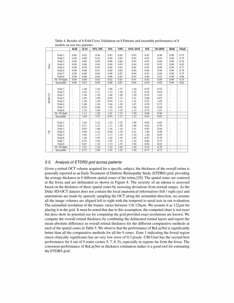
Table 4. Results of 8-Fold Cross Validation on 8 Patients and ensemble performance of 8models on rest two patients.

RaR ILM NFL-IPL INL OPL ONL-ISM ISE OS-RPE RbR FluidDice

Fold 1 0.99 0.92 0.94 0.87 0.85 0.93 0.92 0.90 0.99 0.75Fold 2 0.99 0.89 0.93 0.85 0.85 0.92 0.91 0.91 0.99 0.75Fold 3 0.99 0.89 0.95 0.88 0.84 0.93 0.93 0.89 0.99 0.76Fold 4 0.99 0.88 0.94 0.89 0.83 0.94 0.92 0.92 0.99 0.83Fold 5 0.99 0.95 0.95 0.88 0.83 0.91 0.93 0.89 0.99 0.77Fold 6 0.99 0.88 0.91 0.84 0.84 0.94 0.90 0.90 0.99 0.79Fold 7 0.99 0.89 0.94 0.88 0.87 0.94 0.93 0.89 0.99 0.75Fold 8 0.99 0.88 0.94 0.86 0.85 0.93 0.94 0.92 0.99 0.86

50 -50 Split 0.99 0.88 0.92 0.82 0.81 0.91 0.92 0.89 0.99 0.75Ensemble 0.99 0.91 0.95 0.88 0.87 0.94 0.94 0.92 0.99 0.81

MAD-LT

Fold 1 - 1.40 1.43 1.05 1.37 1.44 0.53 0.52 - -Fold 2 - 1.65 1.21 1.13 1.20 1.25 0.76 0.63 - -Fold 3 - 1.44 1.19 1.09 1.28 1.30 0.55 1.02 - -Fold 4 - 1.65 1.09 0.94 1.14 1.21 0.66 0.83 - -Fold 5 - 1.58 1.28 0.94 1.11 1.31 0.53 1.05 - -Fold 6 - 1.00 1.26 1.04 1.18 1.47 0.59 0.73 - -Fold 7 - 0.94 0.80 1.05 0.92 1.04 0.62 0.94 - -Fold 8 - 1.32 1.05 1.15 1.15 1.13 0.72 1.07 - -

50 -50 Split - 1.11 1.20 1.01 1.33 1.50 0.68 0.96 - -Ensemble - 1.04 1.07 0.93 1.17 1.12 0.63 0.85 - -

CE

Fold 1 - 1.05 1.12 1.25 1.25 1.99 0.92 0.82 - -Fold 2 - 0.71 1.31 1.11 1.28 1.98 0.83 0.76 - -Fold 3 - 0.83 1.06 1.16 1.16 1.41 0.85 0.94 - -Fold 4 - 0.99 1.12 0.84 1.39 2.21 1.00 0.90 - -Fold 5 - 1.05 1.17 1.17 1.34 1.19 1.20 0.85 - -Fold 6 - 1.04 1.07 1.02 1.45 1.03 0.87 0.79 - -Fold 7 - 0.76 1.02 1.07 1.16 1.18 0.86 0.73 - -Fold 8 - 0.87 1.18 1.15 1.35 1.94 0.94 0.82 - -

50 -50 Split - 1.01 1.16 1.32 1.45 1.94 0.74 0.78 - -Ensemble - 0.75 1.09 1.07 1.25 1.39 0.77 0.73 - -

5.5. Analysis of ETDRS grid across patients

Given a retinal OCT volume acquired for a specific subject, the thickness of the overall retina isgenerally reported as an Early Treatment of Diabetic Retinopathy Study (ETDRS) grid, providingthe average thickness in 9 different spatial zones of the retina [29]. The spatial zones are centeredat the fovea and are delineated as shown in Figure 8. The severity of an edema is assessedbased on the thickness of these spatial zones by assessing deviations from normal ranges. As theDuke SD-OCT dataset does not contain the local anatomical information (left / right eye) andannotations are made by sparsely sampling the OCT along the azimuthal direction, we assumeall the image volumes are aligned left to right with the temporal to nasal axis in our evaluation.The azimuthal resolution of the frames varies between 118-128µm. We assume it as 122µm forplacing it in the grid. It must be noted that due to this assumption, the computed chart is not exactbut does show its potential use for computing the grid provided exact resolutions are known. Wecompute the overall retinal thickness by combining the delineated retinal layers and report themean absolute difference in overall retinal thickness for the different comparative methods ateach of the spatial zones in Table 5. We observe that the performance of ReLayNet is significantlybetter than all the comparative methods for all the 9 zones. Zone 1 indicating the foveal region(most clinically significant) has an very low error of 0.3 pixels. CM-Unet has the second bestperformance for 4 out of 9 zones (zones 5, 7, 8, 9), especially in regions far from the fovea. Theconsistent performance of ReLayNet in thickness estimation makes it a good tool for estimatingthe ETDRS grid.

Zone 1

Zone 2

Zone 4

Zone 5 Zone 3

Zone 6(Superior)

Zone 7(Temporal)

Zone 8(Inferior)

Zone 9(Nasal)

Zone 9 Zone 6 Zone 2 Zone 6 Zone 7

(a) ETDRS Grid with 3 concentric circle with radius 1mm, 3mm and 5mm

(b) Sample B-scan OCT with the zones

Fig. 8. Illustration of ETDRS grid with 9 zones as demarcated in (a). This representsthe top view for a retinal OCT volume scan. A sample cross-sectional OCT B-scan slicecorresponding to the red line in the ETDRS grid is shown in (b). The different regions of theB-scan corresponding to the different zones are indicating by yellow lines in (b).

Table 5. Difference in retinal overall thickness (in pixels) for 9 zones in ETDRS grid acrosstesting subjects. The best performance is shown by bold, the second best is shown by ? andthe worst shown by †.

Zone 1 Zone 2 Zone 3 Zone 4 Zone 5 Zone 6 Zone 7 Zone 8 Zone 9Proposed 0.34 0.202 0.161 0.204 0.151 0.127 0.123 0.132 0.160CM-GDP 0.59 0.273 0.818† 0.375 0.698 0.889† 1.726† 0.849 2.565CM-KR 1.77† 0.231 0.474 0.986† 1.252† 0.820 1.050 0.965† 2.576†CM-LSE 0.64 0.230? 0.798 0.289? 0.803 0.775 1.189 0.471 2.036CM-Unet 0.89 0.468† 0.434 0.500 0.368? 0.325 0.340? 0.327? 0.378?CM-FCN 0.54? 0.405 0.398? 0.749 0.441 0.214? 0.443 0.797 0.461

6. Conclusion

In this paper, we have proposed ReLayNet, an end-to-end fully convolutional framework forsemantic segmentation of retinal OCT B-scan into 7 retinal layers and fluid masses. We train andvalidate it on a publicly available benchmark of expert annotated OCT B-scans acquired from10 patients. The training of ReLayNet involves minimization of a combined loss comprisingof weighted logistic loss and dice loss. ReLayNet is particularly suited for clinical applicationsowing to its improved test time in the order of 0.01 seconds to segment a single B-Scan.The proposed ReLayNet framework has been compared and validated against five state-of-

the-art retinal layer segmentation methods including ones using graph-based dynamic program-ming [13,15,20] and deep learning [17,19]. Additionally, comparisons have been reported againsteight incremental baselines validating each of the individual contributions. The evaluation wasperformed on the basis of three standard metrics including dice loss, retinal thickness estimationand deviation from layer contours. We demonstrate conclusively that ReLayNet exhibits superiorperformance in these comparisons and affirm that it can reliably segment even in the presence ofa high degree of pathology which severely affects the normal layered structure of the retina. Openquestions for future investigation include extension of ReLayNet into intra-operative scenarioslike retinal microsurgeries, which poses challenges of poor spatial resolution and artifacts inducedby surgical tools. With increasing training data, one could potentially introduce 3D convolutionalkernels to improve inter-frame consistency in volume segmentation.

Acknowledgements

This work was supported in part by the Faculty of Medicine at LMU (FöFoLe), the Bavarian StateMinistry of Education, Science and the Arts in the framework of the Centre Digitisation.Bavaria(ZD.B) and we thank the NVIDIA corporation for GPU donation.