Regulating a manager whose empire-building

preferences are private information?

Ana Pinto Borges

NIDISAG - Nucleo de Investigacao do Instituto Superior de Administracao e Gestao

Joao Correia-da-Silva

CEF.UP and Faculdade de Economia, Universidade do Porto.

Didier Laussel

Aix Marseille Univ (AMSE).

Abstract. We obtain the optimal contract for the government (principal) to regulate a

manager (agent) who has a taste for empire-building that is his/her private information.

This taste for empire-building is modeled as a utility premium that is proportional to the

difference between the contracted output and a reference output. We find that output

is distorted upward when the manager’s taste for running large firms is weak, downward

when it is strong, and equals a reference output when it is intermediate (in this case, the

participation constraint is binding). We also obtain an endogenous reference output (equal

to the expected output, which depends on the reference output), and find that the response

of output to cost is null in the short-run (in which the reference output is fixed), whenever

the manager’s type is in the intermediate range, and negative in the long-run (after the

adjustment of the reference output to equal expected output).

Keywords: Procurement, Regulation, Adverse selection, Empire-building, Reservation utility.

JEL Classification Numbers: D82, H42, H51, I11.

We are grateful to Ines Macho-Stadler, David Perez-Castrillo and two anonymous referees for very useful comments and

suggestions, and we thank participants in the 2009 SAET Conference and the 3rd Economic Theory Workshop in Vigo. Ana

Pinto Borges (anaborges@isag.pt) and Joao Correia-da-Silva (joao@fep.up.pt) thank Fundacao para a Ciencia e Tecnologia and

FEDER for financial support (research grants PTDC/EGE-ECO/114881/2009 and PTDC/EGE-ECO/111811/2009).

Corresponding author: Didier Laussel (didier.laussel@univ-amu.fr), Aix-Marseille Universite, GREQAM-CNRS, Chateau La-

farge, Route des Milles, 13290 Les Milles, France.

1

1 Introduction

Behavior of managers within firms is more complex than profit maximization.1 Its immediate

determinants include: salary, security, status, power, prestige, social service and professional

excellence (Niskanen, 1971; Brehm and Gates, 1997; Prendergast, 2007). An observed will-

ingness to manage a firm without significant monetary incentives should be attributed to

these non-monetary factors (Wilson, 1989).

The motivations of managers were synthesized and formalized by Williamson (1974), who

concluded that, in addition to a preference for profit, managers also display a preference

for expenses in staff and emoluments. Such preference for expenditure may accentuate

the business cycle, by inducing a systematic accumulation of staff and emoluments during

prosperity, with divestment frequently becoming necessary during adversity.

The empire-building motive is well documented (Donaldson, 1984), and has been emphasized

by Jensen (1986, 1993) as an origin of excess investment and output: “Managers have

incentives to cause their firms to grow beyond the optimal size. Growth increases managers’

power by increasing the resources under their control.”

Nevertheless, this tendency of managers towards empire-building has not been accounted

for in the standard theory of regulation under asymmetric information (Baron and Myerson,

1982; Guesnerie and Laffont, 1984; Maskin and Riley, 1984; Laffont and Tirole, 1986). There,

it is assumed that the managers’ objective is the maximization of the monetary transfers

that they receive, net of the monetary value of the effort that they exert. We believe that

extending the theory of regulation to incorporate the empire-building bias of managers will

have a positive effect on the design of procurement contracts. Recently, Borges and Correia-

da-Silva (2011) contributed in this direction, by extending the model of Laffont and Tirole

(1986) to allow the manager of the firm to have a tendency for empire-building, modeled as

a preference for high output.2

The intrinsic difficulty in the observation of managers’ preferences motivates us to pursue

this line of research by studying the case in which the empire-building preference of the

1Empirical evidence of deviations from profit-maximization was provided by Chetty and Saez (2005) andby Brown, Liang and Weisbenner (2007), who studied the response of corporations to the 2003 dividend taxcut in the USA.

2The preference for high output is related to the preference for staff considered by Williamson (1974).

2

manager is unobservable by the government. In this paper, we consider a model in which

the government (principal) offers a contract to a manager (agent) that has an unobservable

preference for high output.3 The model can be straightforwardly adapted to deal with the

case of firm’ owners offering a contract to a manager.

We model the preference for empire-building as a utility premium that is proportional to the

difference between the contracted output and a reference output (it will actually be a utility

penalty whenever the contracted output is lower than the reference output). The immediate

effect of this bias is that the manager becomes willing to accept a lower payment if the

contracted output is relatively high, and will demand a greater payment if it is relatively

low. The government has, therefore, reasons to prefer facing a manager with a strong

tendency for empire-building (as long as the optimal contract stipulates an output level that

is greater than the reference output).

In the case of complete information, we find that the contracted output is a strictly in-

creasing function of the observed manager’s preference for empire-building. There are two

mechanisms that generate this unsurprising result. One is the fact that when this prefer-

ence is stronger, the social marginal utility of output is greater. The other is related to the

compensation scheme. The government can reward the manager by increasing output or by

increasing the monetary transfer. When the preference for empire-building is stronger, the

increase in output that is needed to substitute a monetary reward becomes lower.

If the contracted output is lower (resp. higher) than the reference output, then a stronger

preference for empire-building implies a greater utility penalty (resp. premium) and, there-

fore, an increase (resp. a decrease) of the net monetary reward that the manager requires to

participate. In this case, the manager has incentives to overstate (resp. understate) his/her

taste for empire-building. Therefore, it may happen that managers with a strong preference

for empire-building (sufficiently strong for the contracted output to be higher than the refer-

ence output) tend to understate their preference, while managers with a weak preference for

empire-building (sufficiently weak for the contracted output to be lower than the reference

output) tend to overstate their preference. There are countervailing incentives (Lewis and

Sappington, 1989; Maggi and Rodriguez-Clare, 1995; Jullien, 2000; Laffont and Martimort,

2002).

3More precisely, the government offers an incentive compatible set of contracts, one for each possible typeof manager.

3

The tendency of managers to annouce an intermediate level of their preference for output

implies that: (i) the output of the extreme types is not distorted (because the other types do

not tend to mimic them); (ii) output is distorted below the perfect information level for high

types (this removes the manager’s incentives to understate their type, because the utility

premium would decrease); (iii) output is distorted above the perfect information level for

low types (this removes the manager’s incentives to overstate their type, because the utility

penalty would increase); (iv) output is at its reference level for a bunch of intermediate

types (this also removes the manager’s incentives to misrepresent their type, because the

attainable utility would remain equal to the reservation utility).

The reference output can be seen as a typical output level, that the manager associates with

neither a utility premium nor a utility penalty. It may be natural to keep the reference output

fixed when we estimate the short-run effects of an exogenous shock. But it is equally natural

to consider an endogenous reference output, which may adjust in response to exogenous

shocks, especially if we are interested in estimating the long-run effects of these shocks. We

also address this possibility, by making the reference output equal to the expected output

with respect to the probability distribution of manager’s types (notice that this expected

output depends on the reference output itself).

The consideration of an endogenous reference output is useful to improve our understanding

of the response of output to a change in the production cost. For example, in the case of

managers that have an intermediate taste for empire-building, the fact that the contracted

output is equal to the reference output implies that the cost-sensitivity of output is driven by

the adjustment of the reference output. Therefore: in the short-run (in which the reference

output is fixed), output does not respond to small variations in cost (remains equal to the

reference output); while in the long-run (after the adjustment of the reference output to

equal the expected output), the sensitivity of output to cost becomes negative (being driven

by the adjustment of the reference output).

We believe that we are pioneer in assuming the existence of private information about the

preference for empire-building. But, of course, we are not the first to investigate the economic

effects of deviations from profit-maximizing behavior. The early managerial discretion mod-

els (Baumol, 1959; Marris, 1963; Williamson, 1974) aimed to investigate the implications

of various hypotheses concerning the objective functions of managers, explicitly recognizing

that these may not coincide with profit-maximization. Baumol (1959) argued that some

firms maximize sales subject to a profit constraint, thus producing more than if they oper-

4

ated as profit-maximizers. These firms respond to external shocks in a very different way.

For example, if there is an increase in fixed costs or if a lump-sum tax is imposed, a firm

whose managers have a preference for staff will reduce its output, staff employment and

other perquisites.

A recent strand of literature is taking into account the preference of managers for empire-

building.4 The focus in this literature has been to develop models of financial structure based

on the desire to curb management’s empire-building tendencies, assuming that firms are

owned by shareholders who don’t observe cash-flows or investment decisions. The empire-

building bias is typically incorporated by assuming managerial private benefits of control

(Grossman and Hart, 1988) that are either proportional to investment (Hart and Moore,

1995; Zwiebel, 1996) or to the gross output from investment (Stulz, 1990).

It is worthwhile to compare our results with those of the early managerial discretion models

and of the models of optimal financial structure. Our result that output is an increasing func-

tion of the manager’s preference for output is in line with managerial discretion theory, but

results from a quite different mechanism. Instead of being the straightforward implication

of managerial discretion over output, it follows from the manager’s participation constraint:

a larger output yields a larger utility to the manager who, then, becomes willing to accept

a lower monetary transfer. Our result differs, however, from those in the above-mentioned

literature on optimal financial structure, where empire-building tendencies do not neces-

sarily lead to an empirical prediction of overinvestment (or overproduction) on average.5

Relatively to the sensitivity of output to cost, we find that, unlike what is predicted by

managerial discretion models, increases in marginal cost may have no effect on output (as

long as the reference output is kept fixed).

The paper is organized as follows. Section 2 describes the model and section 3 analyzes

the benchmark case of complete information. In section 4, we derive the optimal incentive

scheme and provide the general results. Section 5 presents an illustration for quadratic social

value functions and an uniform distribution over types (with an exogenous reference output

4See, for example, the works of Stulz (1990), Hart and Moore (1995), Harris and Raviv (1996), Li and Li(1996), Zwiebel (1996), Arya, Baldenius and Glover (1999) and Kanniainen (2000).

5Stulz (1990), Hart and Moore (1995) and Li and Li (1996) concluded that there is overinvestmentwhen the free cash-flow from previous investments is higher than expected, and underinvestment when itis lower. Assuming that managers have private information about productivity, Harris and Raviv (1996)concluded that there is underinvestment when productivity is higher than expected and overinvestment whenproductivity it is lower.

5

and with an endogenous reference output). Finally, section 6 offers some concluding remarks.

2 The model

We consider a model of procurement in which the government (principal) delegates to a firm

(agent) the provision of a public good. The manager of the firm cares about profit, t, but

also about the output level, q. The manager’s utility function is:

U = t+ δ (q − qref ) ,

where δ, the marginal utility of output to the manager, is a private information parameter,

drawn according to a probability distribution over an interval[δ, δ]∈ IR+, with strictly

positive density, f(δ) > 0, and monotone hazard rates, ddδ

[f(δ)

1−F (δ)

]> 0 and d

dδ

[f(δ)F (δ)

]< 0

(where F (δ) denotes the cumulative distribution function). The reference output, qref ≥ 0,

is independent of δ and may be interpreted as a “normal” output, such that producing this

output neither implies a utility increase nor a utility penalty.6

The manager accepts to participate if and only if U(δ) ≥ 0, ∀δ ∈[δ, δ].

The production cost is βq, where the marginal cost, β > 0, is observable by the government.

The social value of output is S(q), with marginal social value being strictly positive and

decreasing, S ′(q) > 0 and S ′′(q) < 0, for any q ∈ [0, q). We also set S(0) = 0 and S ′(q) = 0

(where q can be interpreted as fully covering the needs of the population).

The government finances public good provision using a distortionary mechanism (taxes, for

example), so that the social cost of raising one unit of money is 1+λ, with λ > 0. The welfare

of consumers is the difference between the social value of the public good and the cost of

financing its provision, S(q)−(1+λ)(t+βq). In the model of Laffont and Tirole (1986, 1993)

and, more generally, in the regulation literature, the government is assumed to maximize

the sum of the consumers’ welfare with the utility of the firm. With the incorporation of an

empire-building tendency, it becomes natural to consider two possibilities:

(i) social welfare, W (δ), is the sum of the consumer’s welfare with the utility of the firm

(this case corresponds to setting k = 0, below);

(ii) social welfare, W (δ), is the sum of the consumer’s welfare with the profit of the firm,

6In section 5.2, we propose an endogenous determination of this reference level of output.

6

while the empire-building component of the manager’s utility is excluded (corresponds to

setting k = 1, below).7

The problem of the government (maximization of expected social welfare) is:

maxq,t

∫ δ

δ

[S(q)− (1 + λ)(t+ βq) + U − kδ(q − qref )] f(δ) dδ

subject to

U ≥ 0.

3 The case of complete information

As a benchmark, we study the case in which there is no asymmetry of information between

the government and the firm (the government is able to observe δ).

The problem of the government can be written as:

maxq,U{S(q)− (1 + λ) βq − λU + (1 + λ− k) δ (q − qref )}

subject to

U ≥ 0.

We make the following assumptions, similar to those in Laffont and Tirole (1986), for the

problem to be well-behaved.

Assumption 1.

(i) λ > 0;

(ii) ∀q ∈ [0, q) , S ′′(q) < 0;

(iii) S ′(0) > (1 + λ) (β − δ) + kδ;

(iv) β > 1+λ−k1+λ

δ.

Under Assumption 1: (i) guarantees that the participation constraint is binding, (ii) ensures

7We also allow for intermediate cases, i.e., any k ∈ (0, 1).

7

that the second order condition is satisfied, (iii) ensures a positive output level, and (iv) is

necessary for the equilibrium output to be lower than q.

With λ > 0, the objective function is strictly decreasing in U , therefore the participation

constraint is binding. We can replace U = 0 in the objective function and then solve for q.

The corresponding first-order condition is:

S ′(q) = (1 + λ) (β − δ) + kδ. (1)

And the second order condition is: S ′′(q) < 0 (always satisfied).

Since the participation constraint is binding: the utility level of the manager is U∗c (δ) = 0;

and the net transfer is:

t∗c(δ) = δ [qref − q∗c (δ)] .

Observe that the net monetary transfer from the government to the firm, t∗c , is positive if and

only if the output, q∗c , is lower than the reference output, qref (because we have normalized

the reservation utility to zero).8

The optimality condition (1) equates the marginal benefit of output to consumers, S ′(q),

and the social marginal cost. Using this condition, the optimal output level, q∗c , can be

obtained. It is clear that when the regulator cares about the non-monetary component of

the manager’s utility (k = 0), the level of output is higher and the net monetary transfer

is lower than when it does not care (k = 1). Observe also that the optimal output level is

an increasing function of the preference for output parameter, even when the regulator does

not care at all about the utility that the manager derives from output (k = 1). This occurs

because increasing the output implies an increase in the non-monetary component of the

manager’s utility, decreasing, therefore, the monetary transfer which is necessary to induce

participation.

We also find that the social welfare is increasing (resp. decreasing) with the intensity of the

empire-building preference, δ, if and only if the optimal output, q∗c , is higher (resp. lower)

8In some circumstances, managers may be willing to pay a fraction of the production costs, as in somevolunteering activities or internships.

8

than the reference output, qref . Applying the Envelope Theorem:

dW ∗c

dδ=∂W ∗

c

∂δ= (1 + λ− k) (q∗c − qref ) .

Since q∗c is increasing in δ, we conclude that social welfare, W ∗c , is a convex function of δ:

d2W ∗c

dδ2> 0.

In the following section, we determine the optimal procurement contract in the presence of

an unobservable tendency for empire-building.

4 The optimal incentive scheme

In the asymmetric information case, the government does not know the manager’s marginal

utility of output, δ. At the moment of contracting, the government only knows the prior

probability distribution of δ.

Thanks to the Revelation Principle, we can restrict (without loss of generality) our attention

to incentive compatible direct revelation mechanisms.9

The timing of the game is the following:

(1) nature chooses the preference for output of the manager, δ ∈[δ, δ];

(2) the government offers a contract to the manager, [q(δ), t(δ)], specifying a level of

output and a net payment that depend on the preference for output that is announced by

the manager, δ;

(3) the manager either accepts the contract, announces a type, δ, produces q(δ) and

receives the net transfer t(δ), or rejects the contract and receives a null payoff.

In this section, we will consider that if the manager rejects the contract, the government

receives a large negative payoff. The government is, therefore, forced to participate.10

9By the revelation principle (Myerson, 1979), given a Bayesian Nash equilibrium of a game of incompleteinformation, there exists a direct mechanism that has an equivalent equilibrium where the players truthfullyreport their types. A direct-revelation mechanism is said to be incentive compatible if, when each individualis expecting the others to be truthful, then he/she has interest in being truthful.

10In the light of Proposition 6, it will be clear that the government obtains a positive payoff for all types

9

4.1 The firms’s optimization problem

The government offers a contract to the manager such that he/she receives a net transfer

t(δ) for producing the contracted output level q(δ), and has to pay an extreme penalty,

t(δ) = −∞, if the output level turns out to be different from q(δ).

For any δ ∈[δ, δ], truthful revelation must maximize the utility of the manager:

δ ∈ arg maxδ∈[δ,δ]

{t(δ) + δ

[q(δ)− qref

]}. (2)

Let V (δ) be the manager’s value function (attainable utility as a function of δ):

V (δ) = maxδ∈[δ,δ]

{t(δ) + δ

[q(δ)− qref

]}= t(δ) + δ [q(δ)− qref ] .

If announcing δ 6= δ is not optimal (2), then the output, transfer and value functions are

almost everywhere differentiable (see Appendix A.1.1).

The first-order condition of (2) implies that the output and transfer functions vary in opposite

directions:

t′(δ) + δq′(δ) = 0. (3)

From the Envelope Theorem, we obtain the first-order incentive compatibility constraint:

V ′(δ) = q(δ)− qref , (4)

which tells us that the derivative of the value function with respect to δ is equal to the

difference between the output level and the reference output.

The second-order incentive compatibility constraint is derived from the second-order condi-

tion of utility maximization (see Appendix A.1.2):11

q′(δ) ≥ 0. (5)

δ ∈[δ, δ]

if and only if the reference output, qref , is below a certain threshold.

11In Appendix A.1.3 we show that the first-order and second-order incentive compatibility constraints, (4)and (5), are equivalent to truth-telling (2).

10

It implies that the output level is non-decreasing with the manager’s preference for output.

Thus, from (3), the net transfer is non-increasing.

4.2 The government’s optimization problem

The objective of the government is to maximize expected social welfare, Eδ [W (δ)]:

maxq(δ),V (δ)

∫ δ

δ

{S [q(δ)]− (1 + λ)βq(δ)− λV (δ) + (1 + λ− k) δ [q(δ)− qref ]} f(δ) dδ, (6)

subject to, ∀δ ∈[δ, δ], the incentive conditions (4) and (5), and the participation constraint

V (δ) ≥ 0.

Observe that the incentive compatibility conditions, (4) and (5), imply that V (δ) is a convex

function. Therefore, the participation constraint is binding over an interval, that we denote

by [δ0, δ1], with δ ≤ δ0 ≤ δ1 ≤ δ.12

The following characterization is a strightforward consequence of the incentive compatibility

conditions.

Proposition 1 (Level of output and sign of net transfer).

The participation constraint, V (δ) ≥ 0, binds at [δ0, δ1], where δ ≤ δ0 ≤ δ1 ≤ δ.

(i) For δ < δ0, the output is lower than the reference output, q(δ) < qref , and the monetary

transfer is positive, t(δ) > 0;

(ii) For δ0 ≤ δ ≤ δ1, the output is equal to the reference output, q(δ) = qref , and the

monetary transfer is null, t(δ) = 0;

(iii) For δ > δ1, the output is higher than the reference output, q(δ) > qref , and the

monetary transfer is negative, t(δ) < 0.

Proof. See Appendix A.2.

12This includes, for example, the case in which the participation constraint is only binding at one of theextremes of the interval (δ0 = δ1 = δ or δ0 = δ1 = δ).

11

To further characterize the solution, we start by solving a relaxed problem in which condition

(5) is ignored (Appendix A.3.1). Then, we check that the solution of this relaxed problem

is the solution of the general problem (Appendix A.3.2).

Proposition 2 (Behavior of output and net transfer).

The behavior of output and net transfer is such that:

(i) For δ < δ0, the output is distorted upwards, q(δ) > q∗c (δ), and strictly increasing,

q′(δ) > 0, and the monetary transfer is positive, t(δ) > 0 and strictly decreasing, t′(δ) < 0;

(ii) For δ0 ≤ δ ≤ δ1, the output is constant and equal to the reference output, q(δ) = qref ,

and the monetary transfer is also constant, t(δ) = 0;

(iii) For δ > δ1, the output is distorted downwards, q(δ) < q∗c (δ), and strictly decreasing,

q′(δ) < 0, and the monetary transfer is negative, t(δ) < 0, and strictly increasing, t′(δ) > 0.

Proof. See Appendix A.3.

The distortion of output results, obviously, from the need to induce truth-telling. If the

manager happens to have a relatively strong preference for high output, contracted output

is below the perfect information level. This means that it would be preferable to “pay” more

in output and less in money. But in this range the principal must avoid that the higher

types mimic the lower. Paying more in output to type δ would make it even more costly to

prevent type δ + ε from mimicking type δ. Of course that this argument no longer holds at

δ = δ, and this is why distortion disappears for the highest type (see Figures 1, 2 and 3 in

the next section).

5 Characterizing the optimal contract

In this section, we characterize the optimal contract in the case of a quadratic social value

function of output and a uniform distribution over types.

12

5.1 Exogenous reference output

In order to illustrate our general results, we now assume that the social value of output is

S(q) = αq − 12q2 and that δ is uniformly distributed on [0, 1].

With complete information, the solution is:

q∗c (δ) = α− (1 + λ)β + (1 + λ− k)δ,

t∗c(δ) = δ [qref − q∗c (δ)] .

Assumption 1 (iii), which in this case is α > (1+λ)β, ensures that the complete information

output is always positive.

We have bunching if and only if the reference output is not too large nor too small. Pre-

cisely, assuming that qref ∈ [α− (1 + λ)β − λ, α− (1 + λ)β + 1 + 2λ− k], the participation

constraint binds in the interval δ ∈ [δ0, δ1], where (see Appendix A.4.1):

δ0 = max

{0,qref − α + (1 + λ)β

1 + 2λ− k

}and δ1 = min

{qref − α + (1 + λ)β + λ

1 + 2λ− k, 1

}. (7)

Without the above restriction on the value of the reference output, we obtain: δ0 > 1 (if

qref > α − (1 + λ)β + 1 + 2λ− k), meaning that the participation constraint only binds at

δ = 1; or δ1 < 0 (if qref < α− (1 + λ)β − λ), meaning that it only binds at δ = 0.

The analytical expressions for output, net transfer and manager’s utility are presented in

Appendices A.4.2 and A.4.3.

Qualitatively, the solution is characterized by the following propositions.

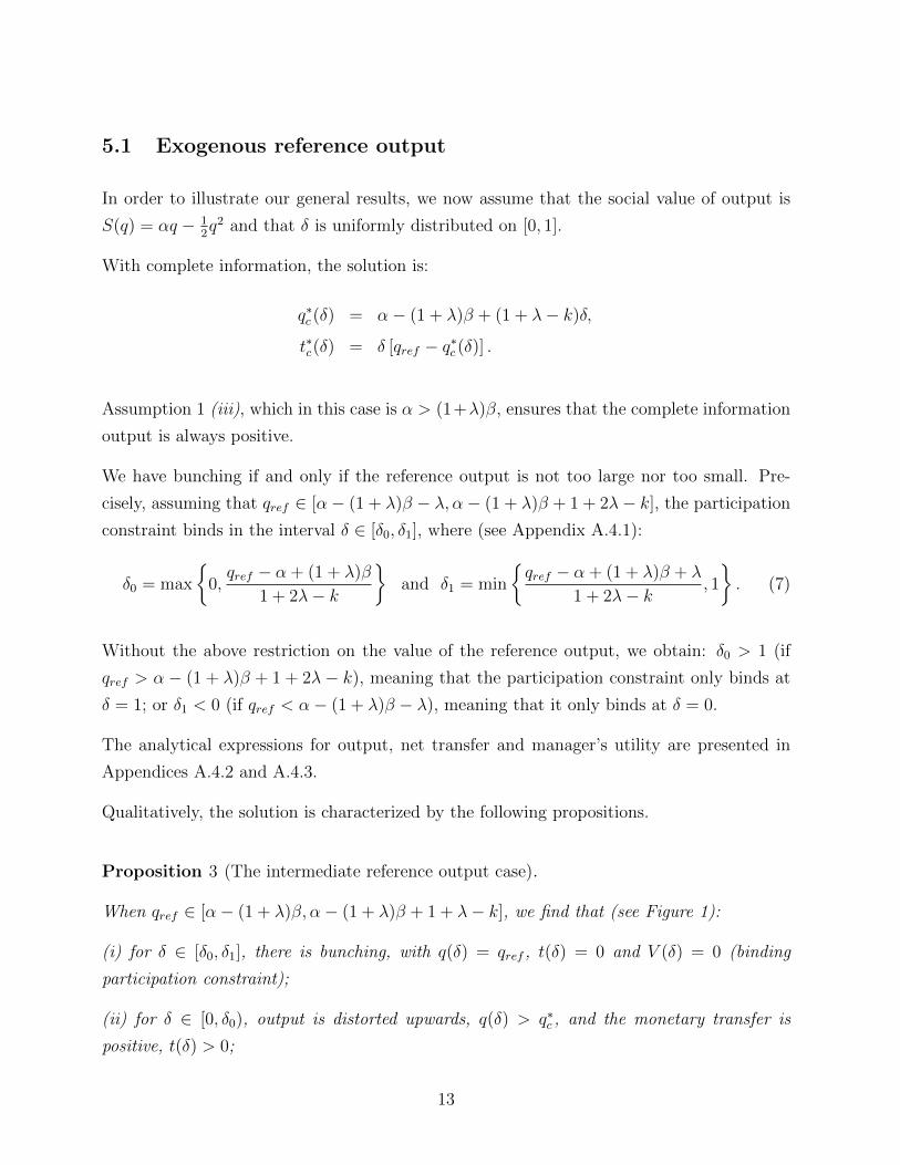
Proposition 3 (The intermediate reference output case).

When qref ∈ [α− (1 + λ)β, α− (1 + λ)β + 1 + λ− k], we find that (see Figure 1):

(i) for δ ∈ [δ0, δ1], there is bunching, with q(δ) = qref , t(δ) = 0 and V (δ) = 0 (binding

participation constraint);

(ii) for δ ∈ [0, δ0), output is distorted upwards, q(δ) > q∗c , and the monetary transfer is

positive, t(δ) > 0;

13

(iii) for δ ∈ (δ1, 1], output is distorted downwards (q(δ) < q∗c ) and the monetary transfer is

negative, t(δ) < 0.

Proof. See Appendices A.4.2 and A.4.3.

When δ increases from 0 to 1, the output level first increases (until δ0), being larger than

the complete information output, then it is constant (between δ0 and δ1), and then increases

again, being lower than the complete information optimal output.

The intermediate reference output case

Figure 1: Output and utility of the manager with k = 0, α = 3, λ = 0.5, β = 1.2 and qref = 1.5.

The following propositions describe what happens when the reference output qref is outside

the interval defined in Proposition 3.

Proposition 4 (The large reference output case).

When qref ∈ (α− (1 + λ)β + 1 + λ− k, α− (1 + λ)β + 1 + 2λ− k), there is bunching at the

top (see Figure 2):

(i) for δ ∈ [δ0, 1], there is bunching, with q(δ) = qref , t(δ) = 0 and V (δ) = 0 (binding

participation constraint);

(ii) for δ ∈ [0, δ0), output is distorted upwards, q(δ) > q∗c , and the monetary transfer is

positive, t(δ) > 0.

14

Proof. See Appendix A.4.2.

The large reference output case

Figure 2: Output and utility of the manager with k = 0, α = 3, λ = 0.5, β = 1.2 and qref = 2.8.

Proposition 5 (The small reference output case).

When qref ∈ (α− (1 + λ)β − λ, α− (1 + λ)β), there is bunching at the bottom (see Figure

3):

(i) for δ ∈ [0, δ1], there is bunching, with q(δ) = qref , t(δ) = 0 and V (δ) = 0 (binding

participation constraint);

(ii) for δ ∈ (δ1, 1], output is distorted downwards, q(δ) < q∗c , and the monetary transfer is

negative, t(δ) < 0.

Proof. See Appendix A.4.3.

The figures illustrate the case in which the government incorporates the non-monetary com-

ponent of the manager’s utility in the welfare function (k = 0). If the government does not

care about the preference for empire-building (k = 1), the interval over which the output is

constant and the participation constraint of the manager is binding moves to the right and,

outside this interval, the output and the manager’s utility are lower.

15

The small reference output case

Figure 3: Output and utility of the manager with k = 0, α = 3, λ = 0.5, β = 1.2 and qref = 1.1.

We can use our results to study how the output responds to changes in cost, for a given

reference output level. An increase in marginal cost, β, entails a reduction of the output level

both when the manager’s marginal utility is low (δ ∈ [0, δ0]) and when it is high (δ ∈ [δ1, 1]).

However, for intermediate values (δ ∈ [δ0, δ1]), output does not change in response to (small)

changes in cost.

Finally, we show that a sufficient condition for social welfare, W (δ), to be positive for all

δ ∈ [0, 1] (which implies that the regulator is happy to offer a contract to all possible types)

is that the reference output is not larger than twice the optimal output in the absence of

empire-building tendencies.

Proposition 6 (The government’s participation constraint).

If qref ≤ 2 [α− (1 + λ)β], then the social welfare is positive, W (δ) > 0, for all δ ∈ [0, 1].

Proof. See Appendix A.4.4.

In Figure 4, we observe that if the government cares about the managerial empire-building

utility (k = 0), the social welfare increases with δ. If the government disregards the manage-

rial empire-building utility in the welfare function (i.e., when k increases), the social welfare

increases in δ ∈ [0, δ0), is constant in δ ∈ [δ0, δ1], and increases again in δ ∈ (δ1, 1].

16

Social welfare with asymmetric information

Figure 4: Social welfare for k = 0 versus k = 1, with α = 3, λ = 0.5, β = 1.2, qref = 1.5.

5.2 Endogenous reference output

Until now, we considered that the reference output was exogenous. Suppose now that there

is a large population of symmetric principals that are randomly matched with a large pop-

ulation of managers that differ in their tendency for empire-building. If we consider that

the utility premium or penalty that is associated with the output level results from the

comparison between the manager’s output and the average output across the population of

managers (“keeping up with the Joneses”), then it is natural to assume that the reference

output is the expected output of the population of firms, with respect to the managers’

types.13 Since this expected value depends on the reference output itself, the equilibrium

value of the reference output is to be determined by stipulating that the reference output

should equal the expected output, qref = Eδ [q(δ)].

With an endogenous reference output, we cannot have a “large reference output” nor a

“small reference output”. An “intermediate reference output” must emerge because, for the

expected output to coincide with the reference output, if some managers produce less than

the reference output, other managers must produce more than the reference output.

13This is in the spirit of Koszegi and Rabin (2006), where the reference point of an agent corresponds tohis/her rational expectation about a certain outcome.

17

Proposition 7 (Endogenous reference output).

The endogenous reference output level is such that only the “intermediate reference output

case” occurs at equilibrium.

Proof. Suppose that we have an endogenously “large reference output”. Then, for δ ∈ [δ, δ0],

we have q(δ) < qref , while, for δ ∈[δ0, δ

], we have q(δ) = qref . Therefore, Eδ [q(δ)] < qref ,

which contradicts the hypothesis that qref is an endogenous reference output.

A similar argument applies to contradict the possibility of a “small reference output”.

With quadratic social value of output and a uniform distribution over types, whenever the

reference output is assumed to take an intermediate value, the expected output is given by:

Eδ [q(δ)] =

∫ δ0

0

[α− (1 + λ)β + (1 + 2λ− k)δ] dδ +

∫ δ1

δ0

qref dδ

+

∫ 1

δ1

[α− (1 + λ)β + (1 + 2λ− k)δ − λ] dδ. (8)

Equating (8) to qref , we obtain the unique equilibrium value of qref as:

q∗ref = α− (1 + λ)β +1

2(1 + λ− k). (9)

Observing that q∗ref ∈ [α− (1 + λ)β, α + (1 + λ)(1− β)− k], we validate, using Proposition

3, that the endogenous reference output takes an intermediate value.

The corresponding endogenous threshold values δ0 and δ1 are given by:

δ0 = max

{0,

1

2− λ

2(1 + 2λ− k)

}and δ1 = min

{1

2+

λ

2(1 + 2λ− k), 1

}. (10)

Making the reference output endogenous in this way leads us to reconsider what has been said

at the end of the previous section. It is true that, for a given reference output, the output may

not respond to “small” changes in cost when the managers’ types are intermediate. However,

the (endogenous) reference output itself will adjust in response to changes in cost. Then, it

makes sense to distinguish between short-run and long-run cost-elasticity of output. In the

short-run, the reference output is given, for instance because the contracts have already been

18

signed between the principals and the managers, and output can be insensitive to changes

in costs or taxes for a group of projects. However, in the long run, as the old managers

leave their jobs, new contracts are passed referring to the new reference output, and output

converges to its new equilibrium value. It follows that the elasticity of output with respect

to cost is going to be larger (in absolute value) in the long-run than in the short-run.

Proposition 8 (Cost-elasticity of output).

After an increase in the production cost (β), the output of the managers with low and high

preference for output (δ ≤ δ0 and δ ≥ δ1) decreases in the short-run and is not affected

by the subsequent adjustment of the reference output. On the other hand, the output of the

managers with an intermediate preference for output (δ0 ≤ δ ≤ δ1) remains unchanged in

the short-run and only decreases in the long-run.

Proof. See Appendix A.4.5.

Two remarks need to be made regarding the way the endogenous reference output was

determined.14 First, the endogenous reference output is related to the output decisions of

the principals. In a large world (with an infinite number of principals), the behaviour of an

individual principal has no effect on the average output level, and thus it is consistent to

assume that each principal takes qref as a given. However, this would not be the case in a

small world (with a finite number of principals). Second, the endogenous reference output

may be seen as being related to the reservation utility of the manager.15 If we assume that

the outside option of the manager is to remain unemployed, then it is reasonable to assume

that qref is independent of the manager’s tendency for empire-building. However, if the

outside option corresponded to managing an alternative project, possibly producing a type-

dependent output level, then qref should be considered to be type-dependent. We believe

that these two lines of investigation are of interest and leave them for future work.

14We thank two anonymous referees for pointing out these two issues.

15If we interpret the choice behavior of the managers as resulting from the objective function U = t+ δq,with participation requiring U ≥ δqref .

19

6 Concluding remarks and extensions

In this paper, we analyzed the optimal regulation of a firm when the manager’s empire-

building preference (manager’s utility of output) is private information and the reservation

utility is type-dependent. We showed that the optimal output function is such that output is

distorted upward when the manager has a low preference for output, downward when he/she

has a high preference for output and equals his/her reference output when he/she has an

intermediate preference for output (in this case, the participation constraint is binding).

These results have implications for the cost-sensitivity of output. In the short-run, when the

reference output can be considered as exogenous, the output of firms whose managers’ types

are intermediate are not going to respond to small variations in their unit cost of production,

while the output of firms whose managers’ types are either small or large will respond in

the expected direction.16 The overall sensitivity of output to cost variations depends on the

relative numerical importance of these three groups of firms, or, using the terminology of

this model, on the length of the interval [δ0, δ1]. In the long-run, the reference output adjusts

progressively to its new equilibrium level, and so the cost-elasticity of output is larger.

For the sake of simplicity, we assumed throughout this paper that the government can

observe the unit cost of production, and we simultaneously ignored the issue of moral hazard.

Analyzing a model where both the marginal cost and the manager’s utility for output are

private information would be fruitful. This will be the subject of future research.

16This looks like the result obtained by Sweezy (1939) in the very different framework of “the kinkedoligopoly demand curve”.

20

A Appendix

A.1 Incentive compatibility conditions

A.1.1 Differentiability of output, transfer, and utility functions

In this section, we prove that if (2) holds, then the output, transfer and value functions are

almost everywhere differentiable.

For simplicity of exposition, we will denote by U(δ, δ) the utility attained by a manager that

announces δ when his/her type is δ.

Claim 1. δ < δ ⇒ q(δ) ≤ q(δ).

Proof. If (2) holds, then:

t(δ) + δ [q(δ)− qref ] ≥ t(δ) + δ[q(δ)− qref

],

t(δ) + δ[q(δ)− qref

]≥ t(δ) + δ [q(δ)− qref ] .

Adding the two inequalities, we obtain:(δ − δ

) [q(δ)− q(δ)

]≥ 0.

Then, δ − δ > 0 implies that q(δ)− q(δ) ≥ 0.

Claim 2. U(δ, δ), as a function of δ, is nondecreasing on [δ, δ] and nonincreasing on[δ, δ].

Proof. Let us show monotonicity on [δ, δ]. Assume that δ < δ′ < δ and, by way of contra-

diction, U(δ, δ) > U(δ′, δ), that is:

t(δ) + δ[q(δ)− qref

]> t(δ′) + δ [q(δ′)− qref ] .

21

On the other hand, we know that a firm of type δ′ prefers to announce δ′ rather than

announce δ:

t(δ′) + δ′ [q(δ′)− qref ] ≥ t(δ) + δ′[q(δ)− qref

].

Adding the last two equations, we obtain:

(δ − δ′)[q(δ)− q(δ′)

]> 0 ⇒ q(δ)− q(δ′) > 0.

Which is in contradiction with Claim 1.

Monotonicity on[δ, δ]

can be proved in the same way.

Claims 1 and 2 imply that the functions q(δ) and t(δ) + δ′ [q(δ)− qref ] are a.e. differentiable.

Hence, t(δ) and V (δ) = t(δ) + δ [q(δ)− qref ] are also a.e. differentiable.

A.1.2 Second-order incentive compatibility condition

The local second-order condition of the maximization program is:

∂2U(δ, δ)

∂δ2

∣∣∣∣∣δ=δ

≤ 0 ⇔ t′′(δ) + δq′′(δ) ≤ 0. (11)

We want to show that (given the first-order condition) it is equivalent to q′(δ) ≥ 0.

Differentiating (3) with respect to δ, we obtain:

t′′(δ) + q′(δ) + δq′′(δ) = 0. (12)

Subtracting (12) from (11), the local second-order condition becomes: q′(δ) ≥ 0. �

22

A.1.3 The local second-order condition implies the global one

Claim 3. The first and second incentive compatibility conditions, (4) and (5), imply that

truth-telling is optimal (the local second-order condition implies the global one).

Proof. For δ > δ (a similar reasoning applies to δ < δ):

t(δ) + δ[q(δ)− qref

]= t(δ) +

∫ δ

δ

t′(γ)dγ + δ

[q(δ) +

∫ δ

δ

q′(γ)dγ − qref

]=

= t(δ) + δ [q(δ)− qref ] +

∫ δ

δ

t′(γ) + δq′(γ)dγ.

To finish the proof, it is only necessary to show that∫ δδt′(γ) + δq′(γ)dγ ≤ 0.

From the second-order condition, q′(γ) ≥ 0, it is clear that:

∫ δ

δ

t′(γ) + δq′(γ)dγ ≤∫ δ

δ

t′(γ) + γq′(γ)dγ.

The first-order condition, t′(γ) + γq′(γ) = 0, implies that∫ δδt′(γ) + γq′(γ)dγ = 0.

A.2 Level of output and sign of net transfer

In the interval in which the participation constraint is binding, we must have q(δ) = qref

and t(δ) = 0.

For δ < δ0, since q(δ) is non-decreasing and V (δ) > 0, we must have q(δ) < qref . It should

be clear that if q(δ) = qref , then q(δ′) = qref for all δ′ ∈ [δ, δ0], and, from (4), V (δ) = 0

(contradicting the fact that δ < δ0). Since q(δ) < qref , participation implies that t(δ) > 0.

Similarly, for δ > δ1, we must have q(δ) > qref . To avoid type δ1 from mimicking type δ, it

is necessary that t(δ) < 0. �

23

A.3 Problem of the government

We start by defining a relaxed problem in which the second-order incentive compatibility

condition (5) is ignored. After solving this relaxed problem, we will check that its solution

is also the solution of the general problem (6).

A.3.1 Solution of the relaxed problem

Consider a relaxed problem in which condition (5) is omitted.

Incorporating the participation constraint in the objective function, this relaxed problem

can be written as follows:17

maxq(δ),V (δ)

∫ δ

δ

{S [q(δ)]− (1 + λ)βq(δ)− λV (δ) + (1 + λ− k)δ [q(δ)− qref ]} f(δ) +

+η(δ)λV (δ) dδ, (13)

subject to, for all δ,

V ′(δ) = q(δ)− qref ,

where η(δ) satisfies η(δ) ≥ 0 and η(δ)λV (δ) = 0. Notice that η(δ)λ is the Lagrangian

multiplier associated to the participation constraint of type δ.18

Necessary conditions

The Hamiltonian is:

H = {S [q(δ)]− (1 + λ)βq(δ)− λV (δ) + (1 + λ− k)δ [q(δ)− qref ]} f(δ) +

+µ(δ)[q(δ)− qref ] + η(δ)λV (δ), (14)

where µ(δ) is the co-state variable associated with the incentive constraint (4).

17See Basov (2005), pages 124-126.

18The participation constraint must be binding for some δ, otherwise the government could increaseexpected social welfare by reducing the transfers to all types of managers without violating the participationand the incentive constraints.

24

The first-order conditions imply that:

µ′(δ) = λ [f(δ)− η(δ)] , (15a)

V ′(δ) = q(δ)− qref , (15b)

S ′ [q(δ)]− (1 + λ)(β − δ)− kδ +µ(δ)

f(δ)= 0, (15c)

η(δ)V (δ) = 0, (15d)

µ(δ) = µ(δ) = 0, (15e)

η(δ) ≥ 0, V (δ) ≥ 0. (15f)

Equation (15a) is the equation of motion of the co-state variable. Equation (15d) is the

complementary slackness condition. Equation (15e) gives the transversality conditions.

Let ζ(δ) =∫ δδη(s)ds. It is shown below that η is a probability distribution on

[δ, δ], and

that, therefore, ζ(δ) is a c.d.f. on[δ, δ].

Integrating equation (15a) we obtain:

µ(δ) = λ [F (δ)− ζ(δ)] , (16)

and using (15e):

µ(δ) = λ [F (δ)− ζ(δ)] ⇔ 0 = −λζ(δ) ⇔ ζ(δ) = 0,

µ(δ) = λ[F (δ)− ζ(δ)

]⇔ 0 = λ

[1− ζ(δ)

]⇔ ζ(δ) = 1.

These last two equations imply that:

∫ δ

δ

η(δ)dδ =

∫ δ

δ

f(δ)dδ = 1,

meaning that η(·) is a probability distribution on[δ, δ]

and ζ(·) is the corresponding c.d.f..

Replacing equation (16) into (15c), we find that output is such that:

S ′ [q(δ)]− (1 + λ)(β − δ)− kδ + λF (δ)− ζ(δ)

f(δ)= 0. (17)

25

The only difference with respect to the complete information case is the last term. It should

be clear that ζ(δ) = 1 implies downward distortion and ζ(δ) = 0 implies upward distortion.

Note that if the participation constraint (4) is not binding on some open interval, (δa, δb),

then ζ(·) is constant on it, since ζ ′(δ) = η(δ) = 0.

Sufficient condition

The second order derivative of the Hamiltonian (14) is: ∂2H∂q2

= S ′′ [q(δ)] < 0.

A.3.2 Solution of the general problem

We now check that the condition that was omitted in the relaxed problem (13), q′(δ) ≥ 0, is

satisfied. Differentiating equation (17) with respect to δ, we obtain:

q′(δ) = −1 + λ− k + λ

[1− η(δ)

f(δ)

]− λf

′(δ)[F (δ)−ζ(δ)]f(δ)2

S ′′[q(δ)].

The assumption of monotone hazard rates is used here. Observe that:

d

dδ

[f(δ)

F (δ)

]< 0 ⇔ f ′(δ)F (δ)

f(δ)2< 1

andd

dδ

[f(δ)

1− F (δ)

]> 0 ⇔ f ′(δ) [F (δ)− 1]

f(δ)2< 1.

For δ < δ0, we have η(δ) = 0 and ζ(δ) = 0, implying that:

q′(δ) = −1 + 2λ− k − λf

′(δ)F (δ)f(δ)2

S ′′[q(δ)]> −1 + λ− k

S ′′[q(δ)]> 0.

For δ > δ1, we have η(δ) = 0 and ζ(δ) = 1, implying that:

q′(δ) = −1 + 2λ− k − λf

′(δ)[F (δ)−1]f(δ)2

S ′′[q(δ)]> −1 + λ− k

S ′′[q(δ)]> 0.

When the participation constraint is binding, q(δ) = qref and, therefore, q′(δ) = 0. This

26

implies that (5) is verified. The solution of the unconstrained problem (13) is also the

solution of the general problem (6).

We also conclude that the output level is strictly increasing with δ over the two intervals

[δ, δ0] and[δ1, δ

], being constant and equal to qref in [δ0, δ1].

From (3), when the output level is strictly increasing, the monetary transfer, t(δ), is strictly

decreasing. �

A.3.3 Output distortions

If δ < δ0, then ζ(δ) = 0 and the output is such that:

S ′ [q(δ)] = (1 + λ)(β − δ) + kδ − λF (δ)

f(δ).

In the case of complete information, we had S ′ [q∗c (δ)] = (1 +λ)(β− δ) + kδ, which is greater

than S ′ [q(δ)]. Therefore, q(δ) > q∗c (δ).

If δ > δ1, then ζ(δ) = 1 and the output is such that:

S ′ [q(δ)] = (1 + λ)(β − δ) + kδ + λ1− F (δ)

f(δ).

With complete information, S ′ [q∗c (δ)] = (1 + λ)(β − δ) + kδ, which is smaller than S ′ [q(δ)].

Therefore, q(δ) < q∗c (δ). �

A.4 Quadratic social value and uniform distribution

Characterizing the optimal output level and the manager’s utility over the interval [δ0, δ1] is

straightforward. When δ ∈ [δ0, δ1], the participation constraint is binding: V (δ) = 0. From

the first incentive compatibility constraint (4), we have q(δ) = qref , ∀ δ ∈ [δ0, δ1].

Below, we obtain the values of δ0 and δ1 and we study the two intervals where the

participation constraint is not binding: δ ∈ [0, δ0) and δ ∈ (δ1, 1].

27

A.4.1 The values of δ0 and δ1

From (17), we know that:

ζ(δ) =1

λ[α− q(δ)− (1 + λ) β − kδ] +

(2 +

1

λ

)δ. (18)

Since ζ(0) = 0 and η(δ) = 0 for all δ < δ0, we must have ζ(δ0) = 0. Replacing in equation

(18) and using the fact that q(δ0) = qref , we obtain:

δ0 = max

{0,qref − α + (1 + λ)β

1 + 2λ− k

}. (19)

When qref > α − (1 + λ)β ≡ q∗(0), we obtain δ0 > 0, whereas, when qref ≤ α − (1 + λ)β,

bunching occurs at the bottom of the interval, i.e., δ0 = 0.

Since ζ(1) = 1 and η(δ) = 0 for all δ > δ1, it must be the case that ζ(δ1) = 1. Replacing in

equation (18) and using q(δ1) = qref , we obtain:

δ1 = min

{qref − α + (1 + λ)β + λ

1 + 2λ− k, 1

}. (20)

When qref < α − (1 + λ)β + 1 + λ − k ≡ q∗(1), we obtain δ1 < 1; whereas, when qref ≥α− (1 + λ)β + 1 + λ− k, bunching occurs at the top of interval, i.e, δ1 = 1.

A.4.2 When 0 < δ < δ0

When δ0 > 0 and δ ∈ (0, δ0), the participation constraint is not binding. Therefore, ζ(δ) is

null on this interval, since ζ(0) = 0 and η(δ) = 0. From (17), we obtain:

q(δ) = α− (1 + λ)β + (1 + 2λ− k)δ.

Integrating equation (4), we obtain the manager’s attainable utility:

V (δ) =

∫q(s)ds− δqref + C = [α− (1 + λ)β − qref ] δ + (1 + 2λ− k)

δ2

2+ C,

28

where C is an integration constant. To find C, we use continuity of V at δ = δ0. We know

that V (δ0) = 0. Then:

C = − [α− (1 + λ)β − qref ] δ0 − (1 + 2λ− k)δ2

0

2.

Substituting the expression for δ0 given by equation (19), we obtain C =[α−(1+λ)β−qref ]

2

2(1+2λ−k).

We conclude that, for δ ∈ [0, δ0), there is upward distortion, q(δ) = q∗c (δ)+λδ, and a positive

monetary transfer, t(δ) > 0:

q(δ) = α− (1 + λ)β + (1 + 2λ− k)δ, (21a)

V (δ) =[α− (1 + λ)β − qref ]2

2(1 + 2λ− k)+ [α− (1 + λ)β − qref ] δ + (1 + 2λ− k)

δ2

2, (21b)

t(δ) = −(1 + 2λ− k)δ2

2+

[α− (1 + λ)β − qref ]2

2(1 + 2λ− k). (21c)

A.4.3 When δ1 < δ < 1

When δ1 < 1 and δ ∈ (δ1, 1), the participation constraint is not binding. Then, ζ(δ) = 1 on

this interval, since η(δ) = 0 and ζ(1) = 1. From (17), output is given by:

q(δ) = α− (1 + λ)β + (1 + 2λ− k)δ − λ.

Integrating equation (4), we obtain:

V (δ) =

∫q(s)ds− δqref + C = [α− (1 + λ)β − λ− qref ] δ + (1 + 2λ− k)

δ2

2+ C.

To find C, we use continuity of V at δ = δ1. Since V (δ1) = 0:

C = − [α− (1 + λ)β − qref − λ] δ1 − (1 + 2λ− k)δ2

1

2.

With δ1 given by equation (20), we obtain C =[α−β(1+λ)−qref−λ]

2

2(1+2λ−k).

We conclude that, for δ ∈ (δ1, 1], there is downward distortion, q(δ) = q∗c (δ)− λ(1− δ), and

29

a negative monetary transfer, t(δ) < 0:

q(δ) = α− (1 + λ)β + (1 + 2λ− k)δ − λ, (22a)

V (δ) =[α− β(1 + λ)− λ− qref ]2

2(1 + 2λ− k)+ [α− (1 + λ)β − λ− qref ] δ + (1 + 2λ− k)

δ2

2, (22b)

t(δ) = −(1 + 2λ− k)δ2

2+

[α− (1 + λ)β − qref − λ]2

2(1 + 2λ− k). (22c)

�

A.4.4 The government’s participation constraint

The regulator’s welfare when the agent’s type is δ is:

W (δ) = S [q (δ)]− (1 + λ)βq(δ) + (1 + λ− k)δ [q(δ)− qref ]− λV (δ).

Differentiating and accounting for the incentive compatibility condition (4) we obtain:

W ′(δ) = {S ′ [q (δ)]− (1 + λ)(β − δ)− kδ} q′(δ) + (1− k) [q(δ)− qref ] . (23)

From condition (17), we know that:

S ′ [q(δ)]− (1 + λ)(β − δ)− kδ = −λF (δ)− ζ(δ)

f(δ).

Notice that here f(δ) = 1 and F (δ) = δ. Replacing in (23), we obtain:

W ′(δ) = (1− k) [q(δ)− qref ]− λ [δ − ζ(δ)] q′(δ).

Let us consider the three possible cases:

(i) When δ ∈ [δ0, δ1], it easy to check that W ′(δ) = 0.

(ii) When δ ∈ [0, δ0), we know that ζ(δ) = 0, q(δ) < qref and q′(δ) > 0. Then, W ′(δ) < 0.

(iii) When δ ∈ [δ1, 1], we know that ζ(δ) = 1, q(δ) > qref and q′(δ) > 0. Then, W ′(δ) > 0.

30

It is enough to guarantee that social welfare is non-negative for δ ∈ [δ0, δ1], i.e., that:

αqref −1

2q2ref − β(1 + λ)qref ≥ 0 ⇔ qref ≤ 2 [α− (1 + λ)β] .

�

A.4.5 Short-run and long-run cost-elasticity of output

Consider an initial situation in which the reference output is given endogenously. Start by

considering the short-run effect of an increase in β.

From (7), there is a short-run increase of both δ0 and δ1 (unless they are at their upper

bound, which is δ). Denote by δ′0 and δ′1 the new threshold values. We can divide the

managers in five groups.

(i) Those that have a low preference for output before and after the shock (δ ≤ δ0) will

experience a decrease of their output, as can be verified by inspection of expression (21a).

(ii) Those that initially have an intermediate preference for output but move to the lower

range after the shock (δ0 ≤ δ ≤ δ′0) will experience a decrease of their output, as their output

changes from qref to a lower value.

(iii) Those that have an intermediate preference for output before and after the shock

(δ′0 ≤ δ ≤ δ1) will not be affected by the cost shock.

(iv) Those that initially have a high preference for output but move to the intermediate

range after the shock (δ1 ≤ δ ≤ δ′1) will experience a decrease of their output, as their output

changes from a value greater than qref to qref .

(v) Those that have a high preference for output before and after the shock (δ ≥ δ′1) will

experience a decrease of their output, as can be verified by inspection of expression (22a).

In the long-run, the reference output decreases, according to (9). As a result, the thresholds

δ0 and δ1 return to their initial values, given by (10).

The impact of this adjustment from the short-run to the long-run on the five mentioned

types of managers will be the following.

(i) Managers with δ ≤ δ0 will not be affected by the adjustment of the reference output.

31

See expression (21a). Their cost-elasticity of output is the same in the short and in the

long-run.

(ii) Managers with (δ0 ≤ δ ≤ δ′0) will experience a decrease of their output during the

adjustment, to equal the new reference output. Their cost-elasticity of output is higher

(more negative) in the long-run than in the short-run.

(iii) Managers with δ′0 ≤ δ ≤ δ1 will see their output decrease during the adjustment, as

their output changes from qref to q′ref . Their cost-elasticity of output is null in the short-run

but not in the long-run.

(iv) Managers with (δ1 ≤ δ ≤ δ′1) will experience a decrease of their output during the

adjustment, from the initial reference output to a value between that and the new reference

output. Their cost-elasticity of output is higher (more negative) in the long-run than in the

short-run.

(v) Managers with δ ≥ δ′1 will not be affected by the adjustment of the reference output.

See expression (22a). Their cost-elasticity of output is the same in the short and in the

long-run. �

32

References

Arya, A., T. Baldenius and J. Glover, (1999), “Residual Income, Depreciation, and Empire

Building”, Working Paper.

Baron, D.P. and R.B. Myerson (1982), “Regulating a Monopolist with Unknown Costs”,

Econometrica, 50 (4), pp. 911-930.

Basov, S. (2005), “Multidimensional screening”, Springer, Studies in Economic Theory 22.

Baumol, W.J. (1959), “Business Behavior, Value and Growth”, New York: Macmillan.

Borges, A.P. and J. Correia-da-Silva (2011),“Using cost observation to regulate a manager

who has a preference for empire-building”, The Manchester School, 79 (1), pp. 29-44.

Brehm, J. and S. Gates (1997), “Working, Shirking, and Sabotage: Bureaucratic Response

to a Democratic Public”, University of Michigan Press.

Brown, J.R., N. Liang and S. Weisbenner (2007), “Executive Financial Incentives and Payout

Policy: Firm Responses to the 2003 Dividend Tax Cut”, Journal of Finance, 62 (4), pp.

1935-1965.

Chetty, R. and E. Saez (2005), “Dividend Taxes and Corporate Behavior: Evidence from

the 2003 Dividend Tax Cut”, Quarterly Journal of Economics, 120 (3), pp. 791-833.

Donaldson, G. (1984), “Managing corporate wealth”, New York: Praeger.

Grossman, S. and O. Hart (1988), “One share–one vote and the market for corporate con-

trol”, Journal of Financial Economics, 20, pp. 175-202.

Guesnerie, R. and J.-J. Laffont (1984), “A complete solution to a class of principal-agent

problems with an application to the control of a self-managed firm”, Journal of Public

Economics, 25, pp. 329-369.

Harris, M. and A. Raviv (1996), “The Capital Budgeting Process: Incentives and Informa-

tion”, Journal of Finance, 51, pp. 1139-1174.

Hart, O. and J. Moore (1995), “Debt and seniority : An analysis of the role of hard claims

in constraining management”, American Economic Review 85 (3), pp. 567-585.

33

Jensen, M.C. (1986), “Agency costs of free cash flow, corporate finance and take-overs”,

American Economic Review, 76 (2), pp. 3323-329.

Jensen, M.C., (1993), “The modern industrial revolution, exit, and the failure of internal

control systems”, Journal of Finance, 48, pp. 831-880.

Jullien, B. (2000), “Participation Constraints in Adverse Selection Models”, Journal of Eco-

nomic Theory, 93 (1), pp. 1-47.

Kanniainen, V. (2000), “Empire building by corporate managers: The corporation as a

savings instrument”, Journal of Economic Dynamics and Control, 24, pp. 127-142.

Koszegi, B. and M. Rabin (2006), “A model of reference-dependent preferences”, Quarterly

Journal of Economics, 121 (4), pp. 1133-1165.

Laffont, J.-J. and D. Martimort (2002), “The Theory of Incentives - The Principal-Agent

Model”, Princeton and Oxford: Princeton University Press.

Laffont, J.-J. and J. Tirole (1986), “Using Cost Observation to Regulate Firms”, Journal of

Political Economy, 94 (3), pp. 614-641.

Laffont, J.-J. and J. Tirole (1993), “ A Theory of Incentives in Procurement and Regulation”,

Cambridge: MIT Press.

Lewis, T.R. and D.E.M. Sappington (1989), “Countervailing Incentives in Agency Prob-

lems”, Journal of Economic Theory, 49 (2), pp. 294-313.

Li, D.D. and S. Li (1996), “A Theory of Corporate Scope and Financial Structure”, Journal

of Finance, 51 (2), pp. 691-709.

Maggi, G. and A. Rodriguez-Clare (1995), “On Countervailing Incentives”, Journal of Eco-

nomic Theory, 66 (1), pp. 238-263.

Marris, R. (1963), “A Model of the ‘Managerial’ Enterprise”, Quarterly Journal of Eco-

nomics, 77 (2), pp. 185-209.

Maskin, E. and J. Riley (1984), “Monopoly with incomplete information”, RAND Journal

of Economics, 15 (2), pp. 171-196.

34

Myerson, R.B. (1979), “Incentive Compatibility and the Bargaining Problem”, Economet-

rica, 47 (1), pp. 61-74.

Niskanen, W.A. (1971), “Bureaucracy and Representative Government”, Chicago: Aldine-

Atherton.

Prendergast, E. (2007), “The Motivation and Bias of Bureaucrats”, American Economic

Review, 97 (1), pp. 180-196.

Stulz, R.M. (1990), Managerial Discretion and Optimal Financing Policies, Journal of Fi-

nancial Economics, Vol. 26, pp. 3-27.

Sweezy, P.M. (1939), “Demand under conditions of oligopoly”, Journal of Political Economy,

47, pp. 568-573.

Williamson, O.E. (1974), “The Economics of Discretionary Behavior: Managerial Objectives

in a Theory of the Firm”, London: Academic Book Publishers.

Wilson, J.Q. (1989), “Bureaucracy: What Government Agencies Do and Why They Do It”,

New York: Basic Books.

Zwiebel, J. (1996), “Dynamic capital structure under management entrenchment”, American

Economic Review, 86 (5), pp. 1197-1215.

35