ALIORD WATER RESOURCES INVESTIGATIONS76-20

Recycling Ground Water in WausharaCounty,Wisconsin - Resource Management

for Cold-Water Fish Hatcheries

BIBLIOGRAPHIC DATA SHEET

1. Report No. 3. Recipient's Accession No.

4. Title and Subtitle

RECYCLING GROUND WATER IN WAUSHARA COUNTY, WISCONSIN: RESOURCE MANAGEMENT FOR COLD-WATER FISH HATCHERIES

5. Report Date

April 1976

7. Author(s)

R. P. Novitzki8. Performing Organization Rept.

No. USGS/WRI-76-20

9. Performing Organization Name and Address

U.S. Geological Survey, Water Resources Division 1815 University Avenue Madison, Wisconsin 53706

10. Project/Task/Work Unit No.

11. Contract/Grant No.

12. Sponsoring Organization Name and Address

U.S. Geological Survey, Water Resources Division 1815 University Avenue Madison, Wisconsin 53706

13. Type of Report & Period Covered

Final14.

IS. Supplementary Notes

Prepared in cooperation with the Wisconsin Department of Natural Resources

16. Abstracts Recycling water within the local ground-water system is an effective means to increase quantity and control water temperature of the water supply and to control or avoid environmental pollution. A fish-rearing facility, operated for 15 months, returned water to the local ground-water system through an infiltration pond and recycled 83 percent of its water supply. For each 100 gallons pumped the net stress on the aquifer was equivalent to withdrawing 17 gallons.

Despite recycling, nutrient content and temperature of the water supply were acceptable throughout the study period. The rearing-facility nutrient output ranged from 1 to 2 pounds of nitrate-nitrogen per day, but nitrate-nitrogen levels in the water supply remained below 4 mg/1. The water temperature ranged from 7°C to 14°C. Mathematical relations developed show that acceptable nitrate-nitrogen levels and water temperatures nearly optimum for salmonid rearing could be maintained during full-scale hatchery operation.

17. Key Words and Document Analysis. 17a. Descriptors

*Water reuse, *Water temperature, *Water quality, Ground-water management, Fish hatcheries, Artificial recharge

17b. Identifiers/Open-Ended Terms

*Ground-water recycling, *Fish-hatchery development

17c. COSATI Field/Group

18. Availability Statement

No restriction on distribution

19.. Security Class (This Report)

_____UNCLASSIFIED20. Security Class (Thi:

UNCLASSIFIED

21. No. of Page

6722. Price

iTis-35 (REV. ic-73) ENDORSED BY ANSI AND UNESCO. THIS FORM MAY BE REPRODUCED

Recycling Ground Water in Waushara County, Wisconsin-Resource Management for Cold-Water Fish Hatcheries

R. P. Novitzki

U. S. GEOLOGICAL SURVEY

Water Resources Investigations 76-20

Prepared in cooperation with the Wisconsin Department of Natural Resources

April 1976

UNITED STATES DEPARTMENT OF THE INTERIOR

Thomas S. Kleppe Secretary

GEOLOGICAL SURVEY V.E. McKelvey Director

For additional information write to:

U.S. Geological Survey 1815 University Avenue Madison, Wisconsin 53706

CONTENTSPage

A r\ o 4- •*• o /-» 4- ^_^___.»_^__.____.^^^_^^^^^^^^^__^^^^_____.._. ._____^_^^^_^_^_«__^___^____ 1iVLJ o L. .L d L- L. ~ ~ 1

Introduction———————————————————————————————————————————————— 2Purpose and scope of study————————————————————————————————— 3Previous studies————————————————————————————————————————— 4Acknowledgments and cooperation———————————————————————————— 4

Background—————————————————————————————————————————————————— 4Climate———————————————————————————————————————————————— 6Geology and soils———————————————————————————————————————— 6Hydrologic system———————————————————————————————————————— 8Chemical-quality considerations————————————————————————————— 8

Ground-water-supply potential—————————————————————————————————— 11Determination of hydraulic characteristics——————————————————— 11 Predicting response of the ground-water system to water-supplydevelopment——————————————————————————————————————————— 14

Ground-water availability—————————————————————————————————— 17Recycling hatchery effluent within the ground-water system—————————— 20

Recharge———————————————————————————————————————————————— 20Recycling——————————————————————————————————————————————— 24Tracer study—————————————————————————————————————————— 31Water-quality aspects————————————————————————————————————— 35Water-temperature regimen—————————————————————————————————— 46

Recycling as a resource-management tool—————————————————————————— 49Nitrate-nitrogen concentrations———————————————————————————— 49Temperature changes——————————————————————————————————————— 52Selective recycling——————————————————————————————————————— 52Water-level changes——————————————————————————————————————— 53Benefits———————————————————————————————————————————————— 54

Multipurpose ponds———————————————————————————————————————————— 55Consideration of other recycling schemes————————————————————————— 56Summary and conclusions——————————————————————————————————————— 57Selected references——————————————————————————————————————————— 59

ILLUSTRATIONSPage

Figure 1- 5. Maps showing:1. Location of the study area—————————————————— 52. Generalized geology of the region————————————— 73. Regional hydrologic system—————————————————— 9

4. Location of observation wells and test holes———— 125. Saturated thickness of the glacial deposits———— 13

III

ILLUSTRATIONS-CONTINUEDPage

Figure 6. Graph showing discharge measured in the Mecan Riverbelow Mecan Springs————————————————————————————— 15

7. Time-drawdown curves for the glacial deposits———————— 168. Distance-drawdown curves for the glacial deposits————— 189. Map showing computed water-level declines accompanying

5000 gallons per minute (315 litres per second) pumpage——————————————————————————————————————— 19

10. Map showing infiltration rates of soils—————————————— 2111. Hydrograph of well Ws-633 showing water-level response

to recharge——————————————————————————————————— 2212. Graph showing variation of effective infiltration rate

with time——————————————————————————————————— 24

13. Map showing computed water-level changes accompanying 5000 gallons per minute (315 litres per second) pumpage and 4000 gallons per minute (252 litres per second) recharge——————————————————————————————— 25

14-16. Sketches showing:14. An open system of water-supply development and

recharge—————————————————————————————— 26

15. A semiopen system of water-supply developmentand recycling—————————————————————————— 26

16. A closed system of water-supply developmentand recycling—————————————————————————— 27

17. Detailed map of the recycling area————————————————— 2818. Hydrograph of well Ws-629 showing natural water-level

trends in the ground-water system————————————————— 29

19-24. Graphs showing:19. Water-level changes in well Ws-643 during

recycling————————————————————————————— 3020. Changes in chloride-tracer concentration in the

water supply during recycling—————————————— 33

21. Nitrate-nitrogen concentration changes in thewater supply during recycling—————————————— 45

22. Air temperatures and observed and calculatedwater temperatures during recycling————————— 47

23. Predicted changes in nitrate-nitrogenconcentration in the water supply duringoperation of a hypothetical hatchery————————— 53

24. Average monthly water-supply temperaturesexpected in response to a long-term recycling operation——————————————————————————————— 54

IV

TABLESPage

Table 1. Characteristics of ground and surface water near theGreenwood Wildlife Refuge and water-quality criteriafor rearing salmonids————————————————————————————— 10

2. Analyses of water from supply well Ws-642—————————————— 38 2A. Analyses of the raceway effluent—————————————————————— 40 2B. Analyses of water from the infiltration pond———————————— 423. Estimated NO^-N loading produced by fish-rearing operations

at the Greenwood Wildlife Refuge and the resultant concentration increase in the raceway effluent from January 18, 1973, to January 22, 1974——————————————— 44

4. Water-temperature regimen reproduced using equations (4) and (5) with K values determined from observed water temperatures————————————————————————————————————— 50

5. Feeding schedule for the Wild Rose State Fish Hatchery and the equivalent N03-N loading on a hypothetical recycling system—————————————————————————————————— 52

V

CONVERSION FACTORS

Multiply English units By

inches (in) 25.4 feet (ft) .3048 square feet (ft2 ) .0929 miles (mi) 1.609 acres .4047 pounds (Ibs) .4536 gallons per minute (gal/min) .06309 gallons per minute per 59.04

square foot {(gal/min)/ft 2 } cubic feet per second 28.32

(ft3/ 8 ) cubic feet per second .02832

(ft3/s) feet per mile (ft/mi) .1894

To obtain SI units

millimetres (mm)metres (m)square metres (m2 )kilometres (km)square hectometres (hm^)kilograms (kg)litres per second (1/s)metres per day (m/d)

litres per second (1/s)

cubic metres per second(m3/s)

metres per kilometre (m/km)

Note: Conversions to SI units in the text usually have the same number of significant figures as the original number in English units. However, where the numbers are used in further calculations, more significant figures may be provided "in the converted number in SI units to assure that calculations have the same result regardless of the units used.

VI

Recycling Ground Water in Waushara County,Wisconsin-Resource Management for

Cold-Water Fish Hatcheries

R. P. Novitzki

ABSTRACT

Recycling water within the local ground-water system can increase the quantity of water available for use, control or avoid environmental pollution, and control temperature of the water supply. Pumped ground water supplied a fish-rearing facility for 15 months, and the waste water recharged the local ground-water system through an infiltration pond. Eighty-three percent of the recharged water returned to the well (recycled). Make-up water from the ground-water system provided the remaining 17 percent.

Pumping 300 gallons per minute (20 litres per second), combined with recycling, resulted in water-level declines equivalent to a pumping rate of approximately 50 gallons per minute (3 litres per second). Using this effective pumping rate in the Theis nonequilibrium equation resulted in predicted drawdowns within 0.5 foot (0.2 metres) of those observed throughout the 15-month perio.d.

The concentration of nitrate in the water supply increased only slightly during the 15 months of recycling. Nitrate levels in a closed recycling system (100 percent recycling efficiency) would have reached 9 milligrams per litre, but observed levels did not exceed 4 milligrams per litre, and at the end of the recycling period they were lower than the initial levels. Mass-balance equations relate observed nitrate levels to the loading imposed on the system, the pumping rate, the volume of ground water affected by recycling, and the recycling efficiency. The equations predict nitrate concentrations (or other ions not attenuated by movement through the unsaturated part of the aquifer) within 1 milligram per litre of observed concentrations except during periods when nutrients are used in plant growth. The method does not account for nutrients utilized by aquatic vegetation in the infiltration pond, so that observed levels would usually be even lower than predicted. The predicted response of the local ground- water system to a nutrient loading equivalent to that generated by a hatchery producing approximately 100,000 pounds (50,000 kilograms) of trout and

1

salmon per year indicates that maximum nitrate levels would remain signif­ icantly below the limit established by the State of Wisconsin (and the U.S. Public Health Service, 1962) for drinking water.

The water-supply temperature can be maintained within the optimum range for trout and salmon rearing (10.0° to 15.5°C or 50° to 60°F) during recycling. Continuous recycling during the study period resulted in water- supply temperatures ranging between 7.0° and 14.0°C (45° and 57°F). Long- term continuous recycling would result in water-supply temperatures ranging between 7.0° and 14.5°C (45° and 58°F). Selective recycling (recycling water for only 8 months of the year) would provide water-supply temperatures ranging from 9.5° to 15.5°C (49° to 60°F).

A permanent recharge pond with supplementary ponds would fulfill the needs of a hatchery development at the Greenwood Wildlife Refuge site, Waushara County, Wisconsin, and insure protection of the ground-water system. Eighty percent or more of the water pumped could be recycled by recharging waste water near the supply well. Selective recycling (recharging water to the ground-water system outside the zone of recycling during approximately 4 months of each year) could maintain optimum water-supply temperatures, reduce water-level declines by 50 percent (compared to no recycling), maintain nitrate levels in the water supply below limits established for drinking water supplies, and minimize the effect of water-supply development on the regional ground-water system.

Other recharge-recycling schemes can also be evaluated. Estimating the recycling efficiency (of recharge ponds, trenches, spreading areas, or irrigated fields) provides a basis for predicting water-level declines, the concentration of conservative ions (conservative in the sense that no reaction other than mixing occurs to change the character of the ion being considered) in the water supply and in the regional ground-water system, and the temperature of the water supply. Hatchery development and management schemes can be chosen to optimize hatchery productivity or minimize operation costs while protecting the ground-water system.

INTRODUCTIONWisconsin's cold-water-fish hatcheries typically use natural springs

as water supplies. Of the 12 State-owned, cold-water hatcheries in Wisconsin, 9 use natural springs or flowing wells and 3 use streams for water supplies. However, the number of readily developed springs is diminishing and the need for alternate sources of water is increasing.

The greatest pressure for increased fish production has been generated by efforts to manage the trout and salmon fishery in the Great Lakes. Lake Michigan particularly has a tremendous fishery potential, but tributary streams are generally inadequate as sources of natural salmonid production. (Salmonid includes all salmon and trout species—in this report it refers to those species included in Wisconsin's fish-production program.) Thus a large stocking program requiring increased hatchery production is desirable to realize the fishery potential of the Great Lakes.

A recent study conducted by Kramer, Chin, and Mayo Consulting Engineers (1969), for the Wisconsin Department of Natural Resources, evaluated State hatcheries and other sites with potential for hatchery development. Springs, spring-fed streams, and cooling water discharged from nuclear powerplants were considered as water sources. Of several sites, the one with the greatest potential (in extreme northern Wisconsin near the White River) was eliminated from consideration principally because of its environmental impact on the area (J. H. Klingbiel, oral commun., 1973).

Only a few sites particularly suitable for hatchery developments remain. Springs are desirable as water sources because of stable flows and water temperatures, but hatchery development at those that remain is undesirable for several reasons. Lakes and streams are less desirable water sources because of unstable stage or flow and temperature regimes, and because of need for extensive effluent treatment.

An increasing need for recreational facilities in the State must be borne in part by the inland streams and lakes and the Great Lakes. The Department of Natural Resources recognizes the need to increase fish production to satisfy the increased pressure on the fishery resources.

PURPOSE AND SCOPE OF STUDY

The purpose of this study was to define the feasibility of supplying a cold-water-fish hatchery with ground water, to define the ground-water system near the study site, and to define the feasibility of recycling ground water within the ground-water system. The study also sought to define the benefits of water quality and water-temperature control, provided by recycling untreated hatchery effluent.

The study included most of the Greenwood Wildlife Refuge in Waushara County, Wis. The study area is in central Wisconsin and convenient for fish distribution. Water discharged from a fish-rearing operation could be used in an ongoing waterfowl-management program. Test drilling defined the thickness of the local aquifer, the thicknesses of the saturated and unsaturated zones, and the physical characteristics of the aquifer. Water levels in observation wells defined natural fluctuations and local water- table gradients. Short-term pumping tests of two wells defined the hydraulic characteristics of the aquifer. Samples of ground and surface water confirmed the suitability of the water for fish rearing.

Information on the physical characteristics of the area and results of pumping and recharge tests confirmed the suitability of the site for recycling water. Field tests defined the infiltration characteristics of the soils and the response of the hydrologic system to pumping and recharging.

A chloride-tracer study defined the recycling efficiency of the system and verified equations used to predict the response of the aquifer to high nutrient loads. Temperature data defined coefficients used in equations to predict the water temperature in response to recycling.

Operating a fish-rearing facility at the refuge for 15 months allowed observation of changes in water levels, chemical and biological quality characteristics, and temperature in response to recycling ground water. Loading raceways with near-capacity numbers of fish provided an effluent loading proportional to that of a full-scale hatchery operation. Throughout the study growth rates of the fish equaled or exceeded that of similar stocks of fish in nearby hatcheries. Quality changes in the water supply during recycling were monitored.

PREVIOUS STUDIES

Previous studies describe the general geology and hydrology of the area. Thwaites (1956) describes general distribution of glacial deposits in much of the State. Devaul and Green (1971) and Olcott (1968) summarize general hydrology and geology for central Wisconsin. Summers (1965) describes the geology and hydrology of Waushara County in detail. These previous studies indicate that the water is suitable for most uses. Weeks and Stangland (1971) describe the effect of irrigation on streamflow in central Wisconsin. Schwoegler (1953) and Nelson, Conrey, and Kuhlman (1911) mapped and described the soils of the area.

ACKNOWLEDGMENTS AND COOPERATION

The U.S. Geological Survey conducted the study in cooperation with the Wisconsin Department of Natural Resources. The Department of Natural Resources provided assistance: Mr. John Klingbiel (Supervisor of Fish Production) provided suggestions and guidance during the study; Mr. Paul Degurse (Supervisor of Technical Investigations) provided information and interpretations, analyzed many water samples, and aided materially in the preparation of this report; and Mr. Donald Czeskleba (Manager, Wild Rose State Fish Hatchery) obtained the fish, equipment, and personnel to operate the fish-rearing facility. Messrs. Ralph Hopkins, Kenneth Monroe, and Clarence (Jerry) Staehle of the Wautoma office of the Department of Natural Resources provided assistance at the Greenwood Wildlife Refuge as needed. Mr. Carneth Thompson and Mr. James Thompson allowed testing to be conducted on their property and volunteered equipment, services, and support throughout the study. Many others in the Hancock area also assisted in various ways.

BACKGROUND

The Greenwood Wildlife Refuge is in Waushara County in central Wisconsin (fig. 1). The refuge has an area of approximately 900 acres (360 hm^). The refuge adjoins Wisconsin's central sand plain, and previous studies indicate that an abundant ground-water supply is available in the glacial deposits of the sand plain (Weeks and Stangland, 1971, p. 19-28; Holt, 1965, p. 32-33; Summers, 1965, p. 10-11) and that the ground water is suitable for most uses (Holt, 1965, p. 54-60; Summers, 1965, p. 23-26). The hydrology and geology at the refuge is similar to that of the central sand plain except that the depth to water is greater.

WISCONSIN

STUDY AREA

Greenwood Wildlife Refuge

2 MILES

0 1 2 KILOMETRES

Figure 1. Location of the study area.

CLIMATE

Warm, humid summers and cold, snowy winters characterize the study area. The mean annual temperature is 7°C (44°F), based on 69 years of record (1891-1960) at the Hancock Experimental Farm. Highest and lowest temperatures reported are 44°C (112°F) and -42°C (-43°F), respectively.

Total annual precipitation averaged 30.3 in (770 mm) during the 69-year period. Of the total precipitation, 61 percent occurs during the growing season, from May through September. Average annual snowfall is 39 in (990 mm), based on 58 years of record.

GEOLOGY AND SOILS

The Greenwood Wildlife Refuge lies on a pitted outwash plain between two glacial end moraines (Thwaites, 1956). The outwash plain was deposited by glacial melt water discharging from a stationary ice front. A glacier advanced from the east and stopped at the west side of the study area. Melting created the end moraine, and melt waters transported the outwash composing the central sand plain of Wisconsin (fig. 2). The ice front then retreated and subsequently readvanced, stopping at the east side of the study area, creating a second end moraine, and depositing a second pitted outwash plain between the moraines. The altitude of the pitted outwash surface is approximately 50 ft (15 m) higher than the central sand plain surface. The pitted outwash is composed of sand and gravel beds similar to those composing the outwash of the central sand plain. The end moraines are composed of poorly sorted sand and gravel but are sufficiently permeable that they and the outwash function as a hydrologic unit.

Soils are Plainfield sands or sandy loams with high infiltration rates (Olcott, 1968, sheet 1). The sand is fine- to medium-grained and relatively clean. Where farmed, some fine organic material occurs in the upper soil horizons, and infiltration rates are somewhat lower. Soils in the moraines are similar, although boulders and stones are much more common.

Sandstone of undetermined thickness underlies the glacial material. Summers (1965, pi. 2) reported the sandstone surface at an altitude of approximately 950 ft (290 m). This was confirmed by test drilling during the present study. The Coloma village well (Ws-11) 1 reportedly penetrates 280 ft (85 m) of sandstone. Two other nearby wells (Ws-274 and Ws-445) indicate that the sandstone is probably greater than 150 ft (46 m) thick. The sandstone is probably from 150 to 200 ft (45 to 60 m) thick at the refuge.

J The well-numbering system used throughout this report shows the abbreviation Ws for Waushara County and a sequential well number.

Geology from Thwaites, 1956

Ou t wash /'-:: ;<.•."•„••. Mo r a ine j';- >>•: ">.,.

I Sandstone

/.'•'/•.•'.•'^"^-V>'•''.';.; Moraine. •:;;".

A Diagrammatic Geologic Section

0 1 2 MILES

10 1 2 KILOMETRES

Figure 2. Generalized geology of the region.

HYDROLOGIC SYSTEM

Water enters the central part of the State as precipitation and leaves as runoff or is lost to evaporation or transpiration. Annual precipitation averages 30.3 in (770 mm). Precipitation infiltrates rapidly into the underlying sand and gravel, and little surface runoff occurs except during spring melt and during rains falling on frozen ground. Water that infiltrates becomes part of the ground-water system, flows from points of higher elevation to lower points, and eventually discharges into springs or streams, although some water may evaporate where the water table is near the land surface. About 20 in (500 mm) of water eventually leaves by evapotranspiration, and the remaining 10 in (250 mm) runs off.

The ground-water system directly affecting the study area can be examined separately from the regional system. Ground water flows from the ground-water divide passing through Pine Lake at Hancock (fig. 3) through the study area and discharges to the Mecan River. The moraine in the eastern part of the refuge is a topographic high and creates a surface- water divide, but, because surface runoff occurs only rarely, the divide is of minor consequence. The moraine is nearly as permeable as the adjacent outwash and does not appear to impede ground-water flow. Lakes and streams occur where the land surface intercepts the water table. Ground water typically flows through the lakes and is the base-flow component of runoff in streams.

The aquifer system is contained in the saturated part of the glacial deposits and the underlying sandstone. The sandstone aquifer was not studied in detail because recycling water within the sandstone is not expected to be as practical as recycling water within the glacial deposits. Further, the costs of testing and developing water from the sandstone would be greater than from the sand and gravel. Ground-water availability is described for the saturated part of the glacial deposits. However, the potential contribution of the sandstone aquifer is described in general terms in the section on Ground-Water-Supply Potential.

CHEMICAL-QUALITY CONSIDERATIONS

Ground water in the area is suitable for most uses. Water temperature is about 9°C (49°F) and has little seasonal variation. (Temperatures in lakes and streams range from near 0°C (32°F) during the winter to slightly more than 21°C (70°F) during the summer.) Concentrations of the analyzed chemical constituents are all within the acceptable limits established for rearing salmonids (table 1), except for iron concentrations in water from well Ws-639. (One sample obtained from well Ws-639 during pumping had a relatively low iron concentration; samples obtained during nonpumping periods had high iron concentrations and may reflect casing deterioration during stagnant conditions or a very localized area of high iron concen­ tration.) Iron concentrations in samples of the water supply remained low throughout the fish-rearing operations.

Hydrology from Summers, 1965

340257

EXPLANATION

Water-table contourContour interval 20 feet (6m) Datum is mean sea level- Upper number in feet. Lower number in metres

Surface-water divide

Ground-water divide

Diagrammatic Section A'

MILES

0 1 KILOMETRES

Figure 3. The regional hydrologic system.

9

Table 1.—Characteristics of ground and surface water near the Greenwood Wildlife Refuge and water-quality criteria for rearing salmonids

(All values are in milligrams per litre except specific conductance and pH, which are in standard units.)

Silica (Si02 )

Iron (Fe)

Manganese (Mn)

Calcium (Ca)

Magnesium (Mg)

Sodium (Na)

Potassium (K)

Sulfate (S04 )

Chloride (Cl)

Fluoride (F)

Nitrate-nitrogen (N03-N)

Phosphate (PO )

Dissolved solids

Conductance (micromhos)

pH

Surface water

Mecan River at Mecan Springs 1

8 - 16

0 - .09

0 - .02

37 - 45

20 - 25

1.6 - 2.1

.4 - 1.0

5.6 - 7.8

1.0 - 5.0

0 - .2

1.2 - 2.2

.01- .03

194 -212

320 -380

7.8 - 8.4

Ground

Well Ws-51

16

.08

0

64

11

1.3

.5

17

5.0

.2

5.0

236

356

7.9

water

Well Ws-639 2

5.3 -13

+ .48- 1.7

.04- .17

32-50

11-23

1.0 - 4.2

.7 - 1.2

0 - 6.2

.9 - 7.0

0 - .1

0 - 1.3

.01- .05

177-189

315-332

7.1 - 8.2

Quality criteria for salmonid rearing 3

5

0 - .30

0-15

15 - 3005

14 - 100

0-50

0 - 500

0 - 400

1.55

5

0 -5,000

150 - 500

6.7- 8.6

1 Based on 12 analyses, April 1972 to January 1974.

p Based on 9 analyses, February 1972 to November 1973.

3McKee and Wolf, 1963, p. 125-298.

**0ne sample obtained during pumping had a relatively low iron concen­ tration; samples obtained during nonpumping periods had high concentrations that may be a result of stagnant water enriched by casing deterioration or they may represent a very localized area of high iron concentration—iron concentration in ground-water samples may vary considerably in glacial deposits

Although there are no established criteria, these elements are necessary for aquatic life. Extreme concentrations may be detrimental to salmonids, but rarely occur in natural waters.

10

Most materials dissolved in ground water are picked up as the water infiltrates through the soil and moves through the aquifer. Some small amount of material also is picked up as precipitation passes through the atmosphere. However, the types of materials dissolved in the water are determined mainly by the soils and rocks the water passes through. Concen­ trations reflect the solubility of the materials and the time water is in contact with them. Land-use practices and modifications to water in the lakes also may change ground-water quality before it is discharged to the streams. The hydrologic system affecting the study area is relatively small and activities that might affect ground-water quality can be monitored readily.

Similarity of chemical constituents (table 1) confirms the close relation between ground-water and surface-water components of the hydrologic system. Water from the Mecan River, representative of the surface waters of the area, is chemically similar to well water.

GROUND-WATER-SUPPLY POTENTIALThe quantity of water available for a hatchery water supply is of

primary importance. Defining the ground-water-system boundaries and the hydraulic characteristics of the aquifer provides a means to estimate the effect of water-supply development.

Test drilling (fig. 4) defined the nature and extent of the ground- water system. Small diameter casings were installed in those test holes that penetrated to the top of the sandstone aquifer and observed water levels defined the saturated part of the glacial deposits. Saturated thickness ranged from 50 to 100 ft (15 to 30 m) (fig. 5).

DETERMINATION OF HYDRAULIC CHARACTERISTICS

Tests of two high-capacity wells on the refuge defined the hydraulic characteristics of the glacial deposits. The first well tested was Ws-639 (fig. 4), an 18-in (nominal size) diameter gravel-packed well 154 ft (47 m) deep. The second well tested was Ws-642 (fig. 4), an 18-in diameter gravel- packed well 185 ft (56 m) deep.

Pumping tests of 16-, 72-, and 288-hours duration of well Ws-639 defined aquifer transmissivity, hydraulic conductivity, and the storage coefficient of the glacial deposits. Pumping test data from wells Ws-630, Ws-631, and Ws-639 (analyzed using a modification of the Theis nonequilibrium solution that considers the effect of delayed drainage (Boulton, 1963) and Jacob's modified nonequilibrium solution) indicated transmissivity values from 6,300 to 19,200 ft 2 /d (590 to 1,780 m2 /d). The wide range appeared to be related principally to the different pumping periods and to delayed drainage. The Boulton technique, which accounts for delayed drainage, probably gave the best estimate of the hydraulic characteristics. Average

11

Ws-30 Ws-659

CO. HWY. C

Ws-629Ws-653

Ws-638

Ws-630 Ws-631 Ws-639*

Ws-632

Ws-657I

Ws-651

Ws-656

-N-

Ws-652

Ws-660<a>

Brown Deer Court

Ws-658

Infiltrationo Ws-643

DC

« Ws-644

Ws-655

Ws-645

Ws-654

Lws-633

ws-634Ws-635Ws-636Ws-637Ws-642

1000 . . i

2000 FEET

I I500 METRES

EXPLANATION

\2, Observation well

o Test hole

Ws-639* Sequential county well number Asterisk identifies 18-inch diameter wells

Figure 4. Location of observation wells and test holes.

12

CO. HWY. C

29

75^ 21

23 % 64

35 X 20

11

114

35

/Refuge boundary.-

104 83 Infiltration —— / pond 25 D 90

- •'.'•'''• .'•* "'.' T'o' • •';'-a' '-'•"'»* ' V ' ' ' 1 ' ':' 8- •' "'•"•'». "'. ' ='''V 4-.'.' T '•"•'(>*'• '•*.'•'/'• I ".• "'„ '.?.'•' o • ',£."•'' ' '. '•"' •'• i ' ' "•'«'•'' ,'-J' •'•"'o?

'.,-.•'. -V* •/,'••; ? .'-V'.'*'-?;< "v°,>A/loraine ••'•; •.'"•'. -'^ '•."•?;''/.'

;•*'•• •'. 0 '°.'"'C .-'.,' •"''•'.'. /»• ' '•"'•• •"•.," 0- X •.'.'•'i "•• «"V •.'•"..''»*•'•

* .'••"•• '•'-.•»".-.'«v.'"' "t'-A'•!".'•'>*• •'••'<!! f V'o'-" ~'V.°',;'.• v

1000 . . I

2000 FEET __I

500 METRES

EXPLANATION

104 Saturated thickness of the glacial 32 deposits, December 1971

Upper number in feet.Lower number in metres

"X. Observation well

Figure 5. Saturated thickness of the glacial deposits.

transmissivity is 10,300 ft 2 /d (960 m2 /d). Hydraulic conductivity, basedon a saturated thickness of 64 ft (20 m), is 160 ft/d (48 m/d). Weightedaverage of the storage coefficient values is 0.10.

A single 72-hour test of well Ws-642 defined hydraulic characteristics at a second location. Pumping test data from wells Ws-633, Ws-642, Ws-643, and Ws-644, using the same techniques used at the former site, yielded transmissivity values from 9,500 to 18,000 ft 2 /d (880 to 1,700 m2 /d), with a weighted average of 13,800 ft 2 /d (1,280 m2 /d). Hydraulic conductivity, based on a saturated thickness of 84 ft (26 m) was 164 ft/d (50 m/d). The weighted average storage coefficient was 0.12.

Results of a 24-hour pumping test of a well north of Fish Lake in similar outwash material and results of a flow-net analysis near Mecan Springs substantiated the values determined at the refuge. The pumping test indicated a transmissivity of 12,000 ft 2 /d (1,110 m2 /d). Hydraulic conductivity, based on a reported saturated thickness of 66 ft (20 m) , was estimated to be 180 ft/d (55 m/d). The storage coefficient was 0.10 to 0.15. A flow-net analysis for the headwater area of Mecan Springs, using an estimated base flow for Mecan Springs of 10 ft^/s (280 1/s) (fig. 6), and water-table gradients (Summers, 1965, pi. 1) at the spring, indicated a hydraulic conductivity of 140 ft/d (43 m/d). These values bracket the results obtained by the tests at the refuge.

PREDICTING RESPONSE OF THE GROUND-WATER SYSTEM TO WATER-SUPPLY DEVELOPMENT

The amount of water available to wells is proportional to the transmissivity and storage coefficient of the aquifer. Transmissivity is the product of'hydraulic conductivity and saturated thickness. Because the hydraulic conductivity and storage coefficient are reasonably uniform in the study area, transmissivity will be highest where saturated thickness is greatest. Wells located where the saturated thickness is greatest will provide the highest yields with the smallest drawdowns. Saturated thickness values shown in figure 5 will assist in choosing desirable locations for supply wells.

The transmissivity, the storage coefficient, the length of pumping period, and the pumping rate affect the response of the ground-water system to water-supply development. Time-drawdown curves (fig. 7) predict the response of the aquifer to a pumping stress. Two curves include the transmissivity (T) values indicated by the range of saturated thickness values. Time-drawdown points for intermediate T values can be approximated by interpolation between the curves. The graphic techniques consider that all water is taken from storage in the aquifer and do not account for the effect of natural recharge or boundary effects.

Installation of additional closely spaced wells to increase the water supply increases drawdowns in the aquifer, and the drawdown in a well

14

20

O Z o

o LU

CO

10

I I

I I

I

- - - -

o

- -

o0

I 1

I I

1

1 1

1 1

1 1

1 1

1 1

1

COo

o

o

o

0o

°0

1 1

1 1

1 1

1 1

1 1

1

1 1

1 1

1 1

1 1

1 1

1

o

o

0

^ D

isch

arg

e m

ea

sure

me

nt

1 I

1 I

I I

I 1

I 1

I

I 1

1 1

1

- _ - - — — - _ -

1 1

I 1

1

0.5

38

0.5

66

0.5

10

| O o LU

0.4

81

w cc LU 0_

0.4

53

co LU CC t- LU

0.4

25

5 o DO

0.3

96

g Z

0.3

68

LU cc

0 340

o CO o0.3

12

0.2

83

1971

19

72

19

73

19

74

Fig

ure

6.

Dis

char

ge m

easu

red

in t

he M

ecan

Riv

er b

elow

Mec

an S

prin

gs.

32

3.7

- 4.3

- 4

.9

7=

16

,00

0 f

t /d

ay

7500 m

2/d

ay

WO

O m

2/d

ay

7=

13

,50

0 ft

2/d

ay 7

25

0

m2/

day

Q=

2 000 g

al/m

in

12

6 l

/s7im

e=

365

days

Dra

wdow

n

in

resp

on

se t

o p

um

pin

g1000 gal/m

in

63 l/s

=22.5

ft

7m

Dra

wdow

n

due

to p

um

pin

g

20

00

g

al/m

in

126

l/s

= 22.5

(.

2000

) =

45 f

t 14

m

_

10

00

Lin

es

show

dra

wdow

n

at

the f

ace

of

an 1

8-inch

dia

me

ter

we

ll

in re

sponse

to p

um

pin

g

1000 g

al/m

in (6

3 l/s)

;for

a d

iffe

ren

t

pu

mp

ing

ra

te

mu

ltip

ly

dra

wdow

n

by t

he a

ctu

al

pu

mp

ing

ra

te

div

ided

by

10

00

gal/m

in (6

3 l/s)

Ass

um

es

all w

ate

r ta

ken

fro

m

aq

uife

r sto

rag

e

and a

sto

rage

co

eff

icie

nt

of

0.1

0.

I I

I I

I I

I I

I I

I I

I I 1

00

7IM

E

SIN

CE

P

UM

PIN

G

BE

GA

N,

IN D

AY

S

1000

10

,00

0

Fig

ure

7.

Tim

e-dr

awdo

wn

curv

es f

or t

he g

laci

al d

epos

its.

is increased by interference from other pumping wells. However, drawdown in any well in a multiple-well installation will be less than would occur if the increased supply were taken from that well alone. Distance-drawdown curves (fig. 8) show drawdown at various distances from a single pumping well. The curves also are used to compute drawdown in response to pumping a multiwell installation. In a pumping well, the total drawdown is the drawdown in response to pumping the well at a given rate (fig. 7) plus the sum of the interference effects of all other pumping wells (fig. 8). At other points in the aquifer, the expected drawdown is the sum of the effects from each of the pumping wells. A digital-computer solution for this situation (R. S. McLeod, written commun., 1974) solves for drawdowns over a given area in response to different pumping patterns. A sample solution showing the effect of withdrawing 5,000 gal/min (300 1/s) from an arbitrary array of 5 wells at the refuge is shown in figure 9. This computer solution does not consider the effect of natural recharge but it does include the effect of recharge from lakes and streams (assuming 100 percent hydraulic connection).

GROUND-WATER AVAILABILITY

Wells located where the saturated thickness is at least 80 ft (25 m) (T = 12,800 ft 2/d or 1,200 m2 /d) may yield as much as 2,000 gal/min (125 1/s) A common technique defines individual well yield by limiting drawdown to two-thirds of the saturated thickness. A pumping period of 1 year is used because drawdowns during longer periods will be reduced by natural recharge. Pumping 2,000 gal/min (125 1/s) causes a drawdown of 45 ft (14 m) at the face of an 18-in well at the end of a year of continuous pumping (example— fig. 7). This is less than two-thirds of 80 or 53 ft (16 m). Drawdown 1,000 ft (300 m) from the pumping well would be 11 ft (3.4 m) (example— fig. 8). These values are for a single-well installation. If two wells 1,000 ft (300 m) apart were pumped simultaneously, the drawdown in each well at the end of 1 year would be 45 ft (14 m) due to pumping 2,000 gal/min (125 1/s) plus 11 ft (3.4 m) due to interference from the other well. Note that, in the two-well system described, the drawdown in each well slightly exceeds the limit.

Withdrawing nearly 10,000 gal/min (630 1/s) from five wells at the Greenwood Wildlife Refuge would cause drawdowns of approximately 50 ft (15 m) after 1 year. The computer model predicted drawdowns created by pumping a five-well system at different rates for 1 year. Pumping 10,000 gal/min (630 1/s) caused a drawdown of 55 ft (17 m) at the center of the refuge. Recycling some of the water would reduce drawdown.

The underlying sandstone aquifer would provide an additional source of water. Specific capacities of three sandstone wells (Ws-11, Ws-274, and Ws-445; Summers, 1965, pi. 2) ranged from 11 to 40 gal/min per foot of drawdown (195 to 715 m2 /d). Estimated transmissivities, based on the reported specific capacities and pumping periods (Walton, 1962, p. 12-13), ranged from 2,000 ft2/d (190 m2/d) to nearly 8,000 ft2 /d (750 m2 /d). The estimated hydraulic conductivity of the sandstone aquifer ranged from

17

f-H

UiV

i C

tNltH

U

K

KU

iVlK

bU

W

EL

L,

IN

(VIE

TR

ES

10

10

0

I1000

II

I I

I

10

116

o

o

20 25

30

- X

_ X

I I

I>K

IT

I I

T=

11,0

00 ftV

day

7000 m

2/d

ay

T =

16,0

00 ft

2/d

ay

7500

m2/d

ay

I I

ITI

I

= 13,5

00 ft

2/day

7250

m2/

da

y

Q =

2 0

00

gal/m

in

725 l

/s

Dis

tance fr

om

cente

r o

f pum

ped

well=

1 0

00

ft

3

05

m

D

raw

do

wn

in

re

sp

on

se

to pum

pin

g"

1000 g

al/m

in

55 //

s =

5.5

ft

-/

7 m

Dra

wd

ow

n d

ue

to

pum

pin

g

20

00

g

al/m

in

726 l/s

= 5

.5 (

20

00

)

= n ft

3.4

m

1

00

0

Lin

es s

how

dra

wd

ow

n

in re

sp

on

se

to

pum

pin

g

1 0

00

gal/m

in (6

3 l/s)

;

for

a diffe

rent

pum

pin

g ra

te m

ultip

ly

dra

wd

ow

n b

y th

e actu

al

pum

pin

g

rate

div

ided

by

1 0

00

g

al/m

in (6

3 l/s)

Assu

me

s a

ll w

ate

r fr

om

aquifer

sto

rage and a

sto

rage c

oeffic

ient

of

0.1

0.

I I

I I

I I

II

I I

I I

I I

1.5

3.0

4.6

6.1 7.6

9.1

10

,00

00

.5

1.0

10

10

0

DIS

TA

NC

E

FR

OM

C

EN

TE

R

OF

P

UM

PE

D W

ELL,

IN

FE

ET

1000

Fig

ure

8.

Dis

tance

-dra

wdow

n c

urve

s fo

r th

e gl

acia

l de

posi

ts.

500 METRES

EXPLANATION

-5 ————— Line of equal water-level decline, after one year of continuous pumping.

Interval 5 feet (1.5 metres)

• Well location

Each well pumping 1000 gal/min (63 l/s)

Figure 9. Computed water-level declines accompanying 5000 gallons per minute (315 litres per second) pumpage. Does not include effect of natural recharge.

19

15 to 40 ft/d (5 to 12 m/d), considerably less than that of the overlying glacial deposits. However, a well drawing water from both the glacial deposits and from the full section of the sandstone aquifer may yield as much as 40 percent more water for a given drawdown than a well penetrating only the glacial deposits.

Recycling within the sandstone aquifer is probably not practical, so the sandstone aquifer is not included in the following sections on Recharge and Recycling.

RECYCLING HATCHERY EFFLUENT WITHIN THE GROUND-WATER SYSTEM

RECHARGE

Recharging the ground-water system with the hatchery effluent may significantly reduce the impact of this type of water-supply development. Recharging the ground water with hatchery water after use reduces the net withdrawal from the ground-water system but may degrade ground-water quality. Recycling (recapturing some of the water recharged to the ground-water system) reduces net withdrawal and the amount of effluent released to the regional ground-water system.

The initial rate at which the waste water can be recharged depends upon the infiltration characteristics of the soil and the permeability of the underlying glacial deposits. Constant-head and falling-head infiltration tests at five locations at the refuge defined infiltration characteristics of the undisturbed soil. Permeability of the underlying deposits is greater so the infiltration rates are controlled by the soil type. Figure 10 shows the distribution of soils (Schwoegler, 1953) and the estimated infiltration rates at the refuge. Because infiltration rates relate to soil types, general soils data may be used to estimate initial infiltration characteristics for areas where infiltration tests were not conducted. (Infiltration rates will be reduced by bacteria growth and sedimentation during long-term recharge operations. The reduction in infiltration rates with time is discussed in the Multipurpose Ponds section.)

Recharge tests confirmed the basic feasibility of recharging water at the site. A recharge area was created by building dirt walls 2 to 3 ft (0.6 to 0.9 m) high around a shallow natural depression approximately 200 ft (60 m) square. The soil and grasses within the area were not dis­ turbed. The pond was supplied with 400 gal/min (25 1/s) of water for 12 days from well Ws-639, 1,500 ft (460 m) away. The hydrograph of obser­ vation well Ws-633 (fig. 11) shows typical water-level fluctuations observed during the test. The ponded area stabilized at 15,000 ft 2 (1,400 m2), indicating an infiltration rate of 0.03 (gal/min)/ft 2 (1.8 m/d) compared to infiltration-test values of 0.01 to 0.10 (gal/min)/ft 2 (0.6 to 6.0 m/d). An equation developed by Hantush (Walton, 1970, p. 368-373) describes the growth and decay of a recharge mound beneath a rectangular recharge pond.

20

Soils from Schwoegler, 1953

1000. . i

2000 FEET

500 METRES

EXPLANATION

Infiltration rate

(gal/min)/ft^ m/day

0.05-0.10

0.10-0.30

3-6

6-18

Soil class

II, III. IV, VI

VII

Soil class refers to USDA SES report by Schwoegler,1953

Figure 10. Infiltration rates of soils.

21

^ 3

i- LU

LU U. 5

2LU z I o _J

LU LU "i*

1

QC

LU 1-

>

0 _1

I I

I I

I I

I I

Octo

be

r-N

ove

mb

er

19

72

— L — &

° °

° °

o oo

o o

(

I I

I I

I I

I I

I I

I I

I I

I 0

0 o

o0 0

0o o

o

o

0

o0

ooO

te

o °°

t to =

tim

e w

hen re

spo

nse

to re

charg

e w

as

firs

t note

d

I I

I I

I I

I

I I

I |

I I

I I

Pum

p o

ff @

t=

17

,30

0

min

1 ocB

8 °

o°

Q0

°

0 oo

o7

0 0 0 0 8 o o 0 o o Q

j 9, °0

Q o

_

1 1

1 1

1 1

1 1

1 .^

0.9

W LU QC

1-

LJJ

0.6

1 ^

~

LU Z I o LU

0.3

ui -J QC LU 1- 1

0 -0 3

10

01

00

0

10

,00

0

TIM

E

SIN

CE

R

EC

HA

RG

E B

EG

AN

, IN

MIN

UT

ES

10

0,0

00

Fig

ure

11.

Hyd

rogr

aph

of w

ell

Ws-

633

show

ing

wat

er-l

evel

res

pons

e to

rec

harg

e.

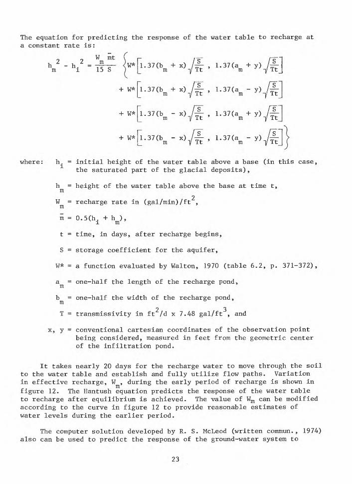
The equation for predicting the response of the water table to recharge at a constant rate is:

,2 . 2 m y T T* h — h = ———— \ W*11. i r- <-* XVVm i 15 S

w*[i.37<bm -x) V-, i.

+ W* 1.37(b - x) /-— , 1.37(a_ - y)

where: h. = initial height of the water table above a base (in this case, the saturated part of the glacial deposits),

h = height of the water table above the base at time t, m

2 W = recharge rate in (gal/min)/ft ,m

in = 0.5(h. + h ),i m

t = time, in days, after recharge begins,

S = storage coefficient for the aquifer,

W* = a function evaluated by Walton, 1970 (table 6.2, p. 371-372),

a = one-half the length of the recharge pond,

b = one-half the width of the recharge pond, m

2 3 T = transmissivity in ft /d x 7.48 gal/ft , and

x, y = conventional cartesian coordinates of the observation point being considered, measured in feet from the geometric center of the infiltration pond.

It takes nearly 20 days for the recharge water to move through the soil to the water table and establish and fully utilize flow paths. Variation in effective recharge, W , during the early period of recharge is shown in figure 12. The Hantush equation predicts the response of the water table to recharge after equilibrium is achieved. The value of Wm can be modified according to the curve in figure 12 to provide reasonable estimates of water levels during the earlier period.

The computer solution developed by R. S. McLeod (written commun., 1974) also can be used to predict the response of the ground-water system to

23

100< UJ

< <UJH Z< O

80

z <S 3 60< CL

F <

LLJ < > H

40

20

2 4 6 8 10 12

TIME, IN DAYS SINCE RECHARGE BEGAN

14 16

Figure 12. Variation of effective infiltration rate with time.

pumpage and recharge. The computer model predicted the response of the system to pumping 5,000 gal/min (300 1/s) from 5 wells (fig. 9) and recharging 4,000 gal/min (250 1/s) in a central recharge area (fig. 13).

RECYCLING

Recycling (reusing) some of the hatchery effluent reduces the amount of effluent released from the hatchery area, thereby reducing the potential for degradation of the regional ground-water system. Recycling also reduces the net withdrawal of ground water. The location of the recharge area relative to the cone of depression of the pumping well determines the amount of water recycled (reused), the amount that is released to the regional ground-water system, and the reduction of water-level declines.

A water-supply development and recharge system can be operated as an open, semiopen, or closed system. In the open system, water recharged downgradient and outside the cone of depression does not return to the supply well (fig. 14). The system also can be designed so that some (fig. or all (fig. 16) of the water returns to the supply well (recycling). In the open system no water-level declines and no reduction of natural ground- water discharge occurs downgradient from the recharge area. (For example, the flow at Mecan Springs would not be reduced.) However, the regional ground-water system bears the full impact of any degradation of water quality that might be caused by the recharged water. Recycling some or all of the recharge water reduces this effect on the regional ground-water system. Evaporation losses will occur while the water is exposed at the surface, but in most practical situations these losses will be negligible

15)

24

-5N |CP

is

tOOO 2OOO FEET

BOO METRES

EXPLANATION

--5 ——— Line of equal water-level change,

after one year of continuous pumping-rechargmg

Interval 5 feet (1.5 metres)

Well location

Each well pumping 1 000 gal/min

(63 l/s)

Recharge area

Recharging 4000 gal/min (252 l/s)

Figure 13. Computed water-level changes accompanying 5 000 gallons per minute (315 litres per second) pumpage and 4 000 gallons per minute(252 litres per second) recharge. Does not include effect of natural recharge.

25

Recharge outside the cone of depression

y y y y

Figure 14. An open system of water-supply development and recharge.

Recharge partlywithin the coneof depression

|l| y y y

/ \<

Water level rises in response to recharge

Figure 15. A semiopen system of water-supply development and recycling.

26

Recharge within the cone of depression

I Water level rises in response to recharge

Figure 16. A closed system of water-supply development and recycling.

(from near zero to a maximum of 4 gal/min (0.3 1/s) per acre (0.4 hm ) of open water at the refuge).

The water-supply development and recycling system studied at the Greenwood Wildlife Refuge recycled as much of the waste water as possible. The supply well was located in the center of the infiltration pond so that all recharge was within the cone of depression. Increased concentrations of objectionable materials would occur most rapidly in this system, and degradation of the regional ground-water system would be minimized.

For 15 months water pumped from well Ws-642 recharged the ground-water system through an infiltration pond created in a shallow natural depression enclosed by dirt walls approximately 200 ft (60 m) on a side (fig. 17). A pond was chosen because waste water from the fish-rearing facility could be supplied to the pond by gravity flow, and the pond confined the recharge water, providing maximum recharge within the cone of depression. The soil and grasses in the pond were not disturbed. Pumpage was held approximately constant at 300 gal/min (20 1/s). Water-level changes in response to pumping and recharging were monitored throughout the period.

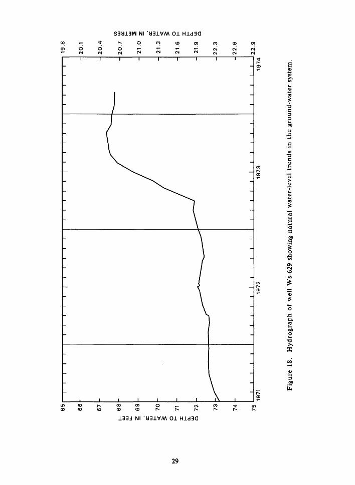
The effect of natural recharge had to be separated from the effect of recharging. Wells at the north side of the refuge, such as Ws-629, are more than 1,500 ft (460 m) from the recycling test site, and are little affected by pumping well Ws-642. Water-level changes in these wells were

27

Ws-637 1%-inch diameter

Ws-633

Ws-634

^ Ws-642 Ws-635 Pumping well

diameter

Ws-636-Infiltration pond 206 feet square

Wfe-645

Ws-644

0 50 100 FEETI ' ' V ' 'I- • • ,'0 10 20 30 METRES

EXPLANATION

"0. Observation well All observation wells are 2-inch diameter except as specifically noted

Ws-633 Sequential county well number

Figure 17. Detailed map of the recycling area.

1

28

DEPTH TO WATER, IN FEET

^J ^J vj O) o> N>_____-*_____O_____CO 00

1 1 I T

d >-i<D

CO

ffi

Oera >-i P•osro*••>

ON to

COsr o

era3 Pr»d

Ol 3 D.

3 <-*tr

era >iOd3D.

J

10 to M N) N)N) _,_»_,_» p O

CO CO O) CO O

DEPTH TO WATER, IN METRES

assumed to represent natural water-level trends in the regional ground-water system (fig. 18). Subtracting natural water-level trends from water-level fluctuations observed at the recharge site defined the net effect of recycling.

Recycling significantly reduced water-level declines normally resulting from pumping. Figure 19 shows drawdowns for a pumping rate of 300 gal/min (20 1/s) compared to observed drawdowns. By the end of the study the actual drawdown was only about 0.5 ft (0.2 m) in well Ws-643, 210 ft (64 m) from the pumping well, but would have been nearly 3 ft (0.9 m) without recycling.

The long-term response of the aquifer to combined pumping and recycling can be predicted with reasonable accuracy using the effective pumping rate. Using figures 7 and 8 with an effective pumping rate of 50 gal/min (3.2 1/s) provided a reasonable reproduction of observed drawdown (fig. 19). The effective pumping rate defines the recycling efficiency of the recycling system (E = {actual pumping rate - effective pumping rate) v actual pumping rate). Using the effective pumping rate (or Q {l-E}) with techniques for predicting drawdown (figs. 7 and 8) greatly simplifies the procedure for predicting aquifer response to combined pumping and recycling (but does not account for the effect of natural recharge (fig. 18)).

tu 1LU I

oQ

2 2Q

I I T

Predicted (Q=50 gal/min 3.1I/S )

Observed water-level change minus

the effect of natural recharge

December 1972 through February Well Ws-643 is 210 feet(64 m) from the pumping well,Ws-642 __________I___________I___________I___________I

0.3

0.6

100 200 300 400

TIME, IN DAYS SINCE PUMPING BEGAN

0.9500

Figure 19. Water-level changes in well Ws-643 during recycling.

30

Recycling efficiency for the system used during this study was 83 percent. The actual pumping rate was 300 gal/min (20 1/s); but the effective pumping rate was 50 gal/min (3.2 1/s). This efficiency reflects water evaporated at the infiltration pond surface or recharged outside the cone of depression. Evaporation from the pond and raceway surfaces did not exceed 4 gal/min (0.2 1/s) (assuming a maximum evaporation rate of 6 in (15 cm) during July (Devaul and Green, 1971, pi. 1) and a total open-water surface of 1 acre (0.4 hm^)). However, test drilling encountered some thin clay layers, and, although the clay layers are not areally extensive, some of the recharge water may be diverted laterally to eventually reach the water table outside the cone of depression. The cone of depression on a sloping water table may be asymmetric and further contribute to the amount of recharge water not captured within the cone. Recycling systems approaching 100 percent efficiency (fig. 16) may result where hydraulic and geologic conditions permit.

As the effective pumping rate decreases (recycling efficiency approaches 100 percent) predicted drawdown near the pumping wells may be in error. As the effective pumping rate approaches zero, the predicted drawdowns also approach zero. However, a gradient toward the well must exist to maintain flow toward the well—even though it may extend only a short distance from the pumping wells. Analysis of the three-dimensional flow system would provide a rigorous definition of drawdowns, but is beyond the scope of this report. The approximate technique presented provides reasonable estimates of drawdown in most practical applications.

The recycling efficiency may reflect both the hydraulic efficiency (relative location of withdrawal and the recharge sites (figs. 14, 15, 16)) and the schedule of withdrawal and recharge. (Schedule refers to the period during which water is recharged within the cone of depression relative to the total withdrawal period.) For example, water-level declines in a system with 100 percent hydraulic recycling efficiency recharging only 6 months each year would be equivalent to those in a system with 50 percent hydraulic efficiency recharging continuously.

The concept of overall recycling efficiency may be applied to other areas. The hydraulic efficiency is estimated by evaluating the physical characteristics of that site (soils and aquifer parameters). The estimated hydraulic efficiency combined with anticipated recharge schedules provides the overall recycling efficiency. Depending upon the recharge schedule, the overall efficiency may range from zero to the full hydraulic efficiency of the system. Time-drawdown curves, with the effective pumping rate, may be used to predict the long-term response of the local aquifer system to water-supply development. The concept of recycling efficiency is important when determining water quality and temperature-control capability of recycling, as discussed in the following sections.

TRACER STUDY

A tracer study was conducted to develop a technique for predicting response of the recycling system to hatchery-waste loading. Sodium chloride

31

(NaCl) was chosen as the tracer because it is not adsorbed in the soil nor taken up in th6 fish, and, in the concentration used, would cause no harmful effects in the ground-water system. Sodium chloride was introduced into the raceway effluent at a constant rate from September 6 through October 9, 1973. Fifty pounds (23 kg) of sodium chloride were added at a uniform rate each 24 hours, or an equivalent of 30.35 Ibs (13.8 kg) of chloride. Chloride concentration in the water supply increased to 14 mg/1 (milligrams per litre) (fig. 20) or about 12.4 mg/1 above the average level of 1.6 mg/1 observed immediately before the tracer was added. (Although chloride levels vary naturally, concentrations were stable before the tracer was added, and natural variations during the tracer study were minor relative to changes caused by the addition of the tracer.) Monitoring of the water supply continued until chloride concentration decreased nearly to previous levels (about 5 months).

A mathematical relation was used to analyze the observed changes in chloride concentration. The following equation accounts for concentration changes in response to recycling within the local ground-water system and exchange with the regional system.

c(t) = QC(t-l) + qEC(I) - qC(t-l) + q'CQ)) (1)

where: C(t) = concentration in the recycling system (measured in the well water) at time "t",

C(t-l) = concentration in the recycling system (measured in the well water) during the preceding time step, "t-1",

C(I) = concentration in the recharge water = (C(added)} + (C(t-l)},

C(o) = initial background concentration in the regional ground- water system,

Q = amount of water included in the recycling system at any given time,

q = amount of water pumped during the period from (t-1) to (t),

q f = inflow (make-up) water entering the recycling system from the regional ground-water system; balanced by an equal amount of water lost to the regional ground-water system (q f = q{l-E», and

E = efficiency of the recycling scheme being used (water actually reused -r water pumped) .

Terms in the equation are known or are estimated from water-level data. The terms C(I), C(o), and q are known (or specified), and q f is defined

32

CHLORIDE CONCENTRATION, IN MILLIGRAMS PER LITRE-» _» 10

Ol O 01 O

c n>N>O

O cr

OQn>

5 § W H

CLn>

O^

B"

&•n>

OQ "-»n> o «< o5'

OQ

>j m£> CD

when E and q are known. E was estimated in the preceding section (E = 0.83). Q is obtained from water-level analysis, as described below.

Q is the water taken into the active recycling system from storage in the ground-water system. While water is being taken from storage, water levels decline rapidly. When recycling begins, the rate of decline slows and subsequently water levels rise. When enough water has been taken from storage to sustain the recycling system, water levels stabilize. Figure 19 shows the initial fluctuation of water levels and the return to stable conditions after 30 days. Assuming a linear transition from the first instant of pumping, when all water comes from storage, to equilibrium, when all water is being recycled, Q equals one-half the time to equilibrium multiplied by the average pumping rate during the period. (Recycling efficiency need not be considered when estimating Q, because the inflow and outflow of makeup water balance, and net withdrawal from storage does not change.) In the current analysis:

Q = 15 (one-half of the 30 days to equilibrium (fig. 19)) x 0.43 x 10 6 gal/d (1.6 x 1Q6 1/d)

= 6.45 x 106 gal (24.4 x 106 1)

= 53.8 x 106 Ibs (24.4 x 10 6 kg).

Equation (1) is used when the recharge water is modified externally (in the raceways, infiltration pond, or soil column above the water table). When no change is imposed externally, the term "q f C(t-l) n replaces the terms "qEC(I) - qC(t-l)", and equation (1) is:

c(t) = QC(t-l) + q'C(o) - q'C(t-l) ^ (2)

which is further simplified to the form:

c(t) = EQC(t-l) + q'C(o) (3)

Equation (1) is used when sodium chloride is being added and equation (3) is used when the chloride concentration is being dissipated by dilution in the regional ground-water system (fig. 20). The values for the constant terms of the equations are as tabulated below.

C(o) =1.6 mg/1 (Cl),

Q = 53.8 x 106 Ibs (6.45 x 10 6 gal) = 24.4 x 10 6 kg (from water-level analysis),

q = 3.6 x 106 Ibs/d (300 gal/min = 0.43 x 106 gal/d) = 1.6 x 10^ kg/d, times the number of days in the time step,

34

q' = 0.6 x 106 Ibs/d (50 gal/min) = 0.07 x 106 gal/d) = 0.3 x 10" kg/d, times the number of days in the time step, and

E = 0.83 (from water-level analysis).

The calculated chloride concentrations agree well with observed values (fig. 20) except during the early part of the tracer study, and just after the application of sodium chloride has ceased. The difference during the transition periods is the result of different travel times for particles within the recycling system. Particles recharged near the well arrive more quickly than those recharged near the outer limit of the pond. Particles recharged near the outside of the pond continue to arrive for some time after application of the tracer stops. Diffusion, dispersion, and length of travel path affect the departure between the predicted and observed concentrations during the transition periods. The equations might be modified for these periods, but the.modifications are complex and beyond the scope of this study.

Equations (1) and (3) provide reasonable estimates of tracer-concentration changes in the recycling system. The predicted peak was within 2 mg/1 of the actual peak (fig. 20), and the peak probably would be most important to hatchery operation or ground-water protection. Also, had the tracer concentration been greater, or had the test run longer, the predicted peak may have been even closer (relatively) to the observed peak. The actual peak occurred approximately 8 days later than predicted because of the travel time described before. The error probably would not increase for longer test periods. The predicted dissipation of the tracer after the test period is reasonably close to observed data, particularly in terms of predicting the time required to return to background levels.

The tracer analysis confirms that recycling was achieved and provides a technique for predicting the level of contaminants in the water supply introduced during recycling. The equations are valid only for conservative constituents—conservative in that only mixing affects the constituent being considered. However, concentrations of those contaminants that are retained unchanged within the recycling system will increase most rapidly and probably will be the first to adversely affect the feasibility of recycling, and the equations are adequate with respect to these contaminants.

WATER-QUALITY ASPECTS

Recycling the water added oxygen, accomplished filtration, resulted in some nutrient uptake by the soil and vegetation, and reduced the effect of effluent disposal on the regional ground-water system. Oxygen was added by agitation during pumping and from the atmosphere in the open raceways and pond. Filtration occurred as the water moved through the grasses and soil at the bottom of the pond and through approximately 100 ft (30 m) of unsaturated sand before reaching the water table. Plants and algae in the infiltration pond utilized some nutrients. Because 83 percent of the

35

effluent was recycled, only 17 percent was released to the regional ground- water system.

The fish-rearing operation provided an effluent similar to that of a typical hatchery operation. Rainbow trout fingerlings were raised in raceways for 12 of the 15 months of recycling. The fish gained 6,100 Ibs (2,800 kg) on 8,650 Ibs (3,900 kg) of food pellets. Water quality was monitored in the water supply, as well as in the local ground-water system, to observe changes resulting from recharging and recycling the waste water from the fish-rearing operation.

Nutrient concentrations in the water supply changed most during recycling. Other constituents are either not produced in significant quantities during fish-rearing operations, or are effectively removed in a simple filtration system. (Recycled water moved through 100 ft (30 m) of unsaturated sand before reaching the water table, and removal by filtration and adsorption is assumed to be complete.) Except for the nutrients chemical composition of the water supply did not change significantly during recycling (table 2). Nitrate-nitrogen concentrations ranged from 1.6 to 3.6 mg/1 during the study, fluctuating with loadings imposed by the fish-rearing facility. Of the nutrients, phosphates are effectively removed by adsorption, replacement, or precipitation in natural soils (Dudley and Stephenson, 1973, p. 11-12), so observed variations in phosphate concentrations were assumed to be natural, or the result of inconsistent analytical techniques.

Nutrients produced in the rearing facility would be primarily the nitrogen forms, principally as the ammonium ion. No oxygen deficiencies were noted in the recycling system during the operation, so oxidation of ammonium-nitrogen (NH^-N) to nitrate-nitrogen (N03~N) within the system was complete. (Any organic nitrogen produced probably also was broken down and oxidized to N03-N.) Dissolved-oxygen (DO) levels in the water supply ranged from 9 to 11 mg/1. In the raceway effluent, DO did not drop below 5 mg/1, and in the infiltration pond, DO ranged from 5 to 15 mg/1. Although ammonium-nitrogen of nearly 1 mg/1 occurred in the effluent, where oxidation was occurring but not completed (table 2A), it was typically less in the infiltration pond (table 2B), and ammonium- nitrogen levels in the water supply were negligible (table 2).

The nitrogen added to the system during the study was estimated from weight of food and weight gained by the fish. These estimates were provided by Paul Degurse (oral commun., 1974), biologist, Wisconsin Department of Natural Resources. The average nitrogen (N) content of the fish food was 6.4 percent, and the nitrogen (N) content of the fish flesh is estimated to be 3.2 percent. Hence, 6.4 percent of the food minus 3.2 percent of the fish weight gained is the estimated total nitrogen load during the period of operation.

Approximately 350 Ibs (160 kg) of nitrogen was added to the recycling system during the rearing operation. A total of 8,550 Ibs (3,900 kg) of food were used (547 Ibs (248 kg) of nitrogen) and 6,100 Ibs (2,800 kg) of fish were raised (195 Ibs (88 kg) of nitrogen). The difference between

36

the amount of nitrogen added and the amount harvested (547 - 195 = 352 Ibs {160 kg}) is the amount added to the recycling system. Table 3 presents the monthly nitrogen loading for the period of operation. Because there was an adequate supply of oxygen in all recycled water, nitrogen was expected to appear in the oxidized state as nitrate-nitrogen (N03~N) (table 2).

The nitrate-nitrogen levels expected during the period of operation are calculated using the nitrate-nitrogen input (table 3) with equation (1), assuming that the nitrate-nitrogen behaves as a conservative element. Nitrate-nitrogen levels in the water supply did not exceed 4 mg/1. Observed nitrate-nitrogen concentrations are compared to the predicted concentrations in figure 21. The predicted concentrations are near observed values through September 1973, and follow the trends. However, the observed levels after October 1973, when the nitrogen loading was reduced, are lower than predicted levels. Predicted levels decrease somewhat, however, so part of the difference is due to the transition effect noted during the tracer study. Part of the difference also may be the result of nitrogen removal by plants and algae in the infiltration pond. (Bacterial denitri- fication (an irreversible loss of nitrogen as N2 gas) occurs in anaerobic conditions—because oxygen was available throughout the recycling system, denitrification was not likely.) There are not sufficient data available from this study to consider this nitrogen sink in equation (1), so predicted levels will be higher (more severe) than those that would actually occur. (The nitrogen is only temporarily tied up in the vegetation, and the plants would have to be harvested periodically to remove the nitrogen from the system.)

The equations developed may be used to predict the response of the local aquifer system to the nitrate-nitrogen loading of a full-scale hatchery operation. The equations also apply to other conservative constituents dissolved in the recycled water.

The chemical quality of the recycling water can be monitored in order to detect changes and to modify operations to prevent severely degrading the quality of the regional ground-water system. As long as the volume of water within the recycling system (Q in equations (1) through (3)) is less than the volume of water outside of the recycling system, recycling will cause greater quality changes in the water supply than in the regional system. The loading retained in the recycling system is greater than that released to the regional system if the recycling efficiency is 50 percent or greater. At most sites the active recycling system will be only a small part of the regional ground-water system. Then, quality changes will be greater within the recycling system and problems can be detected and corrected before the regional system experiences an equivalent change. This approach probably is more restrictive than necessary and provides a means to assure protection of the regional ground-water system.

If recycling efficiency is less than 50 percent, contamination of the regional ground-water system must be considered. Evaluating the impact of contamination requires determining the natural flow through the area of

37

Table 2.—Analysis of water

(All values are in milligrams per litre except specific

Sample date

Silica (Si02 )

Iron (Fe)

Manganese (Mn)

Calcium (Ca)

Magnesium (Mg)

Sodium (Na)

Potassium (K)

Bicarbonate (HC03 )

Sulfate (804)

Chloride (Cl)

Fluoride (F)

Nitrate-nitrogen (N03-N)

Ammonium-nitrogen (NH4-N)

Phosphate (PO^)

Dissolved solids

Hardness as CaC03

Conductance (micromhos)

PH

Color

8-8-72 l 18 o 3 DNR2

0.100

.036

40

20

2.4

.6

208

11

8.0

.1

1.2 2.52

.08

199

180

334

7.9

5

2-1-73 3-1-73 3-29-73 DNR2 DNR2 DNR2

0

.019

22.5

1.62

1.20

.75

1.08

2.56 2.72 2.27

.05

.14 .08 .03

3-29-73

10

.030

0

45

20

1.2

.6

222

7.8

2.0

.1

2.6

207

200

360

7.8

10

6-5-73 DNR2

0

22.5

1.66

1.05

.55

.90

2.36

.06

.04

1Analyses by U.S. Geological Survey lab except as noted.

2Analyses provided by Wisconsin Department of Natural Resources.

3Values increased by addition of tracer (NaCl) during tracer study.

38

from supply well Ws-642 1

conductance, pH, and color, which are in standard units)

6-27-73 7-27-73 8-26-73 DNR2 ^'-'J DNR2 DNR2

9.4

0.062 .040

0

23 43

1.66 23

1.25 1.3

.60 .6

222

6.2

1.14 5.3 0.68 1.77

.1

2.63 1.6 2.85 3.52

.03 <.01 <.01

.05 .26

205

200

361

7.5

5

9-2-73 DNR2

10

.060

.042

52

223 2.8

.8

254

8.2

1.53 3 7.5

.1

3.64 1.2

.133 234

220

3 405

7.4

3

10-31-73 11-29-73 ? , DNR2 DNR2 :

9.0

.050

0

42

283 6.0

1.2

251

7.0

3 9.82 3 7.79 3 5.5

.2

1.89 2.26 2.3

<.01

.05 .04 .033 233

2203 418

7.8

5

39

Table 2A.—Analyses of

(All values are in milligrams per litre except specific

Sample date

Silica (Si02 )

Iron (Fe)

Manganese (Mn)

Calcium (Ca)

Magnesium (Mg)

Sodium (Na)

Potassium (K)

Bicarbonate (HC03 )

Sulfate (804)

Chloride (Cl)

Fluoride (F)

Nitrate-nitrogen (N03-N)

Ammon i um-n i t r og en (NH4-N)

Phosphate (P04>

Dissolved solids

Hardness as CaCC>3

Conductance (micromhos)

pH

Color

2-1-73 3-1-73 3-29-73 DNR2 DNR2 DNR2

0

22.7

1.62

1.20

.75

1.11

2.62 2.37 2.19

.68

.16 .18 .20

3-29-73

8.3

.08

.04

42

22

1.0

.7

218

7.0

2.2

.1

2.4

208

200

361

7.6

5

6-27-73 07 DNR2 6-27'73

12

0.06 .03

.01

23 43

1.66 23

1.45 1.6

.68 .7

222

7.4

.705 6.2

.1

2.66 1.7

.72

.22

226

200

369

7.6

0

1 Analyses by U.S. Geological Survey lab except as noted.

2 Analyses provided by Wisconsin Department of Natural Resources.

3Values increased by addition of tracer (NaCl) during tracer study

40

the raceway effluent 1

conductance, pH, and color, which are in standard units)

7-27-73 8-26-73 9-2-73 10-31-73 DNR2 DNR2 DNR2 DNR2

15

.07

.05

67

143 5.4

1.2

248

9.0

0.76 1.64 1.34 3 12 3 9.61

.1

3.63 3.26 3.69 2.5 2.04

.04 .16 .20 .29

.34 .26 .12

252

2203 414

8.2

5

11-29-73 12-21-73 DNR2 DNR2

8.9

0

42

29

3.9

252

7.4

3 7.52 3 6.8

.1

1.62 2.5

.27

.55 .033 254

2203 426

7.6

0

41

Table 2B.—Analyses of water

(All values are in milligrams per litre except specific

Sample date

Silica (Si02 )

Iron (Fe)

Manganese (Mn)

Calcium (Ca)

Magnesium (Mg)

Sodium (Na)

Potassium (K)

Bicarbonate (HC03 )

Sulfate (804)

Chloride (Cl)

Fluoride (F)

Nitrate-Nitrogen (N03-N)

Ammonium-Nitrogen (NH4-N)

Phosphate (PC^)

Dissolved solids

Hardness as CaC03

Conductance (micromhos)

pH

Color

1-18-73 2-1-73 3-1-73 3-29-73 DNR2 DNR2 DNR2 DNR2

0.06

22.7

1.60

1.35

.90

.95

2.49 2.56 2.36 3.15

.03

.06 .11 .12 .27

3-29-73

7.3

.02

.02

42

22

1.1

.7

218

7.0

2.1

.1

2.3

206

200

356

7.8

0

6-27-73 DNR2

0.06

22.7

1.66

1.30

.92

.81

2.99

.56

.11

6-27-73

8.9

.02

.01

43

22

1.6

.7

214

11

6.0

.1

1.6

216

200

361

7.4

5

1 Analyses by U.S. Geological Survey lab except as noted.

9Analyses provided by Wisconsin Department of Natural Resources.

q

Values increased by addition of tracer (NaCl) during tracer study.

42

from the infiltration pond

conductance, pH, and color, which are in standard units)

7-27-73 8-26-73 9-2-73 10-31-73 11-8-73 DNR2 DNR2 DNR2 DNR2 DNR2

10

.07

.02

65

143 6.2

1.0

252

8.8

0.54 1.68 1.31 3 12 3 9.92 3 8.83

.3

3.02 3.48 3.31 1.1 1.78 2.09

11-29-73 DNR2

16

.

.

45

213 2.

.

222

5.o o3 7.25 3 1.

.

2.63 1.

,73

09

01

1

8

6

4

1

9

.04 .34 .38 .18 .15 .21

41 .37 .20 .19 .25

3 244 3 210

220 200

3 418 3 360

7.2 7.8

4 5

43

Table 3.—Estimated NOyN loading produced by fish-rearing operations atthe Greenwood Wildlife Refuge and the resultant concentration increase

in the raceway effluent from January 18, 1973, to January 22, 1974

(Data provided by personnel of the Wisconsin Department of Natural Resources)

Date Days in period

N03~N loading (Ibs)

Calculated increase in NO«-Nconcentration in racewayeffluent during period 1

(mg/1)

1973

January February March April

1328313

1330353

(No fish in raceways from 4-4-73 to 6-5-73)June 30 24July 31 36August 31 45September 30 55October 31 44November 30 21December 31 25

1974

January 21 20

0.28 .30 .31 .03

.27

.32

.40

.55

.39

.21

.22

.25

on a constant flow rate of 300 gal/min (18.9 1/s) (3.6 x 106 lbs/d or 1.6 x 106 kg/d).

consideration. The natural flow beneath the Greenwood Wildlife Refuge, defined by Darcy's Law, is the product of the hydraulic conductivity, the gradient, and the cross section through which the flow passes. The average hydraulic conductivity at the refuge is 160 f t/d (50 m/d) , the gradient is approximately 20 ft/mi (3.78 m/km) , and the area, based on an average width of 1.5 mi (2.4 km) and an average saturated thickness of 100 ft (30 m) is 800,000 ft 2 (74,000 m2 ) . Then the natural flow (Q) is 1.3 x 109 gal (4.9 x 109 1) per year, or 1.1 x IQlO ibs (4.9 x 109 kg).

With the natural flow through the area, recharging 11,000 Ibs (5,000 kg) of a substance, assuming complete and uniform mixing, increases the con­ centration in the regional ground-water system 1 mg/1. (Mixing is incomplete near the disposal site but is assumed complete short distances downgradient and the equations predict concentration changes in the regional ground- water system adequately.) In the current study, producing 1 Ib (0.45 kg) of fish released 0.06 Ib (0.03 kg) of nitrate-nitrogen. If this figure

44

10

cc.

ff

7

cc (D

6 5z O I- 2

4

ro

O

2

i i

i i—

—r

o-^

o

X

1 I

Calc

ula

ted c

oncentr

ation

-—_

R

ecy

clin

g e

ffic

iency=

100 perc

ent

i r

XX

X

*

f

f

f

fXX

• Ca

lcu

late

d co

nce

ntr

atio

n

Recyclin

g e

ffic

ien

cy =

83

p

erc

en

t

X0bse

rved d

ata

J_____I

I_____I

J_____I

J_

__

__

IJ_____I

MM

J J

19

73

0

NF

M

1974

Fig

ure

21.

N

itra

te-n

itro

gen

conce

ntr

atio

n c

han

ges

in

the

wat

er s

uppl

y du

ring

rec

ycli

ng.

remains valid for larger production capacities, production of 200,000 Ibs (100,000 kg) of fish would release 11,000 Ibs (5,000 kg) of nitrate-nitrogen. No hatchery in Wisconsin approaches this production level, so full-scale hatchery production would have little effect on nitrate-nitrogen concen­ trations in the regional ground-water system even if none of the water were recycled. With recycling, the effect on the regional system would be further reduced.

WATER-TEMPERATURE REGIMEN

Temperatures of the water supply during continuous pumping and recycling (June 1973 to March 1974) ranged between 7.0°C (45°F) and 14.0°C (57°F), with a mean of 10.7°C (51°F). Mean daily air temperatures during the same period ranged from -25°C (-13°F) to 27°C (81°F), and water temperatures in the infiltration pond were intermediate between the air and ground- water temperatures (fig. 22).

A mathematical relation describes the observed fluctuations and predicts pond temperatures and ground-water temperatures based on the initial (background) ground-water temperature and the air temperature. The relation is an energy-balance equation relating the mass and temperature of water recharged in a given period to the mass and temperature of water in the ground-water system affected by the recharge water. The water recharged in a given period is simply the pumping rate multiplied by the recycling efficiency (83 percent). The water in the ground-water system affected by recharge (Q, as described earlier) is 53.8 x 106 Ibs (6.45 x 106 gal) (24.4 x 1Q6 kg). The following equation predicts the average pond temper­ ature at the end of a given pumping period (I):

PT(I) = K{AT(I) - GWT(I-l)} + GWT(I-l) (4)

I = computation period (in this study 1=1 month),

PT(I) = pond temperature at the end of the computation period,

AT(I) = mean air temperature during period,

GWT(I-l) = ground-water temperature (water-supply temperature) at the beginning of the computation period, and

K = response coefficient, based on observed data, which defines the response of the pond temperature to the influence of the water-supply temperature (ground- water temperature) and the air temperature.

The ground-water temperature is then given by the following equation:

GWT(I) = {Q x GWT(I-l)} + {q x PT(I)> (5)

46

I I I I I I

Air temperature

Ground-water (water supply) temperature

Pond temperature

Calculated ground-water temperature (GWT)

Calculated pond temperature (PT)

-25 -13JUNE JULY AUG SEPT OCT NOV DEC JAN FEB MAR

1973 1974

Figure 22. Air temperatures and observed and calculated water temperatures during recycling.

47

GWT(I) = ground-water temperature at the end of the computation period,

Q = volume of water in the local ground-water system affected by recharge, and

q = recharge during the computation period, equal to pumpage times the recycling efficiency.

The calculations are then repeated in sequence to define the pond temperature (PT from equation (4)) and the ground-water temperature (water-supply temperature = GWT from equation (5)) for the end of each computation period (I).

The effect of makeup water (17 percent of the pumpage) at the initial ground-water temperature should be included, as in equations (1) and (3) developed earlier. However, there is no way to determine "background" (initial, or pretest) temperature after recycling is initiated, because the 17 percent of the recharge water released to the regional ground-water system does transmit some effect back to the part of the aquifer from which the makeup water subsequently will be supplied to the recycling system. Temperature is not conservative as are nitrate and chloride ions. Although the exchange of heat between the recharge water and the glacial deposits can be quantified (Stallman, 1963), it is beyond the scope of the current study. Rather than trying to modify the makeup-water temperature, this effect is included in the value of the response coefficient (K).

The response coefficient (K) was defined by applying equations (3) and (4) to observed data. Ten months of data were analyzed using 1-month intervals. (A shorter computation interval might reproduce more faithfully the pond-temperature fluctuations, but the number of calculations involved may necessitate use of a computer.) Two K values were actually determined, the one for the warm period (K = 0.30, April through October) is larger than that for the cold period (K = 0.13, November through March). Ice covered about 50 percent of the pond during the winter, which suggests that the value of K is directly related to the surface area of the pond exposed to the atmosphere. An example of the use of equations (3) and (4) to reproduce the temperature regimen observed during the study period is presented in table 4.

The K values are unique to the infiltration pond/recycling pattern used during this test. Although it may be desirable to define the coefficient (K) for different infiltration pond/recycling patterns on the basis of observed data, the current values are adequate for predictive purposes as discussed later. The K values defined are independent of the system of units used and can be used with either English or SI units without modification.

48

RECYCLING AS A RESOURCE-MANAGEMENT TOOL

The techniques developed in this study can be used to predict the response of an unconsolidated aquifer system to recycling water from a full-scale-hatchery operation. Equation (1) predicts the concentration of N03~N (or other conservative ions) based on the loading produced by the hatchery and the efficiency of the recycling system. Equations (4) and (5) predict the water-supply temperature based on the recycling efficiency of the system and the recycling schedule. The overall recycling efficiency of the system (hydraulic efficiency combined with recharge schedule) used with drawdown curves (figs. 7 and 8) predicts the aquifer response to water-supply development.

The response of the aquifer system at the Greenwood Wildlife Refuge to development of a hypothetical hatchery can be predicted as follows. Assume that production of the hypothetical hatchery is 100,000 Ibs (50,000 kg) of salmonids annually. Hatchery facilities capable of this production level are considered optimum in the Wisconsin fish-production program (J. H. Klingbiel, oral commun. s 1974). The hatchery would require a water supply of approximately 3,000 gal/min (189 1/s), would use 240,000 Ibs (110,000 kg) of food annually, and produce a loading of 10,800 Ibs (5,000 kg) of N03~N. The water-supply requirement could be developed from the aquifer at the refuge without recycling, so the effect of water-supply development will be considered last. However, changes in water quality and temperature in response to recycling the hatchery effluent in the ground-water system may be significant and will be considered first.

NITRATE-NITROGEN CONCENTRATIONS

The response of the local aquifer system at the Greenwood Wildlife Refuge to the hypothetical effluent loading was predicted using equation (1). The hypothetical nitrate-nitrogen loading was based on data from the Wild Rose State Hatchery. The feeding schedule at the Wild Rose Hatchery from March 1973 through February 1974 provided the nitrate-nitrogen loading used for the hypothetical hatchery. An average conversion ratio of pounds of food to pounds of fish gained was reported to be 1.75, so that nitrate- nitrogen loading is {(1.75 x 0.064 - 1.00 x 0.032)/I.75} times the pounds of food fed each month (table 5). The recycling efficiency (E) is assumed to be 83 percent, as in the present study. The volume of the ground-water system affected (Q) is assumed to be 15 times the daily pumpage as in the current study. Figure 23 shows the annual variation in nitrate-nitrogen concentrations expected in the water supply in response to these hypothetical conditions after equilibrium is achieved. Equilibrium is achieved after approximately 20 months, and subsequent monthly values will repeat on an annual cycle as shown unless the nitrate-nitrogen loading is changed. The peak concentration (7 mg/1) is within drinking water standards (10 mg/1 as N03-N, McKee and Wolf, 1963, p. 224).

49

Table 4.—Water-temperature regimen reproduced using equations (4)

1973-1974 May June July

2 Pumpage rate (q) in millions of pounds per month 1 75.0 93.0

Amount of water in the recycling system (Q) plusthe amount pumped during the month being 128.8 146.8 considered (q) l

Mean air temperature (AT) in °C 18.3 20.8

Difference between air temperature and ground- 117 water temperature (AT-GWT), in °C

Product of response coefficient (K) and ~ ~ ~ r temperature difference (AT-GWT)

Pond temperature (PT) in °C, calculated from in _ 1? ,. • / * \ J. \J • .3 JL ^£ • Oequation (4)

Observed pond temperature at the end of each ins 1 9 si • s\ s-. JL v • _J JL ^ • _ymonth, in °C

Product of pumpage (q) and calculated pond 7R7 __ i 171 onf-r. —— \ / O / . DU J. , 1 / 1 • OU

temperature (PT)

Product of amount of water in the recycling system _ 8 _ _, .„„ ^o (Q) and the ground-water temperature (GWT)

Ground-water temperature (GWT) in °C, calculated 3 7 9 Q 1 11 3 from equation (5)

Observed water-supply temperature (assumedto be equal to the ground-water temperature), 7.0 9.0 11.5 in °C

K = 0.30 April through October.

K = 0.13 November through March; partial ice cover on pond.

Values of q and Q are in millions of pounds. However, the two values define a ratio in equation (5) so they could be in any consistent units and the results would be the same.

o

Pumping began on June 5; q is based on 25 days of pumpage in June.

o

Initial ground-water temperature (GWT) affected by earlier pumpage and recharge.

50

and (5) with K values determined from observed water temperatures

Aug. Sept. Oct. Nov. Dec. Jan. Feb. Mar.

93.0 90.0 93.0 90.0 93.0 93.0 84.0 93.0

146.8 143.8 146.8 143.8 146.8 146.8 137.8 146.8

20.9 15.1 11.8 1.4 -8.8 -8.9 -8.0 2.0

9.6 2.0 -1.7 -11.8 -21.1 -19.5 -17.0 -5.7

2.9 .6 -.5 -1.5 -2.7 -2.5 -2.2 -.7

14.2 13.7 13.0 11.7 9.6 8.1 6.8 7.0

14.5 14.0 12.0 10.0 8.0 8.0 7.0 ————

1,320.60 1,233.00 1,209.00 1,053.00 892.80 753.30 571.20 651.00

607.94 704.78 726.30 710.16 661.74 570.28 484.20 414.26

13.1 13.5 13.2 12.3 10.6 9.0 7.7 7.3

13.0 14.0 13.0 12.5 10.5 9.0 7.5 ————

51

Table 5.—Feeding schedule for the Wild Rose State Fish Hatchery and the equivalent NO-^-N loading on a hypothetical recycling system

(Data provided by Donald Czeskleba, fish hatchery manager)

Month

JanuaryFebruaryMarchAprilMayJuneJulyAugus tSeptemberOctoberNovemberDecember

Food (Ibs)

18,15016,00019,45022,00025,80022,80024,90027,90018,65013,45016,60014,500

Equivalent N03-N loading 1

(Ibs)

817720875990

1,1611,0261,1201,256

839605747652

Increased N03-N concentration in the

raceway effluent (mg/D

0.73.71.78.92

1.04.95

1.001. 12.78.54.69.58

Based on an average 1.75 conversion ratio; nitrogen content of food minus nitrogen content of fish produced, reported as nitrate nitrogen.

Based on a constant flow rate of 3,000 gal/min (189 1/s) = 36 x 106 Ibs/d (16.3 x 106 kg/d).

TEMPERATURE CHANGES

Average monthly water-supply temperature and pond temperatures also can be estimated. Equations (4) and (5) were used with the K values determined during this study and the 30-year "normal" monthly air temperatures reported by the U.S. Weather Bureau for the Hancock Experimental Farm (U.S. Department of Commerce, 1931-74). Predicted water-supply temperatures in response to continuous pumping and recharge during a normal year (fig. 24) range from 7.0°C (45°F) to 14.5°C (58°F) and average 10.5°C (51°F).

SELECTIVE RECYCLING

Equations (4) and (5) also can be used to evaluate the potential of selective recycling for achieving optimum temperatures in the water supply. For those months when pond temperatures are lower than ground-water temperature water is not recycled, but is recharged downgradient from the recycling site, and makeup water coming into the system (q) is assumed to be at the initial ground-water temperature (9.5°C or 49°F). The water is recycled during the remaining months. The resulting water-supply temperature

52

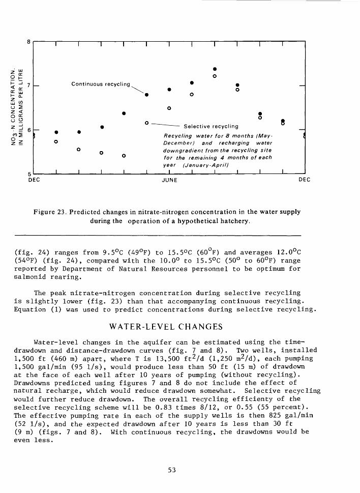
o ^z <O DCo ^

03 M

o

7

6

1 1 1 1 1 1

_ Continuous recycling^'X. •

•

0

Q

!~ • • r,

1

•

O

Selective

| Recycling waterO December) and

1 1 1 1

0

, _0

0 •recycling

for 8 months (May- {recharging water

O o downgradient from the recycling site° for the remaining 4 months of each

year1 1 1 1 1 15 ————————————————————————————————————

DEC JUNE

(January-April)\ 1 1 1 1

DE

Figure 23. Predicted changes in nitrate-nitrogen concentration in the water supply during the operation of a hypothetical hatchery.

(fig. 24) ranges from 9.5°C (49°F) to 15.5°C (60°F) and averages 12.0°C (54°F) (fig. 24), compared with the 10.0° to 15.5°C (50° to 60°F) range reported by Department of Natural Resources personnel to be optimum for salmonid rearing.

The peak nitrate-nitrogen concentration during selective recycling is slightly lower (fig. 23) than that accompanying continuous recycling. Equation (1) was used to predict concentrations during selective recycling.

WATER-LEVEL CHANGES

Water-level changes in the aquifer can be estimated using the time- drawdown and distance-drawdown curves (fig. 7 and 8). Two wells, installed 1,500 ft (460 m) apart, where T is 13,500 ft 2 /d (1,250 m2 /d), each pumping 1,500 gal/min (95 1/s), would produce less than 50 ft (15 m) of drawdown at the face of each well after 10 years of pumping (without recycling). Drawdowns predicted using figures 7 and 8 do not include the effect of natural recharge, which would reduce drawdown somewhat. Selective recycling would further reduce drawdown. The overall recycling efficienty of the selective recycling scheme will be 0.83 times 8/12, or 0.55 (55 percent). The effective pumping rate in each of the supply wells is then 825 gal/min (52 1/s), and the expected drawdown after 10 years is less than 30 ft (9 m) (figs. 7 and 8). With continuous recycling, the drawdowns would be even less.

53

ID

co 14_

CO

LU (J

COLU LLJCC.CD 12LU Q

Z

LUCCD 1-

DC 10 LUQ.

LU1-

ccLU1-

^

£ 8

R

1 1 1 1 1 1 1 1 1 1 1

O °

•• o

Selective recycling —————— ——— o0

Recyclingwater for 8 months (May-December)and recharging water downgradient from the °recycling site for the remaining 4 months of 9each year (January-Apr//)

— o —

3 C

• 4

O ° \

O ^o Continuous recycling

9— • —

.

1 1 1 1 1 1 1 1 1 1 1

61

-58HLUXZLU CCX

UL

COLU

-54 LU CCCDLUQ

Z—

LU CCD

-50 <CCLU Q.^r

LU1-

CL LU1-

<

-46 ^

4.3

DEC JUNE DEC

Figure 24. Average monthly water-supply temperatures expected in response

to a long-term recycling operation.

BENEFITS

Recycling water minimizes required effluent treatment, reduces water- level declines in response to water-supply development, and provides beneficial control of the water-supply temperature. Reducing or eliminating effluent-treatment requirements reduces the cost of construction and operation of treatment facilities. The cost of construction and operation of effluent-treatment facilities differs between sites, so benefits from recycling will be different at each site.

Reducing water-level declines reduces the cost of pumping. Power requirements are proportional to the pumping rate times the head loss— and the distance water is lifted from the water table to the surface may be a significant part of that head loss. At the refuge, where the lift

54

is approximately 100 ft (30 m), reducing drawdowns 1 ft (0.3 m) would reduce pumping costs 1 percent.

The cost of maintaining desirable water temperatures is reduced by recycling. Hearing costs are calculated on the basis of electric heating for direct comparison with pumping-cost calculations. (A more realistic evaluation at any location and at any time is obtained by multiplying by an appropriate ratio of costs of other fuels to the then-current electrical costs.) At the refuge the cost of heating 1,000 gal/min (60 1/s) 0.5°C (1°F) is $3.00 per hour, assuming a cost of $0.02 per kilowatt-hour for electric power. The theoretical pumping cost per 1,000 gal/min (60 1/s), with an average lift of 100 ft (30 m), is about $0.60 per hour. Continuous recycling produces a net gain of 1.0°C (2°F) and costs only 10 percent of the equivalent heating cost. Selective recycling produces a net gain of 3.0°C (5°F) and costs only 4 percent of the equivalent heating cost.

MULTIPURPOSE PONDSAn infiltration pond was used for recharging because, in addition

to the reasons stated earlier, ponds could benefit the management goals of the Greenwood Wildlife Refuge. The refuge provides forage and protection for the Greater Canada Goose, but the geese must leave the refuge to seek water. If permanent water bodies could be provided on the refuge as part of a hatchery development, the waterfowl-management potential of the refuge would be expanded significantly (Ralph Hopkins, oral commun., 1972).

The 300 gal/min (20 1/s) of water recharged during the study created and sustained a 1-acre (0.4-hm^) pond in a natural depression. Initial infiltration rates were 0.03 (gal/min)/ft^ (1.8 m/d) but diminished and stabilized at 0.01 (gal/min)/ft^ (0.6 m/d) after a few months of operation. This is apparently the result of concentrating fine materials and creating an organic mat at the pond bottom. The size of pond maintained by a given recharge rate could be estimated using figure 10 as a guide. The final size of the pond probably could be expected to stabilize at 3 to 4 times its initial size under normal operating procedures. Pond size need not increase if initial infiltration rates are maintained by physically removing the organic mat or preventing its formation by allowing the pond to be dry occasionally. Pond size also could be increased by artificially reducing the infiltration rate by mechanical compaction or the addition of a sealant, such as clay, to the pond bottom.

Enlarging ponds by reducing the natural infiltration rates may provide additional retention time and may affect the temperature response coefficient (K) used in equation (4). Then it would be desirable to redefine K on the basis of observed data. If retention time is increased, it is probable that K will increase during the summer, but, because of the ice insulation, the K value for the winter may change only slightly. If this is the case, the water-supply temperature could be maintained at a higher level during the winter or at the same level but with increased recycling.

55

The pond also may be of direct benefit to the hatchery operation. In the current study the pond size stabilized at approximately 40,000 ft 2 (3,700 m2 ), with an average depth of about 1.5 ft (0.5 m). This represents approximately 60,000 ft^ (1,700 m^) of water which might be used in certain phases of the fish-rearing operation.

The quality of the water in the infiltration pond appeared suitable for fish rearing throughout the study period. Ammonium-nitrogen levels in the raceway discharge (where oxidation was occurring, but not completed) occasionally exceeded 0.6 mg/1 (table 2A). However, ammonium-nitrogen levels in the pond never exceeded 0.6 mg/1 and usually were considerably less (table 2B). Although some nitrogen may have been released to the atmosphere, most was oxidized to N03~N in the pond. Mean temperatures in the pond ranged from 5°C (41°F) to 15°C (59°F), although instantaneous temperatures ranged from 0°C (32°F) to 21°C (70°F). Biochemical oxygen demand (BOD) in the pond did not exceed 4 mg/1. Although these character­ istics may not meet requirements for salmonid rearing, the infiltration pond would be suitable for more tolerant fish.

Little progression eutrophication occurred in the pond during the study. Examination of the insect fauna showed a relatively high diversity of families, genera, and species (R. A. Lidwin, oral commun., 1974), indicative of reasonably healthy conditions in the pond. Many varieties of typical pond fauna (notably Coleoptera, Hemiptera, and Diptera) were observed 4 months after the pond was formed. Increased biomass of Diptera and Ephemeroptera indicated some enrichment by the end of the study period; however, no indication of accelerated eutrophication (such as a predominance of more tolerant species) was noted. The study was too short to prove conclusively that healthy conditions in the pond would remain for long periods. However, the pond would probably be suitable for fish rearing for several years unless the rearing operation itself created unexpected stresses.

CONSIDERATION OF OTHER RECYCLING SCHEMESRecycling employing other recharge schemes may be feasible at the

refuge or at other locations. Recharge might be accomplished by ditches or trenches or by unconfined surface spreading. Spray irrigation is an effective means of effluent disposal. Although recycling might be accomplished by injection into the aquifer through recharge wells, this method would minimize many of the benefits achieved by recycling through surface spreading.

Ditches or channels can be designed long enough to infiltrate all the water before reaching the end of the channel, or they might be shorter— with a receiving pond at the end. In either case, deposition of fine material will eventually decrease infiltration rates, requiring cleaning and rehabilitation. Water-level changes and water-quality aspects of the two recharge schemes would be essentially identical.

56

Unconfined surface spreading may be an acceptable method for accomplishing recharge. The surface area would be larger than that of a pond for an equivalent rate of recharge. With the greater surface exposed to the air, the temperature changes would be greater (K would be larger—both summer and winter), and evaporation losses would be greater. Unconfined surface spreading probably is not a reasonable alternative for the Greenwood Wildlife Refuge, because it provides none of the waterfowl- management benefits of ponds.

Spray application may be reasonable at the refuge or at other sites. Crops raised at the refuge supplement the waterfowl-management program, and increasing crop production by irrigating may offset some of the cost of pumping and recharging. The nutrients in hatchery effluent may supplement fertilizer requirements and further offset operational costs. Because irrigation requirements are seasonal, it would be reasonable to combine spray irrigation with other forms of recharge. Practical irrigation rates are approximately equal to plant requirements, so that water used for irrigation would be consumed and there would be little or no recharge to the aquifer and no recycling. However, increasing crop production by irrigating and maintaining ponds during periods when they are most needed may make this scheme worthy of further consideration. Continuous spray application is not essential to crop production, results in operational difficulties during the winter, and provides few of the waterfowl-management benefits of ponds. Continuous spray application would not seem to be a practical alternative for the refuge site.

The ground-water supply available at the Greenwood Wildlife Refuge, Waushara County, Wis., is suitable for a cold-water-fish hatchery. The available water supply may be as great as 10,000 gal/min (600 1/s). The quality of the ground water meets reported criteria for hatchery supplies, and the temperature is acceptable for fish rearing (9.5°C {49°F}).

Recycling water within the local ground-water system can be an effective tool for management of available water resources for fish-hatchery develop­ ments. Recycling at the refuge provided a supply of 300 gal/min (20 1/s), with drawdowns equivalent to a pumping rate of only 50 gal/min (3 1/s). During the period of the recycling study no significant deterioration in chemical quality occurred in either the water supply or in the ground- water reservoir. Nitrate-nitrogen levels increased, but remained below 4 mg/1 throughout the study. Temperature of the water supply ranged from 7.0° to 14.0°C (45° to 57°F) during continuous recycling, but could be maintained between 9.5° and 15.5°C (49° to 60°F) by selective recycling.

The capability to operate a hatchery without effluent treatment and without environmental degradation will be important to future hatchery developments. The raceway effluent, after recycling within the ground- water system, was suitable for reuse in the raceway. Materials were

57

completely removed by filtration or adsorption or were maintained at satisfactory levels by exchange with the regional ground-water system. Because the system recycled more than 80 percent of the recharged water and released less than 20 percent to the regional ground-water system and because the regional ground-water system is much larger than the recycling system, water-quality changes in the water supply (within the active recycling system) were much greater than those occurring in the regional ground-water system. The effect on water quality of recharging hatchery effluent could be estimated based on the recycling efficiency of the pumping-recharging scheme. The effluent of a full-scale hatchery operation could be recycled in the ground-water system at the refuge, and the water supply would still meet State of Wisconsin and U.S. Public Health Service (1962) drinking water standards; the effect on the regional ground-water system would be minor.

The temperature-control aspects of recycling will be important to modern fish-hatchery developments. Maintaining water temperatures within the optimum range for fish rearing can significantly increase fish production obtained on a given amount of food. Selective recycling at the refuge could provide a net temperature gain of 3°C (5°F), and maintain the temperature of the water supply within the optimum range throughout the year. The cost of heating the water an equivalent amount might be 25 times greater than the cost of pumping and recycling (based on electric heating costs). In view of the potential energy shortage and rising fuel costs, recycling certainly would appear to warrant consideration in future hatchery-development programs.

58

SELECTED REFERENCES

Boulton, N. S., 1963, Analysis of data from nonequilibrium pumping tests allowing for delayed yield from storage: Inst. of Civil Engineers Proc. {London}, v. 26, no. 6693.

Bredehoeft, J. D., and Finder, G. F., 1973, Mass transport in flowingground water: Water Resources Research, vol. 9, no. 1, p. 194-210.

Devaul, R. W., and Green, J. H., 1971, Water resources of Wisconsin—Central Wisconsin River basin: U.S. Geol. Survey Hydrol. Inv. Atlas HA-367.

Dudley, J. G., and Stephenson, D. A., 1973, Nutrient enrichment of ground water from septic tank disposal systems: Upper Great Lakes Regional Comm., 131 p.

Holt, C. L. R., Jr., 1965, Geology and water resources of Portage County, Wisconsin: U.S. Geol. Survey Water-Supply Paper 1796, 77 p., 2 pis.

Konikow, L. F., and Bredehoeft, J. D., 1973a, Simulation of hydrologicand chemical-quality variations in an irrigated stream-aquifer system: Denver, Colo., Colorado Water Resources Circ. 17, 43 p.

______1973b, A water-quality model to evaluate water-management practicesin an irrigated stream-aquifer system: Paper presented at 15th Western Resources Conf., Boulder, Colo., 46 p.

Kramer, Chin, and Mayo Consulting Engineers, 1969, A comprehensive plan for Wisconsin's trout and salmon hatchery development program: Seattle, Wash., 231 p., 99 figs.

McKee, E. J., and Wolf, H. W., 1963, Water quality criteria: Sacramento, Calif., The Resources Agency of California, State Water Quality Control Board Pub. No. 3-A, 548 p., 18 app.

Nelson, J. W., Conrey, Guy, and Kuhlman, A. K., 1911, Soil survey ofWaushara County, Wisconsin: U.S. Dept. of Agr., Bureau of Soils, U.S. Govt. Printing Office.

Olcott, P. G., 1968, Water resources of Wisconsin—Fox-Wolf River basin: U.S. Geol. Survey Hydrol. Inv. Atlas HA-321.

Finder, G. F., 1973, A Galerkin-finite element simulation of groundwater contamination on Long Island, New York: Water Resources Research, vol. 9, no. 6, p. 1657-1669.

Schwoegler, James, 1953, Soil survey map—Greenwood Wildlife Refuge: Waushara County Soil Conservation District.

59

Stallman, R. W., 1963, Computation of ground-water velocity fromtemperature data, jLn Bentall, Ray, 1963, Methods of collecting and interpreting ground-water data: U.S. Geol. Survey Water- Supply Paper 1544-H, p. 36-46.

Summers, W. K., 1965, Geology and ground-water resources of Waushara PP County, Wisconsin: U.S. Geol. Survey Water-Supply Paper 1809-B, 32 p. 5 3 pis.

Thwaites, F. T., 1956, Wisconsin glacial deposits (rev. 1964): Wisconsin Geol. and Nat. History Survey map.

U.S. Department of Commerce, Weather Bureau, 1931-74, Climatological data: Washington, D.C., U.S. Govt. Printing Office.

U.S. Public Health Service, 1962, Drinking water standards, 1962: U.S. Public Health Service Pub. 956, 61 p.

Walton, W. C., 1962, Selected analytical methods for well and aquifer evaluation: Urbana, 111., Illinois State Water Survey Bull. 49, 81 p., 6 app., 3 pis.

______1970, Ground-water resource evaluation: New York, McGraw-HillBook Co., 664 p.

Weeks, E. P., and Stangland, H. G., 1971, Effects of irrigation on streamflow in the central sand plain of Wisconsin: U.S. Geol. Survey open-file rept., 113 p.

Wisconsin Department of Natural Resources, Environmental Protection, 1973, Water quality standards for Wisconsin surface waters, in Wisconsin Administrative Code: Madison, Ch. NR 102, p. 12-13.

60