recognizing street lighting poles from mobile lidar data · mobile lidar is a newly emerging...

> REPLACE THIS LINE WITH YOUR PAPER IDENTIFICATION NUMBER (DOUBLE-CLICK HERE TO EDIT) <

1

Abstract—In this paper, a novel segmentation and recognition

approach to automatically extract street lighting poles from

mobile LiDAR data is proposed. First, points on or around the

ground are extracted and removed through a piece-wise elevation

histogram segmentation method. Then, a new graph cut based

segmentation method is introduced to extract the street lighting

poles from each cluster obtained through a Euclidean distance

clustering algorithm. Besides the spatial information, street

lighting pole’s shape and point’s intensity information are also

considered to formulate the energy function. Finally, a Gaussian

Mixture Model based method is introduced to recognize the street

lighting poles from the candidate clusters. The proposed approach

is tested on several point-clouds collected by different mobile

LiDAR systems. Experimental results show that the proposed

method is robust to the noises and achieves an overall

performance of 90% in terms of true positive rate.

Index Terms—Street Lighting Poles Recognition, Mobile

LiDAR, Gaussian Mixture Model, Graph cuts.

I. INTRODUCTION

etecting and recognizing above-ground objects such as

street lighting poles, traffic lights, cars, building facades

are important for autonomous driving, detailed 3D map

generation, road infrastructure inventory and monitoring etc.

Localization of vehicle’s position is a key problem in

autonomous driving field [1-2]. Knowing the positions of

corresponding road infrastructures will be helpful to localize

the vehicles, especially in the area where GPS signal is too

weak to provide navigation information. Another application

lies in the area of road infrastructure inventory. Road

infrastructure corridors require periodic inspection in order to

monitor conditions of lighting poles, signs and pavements, with

a view to improve road safety and economic efficacy by timely

maintenance. Currently, this process is expensive and tedious

as it requires many ‘man’ hours of traditional surveying or

ground based manual visual inspection. There is a need for

system which enables automated inventory and inspection of

road infrastructure and this paper will provide the solution to

this gap. Proactive monitoring of civil infrastructure will

produce enormous cost savings associated with maintenance

Submitted on July 22, 2015, revised on February 4, 2016…

Han Zheng, Ruisheng Wang, and Sheng Xu are with the Department of Geomatics Engineering, Schulich School of Engineering, University of

Calgary, T2N 1N4, Canada (e-mails: [email protected],

[email protected], and [email protected] )

and replacement for all levels of government, all over the

world. The proposed non-contact imaging method (i.e. LiDAR)

will decrease risks associated with the requirement for

maintenance crews to be physically out on the road.

Detecting and recognizing pole-like objects are always

challenging for image based methods, where illumination

changes, occlusions and various types of the targets will cause

problems. Since linear features are the most important

characteristics of pole-like objects, edge detection methods are

used in both [3] and [4] to locate the pole-like targets from

images. Nevertheless, these methods work well on simple

scenes where pole-like objects are isolated from its

surroundings and under good illumination conditions. Once

occlusions or illumination changes happen, which is quite

common in outdoor street scene as shown in Figure 1(a)-(b)),

the image based methods found to deteriorate. Different from

optical cameras collecting color and brightness information

from the scene, laser scanners collect distance information from

the surface of each object to the center of the laser scanner.

Therefore, when objects are occluded from current view in the

2D images, they may still isolate with each other in 3D point

clouds. Also, shadow and brightness issues in 2D images no

longer exist in 3D point clouds. In both [3] and [4], forward

intersection is used to calculate the position of pole-like objects

from stereo images, which always involves feature matching

process that is time consuming and error prone. However in

LiDAR point clouds, geo-referenced 3D coordinates are known

for each point, and the detection is based on 3D information

rather than color or intensity information etc.

Mobile LiDAR is a newly emerging technology that can be

used in a variety of applications such as 3D city model

generation. Compared to the airborne LiDAR systems, mobile

LiDAR systems can collect higher density point clouds and

have a detailed view of the objects at ground level. Numerous

approaches have been proposed on road extraction [5-7],

pedestrian detection [8], car detection [8], building facade

detection [10-13], window detection [14], and road furniture

detection (i.e. traffic signs and street lighting poles) [15-17]. In

general, the point clouds are unorganized, incomplete and

unevenly distributed. The segmentation is a key step in several

applications [18] such as 3D object recognition and surface

reconstruction. Existing methods for segmentation can be

classified into four main categories: geometric-primitive based

methods [19-20], shape based methods [21-22], voxel based

methods [23-26] and graph cuts based methods [17, 27]. In

geometric-primitive-based methods, abiding by the fact that

Recognizing Street Lighting Poles from Mobile

LiDAR Data

Han Zheng, Ruisheng Wang, and Sheng Xu

D


2

points from the same object share similar geometric

characteristics, geometric primitive cues such as curvature [19]

and normal [20] are employed for the segmentation.

Shape-based methods rely on the assumption that objects can

be modeled by a combination of several basic shapes [22, 28].

These methods are found to have better performance for indoor

scenes with little interference than outdoor scenes. In general,

voxel based methods [23-26] divide point clouds into voxels

first. Local and regional features [23, 24] are then calculated for

each voxel, and a multi-scale conditional random field method

is introduced to classify the voxels. In [25], a link-chain

approach is employed to group the voxels into objects and

subsequently, use geometrical models and local descriptors to

analyze the objects. Due to the simplified operation in voxel

generation, voxel based methods are usually efficient.

However, the segmentation results are always influenced by the

fixed size of the voxels. To better deal with the fixed size

problem, Yang et al. [26] proposed a super voxel based

hierarchical segmentation method. In [26], ground points are

first removed. Then, for non-ground point clouds, two different

sizes of the super voxels are generated according to the point’s

color and intensity attributes. According to a set of predefined

rules with a hierarchical order, the segment sets obtained

through a graph-based segmentation method are classified into

different objects.

Graph cut based methods [29-30] are introduced for 3D point

cloud segmentation. In [27], a foreground point is assigned to

each object after removing the ground, and a candidate

background radius is set as the target segmentation area.

Finally, a min-cut based method is employed to segment the

points into foreground and background. In [17], non-ground

points are grouped into isolated clusters through a Euclidean

clustering method. For those clusters in which the surrounding

objects such as trees are close to the street lighting poles, a

normalized cut method is employed to segment the street

lighting poles from the trees.

Once the objects in the point clouds are isolated from each

other, it is easier to locate and recognize the objects. Due to the

fact that mobile LiDAR systems are relatively new technology

[16], only a few approaches have been proposed for pole-like

object extraction. In [15], cylindrical characteristics of vertical

poles are employed to extract vertical pole-like objects. In [21],

a scan line segmentation approach is employed to extract

pole-like objects. In [17], a so-called pair-wise 3D shape

context method is proposed to semi-automatically extract street

lighting poles through the similarity of the shape context

between the testing data and the sample data.

In this paper, a novel automatic approach is introduced to

extract and recognize the street lighting poles from mobile

LiDAR data. Initially, the ground points are removed through a

piece-wise histogram segmentation method. Then, a Euclidean

clustering method is employed to group the non-ground points

into clusters. For each cluster containing more than one object,

a graph cut based method with a novel energy function is

formulated to segment the cluster. Finally, street lighting poles

are recognized through modeling all the isolated clusters with

Gaussian Mixture Model (GMM) and matching with the

sample street lighting poles’ model via the Bhattacharyya

Distance. The contributions of the proposed approach are

twofold.

1. In the segmentation step, both the spatial and shape

information are employed in modeling the data term,

and the intensity information is employed in modeling

the smoothness term. The existing methods [17, 27] take

only the spatial information into consideration, and

result in a good performance for those spatially

separated objects. However, it is not that useful for the

clusters where different objects are close to each other as

shown in Fig. 1(c). According to the experimental

results, the introduced segmentation method works for

all man-made pole-like objects on the streets.

2. In the recognition step, a GMM based method is

introduced to model the clusters and a model matching

method is employed to evaluate the similarity between

the testing data and the training sample. To the best of

our knowledge, GMM for street lighting pole

recognition has not been considered so far in the

literature. The proposed method recognizes the street

lighting poles from mobile LiDAR data automatically.

The rest of the paper is organized as follows. The proposed

method is presented in Section 2. Experimental results are

shown and analyzed in Section 3. In Section 4, conclusions and

future work are discussed.

Fig.1. Examples of challenging situations in images and point clouds. (a)

Occlusion problem, and (b) Illumination problem in images; (c) Interference problem in point clouds.

II. THE METHOD

A. Road Extraction

In [17, 31], candidate curb points are first located by a profile

analysis method. Then through fitting the ascertained curb

points, the boundaries of the road, namely curb lines, are

generated. Finally, points inside the boundaries are labeled as

the road surface. While this method performs well in urban

areas, it is found to produce poor results in the rural area. In this

paper, a piece-wise elevation histogram is introduced to deal

with the street scenes in both urban and countryside areas. Raw

point clouds are first cut into small pieces along the trajectory

of the vehicle based on two considerations: 1) the quantity of

the points to be processed each time is reduced; and 2) each

small piece of data can be processed with the piece-wise

elevation histogram method for ground removal. Due to the

fluctuations along the road, roads in a large area cannot be

treated as a flat plane. However, in a small area, small

fluctuations of the roads can result in a sharp peak around the

elevation of the road surface when all the points are projected to

the Z axis (as shown in Fig. 2).


3

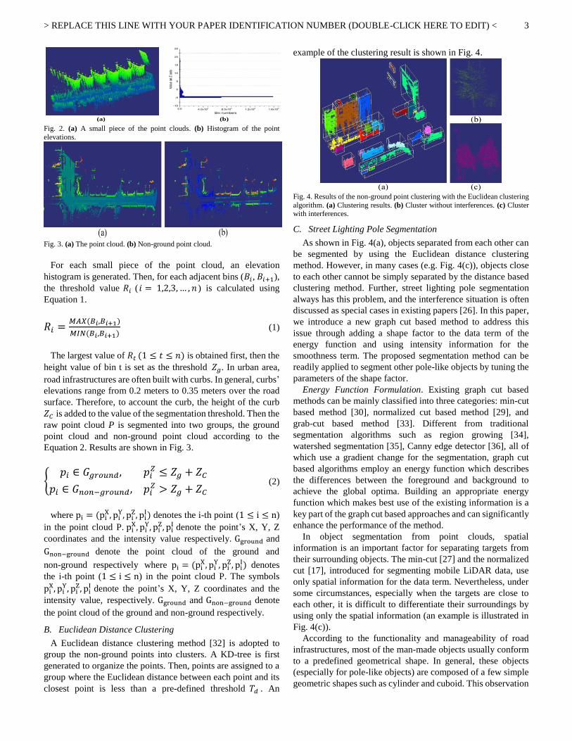
Fig. 2. (a) A small piece of the point clouds. (b) Histogram of the point

elevations.

Fig. 3. (a) The point cloud. (b) Non-ground point cloud.

For each small piece of the point cloud, an elevation

histogram is generated. Then, for each adjacent bins (𝐵𝑖 , 𝐵𝑖+1),

the threshold value 𝑅𝑖 ( 𝑖 = 1,2,3, … , 𝑛 ) is calculated using

Equation 1.

𝑅𝑖 =𝑀𝐴𝑋(𝐵𝑖,𝐵𝑖+1)

𝑀𝐼𝑁(𝐵𝑖,𝐵𝑖+1) (1)

The largest value of 𝑅𝑡 (1 ≤ 𝑡 ≤ 𝑛) is obtained first, then the

height value of bin t is set as the threshold 𝑍𝑔. In urban area,

road infrastructures are often built with curbs. In general, curbs’

elevations range from 0.2 meters to 0.35 meters over the road

surface. Therefore, to account the curb, the height of the curb

𝑍𝐶 is added to the value of the segmentation threshold. Then the

raw point cloud P is segmented into two groups, the ground

point cloud and non-ground point cloud according to the

Equation 2. Results are shown in Fig. 3.

{𝑝𝑖 ∈ 𝐺𝑔𝑟𝑜𝑢𝑛𝑑, 𝑝𝑖

𝑍 ≤ 𝑍𝑔 + 𝑍𝐶

𝑝𝑖 ∈ 𝐺𝑛𝑜𝑛−𝑔𝑟𝑜𝑢𝑛𝑑, 𝑝𝑖𝑍 > 𝑍𝑔 + 𝑍𝐶

(2)

where pi = (piX, pi

Y, piZ, pi

I) denotes the i-th point (1 ≤ i ≤ n)

in the point cloud P. piX, pi

Y, piZ, pi

I denote the point’s X, Y, Z

coordinates and the intensity value respectively. Gground and

Gnon−ground denote the point cloud of the ground and

non-ground respectively where pi = (piX, pi

Y, piZ, pi

I) denotes

the i-th point (1 ≤ i ≤ n) in the point cloud P. The symbols

piX, pi

Y, piZ, pi

I denote the point’s X, Y, Z coordinates and the

intensity value, respectively. Gground and Gnon−ground denote

the point cloud of the ground and non-ground respectively.

B. Euclidean Distance Clustering

A Euclidean distance clustering method [32] is adopted to

group the non-ground points into clusters. A KD-tree is first

generated to organize the points. Then, points are assigned to a

group where the Euclidean distance between each point and its

closest point is less than a pre-defined threshold 𝑇𝑑 . An

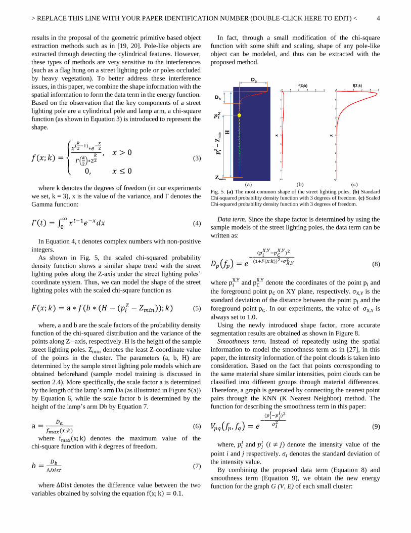
example of the clustering result is shown in Fig. 4.

Fig. 4. Results of the non-ground point clustering with the Euclidean clustering

algorithm. (a) Clustering results. (b) Cluster without interferences. (c) Cluster with interferences.

C. Street Lighting Pole Segmentation

As shown in Fig. 4(a), objects separated from each other can

be segmented by using the Euclidean distance clustering

method. However, in many cases (e.g. Fig. 4(c)), objects close

to each other cannot be simply separated by the distance based

clustering method. Further, street lighting pole segmentation

always has this problem, and the interference situation is often

discussed as special cases in existing papers [26]. In this paper,

we introduce a new graph cut based method to address this

issue through adding a shape factor to the data term of the

energy function and using intensity information for the

smoothness term. The proposed segmentation method can be

readily applied to segment other pole-like objects by tuning the

parameters of the shape factor.

Energy Function Formulation. Existing graph cut based

methods can be mainly classified into three categories: min-cut

based method [30], normalized cut based method [29], and

grab-cut based method [33]. Different from traditional

segmentation algorithms such as region growing [34],

watershed segmentation [35], Canny edge detector [36], all of

which use a gradient change for the segmentation, graph cut

based algorithms employ an energy function which describes

the differences between the foreground and background to

achieve the global optima. Building an appropriate energy

function which makes best use of the existing information is a

key part of the graph cut based approaches and can significantly

enhance the performance of the method.

In object segmentation from point clouds, spatial

information is an important factor for separating targets from

their surrounding objects. The min-cut [27] and the normalized

cut [17], introduced for segmenting mobile LiDAR data, use

only spatial information for the data term. Nevertheless, under

some circumstances, especially when the targets are close to

each other, it is difficult to differentiate their surroundings by

using only the spatial information (an example is illustrated in

Fig. 4(c)).

According to the functionality and manageability of road

infrastructures, most of the man-made objects usually conform

to a predefined geometrical shape. In general, these objects

(especially for pole-like objects) are composed of a few simple

geometric shapes such as cylinder and cuboid. This observation

(a)

(b)


4

results in the proposal of the geometric primitive based object

extraction methods such as in [19, 20]. Pole-like objects are

extracted through detecting the cylindrical features. However,

these types of methods are very sensitive to the interferences

(such as a flag hung on a street lighting pole or poles occluded

by heavy vegetation). To better address these interference

issues, in this paper, we combine the shape information with the

spatial information to form the data term in the energy function.

Based on the observation that the key components of a street

lighting pole are a cylindrical pole and lamp arm, a chi-square

function (as shown in Equation 3) is introduced to represent the

shape.

𝑓(𝑥; 𝑘) = {𝑥

(𝑘2

−1)∗𝑒

−𝑥2

𝛤(𝑘

2)∗2

𝑘2

, 𝑥 > 0

0, 𝑥 ≤ 0

(3)

where k denotes the degrees of freedom (in our experiments

we set, k = 3), x is the value of the variance, and Γ denotes the

Gamma function:

𝛤(𝑡) = ∫ 𝑥𝑡−1𝑒−𝑥𝑑𝑥∞

0 (4)

In Equation 4, t denotes complex numbers with non-positive

integers.

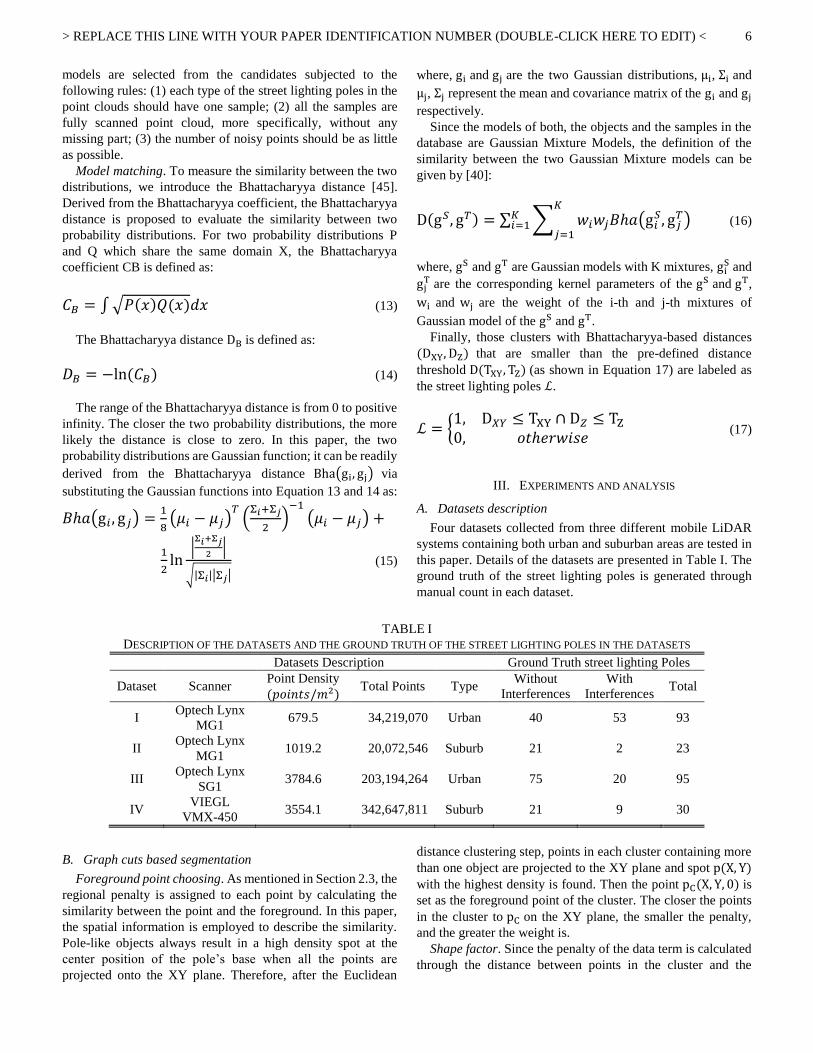
As shown in Fig. 5, the scaled chi-squared probability

density function shows a similar shape trend with the street

lighting poles along the Z-axis under the street lighting poles’

coordinate system. Thus, we can model the shape of the street

lighting poles with the scaled chi-square function as

𝐹(𝑥; 𝑘) = a ∗ 𝑓(𝑏 ∗ (𝐻 − (𝑝𝑖𝑍 − 𝑍𝑚𝑖𝑛)); 𝑘) (5)

where, a and b are the scale factors of the probability density

function of the chi-squared distribution and the variance of the

points along Z –axis, respectively. H is the height of the sample

street lighting poles. Zmin denotes the least Z-coordinate value

of the points in the cluster. The parameters (a, b, H) are

determined by the sample street lighting pole models which are

obtained beforehand (sample model training is discussed in

section 2.4). More specifically, the scale factor a is determined

by the length of the lamp’s arm Da (as illustrated in Figure 5(a))

by Equation 6, while the scale factor b is determined by the

height of the lamp’s arm Db by Equation 7.

a =𝐷𝑎

𝑓𝑚𝑎𝑥(𝑥;𝑘) (6)

where fmax(x; k) denotes the maximum value of the

chi-square function with k degrees of freedom.

𝑏 =𝐷𝑏

∆𝐷𝑖𝑠𝑡 (7)

where ∆Dist denotes the difference value between the two

variables obtained by solving the equation f(x; k) = 0.1.

In fact, through a small modification of the chi-square

function with some shift and scaling, shape of any pole-like

object can be modeled, and thus can be extracted with the

proposed method.

Fig. 5. (a) The most common shape of the street lighting poles. (b) Standard

Chi-squared probability density function with 3 degrees of freedom. (c) Scaled Chi-squared probability density function with 3 degrees of freedom.

Data term. Since the shape factor is determined by using the

sample models of the street lighting poles, the data term can be

written as:

𝐷𝑝(𝑓𝑝) = 𝑒−

(𝑝𝑖𝑋,𝑌

−𝑝𝐶𝑋,𝑌

)2

(1+𝐹(𝑥;𝑘))2∗𝜎𝑋,𝑌2

(8)

where piX,Y

and pCX,Y

denote the coordinates of the point pi and

the foreground point pC on XY plane, respectively. σX,Y is the

standard deviation of the distance between the point pi and the

foreground point pC. In our experiments, the value of σX,Y is

always set to 1.0.

Using the newly introduced shape factor, more accurate

segmentation results are obtained as shown in Figure 8.

Smoothness term. Instead of repeatedly using the spatial

information to model the smoothness term as in [27], in this

paper, the intensity information of the point clouds is taken into

consideration. Based on the fact that points corresponding to

the same material share similar intensities, point clouds can be

classified into different groups through material differences.

Therefore, a graph is generated by connecting the nearest point

pairs through the KNN (K Nearest Neighbor) method. The

function for describing the smoothness term in this paper:

𝑉𝑝𝑞(𝑓𝑝, 𝑓𝑞) = 𝑒−

(𝑝𝑖𝐼−𝑝𝑗

𝐼)2

𝜎𝐼2

(9)

where, 𝑝𝑖𝐼 and 𝑝𝑗

𝐼 (𝑖 ≠ 𝑗) denote the intensity value of the

point i and j respectively. 𝜎𝐼 denotes the standard deviation of

the intensity value.

By combining the proposed data term (Equation 8) and

smoothness term (Equation 9), we obtain the new energy

function for the graph G (V, E) of each small cluster:


5

𝐸(𝑓) =

∑ 𝑒−

(𝑝𝑖𝑋,𝑌−𝑝𝐶

𝑋,𝑌)2

(1+𝐹(𝑥;𝑘))2

∗𝜎𝑋,𝑌2

𝑝𝑖∈𝑉 + 𝜆 ∑ 𝑒−

(𝑝𝑖𝐼−𝑝𝑗

𝐼)2

𝜎𝐼2

(𝑖,𝑗)∈𝑉 (10)

where, V is the vertex set which contains all the points in the

small cluster, e−

(piX,Y−pC

X,Y)2

(1+F(x;k))2∗σX,Y2

represents the weight of the

n-link edges, and e−

(piI−pj

I)2

σI2

captures the weight of the t-link

edges. The sum of the n-link edges and the t-link edges

constitute the edge set E in the graph.

D. GMM Based Modeling and Recognition

Although the targets can be segmented out from the raw

point clouds, a few false alarms having similar shape or features

such as traffic signs and power poles can still be present in the

segmented results. Existing methods [17, 38] are either

sensitive to the noisy points or not affine-invariant. In this

paper, rather than using local features or geometric primitives

to model the targets, we introduce a statistical method which

takes the whole object into consideration through modeling

point distributions of the object.

Local coordinate system. The point distributions in XY plane

and Z axis is used to model the segments obtained by the

proposed segmentation approach and then match the segments

with the generated sample models. Thus, a unified coordinate

system is needed to guarantee the point distributions between

two different clusters sharing the same reference frame.

Therefore, a local coordinate system is established for each

segment.

For each cluster, points are first projected onto the XY plane

and the two principal components of the point sets are

calculated through the Principal Component Analysis (PCA)

[39]. The two axes of the local coordinate system L are parallel

to the first and second principal component respectively. Then

a 2D-grid is generated for the point sets, and the center

O(pCX, pC

Y) of the densest cell is set as the origin of the local

coordinate system. Finally, coordinates of the point (pix, pi

y) in

the local coordinate system L can be derived from the

coordinates (piX, pi

Y) in the global coordinate system G through

the transformation equation:

[𝑝𝑖

𝑥

𝑝𝑖𝑦] = [

𝑐𝑜𝑠𝜃 −𝑠𝑖𝑛𝜃𝑠𝑖𝑛𝜃 𝑐𝑜𝑠𝜃

] [𝑝𝑖

𝑋

𝑝𝑖𝑌 ] + [

𝑝𝐶𝑋

𝑝𝐶𝑌 ] (11)

where, 𝜃 is the angle between the first principal component of

the point sets and the X axis of the global coordinate system G.

The relationship between the two coordinate systems is

illustrated in Fig. 6, where X and Y represent the two axes of the

global coordinate system.

Fig. 6. The transformation between the global and the local coordinate system.

Fig. 7. Street lighting pole’s and tree’s point distributions on XY-plane and

Z-axis.

Mixture of Gaussian modeling. As shown in Fig. 7, different

objects in 3D space result in different point distributions. For

example, for pole-like objects, such as street lighting poles,

sharp peak can be found on the very top of the street lighting

poles in the histogram of the point distribution projected on Z

axis (the third picture in Fig.7 (a)). However, for trees the peak

is shown in the middle (the third picture in Fig.7 (b)).

Based on this fact, we represent each isolated cluster by two

point distributions, i.e. the point distributions on XY plane and

Z axis. In order to better describe the distribution of the points,

we introduce the Gaussian Mixture Model to model the

distribution. The equation of the Mixture of Gaussian is in the

following:

g = ∑ 𝑤𝑖𝐾𝑖=1 g(X; μ𝑖, Σ𝑖) (12)

where 𝑤𝑖 , 𝜇𝑖 and 𝛴𝑖 represent the weight, mean and covariance

matrix of the i-th Gaussian component of the K mixtures,

respectively.

Then, each of the clusters is defined as 𝑂 ≡ (g𝑋𝑌, g𝑍), where

g𝑋𝑌 and g𝑍 represent the Gaussian Mixture Model of the point

distribution on XY plane and Z axis respectively.

Model selection. A sample model database is generated at the

beginning. The models corresponding to the street lighting

poles are manually extracted and saved as samples. Sample


6

models are selected from the candidates subjected to the

following rules: (1) each type of the street lighting poles in the

point clouds should have one sample; (2) all the samples are

fully scanned point cloud, more specifically, without any

missing part; (3) the number of noisy points should be as little

as possible.

Model matching. To measure the similarity between the two

distributions, we introduce the Bhattacharyya distance [45].

Derived from the Bhattacharyya coefficient, the Bhattacharyya

distance is proposed to evaluate the similarity between two

probability distributions. For two probability distributions P

and Q which share the same domain X, the Bhattacharyya

coefficient CB is defined as:

𝐶𝐵 = ∫ √𝑃(𝑥)𝑄(𝑥)𝑑𝑥 (13)

The Bhattacharyya distance DB is defined as:

𝐷𝐵 = −ln (𝐶𝐵) (14)

The range of the Bhattacharyya distance is from 0 to positive

infinity. The closer the two probability distributions, the more

likely the distance is close to zero. In this paper, the two

probability distributions are Gaussian function; it can be readily

derived from the Bhattacharyya distance Bha(gi, gj) via

substituting the Gaussian functions into Equation 13 and 14 as:

𝐵ℎ𝑎(g𝑖 , g𝑗) =1

8(𝜇𝑖 − 𝜇𝑗)

𝑇(

Σ𝑖+Σ𝑗

2)

−1

(𝜇𝑖 − 𝜇𝑗) +

1

2ln

|Σ𝑖+Σ𝑗

2|

√|Σ𝑖||Σ𝑗| (15)

where, gi and gj are the two Gaussian distributions, μi, Σi and

μj, Σj represent the mean and covariance matrix of the gi and gj

respectively.

Since the models of both, the objects and the samples in the

database are Gaussian Mixture Models, the definition of the

similarity between the two Gaussian Mixture models can be

given by [40]:

D(g𝑆, g𝑇) = ∑ ∑ 𝑤𝑖𝑤𝑗𝐵ℎ𝑎(g𝑖𝑆, g𝑗

𝑇)𝐾

𝑗=1

𝐾𝑖=1 (16)

where, gS and gT are Gaussian models with K mixtures, giS and

gjT are the corresponding kernel parameters of the gS and gT,

wi and wj are the weight of the i-th and j-th mixtures of

Gaussian model of the gS and gT.

Finally, those clusters with Bhattacharyya-based distances

(DXY, DZ) that are smaller than the pre-defined distance

threshold D(TXY, TZ) (as shown in Equation 17) are labeled as

the street lighting poles ℒ.

ℒ = {1, D𝑋𝑌 ≤ TXY ∩ D𝑍 ≤ TZ

0, 𝑜𝑡ℎ𝑒𝑟𝑤𝑖𝑠𝑒 (17)

III. EXPERIMENTS AND ANALYSIS

A. Datasets description

Four datasets collected from three different mobile LiDAR

systems containing both urban and suburban areas are tested in

this paper. Details of the datasets are presented in Table I. The

ground truth of the street lighting poles is generated through

manual count in each dataset.

TABLE I

DESCRIPTION OF THE DATASETS AND THE GROUND TRUTH OF THE STREET LIGHTING POLES IN THE DATASETS

Datasets Description Ground Truth street lighting Poles

Dataset Scanner Point Density

(𝑝𝑜𝑖𝑛𝑡𝑠/𝑚2) Total Points Type

Without

Interferences

With

Interferences Total

I Optech Lynx

MG1 679.5 34,219,070 Urban 40 53 93

II Optech Lynx

MG1 1019.2 20,072,546 Suburb 21 2 23

III Optech Lynx

SG1 3784.6 203,194,264 Urban 75 20 95

IV VIEGL

VMX-450 3554.1 342,647,811 Suburb 21 9 30

B. Graph cuts based segmentation

Foreground point choosing. As mentioned in Section 2.3, the

regional penalty is assigned to each point by calculating the

similarity between the point and the foreground. In this paper,

the spatial information is employed to describe the similarity.

Pole-like objects always result in a high density spot at the

center position of the pole’s base when all the points are

projected onto the XY plane. Therefore, after the Euclidean

distance clustering step, points in each cluster containing more

than one object are projected to the XY plane and spot p(X, Y)

with the highest density is found. Then the point pC(X, Y, 0) is

set as the foreground point of the cluster. The closer the points

in the cluster to pC on the XY plane, the smaller the penalty,

and the greater the weight is.

Shape factor. Since the penalty of the data term is calculated

through the distance between points in the cluster and the


7

foreground point on XY plane, a cylinder-shaped boundary will

be formed and those points inside the boundary constitute the

foreground object. This method performs well on cylindrical

objects like mail barrels or objects that are separated from each

other. However, it fails to separate objects, such as street

lighting poles and trees, which are close to each other.

As discussed in Section 2.3, the shape information described

by a modified chi-squared function is employed in the data

term. The comparison of the graph cut based segmentation with

or without using the shape information is illustrated in Fig. 8.

Fig. 8. Examples of graph cuts based segmentation with or without shape information. The foreground and background points are colored with white and red,

respectively. The weights in the smoothness term for all experiments are all equal to 1. (a) Results of using both, the spatial and shape information in the data term.

(b) Results of using only the spatial information on XY plane with σX,Y = 0.6. (c) Results of using only the spatial information on XY plane with σX,Y = 1.0. (d)

Results of using only the spatial information on XY plane with σX,Y = 1.2. (e) Results of using only the spatial information on XY plane with σX,Y = 1.5.

In Fig. 8, five segmentation examples with the graph cut

based method are shown. The results of using both the spatial

information and shape information are illustrated in the first

row. Results using only the spatial information are shown in the

following four rows by an increasing order of the distance

deviation value on the XY plane. It can be observed from Fig.

8(b)-(d) that, as the distance deviation σX,Y increases, more

points belonging to the target (street lighting poles in this

paper) are labeled as the foreground. However, along with this,

the number of the false labeled background points is also

increased. Since the shape information is considered (Fig. 8(a)),

our method achieves the desired performance.

Table II lists the parameters used in the data term. Some of

the parameters such as the scale factors a and b, the degrees of

the freedom k used for the data term and the predefined height

of the street lighting poles H are calculated from the sample

models. The distance standard deviation σX,Y controls the

radius range of the generated cylinder for the base poles. The

larger the value, the bigger cylinder will be obtained, and more

noisy points will be included. The intensity standard deviation

σI affects the similarity evaluation of the two closest point

pairs in the smoothness term. The larger the value, more likely

the noisy points are included. The only parameters that need

tuning are the distance thresholds of the matching results.

Range thresholds for different datasets are caused by varied

shape of the street lighting poles and the fixed number of the

mixture of Gaussians employed in this paper. Street lighting

poles with more complex shapes may not be accurately

described with 2 mixtures. However, with a fixed number of the

mixtures, the algorithm performs well on the majority types of

the street lighting poles.

TABLE II

PARAMETERS USED IN THE PAPER

Parameters

Datasets 𝝈𝑿,𝒀(m) 𝝈𝑰 K 𝑻𝑿𝒀 𝑻𝒁

I

1.0 0.8 2

0.6 0.15

II 1.5 0.15 III 1.5 0.15

IV 1.5 0.3


8

The effect of the intensity information. Smoothness term in

graph cut based method measures the non-piecewise smooth

extent. Based on the assumption that neighboring points are

more likely to be assigned to the same segment, [27] make use

of the Euclidean distance between the point and its closest point

for the smoothness term. It works well on separated objects but

doesn’t work when objects are close to each other. In Fig. 9, the

performances of either using the Euclidean distance or using

the intensity information in the smoothness term are shown.

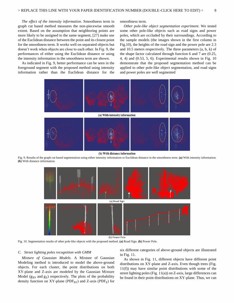
As indicated in Fig. 9, better performance can be seen in the

foreground segment with the proposed method using intensity

information rather than the Euclidean distance for the

smoothness term.

Other pole-like object segmentation experiment. We tested

some other pole-like objects such as road signs and power

poles, which are occluded by their surroundings. According to

the sample models (the images shown in the first column in

Fig.10), the heights of the road sign and the power pole are 2.3

and 10.5 meters respectively. The three parameters (a, b, k) of

the shape factor calculated through function 6 and 7 are (0.25,

4, 4) and (0.53, 5, 6). Experimental results shown in Fig. 10

demonstrate that the proposed segmentation method can be

applied to other pole-like object segmentation, and road signs

and power poles are well segmented

Fig. 9. Results of the graph cut based segmentation using either intensity information or Euclidean distance in the smoothness term. (a) With intensity information. (b) With distance information.

Fig. 10. Segmentation results of other pole-like objects with the proposed method. (a) Road Sign. (b) Power Pole.

C. Street lighting poles recognition with GMM

Mixture of Gaussian Models. A Mixture of Gaussian

Modeling method is introduced to model the above-ground

objects. For each cluster, the point distributions on both

XY-plane and Z-axis are modeled by the Gaussian Mixture

Model (gXY and gZ) respectively. The plots of the probability

density function on XY-plane (PDFXY) and Z-axis (PDFZ) for

six different categories of above-ground objects are illustrated

in Fig. 11.

As shown in Fig. 11, different objects have different point

distributions on XY-plane and Z-axis. Even though trees (Fig.

11(f)) may have similar point distributions with some of the

street lighting poles (Fig. 11(a)) on Z-axis, large differences can

be found in their point distributions on XY-plane. Thus, we can


9

differentiate the street lighting poles from trees through

matching the models between the sample street lighting poles

and the candidate objects.

Fig. 11. Above-ground object’s modeling results with GMM (In each group, the four Figures are ordered by: the raw point cloud, the projection of PDFXY on

XY-plane, the projection of PDFXY on XZ-plane, and the PDFZ on Z-axis. (a) Street lighting pole (Type 1). (b) Street lighting pole (Type 2). (c) Street lighting pole (Type 3). (d) Traffic Sign. (e) Power pole. (f) Tree. (g) Building facade. (h) Car.

Model matching. Based on the differences of the point

distributions between various objects, sample models are first

generated for each type of the street lighting poles. Then, for

each testing cluster, mixture of Gaussian models on both

XY-plane and Z-axis are generated. Finally, the model distance

between the testing objects and the training samples are

evaluated through the Bhattacharyya-based distance. The

matched ones are labeled as the street lighting poles and the

best matched label of the samples is assigned to the

corresponding object.

In order to better demonstrate the accuracy of matching, a

few other objects were chosen to match with the sample street

lighting poles, and the resultant Bhattacharyya distances are

listed in Table III. Sample street lighting poles used in this test

are shown in Fig. 12, and the testing objects are illustrated in

Fig. 13. In Table III, the distances meeting the thresholds

(shown in Table II) are shown in boldface.

As we can see from the Table III, objects with different

shapes (such as advertising board (T01, T02), building facade

(T07, T08) and traffic light (T03, T04)) show large matching

distances to the sample models. Although the cars (T05, T06)

show similar matching distances as poles on XY-plane due to

incomplete data, large distances can still be found on Z-axis.

For those pole-like objects such as power pole (T09, T10), road

sign (T11) and trees (T12-T15), similar point distributions on

the XY-plane can be readily found. However, these man-made

pole-like objects have different heights, for example, road signs

and traffic lights are usually shorter than street lighting poles,

while power poles are higher than all the other man-made

objects. Thus, they result in large distances with respect to

Z-axis from the model matching. For most of the trees, large

matching distances can be found between the training samples

and testing objects with respect to Z-axis. However, matched

false alarms (T14) still exist. So other information such as the

density of the pole center can be used to further distinguish the

street lighting poles and the false alarms. For the testing street

lighting poles (T16-T19), short distances can easily be found on

both XY-plane and Z-axis between the training samples and the

testing objects. In some case (T17), one testing street lighting

pole is matched with several samples due to their similarities.

The testing objects will be labeled by the best matched scores

(the smallest square root of the matched distance on both

XY-plane and Z-axis). For matching results of the clusters with

(T21 and T23) and without (T20 and T22) our method,

although distances (T20) with respect to Z-axis can be matched,

distances on XY-plane will not be matched for all those

unsegmented clusters. Our segmentation method successfully

separates the street lighting poles from trees and matches with

the training samples.


10

Fig. 12. Sample Street Lighting Poles.

Fig. 13. Testing examples of different above-ground objects.

D. Statistical results

In each dataset, all the clusters from segmentation are

categorized into two classes, the positive class P in which

clusters are street lighting poles and the negative class N in

which the clusters are non-street lighting poles. For each testing

cluster C, a label will be assigned after the model matching

process, and a hypothesized positive class Ph will be generated.

Four types of results: True Positive (TP), if C ∈ P ∩ Ph, True

Negative (TN), if C ∈ P̅ ∩ Ph̅, False Positive (FP), if C ∈ P ∩

Ph̅, and False Negative (FN), if C ∈ P̅ ∩ Ph, are obtained. Based

on these four categories of label results, we can evaluate the

accuracy of the recognition results comprehensively through

five quantitative indicators [43], namely True Positive Rate

(TPR = TP/(TP+FN)) which describes the probability of true

street lighting poles to be recognized, True Negative Rate

(TNR = TN/(FP+TN)) which describes the probability of

non-street lighting poles that failed to be matched with the

sample street lighting pole models, Positive Predictive Value

(PPV = TP/(TP+FP)) which reflects the probability of the true

street lighting poles recognized in all the matched results,

Negative Predictive Value (NPV = TN/(TN+FN)) which

describes the percentage of the true non-street lighting poles’

clusters in all the unmatched clusters, and accuracy (ACC =

(TP+TN)/(TP+FN+FP+TN)) which shows the overall

performance of the recognition results on both true positives

and true negatives. All the recognition results and evaluation

results are listed in Table IV.

In Table IV, for each dataset, with only one set of the

parameters (as shown in Table II), the TPR of the proposed

method reached around 90%. The overall performance of the

proposed approach in each dataset is shown in Fig. 14. Due to

the memory capacity limits of the computer for the

visualization of the large datasets, only parts of the results are

displayed for the dataset III and IV. The detected street lighting

poles, false alarms and the ground are colored in red, green and

grey respectively (Fig. 14). According to the statistical results,

false alarms are mainly small building fragments showing

similar shapes as street lighting poles (such as the ones in the

right side of Fig. 14(a)), trees (as shown in the left side of Fig.

14(a)) and short power poles (such as in Fig. 14(c)).


11

TABLE III

MODEL MATCHING RESULTS

Testing Models

Sample Models Matched

/Total S01 S02 S03 S04

D𝑋𝑌 D𝑍 D𝑋𝑌 D𝑍 D𝑋𝑌 D𝑍 D𝑋𝑌 D𝑍

Advertising

board

T01 1.009 6.703 0.803 2.068 0.961 0.481 0.967 1.051 0/2

T02 4.014 6.672 2.101 1.665 3.463 0.342 3.615 0.908

Traffic Lights T03 11.035 0.623 5.755 0.769 9.511 2.856 9.947 0.470

0/2 T04 8.377 2.001 4.381 0.892 7.233 0.086 7.558 0.281

Car T05 0.552 20.918 0.373 3.598 0.470 0.884 0.451 1.494

0/2 T06 0.577 4.149 0.413 1.132 0.509 0.229 0.498 0.798

Building

Facade

T07 1.052 0.738 0.819 0.585 1.003 0.929 1.013 0.508 0/2

T08 1.036 1.887 0.887 0.390 0.997 0.758 1.004 0.344

Power Pole T09 0.562 0.653 0.102 0.222 0.333 0.703 0.213 0.196

0/2 T10 0.467 0.460 0.116 0.158 0.290 0.557 0.213 0.146

Road Sign T11 0.676 6.616 0.095 1.579 0.378 0.223 0.222 0.625 0/1

Trees

T12 0.657 0.689 0.415 0.830 0.559 1.029 0.536 0.383

1/4 T13 0.789 1.948 0.351 1.133 0.599 0.223 0.536 0.508

T14 0.367 0.085 0.143 0.191 0.256 0.258 0.219 0.045

T15 0.363 0.812 0.096 0.578 0.227 0.131 0.176 0.189

Testing Street

Lighting Poles

T16 0.925 0.001 0.245 0.061 0.612 0.164 0.472 0.016

6/8

T17 0.377 0.088 0.076 0.066 0.223 0.051 0.154 0.116

T18 0.327 0.182 0.066 0.015 0.195 0.257 0.141 0.005

T19 0.883 0.106 0.240 0.143 0.577 0.019 0.476 0.165

T20 3.741 0.023 2.774 0.011 3.445 0.219 3.597 0.016

T21 0.768 0.050 0.752 0.049 0.527 0.091 0.569 0.066

T22 1.821 0.629 1.445 0.666 1.612 0.108 1.710 0.291

T23 0.601 0.232 0.553 0.302 0.419 0.015 0.462 0.216

TABLE IV

STATISTICAL RESULTS AND EVALUATION RESULTS OF THE FOUR DATASETS

Recognition Results Evaluation Results

Dataset Number

Without Interferences

With Interferences

TP FP Total Testing

Clusters TPR (%)

TNR (%)

PPV (%)

NPV (%)

ACC (%)

I 45 38 83 8 2026 89.25 99.59 91.21 99.48 99.11 II 20 2 22 0 1085 95.65 100 100 99.91 99.91 III 72 17 89 15 4080 93.68 99.62 85.58 99.85 99.49 IV 21 7 28 1 4114 93.33 99.98 96.55 99.95 99.93

E. Comparative studies

Graph cut based segmentation. In order to better illustrate

the performance of the proposed segmentation method, we

compared our approach with two existing graph cuts based

methods, the min-cuts based segmentation method [27] and the

normalized cuts based segmentation method [17].

In Fig.15, six samples were chosen from different data sets in

which sample 1 to 4 are from dataset I (point density: 679.5

points/m2), sample 5 to 6 are from dataset IV (point density:

3554.1 points/m2) for the performance comparison between

three graph cuts based segmentation algorithms. As shown in

Fig. 15, the normalized cuts based segmentation method

achieved acceptable results only if the foreground and

background have a similar number of points, such as shown in

Fig. 15(b)(3)-(6). The min-cuts based segmentation method

shows a better performance than the normalized cuts based

method, however with one set of parameters,

over-segmentation (Fig. 15(c)(3)-(4)) and under-segmentation

(Fig. 15(c)(5)-(6)) results can always be obtained. However,

with one set of the parameters, the proposed segmentation

method shows better performance (Fig. 15(d)).


12

Fig. 14. The overall performance of each dataset tested in this paper (the detected street lighting poles, false alarms and the ground are colored in red, green and grey

respectively). (a) Dataset I. (b) Dataset II. (c) Dataset III. (d) Dataset IV.

Fig. 15. Comparison of the performance of three graph cuts based segmentation methods (Foreground and background points are colored as white and red

respectively). (a) Raw point cloud of street lighting pole with interferences. (b) Segmentation results of the normalized cut method. (c) Segmentation results of the min-cuts based method. (d) Segmentation results of the proposed method.


13

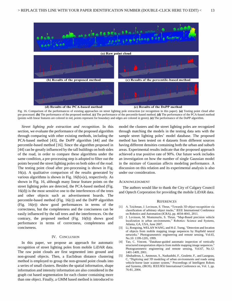
Fig. 16. Comparison of the performances of existing approaches on street lighting pole extraction (or recognition in this paper). (a) Testing point cloud after

pre-processed. (b) The performance of the proposed method. (c) The performance of the percentile-based method. (d) The performance of the PCA-based method (points with linear features are colored in red, points represent for boundary and edges are colored in green). (e) The performance of the DoPP algorithm.

Street lighting pole extraction and recognition. In this

section, we evaluate the performance of the proposed algorithm

through comparing with other existing methods, including the

PCA-based method [43], the DoPP algorithm [44] and the

percentile-based method [16]. Since the algorithm proposed in

[44] can be greatly influenced by the tall buildings on both sides

of the road, in order to compare these algorithms under the

same condition, a pre-processing step is adopted to filter out the

points beyond the street lighting poles on both sides of the road.

The testing point cloud after pre-processing is shown in Fig.

16(a). A qualitative comparison of the results generated by

various algorithms is shown in Fig. 16(b)-(e), respectively. As

shown in Fig. 16, although many linear feature points on the

street lighting poles are detected, the PCA-based method (Fig.

16(d)) is the most sensitive one to the interferences of the trees

and other objects such as advertisement boards. The

percentile-based method (Fig. 16(c)) and the DoPP algorithm

(Fig. 16(e)) show good performances in terms of the

correctness, but the completeness and the conciseness can be

easily influenced by the tall trees and the interferences. On the

contrary, the proposed method (Fig. 16(b)) shows good

performance in terms of correctness, completeness and

conciseness.

IV. CONCLUSION

In this paper, we propose an approach for automatic

recognition of street lighting poles from mobile LiDAR data.

The raw point clouds are first segmented into ground and

non-ground objects. Then, a Euclidean distance clustering

method is employed to group the non-ground point clouds into

a series of small clusters. Besides the spatial information, shape

information and intensity information are also considered in the

graph cut based segmentation for each cluster containing more

than one object. Finally, a GMM based method is introduced to

model the clusters and the street lighting poles are recognized

through matching the models in the testing data sets with the

sample street lighting poles’ model database. The proposed

method has been tested on 4 datasets from different sources

having different densities containing both the urban and suburb

areas. Experimental results indicate that the proposed approach

achieved a true positive rate of 90%. Our future work includes

an investigation on how the number of single Gaussian model

in the mixture of Gaussian affects modeling performance. A

discussion on this relation and its experimental analysis is also

under our consideration.

ACKNOWLEDGMENT

The authors would like to thank the City of Calgary Council

and Optech Corporation for providing the mobile LiDAR data.

REFERENCES

[1] A. Teichman, J. Levinson, S. Thrun, “Towards 3D object recognition via

classification of arbitrary object tracks,” IEEE International Conference on Robotics and Automation (ICRA), pp. 4034-4041, 2011.

[2] J. Levinson, M. Montemerlo, S. Thrun, “Map-Based precision vehicle

localization in urban environments,” Robotics: Science and Systems, Atlanta, GA, USA, June 2007.

[3] Li, Rongxing, WELAN WANG, and H-Z. Tseng, "Detection and location

of objects from mobile mapping image sequences by Hopfield neural networks." Photogrammetric engineering and remote sensing, Vol.65,

No.10: 1199-1205, 1999.

[4] Tao, C. Vincent. "Database-guided automatic inspection of vertically structured transportation objects from mobile mapping image sequences."

Photogrammetric engineering and remote sensing, Vol.67, No.12:

1401-1409, 2001. [5] Abuhadrous, I., Ammoun, S., Nashashibi, F., Goulette, F., and Laurgeau,

C, “Digitizing and 3D modeling of urban environments and roads using

vehicle-borne laser scanner system,” Proceedings of Intelligent Robots and Systems, (IROS). IEEE/RSJ International Conference on, Vol. 1, pp.

76-81, 2004.


14

[6] Aleksey Boyko, and Thomas Funkhouser, “Extracting roads from dense

point clouds in large scale urban environment,” ISPRS Journal of Photogrammetry and Remote Sensing, Vol. 66, No. 6 pp. S2-S12, 2011.

[7] Wende Zhang, “LiDAR-Based road and road-edge detection,” IEEE

Intelligent Vehicles Symposium, San Diego, CA, USA, pp. 845-848, JUN. 2010.

[8] Kay Ch. Fuerstenberg, Klaus C.J. Dietmayer, and Volker Willhoeft,

“Pedestrian recognition in urban traffic using a vehicle based multilayer laserscanner,” Intelligent Vehicle Symposium, IEEE. Vol. 1, pp. 31-35,

2002.

[9] Rakusz, T. Lovas and A. Barsi, “LIDAR-Bascd Vehicle Segmentation,” in International Conference on Photgrammetry and Remote Sensing,

Istanbul, Turkey, 2004.

[10] B.J. Li, Q.Q. Li, W.Z. Shi and F.F. Wu, “Feature Extraction And Modeling Of Urban Building From Vehicle-Borne Laser Scanning Data,”

International Archives of Photogrammetry, Remote Sensing and Spatial

Information Sciences, pp. 934-940, 2004. [11] Pu Shi and George Vosselman, “Knowledge based reconstruction of

building models from terrestrial laser scanning data,” ISPRS Journal of

Photogrammetry and Remote Sensing, Vol. 64, No. 6, pp. 575-584, 2009. [12] Huang Zuowei, Xiang Chi, and Fang Liu, “A methodology for extraction

building facades from VLS,” Digital Manufacturing and Automation

(IDCMA), 2012 Third International Conference on. IEEE, pp. 77-80, 2012.

[13] J. Martínez, Soria-Medina A, Arias P, et al., “Automatic processing of

terrestrial laser scanning data of building facades,” Automation in Construction, Vol. 22, pp. 298-305, 2012.

[14] Wang, R., F. Ferrie, and J. Macfarlane, “A Method for Detecting Windows from Mobile LiDAR Data,” Photogrammetric Engineering and

Remote Sensing, Vol. 78, No. 11, pp.1129-1140, 2012.

[15] Brenner, C., “Extraction of Features from Mobile Laser Scanning Data for Future Driver Assistance Systems,” Advances in GIScience, Lecture

Notes in Geoinformation and Cartography. Springer, pp. 25–42, 2009.

[16] Shi Pu, M.R., George Vosselman, Sander Oude Elberink, “Recognizing basic structures from mobile laser scanning data for road inventory

studies,” ISPRS Journal of Photogrammetry and Remote Sensing, 66(6):

pp. S28-S39,2011. [17] Yongtao Yu, Jonathan Li, Haiyan Guan, Cheng Wang and Jun Yu,

“Semiautomated Extraction of Street Light Poles From Mobile LiDAR

Point-Clouds,” IEEE Trans. Geosci. Remote Sens., Vol. 53, no. 3, pp. 1374-1386, 2015.

[18] Nurunnabi, A., et al., “Robust Segmentation in Laser Scanning 3D Point

Cloud Data,” 2012 International Conference on Digital Image Computing Techniques and Applications, 2012.

[19] Paul J.Besl and Ramesh C. Jain, “Segmentation through variable-order

surface fitting,” Pattern Analysis and Machine Intelligence, IEEE Transactions on, 10(2): pp. 167-192. 1988.

[20] Rabbani, T., F.v.d. Heuvel, and G. Vosselmann, “Segmentation of point clouds using smoothness constraint,” International Archives of

Photogrammetry, Remote Sensing and Spatial Information Sciences,

36(5): pp. 248-253. 2006. [21] Lehtomäki M, J.A., Hyyppä J, et al, “Detection of vertical pole-like

objects in a road environment using vehicle-based laser scanning data,”

Remote Sensing, 2(3): pp. 641-664, 2010. [22] Rusu R B, B.N., Marton Z C and Micheal Beetz, “Close-range scene

segmentation and reconstruction of 3D point cloud maps for mobile

manipulation in domestic environments,” in IEEE/RSJ International Conference on Intelligent Robots and Systems. pp. 1-6. 2009.

[23] Ee Hui Lim, D.S., “Multi-scale conditional random fields for

over-segmented irregular 3D point-clouds classification,” in Computer

Vision and Pattern Recognition Workshops. pp. 1-7. 2008.

[24] Ee Hui Lim, D.S., “3D terrestrial lidar classifications with super-voxels

and multi-scale conditional random fields,” Computer-Aided Design, 41(10): pp. 701-710. 2009.

[25] Aijazi A K, C.P., Trassoudaine L., “Segmentation based classification of

3D urban point clouds: a super-voxel based approach with evaluation,” Remote Sensing, 5(4): pp. 1624-1650. 2013.

[26] Bisheng Yang, Z.D., Gang Zhao, Wenxia Dai, “Hierarchical extraction of

urban objects from mobile laser scanning data,” ISPRS Journal of Photogrammetry and Remote Sensing, 99: pp. 45-57. 2015.

[27] Aleksey Golovinskiy, T.F., “Min-Cut Based Segmentation of Point

Clouds,” in Computer Vision Workshops (ICCV Workshops), 2009 IEEE 12th International Conference on: Kyoto. pp. 39-46. 2009.

[28] Hiroki Yokoyama, Hiroaki Date, Satoshi Kanai and Hiroshi Takeda,

“Detection and classification of Pole-like objects from Mobile Laser

Scanning data of urban environments,” International Journal of

CAD/CAM, Vol. 13, No. 2, pp.31-40, 2013. [29] Jianbo Shi and Jitendra Malik, “Normalized cuts and image

segmentation,” Pattern Analysis and Machine Intelligence, IEEE

Transactions on, 22(8): pp. 888 - 905. 2000. [30] Yuri Boykov, Veksler, O., Z. R., “Fast approximate energy minimization

via graph cuts,” Pattern Analysis and Machine Intelligence, IEEE

Transactions on, 23(11): pp. 1222 - 1239. 2001. [31] Yu Y, Li J, Guan H, Jia F, Wang C, “Three-dimensional object matching

in mobile laser scanning point clouds,” IEEE Geoscience and Remote

Sensing Letters, 12(3): pp. 492-496, 2015. [32] Rusu, R.B., “Semantic 3D Object Maps for Everyday Manipulation in

Human Living Environments,” PhD Thesis, TECHNISCHE

UNIVERSITÄT MÜNCHEN: Munich, Germany. 2009. [33] Carsten Rother, V.K., Andrew Blake, “‘GrabCut’ — Interactive

Foreground Extraction using Iterated Graph Cuts,” ACM Transactions on

Graphics (TOG), 23(3): pp. 309-314. 2004. [34] R Adams, L Bischof, “Seeded region growing,” IEEE Transactions on

Pattern Analysis and Machine Intelligence 16(6), pp. 641–647, 1994.

[35] L Vincent, P Soille, “Watersheds in digital spaces: an efficient algorithm based on immersion simulations,” IEEE Transactions on Pattern Analysis

and Machine Intelligence. 13(6), pp. 583–598 1991.

[36] J. Canny, “Computational approach to edge detection,” IEEE Transactions on Pattern Analysis and Machine Intelligence 8(6), pp. 679–

698 1986.

[37] Veksler, O., “Star shape prior for graph-cut image segmentation,” in Computer Vision – ECCV. Springer Berlin Heidelberg. pp. 454-467.

2008. [38] M. Körtgen, G. J. Park, M. Novotni, and R. Klein, “3D shape matching

with 3D shape contexts,” in Proc. 7th Central Eur. Semin. Comput.

Graph, Budmerice, Slovakia, vol. 3, pp. 5–17. 2003. [39] Jolliffe, I.T., Principal Component Analysis. 2 ed. Springer Series in

Statistics: Springer-Verlag New York. 2002.

[40] G. Sfikas, C. Constantinopoulos, A. Likas, and N.P. Galatsanos, “An analytic distance metric for Gaussian mixture models with application in

image retrieval,” Artificial Neural Networks: Formal Models and Their

Applications–ICANN, Springer, vol. 3697, pp. 835-840, 2005. [41] K. Fukunaga, “Introduction to statistical pattern recognition,” second

edition, Academic Press Incorporation, San Diego, CA, USA, 1990.

[42] Powers, D.M.W., “Evaluation: from precision, recall and F-measure to ROC, informedness, markedness and correlation,” Journal of Machine

Learning Technologies. 2(1): pp. 37-63. 2011.

[43] Sherif Ibrahim El-Halawany, D.D.L., “Detection of road poles from mobile terrestrial laser scanner point cloud,” in

Multi-Platform/Multi-Sensor Remote Sensing and Mapping (M2RSM).

International Workshop on. IEEE. pp. 1-6. 2011. [44] Y. Hu, X.L., J. Xie, and L. Guo. “A novel approach to extracting street

lamps from vehicle-borne laser data,” Geoinformatics, 19th International

Conference on. IEEE. Shanghai, China. pp. 1-6. 2011. [45] A. Bhattacharyya. “On a measure of divergence between two multinomial

populations,” The Indian Journal of Statistics. 7(4): pp. 401-406. 1946.

Han Zheng received the B.S. and M.S.

degree in geodesy and geomatics

engineering from Wuhan University,

Wuhan, China, in 2011 and 2013

respectively. Now he is working toward

his second master degree in digital image

system in the Department of Geomatics

Engineering from the University of

Calgary, Calgary, AB, Canada.

His current research interests include laser measurement

application, computer vision, digital image processing, and

object recognition from three dimensional point clouds.

http://www.ucalgary.ca/rswang/files/rswang/windowdetectionfrommobilelidardata_accepted.pdf

http://www.ucalgary.ca/rswang/files/rswang/windowdetectionfrommobilelidardata_accepted.pdf


15

Ruisheng Wang joined the Department of

Geomatics Engineering at the University

of Calgary as an Assistant Professor in

2012. Prior to that, he worked as an

industrial researcher at HERE Maps in

Chicago, USA since 2008. Dr. Wang holds

a Ph.D. in Electrical and Computer

Engineering from the McGill University, a

M.Sc.E.in Geomatics Engineering from the University of New

Brunswick, and a B.Eng. in Photogrammetry and Remote

Sensing from the Wuhan University, respectively. His current

research interests include Geomatics and computer vision.

Sheng Xu received the M.S. degree in

computer science and technology from

Nanjing Forestry University, Nanjing,

China, in 2010. He is currently pursuing

the Ph.D. degree in the Department of

Geomatics Engineering from the

University of Calgary, Calgary, AB,

Canada.

His current research interests include computer vision, mobile

LiDAR data processing, and information extraction from 3D

point clouds.

recognizing street lighting poles from mobile lidar data · mobile lidar is a newly emerging...

Documents