recognition of facial expressions using local mean … · ... we propose a novel appearance based...
TRANSCRIPT
Correspondence to: <[email protected]>
Recommended for acceptance by <Angel Sappa>
http://dx.doi.org/10.5565/rev/elcvia.1058
ELCVIA ISSN: 1577-5097
Published by Computer Vision Center / Universitat Autonoma de Barcelona, Barcelona, Spain
Electronic Letters on Computer Vision and Image Analysis 16(1):54-67, 2017
Recognition of Facial Expressions using Local Mean Binary Pattern
Mahesh Goyani* and Narendra Patel+
* Department of Computer Engineering, Charotar University of Science and Technology, Changa, India
+ Department of Computer Engineering , BVM Engineering College, V.V.Nagar, India
Received 12th Feb 2017; accepted 22nd May 2017
Abstract
In this paper, we propose a novel appearance based local feature descriptor called Local Mean Binary Pattern
(LMBP) for facial expression recognition. It efficiently encodes the local texture and global shape of the face.
LMBP code of a pixel is produced by weighting the thresholded neighbor intensity values with respect to mean
of 3 3 patch. LMBP produces highly discriminative code compared to other state of the art methods. The micro
pattern is derived by thesholding on mean of the patch, and hence it is robust against illumination and noise
variations. An image is divided into M N regions and feature descriptor is derived by concatenating LMBP
distribution of each region. We also propose a novel template matching strategy called Histogram Normalized
Absolute Difference (HNAD) for comparing LMBP histograms. Rigorous experiments prove the effectiveness
and robustness of LMBP operator. Experiments also prove the superiority of HNAD measure over well-known
template matching methods such as L2 norm and Chi-Square. We also investigated LMBP for expression
recognition in low resolution. The performance of the proposed approach is tested on well-known datasets CK,
JAFFE, and TFEID.
Key Words: Local Binary Pattern, Local Direction Pattern, Local Mean Binary Pattern, Histogram
Normalized Absolute Difference, Support Vector Machine.
1 Introduction
Facial expression plays a vital role in communicating emotions and intentions [1]. Visual clues and
information lead towards a better understanding in a conversation. Application area of FER covers a broad
spectrum, including grading of physical pain, smile detection [2], [3], [4], driver fatigue detection [5], patient
pain assessment [6], video indexing, robotics and virtual reality [7], depression detection [8] etc. Mental state
is imitated on the face in the form of various expressions; affective computing models them in an appropriate
computer actions [9]. Interpretation of facial expression through the machine can become a driving force for
the future automation interfaces such as car driving, robotics, driver alert systems, human-computer
interfaces etc. [7], [10].
Investigation of the Physiognomy and facial expression dates to the era of Aristotle (4th century).
Physiognomy is the Greek word, in which physis means “nature” and gnom means “judge”. It corresponds to
judging people’s character from their external appearance, especially from the face [11]. In 1872, the first
Mahesh Goyani et al. / Electronic Letters on Computer Vision and Image Analysis 16(1):54-67, 2017 55
preliminary experiment on facial expression was conducted by Charles Darvin, that had a direct influence on
modern FER research during that time. He mentioned the generality of facial expressions across human and
animals in his well-known book "The Expression of the Emotions in Man and Animal" [12]. He observed
how humans and animals exhibit the common characteristics while expressing their emotions. Both have a
tendency of showing their ocular muscles and tighten their teeth when they are in anger state. Darvin’s claim
of universality in expression was reinforced by the series of cross cultural experiments conducted by Ekman
and Friesen in 1971 [13]. They postulated a range of expressions into six judgmental classes, which are
anger, disgust, fear, happy, sad and surprise. Most of the research on facial expression is centered around
detecting these basic six expressions.
In this paper, we propose a novel appearance based local face descriptor called Local Mean Binary
Pattern. LMBP code is obtained by deriving LBP code of mean centered patch of size 3 3. Consequently,
this approach is robust against non-monotonic gray level change and random noise. LMBP efficiently
characterizes the local intensity variation and structural information. We also present a novel template
matching technique called Histogram Normalized Absolute Difference (HNAD) for matching the LMBP
histograms. Proposed measure normalizes the absolute difference of two histogram values by the union of
histograms. Experiments show that HNAD outperforms the customary template matching techniques like L2
norm and Chi-square. The discriminative capability of LMBP is also investigated for low-resolution facial
expression recognition. Results show the stability of over a wide range of low-resolution images, which
motivates the use of LMBP for real world applications.
Rest of the paper is organized as follows: State of the art methods have been studied in section 2. A brief
review on local statistical operators like Local Binary Pattern (LBP) and Local Directional Pattern (LDP) is
presented in Section 3. The proposed appearance based operator Local Mean Binary Pattern is introduced in
Section 4. Section 5 describes the novel template matcher HNAD along with experimental setup and facial
expression datasets. Optimal parameter selection, result analysis and expression recognition in low resolution
are presented in section 6. Finally, the work is summarized in Section 7.
2 State of the Art Methods
There are commonly two approaches for facial feature extraction: geometric feature based methods and
appearance feature based methods [7], [9], [14], [15]. Many modern facial expression recognition systems
utilize the vector of position and relation of certain facial key points as a feature descriptor. Such systems are
referred as geometry based systems. The facial key points, whose position is localized are known as fiducial
points. Typically, fiducial points are positioned along the nose, lip, eye and eyebrow. The motivation for
using geometry based systems is that each expression affects the relative position of such fiducial points.
Appearance or texture based analysis of the image is very useful in applications at different levels [16]. The
texture is the visual property which characterizes the surface by means of variations in shape, illumination,
reflectance, shadow, absorption etc. In appearance-based methods, certain filters or kernel functions are
applied on the face to extract a feature vector. Appearance/texture features are more suitable for capturing
subtle appearance changes (e.g. wrinkles) of the face, while geometric features are more capable of
representing the shape and location information of facial components (e.g. mouth, eye, nose etc.). Geometry
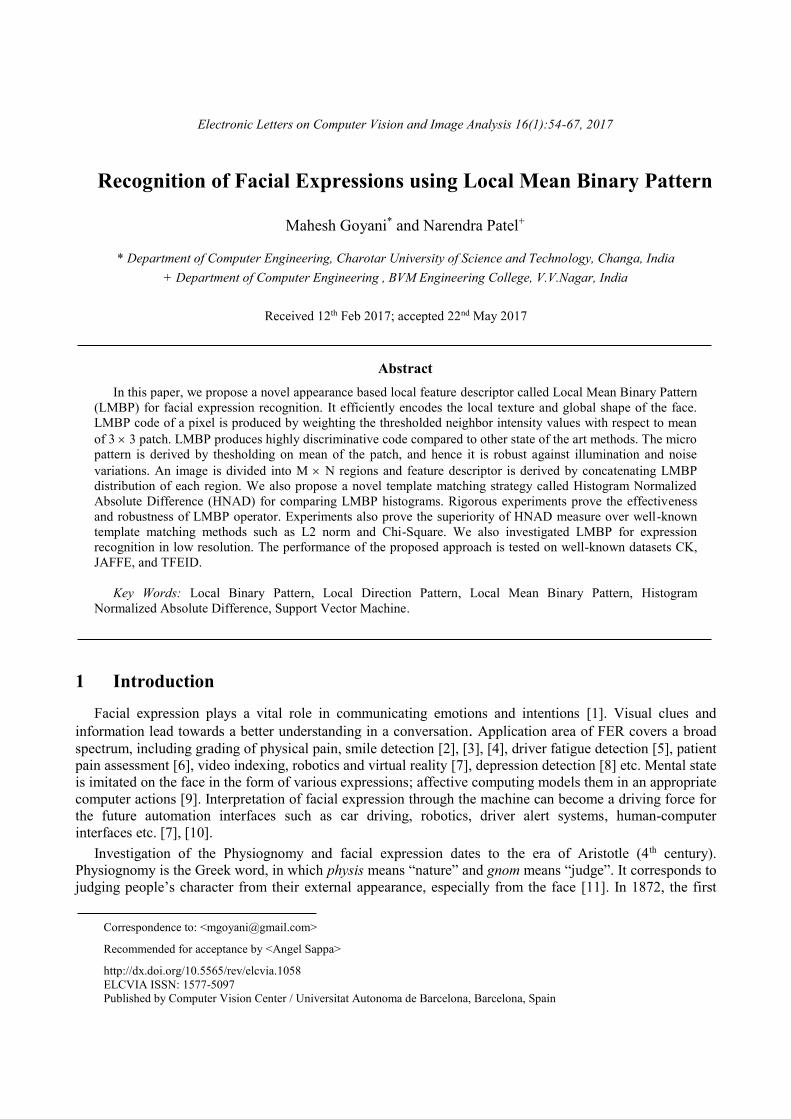
and appearance based features are depicted in Figure 1.
Fig. 1. Illustration of geometric (left) and appearance (right) features
56 Mahesh Goyani et al. / Electronic Letters on Computer Vision and Image Analysis 16(1):54-67, 2017
Based on the region of operation, facial extraction methods are further classified into global and local.
Global methods operate on entire image and hence they are also known as holistic methods. Optical flow
[17], [18], Eigenface [19], Fisherface [20], Independent Component Analysis (ICA) [21] are few of the
widely used holistic methods. Even though these methods have been significantly used and explored, local
descriptors have gained the attention of researchers because of their robustness and invariance property.
Local feature extraction methods operate on a small neighbourhood of the pixel. Feature descriptor is
obtained by collecting features computed locally. Local Binary Pattern (LBP) [22], multi-resolution LBP
[23], Local Directional Pattern (LDP) [24], Gabor filter [25], Local Gabor Binary Pattern (LGBP) [10] are
some of the well-studied local feature extraction methods.
Comprehensive and widely cited surveys by Samal and Lyengar [26], Pantic and Rothkrantz [7] and Fasel
and Luetin (2003) [8] are available that perform an in-depth study of the published work from 1990 to 2001.
Recent advancements in the 21st century are surveyed by Tian et al. [27], Zeng et al. [8], Dailey et al. [28],
Murtaza et al. [29] and Corneanu et al. [14].
3 Revisiting Local Statistical Operators
The two important aspects of facial expression recognition comprise facial representation and design of
the classifier. Facial representation refers to finding a set of features that can effectively characterize the face
image. The optimal feature should maximize the intra-class similarity and minimize the interclass similarity
[30]. The success of an appropriate classifier ultimately depends on an effective facial representation, which
can lead to better recognition rate.
3.1 Local Binary Pattern
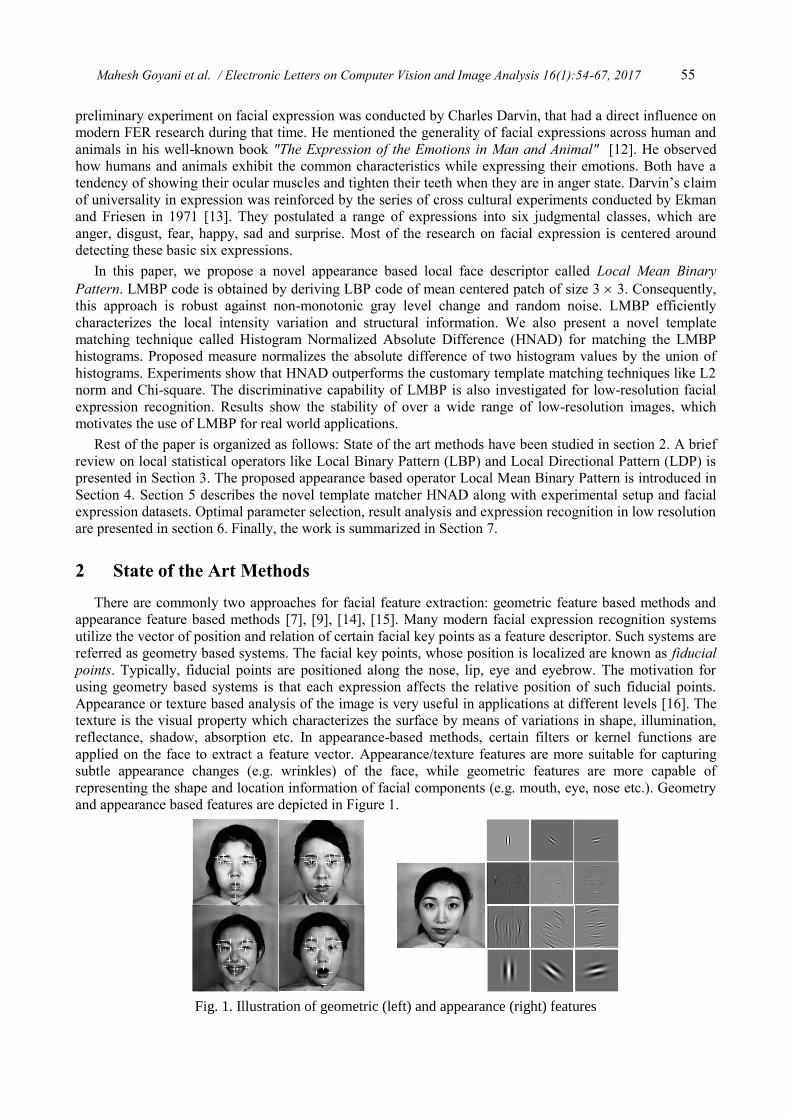
Local binary pattern is comprehensively studied powerful texture analysis descriptor. In 1996, Ojala et al.
[22] proposed LBP for analysing macro and micro patterns of the image. It encodes micro patterns in the
local neighbourhood of the pixel using knowledge of neighbour pixel intensity. LBP is invariant to changes
in monotonic gray level. LBP code is generated by weighting the thresholded P neighbours by the decimal
values. LBP code for the center pixel (xc, yc) is computed as,
0,0
0,1)(,)(*2),(
1
0
,x
xxSiiSyxLBP
P
n
cn
n
ccRP
Where, in denotes the gray value of equally spread out P neighbours on the perimeter of radius R with
respect to center (xc, yc), and ic is the gray value of center pixel. Binary value assigned by function S(.) over
P bits is weighted by the decimal value, which gives the LBP code for center pixel. Figure 2 illustrates the
steps for LBP code generation.
Fig. 2. LBP operator to compute the LBP code for P bits and radius R
Many variants of LBP are proposed to make it more robust. Ojala et al. [31] introduced uniform binary
pattern to reduce the feature dimensions. By combining Gabor filtering with LBP, Local Gabor Binary
Patterns (LGBP) [32] was proposed to extend LBP to multiple resolutions and orientations. Shan et al. [30]
presented boosted LBP based approach to extract most discriminative LBP features. They also extend the
experiment for low-resolution images. To further reduce the computation, Hablani et al. [33] employed LBP
on prominent regions of the face. LBP histograms of eyes, mouth, nose are concatenated to form the final
feature vector.
3.2 Local Directional Pattern

Mahesh Goyani et al. / Electronic Letters on Computer Vision and Image Analysis 16(1):54-67, 2017 57
Jabid et al. [24] present a Local Direction Pattern (LDP) descriptor for facial representation. LDP derives
8-bit binary pattern by encoding edge response value in 8 directions using Kirsch edge detector. Kirsch
detects directional response more accurately compared to Prewitt or Sobel edge detectors. Though Kirsch
operator is robust, it is computationally demanding as it uses eight different masks to compute response in
each direction. Masks used to compute LDP are shown in Figure 3.
333
305
355
333
303
555
333
503
553
533
503
533
North West M0 North M1 North East M2 East M3
553
503
333
555
303
333
355
305
333
335
305
335
South East M4 South M5 South West M6 West M7
Fig. 3. Kirsch edge detector masks Mi-th mask generates mi response, where i = 0,1,…,7. The response of eight masks is collected in a 3 3
matrix as displayed in Figure 4. Neighbor responses are thresholded with respect to mk-th directional
response. The value of k is chosen by rigorous experiments. LBP of these responses gives the LDP code for
center pixel. Histogram of these LDP values is used as a feature descriptor.
Fig. 4. Generation of LDP code
Given the center pixel and 8-Kirsch masks, eight direction edge response mi is computed for i=0, 1…, 7.
LDP code is computed as,
0,0
0,1)(,)(*2),(
7
0 x
xxSmmSyxLDP
n
kn
n
cck
Where mk is the k-th most significant directional response. Edge response is more stable than the intensity
value, sometimes LDP generates same code even though the LBP code is different.
4 Local Mean Binary Pattern
LBP is simple and efficient but it is sensitive to noise and non-monotonic gray level changes. LDP uses
fixed eight masks to measure edge response, so it cannot be stretched to operate at multi-scale or
multiresolution. In addition, computing responses in eight directions for each pixel is also computationally
intensive. Both the issues, robustness and computation cost are handled by LMBP operator with ease. It
assigns an eight-bit binary code to each pixel, which represents the local structure. Multiscale modelling of
LMBP is very similar to that of LBP. It may with ease be improved to work at different scale and resolution.
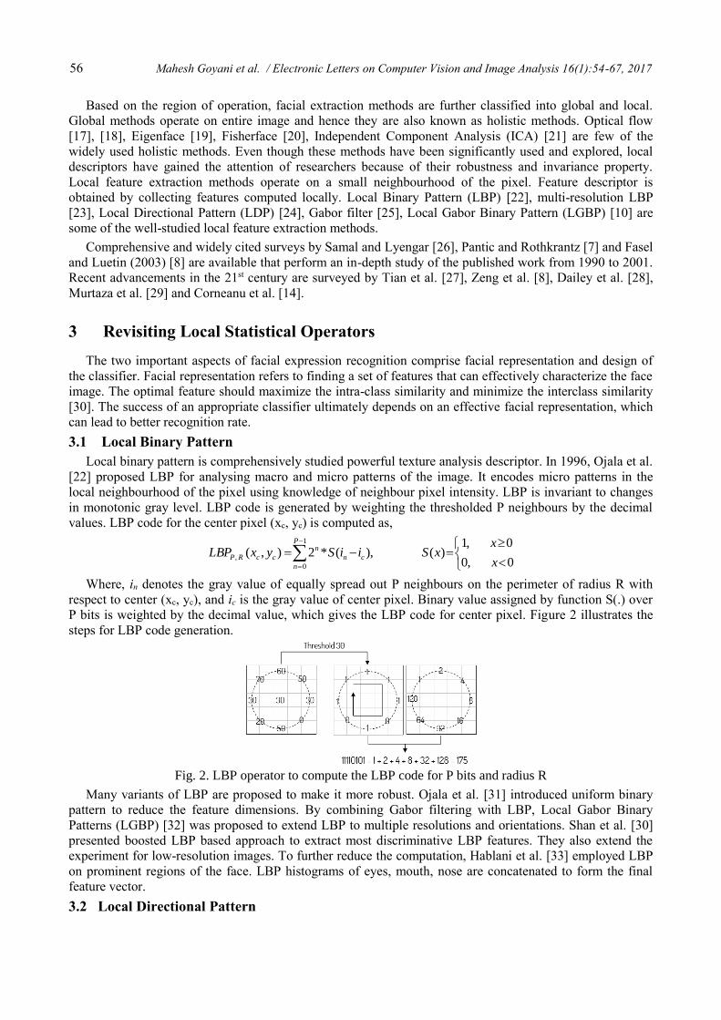
In proposed LMBP, the mean value of 3 3 neighbourhood is compared with eight neighbour values. LMBP
code of center pixel (xc, yc) is computed as follow:
0,0
0,1)(,)(*2),(
7
0 x
xxSiiSyxLMBP
n
mn
n
cc
Where, in is the intensity of neighbour of center pixel (xc, yc), and im is the mean intensity of 3 3 image
patch. LMBP of code is resilient to noise and illumination compared to normal LBP operator. The mean of
patch suppresses the effect of both, noise and illumination, by diluting the intensity variation. And still, the
structural information of the original image is preserved. It provides the stability to generated LMBP code.
Working of basic LMBP operator is portrayed in Figure 5.
58 Mahesh Goyani et al. / Electronic Letters on Computer Vision and Image Analysis 16(1):54-67, 2017
Fig. 5. The procedure of computing LMBP code: (a). Compute mean of 3 3 patches, (b). Find mean
centered patch, (c). The thresholded output of (b), (d). Weight matrix to be applied to (c), (e). Final masked
patch used to derive LHMBP value. The mean value of the patch is subtracted from eight neighbours (Figure 5(b)). Non-negative neighbours
are assigned bit 1, and negative neighbours are assigned bit 0 (Figure 5(c)). The weight matrix shown in
Figure 5(d) is applied to thresholded patch. Summation of masked output is the LMBP code of center pixel.
4.1 Robustness of LMBP
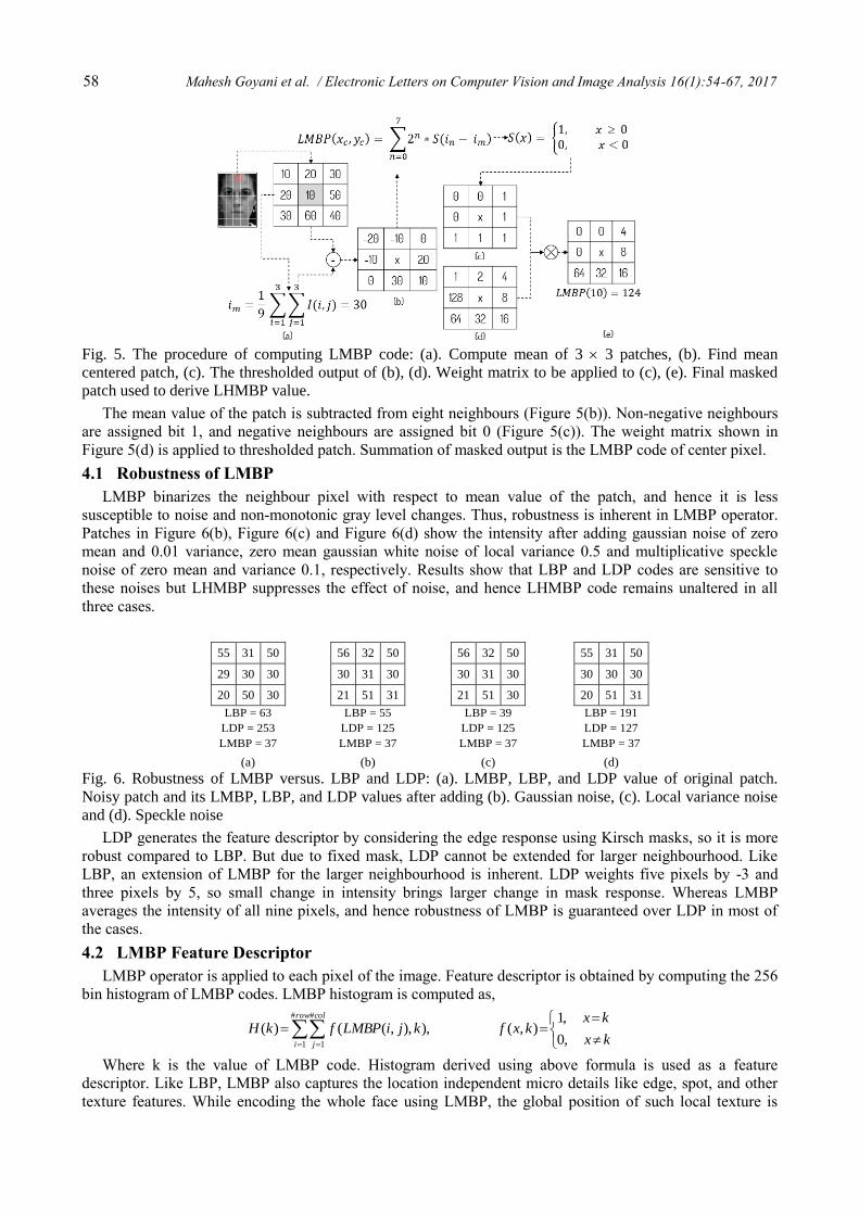
LMBP binarizes the neighbour pixel with respect to mean value of the patch, and hence it is less
susceptible to noise and non-monotonic gray level changes. Thus, robustness is inherent in LMBP operator.
Patches in Figure 6(b), Figure 6(c) and Figure 6(d) show the intensity after adding gaussian noise of zero
mean and 0.01 variance, zero mean gaussian white noise of local variance 0.5 and multiplicative speckle
noise of zero mean and variance 0.1, respectively. Results show that LBP and LDP codes are sensitive to
these noises but LHMBP suppresses the effect of noise, and hence LHMBP code remains unaltered in all
three cases.
55 31 50
29 30 30
20 50 30
56 32 50
30 31 30
21 51 31
56 32 50
30 31 30
21 51 30
55 31 50
30 30 30
20 51 31
LBP = 63
LDP = 253
LMBP = 37
LBP = 55
LDP = 125
LMBP = 37
LBP = 39
LDP = 125
LMBP = 37
LBP = 191
LDP = 127
LMBP = 37
(a) (b) (c) (d)
Fig. 6. Robustness of LMBP versus. LBP and LDP: (a). LMBP, LBP, and LDP value of original patch.
Noisy patch and its LMBP, LBP, and LDP values after adding (b). Gaussian noise, (c). Local variance noise
and (d). Speckle noise
LDP generates the feature descriptor by considering the edge response using Kirsch masks, so it is more
robust compared to LBP. But due to fixed mask, LDP cannot be extended for larger neighbourhood. Like
LBP, an extension of LMBP for the larger neighbourhood is inherent. LDP weights five pixels by -3 and
three pixels by 5, so small change in intensity brings larger change in mask response. Whereas LMBP
averages the intensity of all nine pixels, and hence robustness of LMBP is guaranteed over LDP in most of
the cases.
4.2 LMBP Feature Descriptor
LMBP operator is applied to each pixel of the image. Feature descriptor is obtained by computing the 256
bin histogram of LMBP codes. LMBP histogram is computed as,
row
i
col
j kx
kxkxfkjiLMBPfkH
#
1
#
1 ,0
,1),(),),,(()(
Where k is the value of LMBP code. Histogram derived using above formula is used as a feature
descriptor. Like LBP, LMBP also captures the location independent micro details like edge, spot, and other
texture features. While encoding the whole face using LMBP, the global position of such local texture is
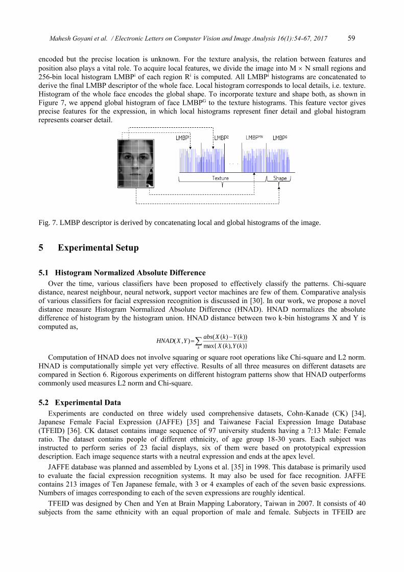
Mahesh Goyani et al. / Electronic Letters on Computer Vision and Image Analysis 16(1):54-67, 2017 59
encoded but the precise location is unknown. For the texture analysis, the relation between features and
position also plays a vital role. To acquire local features, we divide the image into M N small regions and
256-bin local histogram LMBPi of each region Ri is computed. All LMBPi histograms are concatenated to
derive the final LMBP descriptor of the whole face. Local histogram corresponds to local details, i.e. texture.
Histogram of the whole face encodes the global shape. To incorporate texture and shape both, as shown in
Figure 7, we append global histogram of face LMBPG to the texture histograms. This feature vector gives
precise features for the expression, in which local histograms represent finer detail and global histogram
represents coarser detail.
Fig. 7. LMBP descriptor is derived by concatenating local and global histograms of the image.
5 Experimental Setup
5.1 Histogram Normalized Absolute Difference
Over the time, various classifiers have been proposed to effectively classify the patterns. Chi-square
distance, nearest neighbour, neural network, support vector machines are few of them. Comparative analysis
of various classifiers for facial expression recognition is discussed in [30]. In our work, we propose a novel
distance measure Histogram Normalized Absolute Difference (HNAD). HNAD normalizes the absolute
difference of histogram by the histogram union. HNAD distance between two k-bin histograms X and Y is
computed as,
k kYkX
kYkXabsYXHNAD
)}(),(max{
))()((),(
Computation of HNAD does not involve squaring or square root operations like Chi-square and L2 norm.
HNAD is computationally simple yet very effective. Results of all three measures on different datasets are
compared in Section 6. Rigorous experiments on different histogram patterns show that HNAD outperforms
commonly used measures L2 norm and Chi-square.
5.2 Experimental Data
Experiments are conducted on three widely used comprehensive datasets, Cohn-Kanade (CK) [34],
Japanese Female Facial Expression (JAFFE) [35] and Taiwanese Facial Expression Image Database
(TFEID) [36]. CK dataset contains image sequence of 97 university students having a 7:13 Male: Female
ratio. The dataset contains people of different ethnicity, of age group 18-30 years. Each subject was
instructed to perform series of 23 facial displays, six of them were based on prototypical expression
description. Each image sequence starts with a neutral expression and ends at the apex level.
JAFFE database was planned and assembled by Lyons et al. [35] in 1998. This database is primarily used
to evaluate the facial expression recognition systems. It may also be used for face recognition. JAFFE
contains 213 images of Ten Japanese female, with 3 or 4 examples of each of the seven basic expressions.
Numbers of images corresponding to each of the seven expressions are roughly identical.
TFEID was designed by Chen and Yen at Brain Mapping Laboratory, Taiwan in 2007. It consists of 40
subjects from the same ethnicity with an equal proportion of male and female. Subjects in TFEID are
60 Mahesh Goyani et al. / Electronic Letters on Computer Vision and Image Analysis 16(1):54-67, 2017
instructed to perform eight facial expressions: neutral, anger, contempt, disgust, fear, happiness, sadness and
surprise. Models were asked to gaze at two different angles (0° and 45°). Details of number of images used
for the experiment from all datasets are listed in Table 1.
Table 1. Number of images used for the experiment from each dataset.
AN DI FE HA SU SA NE Total
CK 110 120 100 280 130 220 320 1280
JAFFE 30 29 32 31 31 30 30 213
TFEID 34 40 40 40 39 36 39 268
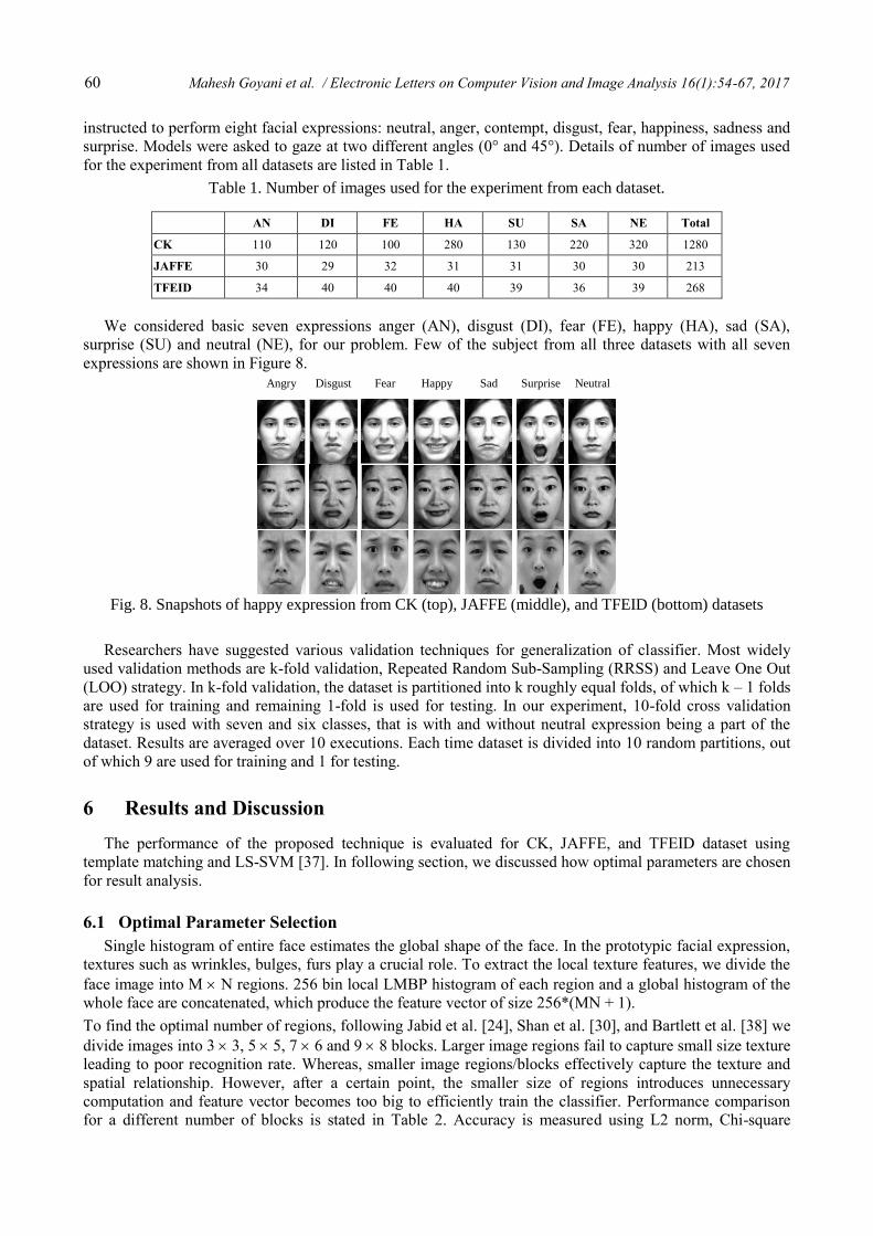
We considered basic seven expressions anger (AN), disgust (DI), fear (FE), happy (HA), sad (SA),
surprise (SU) and neutral (NE), for our problem. Few of the subject from all three datasets with all seven
expressions are shown in Figure 8.
Angry Disgust Fear Happy Sad Surprise Neutral
Fig. 8. Snapshots of happy expression from CK (top), JAFFE (middle), and TFEID (bottom) datasets
Researchers have suggested various validation techniques for generalization of classifier. Most widely
used validation methods are k-fold validation, Repeated Random Sub-Sampling (RRSS) and Leave One Out
(LOO) strategy. In k-fold validation, the dataset is partitioned into k roughly equal folds, of which k – 1 folds
are used for training and remaining 1-fold is used for testing. In our experiment, 10-fold cross validation
strategy is used with seven and six classes, that is with and without neutral expression being a part of the
dataset. Results are averaged over 10 executions. Each time dataset is divided into 10 random partitions, out
of which 9 are used for training and 1 for testing.
6 Results and Discussion
The performance of the proposed technique is evaluated for CK, JAFFE, and TFEID dataset using
template matching and LS-SVM [37]. In following section, we discussed how optimal parameters are chosen
for result analysis.
6.1 Optimal Parameter Selection
Single histogram of entire face estimates the global shape of the face. In the prototypic facial expression,
textures such as wrinkles, bulges, furs play a crucial role. To extract the local texture features, we divide the
face image into M N regions. 256 bin local LMBP histogram of each region and a global histogram of the
whole face are concatenated, which produce the feature vector of size 256*(MN + 1).
To find the optimal number of regions, following Jabid et al. [24], Shan et al. [30], and Bartlett et al. [38] we
divide images into 3 3, 5 5, 7 6 and 9 8 blocks. Larger image regions fail to capture small size texture
leading to poor recognition rate. Whereas, smaller image regions/blocks effectively capture the texture and
spatial relationship. However, after a certain point, the smaller size of regions introduces unnecessary
computation and feature vector becomes too big to efficiently train the classifier. Performance comparison
for a different number of blocks is stated in Table 2. Accuracy is measured using L2 norm, Chi-square
Mahesh Goyani et al. / Electronic Letters on Computer Vision and Image Analysis 16(1):54-67, 2017 61
measure and the proposed distance measure HNAD. The results show that HNAD has better discrimination
capacity compared to L2 norm and Chi-square distance. We chose a number of regions to be 5 5, as it
gives a proper balance between accuracy and standard deviation of results from its mean.
Table 2. Recognition rate for a different number of regions, Dataset: CK.
Accuracy for 7-class problem Accuracy for 6-class problem
#Blocks L2 Norm Chi - Square HNAD L2 Norm Chi - Square HNAD
3 3 95.3 2.7 95.5 2.4 96.1 2.6 98.2 1.9 98.1 2.1 98.0 2.2
5 5 94.1 2.1 94.5 2.1 95.8 1.8 98.3 1.3 98.3 1.3 98.4 1.4
7 6 95.2 1. 8 95.2 1.8 96.9 1.7 98.1 2.5 98.0 2.4 98.1 2.5
9 8 94.9 2.2 95.4 1.5 96.3 1.5 99.2 1.1 99.2 1.1 99.3 1.1
6.2 Performance Evaluation using Optimal Parameter Selection
From experimental results, we chose an optimal number of blocks to be 5 5. Using HNAD measure, we
achieved a recognition rate of 95.8% and 98.4% for a 7-class and 6-class problem respectively for CK
dataset. Similarly, the accuracy of 97.2% and 95.2% is reported on JAFFE for a 6-class and 7-class
problems. Comparison of proposed method with various local descriptors like Gabor [38], LBP [30] and
LDP [24] is shown in Table 3 for CK and JAFFE dataset. Results show the superiority of proposed method
with HNAD measure.
Table 3. Performance comparison on CK and JAFFE dataset using template matching.
CK JAFFE
Descriptor C = 6 C = 7 C = 6 C = 7
Gabor [38] 83.7 4.5 78.9 4.8 81.9 6.4 75.5 5.8
LBP [30] 84.5 5.2 79.1 4.6 83.7 6.7 77.2 7.6
LDP [24] 89.2 2.5 86.9 2.8 87.4 5.6 82.6 4.1
LMBP 98.4 1.4 95.8 1.8 95.2 2.2 97.2 1.7
In recent time, LS-SVM [37] has emerged as a first choice classifier for researchers. We also conduct
experiments using LS-SVM with different kernels. Block based approach produces a very big feature vector.
For M N blocks, LMBP produces the feature vector of size 256 * (MN + 1). Training the classifier for such
a big vector is very difficult and time-consuming. Huge feature vector often leads to over trained model. In
order to reduce the dimensions of the feature vector, we used principal component analysis. From
experiment, we chose first 70 eigenvectors with highest eigenvalue for the projection. Results of this
experiment for state of the art methods on CK dataset are compared in Table 4. With RBF kernel, we
achieved highest recognition rate among all compared methods.
Table 4. Performance comparison of different methods on CK dataset using support vector machine
Accuracy for 6-class problem Accuracy for 7-class problem
Technique Linear (%) Poly. (%) RBF (%) Linear (%) Poly. (%) RBF (%)
Gabor [38] 89.4 3.0 89.4 3.0 89.8 3.1 86.6 4.1 86.6 4.1 86.8 3.6
LBP [30] 91.5 3.1 91.5 3.1 92.6 2.9 88.1 3.8 88.1 3.8 88.9 3.5
LDP [24] 94.9 1.2 94.9 1.2 96.4 0.9 92.8 1.7 92.8 1.7 93.4 1.5
LMBP 92.1 2.9 98.9 1.7 99.3 1.4 86.6 2.8 97.8 1.5 98.2 1.0
A similar experiment is conducted on JAFFE dataset. Comparison of proposed method with existing
work on JAFFE dataset is presented in Table 5.

62 Mahesh Goyani et al. / Electronic Letters on Computer Vision and Image Analysis 16(1):54-67, 2017
Table 5. Performance comparison of different methods on JAFFE using support vector machine
Accuracy for 6-class problem Accuracy for 7-class problem
Technique Linear (%) Poly. (%) RBF (%) Linear (%) Poly. (%) RBF (%)
Gabor [38] 85.1 5.0 85.1 5.0 85.8 4.1 79.7 4.2 79.7 4.2 80.8 3.7
LBP [30] 86.7 4.1 86.7 4.1 87.5 5.1 80.7 5.5 80.7 5.5 81.9 5.2
LDP [24] 89.9 5.2 89.9 5.2 90.1 4.9 84.9 4.7 84.9 4.7 85.4 4.0
LMBP 87.8 2.2 91.2 2.1 92.3 2.5 81.7 3.2 80.6 2.2 88.3 1.4
TFEID dataset is not much explored by researchers. We test the robustness of our method on TFEID also,
and results are depicted in Table 6. As stated earlier, we chose 70 features after PCA projection. Optimal
number of blocks chosen for experiment are also same as earlier, i.e. 5 5.
Table 6. Performance of LMBP on TFEID
Template Matching Machine Learning
#Class L2 Norm Chi - Square HNAD Linear (%) Polynomial (%) RBF (%)
6 89.9 4.1 90.31 4.3 91.78 3.9 92.9 4.1 85.8 3.6 92.5 4.2
7 86.4 5.2 86.5 5.3 89.9 5.2 90.0 4.8 87.9 5.6 90.4 5.1
Results discussed so far were averaged over all six or seven expressions. To get a better idea about
recognition rate of individual expression, confusion matrix for CK, JAFFE, and TFEID are shown in Table
7. Results are reported using LS-SVM with RBF kernel.
Table 7. Confusion matrix for a 7-class problem for all three datasets, classifier: LS-SVM (RBF)
Confusion matrix for CK Confusion matrix for JAFFE Confusion matrix for TFEID
AN DI FE HA SA SU NE AN DI FE HA SA SU NE AN DI FE HA SA SU NE
AN 98.0 0.3 0.7 0.0 0.8 0.0 0.2 85.6 2.3 5.3 1.1 3.3 0.8 1.6 88.3 5.2 2.3 1.0 1.5 0.6 1.1
DI 0.6 97.4 0.8 0.1 0.9 0.0 0.2 4.6 84.4 4.8 0.7 3.1 0.5 1.9 4.5 87.2 3.6 1.4 1.1 0.9 1.3
FE 0.8 0.8 97.7 0.1 0.1 0.3 0.2 5.6 3.4 85.2 1.6 2.1 0.0 2.1 3.2 2.1 91.1 0.6 1.3 0.8 0.9
HA 0.1 0.1 0.1 99.6 0.1 0.0 0.0 2.1 1.2 1.1 93.2 0.7 0.3 1.4 1.4 1.1 2.9 92.1 0.4 1.1 1.0
SA 0.7 1.1 0.6 0.2 96.2 0.2 1.0 2.3 3.8 2.3 1.7 85.2 1.2 3.5 1.9 2.1 3.4 1.1 89.2 0.2 2.1
SU 0.0 0.1 0.1 0.0 0.0 99.8 0.0 0.9 1.7 2.3 1.1 0.7 93.2 0.1 1.2 0.7 2.1 0.8 0.1 94.2 0.9
NE 0.1 0.2 0.3 0.2 0.4 0.1 98.7 1.9 0.9 1.5 0.8 3.5 0.2 91.2 0.7 1.8 1.4 0.6 4.2 0.3 91.0
Avg. 98.2 88.3 90.4
For CK dataset, the average accuracy of 98.2% for seven classes is really encouraging, compared to
91.4% accuracy reported by Shan et al [30]. Bartlett et al. [38] obtained the highest recognition rate of 93.3%
using a subset of Gabor filters with Adaboost feature selection and SVM classifier. Using three layers neural
network, Tian [39] achieved 94% recognition rate with Gabor features along with geometric features. Results
of proposed method are compared with various existing approaches on CK dataset in Table 8.
Table 8. Reported accuracy of state of the art methods on CK dataset.
Literature #Subjects #Class Strategy Acc.(%)
Yang et al. [40] 96 6 - 92.3
Shan et al. [30] 96 6 10 Fold 92.1
Littlewort et al. [41] 90 7 - 93.3
Wenfei et al. [42] 94 7 10 Fold 91.5
Oyuang et al. [43] 94 6 - 93.5
Mahesh Goyani et al. / Electronic Letters on Computer Vision and Image Analysis 16(1):54-67, 2017 63
Literature #Subjects #Class Strategy Acc.(%)
Zheng et al. [44] 97 6 10-Fold 94.0
LMBP + HNAD 97 7 10-Fold 95.8
LMBP + HNAD 97 6 10-Fold 98.4
LMBP + SVM 97 7 10-Fold 98.2
LMBP + SVM 97 6 10-Fold 99.3
JAFFE dataset is another widely accepted facial expression dataset, developed by Lyons et al [25].
JAFFE does not have as much diversity as CK has. Subjects in JAFFE belong to the same ethnicity and all
are female. The highest recognition rate of 88.3% and 92.3% is achieved using SVM with RBF kernel for
seven and six class problem, respectively. Results of proposed method are compared with various state of the
art methods in Table 9 for JAFFE dataset.
Table 9. Reported accuracy of state of the art methods on JAFFE dataset.
Literature Method Acc. (%)
Lekshmi and Sasikumar [45] SVM 86.9
Zhi and Ruan [46] 2D-DLPP 95.9
Zhao, Zhuang, and Xu [47] PCA + ANN 93.7
Owusu et al. [48] Gabor + MFFNN 96.8
Proposed
LMBP + HNAD (C = 7) 97.2
LMBP + HNAD (C = 6) 95.2
LMBP + SVM (C = 7) 88.3
LMBP + SVM (C = 6) 92.3
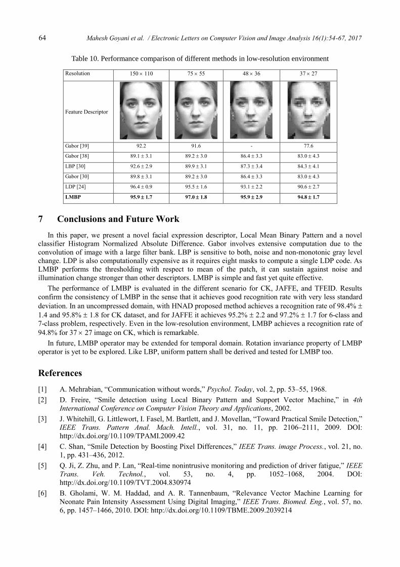
6.3 Expression Recognition in Low Resolution
It is not always possible to acquire high-quality images under all circumstances. In certain applications
such as home monitoring, surveillance applications, smart meeting, only low-resolution videos are available
[39]. Expression recognition in low resolution is an almost unaddressed area, very little work is done in this
field. In our experiment, we studied the performance of LMBP operator at four different resolutions: 150
110, 75 55, 48 36 and 37 27. Low-resolution images are derived by down-sampling the original
images. Shan et al. [30] conducted the experiment in low resolution with LBP and Gabor features derived by
convolving the image with 40 gabor filter banks. The classification was performed using SVM. Tian [39]
selected 375 image sequences from CK dataset. He used geometric and appearance features. Geometric
features were computed using feature tracking and feature selection. Appearance features were derived using
40 gabor filter banks. The three-layer neural network was used for expression classification. Due to down
sampling and smaller size of the image, geometric features do not make sense, as detecting and tracking
geometric feature is also difficult and vulnerable in such environment. So, only appearance features should
be considered for classification. Jabid et al. [24] derived LDP features using 8 Kirsch edge detectors. They
achieved notable recognition rate using SVM. In Table 10, the performance of LMBP in low resolution is
compared with various existing approaches.
64 Mahesh Goyani et al. / Electronic Letters on Computer Vision and Image Analysis 16(1):54-67, 2017
Table 10. Performance comparison of different methods in low-resolution environment
Resolution 150 110 75 55 48 36 37 27
Feature Descriptor
Gabor [39] 92.2 91.6 - 77.6
Gabor [38] 89.1 3.1 89.2 3.0 86.4 3.3 83.0 4.3
LBP [30] 92.6 2.9 89.9 3.1 87.3 3.4 84.3 4.1
Gabor [30] 89.8 3.1 89.2 3.0 86.4 3.3 83.0 4.3
LDP [24] 96.4 0.9 95.5 1.6 93.1 2.2 90.6 2.7
LMBP 95.9 1.7 97.0 1.8 95.9 2.9 94.8 1.7
7 Conclusions and Future Work
In this paper, we present a novel facial expression descriptor, Local Mean Binary Pattern and a novel
classifier Histogram Normalized Absolute Difference. Gabor involves extensive computation due to the
convolution of image with a large filter bank. LBP is sensitive to both, noise and non-monotonic gray level
change. LDP is also computationally expensive as it requires eight masks to compute a single LDP code. As
LMBP performs the thresholding with respect to mean of the patch, it can sustain against noise and
illumination change stronger than other descriptors. LMBP is simple and fast yet quite effective.
The performance of LMBP is evaluated in the different scenario for CK, JAFFE, and TFEID. Results
confirm the consistency of LMBP in the sense that it achieves good recognition rate with very less standard
deviation. In an uncompressed domain, with HNAD proposed method achieves a recognition rate of 98.4%
1.4 and 95.8% 1.8 for CK dataset, and for JAFFE it achieves 95.2% 2.2 and 97.2% 1.7 for 6-class and
7-class problem, respectively. Even in the low-resolution environment, LMBP achieves a recognition rate of
94.8% for 37 27 image on CK, which is remarkable.
In future, LMBP operator may be extended for temporal domain. Rotation invariance property of LMBP
operator is yet to be explored. Like LBP, uniform pattern shall be derived and tested for LMBP too.
References
[1] A. Mehrabian, “Communication without words,” Psychol. Today, vol. 2, pp. 53–55, 1968.
[2] D. Freire, “Smile detection using Local Binary Pattern and Support Vector Machine,” in 4th
International Conference on Computer Vision Theory and Applications, 2002.
[3] J. Whitehill, G. Littlewort, I. Fasel, M. Bartlett, and J. Movellan, “Toward Practical Smile Detection,”
IEEE Trans. Pattern Anal. Mach. Intell., vol. 31, no. 11, pp. 2106–2111, 2009. DOI:
http://dx.doi.org/10.1109/TPAMI.2009.42
[4] C. Shan, “Smile Detection by Boosting Pixel Differences,” IEEE Trans. image Process., vol. 21, no.
1, pp. 431–436, 2012.
[5] Q. Ji, Z. Zhu, and P. Lan, “Real-time nonintrusive monitoring and prediction of driver fatigue,” IEEE
Trans. Veh. Technol., vol. 53, no. 4, pp. 1052–1068, 2004. DOI:
http://dx.doi.org/10.1109/TVT.2004.830974
[6] B. Gholami, W. M. Haddad, and A. R. Tannenbaum, “Relevance Vector Machine Learning for
Neonate Pain Intensity Assessment Using Digital Imaging,” IEEE Trans. Biomed. Eng., vol. 57, no.
6, pp. 1457–1466, 2010. DOI: http://dx.doi.org/10.1109/TBME.2009.2039214
Mahesh Goyani et al. / Electronic Letters on Computer Vision and Image Analysis 16(1):54-67, 2017 65
[7] B. Fasel and J. Luettin, “Automatic facial expression analysis: A survey,” Pattern Recognit., vol. 36,
no. 1, pp. 259–275, 2003. DOI: http://dx.doi.org/10.1016/S0031-3203(02)00052-3
[8] Z. Zeng, M. Pantic, G. I. Roisman, and T. S. Huang, “A survey of affect recognition methods: Audio,
visual, and spontaneous expressions,” IEEE Trans. Pattern Anal. Mach. Intell., vol. 31, no. 1, pp. 39–
58, 2009. DOI: http://dx.doi.org/10.1109/TPAMI.2008.52
[9] M. Pantic and I. Patras, “Dynamics of facial expression: Recognition of facial actions and their
temporal segments from face profile image sequences,” IEEE Trans. Syst. Man, Cybern. Part B
Cybern., vol. 36, no. 2, pp. 433–449, 2006. DOI: http://dx.doi.org/10.1109/TSMCB.2005.859075
[10] T. R. Almaev and M. F. Valstar, “Local Gabor Binary Patterns from three orthogonal planes for
automatic facial expression recognition,” in Humaine Association Conference on Affective Computing
and Intelligent Interaction, 2013, pp. 356–361. DOI: http://dx.doi.org/10.1109/ACII.2013.65
[11] R. Highfield, R. Wiseman, and R. Jenkins, “How your looks betray personality,” New Scientists,
2009.
[12] C. Darvin, The Expression of the Emotions in Man and Animals. London: J. Murray, 1872.
[13] P. Ekman and W. V Friesen, “Constants across cultures in the face and emotion,” J. Pers. Soc.
Psychol., vol. 17, no. 2, pp. 124–129, 1971. DOI: http://dx.doi.org/10.1037/h0030377
[14] C. A. Corneanu, O. Marc, J. F. Cohn, and E. Sergio, “Survey on RGB, 3D, Thermal, and Multimodal
approaches for facial expression recognition: History, trends, and affect-related applications,” IEEE
Trans. Pattern Anal. Mach. Intell., vol. 38, no. 8, pp. 1548–1568, 2016. DOI:
http://dx.doi.org/10.1109/TPAMI.2016.2515606
[15] Y. Tian, T. Kanade, and J. F. Cohn, “Evaluation of Gabor-wavelet-based facial action unit
recognition in image sequences of increasing complexity,” in IEEE International Conference on
Automatic Face and Gesture Recognition, 2002, pp. 2–7.
[16] T. Ojala, P. Matti, and H. David, “A comparative study of texture measures with classification based
on featured distributions,” Pattern Recognit., vol. 29, no. 1, pp. 51–59, 1996. DOI:
http://dx.doi.org/10.1016/0031-3203(95)00067-4
[17] Y. Yacoob and L. S. Davis, “Recognizing human facial expressions from long image sequences using
Optical Flow,” IEEE Trans. Pattern Anal. Mach. Intell., vol. 18, no. 6, pp. 636–642, 1996. DOI:
http://dx.doi.org/10.1109/34.506414
[18] M. Rosenblum, Y. Yacoob, and L. S. Davis, “Human expression recognition from motion using a
radial basis function network architecture.,” IEEE Trans. Neural Networks, vol. 7, no. 5, pp. 1121–
1138, 1996. DOI: http://dx.doi.org/10.1109/72.536309
[19] M. A. Turk and A. P. Pentland, “Face recognition using eigenfaces,” Journal of Cognitive
Neuroscience, vol. 3, no. 1. pp. 72–86, 1991. DOI: http://dx.doi.org/10.1109/CVPR.1991.139758
[20] P. N. Belhumeur, J. P. Hespanha, and D. J. Kriegman, “Eigenfaces vs. Fisherfaces: Recognition using
class specific linear projection,” IEEE Trans. Pattern Anal. Mach. Intell., vol. 19, no. 7, pp. 711–720,
1997. DOI: http://dx.doi.org/10.1109/34.598228
[21] M. Bartlett and T. J. Sejnowski, “Independent components of face images: A representation for face
recognition,” in 4th Annual Joint Symposium on Neural Computation, 1997.
[22] T. Ojala, M. Pietikainen, and D. Harwood, “A comparative study of texture measures with
classification based on feature distributions,” Pattern Recognit., vol. 29, no. 1, pp. 51–59, 1996.
[23] T. Ojala, M. Pietikäinen, and T. Mäenpää, “A generalized local binary pattern operator for
multiresolution gray scale and rotation invariant texture classification,” in International Conference
on Advances in Pattern Recognition, 2001, pp. 399–408.
[24] T. Jabid, M. H. Kabir, and O. Chae, “Robust facial expression recognition based on local directional
pattern,” ETRI J., vol. 32, no. 5, pp. 784–794, 2010. DOI:
http://dx.doi.org/10.4218/etrij.10.1510.0132
[25] M. Lyons and S. Akamatsu, “Coding facial expressions with gabor wavelets,” in third IEEE
Conference on Automatic Face and Gesture Recognition, 1998, pp. 200–205. DOI:
http://dx.doi.org/10.1109/AFGR.1998.670949
66 Mahesh Goyani et al. / Electronic Letters on Computer Vision and Image Analysis 16(1):54-67, 2017
[26] A. Samal and P. A. Lyengar, “Automatic recognition and analysis of human faces and facial
expressions : A survey,” IEEE Trans. Pattern Recognit., vol. 25, no. 1, pp. 65–77, 1992.
[27] Y. L. Tian, T. Kanade, and J. F. Cohn, “Facial expression analysis,” Handb. Face Recognit., pp. 247–
275, 2005. DOI: http://dx.doi.org/10.1007/0-387-27257-7_12
[28] M. N. Dailey, C. Joyce, M. J. Lyons, M. Kamachi, H. Ishi, J. Gyoba, and G. W. Cottrell, “Evidence
and a computational explanation of cultural differences in facial expression recognition.,” Emotion,
vol. 10, no. 6, pp. 874–893, 2010. DOI: http://dx.doi.org/10.1037/a0020019
[29] M. Murtaza, M. Sharif, M. Raza, and J. H. Shah, “Analysis of Face Recognition under varying facial
expression: A survey,” Int. Arab J. Inf. Technol., vol. 10, no. 5, pp. 378–388, 2013.
[30] C. Shan, S. Gong, and P. W. Mcowan, “Facial expression recognition based on Local Binary
Patterns : A comprehensive study,” Image Vis. Comput., vol. 27, no. 6, pp. 803–816, 2009.
[31] T. Ojala, M. Pietikainen, and T. Maenpaa, “Multiresolution gray-scale and rotation invariant texture
classification with local binary patterns,” IEEE Trans. Pattern Anal. Mach. Intell., vol. 24, no. 7, pp.
971–987, 2002. DOI: http://dx.doi.org/10.1109/TPAMI.2002.1017623
[32] T. Senechal, V. Rapp, H. Salam, R. Seguier, K. Bailly, and L. Prevost, “Facial action recognition
combining heterogeneous features via multikernel learning,” IEEE Trans. Syst. Man Cybern. B
Cybern., vol. 42, no. 4, pp. 993–1005, 2012. DOI: http://dx.doi.org/10.1109/TSMCB.2012.2193567
[33] R. Hablani, N. Chaudhari, and S. Tanwani, “Recognition of facial expressions using Local Binary
Patterns of important facial parts,” Int. J. Image Process., vol. 7, no. 2, pp. 163–170, 2013.
[34] T. Kanade, J. F. Cohn, and Y. Tian, “Comprehensive database for facial expression analysis,” in 4th
IEEE International Conference on Automatic Face and Gesture Recognition, 2000, pp. 46–53. DOI:
http://dx.doi.org/10.1109/AFGR.2000.840611
[35] M. J. Lyons, “Automatic classification of single facial images,” IEEE Trans. Pattern Anal. Mach.
Intell., vol. 21, no. 12, pp. 1357–1362, 1999. DOI: http://dx.doi.org/10.1109/34.817413
[36] L.-F. Chen and Y.-S. Yen, “Taiwanese Facial Expression Image Database.” Brain Mapping
Laboratory, Institute of Brain Science, National Yang-Ming University, Taipei, Taiwan., 2007.
[37] J. A. K. Suykens, L. Lukas, P. Van Dooren, B. De Moor, and J. Vandewalle, “Least Squares Support
Vector Machine classifers: A large scale algorithm,” in European Conference on Circuit Theory and
Design, 1999, pp. 839–842.
[38] M. S. Bartlett, G. Littlewort, M. Frank, C. Lainscsek, I. Fasel, and J. Movellan, “Recognizing facial
expression: Machine learning and application to spontaneous behavior,” in IEEE Computer Society
Conference on Computer Vision and Pattern Recognition, 2005, vol. 2, pp. 568–573.
[39] Y. T. Y. Tian, “Evaluation of Face Resolution for Expression Analysis,” in 2004 Conference on
Computer Vision and Pattern Recognition Workshop, 2004, pp. 1–7.
[40] P. Yang, Q. Liu, and D. N. Metaxas, “Exploring facial expressions with compositional features,” in
IEEE Computer Society Conference on Computer Vision and Pattern Recognition, 2010, pp. 2638–
2644. DOI: http://dx.doi.org/10.1109/CVPR.2010.5539978
[41] G. Littlewort, M. S. Bartlett, I. Fasel, J. Susskind, and J. Movellan, “Dynamics of facial expression
extracted automatically from video,” Image Vis. Comput., vol. 24, no. 6, pp. 615–625, 2006. DOI:
http://dx.doi.org/10.1016/j.imavis.2005.09.011
[42] G. Wenfei, C. Xiang, Y. V. Venkatesh, D. Huang, and H. Lin, “Facial expression recognition using
radial encoding of local Gabor features and classifier synthesis,” Pattern Recognit., vol. 45, no. 1, pp.
80–91, 2012.
[43] Y. Ouyang, N. Sang, and R. Huang, “Robust automatic facial expression detection method based on
sparse representation plus LBP map,” Opt. - Int. J. Light Electron Opt., vol. 124, no. 24, pp. 6827–
6833, 2013. DOI: http://dx.doi.org/10.1016/j.ijleo.2013.05.076
[44] H. Zheng, X. Geng, D. Tao, and Z. Jin, “A Multi-Task Model for simultaneous face identification and
facial expression recognition,” Neurocomputing, vol. 171, pp. 515–523, 2016. DOI:
http://dx.doi.org/10.1016/j.neucom.2015.06.079

Mahesh Goyani et al. / Electronic Letters on Computer Vision and Image Analysis 16(1):54-67, 2017 67
[45] L. Praseeda and Sasikumar, “Analysis of facial expression using Gabor and SVM,” Int. J. Recent
Trends Eng., vol. 1, no. 2, pp. 47–50, 2009.
[46] R. Zhi and Q. Ruan, “Facial expression recognition based on Two-dimensional Discriminant Locality
Preserving Projections,” Neurocomputing, vol. 71, no. 7, pp. 1730–1734, 2008. DOI:
http://dx.doi.org/10.1016/j.neucom.2007.12.002
[47] L. Zhao, “Facial expression recognition based on PCA and NMF,” in 7th World Congress on
Intelligent Control and Automation, 2008, no. 4, pp. 6826–6829.
[48] E. Owusu, Y. Zhan, and Q. R. Mao, “A Neural-AdaBoost based facial expression recognition
system,” Expert Syst. Appl., vol. 41, no. 7, pp. 3383–3390, 2014. DOI:
http://dx.doi.org/10.1016/j.eswa.2013.11.041