Realtime Depth Estimation and Obstacle

Detection from Monocular Video

Andreas Wedel1,2, Uwe Franke1, Jens Klappstein1,Thomas Brox2, and Daniel Cremers2

1 DaimlerChrysler Research and Technology, REI/AI,71059 Sindelfingen, Germany

2 Computer Vision and Pattern Recognition Group,Rheinische Friedrich-Wilhelms Univeristat, 53117 Bonn, Germany

Abstract. This paper deals with the detection of arbitrary static ob-jects in traffic scenes from monocular video using structure from motion.A camera in a moving vehicle observes the road course ahead. The cameratranslation in depth is known. Many structure from motion algorithmswere proposed for detecting moving or nearby objects. However, detect-ing stationary distant obstacles in the focus of expansion remains quitechallenging due to very small subpixel motion between frames. In thiswork the scene depth is estimated from the scaling of supervised imageregions. We generate obstacle hypotheses from these depth estimates inimage space. A second step then performs testing of these by comparingwith the counter hypothesis of a free driveway. The approach can detectobstacles already at distances of 50m and more with a standard focallength. This early detection allows driver warning and safety precautionin good time.

1 Introduction

Automatic detection and verification of objects in images is a central challengein computer vision and pattern analysis research. An important application isrobustly hypothesizing and verifying obstacles for safety applications in intelli-gent vehicles. The practical value of such systems becomes evident as obstacle

Fig. 1. Six out of ten front–end crashes could be prevented if safety systems reacteda split second earlier than the driver. Detecting arbitrary obstacles from monocularvideo in the road course ahead, however, is quite challenging.

K. Franke et al. (Eds.): DAGM 2006, LNCS 4174, pp. 475–484, 2006.c© Springer-Verlag Berlin Heidelberg 2006

476 A. Wedel et al.

detection is a prerequisite to warn the driver of approaching hazards (see Fig. 1).Commonly used radar sensors lack detecting static objects therefore we tacklethis problem using computer vision.

For a camera mounted in a vehicle with a given camera translation in depth,detecting obstacles in traffic scenes has three major challenges:

1. The algorithm has to run in real time with minimum delay in reaction time.2. Obstacles have to be detected at large distances to route the vehicle or warn

the driver as early as possible.3. The position and horizontal dimension of an obstacle have to be estimated

precisely to safely guide the vehicle in case an emergency brake is insufficient.

The first two challenges demand an algorithm able to detect obstacles in thefocus of expansion where optical flow displacement vectors between consecutiveframes are extremely small. Overcoming this by skipping frames violates the firstconstraint. The last challenge requires robust verification of obstacle boundaries.

Traditional vision based obstacle detection relies on depth estimation fromstereo systems [7]. Such systems work well. However, single cameras are alreadyavailable in series production performing numerous vision based driver assis-tance algorithms such as intelligent headlight control and night view. Obstacledetection from a single camera is, hence, a desirable alternative.

According to [1,14] obstacle detection in monocular vision can be split intomethods employing a–priori knowledge and others based on the relative imagemotion. Former algorithms need to employ strict assumptions regarding the ap-pearance of observed objects. Since we are interested in a model free approach, wehave to use latter methods. Proposed realtime optical flow algorithms [3,11,13]and obstacle detection based on those [12] calculate the displacement betweenconsecutive frames of an image sequence. In such a basic approach, integratingflow vectors over successive image pairs is subject to drifts and therefore thesealgorithms are not suitable for the posed problem. Moreover, these methods de-tect obstacles in two steps firstly calculating flow vectors for every pixel andsecondly analyzing those flow vectors. Working directly in image space is moredesirable as all the information available is accessed directly.

We propose an obstacle detection algorithm in the two standard steps:

1. Hypothesis generation from estimating scene depth in image space.2. Candidate testing by analyzing perspective transformation over time.

In the first step, conclusions about scene depth are drawn from the scalingfactor of image regions, which is determined using region tracking. We use thetracking algorithm described in [8] which is consistent over multiple frames ofan image sequence and directly estimates scale and translation in image space.For an evaluation of different tracking algorithms we refer to [5]. If distancemeasurements fall below a given threshold, obstacle hypotheses are generated.Due to the restricted reliability of depth from region scaling, such an approachcan result in false hypotheses which have to be dismissed.

The testing of generated hypotheses is performed in the second step. We checkwhether the observed perspective distortion over time corresponds to an obstacle

Realtime Depth Estimation and Obstacle Detection from Monocular Video 477

with distance given from hypothesis generation or to a free driveway. In such anapproach we are able to detect arbitrary obstacles directly in image space. Thetwo steps will be investigated separately in Sects. 2 and 3. Experimental resultson real image data can be found in Sect. 4. A final conclusion and motivationfor further work will be given in Sect. 5.

2 Depth Tracking from Monocular Video

This section investigates the mathematical foundation for reconstructing scenedepth from monocular vision. First we describe the underlying perspective pro-jection and the model used for depth computation. Then we describe how depthinformation can be computed from scaling of image regions and how this factcan be used to efficiently detect stationary obstacles. Finally we investigate theerror in depth estimation.

We use a monocular camera mounted on a vehicle such that the camera’soptical axis e3 coincides with the vehicle translation direction. The referencesystem is the left–handed camera coordinate system (0, e1, e2, e3) with the e2

unit vector being the ground plane normal. In particular, we assume a flat groundand a straight road to travel on. The image plane has equation Z = f , where fis the focal length of the camera. The ground plane is Y = −Y0 with the cameraheight Y0. For a point X = (X, Y, Z)� in 3–D space we obtain the correspondingimage point x = (x, y)� by a perspective projection:

x =f

Z

(X−Y

). (1)

In practice the camera coordinate system e3 axis usually is not parallel to theground plane. Camera rotation can be compensated transforming the camera toa virtual forward looking camera in a similar way as described in [9]. The cameratranslation in depth between consecutive frames is known from inertial sensors.

Obstacles are assumed to be axis parallel bounded boxes. This states that theZ coordinate of the obstacle plane facing the camera is constant. In practice therelative depths on obstacle surfaces are small compared to the distance betweenobstacle and camera such that this assumption is a good approximation.

Let X(t) = (X(t), Y (t), Z(t))� be a point at time t and x(t) its projectedimage point. The camera translation in depth between time t and t+τ is T (t, τ)leading to X(t + τ) = X(t) + T (t, τ). The camera translational and rotationalvelocity is T (t) and Ω(t) respectively. Particular coordinates are represented bysubscripted characters. Traditional structure from motion algorithms based onoptical flow involve using the image velocity field mentioned by Longuet-Higginsand Prazdny in [10] (the time argument is dropped due to better readability):

x =1Z

(xTZ − fTX

yTZ − fTX

)−

⎛⎝ ΩX

xyf + ΩY

(f + x2

f

)+ ΩZy

ΩX

(f + y2

f

)+ ΩY

xyf + ΩZx

⎞⎠ . (2)

478 A. Wedel et al.

Such algorithms are exact for time instances where image velocities are measur-able. However, flow vectors measure the displacement of image points betweenframes. Therefore resolving (2) using an explicit or implicit integration methodinduces drifts by adding up errors in inter–frame motions. We divide the motionof image regions into two parts and show that under the given conditions thescene depth can be estimated solely by estimating the scaling factor of imageregions. The transformation of an image point for a pure translation using (1)becomes

x(t + τ) =f

Z(t + τ)

(X(t + τ)Y (t + τ)

)=

f

Z(t) + TZ(t, τ)

(X(t) + TX(t, τ)Y (t) + TY (t, τ)

)(3)

=Z(t)

Z(t) + TZ(t, τ)︸ ︷︷ ︸s(t,τ)

f

Z(t)

(X(t)Y (t)

)︸ ︷︷ ︸

x(t)

+f

Z(t) + TZ(t, τ)

(TX(t, τ)TY (t, τ)

). (4)

It should be pointed out, that we use absolute image coordinates and notvelocities for computation. With a correctly given vehicle translation and dis-placement of image points, scene depth can be directly calculated over large timescales. As only the translation in depth TZ(t, τ) is known, a single observation isnot sufficient to determine scene depth. With the assumed model though, frontfaces of obstacles have equal Z coordinates and therefore multiple observationsin an image region can be used to solve an over–determined equation system forthe scaling factor and the translation.

The key for depth reconstruction is to use the scale s(t, τ) directly obtainedby the used region tracking over multiple frames to calculate scene depth:

d ≡ Z(t) =s(t, τ)

1 − s(t, τ)TZ(t, τ) . (5)

Distance histogram. For reconstructing scene depth we observe the imageregion to which obstacles in 30m distance with 0.9m height are mapped (com-pare Fig. 4). This region is divided up into n overlapping image regions {Ri}n

i=0,which are individually tracked until their correlation coefficient surpasses a fixedthreshold. The estimated distances of the tracked regions are projected onto thex–axis in image space (which can be regarded as a discrete resolution of theviewing angle) to receive a distance histogram. Projected obstacle distances areweighted by distance from region center. An appropriate weighting function isthe triangular hat function ΔRi defined on the region width. With the imageregion distance d(Ri) and the characteristic function χRi(x) = 1 ⇔ x ∈ R thisresults in the following distance histogram (see Fig. 5):

d(x) =1∑

i χRi(x)ΔRi (x)

∑i

χRi(x)ΔRi(x)d(Ri) . (6)

Realtime Depth Estimation and Obstacle Detection from Monocular Video 479

Error in depth estimation. In this paragraph we will show how depthvariance can be calculated by error propagation taking into account errors dueto rotation as well. In real case scenarios rotational effects occur as steer angle,shocks and vibrations experienced by the vehicle can introduce rapid and largetransients in image space.

Recalling that (2) involves velocities, we use explicit Euler integration formodeling the incremental rotational transformation. For the analysis of rota-tional errors the translational part can be set to zero leading to:

x(t + τ) = x(t) + τ

⎛⎝ ΩX(t)x(t)y(t)

f + ΩY (t)(f + x(t)2

f

)+ ΩZ(t)y(t)

ΩX(t)(f + y(t)2

f

)+ ΩY (t)x(t)y(t)

f + ΩZ(t)x(t)

⎞⎠ . (7)

The constant terms in (7) will influence only the translation estimation andtherefore keep the scaling factor unchanged. The influence of the roll rate (ΩZ)when looking at each image coordinate equation by itself is constant, too. Theyaw rate (ΩY ) and pitch rate (ΩX) are linear and quadratic in the image coor-dinates and therefore will influence the scale factor. Let s be the estimated scalefactor, es the error in scale estimation, and s the true scale with zero rotation.From (7) it follows that

s = s + es + cx + cy . (8)

However, assuming the yaw and pitch angle to be bounded by ±10◦ and thefocal length to be greater than 800px leads to

c ≡ τΩ

f∈ [−2.2 · 10−4, 2.2 · 10−4

]. (9)

The limited image size (of 640 × 480 pixel) and the bounded values of the ro-tation parameters therefore limit the effect on estimation of region scale. Withknown scale variance from tracking σ2

s and variance in translation σ2TZ

the depthvariance can be calculated by error propagation from (5) and (8) via:

σ2d =

1(1 − s)2

TZ (σs + xσc + yσc)2 +s

1 − sσ2

TZ. (10)

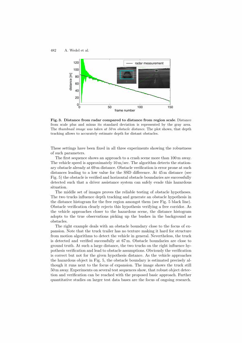
It has to be pointed out that the relative error in scale estimation becomessmaller as the scale factor increases, such that the influence of rotation on thescaling factor becomes negligible over large time scales (see Fig. 3).

The next section deals with obstacle detection based on the distance histogramfrom (6). The separation between depth estimation and obstacle detection allowsfor usage of distance histograms generated by alternative sensors (e.g. a scanningradar) for a sensor–fusion. Results obtained from depth estimation can be foundin Sect. 4.

480 A. Wedel et al.

3 Obstacle Detection by Hypothesis Verification

The distance histogram from the previous section can serve to find potential ob-stacles. If any entry in the image distance histogram falls below a fixed distancethreshold, an obstacle hypothesis is created. As pointed out in [6], robust com-puter vision algorithms should provide not only parameter estimates but alsoquantify their accuracy. Although we get the distance accuracy of an obstaclehypothesis by error propagation from tracking, this does not evaluate the prob-ability of an obstacle’s pure existence. This section describes obstacle detectionby hypothesis testing resulting in a quality specified output.

Let d be the distance of an obstacle hypothesis drawn from the distancehistogram. With the known camera translation in depth TZ the transformationof the obstacle in image space using (5) is

x′ = V (x) =(

d−TZ

d 00 d−TZ

d

)x . (11)

The counter hypothesis of a free driveway with plane equation e2 = −Y0 willbe transformed in image space using homogeneous coordinates according to

x′ = Q(x) =

⎡⎣1 0 0

0 1 00 TZ

Y01

⎤⎦x . (12)

Obviously this is only true for the ground plane up to the projected horizon.The hypothesis no obstacle above the horizon is set to be the identity (as thisis equivalent with obstacles being infinitely distant).

Hypothesis testing. Let F (x) and G(x) be the intensity value for the initialimage and the image after vehicle translation respectively. We assume a Gaussiandistribution of the intensity values and fixed standard deviation, thus for animage transformation function f corresponding to an image region R we get

pR(f) ∝ e−|G−F |2 (13)

with |G − F |2 being the sum of squared differences defined as

− log(pR(f)) =∑x∈R

(G(x′) − F (x))2 . (14)

p is maximal if the intensity value differences are minimal and vice versa. Thescope of hypotheses verification is finding the transformation with higher prob-ability. Let p1 = pR(V ) and p2 = pR(Q), it then follows

p1 > p2 ⇔ log p1 > log p2 ⇔ log p1 − log p2 > 0 . (15)

Therefore hypothesis testing boils down to calculating the SSD–difference forthe two transformation assumptions. The absolute distance from zero representsthe reliability of the result.

Realtime Depth Estimation and Obstacle Detection from Monocular Video 481

−300 −200 −100 0 100 200 300

−50

0

50

0.5m translation

−300 −200 −100 0 100 200 300

−50

0

50

2m translation

0

0.5

1

Fig. 2. Difference between flow field from planar ground (no flow above horizon) andobstacle in 30m distance (planar motion parallax) for different camera translation indepth. The brightness corresponds to the length of the flow difference vector. Clearly,the challenge to distinguish between an obstacle and the planar ground near the focusof expansion by relative image motion becomes visible (camera focal length 689 pixel).

In practice, vehicle translation is not solely restricted to translation in TZ .However, the motion parameters not included in the model can be compensatedfor the most part by estimating an extra region shift. Nevertheless, over largertime scales, hypothesis verification becomes more and more prone to errors dueto lighting changes and the unmodelled motion.

Therefore, in the verification case, we restrict ourselves to time scales of20 frames (in practice this corresponds to camera translations of more than 2m).As indicated in Fig. 2 and by our experimental results, such a translation pro-vides a sufficient difference between the two transformation assumptions andallows for reliable hypothesis testing.

4 Experimental Results

The proposed algorithm has been tested on real roads. The results are given inthe following.

Comparison with distance from radar. A textured wall with a cornerreflector behind the wall represents the obstacle. Due to the breadboard con-struction the distance measurement from radar is taken as the reference valueand compared to distance from depth tracking. The results in Fig. 3 show, thatdistance measurement by scale is error-prune around the initial frame. This isnot surprising as the scale factor is close to 1 and therefore division by 1 − s in(5) for distance computation leads to high inaccuracies. However, distance com-putation becomes quickly stable with greater vehicle translation. This clearlyshows that distance estimation over large time scales is indispensable.

Obstacle detection performance. In the remaining part of this section weshow three exemplary sequences from our test series on real roads to demonstratehypotheses generation and testing. Figure 4 shows the first frame for each of thesesequences. Notice that obstacle edges are present close to the focus of expansionwhat makes detection quite challenging.

The sequences are taken from a camera with 8.4mm focal length (8.4mmcorresponds to 840pixel) and 1.1m camera height. The correlation threshold forreplacing a depth tracker is set to 0.8. The threshold for hypothesis verificationin the distance histogram is set to 70m and restricted to the driving corridor.

482 A. Wedel et al.

0 50 100 1500

20

40

60

80

100

120

frame number

dist

ance

[m]

radar measurement

Fig. 3. Distance from radar compared to distance from region scale. Distancefrom scale plus and minus its standard deviation is represented by the gray area.The thumbnail image was taken at 50m obstacle distance. The plot shows, that depthtracking allows to accurately estimate depth for distant obstacles.

These settings have been fixed in all three experiments showing the robustnessof such parameters.

The first sequence shows an approach to a crash scene more than 100m away.The vehicle speed is approximately 10m/sec. The algorithm detects the station-ary obstacle already at 69m distance. Obstacle verification is error prone at suchdistances leading to a low value for the SSD difference. At 45m distance (seeFig. 5) the obstacle is verified and horizontal obstacle boundaries are successfullydetected such that a driver assistance system can safely evade this hazardoussituation.

The middle set of images proves the reliable testing of obstacle hypotheses.The two trucks influence depth tracking and generate an obstacle hypothesis inthe distance histogram for the free region amongst them (see Fig. 5 black line).Obstacle verification clearly rejects this hypothesis verifying a free corridor. Asthe vehicle approaches closer to the hazardous scene, the distance histogramadopts to the true observations picking up the bushes in the background asobstacles.

The right example deals with an obstacle boundary close to the focus of ex-pansion. Note that the truck trailer has no texture making it hard for structurefrom motion algorithms to detect the vehicle in general. Nevertheless, the truckis detected and verified successfully at 67m. Obstacle boundaries are close toground truth. At such a large distance, the two trucks on the right influence hy-pothesis verification and lead to obstacle assumptions. Obviously the verificationis correct but not for the given hypothesis distance. As the vehicle approachesthe hazardous object in Fig. 5, the obstacle boundary is estimated precisely al-though it runs next to the focus of expansion. The image shows the truck still50m away. Experiments on several test sequences show, that robust object detec-tion and verification can be reached with the proposed basic approach. Furtherquantitative studies on larger test data bases are the focus of ongoing research.

Realtime Depth Estimation and Obstacle Detection from Monocular Video 483

Fig. 4. Initial frames. The white box indicates the cropped image size shown inFig. 5. The black box marks the area used for depth tracking.

0

50

100

200

Fig. 5. Obstacle detection with distance histogram (black, scale on the left) andhypotheses verification (white, logarithmic scale, obstacle verified if above dashedline). The images show, that robust obstacle detection and verification is reached.

5 Conclusions

We have presented an algorithm for static obstacle detection in monocular imagesequences. The scene depth is estimated by the change of region scale in imagespace; obstacle hypotheses are generated if depth estimation falls below a fixedthreshold. To verify these hypotheses we check whether the observed transfor-mation in image space is more likely to be generated by a static object or by theflat ground.

We implemented the algorithm on a Pentium IV with 3.2GHz and achieveda framerate of 23 frames per second for the distance histogram calculation. Thedistance histogram and verification computation together run at approximately13 frames per second. To the authors’ knowledge, this is the fastest monocularmotion–base obstacle detection algorithm in literature for obstacles close to thefocus of expansion. The approach is easily applicable to other motion baseddistance measurements for obstacle detection and verification.

Further research will concentrate on speed gain. A wide range of algorithmsin literature was proposed to speed up and stabilize tracking in image space. Toname one possibility, pixel selection can be used to reduce computation time inregion tracking. It is in the focus of ongoing studies to intelligently distributethe single regions used for depth tracking in image space. Although the de-scribed system works well in unknown environments we believe that optimizingthe distribution and number of the tracked regions with respect to the cur-rently observed scene will lead to even better results and less computation time.Moreover, we will investigate means to improve obstacle detection by method

484 A. Wedel et al.

of segmentation [4] and globally optimized optic flow estimation [2] forced intodistinction of vertical and horizontal planes.

It also remains an open problem to detect moving obstacles in a monocularscenario. However, to pick up the threads given in the introduction, movingobjects are well detected by common radar sensors therefore a sensor fusioncombining measurements from an active radar and passive visual sensor is apromising field for further research.

References

1. M. Bertozzi, A. Broggi, M. Cellario, A. Fascioli, P. Lombardi, and M. Porta. Artifi-cial vision in road vehicles. In Proceedings of the IEEE, volume 90, pages 1258–1271,2002.

2. T. Brox, A. Bruhn, N. Papenberg, and J. Weickert. High accuracy optical flowestimation based on a theory for warping. In T. Pajdla and J. Matas, editors,Proc. 8th European Conference on Computer Vision, volume 3024 of LNCS, pages25–36. Springer, May 2004.

3. A. Bruhn, J. Weickert, and C. Schnorr. Lucas/Kanade meets Horn/Schunck: Com-bining local and global optic flow methods. International Journal of ComputerVision, 63(3):211–231, 2005.

4. D. Cremers and S. Soatto. Motion competition: A variational framework for piece-wise parametric motion segmentation. International Journal of Computer Vision,62(3):249–265, May 2005.

5. B. Deutsch, C. Graßl, F. Bajramovic, and J. Denzler. A comparative evaluationof template and histogram based 2D tracking algorithms. In DAGM-Symposium2005, pages 269–276, 2005.

6. W. Forstner. 10 pros and cons against performance characterization of visionalgorithms. Performance Characteristics of Vision Algorithms, 1996.

7. U. Franke and A. Joos. Real-time stereo vision for urban traffic scene understand-ing. In Proc. IEEE Conference on Intelligent Vehicles, pages 273–278, 2000.

8. G. Hager and P. Belhumeur. Efficient region tracking with parametric models ofgeometry and illumination. IEEE Transactions on Pattern Analysis and MachineIntelligence, pages 1025–1039, 1998.

9. Q. Ke and T. Kanade. Transforming camera geometry to a virtual downward-looking camera: Robust ego-motion estimation and ground-layer detection. InProc. IEEE Conference on Computer Vision and Pattern Recognition, pages 390–397, 2003.

10. H. Longuet-Higgins and K. Prazdny. The interpretation of a moving retinal image.In Proceedings of the Royal Society of London, volume 208 of Series B, BiologicalSciences, pages 385–397, July 1980.

11. B. Lucas and T. Kanade. An iterative image registration technique with an appli-cation to stereo vision. In Proceedings of the 7th International Joint Conferenceon Artificial Intelligence, pages 674–679, 1981.

12. C. Rabe, C. Volmer, and U. Franke. Kalman filter based detection of obstacles andlane boundary. In Autonome Mobile Systeme, volume 19, pages 51–58, 2005.

13. F. Stein. Efficient computation of optical flow using the census transform. InDAGM04, pages 79–86, 2004.

14. Z. Sun, G. Bebis, and R. Miller. On-road vehicle detection using optical sensors: Areview. In IEEE International Conference on Intelligent Transportation Systems,volume 6, pages 125 – 137, 2004.