real-time communication over cluster-tree wireless … · programming (ilp), where a grouping of...
TRANSCRIPT
Department of Control EngineeringFaculty of Electrical Engineering
Czech Technical University in PragueCzech Republic
in collaboration with
CISTER-ISEP Research UnitPolytechnic Institute of Porto
Portugal
Real-time Communicationover Cluster-tree Wireless
Sensor Networks
a doctoral thesis submitted in partial fulfilment ofthe requirements for the degree of
Doctor of Philosophy (Ph.D.)
by
Petr Jurcık
Prague, January 2010
Ph.D. Programme: Electrical Engineering and Information TechnologyBranch of study: Control Engineering and Robotics
Supervisor: Doc. Dr. Ing. Zdenek HanzalekCo-supervisor: Anis Koubaa, Ph.D.

c©Copyright byPetr Jurcık
All rights reservedJanuary 2010

To me and my family.

Acknowledgements
First of all, I would like to express my thanks to my thesis supervisor,Zdenek Hanzalek, and thesis co-supervisors, Anis Koubaa and Mario Alves,for their patient supervision, help and support leading towards this thesis. Iam also grateful to Eduardo Tovar, Ricardo Severino and all other people,that I met during my stay at CISTER-ISEP Research Unit in Porto, for theopportunity to be part of their group, for their help and especially for creatingan excellent working environment. Finally, I wish to express my appreciationfor numerous conference and journal reviewers provided me with many usefulcomments and valuable feedbacks on all submitted papers. Last, but notleast, acknowledgements belong to my family, friends and Radoff.
This work was carried out in collaboration with CISTER-ISEP ResearchUnit, and it was funded by FCT under the CISTER Research Unit (FCTUI 608), by the PLURALITY project (CONCREEQ/900/2001), by theARTIST2 NoE and by the Ministry of Industry and Trade of the CzechRepublic under the project 61 03001.
Czech Technical University in Prague Petr JurcıkJanuary 2010

Abstract
Modelling and simulation of the fundamental performance limits of WirelessSensor Networks (WSNs) is of paramount importance to understand theirbehaviour under the worst-case conditions and to make the appropriatedesign choices. This is particular relevant for time-sensitive WSN appli-cations, where the timing behaviour of the network protocols impacts onthe correct operation of these applications. Furthermore, energy efficiencyis a key requirement to be fulfilled in these applications since the wirelessnodes are usually battery-powered. In that direction this thesis contributeswith an accurate simulation model of the IEEE 802.15.4/ZigBee protocolsand an analytical methodology for the worst-case analysis and dimensioningof a static or even dynamically changing cluster-tree WSN where the datasink can either be static or mobile. The thesis is focused on the studyof WSNs with cluster-tree topology because it supports predictable andenergy efficient behaviour, which is suited for time-sensitive applicationsusing battery-powered nodes. On the other side, in contrast with the starand mesh topologies, the cluster-tree topology expresses several challengingand open research issues such as a precise cluster scheduling to avoid inter-cluster collisions (messages/beacons transmitted from nodes in differentoverlapping clusters). Hence, the next objective is to find the collision-freeperiodic schedule of clusters’ active portions, called Time Division ClusterSchedule (TDCS), while minimizing the energy consumption of the nodes andmeeting all data flows’ parameters. The thesis also shows how to apply theproposed methodologies to the specific case of IEEE 802.15.4/ZigBee beacon-enabled cluster-tree WSNs, as an illustrative example that confirms theapplicability of general approach for specific protocols. Finally, the validityand accuracy of the simulation model and methodologies are demonstratedthrough the comprehensive experimental and simulation studies. Using theproposed analytical methodologies and simulation model, system designersare able to easily configure the IEEE 802.15.4/ZigBee cluster-tree WSN for agiven application-specific Quality of Service (QoS) requirements prior to thenetwork deployment.
Keywords: cluster-tree; energy efficiency; IEEE 802.15.4; Network Calcu-lus; quality of service; real-time; simulation; wireless sensor network; ZigBee.

Goals and objectivesThe main goals of this work have been set as follows.
1. The design, implementation and evaluation of an accurate simulationmodel for IEEE 802.15.4 and ZigBee protocols focusing on the Guaran-teed Time Slot (GTS) mechanism and ZigBee hierarchical routing strat-egy in beacon-enabled cluster-tree Wireless Sensor Networks (WSNs).
2. The formulation, implementation and evaluation of a methodologythat solves the energy efficient clusters’ scheduling problem in a staticcluster-tree WSN with a predefined set of time-bounded data flows,assuming bounded communication errors.
3. The analysis of the interdependence among the reliability of datatransmission, the energy consumption of the nodes and the timelinessin IEEE 802.15.4/ZigBee beacon-enabled cluster-tree WSNs.
4. The formulation, implementation and evaluation of a methodology thatenables quick and efficient worst-case dimensioning of network resourcesin a static or even dynamically changing cluster-tree WSN where astatic or mobile sink gathers data from all sensor nodes, assumingbounded communication errors.
Contents
1 Introduction 11.1 Outline and Contribution . . . . . . . . . . . . . . . . . . . . 3
2 Overview of IEEE 802.15.4 and ZigBee 72.1 Introduction . . . . . . . . . . . . . . . . . . . . . . . . . . . . 72.2 Physical layer . . . . . . . . . . . . . . . . . . . . . . . . . . . 82.3 Data link layer . . . . . . . . . . . . . . . . . . . . . . . . . . 92.4 ZigBee network layer . . . . . . . . . . . . . . . . . . . . . . . 12
3 IEEE 802.15.4/ZigBee simulation model 173.1 Introduction . . . . . . . . . . . . . . . . . . . . . . . . . . . . 173.2 Related work . . . . . . . . . . . . . . . . . . . . . . . . . . . 183.3 Simulation model . . . . . . . . . . . . . . . . . . . . . . . . . 20
3.3.1 Simulation model structure . . . . . . . . . . . . . . . 203.3.2 User-defined attributes . . . . . . . . . . . . . . . . . . 22
3.4 Simulation setup . . . . . . . . . . . . . . . . . . . . . . . . . 243.4.1 Simulation vs. analytical models . . . . . . . . . . . . 24
3.5 Performance evaluation . . . . . . . . . . . . . . . . . . . . . 253.5.1 Impact of SO on the GTS throughput . . . . . . . . . 253.5.2 Impact of SO on the media access delay . . . . . . . . 31
3.6 Conclusions . . . . . . . . . . . . . . . . . . . . . . . . . . . . 35
4 Energy efficient scheduling for cluster-tree WSNs 374.1 Introduction . . . . . . . . . . . . . . . . . . . . . . . . . . . . 374.2 Related work . . . . . . . . . . . . . . . . . . . . . . . . . . . 394.3 System model . . . . . . . . . . . . . . . . . . . . . . . . . . . 41
4.3.1 Cluster-tree topology model . . . . . . . . . . . . . . . 414.3.2 Data flow model . . . . . . . . . . . . . . . . . . . . . 444.3.3 Cyclic nature . . . . . . . . . . . . . . . . . . . . . . . 454.3.4 Collision domains . . . . . . . . . . . . . . . . . . . . . 47
vii
viii CONTENTS
4.4 Time Division Cluster Scheduling . . . . . . . . . . . . . . . . 484.4.1 Duration of the cluster’s active portion . . . . . . . . 494.4.2 TDCS formulated as a cyclic extension of RCPS/TC . 514.4.3 Graph of the communication tasks . . . . . . . . . . . 544.4.4 Solution of the scheduling problem by ILP algorithm . 56
4.5 Time complexity . . . . . . . . . . . . . . . . . . . . . . . . . 584.6 Simulation study . . . . . . . . . . . . . . . . . . . . . . . . . 61
4.6.1 Simulation setup . . . . . . . . . . . . . . . . . . . . . 614.6.2 Simulation results . . . . . . . . . . . . . . . . . . . . 63
4.7 Conclusions . . . . . . . . . . . . . . . . . . . . . . . . . . . . 654.A Table of symbols . . . . . . . . . . . . . . . . . . . . . . . . . 68
5 Dimensioning and worst-case analysis of cluster-tree WSNs 695.1 Introduction . . . . . . . . . . . . . . . . . . . . . . . . . . . . 695.2 Related work . . . . . . . . . . . . . . . . . . . . . . . . . . . 715.3 Background on Network Calculus . . . . . . . . . . . . . . . . 745.4 System model . . . . . . . . . . . . . . . . . . . . . . . . . . . 79
5.4.1 Cluster-tree topology model . . . . . . . . . . . . . . . 795.4.2 Data flow model . . . . . . . . . . . . . . . . . . . . . 805.4.3 Time Division Cluster Schedule . . . . . . . . . . . . . 83
5.5 Data flow analysis . . . . . . . . . . . . . . . . . . . . . . . . 855.5.1 Upstream direction . . . . . . . . . . . . . . . . . . . . 855.5.2 Downstream direction . . . . . . . . . . . . . . . . . . 88
5.6 Worst-case network dimensioning . . . . . . . . . . . . . . . . 925.6.1 Per-router resources analysis . . . . . . . . . . . . . . 925.6.2 End-to-end delay analysis . . . . . . . . . . . . . . . . 95
5.7 Application to IEEE 802.15.4/ZigBee . . . . . . . . . . . . . . 985.7.1 Guaranteed bandwidth of a GTS . . . . . . . . . . . . 985.7.2 Characterization of the service curve . . . . . . . . . . 1005.7.3 IEEE 802.15.4/ZigBee cluster-tree WSN setup . . . . 102
5.8 Performance evaluation . . . . . . . . . . . . . . . . . . . . . 1045.8.1 Network setup . . . . . . . . . . . . . . . . . . . . . . 1055.8.2 Analytical evaluation . . . . . . . . . . . . . . . . . . . 1075.8.3 Experimental evaluation . . . . . . . . . . . . . . . . . 110
5.9 Discussion on mobility support . . . . . . . . . . . . . . . . . 1165.9.1 Adapting the logical topology . . . . . . . . . . . . . . 1165.9.2 Routing protocol . . . . . . . . . . . . . . . . . . . . . 117
5.10 Conclusions . . . . . . . . . . . . . . . . . . . . . . . . . . . . 1205.A Table of symbols . . . . . . . . . . . . . . . . . . . . . . . . . 121
6 Conclusions 123

Contents ix
Bibliography 132
Index 134
Curriculum vitae 134
Author’s publications 135

x Contents
List of Figures
2.1 Structure of the IEEE 802.15.4/ZigBee frames. . . . . . . . . 92.2 Superframe structure of IEEE 802.15.4. . . . . . . . . . . . . 102.3 The Inter-Frame Spacing. . . . . . . . . . . . . . . . . . . . . 122.4 IEEE 802.15.4/ZigBee network topologies. . . . . . . . . . . . 13
3.1 The structure of the simulation model. . . . . . . . . . . . . . 213.2 The user-defined attributes of the GTS mechanism. . . . . . . 233.3 The utilization of the GTS bandwidth. . . . . . . . . . . . . . 263.4 GTS throughput as a function of the rate. . . . . . . . . . . . 273.5 GTS throughput: simulation vs. analytical model. . . . . . . 283.6 GTS throughput as a function of the buffer capacity. . . . . . 293.7 GTS throughput: simulation vs. analytical model. . . . . . . 303.8 The media access delay as a function of the arrival data rate. 323.9 The media access delay as a function of the buffer capacity. . 333.10 Average vs. maximum media access delay. . . . . . . . . . . . 343.11 Delay of the frames stored in the FIFO buffer. . . . . . . . . 353.12 The media access delay: simulation vs. analytical model. . . . 36
4.1 Cluster-tree topology with 2 time-bounded data flows. . . . . 424.2 Timing among clusters 1,2 and 6 from Figure 4.1. . . . . . . . 434.3 Schedules for data flows in Figure 4.1. . . . . . . . . . . . . . 464.4 The carrier-sense area and collision domain. . . . . . . . . . . 474.5 In-trees of dummy-tasks relating to the data flows. . . . . . . 534.6 Graph G of the tasks corresponding to example in Figure 4.1. 554.7 ILP formulation for cyclic extension of the scheduling problem. 564.8 Gantt chart of TDCS including flows 1 and 2. . . . . . . . . . 574.9 Time line of TDCS corresponding to the example in Figure 4.1. 594.10 The simulation scenario in Opnet Modeler. . . . . . . . . . . 624.11 Reliability and sum of energy consumption. . . . . . . . . . . 634.12 E2e delay and energy consumption as a function of BO. . . . 64
xi
xii List of Figures
4.13 E2e delay as a function of macMaxFrameRetries. . . . . . . 654.14 E2e delay as a function of macMaxFrameRetries. . . . . . . 66
5.1 The basic system model in Network Calculus. . . . . . . . . . 745.2 Example of a cumulative input and output functions. . . . . . 755.3 The worst-case cluster-tree topology model. . . . . . . . . . . 815.4 General data flow model. . . . . . . . . . . . . . . . . . . . . 825.5 The queuing system model for the upstream direction. . . . . 865.6 The queuing system model for downstream direction. . . . . . 895.7 The locations of a sink router and correspondent data flows. . 925.8 Downstream bandwidth increase factor. . . . . . . . . . . . . 945.9 The worst-case service latencies. . . . . . . . . . . . . . . . . 1015.10 The test-bed deployment and sensory data traffic. . . . . . . 1055.11 The GUI of the Matlab analytical model. . . . . . . . . . . . 1065.12 The worst-case delay and bandwidth. . . . . . . . . . . . . . . 1085.13 The worst-case delay and buffer requirement. . . . . . . . . . 1095.14 The worst-case buffer requirement. . . . . . . . . . . . . . . . 1115.15 Theoretical vs. experimental data traffic. . . . . . . . . . . . 1125.16 The theoretical vs. experimental delay bounds. . . . . . . . . 1145.17 The worst-case and maximum end-to-end delays. . . . . . . . 1155.18 Two approaches to mobile sink behaviour. . . . . . . . . . . . 1175.19 The route update algorithm. . . . . . . . . . . . . . . . . . . 119
List of Tables
2.1 Star vs. mesh vs. cluster-tree topologies. . . . . . . . . . . . . 15
3.1 Relation between data rate and Packet Interarrival Time. . . 27
4.1 The user-defined parameters of the data flows from Figure 4.1. 444.2 Guaranteed bandwidth of clusters’ superframes. . . . . . . . . 514.3 Time complexity of TDCS algorithm. . . . . . . . . . . . . . 604.4 The user-defined parameters. . . . . . . . . . . . . . . . . . . 634.5 Table of symbols. . . . . . . . . . . . . . . . . . . . . . . . . . 68
5.1 Buffer requirements: theoretical vs. experimental results. . . 1135.2 Delay bounds: theoretical vs. experimental results. . . . . . . 1145.3 Table of symbols. . . . . . . . . . . . . . . . . . . . . . . . . . 122
xiii

List of Acronyms
BI Beacon Interval
BO Beacon Order
CAP Contention Access Period
CFP Contention Free Period
CSMA/CA Carrier Sense Multiple Access with Collision Avoidance
GTS Guaranteed Time Slot
FFD Full-Function Device
IFS Inter-frame Spacing
ILP Integer Linear Programming
MAC Medium Access Control
MPDU MAC Protocol Data Unit
MSDU MAC Service Data Unit
NPDU Network Protocol Data Unit
NSDU Network Service Data Unit
PAN Person Area Network
PPDU Physical Protocol Data Unit
PSDU Physical Service Data Unit
QoS Quality of Service
RFD Reduced-Function Device
SD Superframe Duration
SO Superframe Order
TDCS Time Division Cluster Schedule
WC-TDCS Worst-Case Time Division Cluster Schedule
WSN Wireless Sensor Network
ZC ZigBee Coordinator
ZED ZigBee End Device
ZR ZigBee Router
Chapter 1
Introduction
The tendency for the integration of computations with physical processesis pushing research on new paradigms for networked embedded systemsdesign [1]. Wireless Sensor Networks (WSNs) have naturally emerged asenabling infrastructures for cyber-physical applications that closely interactwith external stimulus. WSNs are mainly aimed at control and monitoringapplications where relatively low data throughput and large scale deploymentare the main system features. Furthermore, energy efficiency and timelinessare key requirements to be fulfilled in these applications since the wirelessnodes are usually battery-powered and the end-to-end delays of time-sensitivemessages must be bounded. For example, the emergency response system ina disaster area or intruder alarm system on the border line [2,3] both requiretime-bounded communications and long lifetime of entire network.
Wireless Sensor Networks may be installed and maintained for a fractionof the cost and time of an existing wired network. Wireless networks offermore flexibility and can provide sensing and actuating in previously hard-to-reach areas. In addition, WSNs may be installed in a hazardous or extremeenvironment where very specialized and costly procedures must be adhered.Since the wireless nodes are usually battery-powered, the network can beeffectively used in environments where electricity is not available or somelevel of mobility is required (e.g. rotating parts of machines or linear positionmetering [4]). On the other side, using batteries requires effective powermanagement.
Wireless Sensor Networks can be classified into two types, infrastructure-based networks and ad hoc (infrastructure-less) networks. The former isless flexible since it employs the pre-deployed and structured topology,but provides better support of predictable performance guarantees using
1
2 Chapter 1 Introduction
deterministic routing protocols. Basically, the infrastructure-based networksrely on the use of contention-free MAC protocols (e.g. Time Division MultipleAccess (TDMA) or token passing) to ensure collision-free and predictableaccess to the shared wireless medium, and the ability to perform end-to-endresource reservation. These represent important advantages of infrastructure-based networks when compared to what can be achieved in ad hoc networks,where contention-based MAC protocols and probabilistic routing protocols [5]are commonly used. The ad hoc network provides good flexibility to adaptivenetwork changes, but at the cost of unpredictable performance. Hence, whenpredictable performance guarantees are the objective, it is suitable to relyon infrastructure-based WSNs such as cluster-tree. On the other side, thecluster-tree WSN expresses many challenging and open research issues in thearea of real-time and energy efficient communications (e.g. a precise clusterscheduling to avoid inter-cluster collisions), which have been addressed inthis thesis.
The WSN applications can be of many different types and can havedifferent requirements [6]. For example, an environmental monitoringapplication that simply gathers temperature readings has less stringentrequirements than a real-time tracking application using a set of wirelessnetworked cameras. Therefore, it is crucial that sensor network resourcesare predicted in advance, to support the prospective applications with apredefined Quality of Service (QoS) such as end-to-end delay. Thus, it isimportant to have adequate methodologies to dimension network resources ina way that the requested QoS of the sensor network application is satisfied [7].However, the provision of QoS has always been considered as very challengingdue to the usually severe limitations of WSN nodes, such as the onesrelated to their energy, computational and communication capabilities, anddue to communication errors resulting from the unreliable and time-varyingcharacteristics of wireless channels [8]. Consequently, it is unrealistic toprovide deterministic performance guarantees and support of hard real-timecommunications in a WSN. In general, no (wireless) communication channelis error-free thus being able to provide 100% guarantees.
Network communication protocols, e.g. at the data link layer, areable to detect most communication errors and, in some cases, correctsome of them. The ultimate objective of communication protocols is toguarantee that messages arrive to the destination logically correct and ontime. A corrupted or lost message can be detected by simple checksumor acknowledgement mechanisms, respectively, and it can be restored by aretransmission mechanism, for example. Note that all of these mechanismsare natively supported by the IEEE 802.15.4 standard [9]. However, each
1.1 Outline and Contribution 3
retransmission decreases throughput, increases the energy consumption ofthe nodes and the end-to-end communication delay such that a fair trade-offbetween reliability and timeliness of data transmission must be found. Evenif the analysis has to deal with some unknown parameters, such as channelerror, the maximum number of retransmissions must be bounded, otherwise,the analysis will not be possible. Using this bound, a system designercan perform capacity planning prior to network deployment to ensure thesatisfaction of QoS requirements.
This thesis is organized as follows. Since the proposed general methodolo-gies are applied to the specific case of IEEE 802.15.4/ZigBee beacon-enabledcluster-tree WSNs, Chapter 2 gives an overview to the most significantfeatures of the IEEE 802.15.4 standard [9] and ZigBee specification [10],which are the leading communication technologies for low data rate, lowcost and low power consumption WSNs. Chapter 3 presents an accurateIEEE 802.15.4/ZigBee simulation model and provides a novel methodologyto tune the IEEE 802.15.4 parameters such that a better performance can beguaranteed. Assuming a static cluster-tree WSN with a set of multi-sourcemono-sink time-bounded data flows, the objective of Chapter 4 is to findthe collision-free periodic schedule of clusters’ active portions, called TimeDivision Cluster Schedule (TDCS), while minimizing the energy consumptionof the nodes and meeting all data flows’ parameters. Chapter 5 provides asimple yet efficient methodology based on Network Calculus for the worst-case dimensioning of static or even dynamically changing cluster-tree WSNswhere the data sink can either be static or mobile and, consequently, theevaluation of the end-to-end delay bounds for time-sensitive data flows.Finally, the conclusions are drawn in Chapter 6.
1.1 Outline and Contribution
Three main parts can be identified within this thesis. The motivation thathas driven the first part was the comprehensive performance evaluation ofthe real-time behaviour of the IEEE 802.15.4/ZigBee beacon-enabled cluster-tree WSNs. Thus, the Chapter 3 contributes an accurate Opnet simulationmodel of the IEEE 802.15.4/ZigBee protocols focusing on the implementationof the Guaranteed Time Slot (GTS) mechanism and ZigBee hierarchicalrouting strategy. The proposed simulation model is used to carry out aset of experiments and to compare the obtained simulation results with theones that were previously obtained [11] using an analytical model based onNetwork Calculus. The behaviours of both models are roughly identical interms of the GTS data throughput and the media access delay. Additionally,
4 Chapter 1 Introduction
and probably more importantly, based on the simulation model a novelmethodology is proposed to tune the IEEE 802.15.4 parameters such thata better performance can be guaranteed, both concerning maximizing thethroughput of the allocated GTS as well as concerning minimizing mediaaccess delay.
In particular, the first part presents the following contributions:
1. An accurate simulation model of IEEE 802.15.4/ZigBee protocols thathas been implemented in the Opnet network simulator.
2. A demonstration of the validity of proposed simulation model throughan analytical model based on Network Calculus.
3. A novel methodology to tune the IEEE 802.15.4 parameters such thata better performance can be guaranteed.
The second part, relating to the Chapter 4, provides a clusters’ schedulingmechanism, called Time Division Cluster Scheduling (TDCS), based on thecyclic extension of RCPS/TC (Resource Constrained Project Schedulingwith Temporal Constraints) problem for a static cluster-tree WSN with apredefined set of time-bounded data flows, assuming bounded communicationerrors. The objective is to find a periodic schedule, which specifies when theclusters are active while avoiding possible inter-cluster collisions, meetingall end-to-end deadlines of time-bounded data flows and minimizing theenergy consumption of the nodes by setting the TDCS period as long aspossible. The performance evaluation of the TDCS scheduling tool showsthat the problems with hundreds of nodes can be solved while using optimalsolvers. The scheduling tool enables system designers to efficiently configureall the required parameters of the IEEE 802.15.4/ZigBee beacon-enabledcluster-tree WSNs in the network design time. The practical applicationof TDCS scheduling tool is demonstrated through the simulation study.In addition, using the simulation model the analysis in Section 4.6 showshow the maximum number of retransmissions impacts the reliability ofdata transmission, the energy consumption of the nodes and the end-to-endcommunication delay in the IEEE 802.15.4/ZigBee beacon-enabled cluster-tree WSNs.
In particular, the second part presents the following contributions:
1. A formulation of the clusters’ scheduling problem by a cyclic extensionof RCPS/TC. Using this formulation, the users are not restricted toa particular implementation but they can make a similar extension toany of the algorithms solving this type of problem.
1.1 Outline and Contribution 5
2. A solution of cyclic extension of RCPS/TC by an Integer LinearProgramming (ILP), where a grouping of Guaranteed Time Slots (GTS)leads to very efficient ILP model having a few decision variables.
3. An application of this methodology to a specific case of IEEE 802.15.4/ZigBee beacon-enabled cluster-tree WSNs.
4. A time complexity evaluation of the proposed TDCS algorithm imple-mented in Matlab while using the simplex-based GLPK solver.
5. A simulation analysis of how the maximum number of retransmissionsimpacts the reliability of data transmission, the energy consumption ofthe nodes and the end-to-end communication delay.
The main outcome of the third part, relating to the Chapter 5, is theprovision of a comprehensive methodology based on Network Calculus, whichenables quick and efficient worst-case dimensioning of network resources (e.g.bandwidth and buffer size) in a static or even dynamically changing cluster-tree WSN where a static or mobile sink gathers data from all sensor nodes.Consequently, the worst-case performance bounds (e.g. end-to-end delay)can be evaluated for a cluster-tree WSN with bounded resources. Thisenables system designers to efficiently predict network resources that ensurea minimum QoS during extreme conditions (performance limits).
In particular, the third part presents the following contributions:
1. A formulation of a simple yet efficient methodology, based on NetworkCalculus, to characterize incoming and outgoing data traffic in eachrouter in the cluster-tree WSN and to derive upper bounds on bufferrequirements and per-hop and end-to-end delays for both upstream anddownstream directions.
2. A description of how to instantiate this methodology in the design ofIEEE 802.15.4/ZigBee cluster-tree WSNs, as an illustrative examplethat confirms the applicability of general approach for specific proto-cols.
3. A demonstration of the validity of proposed methodology throughan experimental test-bed based on Commercial-Off-The-Shelf (COTS)technologies, where the experimental results are compared against thetheoretical results and assess the pessimism of the theoretical model.
4. An analysis of the impact of the sink mobility on the worst-casenetwork performance and an outline of alternatives for sink mobility

6 Chapter 1 Introduction
management, namely how the routes must be updated upon themobility of the sink, and how this procedure affects the worst-casenetwork performance (network inaccessibility times).
Complete list of my published/submitted papers is given at the end ofthe thesis in Section Author’s publications.
Chapter 2
Overview of IEEE 802.15.4and ZigBee
2.1 Introduction
This chapter gives an overview to the most significant features of the IEEE802.15.4 standard and ZigBee specification. It particularly focuses on thebeacon-enable mode and cluster-tree topology that have ability to providepredictable QoS guarantees for the time-sensitive and energy efficient wirelesssensor applications.
IEEE 802.15.4 [9] standard and ZigBee [10] specification stand as theleading communication technologies for large scale, low data rate, low costand low power consumption Wireless Sensor Networks (WSNs) (In 2012,802.15.4-enabled chips will reach 292 million, up from 7 million in 2007 [12]).IEEE 802.15.4/ZigBee are quite flexible for a wide range of applications byadequately tuning their parameters (see Chapter 3). They can also providereal-time guarantees for time-sensitive WSN applications (see Chapters 5and 4). Sometimes, people confuse IEEE 802.15.4 with ZigBee. TheIEEE 802.15.4 standard specifies the physical layer and medium accesscontrol (MAC) sub-layer, while the network layer and the framework forthe application layer are provided by the ZigBee specification such that afull protocol stack is defined. Recently the ZigBee Alliance and the IEEEdecided to join forces and ZigBee is the commercial name for the IEEE802.15.4/ZigBee communication technology.
The IEEE 802.15.4 standard defines two main types of wireless nodes:a Full-Function Device (FFD) and a Reduced-Function Device (RDF).The FFD implements all the functionalities of the 802.15.4 protocol and
7
8 Chapter 2 Overview of IEEE 802.15.4 and ZigBee
can operate in three modes serving as a PAN (Personal Area Network)coordinator, a coordinator, or an end device. On the other hand, the RFDcan operate only as an end device using a reduced implementation of the802.15.4 protocol, which requires minimal resources and memory capacity.An end device must be associated with a coordinator and communicatesonly with it. Coordinators can communicate with each other, and they arecapable to relay messages. One of the coordinators is designed as a PANcoordinator and it holds special functions such as identification, formationand control of the entire network.
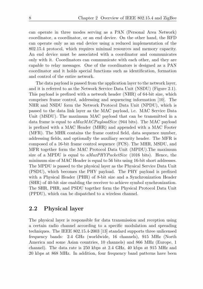
The data payload is passed from the application layer to the network layer,and it is referred to as the Network Service Data Unit (NSDU) (Figure 2.1).This payload is prefixed with a network header (NHR) of 64-bit size, whichcomprises frame control, addressing and sequencing information [10]. TheNHR and NSDU form the Network Protocol Data Unit (NPDU), which ispassed to the data link layer as the MAC payload, i.e. MAC Service DataUnit (MSDU). The maximum MAC payload that can be transmitted in adata frame is equal to aMaxMACPayloadSize (944 bits). The MAC payloadis prefixed with a MAC Header (MHR) and appended with a MAC Footer(MFR). The MHR contains the frame control field, data sequence number,addressing fields, and optionally the auxiliary security header. The MFR iscomposed of a 16-bit frame control sequence (FCS). The MHR, MSDU, andMFR together form the MAC Protocol Data Unit (MPDU).The maximumsize of a MPDU is equal to aMaxPHYPacketSize (1016 bits). Hence, theminimum size of MAC Header is equal to 56 bits using 16-bit short addresses.The MPDU is passed to the physical layer as the Physical Service Data Unit(PSDU), which becomes the PHY payload. The PHY payload is prefixedwith a Physical Header (PHR) of 8-bit size and a Synchronization Header(SHR) of 40-bit size enabling the receiver to achieve symbol synchronization.The SHR, PHR, and PSDU together form the Physical Protocol Data Unit(PPDU), which can be dispatched to a wireless channel.
2.2 Physical layer
The physical layer is responsible for data transmission and reception usinga certain radio channel according to a specific modulation and spreadingtechniques. The IEEE 802.15.4-2003 [13] standard supports three unlicensedfrequency bands: 2.4 GHz (worldwide, 16 channels), 915 MHz (NorthAmerica and some Asian countries, 10 channels) and 866 MHz (Europe, 1channel). The data rate is 250 kbps at 2.4 GHz, 40 kbps at 915 MHz and20 kbps at 868 MHz. In addition, four frequency band patterns have been
2.3 Data link layer 9
Figure 2.1: Structure of the IEEE 802.15.4/ZigBee frames.
added to the 868/915 MHz bands in the last revision of the standard (IEEE802.15.4-2006 [9]). All of these frequency bands are based on the DirectSequence Spread Spectrum (DSSS) or Parallel Sequence Spread Spectrum(PSSS) spreading techniques that have inherently good noise immunity. Thestandard also allows energy detection, link quality indication, clear channelassessment and radio channel switching.
This thesis only considers the 2.4 GHz band with 250 kbps data rate,which is also supported by the TelosB motes [14] used in the experimentaltest-beds. In addition, the Zigbee specification is only defined for thisfrequency band.
2.3 Data link layer
The MAC sub-layer supports the beacon-enabled or non beacon-enabledmodes that may be selected by a central controller of the WSN, i.e. PANcoordinator. In non beacon-enabled mode, the nodes can simply transmitmessages using unslotted Carrier Sense Multiple Access with CollisionAvoidance (CSMA/CA) channel access protocol. In fact, the ”collisionavoidance” mechanism is based on a random delay prior to transmission,which only reduces the probability of collisions. Thus, this mode cannotensure collision-free and predictable access to the shared wireless mediumand, consequently, it cannot provide any time and resource guarantees. Onthe other side, the beacon-enabled mode enables the synchronization of aWSN using periodic beacon frames, the energy conservation using low duty-cycles, and the provision of collision-free and predictable access to the wirelessmedium through the Guaranteed Time Slot (GTS) mechanism. Thus, whenthe timeliness and energy efficiency are the main concerns, the beacon-enabled mode should be employed.
10 Chapter 2 Overview of IEEE 802.15.4 and ZigBee
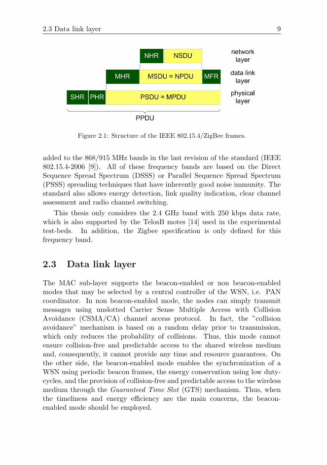
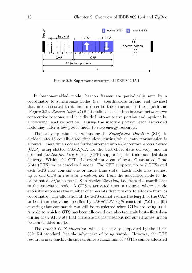
Figure 2.2: Superframe structure of IEEE 802.15.4.
In beacon-enabled mode, beacon frames are periodically sent by acoordinator to synchronize nodes (i.e. coordinators or/and end devices)that are associated to it and to describe the structure of the superframe(Figure 2.2). Beacon Interval (BI) is defined as the time interval between twoconsecutive beacons, and it is divided into an active portion and, optionally,a following inactive portion. During the inactive portion, each associatednode may enter a low power mode to save energy resources.
The active portion, corresponding to Superframe Duration (SD), isdivided into 16 equally-sized time slots, during which data transmission isallowed. These time slots are further grouped into a Contention Access Period(CAP) using slotted CSMA/CA for the best-effort data delivery, and anoptional Contention Free Period (CFP) supporting the time-bounded datadelivery. Within the CFP, the coordinator can allocate Guaranteed TimeSlots (GTS) to its associated nodes. The CFP supports up to 7 GTSs andeach GTS may contain one or more time slots. Each node may requestup to one GTS in transmit direction, i.e. from the associated node to thecoordinator, or/and one GTS in receive direction, i.e. from the coordinatorto the associated node. A GTS is activated upon a request, where a nodeexplicitly expresses the number of time slots that it wants to allocate from itscoordinator. The allocation of the GTS cannot reduce the length of the CAPto less than the value specified by aMinCAPLength constant (7.04 ms [9])ensuring that commands can still be transferred when GTSs are being used.A node to which a GTS has been allocated can also transmit best-effort dataduring the CAP. Note that there are neither beacons nor superframes in nonbeacon-enabled mode.
The explicit GTS allocation, which is natively supported by the IEEE802.15.4 standard, has the advantage of being simple. However, the GTSresources may quickly disappear, since a maximum of 7 GTSs can be allocated
2.3 Data link layer 11
in each superframe. Moreover, the explicit GTS allocation may be notefficient enough in terms of bandwidth utilization, since the bandwidth ofa GTS is given by an integer multiple of the time slot. To overcome theselimitations, the implicit GTS Allocation MEchanism (i-GAME) was proposedby Koubaa et al. [15]. The i-GAME approach enables the use of a GTS byseveral nodes while all their requirements (e.g. bandwidth, delay) are stillsatisfied. For that purpose, the authors have proposed an admission controlalgorithm that enables to decide whether to accept a new GTS allocationrequest or not, based not only on the remaining time slots, but also on thetraffic specifications of the flows, their delay requirements and the availablebandwidth resources. Hence, more than 7 nodes may be associated to acoordinator. On the other hand, the implicit GTS allocation may enlargethe end-to-end delay.
Beacon Interval (BI) and duration of active portion (SD) are defined bytwo parameters, the Beacon Order (BO) and the Superframe Order (SO) asfollows:
BI = aBaseSuperframeDuration · 2BO
SD = aBaseSuperframeDuration · 2SO
for 0 ≤ SO ≤ BO ≤ 14 (2.1)
where aBaseSuperframeDuration = 15.36 ms (assuming the 2.4 GHz fre-quency band with 250 kbps data rate) and denotes the minimum durationof the active portion when SO = 0. The ratio of the active portion (SD) tothe BI is called the duty-cycle. IEEE 802.15.4 standard is optimized for lowduty-cycles (under 1%), which is interesting for the battery-powered nodesto significantly reduce their power consumption. On the other side, low duty-cycle enlarges the end-to-end delays in multi-hop networks such that a fairtrade-off between timeliness and energy efficiency must be found.
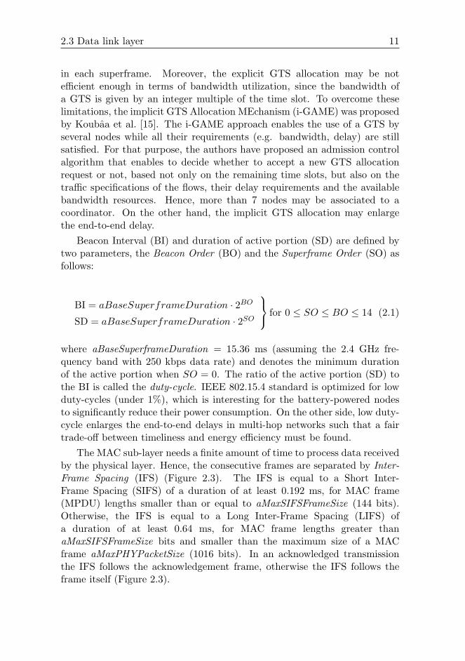
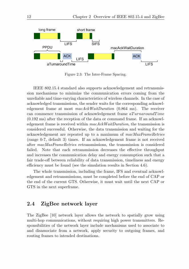
The MAC sub-layer needs a finite amount of time to process data receivedby the physical layer. Hence, the consecutive frames are separated by Inter-Frame Spacing (IFS) (Figure 2.3). The IFS is equal to a Short Inter-Frame Spacing (SIFS) of a duration of at least 0.192 ms, for MAC frame(MPDU) lengths smaller than or equal to aMaxSIFSFrameSize (144 bits).Otherwise, the IFS is equal to a Long Inter-Frame Spacing (LIFS) ofa duration of at least 0.64 ms, for MAC frame lengths greater thanaMaxSIFSFrameSize bits and smaller than the maximum size of a MACframe aMaxPHYPacketSize (1016 bits). In an acknowledged transmissionthe IFS follows the acknowledgement frame, otherwise the IFS follows theframe itself (Figure 2.3).
12 Chapter 2 Overview of IEEE 802.15.4 and ZigBee
Figure 2.3: The Inter-Frame Spacing.
IEEE 802.15.4 standard also supports acknowledgement and retransmis-sion mechanisms to minimize the communication errors coming from theunreliable and time-varying characteristics of wireless channels. In the case ofacknowledged transmissions, the sender waits for the corresponding acknowl-edgement frame at most macAckWaitDuration (0.864 ms). The receivercan commence transmission of acknowledgement frame aTurnaroundT ime(0.192 ms) after the reception of the data or command frame. If an acknowl-edgement frame is received within macAckWaitDuration, the transmission isconsidered successful. Otherwise, the data transmission and waiting for theacknowledgement are repeated up to a maximum of macMaxFrameRetries(range 0-7, default 3) times. If an acknowledgement frame is not receivedafter macMaxFrameRetries retransmissions, the transmission is consideredfailed. Note that each retransmission decreases the effective throughputand increases the communication delay and energy consumption such that afair trade-off between reliability of data transmission, timeliness and energyefficiency must be found (see the simulation results in Section 4.6).
The whole transmission, including the frame, IFS and eventual acknowl-edgement and retransmissions, must be completed before the end of CAP orthe end of the current GTS. Otherwise, it must wait until the next CAP orGTS in the next superframe.
2.4 ZigBee network layer
The ZigBee [10] network layer allows the network to spatially grow usingmulti-hop communications, without requiring high power transmitters. Re-sponsibilities of the network layer include mechanisms used to associate toand disassociate from a network, apply security to outgoing frames, androuting frames to intended destinations.
2.4 ZigBee network layer 13
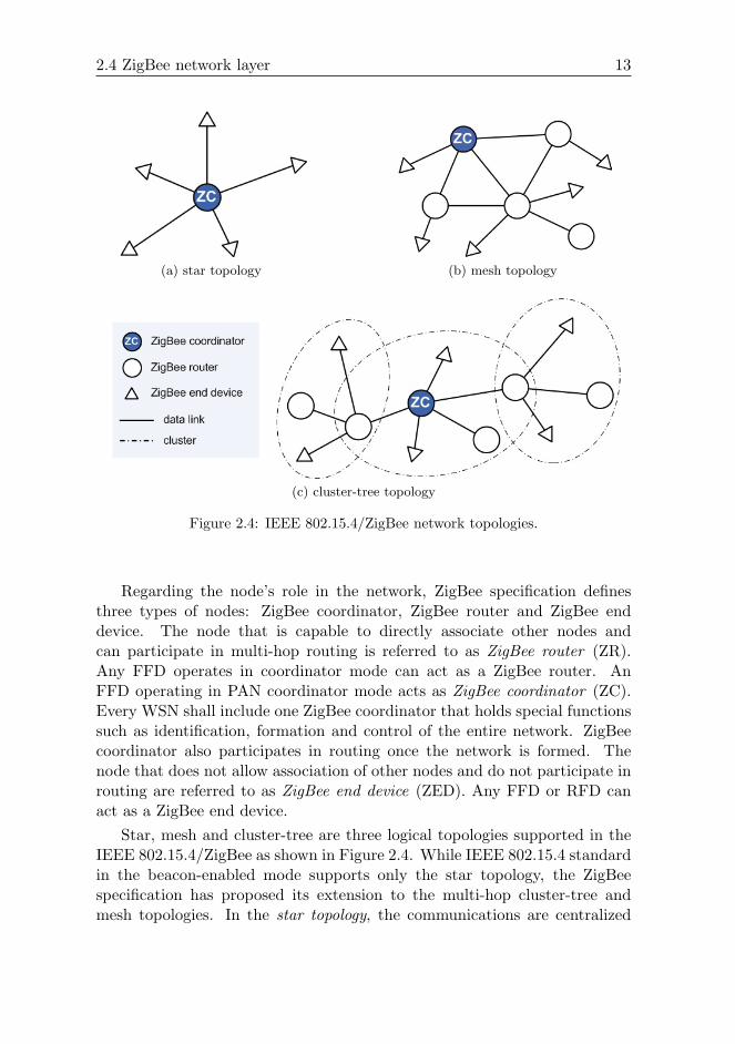
(a) star topology (b) mesh topology
(c) cluster-tree topology
Figure 2.4: IEEE 802.15.4/ZigBee network topologies.
Regarding the node’s role in the network, ZigBee specification definesthree types of nodes: ZigBee coordinator, ZigBee router and ZigBee enddevice. The node that is capable to directly associate other nodes andcan participate in multi-hop routing is referred to as ZigBee router (ZR).Any FFD operates in coordinator mode can act as a ZigBee router. AnFFD operating in PAN coordinator mode acts as ZigBee coordinator (ZC).Every WSN shall include one ZigBee coordinator that holds special functionssuch as identification, formation and control of the entire network. ZigBeecoordinator also participates in routing once the network is formed. Thenode that does not allow association of other nodes and do not participate inrouting are referred to as ZigBee end device (ZED). Any FFD or RFD canact as a ZigBee end device.
Star, mesh and cluster-tree are three logical topologies supported in theIEEE 802.15.4/ZigBee as shown in Figure 2.4. While IEEE 802.15.4 standardin the beacon-enabled mode supports only the star topology, the ZigBeespecification has proposed its extension to the multi-hop cluster-tree andmesh topologies. In the star topology, the communications are centralized
14 Chapter 2 Overview of IEEE 802.15.4 and ZigBee
and established exclusively between a ZigBee coordinator and its associatedZigBee end devices. If a ZED needs to transfer data to another ZED,it sends its data to the ZC, which subsequently forwards the data to theintended recipient. To synchronize the associated ZEDs, the ZC emits regularbeacon frames. Consequently, each ZED can enter a low power mode to savetheir energy whenever it is not active. The ZED can also request for theGTS ensuring predictable and contention-free medium access. The mainadvantages of star topology are its simplicity and predictable and energyefficient behaviour. The drawbacks are limited scalability and ZC as a singlepoint of failure. The ZC’s battery resource can be also rapidly ruined sinceall traffic is routed through ZC. Hence, the star networks are suitable forsimple and small scale applications.
Infrastructure-less mesh topology and infrastructure-based cluster-treetopology allow more complex network formations to be implemented. Themesh topology differs from the star topology in that the communicationsare decentralized and any node can directly communicate with any othernode within its radio range. The mesh network usually operates in ad hocfashion that induces unpredictable end-to-end connectivity between nodes. Incontrast with the star topology, the mesh topology provides good scalabilityand enhanced network flexibility such as redundant routing paths thatincreases end-to-end reliability of data transmission and ensures fair resourceusage. In addition, this communication redundancy can eliminate single pointof failure. On the other hand, the probabilistic routing protocol (e.g. Ad hocOn Demand Distance Vector (AODV) routing protocol defined in ZigBee)and contention-based MAC protocol cause unpredictable performance andresource bounds. Moreover, since the routing paths cannot be predicted inadvance, the nodes cannot enter low power mode which leads to a uselesswaste of energy.
The cluster-tree topology combines the benefits of both above mentionedtopologies such as good scalability, network synchronization and predictableand energy efficient behaviour, which is suited for medium-scale time-sensitive applications using battery-powered nodes. Cluster-tree is tree-basedtopology, where the nodes are organized in logical groups, called clusters.Each router (including ZigBee coordinator) forms a cluster and is referred toas its cluster-head. All nodes associated with a given cluster-head belong toits cluster, and the cluster-head handles all their transmissions. Note thateach cluster can be seen as a star subnetwork. ZigBee coordinator is identifiedas the root of the tree and forms the initial cluster. The other ZigBeerouters join the cluster-tree in turn by establishing themselves as cluster-heads, starting to generate the beacon frames for their own clusters. Contrary
2.4 ZigBee network layer 15
to the mesh topology, there is a single routing path between any pair of nodesin a cluster-tree topology. Hence, multi-hop communication is deterministicand time efficient because each node only interacts with its predefinedset of nearby nodes. The deterministic routing protocol and contention-free medium access (GTS) ensure predictable network performance andresource bounds. In addition, thanks to the deterministic routing andsynchronous behaviour in cluster-tree topology, the nodes know their activetime in advance. Hence, each node can save its energy by entering thelow power mode when it does not participate in the routing. Contrary tothe mesh network, the cluster-tree network is less flexible since it relies onthe pre-deployed infrastructure. The cluster-tree network also needs specificalgorithms to correctly design the parameters that regulate beacon and datatransmission in order to achieve a good network capacity. Clearly, thebehaviour of the whole cluster-tree network strongly depends on the settingof the parameters. For example, if SO = BO there will be no inactive portionmeaning that the nodes cannot enter into the low power mode and, on theother hand, if SO is set too low (and so does the duty-cycle), the data ratehas to be decreased.
star mesh cluster-tree
scalability no yes yes
energy efficiency yes no yes
network synchronization yes no yes
redundant paths no yes no
node mobility partial yes partial
deterministic routing yes no yes
contention-free medium access yes no yes
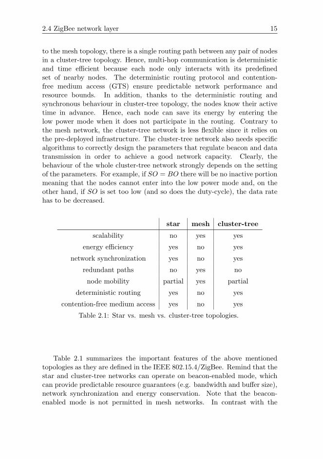
Table 2.1: Star vs. mesh vs. cluster-tree topologies.
Table 2.1 summarizes the important features of the above mentionedtopologies as they are defined in the IEEE 802.15.4/ZigBee. Remind that thestar and cluster-tree networks can operate on beacon-enabled mode, whichcan provide predictable resource guarantees (e.g. bandwidth and buffer size),network synchronization and energy conservation. Note that the beacon-enabled mode is not permitted in mesh networks. In contrast with the

16 Chapter 2 Overview of IEEE 802.15.4 and ZigBee
star and mesh networks, the cluster-tree network requires precise clusterscheduling (Chapter 4) to avoid inter-cluster collisions (messages/beaconstransmitted from nodes in different overlapping clusters). IEEE 802.15.4standard and Zigbee specification admit the formation of the cluster-treenetwork but none of them imposes any algorithm or methodology to createor organize it. Thus, the cluster-tree topology expresses several challengingand open research issues in this area, which have been addresses in this thesis.
Chapter 3
IEEE 802.15.4/ZigBeesimulation model:delay/throughput evaluationof the GTS mechanism
3.1 Introduction
Simulation and modelling are important approaches to developing andevaluating the systems in terms of time and cost. A simulation showsthe expected behaviour of a system based on its simulation model underdifferent conditions. To study system behaviour and performance by meansof real deployment or setting up a test-bed may require much effort, time andfinancial costs. However, the simulation results are not necessarily accurateor representative. Hence, the goal for any simulation model is to accuratelymodel and predict the behaviour of a real system.
Recently, several analytical and simulation models of the IEEE 802.15.4 [9]protocol have been proposed. Nevertheless, currently available simulationmodels [16] for this protocol are both inaccurate and incomplete, and inparticular they do not support the Guaranteed Time Slot (GTS) mechanism,which is required for time-sensitive wireless sensor applications.
This chapter presents an accurate IEEE 802.15.4/ZigBee simulationmodel developed in the Opnet Modeler simulator [17]. Opnet Modeler waschosen due to its accuracy and to its sophisticated graphical user interface.The idea behind this simulation model was triggered by the need to build a
17
18 Chapter 3 IEEE 802.15.4/ZigBee simulation model
very reliable model of the IEEE 802.15.4 and ZigBee protocols for WirelessSensor Networks (WSNs). The simulation model is validated with focuson the GTS mechanism using the the Network Calculus based analyticalmodel [11]. The results previously obtained through Network Calculus upperbound or overpass the results obtained through simulation. The tightersimulation results allow to propose a novel methodology to tune the protocolparameters such that a better performance of the protocol can be guaranteed.
Contribution
The motivation that has driven this work was the performance evaluationof the real-time behaviour of the IEEE 802.15.4/ZigBee beacon-enabledcluster-tree WSNs. Thus, this chapter contributes an accurate Opnetsimulation model for the IEEE 802.15.4 and ZigBee protocols focusing onthe implementation of the GTS mechanism and ZigBee hierarchical routingstrategy. The simulation model is used to carry out a set of experiments andto compare the performance evaluation of the GTS mechanism as given bythe two alternative approaches, namely simulation and analytical.
Additionally, and probably more importantly, based on the simulationmodel a novel methodology is proposed to tune the IEEE 802.15.4 parameters(e.g. SO, BO) such that a better performance of the IEEE 802.15.4 protocolcan be guaranteed, both concerning maximizing the throughput of theallocated GTS as well as concerning minimizing media access delay.
In particular, the Chapter 3 presents the following contributions:
1. An accurate simulation model of IEEE 802.15.4/ZigBee protocols thathas been implemented in the Opnet network simulator.
2. A demonstration of the validity of proposed simulation model throughan analytical model based on Network Calculus.
3. A novel methodology to tune the IEEE 802.15.4 parameters such thata better performance can be guaranteed.
3.2 Related work
Opnet Modeler, ns-2 and OMNeT++ are widely used and popular networksimulators which, among others, include a simulation model of the IEEE802.15.4 protocol. Of course, each simulator has its own disadvantagesand advantages. The 802.15.4/ZigBee simulation model in Opnet model
3.2 Related work 19
library [17] supports only non beacon-enabled mode, therefore, the cluster-tree topology and GTS mechanism cannot be simulated. In addition, thesource codes of the network and application layers are not available. TheNational Institute of Standards and Technology (NIST) has developed ownOpnet simulation model for the IEEE 802.15.4 protocol [18]. However,while that model implements the slotted and the unslotted CSMA/CA MACprotocols it does not support the GTS mechanism as well. It also uses itsown radio channel model rather than the accurate Opnet wireless library.The Network Simulator 2 (ns-2) [19] is an object-oriented discrete eventsimulator including a simulation model of the IEEE 802.15.4 protocol. Theaccuracy of its simulation results is questionable since the MAC protocols,packet formats, and energy models are very different from those usedin real WSNs [20]. This basically results from the facts that ns-2 wasoriginally developed for IP-based networks and further extended for wirelessnetworks. Moreover, the GTS mechanism was not implemented in the ns-2model. OMNeT++ (Objective Modular Network Test-bed in C++) [21] isanother discrete event network simulator supporting unslotted IEEE 802.15.4CSMA/CA MAC protocol only. Finally, note that while ns-2 and OMNeT++are open source projects, the Opnet Modeler is commercial project providinga free of charge university program for academic research projects.
There have also been several research works on the performance evalua-tion of the IEEE 802.15.4 protocol using simulation model. Zheng et al. [22]have evaluated various features of the 802.15.4 protocol (e.g. direct, indirectand GTS data transmissions), and investigated the collision behaviourof IEEE 802.15.4. In addition, the simulation experiments compare theperformance of 802.15.4 and 802.11 (WiFi) protocols. The authors havedeveloped own ns-2 simulation model of 802.15.4 protocol, which additionallyimplements beacon-enabled mode and GTS mechanism. Since the networklayer has not been implemented, a star topology is only supported. Based onthis implementation, Chen et al. [23] have developed own simulation model ofIEEE 802.15.4 protocol in OMNeT++. Contrary to the standard OMNeT++model, their simulation model implements a battery module, beacon-enabledmode and GTS mechanism, and supports only star topology. Using thissimulation model, the IEEE 802.15.4 star network has been evaluated interms of energy consumption and end-to-end communication performancein [24]. Hurtado-Lopez et al. [25] have extended the above mentioned IEEE802.15.4 model in OMNeT++ to support cluster-tree topology.
In [26], the authors have presented a simulation study of the slottedCSMA/CA MAC protocol deployed by the IEEE 802.15.4 protocol in beacon-enabled mode, using the previous version of the Opnet simulation model. In

20 Chapter 3 IEEE 802.15.4/ZigBee simulation model
this chapter, this version has been extend to include the GTS mechanismand ZigBee network layer, which allows a simulation study of the real-timebehaviour of cluster-tree WSNs.
3.3 Simulation model
This section presents the structure of the IEEE 802.15.4/ZigBee simulationmodel [27] that was implemented in the Opnet Modeler simulator.
3.3.1 Simulation model structure
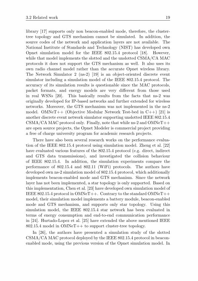
The Opnet Modeler [17] is a commercial discrete-event network modellingand simulation environment, which provides tools for all phases of a systemanalysis and testing cycle including model design, simulation, data collectionand data analysis. Both behaviour and performance of modelled systemscan be analysed and visualized in a rich integrated graphical environment.Opnet’s Standard Model Library supports hundreds of generic or vendor-specific protocols and technologies that can be use to build the networks.In addition, Opnet Modeler simulator includes a hierarchical developmentenvironment to enable modelling of any type of custom protocol anddevice. The development environment consists of three hierarchical modellingdomains (Figure 3.1). Network domain describes network topology in termsof nodes and links. Internal architecture of a node is described in the nodedomain. Within the process domain, the behaviour of a node is defined usingstate transition diagrams. Operations performed in each state or transitionare described in embedded C/C++ code blocks. The IEEE 802.15.4/ZigBeesimulation model builds on the wireless module, an add-on that extends thefunctionality of the Opnet Modeler with accurate modelling, simulation andanalysis of wireless networks.
The IEEE 802.15.4/ZigBee Opnet simulation model implements physicallayer and medium access control sub-layer defined in IEEE 802.15.4 [9]standard, and network layer defined in ZigBee [10] specification. The latestversion of simulation model [27] supports the following features:
– beacon-enabled mode (beacon frame generation)– star and cluster-tree topologies– computation of the power consumption (MICAz and TelosB motes are
supported)– physical layer characteristics– slotted CSMA/CA MAC protocol
3.3 Simulation model 21
Figure 3.1: The structure of the IEEE 802.15.4/ZigBee Opnet simulation model.
– Guaranteed Time Slot (GTS) mechanism (GTS allocation, deallocationand reallocation functions)
– generation of the acknowledged or unacknowledged best-effort applica-tion data (MSDU) transmitted during the CAP
– generation of the acknowledged or unacknowledged real-time applica-tion data transmitted during the CFP
– ZigBee hierarchical tree routing– verification of node’s address that must correspond to the ZigBee
hierarchical addressing scheme
In accordance to the ZigBee [10] specification, there are implementedthree types of nodes in the simulation model, namely a ZigBee coordinator,a ZigBee router and a ZigBee end device. All types of nodes have the sameinternal architecture (node domain) but they differ in the available user-defined attributes (Section 3.3.2).
The structure of the IEEE 802.15.4/ZigBee simulation model is presentedin Figure 3.1. The the physical layer consists of a wireless radio transmitterand receiver compliant to the IEEE 802.15.4 [9] standard running at 2.4 GHz

22 Chapter 3 IEEE 802.15.4/ZigBee simulation model
frequency band with 250 kbps data rate. Default settings are used for thephysical characteristics of the radio channel such as background noise andinterference, propagation delay, antenna gain, and bit error rate.
The data link layer supports the beacon-enabled mode (non beacon-enabled mode is not supported yet) and implements two medium accesscontrol protocols according to the IEEE 802.15.4 standard, namely thecontention-based slotted CSMA/CA and contention-free GTS. MAC payload(MSDU) incoming from the network layer is wrapped in MAC header andMAC footer and stored into two separate FIFO buffers, namely a buffer forbest-effort data frames and another buffer for real-time data frames. Theframes are dispatched to the network when the corresponding CAP or CFPis active. On the other hand, the frame (MPDU) incoming from the physicallayer is unwrapped and passed to the network layer for further processing.The data link layer also generates required commands (e.g. GTS allocation,deallocation and reallocation commands) and beacon frames when a nodeacts as PAN coordinator or router.
The network layer implements address-based tree routing (a mesh routingis not supported yet) according to the ZigBee [10] specification. The framesare routed upward or downward along the cluster-tree topology accordingto the destination address by exploiting the hierarchical addressing schemeprovided by ZigBee [10]. This addressing scheme assigns an unique addressto each node using the symmetric hierarchical addressing tree given by threeparameters, namely the maximum number of children (i.e. routers and enddevices) that a router or a coordinator may have (Cm), the maximum depthin the topology (Lm), and the maximum number of routers that a router ora coordinator may have as children (Rm).
The application layer can generate unacknowledged and/or acknowledgedbest-effort and/or real-time data frames transmitted during CAP or CFP,respectively. There is also a battery module that computes the consumed andremaining energy levels. The default values of current draws are set to thoseof the widely-used MICAz [28] or TelosB [14] motes.
3.3.2 User-defined attributes
This section depicts some important user-defined attributes relating to theGTS mechanism and the real-time data traffic. All attributes are describedin the reference guide [29] in details.
A coordinator and each router may accept or reject the GTS allocationrequest from its children according to the value of the attribute GTS Permit.Each node (except the coordinator) can specify the time when the GTS
3.3 Simulation model 23
Figure 3.2: The user-defined attributes of the GTS mechanism.
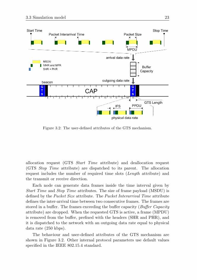
allocation request (GTS Start Time attribute) and deallocation request(GTS Stop Time attribute) are dispatched to its parent. The allocationrequest includes the number of required time slots (Length attribute) andthe transmit or receive direction.
Each node can generate data frames inside the time interval given byStart Time and Stop Time attributes. The size of frame payload (MSDU) isdefined by the Packet Size attribute. The Packet Interarrival Time attributedefines the inter-arrival time between two consecutive frames. The frames arestored in a buffer. The frames exceeding the buffer capacity (Buffer Capacityattribute) are dropped. When the requested GTS is active, a frame (MPDU)is removed from the buffer, prefixed with the headers (SHR and PHR), andit is dispatched to the network with an outgoing data rate equal to physicaldata rate (250 kbps).
The behaviour and user-defined attributes of the GTS mechanism areshown in Figure 3.2. Other internal protocol parameters use default valuesspecified in the IEEE 802.15.4 standard.
24 Chapter 3 IEEE 802.15.4/ZigBee simulation model
3.4 Simulation setup
In this chapter, a simple star network containing a coordinator and oneassociated end device is considered. This configuration is sufficient for theperformance evaluation of the GTS mechanism, since there is no medium ac-cess contention inside the GTS. Thus, having additional nodes would have noinfluence on the simulation results. Next, the unacknowledged transmission(macMaxFrameRetries = 0) is only considered for comparative purposeswith the analytical results obtained in [11].
For the sake of simplicity, and without loss of generality, we assume theallocation of only one time slot GTS in transmit direction and a 100% duty-cycle (i.e. SO = BO). In what follows, the change of the SO means that theBO also changes while satisfying SO = BO. This means that the optionalinactive portion is not included in the superframe.
Reliability of data transmission may be enhanced by keeping the framesize as small as practical, as this gives the highest probability of a frame beingdelivered in the presence of interference. Prolonged battery life is achievedby minimizing the on duration of the radio (receive and transmit modes),where most power is consumed [30]. A small frame size and infrequenttransmission both help to achieve this. Hence, small frame sizes are usedduring the simulation (i.e. Packet Size = 40 or 41 bits).
The statistical data (e.g. average, maximum, minimum delays) arecomputed from a set of 1000 samples. Hence, the simulation time of onerun is equal to the duration of 1000 superframe periods and, consequently,the simulation time depends on the Superframe Order (SO).
3.4.1 Simulation vs. analytical models
In Section 3.5, the performance of the GTS mechanism from the Opnetsimulation model is evaluated against the analytical model of the GTSmechanism proposed in [11], which is based on the Network Calculusformalism. Network Calculus (Section 5.3) is a mathematical methodologybased on min-plus algebra that applies to the deterministic analysis ofqueuing/flows in communication networks.
The Network Calculus based analytical model relies on the affine arrivalcurve and rate-latency service curve [31]. This means that each generatedapplication data flow has a cumulative arrival function R(t) upper boundedby the affine arrival curve αb,r(t) = b+r·t, where b denotes the burst toleranceand r denotes the average arrival rate. The analytical model is bit-oriented,which means that the application data are generated as a continuous bit
3.5 Performance evaluation 25
stream with data rate r. On the other side, the simulation model has amore realistic frame-oriented basis, where the frames with a specified size aregenerated with a given period (refer to Figure 3.2). Consequently, the bursttolerance b and arrival rate r, as defined in the analytical model, should beimplemented in the simulation model in the following way. A FIFO bufferwith a specified capacity substitutes a data burst with a given size, and thearrival data rate is defined as follows:
r =Packet size
Packet Interarrival T ime[bps] (3.1)
The smallest data unit in the analytical model is a bit, while in thesimulation model it is a frame with a bounded size.
3.5 Performance evaluation
This section shows how the Superframe Order, the arrival data rate, thebuffer capacity and the size of the frame payload impact the throughput ofthe allocated GTS and the media access delay of the transmitted frames.
3.5.1 Impact of the Superframe Order on the GTSthroughput
Throughput as a function of the arrival data rate
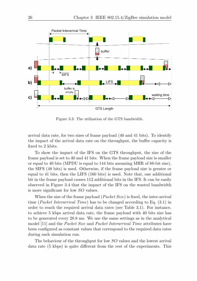
The purpose of this section is to evaluate and compare the data throughputduring one time slot GTS, for different values of the Superframe Order and fordifferent arrival rates. For a given SO, the data throughput is related to thetime effectively used for data transmission inside the GTS. Since the framesare transmitted without acknowledgement, the wasted bandwidth can onlyresult from IFS or waiting for a new frame if the buffer is empty, as depictedin Figure 3.3.
The frames can be dispatched at the physical data rate (250 kbps) ifthe buffer does not become empty before the end of GTS (Figure 3.3a, b).Otherwise, if the buffer becomes empty, the frames are not stored in thebuffer but they are directly dispatched to the network according to theirarrival data rate Eq. (3.1), which is often lower than the physical data rate(Figure 3.3c).
Figure 3.4 plots the average data throughput of allocated one time slotGTS for different SOs (with a duty-cycle equal to 1) as a function of the
26 Chapter 3 IEEE 802.15.4/ZigBee simulation model
Figure 3.3: The utilization of the GTS bandwidth.
arrival data rate, for two sizes of frame payload (40 and 41 bits). To identifythe impact of the arrival data rate on the throughput, the buffer capacity isfixed to 2 kbits.
To show the impact of the IFS on the GTS throughput, the size of theframe payload is set to 40 and 41 bits. When the frame payload size is smalleror equal to 40 bits (MPDU is equal to 144 bits assuming MHR of 88-bit size),the SIFS (48 bits) is used. Otherwise, if the frame payload size is greater orequal to 41 bits, then the LIFS (160 bits) is used. Note that, one additionalbit in the frame payload causes 112 additional bits in the IFS. It can be easilyobserved in Figure 3.4 that the impact of the IFS on the wasted bandwidthis more significant for low SO values.
When the size of the frame payload (Packet Size) is fixed, the inter-arrivaltime (Packet Interarrival Time) has to be changed according to Eq. (3.1) inorder to reach the required arrival data rates (see Table 3.1). For instance,to achieve 5 kbps arrival data rate, the frame payload with 40 bits size hasto be generated every 28.8 ms. We use the same settings as in the analyticalmodel [11] and the Packet Size and Packet Interarrival Time attributes havebeen configured as constant values that correspond to the required data ratesduring each simulation run.
The behaviour of the throughput for low SO values and the lowest arrivaldata rate (5 kbps) is quite different from the rest of the experiments. This
3.5 Performance evaluation 27
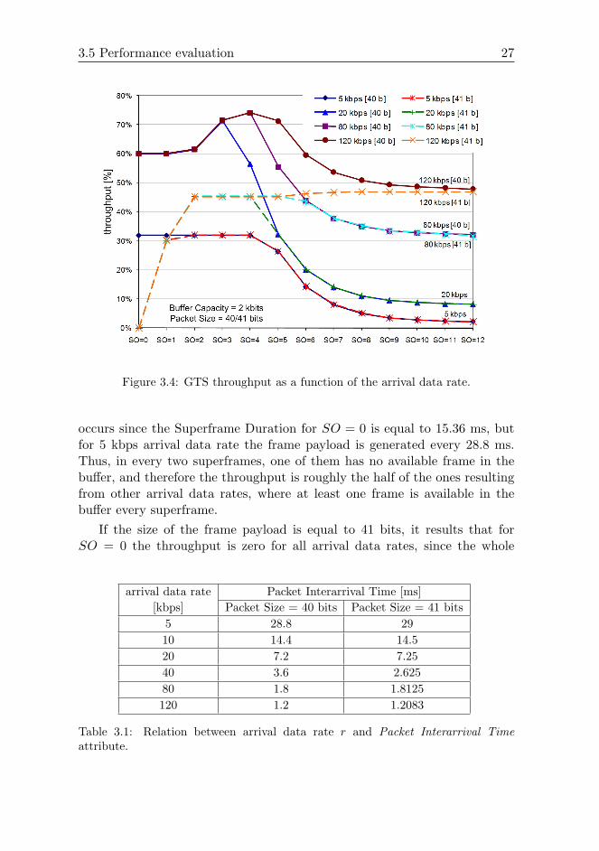
Figure 3.4: GTS throughput as a function of the arrival data rate.
occurs since the Superframe Duration for SO = 0 is equal to 15.36 ms, butfor 5 kbps arrival data rate the frame payload is generated every 28.8 ms.Thus, in every two superframes, one of them has no available frame in thebuffer, and therefore the throughput is roughly the half of the ones resultingfrom other arrival data rates, where at least one frame is available in thebuffer every superframe.
If the size of the frame payload is equal to 41 bits, it results that forSO = 0 the throughput is zero for all arrival data rates, since the whole
arrival data rate Packet Interarrival Time [ms][kbps] Packet Size = 40 bits Packet Size = 41 bits
5 28.8 2910 14.4 14.520 7.2 7.2540 3.6 2.62580 1.8 1.8125120 1.2 1.2083
Table 3.1: Relation between arrival data rate r and Packet Interarrival Timeattribute.
28 Chapter 3 IEEE 802.15.4/ZigBee simulation model
Figure 3.5: GTS throughput as a function of the arrival data rate: simulation vs.analytical model.
transmission (including the frame and LIFS) cannot be completed before theend of the GTS.
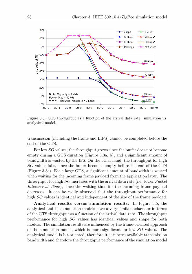
For low SO values, the throughput grows since the buffer does not becomeempty during a GTS duration (Figure 3.3a, b), and a significant amount ofbandwidth is wasted by the IFS. On the other hand, the throughput for highSO values falls, since the buffer becomes empty before the end of the GTS(Figure 3.3c). For a large GTS, a significant amount of bandwidth is wastedwhen waiting for the incoming frame payload from the application layer. Thethroughput for high SO increases with the arrival data rate (i.e. lower PacketInterarrival Time), since the waiting time for the incoming frame payloaddecreases. It can be easily observed that the throughput performance forhigh SO values is identical and independent of the size of the frame payload.
Analytical results versus simulation results. In Figure 3.5, theanalytical and the simulation models have a very similar behaviour in termsof the GTS throughput as a function of the arrival data rate. The throughputperformance for high SO values has identical values and shape for bothmodels. The simulation results are influenced by the frame-oriented approachof the simulation model, which is more significant for low SO values. Theanalytical model is bit-oriented, therefore it saturates available transmissionbandwidth and therefore the throughput performance of the simulation model
3.5 Performance evaluation 29
Figure 3.6: GTS throughput as a function of the buffer capacity.
is upper bounded by the maximum throughput of the analytical model(analytical results are drawn with dashed lines).
Throughput as a function of the buffer capacity
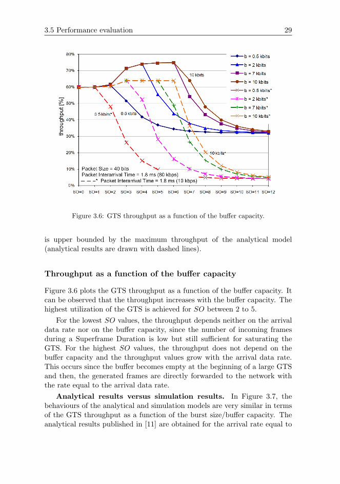
Figure 3.6 plots the GTS throughput as a function of the buffer capacity. Itcan be observed that the throughput increases with the buffer capacity. Thehighest utilization of the GTS is achieved for SO between 2 to 5.
For the lowest SO values, the throughput depends neither on the arrivaldata rate nor on the buffer capacity, since the number of incoming framesduring a Superframe Duration is low but still sufficient for saturating theGTS. For the highest SO values, the throughput does not depend on thebuffer capacity and the throughput values grow with the arrival data rate.This occurs since the buffer becomes empty at the beginning of a large GTSand then, the generated frames are directly forwarded to the network withthe rate equal to the arrival data rate.
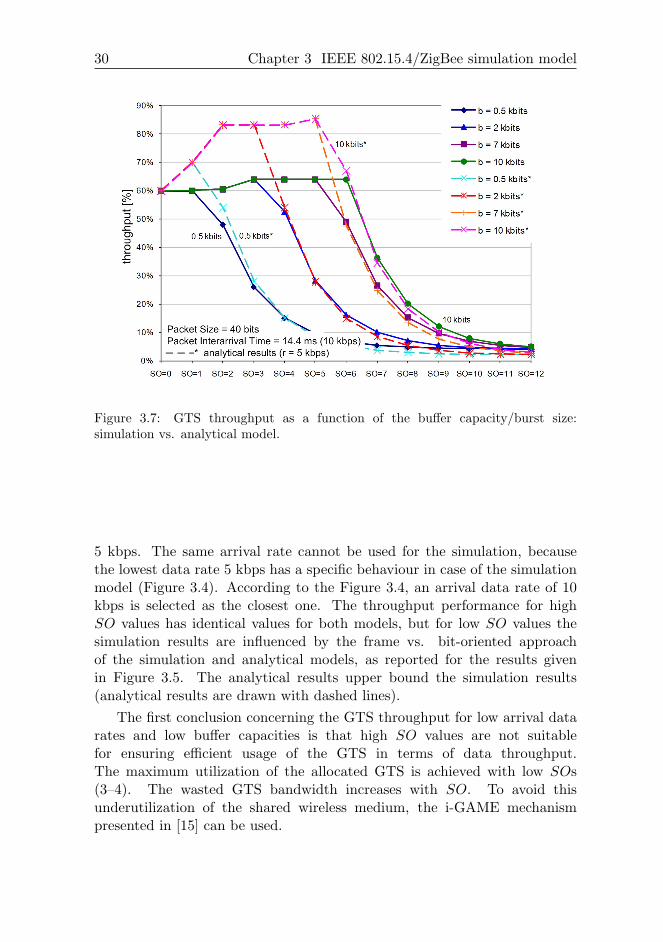
Analytical results versus simulation results. In Figure 3.7, thebehaviours of the analytical and simulation models are very similar in termsof the GTS throughput as a function of the burst size/buffer capacity. Theanalytical results published in [11] are obtained for the arrival rate equal to
30 Chapter 3 IEEE 802.15.4/ZigBee simulation model
Figure 3.7: GTS throughput as a function of the buffer capacity/burst size:simulation vs. analytical model.
5 kbps. The same arrival rate cannot be used for the simulation, becausethe lowest data rate 5 kbps has a specific behaviour in case of the simulationmodel (Figure 3.4). According to the Figure 3.4, an arrival data rate of 10kbps is selected as the closest one. The throughput performance for highSO values has identical values for both models, but for low SO values thesimulation results are influenced by the frame vs. bit-oriented approachof the simulation and analytical models, as reported for the results givenin Figure 3.5. The analytical results upper bound the simulation results(analytical results are drawn with dashed lines).
The first conclusion concerning the GTS throughput for low arrival datarates and low buffer capacities is that high SO values are not suitablefor ensuring efficient usage of the GTS in terms of data throughput.The maximum utilization of the allocated GTS is achieved with low SOs(3–4). The wasted GTS bandwidth increases with SO. To avoid thisunderutilization of the shared wireless medium, the i-GAME mechanismpresented in [15] can be used.
3.5 Performance evaluation 31
3.5.2 Impact of the Superframe Order on the media accessdelay
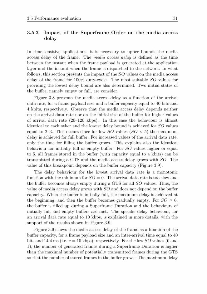
In time-sensitive applications, it is necessary to upper bounds the mediaaccess delay of the frame. The media access delay is defined as the timebetween the instant when the frame payload is generated at the applicationlayer and the instant when the frame is dispatched to the network. In whatfollows, this section presents the impact of the SO values on the media accessdelay of the frame for 100% duty-cycle. The most suitable SO values forproviding the lowest delay bound are also determined. Two initial states ofthe buffer, namely empty or full, are consider.
Figure 3.8 presents the media access delay as a function of the arrivaldata rate, for a frame payload size and a buffer capacity equal to 40 bits and4 kbits, respectively. Observe that the media access delay depends neitheron the arrival data rate nor on the initial size of the buffer for higher valuesof arrival data rate (20–120 kbps). In this case the behaviour is almostidentical to each other and the lowest delay bound is achieved for SO valuesequal to 2–3. This occurs since for low SO values (SO < 5) the maximumdelay is achieved for full buffer. For increased values of the arrival data rate,only the time for filling the buffer grows. This explains also the identicalbehaviour for initially full or empty buffer. For SO values higher or equalto 5, all frames stored in the buffer (with capacity equal to 4 kbits) can betransmitted during a GTS and the media access delay grows with SO. Thevalue of this breakpoint depends on the buffer capacity (Figure 3.9).
The delay behaviour for the lowest arrival data rate is a monotonicfunction with the minimum for SO = 0. The arrival data rate is too slow andthe buffer becomes always empty during a GTS for all SO values. Thus, thevalue of media access delay grows with SO and does not depend on the buffercapacity. When the buffer is initially full, the maximum delay is achieved atthe beginning, and then the buffer becomes gradually empty. For SO ≥ 6,the buffer is filled up during a Superframe Duration and the behaviours ofinitially full and empty buffers are met. The specific delay behaviour, foran arrival data rate equal to 10 kbps, is explained in more details, with thesupport of the results shown in Figure 3.9.
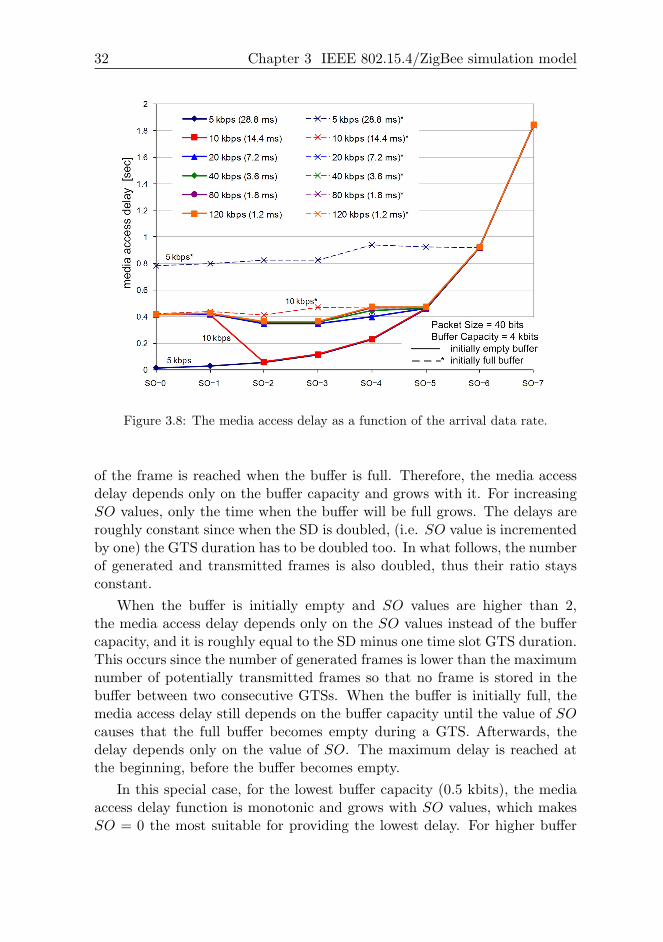
Figure 3.9 shows the media access delay of the frame as a function of thebuffer capacity, for a frame payload size and an inter-arrival time equal to 40bits and 14.4 ms (i.e. r = 10 kbps), respectively. For the low SO values (0 and1), the number of generated frames during a Superframe Duration is higherthan the maximal number of potentially transmitted frames during the GTSso that the number of stored frames in the buffer grows. The maximum delay
32 Chapter 3 IEEE 802.15.4/ZigBee simulation model
Figure 3.8: The media access delay as a function of the arrival data rate.
of the frame is reached when the buffer is full. Therefore, the media accessdelay depends only on the buffer capacity and grows with it. For increasingSO values, only the time when the buffer will be full grows. The delays areroughly constant since when the SD is doubled, (i.e. SO value is incrementedby one) the GTS duration has to be doubled too. In what follows, the numberof generated and transmitted frames is also doubled, thus their ratio staysconstant.
When the buffer is initially empty and SO values are higher than 2,the media access delay depends only on the SO values instead of the buffercapacity, and it is roughly equal to the SD minus one time slot GTS duration.This occurs since the number of generated frames is lower than the maximumnumber of potentially transmitted frames so that no frame is stored in thebuffer between two consecutive GTSs. When the buffer is initially full, themedia access delay still depends on the buffer capacity until the value of SOcauses that the full buffer becomes empty during a GTS. Afterwards, thedelay depends only on the value of SO. The maximum delay is reached atthe beginning, before the buffer becomes empty.
In this special case, for the lowest buffer capacity (0.5 kbits), the mediaaccess delay function is monotonic and grows with SO values, which makesSO = 0 the most suitable for providing the lowest delay. For higher buffer
3.5 Performance evaluation 33
Figure 3.9: The media access delay as a function of the buffer capacity.
capacities, the most suitable value of SO in terms of the lowest delay isdefinitely 2 and does not depend on the buffer capacity, when the buffer isinitially empty.
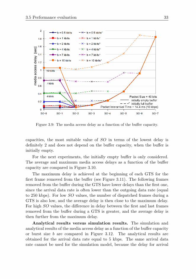
For the next experiments, the initially empty buffer is only considered.The average and maximum media access delays as a function of the buffercapacity are compared in Figure 3.10.
The maximum delay is achieved at the beginning of each GTS for thefirst frame removed from the buffer (see Figure 3.11). The following framesremoved from the buffer during the GTS have lower delays than the first one,since the arrival data rate is often lower than the outgoing data rate (equalto 250 kbps). For low SO values, the number of dispatched frames during aGTS is also low, and the average delay is then close to the maximum delay.For high SO values, the difference in delay between the first and last framesremoved from the buffer during a GTS is greater, and the average delay isthen further from the maximum delay.
Analytical results versus simulation results. The simulation andanalytical results of the media access delay as a function of the buffer capacityor burst size b are compared in Figure 3.12. The analytical results areobtained for the arrival data rate equal to 5 kbps. The same arrival datarate cannot be used for the simulation model, because the delay for arrival
34 Chapter 3 IEEE 802.15.4/ZigBee simulation model
Figure 3.10: Average vs. maximum media access delay as a function of the buffercapacity.
data rate equal to 5 kbps does not depend on the buffer capacity (Figure 3.8).According to the results shown in Figure 3.8, the arrival data rate equal to20 kbps has been selected as the closest one. Hence, we cannot compare thevalues, but only the behaviour of the models in terms of media access delay.This behaviour is roughly similar for both models, and the lowest delay isachieved for SO = 2 for the case of higher buffer capacity (2–10 kbits), orfor SO = 0 in case of lower buffer capacity (0.5 and 1 kbits). The differencebetween frame-oriented and bit-oriented approaches of the simulation andanalytical models, respectively, can be observed for the higher SO values. Incase of the analytical model, the delay curves converge slowly into a singleone (analytical results are drawn with dashed lines).
In summary, WSN applications with low data rates and low buffercapacities achieve the lowest delay bound for SO = 0. However, for higherbuffer capacities (more than 1 kbits) and higher arrival data rates (more than10 kbps) the most suitable value of SO for providing real-time guaranteesis 2. The simulation and analytical results are roughly identical in terms ofthe media access delay, and the simulation results are upper bounded by theanalytical results.
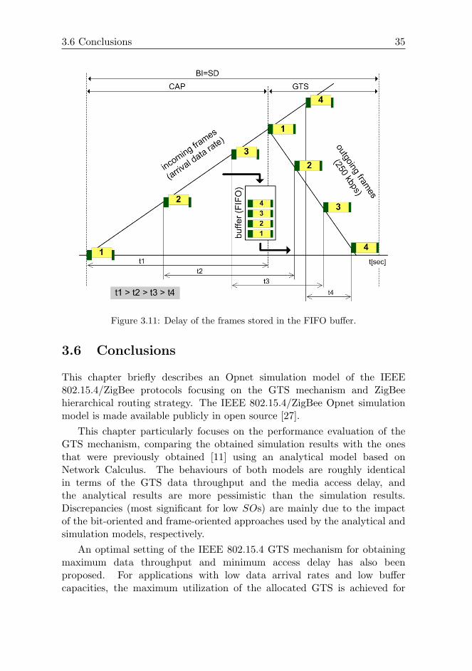
3.6 Conclusions 35
Figure 3.11: Delay of the frames stored in the FIFO buffer.
3.6 Conclusions
This chapter briefly describes an Opnet simulation model of the IEEE802.15.4/ZigBee protocols focusing on the GTS mechanism and ZigBeehierarchical routing strategy. The IEEE 802.15.4/ZigBee Opnet simulationmodel is made available publicly in open source [27].
This chapter particularly focuses on the performance evaluation of theGTS mechanism, comparing the obtained simulation results with the onesthat were previously obtained [11] using an analytical model based onNetwork Calculus. The behaviours of both models are roughly identicalin terms of the GTS data throughput and the media access delay, andthe analytical results are more pessimistic than the simulation results.Discrepancies (most significant for low SOs) are mainly due to the impactof the bit-oriented and frame-oriented approaches used by the analytical andsimulation models, respectively.
An optimal setting of the IEEE 802.15.4 GTS mechanism for obtainingmaximum data throughput and minimum access delay has also beenproposed. For applications with low data arrival rates and low buffercapacities, the maximum utilization of the allocated GTS is achieved for
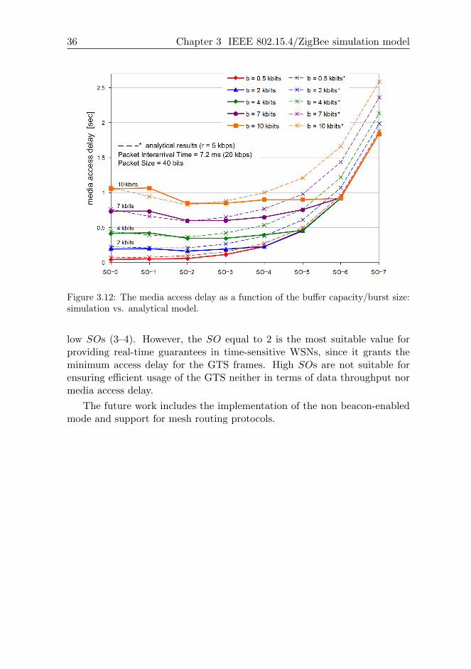
36 Chapter 3 IEEE 802.15.4/ZigBee simulation model
Figure 3.12: The media access delay as a function of the buffer capacity/burst size:simulation vs. analytical model.
low SOs (3–4). However, the SO equal to 2 is the most suitable value forproviding real-time guarantees in time-sensitive WSNs, since it grants theminimum access delay for the GTS frames. High SOs are not suitable forensuring efficient usage of the GTS neither in terms of data throughput normedia access delay.
The future work includes the implementation of the non beacon-enabledmode and support for mesh routing protocols.
Chapter 4
Energy efficient schedulingfor cluster-tree WirelessSensor Networks withtime-bounded data flows
4.1 Introduction
This chapter assumes a static deployment of wireless nodes organized inthe cluster-tree topology along with the set of periodic time-bounded flows(each given by parameters such as sink node, source nodes and end-to-enddeadlines), which must be known in network design time. All nodes mayhave sensing or/and actuating capabilities, therefore they can be sourcesor/and sinks of data flows. Note that the cluster-tree network is consideredto already being set up, i.e. each node knows its parent and child nodes (e.gusing the ZigBee tree addressing scheme [10]).
In cluster-tree WSNs, the flows traverse different clusters on their routingpaths from the source nodes to the sink nodes. The clusters may havecollisions when they are in the neighbourhood. Thus, the key problemsolved in this chapter is to find a periodic schedule, called Time DivisionCluster Schedule (TDCS), which specifies when the clusters are active whileavoiding possible inter-cluster collisions and meeting all data flows’ end-to-end deadlines. The fact that the cluster is active only once during theschedule period [10] leads to so called cyclic behaviour of periodic schedule(i.e. time between the instant when a source sends the message and theinstant when the sink receives this message spans over several periods) when
37
38 Chapter 4 Energy efficient scheduling for cluster-tree WSNs
there are the flows with opposite direction in a WSN. Hence, the TDCSis characterized not only by the moments when the clusters become activewithin the period, but due to the cyclic nature of the problem it is alsocharacterized by the index of the period for each flow in a given cluster.Since wireless nodes usually use battery for energy supply, the objective isalso to minimize the energy consumption of the nodes by maximizing theschedule period (consequently maximizing time when the nodes stay in lowpower mode).
The interdependence of reliability, energy consumption and timeliness in-troduces additional complexity to the network design. Thus, this chapter alsoprovides a simulation analysis of how the maximum number of retransmissionimpacts the reliability of data transmission, the energy consumption of thenodes and the end-to-end communication delay in the IEEE 802.15.4/ZigBeebeacon-enabled cluster-tree WSNs. The simulation study is based on thesimulation model that was implemented in the Opnet Modeler (Section 3.3).The configuration parameters of the network are obtained directly from theproposed TDCS scheduling tool.
Contribution
The main outcome of this chapter is the provision of a Time Division ClusterScheduling (TDCS) mechanism based on the cyclic extension of RCPS/TC(Resource Constrained Project Scheduling with Temporal Constraints) prob-lem for a cluster-tree WSN, assuming bounded communication errors. Theobjective is to meet all end-to-end deadlines of a predefined set of time-bounded data flows while minimizing the energy consumption of the nodesby setting the TDCS period as long as possible. The performance evaluationof the TDCS scheduling tool shows that the problems with hundreds ofnodes can be solved while using optimal solvers. The scheduling toolenables system designers to efficiently configure all the required parametersof the IEEE 802.15.4/ZigBee beacon-enabled cluster-tree WSNs in thenetwork design time. The practical application of proposed scheduling toolfor the configuration of the IEEE 802.15.4/ZigBee cluster-tree WSNs isdemonstrated through the simulation study.
In particular, the Chapter 4 presents the following contributions:
1. A formulation of the scheduling problem by a cyclic extension ofRCPS/TC (Sections 4.4.2 and 4.4.3). Using this formulation, the usersare not restricted to a particular implementation but they can make asimilar extension to any of the algorithms solving this type of problem.
4.2 Related work 39
2. A solution of cyclic extension of RCPS/TC by an Integer LinearProgramming (ILP) (Section 4.4.4), where a grouping of GuaranteedTime Slots (GTS) leads to very efficient ILP model having a fewdecision variables.
3. An application of this methodology to a specific case of IEEE 802.15.4/ZigBee cluster-tree WSNs, as an illustrative example that confirms theapplicability of general approach for specific protocols (Section 4.4.1).
4. A time complexity evaluation of the cluster scheduling algorithmimplemented in Matlab while using the simplex-based GLPK solver(Section 4.5).
5. A simulation analysis of how the maximum number of retransmissionsimpacts the reliability of data transmission, the energy consumption ofthe nodes and the end-to-end communication delay (Section 4.6).
Notations and symbols used in this chapter are summarized in Ap-pendix 4.A.
4.2 Related work
Since the wireless nodes are usually energy-constrained, energy efficiency isa important requirement of WSN. To minimize the energy consumption ofthe nodes, various energy efficient mechanisms have been proposed in theliterature. It has been observed that the energy consumption of a radiotransceiver in the receive or transmit mode is much larger than the energyconsumption of the sleep mode [30]. Thus, significant energy savings canbe accomplished if the radio transceivers stay in sleep mode as long aspossible. In [32], the authors have presented MAC scheduling mechanism(single hop communication), which reduces the number of the transitionsbetween transmit, receive and sleep operation modes, and minimizes the timea wireless node needs to stay in high energy consuming modes (i.e. receive andtransmit modes). The scheduling mechanism groups the operation modes onper node basis which improves the energy efficiency (extended sleep time),while reduces the bandwidth efficiency compared to the grouping on peroperation mode basis. Sensor-MAC (S-MAC) [33] is a energy efficient MACprotocol for ad hoc WSNs based on the periodic listen/sleep schedule toreduce energy consumption. Neighbouring nodes are synchronized to go tosleep mode periodically. Adaptive listening reduces the increased end-to-enddelay caused by nodes’ periodic sleeping (when a sender gets a packet to
40 Chapter 4 Energy efficient scheduling for cluster-tree WSNs
transmit, it must wait until the receiver wakes up). A neighbouring nodewakes up for a short time at the end of each transmission if it is a next-hop to which transmitter can pass data immediately. T-MAC [34] improvesthe energy efficiency of S-MAC by forcing all transmitting nodes to starttransmission only at the beginning of each active period. B-MAC [35] hashigher throughput and better energy efficiency than S-MAC and T-MAC. Itadopts low power listening and clear channel sensing techniques to enhancechannel utilization. In [33], the authors have also identified the major sourcesof energy waste in WSNs such as collisions, overhearing and idle listening. Inthis chapter, the above mentioned sources of the energy waste are eliminatedby using the collision-free Time Division Cluster Scheduling and dedicatedGuaranteed Time Slots (GTS) mechanisms.
There have been several research works dealing with the energy efficientrouting protocols supporting QoS guarantees in WSNs. Real-time Power-Aware Routing (RPAR) protocol [36] integrates transmission power controland real-time routing for supporting energy efficient soft real-time commu-nication in ad hoc WSNs. The protocol is based on the assumption that ahigher transmission power results in higher speed. The transmission power isincreased if the required speed is not satisfied, otherwise if the required speedis satisfied the transmission power is decreased (to improve energy efficiency).Another real-time routing algorithm minimizing the energy consumption wasproposed in [37]. The authors have assumed a collision-free MAC protocol,and they have used multicommodity network flow model to schedule theoptimal flows’ paths in terms of energy consumption while not exceedinglinks’ bandwidths and flows’ deadlines. The routing algorithm ensurespolynomial-time complexity but no scheduling is considered. Akkaya etal. [38] have proposed an energy-aware QoS routing protocol that find energyefficient path in a static cluster-based mesh WSN while meeting the end-to-end delay requirements of real-time traffic and maximizing the throughputof non real-time traffic. The authors assume that each node has a classifierto classify incoming real-time and non real-time traffic to different priorityqueues. The end-to-end delay requirements are converted into bandwidthrequirements. However, their approach does not take into account the delaythat occurs due to channel access at the MAC layer. Moreover, the use ofpriority queuing mechanism is too complex and costly for resource limitedwireless nodes. On the contrary, this chapter assumes scheduling of cluster-tree WSNs where the flows’ paths are unique, and the routing decisions aresimple and time efficient.
The approach based on the combination of an energy efficient topologymanagement protocol with a non energy-aware real-time routing protocol
4.3 System model 41
has been proposed in [39]. The nodes, which must be location-aware, aredivided into the clusters. To reduce the energy consumption of the nodeswhile introducing a bounded delay, time-driven data transmissions withineach cluster are performed in a Time Division Multiple Access (TDMA)fashion. The relay nodes, which use the real-time routing protocol to forwarddata between clusters towards the sink, are elected in rotation among thenodes belonging to each cluster. The Frequency Division Multiple Access(FDMA) mechanism prevents the collisions between nodes operating ondifferent clusters. In [40], this topology management protocol has beenextended to support even-driven data transmissions and dynamic clusterformation and reconfiguration.
To the best of our knowledge, so far no previous research has directlyaddressed the problem of energy efficient TDMA scheduling of time-boundeddata flows in a cluster-tree WSN. Koubaa et al. [41] have proposed an algo-rithm for collision-free beacon/superframe scheduling in IEEE 802.15.4/Zig-Bee cluster-tree networks, using the time division approach. Note that thebeacon frame scheduling problem comes back to a superframe schedulingproblem, since each superframe starts with a beacon frame (Section 2.3).The authors have proposed an algorithm based on the ”pinwheel schedulingalgorithm” [42], which performs the schedulability analysis of a set ofsuperframes with different durations and beacon intervals, and provides aschedule if the set is schedulable. This problem becomes more complexand challenging when time-bounded data flows are assumed. Hence, thischapter addresses the problem of finding a collision-free superframe schedulethat meets all data flows’ end-to-end deadlines while minimizing the energyconsumption of the nodes.
4.3 System model
This chapter considers a static deployment of wireless nodes which defines thephysical topology of WSN given by the bidirectional wireless links betweenevery pair of nodes that are within transmission range of each other. Thelogical topology, based on a physical topology, defines a subset of wirelesslinks to be used for data transmission. In the rest of the thesis, the notationtopology will be used while meaning logical topology.
4.3.1 Cluster-tree topology model
One of the WSN topologies suited for predictable and energy efficientbehaviour is a cluster-tree (Figure 4.1) where the routing decisions are unique

42 Chapter 4 Energy efficient scheduling for cluster-tree WSNs
Figure 4.1: Cluster-tree topology with 2 time-bounded data flows.
and nodes can enter low power mode to save their energy. From the hierarchypoint of view, the cluster-tree is directed tree (so called in-tree [43]) asdepicted by solid arrows in Figure 4.1. On the other hand, from the datatransmission point of view, the cluster-tree is undirected tree (i.e. the wirelesslinks are bidirectional). The hierarchy of the cluster-tree topology is definedby parent-child relationships, in the sense that each solid arrow in Figure 4.1leaves the child node and enters the parent node. Note that the in-tree hasthe following property: one node, called root, has no parent and any othernode has exactly one parent.
The routers and end-nodes are two types of wireless nodes in cluster-treeWSNs. The nodes that can participate in multi-hop routing are referred to asrouters (Ri). The nodes that do not allow association of other nodes and donot participate in routing are referred to as end-nodes (Ni). In the cluster-tree topology, the nodes are organized in logical groups, called clusters. Eachrouter forms a cluster and is referred to as its cluster-head (e.g. router R2 isthe cluster-head of cluster 2). All of its child nodes (e.g. end-node N9 androuters R5 and R6 are child nodes of router R2) are associated to the cluster,and the cluster-head handles all their transmissions.
Throughout this thesis, the router and cluster-head are used interchange-ably since each router Ri acts as a cluster-head of cluster i for all itschild nodes, and as a consequence, will send periodic beacons to keep themsynchronized.
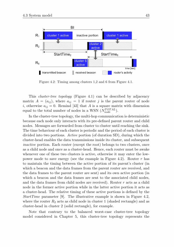
4.3 System model 43
Figure 4.2: Timing among clusters 1,2 and 6 from Figure 4.1.
This cluster-tree topology (Figure 4.1) can be described by adjacencymatrix A = (aij), where aij = 1 if router j is the parent router of nodei, otherwise aij = 0. Remind [43] that A is a square matrix with dimensionequal to the total number of nodes in a WSN (NTOTAL
node ).In the cluster-tree topology, the multi-hop communication is deterministic
because each node only interacts with its pre-defined parent router and childnodes. Messages are forwarded from cluster to cluster until reaching the sink.The time behaviour of each cluster is periodic and the period of each cluster isdivided into two portions. Active portion (of duration SD), during which thecluster-head enables the data transmissions inside its cluster, and subsequentinactive portion. Each router (except the root) belongs to two clusters, onceas a child node and once as a cluster-head. Hence, each router must be awakewhenever one of these two clusters is active, otherwise it may enter the low-power mode to save energy (see the example in Figure 4.2). Router r hasto maintain the timing between the active portion of its parent’s cluster (inwhich a beacon and the data frames from the parent router are received, andthe data frames to the parent router are sent) and its own active portion (inwhich a beacon and the data frames are sent to the associated child nodes,and the data frames from child nodes are received). Router r acts as a childnode in the former active portion while in the latter active portion it acts asa cluster-head. The relative timing of these active portions is defined by theStartTime parameter [9]. The illustrative example is shown in Figure 4.2,where the router R2 acts as child node in cluster 1 (shaded rectangle) and ascluster-head in cluster 2 (solid rectangle), for example.
Note that contrary to the balanced worst-case cluster-tree topologymodel considered in Chapter 5, this cluster-tree topology represents the
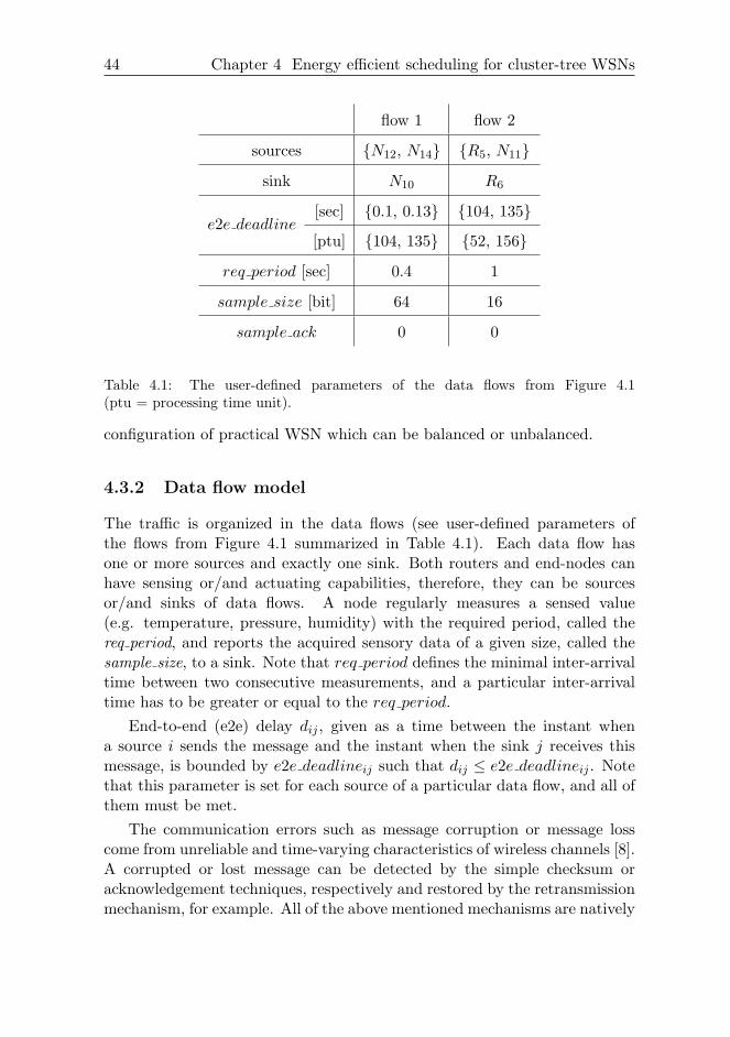
44 Chapter 4 Energy efficient scheduling for cluster-tree WSNs
flow 1 flow 2
sources N12, N14 R5, N11
sink N10 R6
e2e deadline[sec] 0.1, 0.13 104, 135
[ptu] 104, 135 52, 156
req period [sec] 0.4 1
sample size [bit] 64 16
sample ack 0 0
Table 4.1: The user-defined parameters of the data flows from Figure 4.1(ptu = processing time unit).
configuration of practical WSN which can be balanced or unbalanced.
4.3.2 Data flow model
The traffic is organized in the data flows (see user-defined parameters ofthe flows from Figure 4.1 summarized in Table 4.1). Each data flow hasone or more sources and exactly one sink. Both routers and end-nodes canhave sensing or/and actuating capabilities, therefore, they can be sourcesor/and sinks of data flows. A node regularly measures a sensed value(e.g. temperature, pressure, humidity) with the required period, called thereq period, and reports the acquired sensory data of a given size, called thesample size, to a sink. Note that req period defines the minimal inter-arrivaltime between two consecutive measurements, and a particular inter-arrivaltime has to be greater or equal to the req period.
End-to-end (e2e) delay dij , given as a time between the instant whena source i sends the message and the instant when the sink j receives thismessage, is bounded by e2e deadlineij such that dij ≤ e2e deadlineij . Notethat this parameter is set for each source of a particular data flow, and all ofthem must be met.
The communication errors such as message corruption or message losscome from unreliable and time-varying characteristics of wireless channels [8].A corrupted or lost message can be detected by the simple checksum oracknowledgement techniques, respectively and restored by the retransmissionmechanism, for example. All of the above mentioned mechanisms are natively

4.3 System model 45
supported by the IEEE 802.15.4 protocol [9]. The messages of a givendata flow can be transmitted without acknowledgement, i.e. parametersample ack = 0, or with acknowledgement, i.e. sample ack = 1. Notethat the maximum number of retransmissions must be bounded, otherwise,the analysis will not be possible.
The length of active portion, and consequently the length of schedule,grows with the maximum number of retransmissions. Given a channel errorrate, the simulation study is used to show interdependence of timeliness,energy consumption and reliability, in a way that improving one may degradethe others (Section 4.6).
4.3.3 Cyclic nature
In cluster-tree WSNs, the flows traverse different clusters on their routingpaths from the source nodes to the sink nodes. One execution of the flow(i.e. complete data communication from the source node/nodes to the sinknode) is called a wave, and the notation fk
i is used to denote wave k ofthe flow i. The flows are assumed to be transmitted with the same period,therefore wave fk
i is followed by wave fk+1i for all flows and all waves with the
same time separation. The cluster is active only once during the period [10],therefore all the flows in a given cluster are bound together. For example, thegray rectangles on the first line of Figure 4.3 show active portions of cluster 1during three consecutive periods accommodating flows 1 and 2 in each period.The key problem is to find a periodic schedule, called Time Division ClusterSchedule (TDCS), which specifies when the clusters are active while avoidingpossible inter-cluster collisions and meeting all data flows’ e2e deadlines. Theschedule is characterized not only by the moments when the clusters becomeactive within the period, but due to the cyclic nature of the problem it isalso characterized by the index of the wave for each flow in a given cluster.
Figure 4.3 shows two possible schedules of the example in Figure 4.1. Evenif we relax on the lengths of transmitted messages and on resource constraintsrelated to the cluster collisions, we have to deal with the precedence relationsof the wave traversing different clusters. Since the flows have oppositedirections in this example, the e2e delay minimization of the first flow isin contradiction with the the minimization of the second flow. Figure 4.3ashows the case, when e2e delay of the flow 1 is minimized, i.e. the orderedsequence of clusters’ active portions is in line with the flow 1 (starting withclusters 4 and 6 and following with clusters 2, 1 and 3), and therefore onewave of this flow fits into one period. On the other hand, the wave of theflow 2 spans over 3 periods while going against the sequence of clusters.
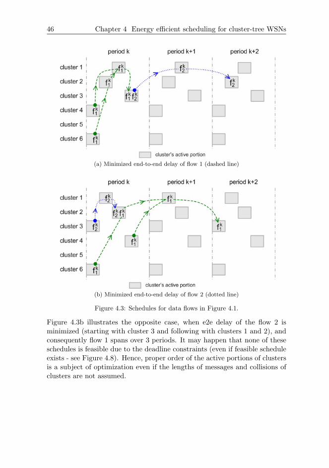
46 Chapter 4 Energy efficient scheduling for cluster-tree WSNs
(a) Minimized end-to-end delay of flow 1 (dashed line)
(b) Minimized end-to-end delay of flow 2 (dotted line)
Figure 4.3: Schedules for data flows in Figure 4.1.
Figure 4.3b illustrates the opposite case, when e2e delay of the flow 2 isminimized (starting with cluster 3 and following with clusters 1 and 2), andconsequently flow 1 spans over 3 periods. It may happen that none of theseschedules is feasible due to the deadline constraints (even if feasible scheduleexists - see Figure 4.8). Hence, proper order of the active portions of clustersis a subject of optimization even if the lengths of messages and collisions ofclusters are not assumed.
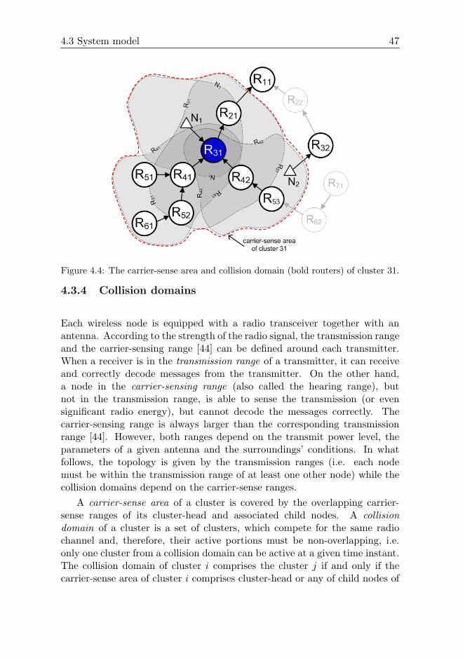
4.3 System model 47
Figure 4.4: The carrier-sense area and collision domain (bold routers) of cluster 31.
4.3.4 Collision domains
Each wireless node is equipped with a radio transceiver together with anantenna. According to the strength of the radio signal, the transmission rangeand the carrier-sensing range [44] can be defined around each transmitter.When a receiver is in the transmission range of a transmitter, it can receiveand correctly decode messages from the transmitter. On the other hand,a node in the carrier-sensing range (also called the hearing range), butnot in the transmission range, is able to sense the transmission (or evensignificant radio energy), but cannot decode the messages correctly. Thecarrier-sensing range is always larger than the corresponding transmissionrange [44]. However, both ranges depend on the transmit power level, theparameters of a given antenna and the surroundings’ conditions. In whatfollows, the topology is given by the transmission ranges (i.e. each nodemust be within the transmission range of at least one other node) while thecollision domains depend on the carrier-sense ranges.
A carrier-sense area of a cluster is covered by the overlapping carrier-sense ranges of its cluster-head and associated child nodes. A collisiondomain of a cluster is a set of clusters, which compete for the same radiochannel and, therefore, their active portions must be non-overlapping, i.e.only one cluster from a collision domain can be active at a given time instant.The collision domain of cluster i comprises the cluster j if and only if thecarrier-sense area of cluster i comprises cluster-head or any of child nodes of
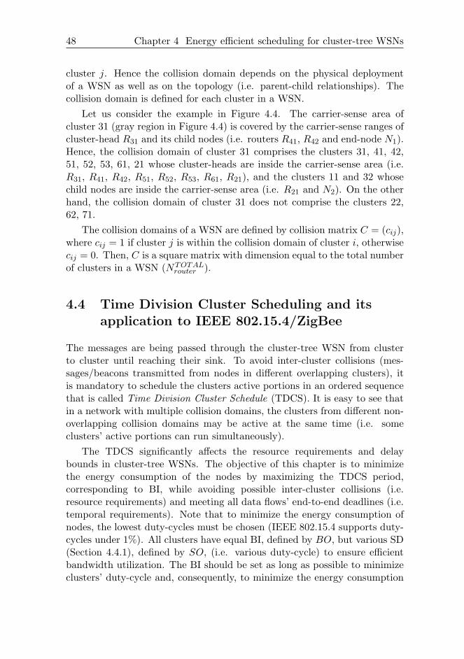
48 Chapter 4 Energy efficient scheduling for cluster-tree WSNs
cluster j. Hence the collision domain depends on the physical deploymentof a WSN as well as on the topology (i.e. parent-child relationships). Thecollision domain is defined for each cluster in a WSN.
Let us consider the example in Figure 4.4. The carrier-sense area ofcluster 31 (gray region in Figure 4.4) is covered by the carrier-sense ranges ofcluster-head R31 and its child nodes (i.e. routers R41, R42 and end-node N1).Hence, the collision domain of cluster 31 comprises the clusters 31, 41, 42,51, 52, 53, 61, 21 whose cluster-heads are inside the carrier-sense area (i.e.R31, R41, R42, R51, R52, R53, R61, R21), and the clusters 11 and 32 whosechild nodes are inside the carrier-sense area (i.e. R21 and N2). On the otherhand, the collision domain of cluster 31 does not comprise the clusters 22,62, 71.
The collision domains of a WSN are defined by collision matrix C = (cij),where cij = 1 if cluster j is within the collision domain of cluster i, otherwisecij = 0. Then, C is a square matrix with dimension equal to the total numberof clusters in a WSN (NTOTAL
router ).
4.4 Time Division Cluster Scheduling and itsapplication to IEEE 802.15.4/ZigBee
The messages are being passed through the cluster-tree WSN from clusterto cluster until reaching their sink. To avoid inter-cluster collisions (mes-sages/beacons transmitted from nodes in different overlapping clusters), itis mandatory to schedule the clusters active portions in an ordered sequencethat is called Time Division Cluster Schedule (TDCS). It is easy to see thatin a network with multiple collision domains, the clusters from different non-overlapping collision domains may be active at the same time (i.e. someclusters’ active portions can run simultaneously).
The TDCS significantly affects the resource requirements and delaybounds in cluster-tree WSNs. The objective of this chapter is to minimizethe energy consumption of the nodes by maximizing the TDCS period,corresponding to BI, while avoiding possible inter-cluster collisions (i.e.resource requirements) and meeting all data flows’ end-to-end deadlines (i.e.temporal requirements). Note that to minimize the energy consumption ofnodes, the lowest duty-cycles must be chosen (IEEE 802.15.4 supports duty-cycles under 1%). All clusters have equal BI, defined by BO, but various SD(Section 4.4.1), defined by SO, (i.e. various duty-cycle) to ensure efficientbandwidth utilization. The BI should be set as long as possible to minimizeclusters’ duty-cycle and, consequently, to minimize the energy consumption
4.4 Time Division Cluster Scheduling 49
of the nodes. As a result, the clusters inactive portion is extended, andthe nodes may stay in the low power mode longer to save energy. On theother hand, minimum duty-cycles enlarge the end-to-end delays. Hence, longlifetime is in contrast to the fast timing response of a WSN, therefore theinterest in in finding the TDCS minimazing the duty-cycles while respectingall of the required data flows e2e deadlines.
The key idea of this chapter is to formulate the problem of finding afeasible TDCS as a cyclic extension of the RCPS/TC (Resource ConstrainedProject Scheduling with Temporal Constraints) problem [45], so that theusers are not restricted to a particular implementation but they can make asimilar extension to any of the algorithms solving this problem.
The TDCS algorithm (formulated in Sections 4.4.2, 4.4.3 and solved inSection 4.4.4) is called iteratively starting from the minimum BI up to themaximum BI. The maximum BI, given by BOmax in Eq.(2.1), is equal toor shorter than the shortest req period among all of the data flows. Theminimum BI, given by BOmin, is equal to or longer than the duration ofall clusters’ SDs when assuming that non-interfering clusters overlap. If afeasible TDCS is found for a given BI, BO is increased by 1 and the TDCSalgorithm is called once again with new BI. This procedure is repeated untilBO = BOmax or a feasible TDCS is not found. Then, the last feasibleTDCS meets all the resource and temporal requirements while minimizingthe energy consumption of the nodes.
4.4.1 Duration of the cluster’s active portion inIEEE 802.15.4/ZigBee
The duration of the cluster’s active portion (SD) is given by the amountof data traffic traversed through a given cluster. To reduce the resourcerequirements of the routers and end-to-end delays, the following priorityrule is introduced: ”When a cluster-head handles several GTSs in oppositedirections, the transmit GTSs (i.e. communication from child-node to cluster-head) are allocated before the receive GTSs (i.e. communication from cluster-head to child-node)”. Using this rule, the end-to-end delay of a flow can bereduced by one period of TDCS at a router which allocates both receiveand transmit GTSs for a given flow. For example, in Figure 4.1, routerR1 allocates one transmit GTSs and one receive GTS for flow 1. In order toreduce the computational complexity, the GTSs inside the transmit or receivegroup are in an arbitrary order and are not the subject of the optimization.
The length of each GTS is given by the amount of transmitted data.Each GTS includes effective data transmission and overheads (i.e. inter-
50 Chapter 4 Energy efficient scheduling for cluster-tree WSNs
frame spacing (IFS) and eventual acknowledgement and retransmissions -see Section 2.3). The whole transmission, including the data frame, IFS andeventual acknowledgement and retransmissions, must be completed beforethe end of the current GTS. Otherwise, it must wait until the GTS in thenext superframe.
The duration of a GTS required for the whole data transmission isexpressed as:
TGTS =
e∑i=1
∆IFSi + (macMaxFrameRetries · sample acki + 1)·
(frm sizei/rate+macAckWaitDuration · sample acki)
(4.1)
where frm size is the size of transmitted frame including the data payload,MAC and PHY headers; rate is the data rate equal to 250 kbps; ∆IFS isequal to SIFS or LIFS depending on the length of MAC frame; and e is thenumber of flows in the transmit or receive direction belonging to a given childnode.
The number of allocated time slots for a given GTS is then equal to:
NGTS =⌈TGTS
TS
⌉(4.2)
where TS is the duration of a time slot and is equal to SD/16. The number oftime slots, NGTS , is calculated for each allocated GTS in a given superframe.The remaining time slots of SD are utilized for the best-effort traffic withinthe CAP. The allocated GTSs cannot reduce the length of the CAP to lessthan aMinCAPLength [9].
The superframe duration (SD) is then computed iteratively starting fromSO = 0. If the number of time slots required for all allocated GTSs in agiven superframe is greater than 16 − daMinCAPLength/TSe, the SO isincreased by 1 and the length of each GTS (Eq. (4.2)) is recalculated. Thisprocedure is repeated until all allocated GTSs fit into a given SD.
To ensure efficient bandwidth utilization, the SD of the clusters handlinga higher amount of data traffic should be longer than the ones handling lessamount of data traffic. Thus, the adequate SD is computed for each clustersuch that for each cluster k, we get SOk and the configuration parameters [9]of each allocated GTS, i.e. GTS device, GTS direction, GTS length andGTS starting slot. In case of the example in Figure 4.1, the configurationparameters are summarized in Table 4.2. Note that all clusters have the same
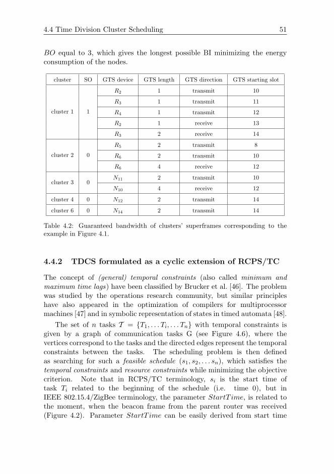
4.4 Time Division Cluster Scheduling 51
BO equal to 3, which gives the longest possible BI minimizing the energyconsumption of the nodes.
cluster SO GTS device GTS length GTS direction GTS starting slot
cluster 1 1
R2 1 transmit 10
R3 1 transmit 11
R4 1 transmit 12
R2 1 receive 13
R3 2 receive 14
cluster 2 0
R5 2 transmit 8
R6 2 transmit 10
R6 4 receive 12
cluster 3 0N11 2 transmit 10
N10 4 receive 12
cluster 4 0 N12 2 transmit 14
cluster 6 0 N14 2 transmit 14
Table 4.2: Guaranteed bandwidth of clusters’ superframes corresponding to theexample in Figure 4.1.
4.4.2 TDCS formulated as a cyclic extension of RCPS/TC
The concept of (general) temporal constraints (also called minimum andmaximum time lags) have been classified by Brucker et al. [46]. The problemwas studied by the operations research community, but similar principleshave also appeared in the optimization of compilers for multiprocessormachines [47] and in symbolic representation of states in timed automata [48].
The set of n tasks T = T1, . . . Ti, . . . Tn with temporal constraints isgiven by a graph of communication tasks G (see Figure 4.6), where thevertices correspond to the tasks and the directed edges represent the temporalconstraints between the tasks. The scheduling problem is then definedas searching for such a feasible schedule (s1, s2, . . . sn), which satisfies thetemporal constraints and resource constraints while minimizing the objectivecriterion. Note that in RCPS/TC terminology, si is the start time oftask Ti related to the beginning of the schedule (i.e. time 0), but inIEEE 802.15.4/ZigBee terminology, the parameter StartT ime, is related tothe moment, when the beacon frame from the parent router was received(Figure 4.2). Parameter StartT ime can be easily derived from start time
52 Chapter 4 Energy efficient scheduling for cluster-tree WSNs
s and matrix A, since parameter StartT ime of the root is equal to 0 (seeEq. (4.12) for more details).
Each edge from vertex Ti to vertex Tj is labelled by a weight wi,j whichconstraints the start times of the tasks Ti and Tj by the inequality sj − si ≥wi,j . There are two kinds of edges: the edges with positive weights and theedges with negative weights. The edge, from vertex Ti to vertex Tj with apositive weight wi,j (giving the minimum time lag), indicates that sj , thestart time of Tj , must be at least wi,j time units after si, the start time ofTi (i.e. sj ≥ si + wi,j). We use the positive weights wi,j to represent theprecedence constraint, i.e. wi,j = pi and therefore Tj starts after completionof Ti, where pi is processing time of Ti.
The edge, from vertex Tj to vertex Ti with a negative weight wj,i (givingthe maximum time lag), indicates that sj must be no more than |wj,i| timeunits after si (i.e. sj ≤ si + wj,i). Therefore, each negative weight wj,i
represents the relative deadline of task Tj in relation to task Ti. Consequently,when Tj is the last task of the flow and Ti is the first task of the same flow,the edge with a negative weight may be conveniently applied for e2e deadlinesuch that the value of e2e deadline is equal to |wj,i|+ pj .
Any feasible TDCS has to respect the resource constraints related to thecollision domains of clusters and the temporal constraints of the flows. Hence,the set of tasks T will consist of two disjoint subsets: a set of cluster-tasks anda set of dummy-tasks reflecting the temporal constraints only. The durationof a task Ti is given by its processing time pi.
The cluster-task Ti is created for each cluster i. Note that the clusterswhich do not route any data flow have pi = 0 (i.e. cluster-task 5 is not shownin Figure 4.6). In the case of an active cluster-task (i.e. the one routingat least one data flow) the processing time is equal to the cluster’s SD (i.e.pi = SD computed in Section 4.4.1) and includes all the communicationshandled by the given cluster. That means, for each cluster-task, we definethe duration of the CAP as pCAP
i , the duration of all GTSs in the transmitdirection as pT
i and the duration of all GTSs in the receive direction as pRi ,
i.e. the processing time of cluster-task is given as pi = pCAPi + pT
i + pRi . The
unit of processing time, called ptu, is equal to the length of a time slot whenSO = 0 (i.e. 1 ptu = aBaseSuperframeDuration/16 = 0.96 ms).
Each dummy-task has a processing time equal to 0 since they are used tohandle temporal constraints of different flows.
Let us consider the illustrative example of cluster-tree WSN in Figure 4.1,where periodic time-bounded traffic is sent using two data flows. Within thefirst data flow, messages are sent from source nodes N12 and N14 to the
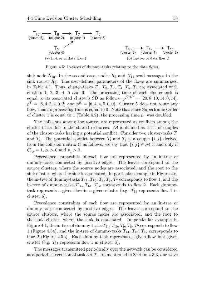
4.4 Time Division Cluster Scheduling 53
(a) In-tree of data flow 1. (b) In-tree of data flow 2.
Figure 4.5: In-trees of dummy-tasks relating to the data flows.
sink node N10. In the second case, nodes R5 and N11 send messages to thesink router R6. The user-defined parameters of the flows are summarizedin Table 4.1. Thus, cluster-tasks T1, T2, T3, T4, T5, T6 are associated withclusters 1, 2, 3, 4, 5 and 6. The processing time of each cluster-task isequal to its associated cluster’s SD as follows: pCAP = [20, 8, 10, 14, 0, 14],pT = [6, 4, 2, 2, 0, 2] and pR = [6, 4, 4, 0, 0, 0]. Cluster 5 does not route anyflow, thus its processing time is equal to 0. Note that since Superframe Orderof cluster 1 is equal to 1 (Table 4.2), the processing time p1 was doubled.
The collisions among the routers are represented as conflicts among thecluster-tasks due to the shared resources. M is defined as a set of couplesof the cluster-tasks having a potential conflict. Consider two cluster-tasks Ti
and Tj . The potential conflict between Ti and Tj is a couple i, j derivedfrom the collision matrix C as follows: we say that i, j ∈ M if and only ifCi,j = 1, pi > 0 and pj > 0.
Precedence constraints of each flow are represented by an in-tree ofdummy-tasks connected by positive edges. The leaves correspond to thesource clusters, where the source nodes are associated, and the root to thesink cluster, where the sink is associated. In particular example in Figure 4.6,the in-tree of dummy-tasks T11, T10, T9, T8, T7 corresponds to flow 1, and thein-tree of dummy-tasks T14, T13, T12 corresponds to flow 2. Each dummy-task represents a given flow in a given cluster (e.g. T11 represents flow 1 incluster 6).
Precedence constraints of each flow are represented by an in-tree ofdummy-tasks connected by positive edges. The leaves correspond to thesource clusters, where the source nodes are associated, and the root tothe sink cluster, where the sink is associated. In particular example inFigure 4.1, the in-tree of dummy-tasks T11, T10, T9, T8, T7 corresponds to flow1 (Figure 4.5a), and the in-tree of dummy-tasks T14, T13, T12 corresponds toflow 2 (Figure 4.5b). Each dummy-task represents a given flow in a givencluster (e.g. T11 represents flow 1 in cluster 6).
The messages transmitted periodically over the network can be consideredas a periodic execution of task-set T . As mentioned in Section 4.3.3, one wave
54 Chapter 4 Energy efficient scheduling for cluster-tree WSNs
of a given flow may go over several periods and, therefore, we are faced witha cyclic scheduling problem.
Let si be the start time within the period, i.e. remainder after divisionof si by BI, and let qi be the index of the period, i.e. the integer part of thisdivision. Then start time si can be expressed as follows:
si = si + qi · BI for si ∈ 〈0,BI− 1〉 , qi ≥ 0. (4.3)
This notation divides si into segment qi and offset si. Hence, two tasks Ti
and Tj within one period may have a different qi and qj , since the pieces ofdata related to these tasks correspond to the different waves (this notion usedin cyclic scheduling is identical to the modulo scheduling or SW pipeliningin the parallel compiler community [49]).
The cyclic schedule has to follow several constraints:
– Precedence constraints and relative deadlines are given by inequalitysj − si ≥ wi,j . As a result, by applying Eq. (4.3) we obtain:
(sj + qj · BI)− (si + qi · BI) ≥ wi,j . (4.4)
– Offset precedence constraints and offset relative deadlines are usedto bind the flow-related dummy tasks with the cluster-task. Theyrepresent the relation between two tasks that can be from differentwaves. Therefore, they do not contain the segment values q and can beexpressed as:
sj − si ≥ vi,j . (4.5)
The offset weights vi,j are used to distinguish the offset precedenceconstraints from ”normal” precedence constraints.
– Resource constraints given by M, the set of potential conflicts of thecluster-tasks. The conflicts have to be avoided in order to obtain afeasible schedule (detailed explanation is given in Section 4.4.4).
4.4.3 Graph of the communication tasks
An important step of the scheduling algorithm is the construction of thegraph of the communication tasks G (Figure 4.6) using the data flows inTable 4.1 and topology in Figure 4.1 (i.e. adjacency matrix A and collisionmatrix C).
Each dummy-task is synchronized with the corresponding cluster-task.The synchronization is made by means of offset precedence constraints
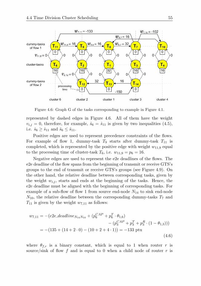
4.4 Time Division Cluster Scheduling 55
Figure 4.6: Graph G of the tasks corresponding to example in Figure 4.1.
represented by dashed edges in Figure 4.6. All of them have the weightvi,j = 0, therefore, for example, s6 = s11 is given by two inequalities (4.5),i.e. s6 ≥ s11 and s6 ≤ s11.
Positive edges are used to represent precedence constraints of the flows.For example of flow 1, dummy-task T9 starts after dummy-task T11 iscompleted, which is represented by the positive edge with weight w11,9 equalto the processing time of cluster-task T6, i.e. w11,9 = p6 = 16.
Negative edges are used to represent the e2e deadlines of the flows. Thee2e deadline of the flow spans from the beginning of transmit or receive GTS’sgroups to the end of transmit or receive GTS’s groups (see Figure 4.9). Onthe other hand, the relative deadline between corresponding tasks, given bythe weight wi,j , starts and ends at the beginning of the tasks. Hence, thee2e deadline must be aligned with the beginning of corresponding tasks. Forexample of a sub-flow of flow 1 from source end-node N14 to sink end-nodeN10, the relative deadline between the corresponding dummy-tasks T7 andT11 is given by the weight w7,11 as follows:
w7,11 = −(e2e deadlineN14N10 + (pCAP
6 + pT6 · θ1,6)
− (pCAP3 + pT
3 + pR3 · (1− θ1,3))
)= −
(135 + (14 + 2 · 0)− (10 + 2 + 4 · 1)
)= −133 ptu
(4.6)
where θf,r is a binary constant, which is equal to 1 when router r issource/sink of flow f and is equal to 0 when a child node of router r is
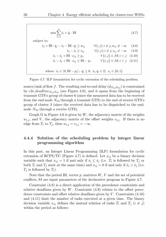
56 Chapter 4 Energy efficient scheduling for cluster-tree WSNs
minn∑
i=1
si + qi · BI (4.7)
subject to:sj + BI · qj − si − BI · qi ≥ wij ∀(i, j); i 6= j, wij 6= −∞ (4.8)
sj − si ≥ vij ∀(i, j); i 6= j, vij 6= −∞ (4.9)si − sj + BI · xij ≥ pj ∀ i, j ∈ M; i < j (4.10)si − sj + BI · xij ≤ BI− pi ∀ i, j ∈ M; i < j (4.11)
where: si ∈ 〈0,BI− pi〉 ; qi ≥ 0; si, qi ∈ Z; xi ∈ 0, 1
Figure 4.7: ILP formulation for cyclic extension of the scheduling problem.
source/sink of flow f . The resulting end-to-end delay (dN14N10) is constrainedby e2e deadlineN14N10 (see Figure 4.9), and it spans from the beginning oftransmit GTS’s group of cluster 6 (since the measured data has to be receivedfrom the end-node N14 through a transmit GTS) to the end of receive GTS’sgroup of cluster 3 (since the received data has to be dispatched to the end-node N10 through a receive GTS).
Graph G in Figure 4.6 is given by W , the adjacency matrix of the weightswi,j , and V , the adjacency matrix of the offset weights vi,j . If there is noedge from Ti to Tj , then wi,j = vi,j = −∞.
4.4.4 Solution of the scheduling problem by integer linearprogramming algorithm
In this part, an Integer Linear Programming (ILP) formulation for cyclicextension of RCPS/TC (Figure 4.7) is defined. Let xij be a binary decisionvariable such that xij = 1 if and only if si ≤ sj (i.e. Ti is followed by Tj orboth Ti and Tj start at the same time) and xij = 0 if and only if si > sj (i.e.Tj is followed by Ti).
Note that the period BI, vector p, matrices W , V and the set of potentialconflicts M are input parameters of the declarative program in Figure 4.7.
Constraint (4.8) is a direct application of the precedence constraints andrelative deadlines given by W . Constraint (4.9) relates to the offset prece-dence constraints and offset relative deadlines given by V . Constraints (4.10)and (4.11) limit the number of tasks executed at a given time. The binarydecision variable xij defines the mutual relation of tasks Ti and Tj (i 6= j)within the period as follows:
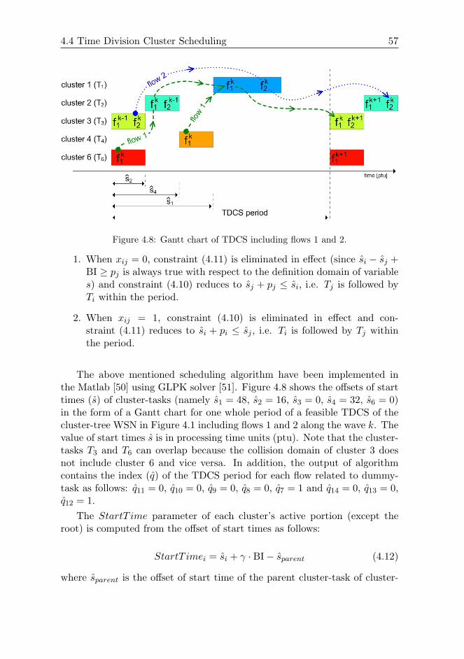
4.4 Time Division Cluster Scheduling 57
Figure 4.8: Gantt chart of TDCS including flows 1 and 2.
1. When xij = 0, constraint (4.11) is eliminated in effect (since si − sj +BI ≥ pj is always true with respect to the definition domain of variables) and constraint (4.10) reduces to sj + pj ≤ si, i.e. Tj is followed byTi within the period.
2. When xij = 1, constraint (4.10) is eliminated in effect and con-straint (4.11) reduces to si + pi ≤ sj , i.e. Ti is followed by Tj withinthe period.
The above mentioned scheduling algorithm have been implemented inthe Matlab [50] using GLPK solver [51]. Figure 4.8 shows the offsets of starttimes (s) of cluster-tasks (namely s1 = 48, s2 = 16, s3 = 0, s4 = 32, s6 = 0)in the form of a Gantt chart for one whole period of a feasible TDCS of thecluster-tree WSN in Figure 4.1 including flows 1 and 2 along the wave k. Thevalue of start times s is in processing time units (ptu). Note that the cluster-tasks T3 and T6 can overlap because the collision domain of cluster 3 doesnot include cluster 6 and vice versa. In addition, the output of algorithmcontains the index (q) of the TDCS period for each flow related to dummy-task as follows: q11 = 0, q10 = 0, q9 = 0, q8 = 0, q7 = 1 and q14 = 0, q13 = 0,q12 = 1.
The StartT ime parameter of each cluster’s active portion (except theroot) is computed from the offset of start times as follows:
StartT imei = si + γ · BI− sparent (4.12)
where sparent is the offset of start time of the parent cluster-task of cluster-
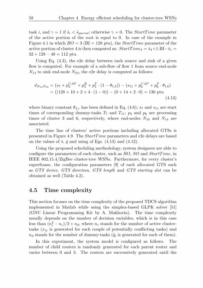
58 Chapter 4 Energy efficient scheduling for cluster-tree WSNs
task i, and γ = 1 if si < sparent; otherwise γ = 0. The StartT ime parameterof the active portion of the root is equal to 0. In case of the example inFigure 4.1 in which BO = 3 (BI = 128 ptu), the StartT ime parameter of theactive portion of cluster 4 is then computed as: StartT ime4 = s4+1·BI−s1 =32 + 128− 48 = 112 ptu.
Using Eq. (4.3), the e2e delay between each source and sink of a givenflow is computed. For example of a sub-flow of flow 1 from source end-nodeN14 to sink end-node N10, the e2e delay is computed as follows:
dN14N10 =(s7 + pCAP
3 + pR3 + pT
3 · (1− θ1,3))−(s11 + pCAP
6 + pT6 · θ1,6
)=((128 + 10 + 2 + 4 · (1− 0)
)−(0 + 14 + 2 · 0
)= 130 ptu
(4.13)
where binary constant θf,r has been defined in Eq. (4.6); s7 and s11 are starttimes of corresponding dummy-tasks T7 and T11; p3 and p6 are processingtimes of cluster 3 and 6, respectively, where end-nodes N10 and N14 areassociated.
The time line of clusters’ active portions including allocated GTSs ispresented in Figure 4.9. The StartT ime parameters and e2e delays are basedon the values of s, q and using of Egs. (4.13) and (4.12).
Using the proposed scheduling methodology, system designers are able toconfigure the parameters of each cluster, such as BO, SO and StartT ime, inIEEE 802.15.4/ZigBee cluster-tree WSNs. Furthermore, for every cluster’ssuperframe, the configuration parameters [9] of each allocated GTS suchas GTS device, GTS direction, GTS length and GTS starting slot can beobtained as well (Table 4.2).
4.5 Time complexity
This section focuses on the time complexity of the proposed TDCS algorithmimplemented in Matlab while using the simplex-based GLPK solver [51](GNU Linear Programming Kit by A. Makhorin). The time complexityusually depends on the number of decision variables, which is in this caseless than (n2
c − nc)/2 + nd, where nc stands for the number of active cluster-tasks (xij is generated for each couple of potentially conflicting tasks) andnd stands for the number of dummy-tasks (qi is generated for each of them).
In this experiment, the system model is configured as follows. Thenumber of child routers is randomly generated for each parent router andvaries between 0 and 3. The routers are successively generated until the
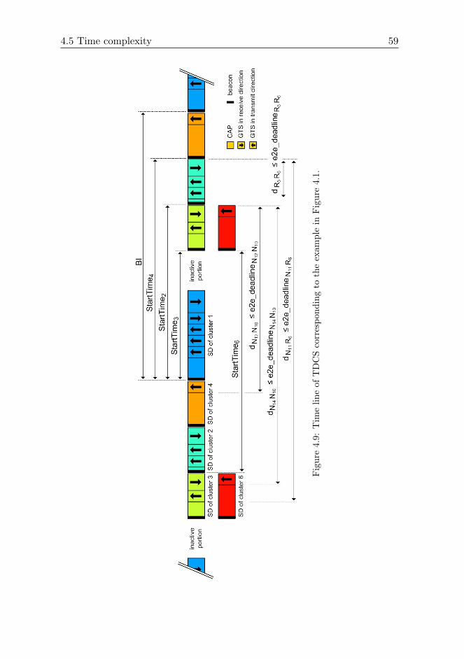
4.5 Time complexity 59
Fig
ure
4.9:
Tim
elin
eof
TD
CS
corr
espo
ndin
gto
the
exam
ple
inF
igur
e4.
1.
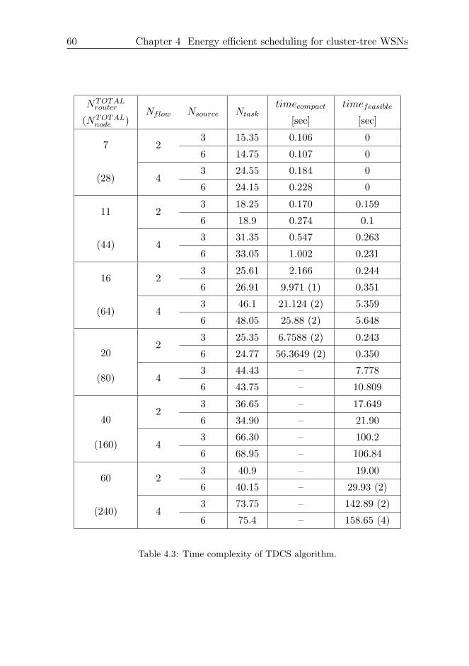
60 Chapter 4 Energy efficient scheduling for cluster-tree WSNs
NTOTALrouter Nflow Nsource Ntask
timecompact timefeasible
(NTOTALnode ) [sec] [sec]
7 23 15.35 0.106 0
6 14.75 0.107 0
(28) 43 24.55 0.184 0
6 24.15 0.228 0
11 23 18.25 0.170 0.159
6 18.9 0.274 0.1
(44) 43 31.35 0.547 0.263
6 33.05 1.002 0.231
16 23 25.61 2.166 0.244
6 26.91 9.971 (1) 0.351
(64) 43 46.1 21.124 (2) 5.359
6 48.05 25.88 (2) 5.648
202
3 25.35 6.7588 (2) 0.243
6 24.77 56.3649 (2) 0.350
(80) 43 44.43 – 7.778
6 43.75 – 10.809
402
3 36.65 – 17.649
6 34.90 – 21.90
(160) 43 66.30 – 100.2
6 68.95 – 106.84
60 23 40.9 – 19.00
6 40.15 – 29.93 (2)
(240) 43 73.75 – 142.89 (2)
6 75.4 – 158.65 (4)
Table 4.3: Time complexity of TDCS algorithm.
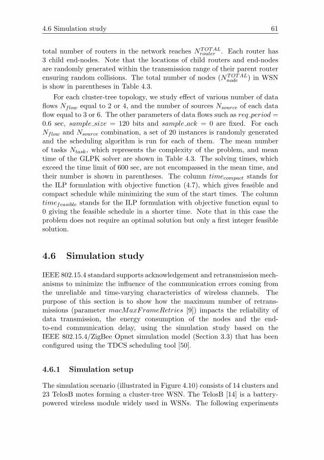
4.6 Simulation study 61
total number of routers in the network reaches NTOTALrouter . Each router has
3 child end-nodes. Note that the locations of child routers and end-nodesare randomly generated within the transmission range of their parent routerensuring random collisions. The total number of nodes (NTOTAL
node ) in WSNis show in parentheses in Table 4.3.
For each cluster-tree topology, we study effect of various number of dataflows Nflow equal to 2 or 4, and the number of sources Nsource of each dataflow equal to 3 or 6. The other parameters of data flows such as req period =0.6 sec, sample size = 120 bits and sample ack = 0 are fixed. For eachNflow and Nsource combination, a set of 20 instances is randomly generatedand the scheduling algorithm is run for each of them. The mean numberof tasks Ntask, which represents the complexity of the problem, and meantime of the GLPK solver are shown in Table 4.3. The solving times, whichexceed the time limit of 600 sec, are not encompassed in the mean time, andtheir number is shown in parentheses. The column timecompact stands forthe ILP formulation with objective function (4.7), which gives feasible andcompact schedule while minimizing the sum of the start times. The columntimefeasible stands for the ILP formulation with objective function equal to0 giving the feasible schedule in a shorter time. Note that in this case theproblem does not require an optimal solution but only a first integer feasiblesolution.
4.6 Simulation study
IEEE 802.15.4 standard supports acknowledgement and retransmission mech-anisms to minimize the influence of the communication errors coming fromthe unreliable and time-varying characteristics of wireless channels. Thepurpose of this section is to show how the maximum number of retrans-missions (parameter macMaxFrameRetries [9]) impacts the reliability ofdata transmission, the energy consumption of the nodes and the end-to-end communication delay, using the simulation study based on theIEEE 802.15.4/ZigBee Opnet simulation model (Section 3.3) that has beenconfigured using the TDCS scheduling tool [50].
4.6.1 Simulation setup
The simulation scenario (illustrated in Figure 4.10) consists of 14 clusters and23 TelosB motes forming a cluster-tree WSN. The TelosB [14] is a battery-powered wireless module widely used in WSNs. The following experiments
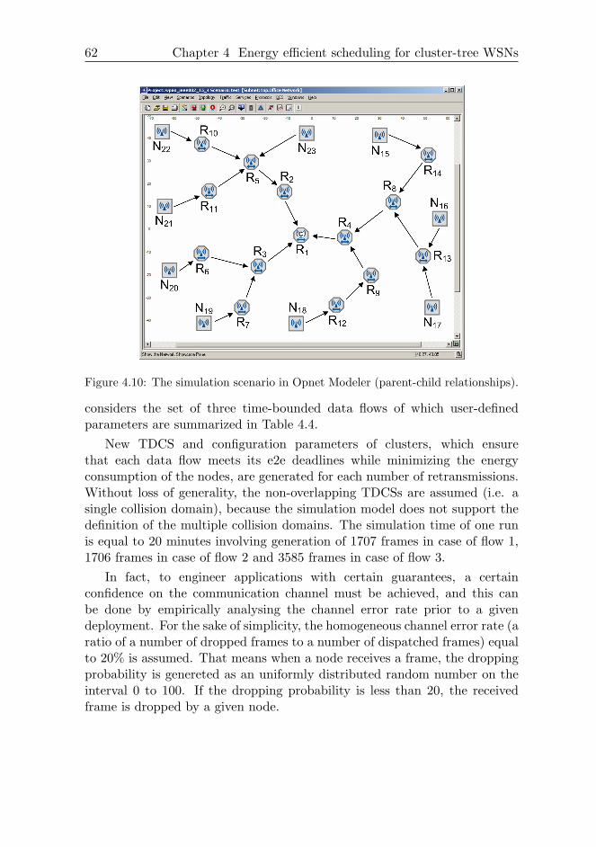
62 Chapter 4 Energy efficient scheduling for cluster-tree WSNs
Figure 4.10: The simulation scenario in Opnet Modeler (parent-child relationships).
considers the set of three time-bounded data flows of which user-definedparameters are summarized in Table 4.4.
New TDCS and configuration parameters of clusters, which ensurethat each data flow meets its e2e deadlines while minimizing the energyconsumption of the nodes, are generated for each number of retransmissions.Without loss of generality, the non-overlapping TDCSs are assumed (i.e. asingle collision domain), because the simulation model does not support thedefinition of the multiple collision domains. The simulation time of one runis equal to 20 minutes involving generation of 1707 frames in case of flow 1,1706 frames in case of flow 2 and 3585 frames in case of flow 3.
In fact, to engineer applications with certain guarantees, a certainconfidence on the communication channel must be achieved, and this canbe done by empirically analysing the channel error rate prior to a givendeployment. For the sake of simplicity, the homogeneous channel error rate (aratio of a number of dropped frames to a number of dispatched frames) equalto 20% is assumed. That means when a node receives a frame, the droppingprobability is genereted as an uniformly distributed random number on theinterval 0 to 100. If the dropping probability is less than 20, the receivedframe is dropped by a given node.
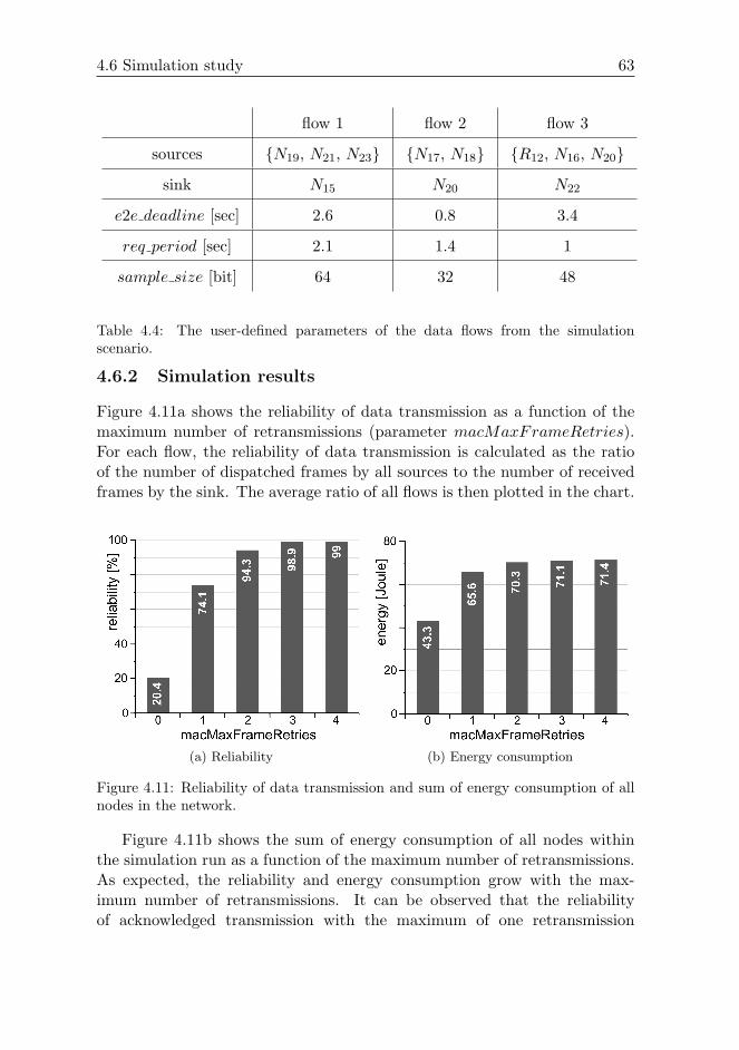
4.6 Simulation study 63
flow 1 flow 2 flow 3
sources N19, N21, N23 N17, N18 R12, N16, N20
sink N15 N20 N22
e2e deadline [sec] 2.6 0.8 3.4
req period [sec] 2.1 1.4 1
sample size [bit] 64 32 48
Table 4.4: The user-defined parameters of the data flows from the simulationscenario.
4.6.2 Simulation results
Figure 4.11a shows the reliability of data transmission as a function of themaximum number of retransmissions (parameter macMaxFrameRetries).For each flow, the reliability of data transmission is calculated as the ratioof the number of dispatched frames by all sources to the number of receivedframes by the sink. The average ratio of all flows is then plotted in the chart.
(a) Reliability (b) Energy consumption
Figure 4.11: Reliability of data transmission and sum of energy consumption of allnodes in the network.
Figure 4.11b shows the sum of energy consumption of all nodes withinthe simulation run as a function of the maximum number of retransmissions.As expected, the reliability and energy consumption grow with the max-imum number of retransmissions. It can be observed that the reliabilityof acknowledged transmission with the maximum of one retransmission
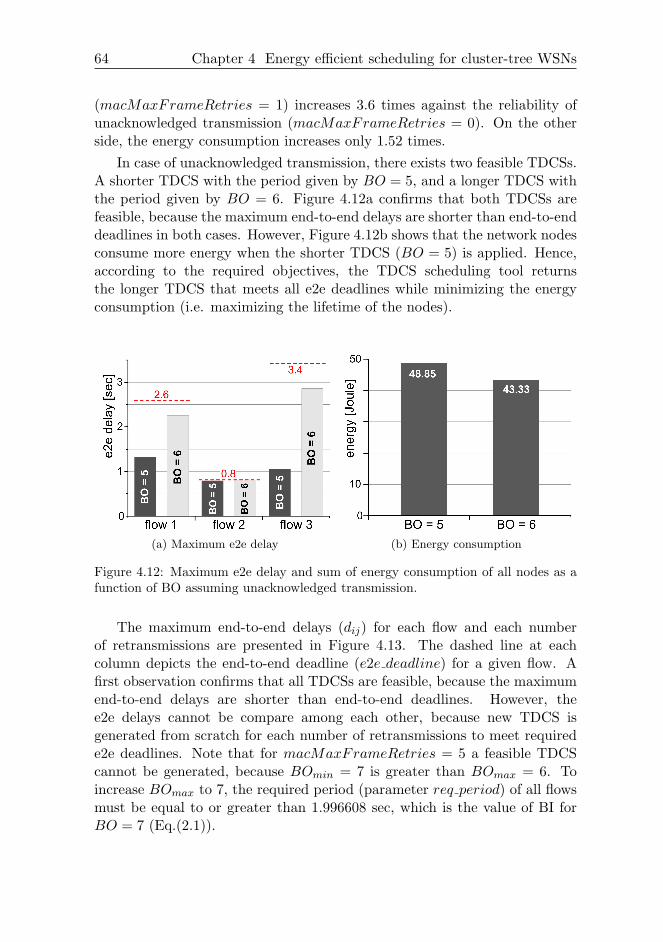
64 Chapter 4 Energy efficient scheduling for cluster-tree WSNs
(macMaxFrameRetries = 1) increases 3.6 times against the reliability ofunacknowledged transmission (macMaxFrameRetries = 0). On the otherside, the energy consumption increases only 1.52 times.
In case of unacknowledged transmission, there exists two feasible TDCSs.A shorter TDCS with the period given by BO = 5, and a longer TDCS withthe period given by BO = 6. Figure 4.12a confirms that both TDCSs arefeasible, because the maximum end-to-end delays are shorter than end-to-enddeadlines in both cases. However, Figure 4.12b shows that the network nodesconsume more energy when the shorter TDCS (BO = 5) is applied. Hence,according to the required objectives, the TDCS scheduling tool returnsthe longer TDCS that meets all e2e deadlines while minimizing the energyconsumption (i.e. maximizing the lifetime of the nodes).
(a) Maximum e2e delay (b) Energy consumption
Figure 4.12: Maximum e2e delay and sum of energy consumption of all nodes as afunction of BO assuming unacknowledged transmission.
The maximum end-to-end delays (dij) for each flow and each numberof retransmissions are presented in Figure 4.13. The dashed line at eachcolumn depicts the end-to-end deadline (e2e deadline) for a given flow. Afirst observation confirms that all TDCSs are feasible, because the maximumend-to-end delays are shorter than end-to-end deadlines. However, thee2e delays cannot be compare among each other, because new TDCS isgenerated from scratch for each number of retransmissions to meet requirede2e deadlines. Note that for macMaxFrameRetries = 5 a feasible TDCScannot be generated, because BOmin = 7 is greater than BOmax = 6. Toincrease BOmax to 7, the required period (parameter req period) of all flowsmust be equal to or greater than 1.996608 sec, which is the value of BI forBO = 7 (Eq.(2.1)).
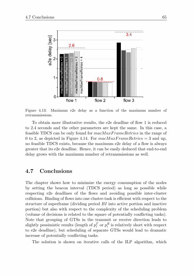
4.7 Conclusions 65
Figure 4.13: Maximum e2e delay as a function of the maximum number ofretransmissions.
To obtain more illustrative results, the e2e deadline of flow 1 is reducedto 2.4 seconds and the other parameters are kept the same. In this case, afeasible TDCS can be only found for macMaxFrameRetries in the range of0 to 2, as depicted in Figure 4.14. For macMaxFrameRetries = 3 and up,no feasible TDCS exists, because the maximum e2e delay of a flow is alwaysgreater that its e2e deadline. Hence, it can be easily deduced that end-to-enddelay grows with the maximum number of retransmissions as well.
4.7 Conclusions
The chapter shows how to minimize the energy consumption of the nodesby setting the beacon interval (TDCS period) as long as possible whilerespecting e2e deadlines of the flows and avoiding possible inter-clustercollisions. Binding of flows into one cluster-task is efficient with respect to thestructure of superframe (dividing period BI into active portion and inactiveportion) but also with respect to the complexity of the scheduling problem(volume of decisions is related to the square of potentially conflicting tasks).Note that grouping of GTSs in the transmit or receive direction leads toslightly pessimistic results (length of pT
i or pRi is relatively short with respect
to e2e deadline), but scheduling of separate GTSs would lead to dramaticincrease of potentially conflicting tasks.
The solution is shown on iterative calls of the ILP algorithm, which
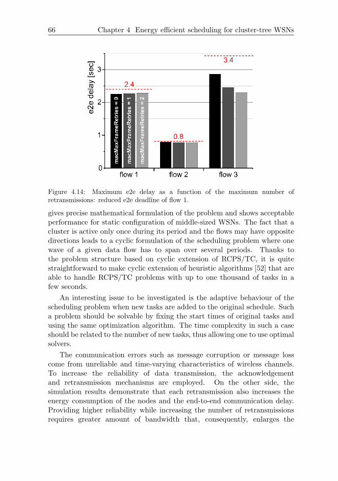
66 Chapter 4 Energy efficient scheduling for cluster-tree WSNs
Figure 4.14: Maximum e2e delay as a function of the maximum number ofretransmissions: reduced e2e deadline of flow 1.
gives precise mathematical formulation of the problem and shows acceptableperformance for static configuration of middle-sized WSNs. The fact that acluster is active only once during its period and the flows may have oppositedirections leads to a cyclic formulation of the scheduling problem where onewave of a given data flow has to span over several periods. Thanks tothe problem structure based on cyclic extension of RCPS/TC, it is quitestraightforward to make cyclic extension of heuristic algorithms [52] that areable to handle RCPS/TC problems with up to one thousand of tasks in afew seconds.
An interesting issue to be investigated is the adaptive behaviour of thescheduling problem when new tasks are added to the original schedule. Sucha problem should be solvable by fixing the start times of original tasks andusing the same optimization algorithm. The time complexity in such a caseshould be related to the number of new tasks, thus allowing one to use optimalsolvers.
The communication errors such as message corruption or message losscome from unreliable and time-varying characteristics of wireless channels.To increase the reliability of data transmission, the acknowledgementand retransmission mechanisms are employed. On the other side, thesimulation results demonstrate that each retransmission also increases theenergy consumption of the nodes and the end-to-end communication delay.Providing higher reliability while increasing the number of retransmissionsrequires greater amount of bandwidth that, consequently, enlarges the

4.7 Conclusions 67
clusters active portions. On the other side, longer active portions implyhigher duty-cycle and thus higher energy consumption of the nodes. Inaddition, longer clusters active portions may increase the TDCS period whichinduces longer end-to-end delays. Hence, the interdependence of reliability,energy consumption and timeliness make the network design more complex.
Using the proposed TDCS scheduling tool and simulation model, systemdesigners are able to configure the IEEE 802.15.4/ZigBee beacon-enabledcluster-tree WSNs and easily find the trade-off between reliability, energyconsumption and timeliness for a given application-specific implementationprior to the network deployment.

68 Chapter 4 Energy efficient scheduling for cluster-tree WSNs
APPENDIX
4.A Table of symbols
The following table reports the symbols that are used through the Chapter 4,along with their definition.
Symbol Definition
A = (aij) adjacency matrix describing parent-child tree
b total number of nodes in the WSN
C = (cij) collision matrix
G graph of communication tasks
NTOTALnode total number of nodes in a WSN
NTOTALrouter total number of routers (clusters) in a WSN
n number of tasks
pi processing time of task Ti
ptu processing time unit
qi segment of start time si
Ti task i
si start time of task Ti
si offset of start time si
vi,j offset weight
wi,j weight of the edge between tasks Ti and Tj
xij binary decision variable
Table 4.5: Table of symbols.
Chapter 5
Dimensioning and worst-caseanalysis of cluster-tree sensornetworks
5.1 Introduction
The evaluation of the performance limits of Wireless Sensor Networks(WSNs) is of paramount importance to understand their behaviour underthe worst-case conditions [53] and to make the appropriate design choices.This is particular relevant for time-sensitive WSN applications. Supportingtime-sensitive WSN applications implies to predict and guarantee boundedend-to-end communication delays. To ensure bounded end-to-end delays andto avoid buffer overflow, network resources must be known in advance, anddimensioned along the path from a source to a sink. In that direction, thischapter aims at proposing a comprehensive methodology that provides ascientific approach for quick and efficient worst-case dimensioning of networkresources (e.g. bandwidth and nodes’ buffer size) to avoid their overflowsand to minimize clusters’ duty-cycle (reducing energy consumption of thenodes) in static or even dynamically changing WSNs with a cluster-treetopology, assuming bounded communication errors. Consequently, the worst-case performance bounds (e.g. the worst-case end-to-end delay) can bederived for a cluster-tree WSN with bounded resources. The analyticalmethodology is based on Network Calculus as a trade-off between complexityand accuracy. The main benefit of using Network Calculus is its generalityand simplicity.
WSNs are commonly used for monitoring applications that gather sensory
69
70 Chapter 5 Dimensioning and worst-case analysis of cluster-tree WSNs
data in a central point called sink. In this chapter, the sink is consideredas an autonomous entity that does not make part of the WSN, butcan be associated to any of its routers through any (wired or wireless)communication means. Thus, the sink’s mobility does not impact the WSNtopology, but affects the destination of the data flows (any router in theWSN). However, while the statically associated sink is adequate for rootcentric WSN applications (e.g. an intruder alarm system delivering alerts tothe control centre), other applications may impose or benefit from collectingdata at different network locations (e.g. a doctor with a hand held computercollecting patients’ status, a fire-fighter in a rescue mission or a mobile robotin a factory-floor).
Contribution
The main outcome of this chapter is the provision of a comprehensivemethodology based on Network Calculus, which enables quick and efficientworst-case dimensioning of network resources (e.g. bandwidth and buffersize) in a static or even dynamically changing cluster-tree WSN where astatic or mobile sink gathers data from all sensor nodes. Consequently, theworst-case performance bounds (e.g. end-to-end delay) can be evaluatedfor a cluster-tree WSN with bounded resources. The designed methodologypresents two main components: (1) an analytical methodology for theworst-case dimensioning of network resources and delay bound analysis,(2) the impact of the sink’s mobility on the worst-case performance of thecluster-tree network. This enables system designers to efficiently predictnetwork resources that ensure a minimum QoS during extreme conditions(performance limits).
In particular, the Chapter 5 presents the following contributions:
1. A formulation of a simple yet efficient methodology, based on NetworkCalculus, to characterize incoming and outgoing data traffic in eachrouter in the cluster-tree WSN (Section 5.5) and to derive upper boundson buffer requirements and per-hop and end-to-end delays for bothupstream and downstream directions (Section 5.6).
2. A description of how to instantiate this methodology in the designof IEEE 802.15.4/ZigBee cluster-tree WSNs, as an illustrative examplethat confirms the applicability of general approach for specific protocols(Section 5.7).
3. A demonstration of the validity of proposed methodology throughan experimental test-bed based on Commercial-Off-The-Shelf (COTS)
5.2 Related work 71
technologies, where the experimental results are compared against thetheoretical results and assess the pessimism of the theoretical model(Section 5.8).
4. An analysis of the impact of the sink mobility on the worst-casenetwork performance and an outline of alternatives for sink mobilitymanagement, namely how routes must be updated upon the mobilityof the sink, and how this procedure affects the worst-case networkperformance (network inaccessibility times) (Section 5.9).
Notations and symbols used in this chapter are summarized in Ap-pendix 5.A.
5.2 Related work
The evaluation of the fundamental performance limits of WSNs has beenaddressed in several research works. In [53], the energy-constrained limitsof WSNs with respect to the network throughput and operational lifetimehas been evaluated. The authors have showed that with fixed node density,lifetime of WSN decreases in the order of 1/n as the number of deployed nodesn grows. Even with renewable energy sources, the maximum sustainablethroughput in energy-constrained sensor networks scales worse than thecapacity based on interference among concurrent transmissions, as long asthe physical network size grows with n in an order greater than log n.In [54], the authors have evaluated the real-time capacity of multi-hopWSNs, identifying how much real-time data the network can transfer bytheir deadlines. A capacity bound has been derived for load-balanced aswell as load-unbalanced sensor networks using (ideal) MAC protocols withfixed priority packet scheduling mechanisms. The effects of various linklayer multiplexing schemes such as time-division multiplexing and frequency-division multiplexing have been discussed. It has been shown that deadlinesare never missed when the network capacity bound is not exceeded. Bothabove mentioned papers consider ad hoc WSNs. In [55], the authors haveexplored the fundamental limits for acceptable loads, utilization and delaysin multi-hop sensor networks with fixed linear and grid topologies, in caseall sensor nodes are equally capable to reach the sink (fair-access criterion).The upper bounds on network utilization and lower bounds on sensing timeinterval have been derived for any MAC protocol confirming to the fair-accesscriterion.
72 Chapter 5 Dimensioning and worst-case analysis of cluster-tree WSNs
Another line of research works deals with soft real-time routing in WSNs.SPEED, MMSPEED and RPAR are some of the routing protocols providingsoft end-to-end deadline guarantees in ad hoc WSNs. These protocols utilizelocation information to carry out routing decisions such that each node mustbe location-aware. SPEED [5] guarantees a uniform delivery speed all overthe network so that the end-to-end delay of a message is proportional to thedistance between source and sink. Thus, it is possible to predict if the end-to-end deadlines can be met or not. However, the SPEED protocol providesonly one network-wide speed, which is not suitable for differentiating varioustraffic with different deadlines. MMSPEED [56] extends SPEED to supportdifferent delivery speeds and levels of reliability across the network, suchthat differentiated QoS can be achieved. Both SPEED and MMSPEEDuse fixed transmission power. Real-time Power-Aware Routing (RPAR)protocol [36] integrates transmission power control and real-time routing forsupporting energy-efficient soft real-time communication. It is based on theassumption that a higher transmission power results in higher speed. Thetransmission power is increased if the required speed is not satisfied, otherwiseif the required speed is satisfied the transmission power is decreased (toimprove energy efficiency). On the contrary, this chapter assumes cluster-tree WSNs, where the routing decisions are simple and time-efficient becauseeach node only interacts with its predefined parent/child nodes, and worst-case dimensioning is the main objective.
The worst-case analysis and resource dimensioning of WSNs usingNetwork Calculus has been pursued by Schmitt et al., who proposed theSensor Network Calculus methodology. In [57], Sensor Network Calculuswas introduced and basic components such as arrival and service curveswere defined. The system model assumes generic tree-based topologies withnodes transmitting sensor data towards the sink, that is associated to theroot. The authors also proposed a general iterative procedure to computethe network internal flows and, subsequently, the resource requirementsand the delay bounds. On the contrary, the recurrent equations areemployed in this chapter so that to avoid iterative computations that aremore complex and time consuming and not suitable for large scale WSNs.In [58], the previous Sensor Network Calculus framework was extended toincorporate in-network processing features (e.g. data aggregation). Thischapter abstracts from the computational resources in the network nodesand from data aggregation. Lenzini et al. [59] have derived a tighter end-to-end delay bound for each single data flow in tree-based WSNs with FIFOmultiplexing nodes. In [60], the authors searched for the worst-case topology(i.e. the topology that exhibits the worst-case behaviour in terms of buffer
5.2 Related work 73
requirements, delay bounds and network lifetime) in networks with randomnodes deployment. Finding the general worst-case topology is a complextask, thus their methodology explores the worst-case tree, constrained onmaximum depth and number of child routers, that maximizes the arrivalcurve of the root node. As compared to the aforementioned papers, thesystem model presented in this chapter is more accurate for the specific caseof cluster-tree topologies and the sink can be associated to any router in theWSN.
There have also been several research works on contention-free protocolsand mechanisms based on resource reservations to achieve the desiredQoS [61–63]. Caccamo et al. [61] have proposed a collision-free MACprotocol based on the decentralized earliest-deadline first (Implicit-EDF)packet scheduling algorithm. The key idea is to replicate the EDF scheduleat each node to ensure contention-free packet transmission. If the schedulesare kept identical, each node will know which one has the message with theshortest deadline and has the right to transmit next. However, it only workswhen the nodes are organized in hexagonal cells using frequencies differentfrom any of their nearby cells, which requires transceivers supporting multiplefrequencies. In addition, the nodes need tight clock synchronization and toknow the characteristics of all periodic traffic a priori. These assumptions areuncommon in most WSN applications. Facchineti et al. [62] have presenteda MAC protocol based on implicit-EDF to schedule real-time wirelesscommunication in a network of mobile robots. They assumed the networkis not fully linked and developed a consensus protocol to tolerate hiddennodes, allow dynamic schedule updates and dynamic node membership. Likeimplicit-EDF, their protocol relies on clock synchronization and cooperationamong nodes. Each node needs to know the positions of all other nodes,and to take into account the number of hops a message needs to reachdestination. The Robust Implicit-EDF (RI-EDF) protocol [63] also buildsupon the EDF scheduling algorithm to derive a schedule for the network,implicitly avoiding a contention on the medium. Contrary to I-EDF, RI-EDFprotocol assumes no clock synchronization among nodes and a fully linkednetwork, and provides robustness in the presence of node failures or packetlosses. This chapter assumes a TDMA-like policy for medium access, such asthe Guaranteed Time Slot (GTS) in IEEE 802.15.4 protocol. Differentiationis made based on the flow specification by guaranteeing more time slots.
On the other hand, several research works addressed the use of sinkmobility to minimize energy consumption in WSNs [64, 65]. The proposedapproaches use random, predictable or controlled mobility of one or moresinks [64]. Four strategies (random, geographically, intelligent and genetic

74 Chapter 5 Dimensioning and worst-case analysis of cluster-tree WSNs
Figure 5.1: The basic system model in Network Calculus.
algorithm based) focusing on optimal sink placement for minimizing theworst-case delay as well as maximizing the lifetime of a WSN have beenintroduced in [65]. Conversely, the proposed methodology in this chaptercomputes the worst-case delays and resource requirements for any sinkposition.
5.3 Background on Network Calculus
Network Calculus [31] is a mathematical methodology based on min-plus algebra that applies to the deterministic analysis of queuing/flows incommunication networks. This section briefly introduces the aspects of theNetwork Calculus formalism that are most significant to this paper. Foradditional details please refer to [31].
A basic system model S in Network Calculus consists of a buffered FIFO(First-In, First-Out order) node with the corresponding transmission link(Figure 5.1). For a given data flow, the input function R(t) represents acumulative number of bits that have arrived to system S in the time interval(0, t). The output function R∗(t) represents the number of bits that have leftS in the same interval (0, t). Both functions are wide sense increasing, i.e.R(s) ≤ R(t) if and only if s ≤ t.
Guaranteeing performance bounds to a data flow requires that inputfunction R(t) and output function R∗(t) be constrained. In Network Calculusthese features are modelled by the concept of arrival and service curves.
Definition 1 Arrival Curve α(t) (Figure 5.2). Let α(t) be a wide-senseincreasing function for t ≥ 0. Then an incoming data with input functionR(t) is upper bounded by α(t) iff for ∀s, 0 ≤ s ≤ t, R(t) − R(s) ≤ (t − s).It is also said that R(t) is α smooth or R(t) is constrained by α(t), i.e.R(t) ∼ α(t).
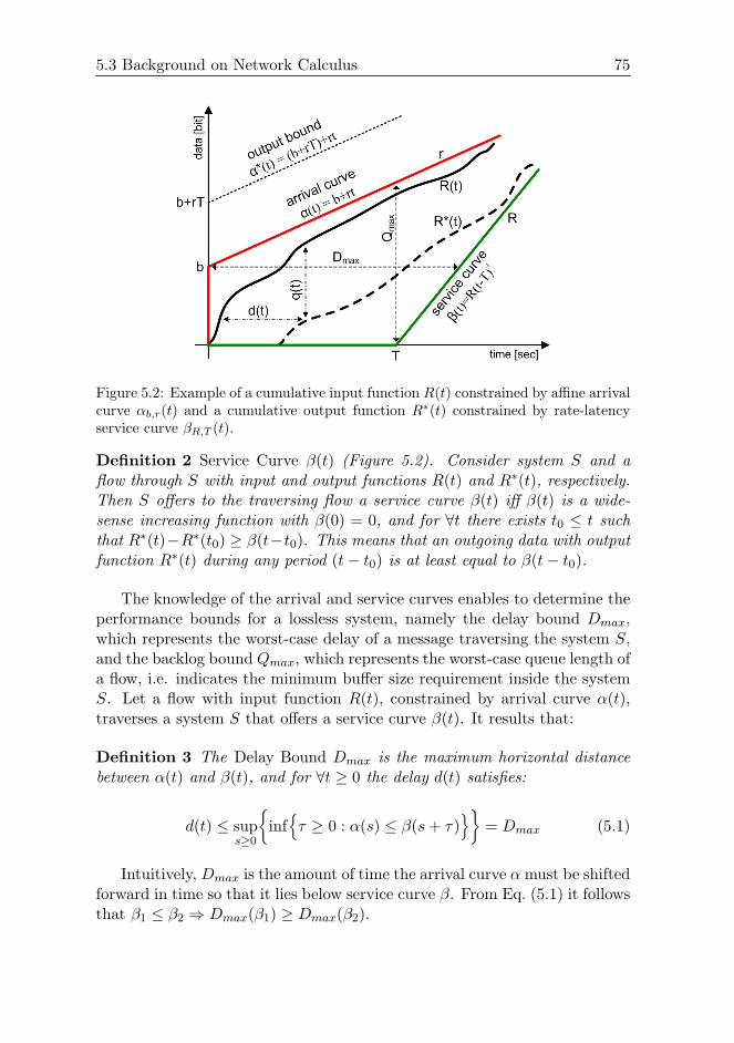
5.3 Background on Network Calculus 75
Figure 5.2: Example of a cumulative input function R(t) constrained by affine arrivalcurve αb,r(t) and a cumulative output function R∗(t) constrained by rate-latencyservice curve βR,T (t).
Definition 2 Service Curve β(t) (Figure 5.2). Consider system S and aflow through S with input and output functions R(t) and R∗(t), respectively.Then S offers to the traversing flow a service curve β(t) iff β(t) is a wide-sense increasing function with β(0) = 0, and for ∀t there exists t0 ≤ t suchthat R∗(t)−R∗(t0) ≥ β(t−t0). This means that an outgoing data with outputfunction R∗(t) during any period (t− t0) is at least equal to β(t− t0).
The knowledge of the arrival and service curves enables to determine theperformance bounds for a lossless system, namely the delay bound Dmax,which represents the worst-case delay of a message traversing the system S,and the backlog bound Qmax, which represents the worst-case queue length ofa flow, i.e. indicates the minimum buffer size requirement inside the systemS. Let a flow with input function R(t), constrained by arrival curve α(t),traverses a system S that offers a service curve β(t). It results that:
Definition 3 The Delay Bound Dmax is the maximum horizontal distancebetween α(t) and β(t), and for ∀t ≥ 0 the delay d(t) satisfies:
d(t) ≤ sups≥0
infτ ≥ 0 : α(s) ≤ β(s+ τ)
= Dmax (5.1)
Intuitively, Dmax is the amount of time the arrival curve α must be shiftedforward in time so that it lies below service curve β. From Eq. (5.1) it followsthat β1 ≤ β2 ⇒ Dmax(β1) ≥ Dmax(β2).
76 Chapter 5 Dimensioning and worst-case analysis of cluster-tree WSNs
Definition 4 The Backlog Bound Qmax is the maximum vertical distancebetween α(t) and β(t), and for ∀t ≥ 0 the backlog q(t) satisfies:
q(t) ≤ sups≥0
α(s)− β(s)
= Qmax (5.2)
In Network Calculus, it is also possible to express an upper bound for anoutgoing data with output function R∗(t), called output bound.
Definition 5 Output Bound α∗(t). Assume that a flow with input functionR(t), constrained by arrival curve α(t), traverses a system S that offers aservice curve β(t). Then, the output function R∗(t) is upper bounded by thefollowing output bound α∗(t):
α∗(t) ≤ (α β) ≥ α(t) (5.3)
where is the min-plus deconvolution defined for f, g ∈ F, where F is theset of wide sense increasing functions, as:
(f g)(t) = sups≥0
f(t+ s)− g(s)
for ∀t ∈ R (5.4)
So far a system S has been handled as a single buffered node (Figure 5.1).However, system S might also be a sequence of nodes or even a completenetwork. In this case, the concatenation theorem enables to investigate a setof nodes in sequence as a single node.
Definition 6 Concatenation Theorem. Assume a flow with input functionR(t) traversing system S1 and S2 in sequence, where S1 offers service curveβ1(t) and S2 offers β2(t). Then the concatenation of these two systems offersthe following single service curve β(t) to the traversing flow:
β(t) = (β1 ⊗ β2)(t) = (β2 ⊗ β1)(t) (5.5)
where ⊗ is the min-plus convolution defined for f, g ∈ F as:
(f ⊗ g)(t) = inf0≤s≤t
f(t− s) + g(s)
for ∀t ≥ 0 (5.6)
Min-plus convolution has several important properties, including beingcommutative and associative. Furthermore, convolution of concave curves is
5.3 Background on Network Calculus 77
equal to their minimum [59]. It can be also shown that service curve β andarrival curve α can be expressed using a min-plus convolution as follows:
R∗ ≥ (R⊗ β)(t) = inf0≤s≤t
R(t− s) + β(s)
for ∀t ≥ 0
R ≤ (R⊗ α)(t) = inf0≤s≤t
R(t− s) + α(s)
for ∀t ≥ 0
Due to the aggregation of the data flows in the direction of the sink, eachrouter must provide a service curve β(t) to the aggregated data flow. Thus,the delay and backlog bounds are computed for the aggregated data flowtraversing the router. On the other hand, using the aggregate schedulingtheorem, tighter bounds can be computed for each individual data flowtraversing the network. In this work, both approaches (i.e. aggregated flowper router and individual flow over network) are used to compare the results.
Definition 7 Aggregate Scheduling Theorem. Consider a lossless nodemultiplexing two data flows, 1 and 2, in FIFO order. Assume that flow 2is constrained by the arrival curve α2(t) and the node guarantees a servicecurve β(t) to the aggregate of these two flows. Define the family of functionsas:
βeq1 (t,Θ) =
[β(t)− α2(t−Θ)
]+· 1t>Θ (5.7)
where notation 1expr is equal to 1 if expr is true, and 0 otherwise, and (x)+
denotes max(0, x). Then for ∀Θ ≥ 0, βeq1 (t,Θ) is an equivalent service curve
guaranteed for flow 1.
So far an abstract Network Calculus model has been considered. Theaccuracy of the worst-case bounds depends on how tightly the selected arrivaland service curves follow the real network behaviour. Different types ofarrival and service curves have been proposed in Network Calculus (e.g. [31,57]). However, the affine arrival curve and rate-latency service curve arethe most used (as illustrated in Figure 5.2), since they lead to a fair trade-off between computing complexity and accuracy (approximation to the realsystem behaviour), as it will be shown in this chapter.
The affine arrival curve (Figure 5.2) is defined as αb,r(t) = b + r · tfor ∀t > 0 and 0 otherwise, where b is called burst tolerance, which is themaximum number of bits that can arrive simultaneously at a given time tothe system S, and r is the average data rate. This type of arrival curverepresents a data traffic based on the average sensing rate with short-term
78 Chapter 5 Dimensioning and worst-case analysis of cluster-tree WSNs
fluctuations given by the burst tolerance, i.e. it allows a node to send b bitsat once, but no more than an average of r bits per second over a long run.
The rate-latency service curve is defined as βR,T (t) = R · (t− T )+, whereR ≥ r is the guaranteed forwarding rate, T is the maximum latency offorwarding data (both depend on the nodes features, such as processing speedand resource allocation mechanism). If r > R, the bounds are infinite.
Hereafter, a system S is considered as the one that guarantees a rate-latency service curve βR,T (t) and that stores incoming data in a FIFO buffer.Then, the performance bounds Dmax and Qmax (see Figure 5.2 for additionalintuition) guaranteed to the data flow, constrained by the affine arrival curveαb,r(t) and traversing system S, are easily computed as:
Dmax =b
R+ T Qmax = b+ r · T (5.8)
Note that the first term b/R is interpreted as the part of the delay due tothe burstiness of the incoming data, whereas T is due to the latency of thenode.
An application of Eq. (5.3) to a data flow constrained by affine arrivalcurve αb,r(t) and traversing system S guaranteeing a rate-latency servicecurve βR,T (t), the output bound of this data flow is expressed as (the proofcan be found in [66]):
α∗(t) = αb,r(t)βR,T (t) = αb,r(t)+ r ·T = (b+ r ·T )+ r · t = b∗+ r∗ · t (5.9)
According to the aggregate scheduling theorem, α2(t) is a affine arrivalcurve and β(t) is a rate-latency service curve, then an equivalent service curvefor data flow 1 is expressed as:
βeq1 (t,Θ) = (R− r2) ·
[t−
(b2 + r2(T −Θ)R− r2
+ T)]+
· 1t>Θ (5.10)
Hereafter, we omit repeating that arrive curves are affine and servicecurves are rate-latency, and that all curves are functions of time wheneverdoing so does not generate ambiguity.

5.4 System model 79
5.4 System model
This section defines general cluster-tree topology and data flow models thatwill be considered in the following analysis. It also elaborates on the worst-case cluster scheduling; that is, the time sequence of clusters’ active portionsleading to the worst-case end-to-end delay for a message to be routed to thesink. To ensure predictable performance of a WSN, the network topology anddata flows must be bounded. To provide closed-form recurrent expressionsfor computing the worst-case performance bounds in a WSN, the networktopology and data load must be balanced.
5.4.1 Cluster-tree topology model
Like in Chapter 4, for achieving predictable resource guarantees, the cluster-tree is considered as a logical topology of WSNs. The cluster-tree topologymodel has been defined in Section 4.3.1. In this chapter, the routers and end-nodes are referred to as Rij (i.e the jth router at depth i) and N , respectively.The routers and end-nodes having sensing capabilities are generally referredto as sensor nodes. The depth of a node is defined as the number of logicalhops from that node to the root. Note that the root is at depth zero and, byconvention, trees grow down.
This section aims at specifying the worst-case cluster-tree topology whichcontains the maximum number of nodes in the network, i.e. the networktopology configuration that leads to the worst-case performance. In theworst-case, when the maximum depth is reached, and all routers have themaximum number of associated child end-nodes and routers, the topologywill be balanced (regular). However, a particular WSN can have unbalancedor even dynamically changing cluster-tree topology, but it can never exceedthe worst-case topology, in terms of maximum depth and number of childrouters/end-nodes. The irregularities in a particular topology introduce somepessimism to the analysis. On the other hand, for any network deploymentcan be found several cluster-tree topologies. Depending on the application,the system designer should select the most regular topology in design timeto reduce the pessimism of the worst-case results.
The worst-case cluster-tree topology is defined by the following threeparameters (derived from the ZigBee [10] specification):
NMAXend−node Maximum number of end-nodes that can be associated to
a router and have been allocated resource guarantees (e.g.time slots or bandwidth).
80 Chapter 5 Dimensioning and worst-case analysis of cluster-tree WSNs
NMAXrouter Maximum number of child routers that can be associated to
a parent router and have been allocated resource guarantees.
H Height of the tree, i.e. the maximum number of logical hopsfor a message from the deepest router to reach the root(including the root as a final hop). A network with onlya root has a height of zero, and the maximum depth of anend-node is H + 1.
Note that a cluster-tree WSN may contain additional nodes per routerthan those defined by NMAX
router and NMAXend−node parameters. However, these
additional nodes cannot be granted guaranteed resources.Data gathering (all-to-one) and data dissemination (one-to-all) are two
fundamental traffic patterns in WSNs [67]. This chapter only assumes theformer, so called convergecast, where the sink gathers sensory data fromall sensor nodes. The sink is considered as an autonomous and topology-independent static or mobile entity. The mobile behaviour means that asink moves arbitrarily within a cluster-tree WSN and can be associated toany router within communication range. The router to which the sink isassociated in a given moment is referred to as sink router. There can bemore than one mobile sink in a WSN, but only one is active (i.e. gathers thesensory data) at a given time. Hence, another parameter, Hsink ∈ (0, H),is specified to represent the maximum depth of the sink router in a cluster-tree topology, at a given moment. Note that the sink can be also staticallyattached to the root, i.e. Hsink = 0. In this case, the network contains onlydata links in upstream direction (i.e. from child nodes to the parent router)as was presented in [68].
The terminology and conventions are illustrated in Figure 5.3, corre-sponding to the worst-case configuration where H = 2, NMAX
end−node = 3,NMAX
router = 2, and Hsink = 2. The open arrows depict the data links inupstream or downstream direction.
5.4.2 Data flow model
This chapter assumes that all data traffic is routed to the sink router withoutany in-network processing on the way. In the worst-case, all sensor nodes areassumed to contribute equally to the network load, sensing and transmittingsensory data upper bounded by the affine arrival curve αdata = bdata +rdata · t(Figure 5.4), where bdata is the burst tolerance and rdata is the average datarate. The affine arrival curve can represent any type of traffic, assuming thatit can be bounded. It can represent a periodic or aperiodic traffic [69], or
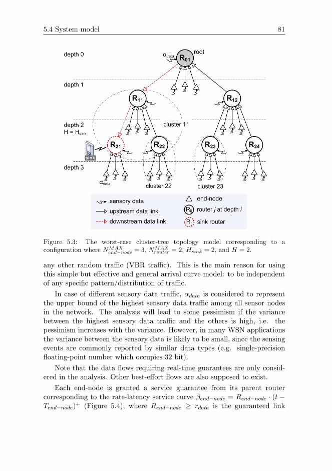
5.4 System model 81
Figure 5.3: The worst-case cluster-tree topology model corresponding to aconfiguration where NMAX
end−node = 3, NMAXrouter = 2, Hsink = 2, and H = 2.
any other random traffic (VBR traffic). This is the main reason for usingthis simple but effective and general arrival curve model: to be independentof any specific pattern/distribution of traffic.
In case of different sensory data traffic, αdata is considered to representthe upper bound of the highest sensory data traffic among all sensor nodesin the network. The analysis will lead to some pessimism if the variancebetween the highest sensory data traffic and the others is high, i.e. thepessimism increases with the variance. However, in many WSN applicationsthe variance between the sensory data is likely to be small, since the sensingevents are commonly reported by similar data types (e.g. single-precisionfloating-point number which occupies 32 bit).
Note that the data flows requiring real-time guarantees are only consid-ered in the analysis. Other best-effort flows are also supposed to exist.
Each end-node is granted a service guarantee from its parent routercorresponding to the rate-latency service curve βend−node = Rend−node · (t −Tend−node)+ (Figure 5.4), where Rend−node ≥ rdata is the guaranteed link
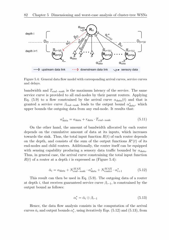
82 Chapter 5 Dimensioning and worst-case analysis of cluster-tree WSNs
Figure 5.4: General data flow model with corresponding arrival curves, service curvesand delays.
bandwidth and Tend−node is the maximum latency of the service. The sameservice curve is provided to all end-nodes by their parent routers. ApplyingEq. (5.9) to a flow constrained by the arrival curve αdata(t) and that isgranted a service curve βend−node leads to the output bound α∗data, whichupper bounds the outgoing data from any end-node. It results that:
α∗data = αdata + rdata · Tend−node (5.11)
On the other hand, the amount of bandwidth allocated by each routerdepends on the cumulative amount of data at its inputs, which increasestowards the sink. Thus, the total input function R(t) of each router dependson the depth, and consists of the sum of the output functions R∗(t) of itsend-nodes and child routers. Additionally, the router itself can be equippedwith sensing capability producing a sensory data traffic bounded by αdata.Thus, in general case, the arrival curve constraining the total input functionR(t) of a router at a depth i is expressed as (Figure 5.4):
αi = αdata +NMAXend−node · α∗data +NMAX
router · α∗i+1 (5.12)
This result can then be used in Eq. (5.9). The outgoing data of a routerat depth i, that receives guaranteed service curve βi−1, is constrained by theoutput bound as follows:
α∗i = αi βi−1 (5.13)
Hence, the data flow analysis consists in the computation of the arrivalcurves αi and output bounds α∗i , using iteratively Eqs. (5.12) and (5.13), from
5.4 System model 83
the deepest routers until reaching the sink router. After that, the resourcerequirements of each router, in terms of buffer requirement Qi and bandwidthrequirement Ri, and the worst-case end-to-end delay bounds are computed.
In cluster-tree WSNs, where the sink can be associated to any router, datamay flow in the upstream and downstream directions. In the upstream case,data is sent from the child nodes to its parent router (so called upstreamdirection), and the parent router must reserve enough bandwidth for theoutgoing data of its child nodes. On the contrary, in the downstream case,data is sent from a parent router to its child router (so called downstreamdirection), and the parent router must reserve enough bandwidth for itsown outgoing data. Note that if the sink is associated to the root, i.e.Hsink = 0, all data flows only in upstream direction. In what follows, theupstream and downstream directions are marked by the subscripts U and D,respectively (e.g. α∗iU , αiD). Each router at depth i provides two types ofservice curves (i.e. βiU for data in the upstream direction and βiD for datain the downstream direction) to its child routers at depth i + 1, which areexpressed as:
βiU = RiU · (t− TiU )+ βiD = RiD · (t− TiD)+ (5.14)
where Ri is the guaranteed link bandwidth, and Ti is the maximum latencythat a data must wait for a service. To ensure the balanced propertiesof the worst-case cluster-tree topology assumed in this methodology, thesame upstream/downstream service curves must be guaranteed to all up-stream/downstream data at a given depth. The balanced properties meansthat the worst-case cluster-topology and worst-case data flows are balancedsuch that the upstream/downstream routers in a given depth allocate and usethe same resources. Note that the routers forwarding data in the upstreamdirection are referred to as upstream routers (e.g. R12 orR23 in the example inFigure 5.3) whereas the routers forwarding data in the downstream directionare referred to as downstream routers (e.g. R01 or R11). In the same way,the data links between nodes are referred to as upstream or downstream.
5.4.3 Time Division Cluster Schedule
To avoid collisions between clusters, it is mandatory to schedule the clusters’active portions in an ordered sequence that is called Time Division ClusterSchedule (TDCS) (Section 4.4). In case of single collision domain, the TDCSmust be non-overlapping, i.e. only one cluster can be active at any time.Hence, the period of TDCS is given by the number of clusters and the length
84 Chapter 5 Dimensioning and worst-case analysis of cluster-tree WSNs
of their active portions. On the contrary, in a network with multiple collisiondomains, the clusters from different non-overlapping collision domains maybe active at the same time. It is easy to see that the period of overlappingTDCS is shorter (some active portions can run simultaneously) than theperiod of non-overlapping TDCS. Hence, the non-overlapping TDCS providesthe worst-case performance bounds, which are the objective of this chapter.Note that the non-overlapping TDCS can be more pessimistic in networkswith multiple collision domains.
The TDCS significantly affects the resource requirements and delaybounds in cluster-tree WSNs. The number of feasible non-overlapping TDCSsin a network with n routers is equal to the number of permutations given byn factorial (n!). Note that for each data flow originated in a given node, thereis a corresponding best-case/worst-case TDCS that minimizes/maximizes theend-to-end delay of that flow, respectively. Thus, it is impossible to determinea general best-case or worst-case TDCS meeting the requirements of all dataflows. On one hand, the best-case TDCS of a data flow originated in a nodex comprises the consecutive sequence of active portions corresponding to theordered sequence of the clusters traversed along the routing path from x tothe sink. On the other hand, the worst-case TDCS (WC-TDCS) comprisesthe same ordered sequence of active portions, but in the reverse order, whichmeans starting from the sink backward to the node x. The active portionsof other clusters, which are not on the routing path, are appended before orafter the previously formed sequence in arbitrary order such that a completeWC-TDCS for a given flow is produced. Using the proposed methodologybased on the balanced properties of cluster-tree topology model (i.e. balancedtopology with balanced load), the WSN resources are dimensioned for non-overlapping WC-TDCS of a data flow originated in the end-node that isfarthest from the sink (i.e. a flow along the longest routing path in a WSN).Within a period of WC-TDCS the messages belonging to this data flow goonly one hop forward. Note that for a particular cluster-tree WSN, theoverlapping or non-overlapping application-specific TDCS, which achievesbetter performance bounds than WC-TDCS, can be found. However, theinterest is in the worst-case performance bounds of general WSNs such thatnon-overlapping WC-TDCS is the objective.
Let us consider the example in Figure 5.3, where an end-node of routerR24 sends sensory data to the sink (that is associated to router R21), i.e. adata flow along the longest routing path in the WSN. The non-overlappingbest-case TDCS for this flow comprises the continuous sequence of activeportions of clusters 24, 12, 01 and 11. On the contrary, the WC-TDCScomprises the same sequence but in the reverse order, i.e. active portions of
5.5 Data flow analysis 85
clusters 11, 01, 12 and 24. The active portions of other clusters (i.e. clusters21, 22 and 23) are appended in arbitrary order such that the complete WC-TDCS is the sequence of active portions of clusters 22, 11, 01, 12, 24, 21and 23, for example.
To reduce the resource requirements of the routers, the priority rule hasbeen introduced in Section 4.4.1. Using this rule, the end-to-end delay of adata flow can be reduced by one period of TDCS at a router which handlesthe links in both directions for a given data flow.
5.5 Data flow analysis
This section serves as a basic building block for Section 5.6. Recurrentequations of the incoming or outgoing data in upstream or downstreamdirection as a function of the router’s depth are derived, considering thegeneral cluster-tree topology model presented in Section 5.4. It is assumedthat the end-nodes have sensing capabilities, but the sensing capabilities ofthe routers are optional. Therefore, a binary variable ω is introduced. Thevalue of ω is equal to 1 if routers have sensing capabilities; otherwise ω isequal to 0.
5.5.1 Upstream direction
First, the arrival curves of the incoming data in upstream direction αiU
and the upper bounds of the outgoing data in upstream direction α∗iU areevaluated depth by depth, using the Network Calculus methodology, startingfrom depth H (i.e. the deepest routers). These derivations are based on thework [68]. The analysis considers the general queuing model for the upstreamdirection as illustrated in Figure 5.5.
Analysis of depth H+1
At depth H + 1, there is no router, there are only end-nodes generatedsensory data constrained by the arrival curve αdata. A parent router at depthH guarantees the service curve βend−node to each of its end-nodes. Thus,according to Eq. (5.11) the outgoing data of each end-node is constrained bythe output bound α∗data.
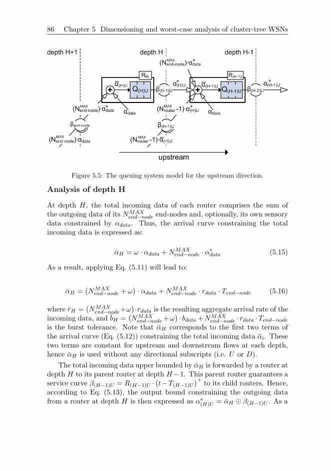
86 Chapter 5 Dimensioning and worst-case analysis of cluster-tree WSNs
Figure 5.5: The queuing system model for the upstream direction.
Analysis of depth H
At depth H, the total incoming data of each router comprises the sum ofthe outgoing data of its NMAX
end−node end-nodes and, optionally, its own sensorydata constrained by αdata. Thus, the arrival curve constraining the totalincoming data is expressed as:
αH = ω · αdata +NMAXend−node · α∗data (5.15)
As a result, applying Eq. (5.11) will lead to:
αH =(NMAX
end−node + ω)· αdata +NMAX
end−node · rdata · Tend−node (5.16)
where rH =(NMAX
end−node+ω)·rdata is the resulting aggregate arrival rate of the
incoming data, and bH =(NMAX
end−node +ω)· bdata +NMAX
end−node · rdata ·Tend−node
is the burst tolerance. Note that αH corresponds to the first two terms ofthe arrival curve (Eq. (5.12)) constraining the total incoming data αi. Thesetwo terms are constant for upstream and downstream flows at each depth,hence αH is used without any directional subscripts (i.e. U or D).
The total incoming data upper bounded by αH is forwarded by a router atdepth H to its parent router at depth H−1. This parent router guarantees aservice curve β(H−1)U = R(H−1)U ·
(t−T(H−1)U
)+ to its child routers. Hence,according to Eq. (5.13), the output bound constraining the outgoing datafrom a router at depth H is then expressed as α∗(H)U = αH β(H−1)U . As a
5.5 Data flow analysis 87
result, applying Eq. (5.9) will lead to:
α∗(H)U = αH + σ(H−1) (5.17)
where σ(H−1) = rH · T(H−1)U .
Analysis of depth H–1
The total incoming data of a router at depth H − 1 comprises the outgoingdata of its child router in addition to the data of its child end-nodes, and itsown (optional) sensory data. Thus, the arrival curve constraining the totalincoming data is expressed as α(H−1)U =
(ω · αdata + NMAX
end−node · α∗data
)+
NMAXrouter · α∗(H)U . As a result, using Eqs. (5.15) and (5.17) will lead to:
α(H−1)U =(NMAX
router + 1)· αH +NMAX
router · σ(H−1) (5.18)
The total incoming data upper bounded by α(H−1)U is forwarded by arouter at depth H−1 to its parent routers at depth H−2. This parent routerguarantees a service curve β(H−2)U to its child routers. Hence, according toEq. (5.13), the output bound constraining the outgoing data from a routerat depth H − 1 is then expressed as α∗(H−1)U = α(H−1)U β(H−2)U . As aresult, applying Eqs. (5.3) and (5.18) will lead to:
α∗(H−1)U =(NMAX
router + 1)· αH +NMAX
router · σ(H−1) + σ(H−2) (5.19)
where σ(H−2) =(NMAX
router + 1)· rH · T(H−2)U .
Analysis of depth H–2
Similarly to the previous case, the arrival curve constraining the totalincoming data of a router at depth H − 2 is expressed as:
α(H−2)U =
((NMAX
router)2 +NMAXrouter + 1
)· αH+
(NMAXrouter)2 · σ(H−1) +NMAX
router · σ(H−2)
(5.20)
The outgoing data forwarded from a router at depth H − 2 to its parentrouter at depth H − 3, providing a service curve β(H−3)U , is constraining by
88 Chapter 5 Dimensioning and worst-case analysis of cluster-tree WSNs
the output bound:
α∗(H−2)U = α(H−2)U + σ(H−3) (5.21)
where σ(H−3) =((NMAX
router)2 +NMAXrouter + 1
)· rH · T(H−3)U .
Analysis of general depth i
By recurrence, it can be easily proved that the arrival curve, constraining thetotal incoming data in upstream direction of each router at a given depth i,is expressed as follows:
αiU =H−i∑j=0
(NMAXrouter)j · αH +
H−i∑j=1
((NMAX
router)j · σi+j−1)
(5.22)
for ∀i, 0 ≤ i ≤ H, where σn =∑H−(n+1)
k=0 (NMAXrouter)k · rH · TnU .
The output bound constraining the outgoing data in upstream directionfrom each child router at depth i, receiving a service curve β(i−1) from aparent router at depth i− 1, is expressed as:
α∗iU = αiU + σi−1 =H−i∑j=0
(NMAXrouter)j · αH +
H−i∑j=0
((NMAX
router)j · σi+j−1)
(5.23)
for ∀i, 0 < i ≤ H.
5.5.2 Downstream direction
In this section, the arrival curves of the incoming data in downstreamdirection αiD and the upper bounds of the outgoing data in downstreamdirection α∗iD is evaluated depth by depth, using the Network Calculusmethodology, starting from depth 0 (i.e. the root). The analysis considers thegeneral queuing model for downstream direction as illustrated in Figure 5.6.
Analysis of depth 0
At depth 0, there is only one router, the root, and its total incoming datacomprises the sum of the outgoing data of its end-nodes, the sum of theoutgoing data in upstream direction of its (NMAX
router − 1) child routers, and,optionally, its own sensory data constrained by αdata. Thus, the arrival curve
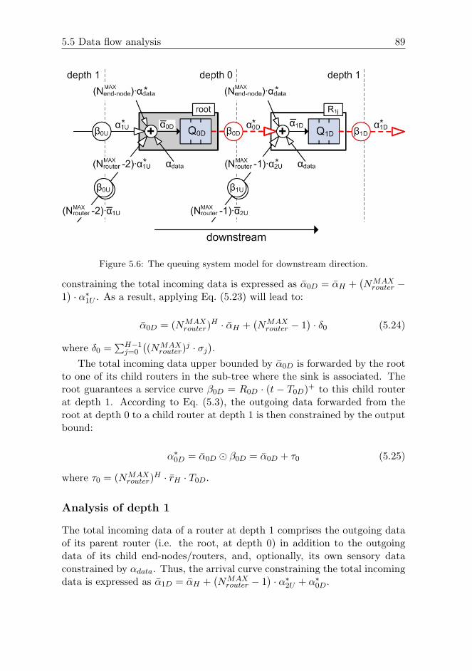
5.5 Data flow analysis 89
Figure 5.6: The queuing system model for downstream direction.
constraining the total incoming data is expressed as α0D = αH +(NMAX
router −1)· α∗1U . As a result, applying Eq. (5.23) will lead to:
α0D = (NMAXrouter)H · αH +
(NMAX
router − 1)· δ0 (5.24)
where δ0 =∑H−1
j=0
((NMAX
router)j · σj).
The total incoming data upper bounded by α0D is forwarded by the rootto one of its child routers in the sub-tree where the sink is associated. Theroot guarantees a service curve β0D = R0D · (t − T0D)+ to this child routerat depth 1. According to Eq. (5.3), the outgoing data forwarded from theroot at depth 0 to a child router at depth 1 is then constrained by the outputbound:
α∗0D = α0D β0D = α0D + τ0 (5.25)
where τ0 = (NMAXrouter)H · rH · T0D.
Analysis of depth 1
The total incoming data of a router at depth 1 comprises the outgoing dataof its parent router (i.e. the root, at depth 0) in addition to the outgoingdata of its child end-nodes/routers, and, optionally, its own sensory dataconstrained by αdata. Thus, the arrival curve constraining the total incomingdata is expressed as α1D = αH +
(NMAX
router − 1)· α∗2U + α∗0D.

90 Chapter 5 Dimensioning and worst-case analysis of cluster-tree WSNs
As a result, applying Eqs. (5.23) and (5.25) will lead to:
α1D =
((NMAX
router)H + (NMAXrouter)H−1
)· αH+(
NMAXrouter − 1
)·(δ0 + δ1
)+ τ0
(5.26)
where δ1 =∑H−2
j=0
((NMAX
router)j · σj+1).
The total incoming data upper bounded by α1D is forwarded by therouter at depth 1 to one of its child routers in the sub-tree where thesink is associated. The parent router guarantees a service curve β1D =R1D · (t − T1D)+ to this child router at depth 2. According to Eq. (5.3),the outgoing data forwarded from the router at depth 1 to a child router atdepth 2 is constrained by the output bound:
α∗1D = α1D β1D = α1D + τ1 (5.27)
where τ1 =((NMAX
router)H + (NMAXrouter)H−1
)· rH · T1D.
Analysis of depth 2
Similar to the previous case, the arrival curve constraining the total incomingdata of the router at depth 2 is expressed as α2D = αH +
(NMAX
router−1)·α∗3U +
α∗1D. As a result, applying Eqs. (5.23) and (5.27) will lead to:
α2D =
((NMAX
router)H + (NMAXrouter)H−1 + (NMAX
router)H−2)· αH+(
NMAXrouter−
)·(δ0 + δ1 + δ2
)+ τ0 + τ1
(5.28)
where δ2 =∑H−3
j=0
((NMAX
router)j · σj+2).
The outgoing data from the router at depth 2, guaranteeing a servicecurve β2D = R2D · (t− T2D)+, to a child router at depth 3 is upper boundedby the output bound:
α∗2D = α2D β2D = α2D + τ2 (5.29)
where τ2 =((NMAX
router)H + (NMAXrouter)H−1 + (NMAX
router)H−2)· rH · T2D.
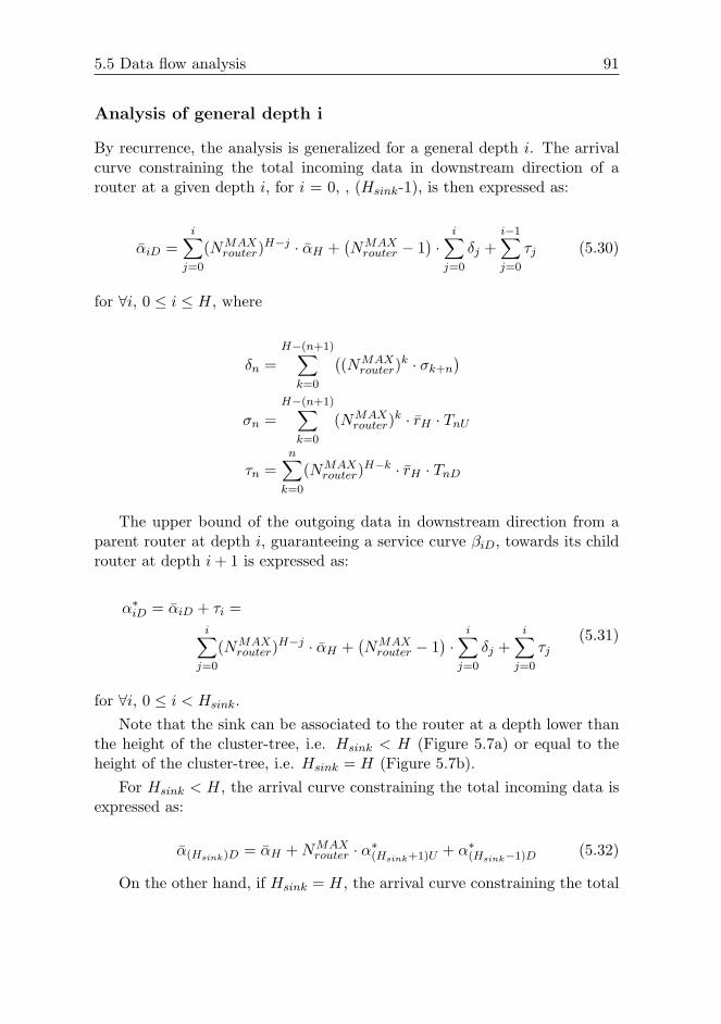
5.5 Data flow analysis 91
Analysis of general depth i
By recurrence, the analysis is generalized for a general depth i. The arrivalcurve constraining the total incoming data in downstream direction of arouter at a given depth i, for i = 0, , (Hsink-1), is then expressed as:
αiD =i∑
j=0
(NMAXrouter)H−j · αH +
(NMAX
router − 1)·
i∑j=0
δj +i−1∑j=0
τj (5.30)
for ∀i, 0 ≤ i ≤ H, where
δn =H−(n+1)∑
k=0
((NMAX
router)k · σk+n
)
σn =H−(n+1)∑
k=0
(NMAXrouter)k · rH · TnU
τn =n∑
k=0
(NMAXrouter)H−k · rH · TnD
The upper bound of the outgoing data in downstream direction from aparent router at depth i, guaranteeing a service curve βiD, towards its childrouter at depth i+ 1 is expressed as:
α∗iD = αiD + τi =i∑
j=0
(NMAXrouter)H−j · αH +
(NMAX
router − 1)·
i∑j=0
δj +i∑
j=0
τj(5.31)
for ∀i, 0 ≤ i < Hsink.Note that the sink can be associated to the router at a depth lower than
the height of the cluster-tree, i.e. Hsink < H (Figure 5.7a) or equal to theheight of the cluster-tree, i.e. Hsink = H (Figure 5.7b).
For Hsink < H, the arrival curve constraining the total incoming data isexpressed as:
α(Hsink)D = αH +NMAXrouter · α∗(Hsink+1)U + α∗(Hsink−1)D (5.32)
On the other hand, if Hsink = H, the arrival curve constraining the total
92 Chapter 5 Dimensioning and worst-case analysis of cluster-tree WSNs
(a) Hsink = 1 < H (depth=1) (b) Hsink = 2 = H (depth=2)
Figure 5.7: The locations of a sink router and correspondent data flows.
incoming data is expressed as:
α(Hsink)D = αH + α∗(Hsink−1)D (5.33)
5.6 Worst-case network dimensioning
Supporting time-sensitive WSN applications implies to predict and guaranteebounded (worst-case) end-to-end communication delays. To ensure boundedend-to-end delays and to avoid buffer overflow, network resources must beknown in advance, and dimensioned along the path from a source to a sink.In this section, the upper bounds on bandwidth and buffer requirements, andper-hop and end-to-end delays for both upstream and downstream directionsare derived.
5.6.1 Per-router resources analysis
The aim is at specifying the minimum bandwidth of each upstream anddownstream data links and the minimum buffer size at each router neededto store the bulk of data incoming through the router’s inputs.
Bandwidth requirements
Consider a parent router at depth i providing a service curve βiU or βiD to itschild routers at depth i+1 in upstream or downstream direction, respectively(see Figure 5.3).
5.6 Worst-case network dimensioning 93
In the upstream case, the outgoing data of a child router at depth i +1 is constrained by the output bound α∗(i+1)U and dispatched through theupstream link to its parent router at depth i. Thus, to ensure a boundeddelay, the guaranteed amount of bandwidth RiU must be greater than orequal to the outgoing data rate r∗(i+1)U . As a result, applying Eqs. (5.16)and (5.23) will lead to:
RiU ≥ r∗(i+1)U = r(i+1)U =H−(i+1)∑
j=0
(NMAXrouter)j · rH =
ΩiU (H,NMAXrouter) ·
(NMAX
end−node + ω)· rdata
(5.34)
for ∀i, 0 ≤ i < H.The ΩiU (H,NMAX
router) is called the upstream bandwidth increase factor ata given depth i. This factor increases with the depth and NMAX
router, and itrepresents the ratio of the additional bandwidth that a router, at a depthi, must guarantee to each of its child routers in the upstream direction ascompared to the bandwidth required by a router at depth H.
In the downstream case, the total incoming data of the parent routerat depth i is constrained by the arrival curve αiD and dispatched througha downstream link to its child router. Thus, to ensure a bounded delay,the guaranteed amount of bandwidth RiD must be greater than or equal tothe arrival rate of total input flow riD. As a result, applying Eqs. (5.16)and (5.30) will lead to:
RiD ≥ riD = r∗iD =i∑
j=0
(NMAXrouter)H−j · rH =
ΩiD(H,NMAXrouter) ·
(NMAX
end−node + ω)· rdata
(5.35)
for ∀i, 0 ≤ i < Hsink.Similarly to the previous case, the ΩiD(H,NMAX
router) is called the down-stream bandwidth increase factor at a given depth i. This factor representsthe ratio of the additional bandwidth that a router, at depth i, mustguarantee to its child router in downstream direction as compared to thebandwidth required by a router at the depth H. Note that it is possible todetermine the total number of routers in a cluster-tree WSN using the down-
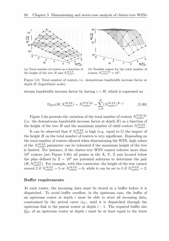
94 Chapter 5 Dimensioning and worst-case analysis of cluster-tree WSNs
(a) Total number of routers as a function ofthe height of the tree H and NMAX
router.(b) Feasible region for the total number ofrouters NTOTAL
router = 102.
Figure 5.8: Total number of routers, i.e. downstream bandwidth increase factor atdepth H (logarithmic scale).
stream bandwidth increase factor by having i = H, which is expressed as:
ΩHD(H,NMAXrouter) = NTOTAL
router =H∑
j=0
(NMAXrouter)H−j (5.36)
Figure 5.8a presents the variation of the total number of routers NTOTALrouter
(i.e. the downstream bandwidth increase factor at depth H) as a function ofthe height of the tree H and the maximum number of child routers NMAX
router.It can be observed that if NMAX
router is high (e.g. equal to 5) the impact ofthe height H on the total number of routers is very significant. Depending onthe total number of routers allowed when dimensioning the WSN, high valuesof the NMAX
router parameter can be tolerated if the maximum height of the treeis limited. For instance, if the cluster-tree WSN cannot tolerate more than102 routers (see Figure 5.8b) all points in the X, Y, Z axis located belowthe plan defined by Z = 102 are potential solutions to determine the pair(H,NMAX
router). For example, with this constraint, the height of the tree cannotexceed 2 if NMAX
router = 5 or NMAXrouter = 6, while it can be set to 5 if NMAX
router = 2.
Buffer requirements
At each router, the incoming data must be stored in a buffer before it isdispatched. To avoid buffer overflow, in the upstream case, the buffer ofan upstream router at depth i must be able to store all incoming data,constrained by the arrival curve αiU , until it is dispatched through theupstream link to the parent router at depth i − 1. The required buffer sizeQiU of an upstream router at depth i must be at least equal to the burst
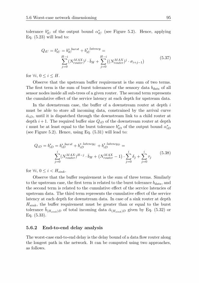
5.6 Worst-case network dimensioning 95
tolerance b∗iU of the output bound α∗iU (see Figure 5.2). Hence, applyingEq. (5.23) will lead to:
QiU = b∗iU = b∗ burstiU + b∗ latency
iU =H−i∑j=0
(NMAXrouter)j · bH +
H−i∑j=0
((NMAX
router)j · σi+j−1) (5.37)
for ∀i, 0 ≤ i ≤ H.Observe that the upstream buffer requirement is the sum of two terms.
The first term is the sum of burst tolerances of the sensory data bdata of allsensor nodes inside all sub-trees of a given router. The second term representsthe cumulative effect of the service latency at each depth for upstream data.
In the downstream case, the buffer of a downstream router at depth imust be able to store all incoming data, constrained by the arrival curveαiD, until it is dispatched through the downstream link to a child router atdepth i+ 1. The required buffer size QiD of the downstream router at depthi must be at least equal to the burst tolerance b∗iD of the output bound α∗iD(see Figure 5.2). Hence, using Eq. (5.31) will lead to:
QiD = b∗iD = b∗ burstiD + b∗ latencyU
iD + b∗ latencyDiD =
i∑j=0
(NMAXrouter)H−j · bH +
(NMAX
router − 1)·
i∑j=0
δj +i∑
j=0
τj(5.38)
for ∀i, 0 ≤ i < Hsink.Observe that the buffer requirement is the sum of three terms. Similarly
to the upstream case, the first term is related to the burst tolerance bdata, andthe second term is related to the cumulative effect of the service latencies ofupstream data. The third term represents the cumulative effect of the servicelatency at each depth for downstream data. In case of a sink router at depthHsink, the buffer requirement must be greater than or equal to the bursttolerance b(Hsink)D of total incoming data α(Hsink)D given by Eq. (5.32) orEq. (5.33).
5.6.2 End-to-end delay analysis
The worst-case end-to-end delay is the delay bound of a data flow router alongthe longest path in the network. It can be computed using two approaches,as follows.
96 Chapter 5 Dimensioning and worst-case analysis of cluster-tree WSNs
Per-hop end-to-end delay
The first approach consists in computing the per-hop delay bounds of theaggregate flows, and then deducing the end-to-end delay bound as the sumof per-hop delays. In the upstream case, according to Eq. (5.8) the delaybound between a child router at depth i and its parent router at depthi− 1 guaranteeing service curve β(i−1)U is expressed as DiU = biU/R(i−1)U +T(i−1)U . On the other hand, in the downstream case, the delay bound betweena parent router at depth i, which guarantees service curve βiD to its totalincoming data constrained by arrival curve αiD, and its child router at depthi+ 1 is expressed as DiD = biD/RiD +TiD. Hence, the worst-case end-to-enddelay is the sum of all per-hop delay bounds along the longest routing path,as follows:
De2e = Dend−node +H∑
i=1
DiU +Hsink−1∑
i=0
DiD (5.39)
where Dend−node = bdata/Rend−node + Tend−node is the delay bound betweenan end-node and its parent router.
This approach is a bit pessimistic, since the delay bound at each routeris computed for the aggregation of all incoming flows. Tighter end-to-enddelay bounds can be computed for individual flows, as described next.
Per-flow end-to-end delay
The idea of this approach is to derive the service curves guaranteed to aparticular individual flow f by the routers along the path, using the aggregatescheduling theorem in Eq. (5.10), and then deduce the network-wide servicecurve for flow f based on the concatenation theorem. Finally, according toEq. (5.8), the end-to-end delay bound of a given flow f is computed usingthe network-wide service curve applied to the arrival curve of the incomingflow. The worst-case end-to-end delay is equal to the delay bound of a dataflow along the longest routing path in the network. This technique has beenused in [59].
Consider a consecutive sequence of routers along the longest routing path(e.g. from an end-node of router R24 to the sink router R21 in Figure 5.3).The per-flow approach to the worst-case end-to-end delay is based on thefollowing algorithm.
5.6 Worst-case network dimensioning 97
1. Start from the sink router. If Hsink = 0 then the index variable last = 0and the network-wide service curve βw = βlastU ; else (i.e. 1 ≤ Hsink <H) last = Hsink − 1, βw = βlastD, and go to step 4.
2. The service curve βw is guaranteed to the aggregate of incomingupstream flows of an upstream router at depth last+1 (i.e. NMAX
router flowsfrom child routers at depth last + 2, NMAX
end−node flows from end-nodes,and optional own sensory data). Using the aggregate scheduling inEq. (5.10), the equivalent service curve βeq is computed for the outgoingflow of a router at depth last+ 2 upper bounded by α∗(last+2)U .
3. Using the concatenation theorem in Eq. (5.5), replace βw = βeq ⊗β(last+1)U since the concatenation is also service curve for the outgoingflow of a router at depth last + 2. The length of the router’s tandemis then reduced by one. Increase the variable last = last+ 1. If last =H − 1, then go to step 7; else go to step 2.
4. The service curve βw is guaranteed to the aggregate of incomingupstream/downstream flows of the downstream router at depth last.Using the aggregate scheduling in Eq. (5.10), the equivalent servicecurve βeq is computed for the incoming downstream flow of thedownstream router upper bounded by α∗(last−1)D.
5. Using the concatenation theorem in Eq. (5.5), replace βw = βeq ⊗β(last−1)D since the concatenation is also service curve guaranteed to theoutgoing downstream flow of the downstream router at depth last− 1.The length of the router’s tandem is then reduced by one. Decreasethe variable last = last − 1. If last = 0, then go to step 6; else go tostep 4.
6. The service curve βw is guaranteed to the aggregate of incomingupstream flows of the root. Using the aggregate scheduling inEq. (5.10), the equivalent service curve βeq is computed for the outgoingflow of an upstream router at depth last + 1 upper bounded byα∗(last+1)U . Then, using the concatenation theorem in Eq. (5.5), replaceβw = βeq ⊗ βlastU since the concatenation is also service curve for theoutgoing upstream flow of an upstream router at depth last+ 1. Go tostep 2.
7. Using the aggregate scheduling in Eq. (5.10), the equivalent servicecurve βeq is computed for the outgoing flow of an end-node at depthH+1 upper bounded by α∗data. Then, using the concatenation theoremin Eq. (5.5), the network-wide service curve βw = βeq ⊗ βend−node
guaranteed to the individual sensory data constrained by arrival curveαdata is computed.
98 Chapter 5 Dimensioning and worst-case analysis of cluster-tree WSNs
8. Compute the end-to-end delay bound, Eq. (5.8), using the network-wide service βw applied to the arrival curve αdata upper bounding asensory data.
Section 5.8.3 experimentally proves that this latter approach providestighter delay bounds than the former per-hop approach.
5.7 Application to IEEE 802.15.4/ZigBee
So far, the general methodology for providing timing and buffer guaranteesin cluster-tree WSNs with mobile sink behaviour independently of anyspecific communication protocol has been analysed. This section shows howto apply the aforementioned general methodology to the specific case ofIEEE 802.15.4/ZigBee cluster-tree WSNs. The IEEE 802.15.4/ZigBee [9,10]protocols stand as the leading communication technologies for WSNs andhave been briefly introduced in Chapter 2.1.
The general cluster-tree topology (Section 5.4.1) can be represented by theparticular ZigBee cluster-tree topology where ZigBee coordinator correspondsto the root, ZigBee router to the router and ZigBee end device to the end-node. The beacon-enabled mode is considered, since it supports cluster-treetopology and enables the provision of guaranteed bandwidth through theGuaranteed Time Slot (GTS) mechanism. Each GTS can be used to transfertime-sensitive data either in transmit direction, i.e. from child node to itsparent router (upstream data link), or receive direction, i.e. from parentrouter to its child node (downstream data link). There can be allocateda maximum of 7 GTSs in each superframe. Hence, using this explicitGTS allocation, the maximum numbers of child routers and end-nodes (thatrequire guaranteed bandwidth) associated to each router are constrained asfollows NMAX
router+NMAXend−node ≤ 7. According to the IEEE 802.15.4 [9] standard,
all clusters have the same duty-cycle. Hence, the WC-TDCS is given by thenon-overlapping sequence of equally sized SDs, and the period of WC-TDCSis equal to BI.
5.7.1 Guaranteed bandwidth of a GTS
Each GTS includes effective data transmission and overheads (i.e. inter-frame spacing (IFS) and eventual acknowledgement and retransmissions -see Section 2.3). In practice, most WSN applications are likely to use framesthat are smaller than the maximum allowed size of a MAC frame, whichis equal to aMaxPHYPacketSize (1016 bits) [9]. Thus, in order to achieve
5.7 Application to IEEE 802.15.4/ZigBee 99
more accurate results the parameterMPDUmax representing the user-definedmaximum size of MAC frames is introduced.
Next, the expression for the guaranteed bandwidth of one time slot, whichis related to the maximum effective data transmission, is derived. The max-imum time required for the whole transmission of a MAC frame (includingthe data frame, IFS and eventual acknowledgement and retransmission) isthen expressed as:
TMAXMPDU =
(macMaxFrameRetries · Ω + 1)·(MPDUmax
C + ack · Ω)
+ ∆IFS
(5.40)
where MPDUmax is the user-defined maximum size of MAC frame, C is thedata rate (assuming 250 kbps), ∆IFS is equal to SIFS or LIFS dependingon the MPDUmax, ack stands for macAckWaitDuration, Ω = 1 for anacknowledged transmission or Ω = 0 for an unacknowledged transmission.
The maximum number of MAC frames with user-defined maximum sizethat can be transmitted during one time slot is expressed as:
NMPDU =
⌊TS
TMAXMPDU
⌋(5.41)
where TS is the duration of a time slot and is equal to SD/16. In theremaining time (i.e. TS−NMPDU ·TMPDU ) , a frame smaller thanMPDUmax
can only be transmitted if the whole transmission can be completed beforethe end of the GTS. The transmission time of the last frame is then expressedas:
Tlast MPDU =TS −NMPDU · TMPDU
macMaxFrameRetries+ 1−∆IFS − ack · Ω (5.42)
Finally, assuming a full duty-cycle (i.e. SO = BO) the guaranteedbandwidth of one GTS time slot is expressed as:
R100%TS =
NMPDU ·MPDUmax + max(Tlast MPDU , 0) · CSD
(5.43)
100 Chapter 5 Dimensioning and worst-case analysis of cluster-tree WSNs
5.7.2 Characterization of the service curve
Each parent router must reserve a GTS with enough time slots for each ofits child nodes. For upstream data links, the resulting bandwidth of GTS,guaranteed by a parent router at depth i and given by NTS
iU time slots intransmit direction, must be greater than or equal to the total incoming arrivalrate r(i+1)U of a child node at depth i+ 1. On the contrary, for downstreamdata links, a parent router at depth i must reserve a GTS with NTS
iD time slotsin receive direction to its child router at depth i + 1 such that the resultinglink bandwidth is greater than or equal to its total incoming arrival rate riD.It results that:
NTSiU =
⌈r(i+1)U
RTS
⌉NTS
iD =⌈riDRTS
⌉NTS
end−node =⌈rdata
RTS
⌉(5.44)
Note that NTSend−node is the number of GTS time slots guaranteed to each
end-node by its parent router. Hence, a GTS with NTSi time slots provides
rate-latency service βRiTi , where Ri = NTSi ·RTS is the guaranteed bandwidth
and Ti is the maximum latency that the data must wait to be served.The service latencies Ti depend on the TDCS such that their worst-case
values are achieved for the non-overlapping WC-TDCS (i.e. a TDCS of adata flow along the longest routing path in a WSN). Since the proposedmethodology is based on the balanced properties of the cluster-tree topologymodel, the same service latency, equal to the worst-case one at a givendepth, is provided to all data links at a given depth in upstream/downstreamdirection. Let us consider the example in Figure 5.3, where an end-node ofrouter R24 sends sensory data to the sink associated to the router R21 (i.e.a flow along the longest routing path). The corresponding WC-TDCS maybe given by the following sequence of active potions of clusters 11, 01, 12,24, 23, 21 and 22 (Figure 5.9), for example. The worst-case service latenciesat each depth, except depth 0, are given by the distance between the activeportions of consecutive clusters on the longest routing path to the sink. Atdepth 0, the priority rule (Section 4.4.1) is applied. The period of WC-TDCSis equal to the time which spans between two consecutive active portions ofthe same cluster (i.e. BI).
Note that the service latencies of any application-specific or overlappingTDCS will be equal or shorter than the latencies of non-overlapping WC-TDCS. In these cases, the worst-case latency at a given depth is equal to thelongest latency in upstream/downstream direction at this depth, which doesnot to be equal to the one along the longest routing path in a WSN.
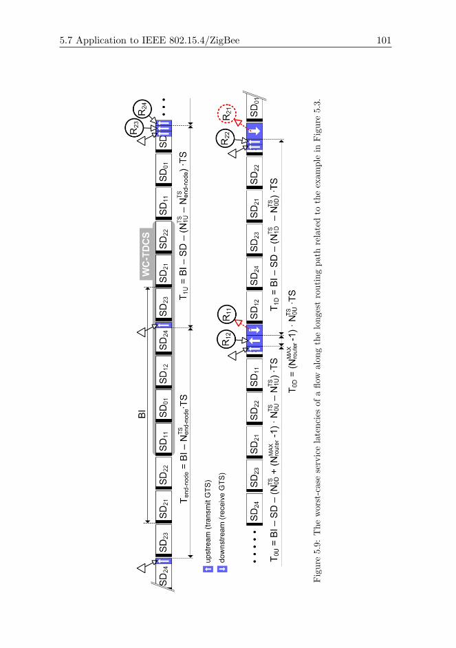
5.7 Application to IEEE 802.15.4/ZigBee 101
Fig
ure
5.9:
The
wor
st-c
ase
serv
ice
late
ncie
sof
aflo
wal
ong
the
long
est
rout
ing
path
rela
ted
toth
eex
ampl
ein
Fig
ure
5.3.

102 Chapter 5 Dimensioning and worst-case analysis of cluster-tree WSNs
According to Figure 5.9, the worst-case service latency guaranteed to aflow over an upstream data link at a given depth is expressed as:
– the latency guaranteed by a router to its end-node:
Tend−node = BI−NTSend−node · TS
– the latency guaranteed by a router at depth i to a child router at depthi+ 1, for ∀i, 0 < i < H:
TiU = BI− SD−(NTS
iU −NTS(i+1)U
)· TS
– the latency guaranteed by the router at depth 0 to the child router atdepth 1:
T0U = BI− SD−(NTS
0D +(NMAX
router − 1)·NTS
0U −NTS1U
)· TS
On the other hand, the worst-case service latency guaranteed to a flowover a downstream data link at a given depth is expressed as:
– the latency guaranteed by a router at depth 0 to the child router atdepth 1 (priority rule, Section 5.4.3):
T0D =(NMAX
router − 1)·NTS
0U · TS
– the latency guaranteed by a router at depth i to the child router atdepth i+ 1, for ∀i, 0 < i < Hsink:
TiD = BI− SD−(NTS
iD −NTS(i−1)D
)· TS
5.7.3 IEEE 802.15.4/ZigBee cluster-tree WSN setup
The experimental scenario considers a simple cluster-tree WSN correspondingto the configuration where H = 2, NMAX
end−node = 1, NMAXrouter = 2. For the sake
of simplicity, only end-nodes are equipped with sensing capability (i.e. ω = 0)and generate sensory data bounded by the arrival curve αdata. The SO isassumed to be equal to 4, which is the minimum value that is possible to usewithout resulting into synchronization problem [70], using open-ZB protocolstack [71] over TinyOS [72] and MICAz/TelosB motes. This constraint resultsfrom the lack of task prioritization and non-preemptive behaviour of theTinyOS operating system. According to Eq. (5.36), the total number ofrouters is equal to 7. Hence, BO must be set such that at least seven SDswith SO = 4 can fit inside the BI without overlapping.
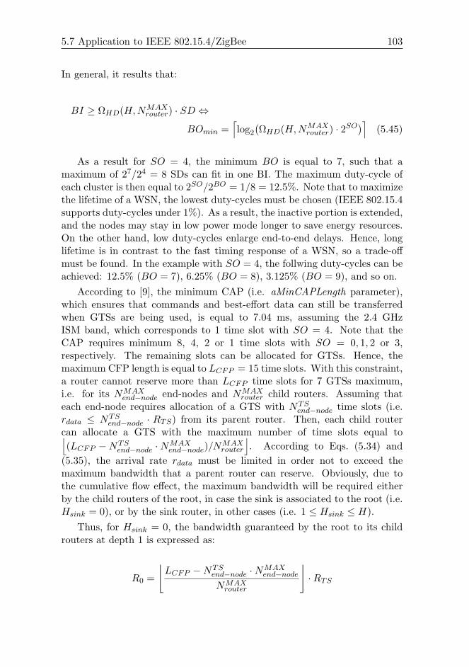
5.7 Application to IEEE 802.15.4/ZigBee 103
In general, it results that:
BI ≥ ΩHD(H,NMAXrouter) · SD ⇔
BOmin =⌈log2
(ΩHD(H,NMAX
router) · 2SO)⌉ (5.45)
As a result for SO = 4, the minimum BO is equal to 7, such that amaximum of 27/24 = 8 SDs can fit in one BI. The maximum duty-cycle ofeach cluster is then equal to 2SO/2BO = 1/8 = 12.5%. Note that to maximizethe lifetime of a WSN, the lowest duty-cycles must be chosen (IEEE 802.15.4supports duty-cycles under 1%). As a result, the inactive portion is extended,and the nodes may stay in low power mode longer to save energy resources.On the other hand, low duty-cycles enlarge end-to-end delays. Hence, longlifetime is in contrast to the fast timing response of a WSN, so a trade-offmust be found. In the example with SO = 4, the follwing duty-cycles can beachieved: 12.5% (BO = 7), 6.25% (BO = 8), 3.125% (BO = 9), and so on.
According to [9], the minimum CAP (i.e. aMinCAPLength parameter),which ensures that commands and best-effort data can still be transferredwhen GTSs are being used, is equal to 7.04 ms, assuming the 2.4 GHzISM band, which corresponds to 1 time slot with SO = 4. Note that theCAP requires minimum 8, 4, 2 or 1 time slots with SO = 0, 1, 2 or 3,respectively. The remaining slots can be allocated for GTSs. Hence, themaximum CFP length is equal to LCFP = 15 time slots. With this constraint,a router cannot reserve more than LCFP time slots for 7 GTSs maximum,i.e. for its NMAX
end−node end-nodes and NMAXrouter child routers. Assuming that
each end-node requires allocation of a GTS with NTSend−node time slots (i.e.
rdata ≤ NTSend−node · RTS) from its parent router. Then, each child router
can allocate a GTS with the maximum number of time slots equal to⌊(LCFP −NTS
end−node ·NMAXend−node)/N
MAXrouter
⌋. According to Eqs. (5.34) and
(5.35), the arrival rate rdata must be limited in order not to exceed themaximum bandwidth that a parent router can reserve. Obviously, due tothe cumulative flow effect, the maximum bandwidth will be required eitherby the child routers of the root, in case the sink is associated to the root (i.e.Hsink = 0), or by the sink router, in other cases (i.e. 1 ≤ Hsink ≤ H).
Thus, for Hsink = 0, the bandwidth guaranteed by the root to its childrouters at depth 1 is expressed as:
R0 =
⌊LCFP −NTS
end−node ·NMAXend−node
NMAXrouter
⌋·RTS

104 Chapter 5 Dimensioning and worst-case analysis of cluster-tree WSNs
As a result, applying Eq. (5.34) will lead to the maximum arrival rate ofthe sensory data:
rMAXdata =
⌊LCFP −NTS
end−node ·NMAXend−node
NMAXrouter
⌋·
RTS(∑H−1j=0 (NMAX
router)j)·(NMAX
end−node + ω) (5.46)
for Hsink = 0.On the other hand, for 1 ≤ Hsink ≤ H, the corresponding link bandwidth
guaranteed by the parent router at depth (Hsink − 1) to the sink router atdepth Hsink is equal to:
R(Hsink−1) =
⌊LCFP −NTS
end−node ·NMAXend−node
NMAXrouter
⌋·RTS
As a result, applying Eq. (5.35) will lead to the maximum arrival rate ofthe sensory data:
rMAXdata =
⌊LCFP −NTS
end−node ·NMAXend−node
NMAXrouter
⌋·
RTS(∑Hsink−1j=0 (NMAX
router)H−j)·(NMAX
end−node + ω) (5.47)
for ∀Hsink, 1 ≤ Hsink ≤ H.The average arrival rate rdata of sensory data must be lower than rMAX
data
in any case. The value of burst bdata is selected according to the burstinessof sensory data.
5.8 Performance evaluation
This section compares the analytical results based on Network Calculus withthe experimental results obtained through the use of IEEE 802.15.4/ZigBeetechnologies. The analytical results are computed using a Matlab tool [73],and the experimental results are obtained using a test-bed based on theTelosB motes [14].
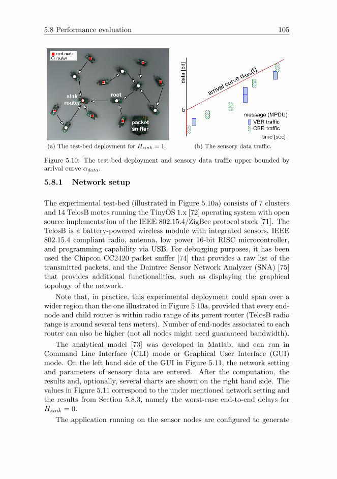
5.8 Performance evaluation 105
(a) The test-bed deployment for Hsink = 1. (b) The sensory data traffic.
Figure 5.10: The test-bed deployment and sensory data traffic upper bounded byarrival curve αdata.
5.8.1 Network setup
The experimental test-bed (illustrated in Figure 5.10a) consists of 7 clustersand 14 TelosB motes running the TinyOS 1.x [72] operating system with opensource implementation of the IEEE 802.15.4/ZigBee protocol stack [71]. TheTelosB is a battery-powered wireless module with integrated sensors, IEEE802.15.4 compliant radio, antenna, low power 16-bit RISC microcontroller,and programming capability via USB. For debugging purposes, it has beenused the Chipcon CC2420 packet sniffer [74] that provides a raw list of thetransmitted packets, and the Daintree Sensor Network Analyzer (SNA) [75]that provides additional functionalities, such as displaying the graphicaltopology of the network.
Note that, in practice, this experimental deployment could span over awider region than the one illustrated in Figure 5.10a, provided that every end-node and child router is within radio range of its parent router (TelosB radiorange is around several tens meters). Number of end-nodes associated to eachrouter can also be higher (not all nodes might need guaranteed bandwidth).
The analytical model [73] was developed in Matlab, and can run inCommand Line Interface (CLI) mode or Graphical User Interface (GUI)mode. On the left hand side of the GUI in Figure 5.11, the network settingand parameters of sensory data are entered. After the computation, theresults and, optionally, several charts are shown on the right hand side. Thevalues in Figure 5.11 correspond to the under mentioned network setting andthe results from Section 5.8.3, namely the worst-case end-to-end delays forHsink = 0.
The application running on the sensor nodes are configured to generate

106 Chapter 5 Dimensioning and worst-case analysis of cluster-tree WSNs
Figure 5.11: The GUI of the Matlab analytical model.
5 bytes at the data payload of every message. Hence, the maximum size ofthe MAC frame is equal to MPDUmax = 192 bits (i.e. MAC Header = 72bits, FCS = 16 bits, Network Header = 64 bits, and Data Payload = 40 bits)assuming only destination PAN identifier and both source and destinationaddresses are present. Note that all nodes in the WSN have unique 16-bit short addresses assigned by the PAN Coordinator during the associationprocess.
TinyOS 1.x flushes the reception buffer of the radio transceiver afterprocessing the first arriving frame. Thus, the frames that arrive duringthe processing time of the first frame are discarded. This problem has beenalready reported and fixed in TinyOS 2.x. Since the proposed implementationof IEEE 802.15.4/ZigBee protocol stack was built over TinyOS 1.x, theaforementioned problem is overcame by setting the inter-frame spacing (IFS)time (i.e. time between two consecutive frames) such that no frame arrivesduring the frame processing time. A value of IFS equal to 3.07 ms wasmeasured.
According to Eq. (5.43), the bandwidth guaranteed by one time slotfor SO = 4 is equal to 3.125 kbps with 100% duty-cycle. Hence, in theexperimental scenario with a 12.5% duty-cycle (i.e. BO = BOmin = 7), theguaranteed bandwidth of one time slot is equal to RTS = 3.125 · 0.125 =0.3906 kbps. Let us assume NTS
end−node = 1. Then, according to Eqs. (5.46)and (5.47), the maximum arrival rates of the sensory data are obtained as
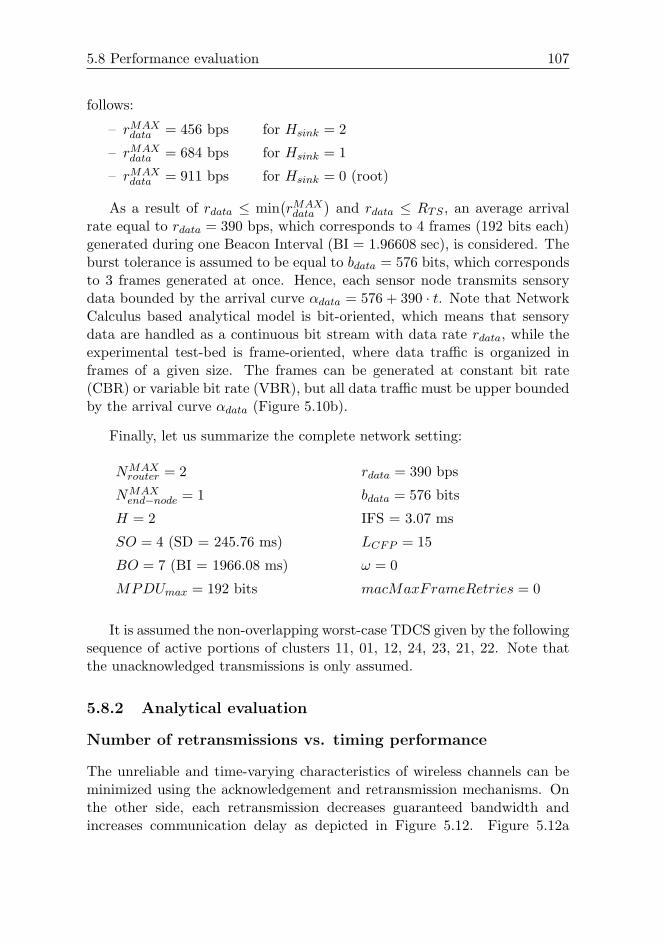
5.8 Performance evaluation 107
follows:
– rMAXdata = 456 bps for Hsink = 2
– rMAXdata = 684 bps for Hsink = 1
– rMAXdata = 911 bps for Hsink = 0 (root)
As a result of rdata ≤ min(rMAXdata
)and rdata ≤ RTS , an average arrival
rate equal to rdata = 390 bps, which corresponds to 4 frames (192 bits each)generated during one Beacon Interval (BI = 1.96608 sec), is considered. Theburst tolerance is assumed to be equal to bdata = 576 bits, which correspondsto 3 frames generated at once. Hence, each sensor node transmits sensorydata bounded by the arrival curve αdata = 576 + 390 · t. Note that NetworkCalculus based analytical model is bit-oriented, which means that sensorydata are handled as a continuous bit stream with data rate rdata, while theexperimental test-bed is frame-oriented, where data traffic is organized inframes of a given size. The frames can be generated at constant bit rate(CBR) or variable bit rate (VBR), but all data traffic must be upper boundedby the arrival curve αdata (Figure 5.10b).
Finally, let us summarize the complete network setting:
NMAXrouter = 2 rdata = 390 bps
NMAXend−node = 1 bdata = 576 bits
H = 2 IFS = 3.07 ms
SO = 4 (SD = 245.76 ms) LCFP = 15
BO = 7 (BI = 1966.08 ms) ω = 0
MPDUmax = 192 bits macMaxFrameRetries = 0
It is assumed the non-overlapping worst-case TDCS given by the followingsequence of active portions of clusters 11, 01, 12, 24, 23, 21, 22. Note thatthe unacknowledged transmissions is only assumed.
5.8.2 Analytical evaluation
Number of retransmissions vs. timing performance
The unreliable and time-varying characteristics of wireless channels can beminimized using the acknowledgement and retransmission mechanisms. Onthe other side, each retransmission decreases guaranteed bandwidth andincreases communication delay as depicted in Figure 5.12. Figure 5.12a
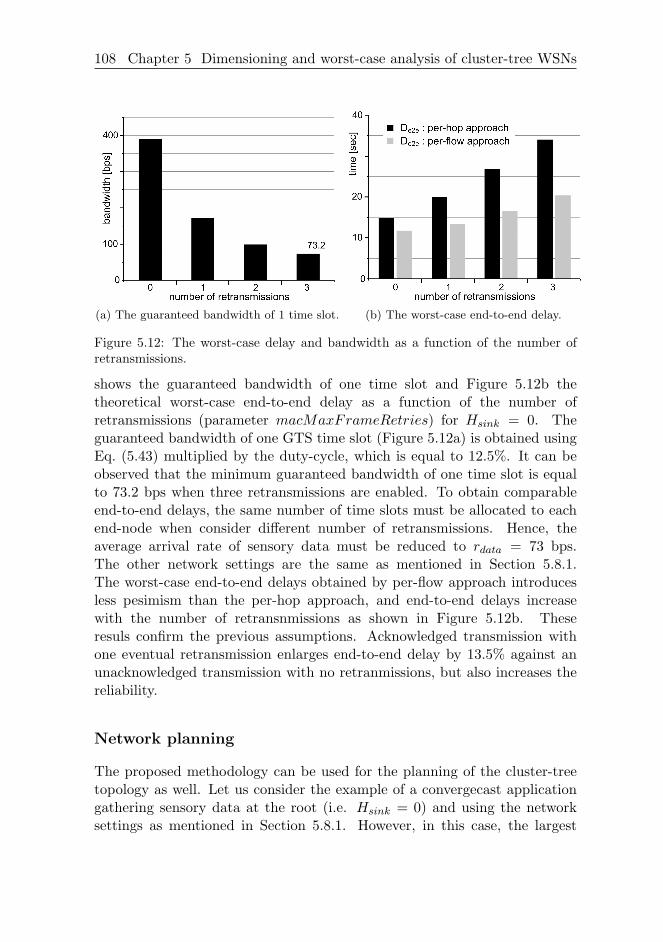
108 Chapter 5 Dimensioning and worst-case analysis of cluster-tree WSNs
(a) The guaranteed bandwidth of 1 time slot. (b) The worst-case end-to-end delay.
Figure 5.12: The worst-case delay and bandwidth as a function of the number ofretransmissions.
shows the guaranteed bandwidth of one time slot and Figure 5.12b thetheoretical worst-case end-to-end delay as a function of the number ofretransmissions (parameter macMaxFrameRetries) for Hsink = 0. Theguaranteed bandwidth of one GTS time slot (Figure 5.12a) is obtained usingEq. (5.43) multiplied by the duty-cycle, which is equal to 12.5%. It can beobserved that the minimum guaranteed bandwidth of one time slot is equalto 73.2 bps when three retransmissions are enabled. To obtain comparableend-to-end delays, the same number of time slots must be allocated to eachend-node when consider different number of retransmissions. Hence, theaverage arrival rate of sensory data must be reduced to rdata = 73 bps.The other network settings are the same as mentioned in Section 5.8.1.The worst-case end-to-end delays obtained by per-flow approach introducesless pesimism than the per-hop approach, and end-to-end delays increasewith the number of retransnmissions as shown in Figure 5.12b. Theseresuls confirm the previous assumptions. Acknowledged transmission withone eventual retransmission enlarges end-to-end delay by 13.5% against anunacknowledged transmission with no retranmissions, but also increases thereliability.
Network planning
The proposed methodology can be used for the planning of the cluster-treetopology as well. Let us consider the example of a convergecast applicationgathering sensory data at the root (i.e. Hsink = 0) and using the networksettings as mentioned in Section 5.8.1. However, in this case, the largest
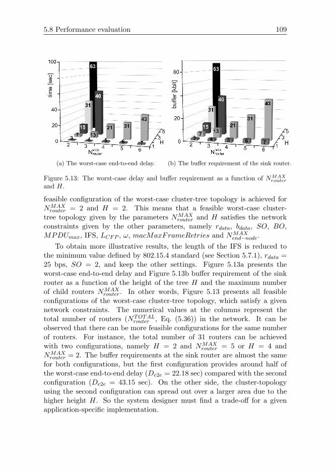
5.8 Performance evaluation 109
(a) The worst-case end-to-end delay. (b) The buffer requirement of the sink router.
Figure 5.13: The worst-case delay and buffer requirement as a function of NMAXrouter
and H.
feasible configuration of the worst-case cluster-tree topology is achieved forNMAX
router = 2 and H = 2. This means that a feasible worst-case cluster-tree topology given by the parameters NMAX
router and H satisfies the networkconstraints given by the other parameters, namely rdata, bdata, SO, BO,MPDUmax, IFS, LCFP , ω, macMaxFrameRetries and NMAX
end−node.To obtain more illustrative results, the length of the IFS is reduced to
the minimum value defined by 802.15.4 standard (see Section 5.7.1), rdata =25 bps, SO = 2, and keep the other settings. Figure 5.13a presents theworst-case end-to-end delay and Figure 5.13b buffer requirement of the sinkrouter as a function of the height of the tree H and the maximum numberof child routers NMAX
router. In other words, Figure 5.13 presents all feasibleconfigurations of the worst-case cluster-tree topology, which satisfy a givennetwork constraints. The numerical values at the columns represent thetotal number of routers (NTOTAL
router , Eq. (5.36)) in the network. It can beobserved that there can be more feasible configurations for the same numberof routers. For instance, the total number of 31 routers can be achievedwith two configurations, namely H = 2 and NMAX
router = 5 or H = 4 andNMAX
router = 2. The buffer requirements at the sink router are almost the samefor both configurations, but the first configuration provides around half ofthe worst-case end-to-end delay (De2e = 22.18 sec) compared with the secondconfiguration (De2e = 43.15 sec). On the other side, the cluster-topologyusing the second configuration can spread out over a larger area due to thehigher height H. So the system designer must find a trade-off for a givenapplication-specific implementation.
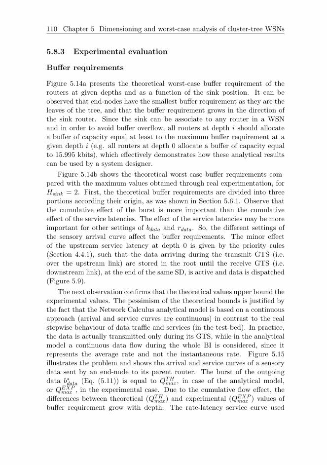
110 Chapter 5 Dimensioning and worst-case analysis of cluster-tree WSNs
5.8.3 Experimental evaluation
Buffer requirements
Figure 5.14a presents the theoretical worst-case buffer requirement of therouters at given depths and as a function of the sink position. It can beobserved that end-nodes have the smallest buffer requirement as they are theleaves of the tree, and that the buffer requirement grows in the direction ofthe sink router. Since the sink can be associate to any router in a WSNand in order to avoid buffer overflow, all routers at depth i should allocatea buffer of capacity equal at least to the maximum buffer requirement at agiven depth i (e.g. all routers at depth 0 allocate a buffer of capacity equalto 15.995 kbits), which effectively demonstrates how these analytical resultscan be used by a system designer.
Figure 5.14b shows the theoretical worst-case buffer requirements com-pared with the maximum values obtained through real experimentation, forHsink = 2. First, the theoretical buffer requirements are divided into threeportions according their origin, as was shown in Section 5.6.1. Observe thatthe cumulative effect of the burst is more important than the cumulativeeffect of the service latencies. The effect of the service latencies may be moreimportant for other settings of bdata and rdata. So, the different settings ofthe sensory arrival curve affect the buffer requirements. The minor effectof the upstream service latency at depth 0 is given by the priority rules(Section 4.4.1), such that the data arriving during the transmit GTS (i.e.over the upstream link) are stored in the root until the receive GTS (i.e.downstream link), at the end of the same SD, is active and data is dispatched(Figure 5.9).
The next observation confirms that the theoretical values upper bound theexperimental values. The pessimism of the theoretical bounds is justified bythe fact that the Network Calculus analytical model is based on a continuousapproach (arrival and service curves are continuous) in contrast to the realstepwise behaviour of data traffic and services (in the test-bed). In practice,the data is actually transmitted only during its GTS, while in the analyticalmodel a continuous data flow during the whole BI is considered, since itrepresents the average rate and not the instantaneous rate. Figure 5.15illustrates the problem and shows the arrival and service curves of a sensorydata sent by an end-node to its parent router. The burst of the outgoingdata b∗data (Eq. (5.11)) is equal to QTH
max, in case of the analytical model,or QEXP
max , in the experimental case. Due to the cumulative flow effect, thedifferences between theoretical (QTH
max) and experimental (QEXPmax ) values of
buffer requirement grow with depth. The rate-latency service curve used
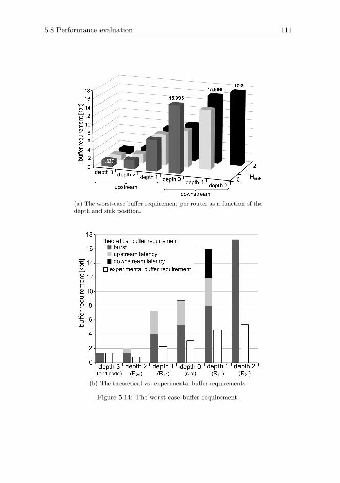
5.8 Performance evaluation 111
(a) The worst-case buffer requirement per router as a function of thedepth and sink position.
(b) The theoretical vs. experimental buffer requirements.
Figure 5.14: The worst-case buffer requirement.
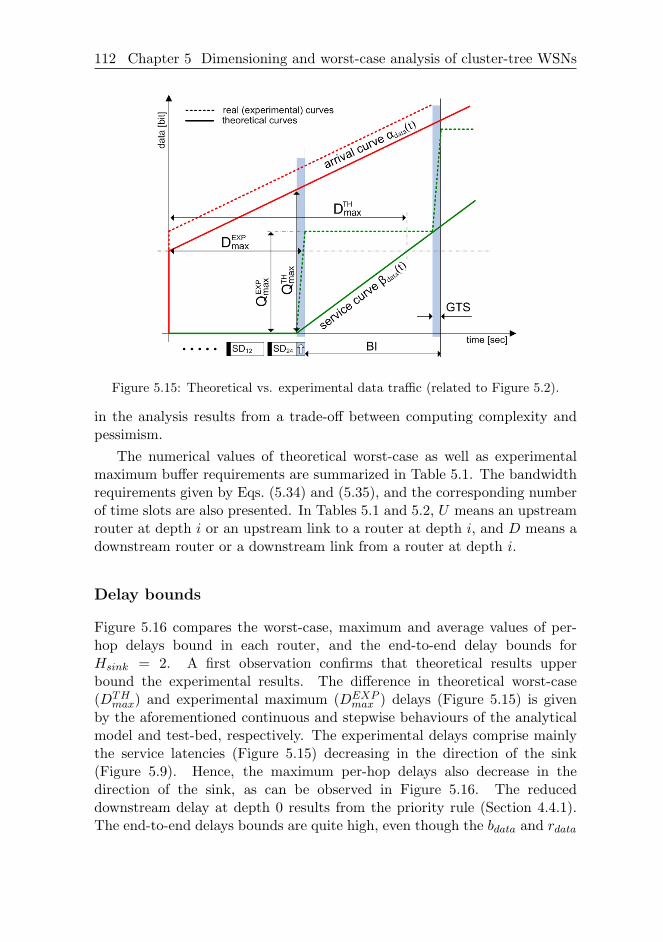
112 Chapter 5 Dimensioning and worst-case analysis of cluster-tree WSNs
Figure 5.15: Theoretical vs. experimental data traffic (related to Figure 5.2).
in the analysis results from a trade-off between computing complexity andpessimism.
The numerical values of theoretical worst-case as well as experimentalmaximum buffer requirements are summarized in Table 5.1. The bandwidthrequirements given by Eqs. (5.34) and (5.35), and the corresponding numberof time slots are also presented. In Tables 5.1 and 5.2, U means an upstreamrouter at depth i or an upstream link to a router at depth i, and D means adownstream router or a downstream link from a router at depth i.
Delay bounds
Figure 5.16 compares the worst-case, maximum and average values of per-hop delays bound in each router, and the end-to-end delay bounds forHsink = 2. A first observation confirms that theoretical results upperbound the experimental results. The difference in theoretical worst-case(DTH
max) and experimental maximum (DEXPmax ) delays (Figure 5.15) is given
by the aforementioned continuous and stepwise behaviours of the analyticalmodel and test-bed, respectively. The experimental delays comprise mainlythe service latencies (Figure 5.15) decreasing in the direction of the sink(Figure 5.9). Hence, the maximum per-hop delays also decrease in thedirection of the sink, as can be observed in Figure 5.16. The reduceddownstream delay at depth 0 results from the priority rule (Section 4.4.1).The end-to-end delays bounds are quite high, even though the bdata and rdata
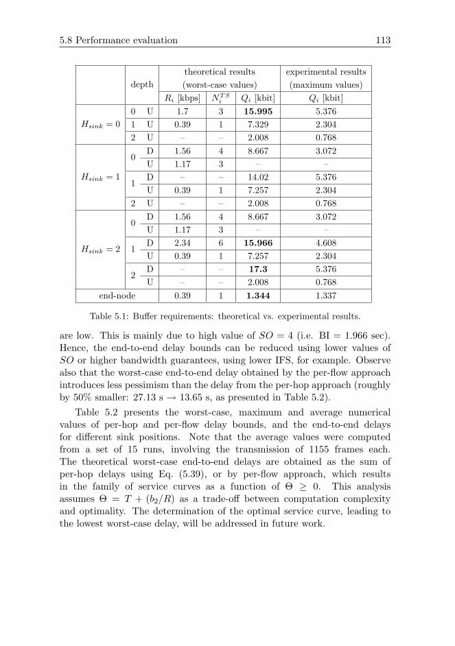
5.8 Performance evaluation 113
depththeoretical results experimental results(worst-case values) (maximum values)
Ri [kbps] NTSi Qi [kbit] Qi [kbit]
Hsink = 00 U 1.7 3 15.995 5.3761 U 0.39 1 7.329 2.3042 U – – 2.008 0.768
Hsink = 1
0D 1.56 4 8.667 3.072U 1.17 3 – –
1D – – 14.02 5.376U 0.39 1 7.257 2.304
2 U – – 2.008 0.768
Hsink = 2
0D 1.56 4 8.667 3.072U 1.17 3 – –
1D 2.34 6 15.966 4.608U 0.39 1 7.257 2.304
2D – – 17.3 5.376U – – 2.008 0.768
end-node 0.39 1 1.344 1.337
Table 5.1: Buffer requirements: theoretical vs. experimental results.
are low. This is mainly due to high value of SO = 4 (i.e. BI = 1.966 sec).Hence, the end-to-end delay bounds can be reduced using lower values ofSO or higher bandwidth guarantees, using lower IFS, for example. Observealso that the worst-case end-to-end delay obtained by the per-flow approachintroduces less pessimism than the delay from the per-hop approach (roughlyby 50% smaller: 27.13 s → 13.65 s, as presented in Table 5.2).
Table 5.2 presents the worst-case, maximum and average numericalvalues of per-hop and per-flow delay bounds, and the end-to-end delaysfor different sink positions. Note that the average values were computedfrom a set of 15 runs, involving the transmission of 1155 frames each.The theoretical worst-case end-to-end delays are obtained as the sum ofper-hop delays using Eq. (5.39), or by per-flow approach, which resultsin the family of service curves as a function of Θ ≥ 0. This analysisassumes Θ = T + (b2/R) as a trade-off between computation complexityand optimality. The determination of the optimal service curve, leading tothe lowest worst-case delay, will be addressed in future work.
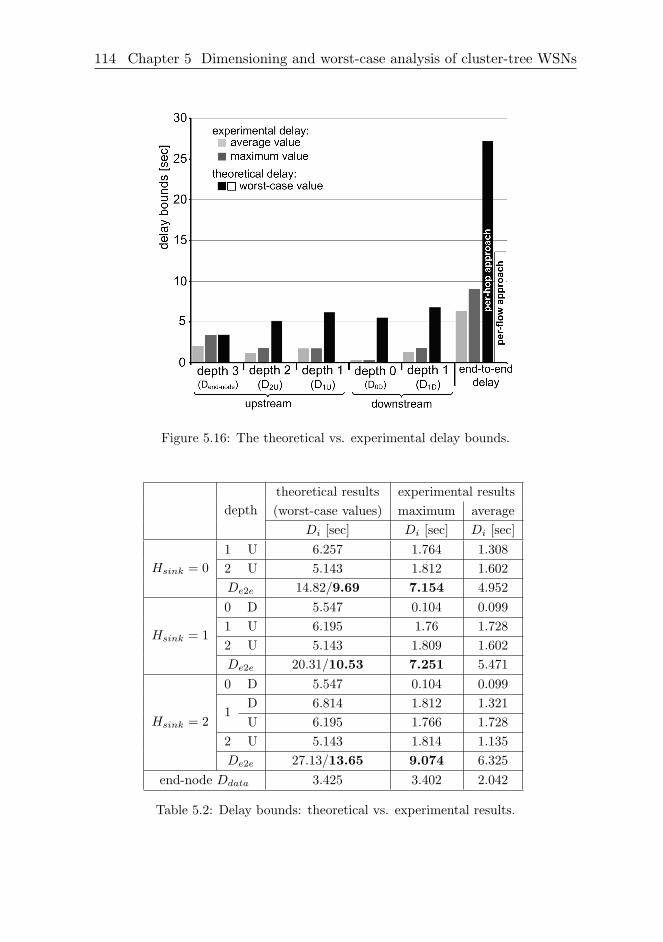
114 Chapter 5 Dimensioning and worst-case analysis of cluster-tree WSNs
Figure 5.16: The theoretical vs. experimental delay bounds.
depththeoretical results experimental results(worst-case values) maximum average
Di [sec] Di [sec] Di [sec]
Hsink = 01 U 6.257 1.764 1.3082 U 5.143 1.812 1.602De2e 14.82/9.69 7.154 4.952
Hsink = 1
0 D 5.547 0.104 0.0991 U 6.195 1.76 1.7282 U 5.143 1.809 1.602De2e 20.31/10.53 7.251 5.471
Hsink = 2
0 D 5.547 0.104 0.099
1D 6.814 1.812 1.321U 6.195 1.766 1.728
2 U 5.143 1.814 1.135De2e 27.13/13.65 9.074 6.325
end-node Ddata 3.425 3.402 2.042
Table 5.2: Delay bounds: theoretical vs. experimental results.
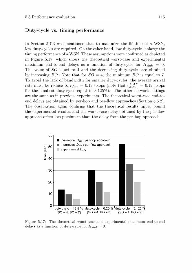
5.8 Performance evaluation 115
Duty-cycle vs. timing performance
In Section 5.7.3 was mentioned that to maximize the lifetime of a WSN,low duty-cycles are required. On the other hand, low duty-cycles enlarge thetiming performance of a WSN. These assumptions were confirmed as depictedin Figure 5.17, which shows the theoretical worst-case and experimentalmaximum end-to-end delays as a function of duty-cycle for Hsink = 0.The value of SO is set to 4 and the decreasing duty-cycles are obtainedby increasing BO. Note that for SO = 4, the minimum BO is equal to 7.To avoid the lack of bandwidth for smaller duty-cycles, the average arrivalrate must be reduce to rdata = 0.190 kbps (note that rMAX
data = 0.195 kbpsfor the smallest duty-cycle equal to 3.125%). The other network settingsare the same as in previous experiments. The theoretical worst-case end-to-end delays are obtained by per-hop and per-flow approaches (Section 5.6.2).The observation again confirms that the theoretical results upper boundthe experimental results, and the worst-case delay obtained by the per-flowapproach offers less pessimism than the delay from the per-hop approach.
Figure 5.17: The theoretical worst-case and experimental maximum end-to-enddelays as a function of duty-cycle for Hsink = 0.

116 Chapter 5 Dimensioning and worst-case analysis of cluster-tree WSNs
5.9 Discussion on mobility support
This section outlines several issues related to how to support the sink mobilityin a cluster-tree WSN.
5.9.1 Adapting the logical topology
All network nodes (i.e. routers and end-nodes) are assumed to be static;note that even the sink router is static - only the sink entity can be mobile.Considering the mobile sink behaviour, the logical topology has to be adaptedto allow sensory data to reach the new sink location. Two approachesto mobile sink behaviour are assumed: topology update (Figure 5.18a),applicable to the cases where the sink moves more frequently (i.e. in acontinuous fashion), and topology rebuilding (Figure 5.18b), applicable tothe cases where the sink changes location less frequently (sporadically).Generally, the topology update approach should be chosen when the networkinaccessibility time resulting from the topology rebuilding is greater thanthe maximum time between two consecutive sink movements (i.e. twoconsecutive sink associations with different sink routers).
The topology update
When the sink moves very frequently, it might be more adequate to keep thelogical topology unchanged (the same original root and network deployment).Hence, the path of data flows in the direction of the sink has to be updatedaccordingly (dubbed topology update). The length of this updated path isequal to the number of hops between the previous and current sink routerpositions. In the worst-case, when the sink moves between two farthestrouters of different sub-trees of the root, the length of the update pathbecomes twice the height of the cluster-tree. Thus, the network inaccessibilitytime will depend on the length of the update path and on the TDCS. In case ofthe worst-case TDCS, the inaccessibility time is expressed as the period of theWC-TDCS multiplied by the length of the update path. This inaccessibilitytime is much smaller than the network inaccessibility time resulting from thetopology rebuilding (see next), and also the energy consumption during thetopology update is expected to be lower. On the other hand, the resourcerequirements (i.e. the resources guaranteed along the longest data path) inthe updated topology are higher as compared to the rebuilt topology. Itresults in a balanced topology with unbalanced load requiring higher energyconsumption and higher end-to-end delay bounds.
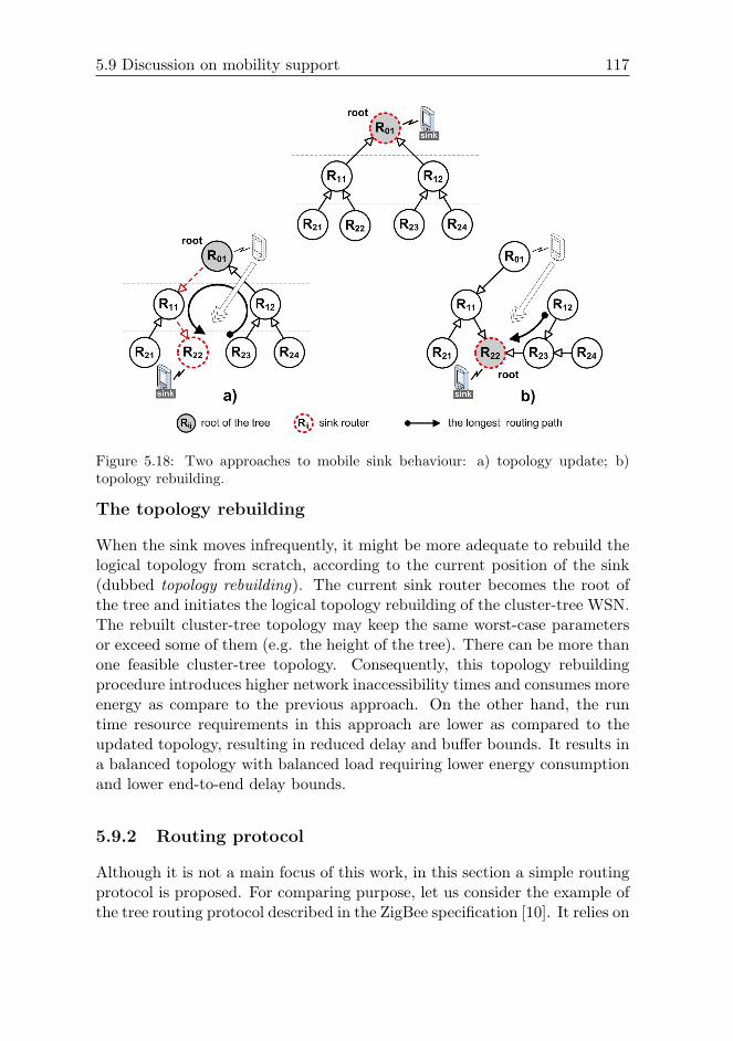
5.9 Discussion on mobility support 117
Figure 5.18: Two approaches to mobile sink behaviour: a) topology update; b)topology rebuilding.
The topology rebuilding
When the sink moves infrequently, it might be more adequate to rebuild thelogical topology from scratch, according to the current position of the sink(dubbed topology rebuilding). The current sink router becomes the root ofthe tree and initiates the logical topology rebuilding of the cluster-tree WSN.The rebuilt cluster-tree topology may keep the same worst-case parametersor exceed some of them (e.g. the height of the tree). There can be more thanone feasible cluster-tree topology. Consequently, this topology rebuildingprocedure introduces higher network inaccessibility times and consumes moreenergy as compare to the previous approach. On the other hand, the runtime resource requirements in this approach are lower as compared to theupdated topology, resulting in reduced delay and buffer bounds. It results ina balanced topology with balanced load requiring lower energy consumptionand lower end-to-end delay bounds.
5.9.2 Routing protocol
Although it is not a main focus of this work, in this section a simple routingprotocol is proposed. For comparing purpose, let us consider the example ofthe tree routing protocol described in the ZigBee specification [10]. It relies on
118 Chapter 5 Dimensioning and worst-case analysis of cluster-tree WSNs
a distributed address assignment mechanism that provides a finite sub-blockof hierarchical unique network addresses to each parent router. Since the treerouting algorithm is address-based, each node requires assignment of a uniquenetwork address from its parent router. If a parent router lacks availableaddresses, the address assignment mechanism imposes address redistribution,causing some network inaccessibility time. Conversely, the proposed routingprotocol reduces the inaccessibility time and simplifies the joining of newnodes. The messages are routed locally, from cluster to cluster, until reachingthe sink. Thus, the node’s address must be unique only between the adjacentclusters, and a joining node is assigned an arbitrary unused address. On theother hand, the proposed protocol is only suitable for a cluster-tree WSNwhere all data flows are routed to the sink.
Routing algorithm
The algorithm assumes that each router is assigned an address, prior to run-time, which is unique with respect to its adjacent clusters. New router’sparameter, called next hop to sink (referred to as NH2S hereafter), isdefined. The value of this parameter is equal to the address of the nextrouter on the path towards the current sink location; all incoming trafficis forwarded to this direction. In case of the sink router, this parameter isequal to its own address. After the cluster-tree topology is built up (or rebuiltin case of the topology rebuilding approach), the NH2S parameter of eachrouter contains the address of its parent router (in the cluster-tree hierarchy)or its own address in case of root, and the sink is initially associated to theroot.
Route update algorithm
In case of the topology update approach, the path of data flows in thedirection of the sink has to be updated, to enable data flows to be correctlyrouted to the sink. The route update algorithm is proposed as a part ofthe routing protocol that tracks the frequently moving sink and updates theNH2S parameters of the relevant routers.
This algorithm is illustrated in Figure 5.19 and is described next. Let usassume that the sink has moved (from R01, in Figure 5.19a) and associated toanother router (R22). The current sink router must notify all routers alongthe update path to the previous sink router position (R01). The routersalong the update path (R22, R11 and R01) update their NH2S parameters.On the contrary, the routers out of the update path keep the same NH2S
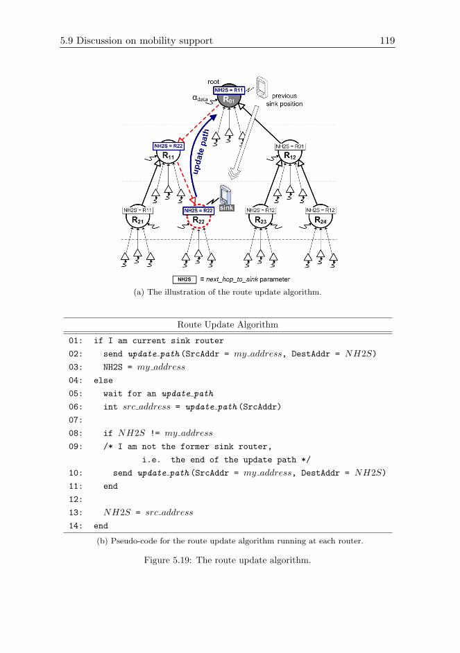
5.9 Discussion on mobility support 119
(a) The illustration of the route update algorithm.
Route Update Algorithm
01: if I am current sink router
02: send update path (SrcAddr = my address, DestAddr = NH2S)03: NH2S = my address
04: else
05: wait for an update path
06: int src address = update path (SrcAddr)
07:
08: if NH2S != my address
09: /* I am not the former sink router,
i.e. the end of the update path */
10: send update path (SrcAddr = my address, DestAddr = NH2S)11: end
12:
13: NH2S = src address
14: end
(b) Pseudo-code for the route update algorithm running at each router.
Figure 5.19: The route update algorithm.
120 Chapter 5 Dimensioning and worst-case analysis of cluster-tree WSNs
values. First, the current sink router (R22) sends an update path messageto its next hop to sink router (R11) and then updates its NH2S parameterwith its own address. After receiving this update path message, the nextrouter (R11) on the update path sends another update path message to itsnext hop to sink router (R01) and then updates its NH2S parameter withthe source address embedded in the received update path message (R22).This procedure is repeated router by router until reaching the former sinkrouter (i.e. a router which NH2S parameter is equal to its own address -R01). The former sink router (R01) does not send a new update path messageand only updates its NH2S variable with the source address of the receivedupdate path message.
During the update process, just some links between correspondent routersare reversed, thus not impacting the entire network (involving the minimumnumber of routers/messages), so normal network operation can quickly beresumed. As a result, this algorithm requires a minimum amount of control-related traffic and reduces network inaccessibility times (the computation ofthese inaccessibility times is out of the context of this work).
5.10 Conclusions
Modelling the fundamental performance limits of Wireless Sensor Networks(WSNs) is of paramount importance to understand their behaviour underthe worst-case conditions and to make the appropriate design choices.In that direction this chapter contributes with a methodology based onNetwork Calculus, which enables quick and efficient worst-case analysis anddimensioning of static or even dynamically changing cluster-tree WSNs wherethe data sink can either be static or mobile, i.e. can be associated toany router in the WSN. The proposed analytical methodology (closed-formrecurrent expressions) enables to guarantee the routers’ buffer size to avoidbuffer overflows and to minimize clusters’ duty-cycle (maximizing nodes’lifetime) still satisfying that messages’ deadlines are met.
The chapter also shows how to instantiate the generic methodology inIEEE 802.15.4/ZigBee, which are promising technologies for WSN applica-tions. Finally, based on the Commercial-Off-The-Shelf (COTS) technolo-gies, namely TelosB motes [14] running open-ZB protocol stack [71] overTinyOS [72], a multiple cluster test-bed has been configured. This test-bedenabled to assess the validity and pessimism of the worst-case theoreticalresults (buffer requirements and message end-to-end delays), by comparingthese to the maximum and average values measured in the experiments. The

5.A Table of symbols 121
results confirm that the theoretical values upper bound the experimentalvalues, the buffer requirements grow in the direction of the sink router,and the end-to-end delays increase with number of retransmissions. Theobservation also shows that the worst-case end-to-end delay obtained bythe per-flow approach offers less pessimism than the delay from the per-hop approach (roughly by 50%). Using the proposed methodology for theplanning of the cluster-tree networks is demonstrated by the illustrativeexample.
The future work includes improving the current methodology to encom-pass clusters operating at different duty-cycles and to provide a model thatenables real-time control actions, i.e. the sink assuming the role of controllingsensor/actuator nodes.
APPENDIX
5.A Table of symbols
The following table reports the symbols that are used through the Chapter 5,along with their definition.
Symbol Definition
R(t) input cumulative function
R∗(t) output cumulative function
α(t) arrival curve
β(t) guaranteed service curve
α∗(t) output bound constraining the output function R∗(t)
Dmax delay bound
Qmax backlog bound
min-plus deconvolution
⊗ min-plus convolution
βeq1 (t,Θ) equivalent service curve for flow 1
1expr 1expr is equal to 1 if expr is true, and 0 otherwise.
(x)+ (x)+ = max(0, x)
αb,r(t) affine arrival curve with rate r and burst size b

122 Chapter 5 Dimensioning and worst-case analysis of cluster-tree WSNs
βR,T (t) rate-latency service curve with rate R and latency T
H height of the tree
NMAXend−node maximum number of child end-nodes
NMAXrouter maximum number of child routers
Hsink maximum depth of the sink router
βend−node(t) rate-latency service curve guaranteed to end-nodes
αdata(t) affine arrival curve constraining sensory data
αi(t) affine arrival curve constraining the input function R(t)
of a router at a depth i
α∗i (t) output bound constraining the output function R∗(t)
of a router at a depth i
βi(t) rate-latency service curve guaranteed by a router at depth i
ω binary variable which is equal to 1 if routers have sensing
capabilities; otherwise ω is equal to 0
QiU the required buffer size of an upstream router at a depth i
DiU delay bound between a child router at depth i
and its parent router at depth i− 1
DiD delay bound between a parent router at depth i
and its child router at depth i+ 1
De2e the worst-case end-to-end delay
Table 5.3: Table of symbols.
Chapter 6
Conclusions
This thesis addresses several problems and open research issues in the areaof design and performance evaluation of the cluster-tree Wireless SensorNetworks (WSN) focusing on the energy efficient and real-time behaviour.The proposed methodologies are instantiated in the IEEE 802.15.4/ZigBeebeacon-enabled cluster-tree WSNs, as an illustrative example that confirmsthe applicability of general approach to specific protocols. The IEEE802.15.4/ZigBee protocols, which are the leading technologies for WSNs, havebeen chosen for their ability to provide predictable QoS guarantees for thetime-sensitive and energy efficient wireless sensor applications.
Since the simulation is important approach to developing and evaluatingthe systems, the Opnet simulation model of the IEEE 802.15.4/ZigBeeprotocols has been proposed in Chapter 3. This chapter also provides theperformance evaluation of the GTS mechanism, comparing the obtainedsimulation results with the ones that were previously obtained using ananalytical model based on Network Calculus. The behaviours of both modelsare roughly identical in terms of the GTS data throughput and the mediaaccess delay. An optimal setting of the IEEE 802.15.4 GTS mechanism forobtaining maximum data throughput and minimum delay has also beenproposed. For applications with low data arrival rates and low buffercapacities, the maximum utilization of the allocated GTS is achieved forlow SOs (3–4). However, the SO equal to 2 is the most suitable value forproviding real-time guarantees in time-sensitive WSNs, since it grants theminimum access delay for the GTS frames. High SOs are not suitable forensuring efficient usage of the GTS neither in terms of data throughput normedia access delay.
The Chapter 4 shows how to minimize the energy consumption of the
123
124 Chapter 6 Conclusions
nodes by setting the beacon interval (TDCS period) as long as possiblewhile respecting all parameters of data flows and avoiding possible inter-cluster collisions in a static cluster-tree WSN with predefined set of time-bounded data flows. Since the problem is formulated as a cyclic extensionof RCPS/TC, the users are not restricted to a particular implementationbut they can make a similar extension to any of the algorithms solving thisproblem. In this chapter, the solution is shown on iterative calls of theILP algorithm, which gives acceptable performance for static configurationof middle-sized WSNs.
Modelling the fundamental performance limits of WSNs is of paramountimportance to understand their behaviour under the worst-case conditionsand to make the appropriate design choices. In that direction the Chapter 5contributes with a methodology based on Network Calculus, which enablesquick and efficient worst-case analysis and dimensioning of static or evendynamically changing cluster-tree WSNs where a static or mobile sink gathersdata from all sensor nodes. The proposed analytical methodology (closed-form recurrent expressions) enables to guarantee the routers’ buffer sizeto avoid buffer overflows and to minimize clusters’ duty-cycle (maximizingnodes’ lifetime) still satisfying that messages’ deadlines are met. The experi-mental study assess the validity and pessimism of proposed methodology andshows how this methodology can be used for the planning of the cluster-treenetworks. The results confirm that the theoretical values upper bound theexperimental values, and the buffer requirements grow in the direction of thesink router. The observation also shows that the worst-case end-to-end delayobtained by the per-flow approach offers less pessimism than the delay fromthe per-hop approach (roughly by 50%).
The communication errors such as message corruption or message losscome from unreliable and time-varying characteristics of wireless channels.To increase the reliability of data transmission, the acknowledgement andretransmission mechanisms are employed. On the other side, the simulationand experimental results performed in this thesis demonstrate that eachretransmission also increases the energy consumption of the nodes and theend-to-end communication delay. Hence, the interdependence of reliability,energy consumption and timeliness make the network design more complex.
Using the proposed methodologies and simulation model, system design-ers are able to configure the IEEE 802.15.4/ZigBee beacon-enabled cluster-tree WSNs and easily find the trade-off between the reliability of datatransmission, the energy consumption of the nodes and the end-to-endcommunication delay for a given application-specific implementation priorto the network deployment.
Bibliography
[1] J. Stankovic, I. Lee, A. Mok, and R. Rajkumar, “Opportunities andObligations for Physical Computing Systems,” IEEE Computer journal,vol. 38, no. 11, pp. 25–33, Nov. 2005.
[2] T. He, S. Krishnamurthy, J. Stankovic, T. Abdelzaher, L. Luo,R. Stoleru, T. Yan, and L. Gu, “Energy-efficient surveillance systemusing wireless sensor networks,” in Proc. of the 2nd International Conf.on Mobile systems, Applications, and Services (MobiSys), Jun. 2004.
[3] T. He, P. Vicaire, T. Yan, L. Luo, L. Gu, G. Zhou, R. Stoleru, Q. Cao,J. Stankovic, and T. Abdelzaher, “Achieving Real-Time Target TrackingUsing Wireless Sensor Networks,” in Proc. of the 12th IEEE Real-Timeand Embedded Technology and Applications Symposium (RTAS), Apr.2006.
[4] M. Kohvakka, M. Hannikainen, and T. Hamalainen, “Wireless sensornetwork implementation for industrial linear position metering,” in Proc.of the 8th Euromicro Conference on Digital System Design (DSD), Sep.2005, pp. 267–275.
[5] T. He, J. A. Stankovic, C. Lu, and T. F. Abdelzaher, “ASpatiotemporal Communication Protocol for Wireless Sensor Networks,”IEEE Transactions on Parallel and Distributed Systems, vol. 16, no. 10,pp. 995–1006, Oct. 2005.
[6] B. Raman and K. Chebrolu, “Censor networks: a critique of ”sensornetworks” from a systems perspective,” ACM SIGCOMM ComputerCommunication Review, vol. 38, no. 3, pp. 75–78, Jul. 2008.
[7] J. Stankovic, T. Abdelzaher, C. Lu, L. Sha, and J. Hou, “Real-Time Communication and coordination in Embedded Sensor Networks,”Proceedings of the IEEE, vol. 91, no. 7, pp. 1002–1022, Jul. 2003.
125
126 BIBLIOGRAPHY
[8] H. Bai and M. Atiquzzaman, “Error modeling schemes for fadingchannels in wireless communications: A survey,” IEEE CommunicationsSurveys and Tutorials, vol. 5, no. 2, pp. 2–9, Oct. 2003.
[9] Part 15.4: Wireless Medium Access Control (MAC) and Physical Layer(PHY) Specifications for Low-Rate Wireless Personal Area Networks(LR-WPANs), IEEE SA Standards Board Std. 802.15.4, 2006.
[10] ZigBee Specification, ZigBee Standards Organization Std. 053 474r13,2006.
[11] A. Koubaa, M. Alves, and E. Tovar, “GTS Allocation Analysis in IEEE802.15.4 for Real Time Wireless Sensor Networks,” in Proc. of the 14thWorkshop on Parallel and Distributed Real Time Systems (WPDRTS),Apr. 2006.
[12] In-Stat. (2009) Automatic Meter Reading (AMR) and Smart Energy ToBe the Winning Application for 802.15.4/ZigBee. [Online]. Available:http://www.instat.com
[13] Part 15.4: wireless medium access control (MAC) and physical layer(PHY) specifications for low-rate wireless personal area networks (LR-WPANs), IEEE SA Standards Board Std. 802.15.4, 2003.
[14] Crossbow Technology, Inc. (2009) TelosB Mote Datasheet. [Online].Available: http://www.xbow.com
[15] A. Koubaa, M. Alves, E. Tovar, and A. Cunha, “An implicit GTSallocation mechanism in IEEE 802.15.4 for time-sensitive wireless sensornetworks: theory and practice,” Real-Time Systems Journal, vol. 39, no.1–3, pp. 169–204, Aug. 2008.
[16] C. P. Singh, O. P. Vyas, and M. K. Tiwari, “A Survey of Simulationin Sensor Networks,” in Proc. of the 4th International Conf. onComputational Intelligence for Modelling Control and Automation(CIMCA), Dec. 2008, pp. 867–872.
[17] OPNET Technologies, Inc. (2009) The Opnet Modeler networksimulator version 15.0.A. [Online]. Available: http://www.opnet.com
[18] S. Khazzam. (2005) IEEE 802.15.4 MAC Protocol Model (used inZigBee low-rate WPAN). [Online]. Available: http://www.opnet.com
[19] K. Fall and K. Varadhan. (2009) The Network Simulator 2 (ns-2).[Online]. Available: http://www.isi.edu/nsnam/ns
BIBLIOGRAPHY 127
[20] A. Koubaa, M. Alves, B. Nefzi, and Y. Song, “Improving the IEEE802.15.4 Slotted CSMA/CA MAC for Time-Critical Events in WirelessSensor Networks,” in Proc. of the 5th Workshop on Real Time Networks(RTN), Jul. 2006.
[21] A. Varga. (2009) OMNeT++ 4.0 network simulator. [Online]. Available:http://www.omnetpp.org
[22] J. Zheng and M. J. Lee, “Comprehensive Performance Study of IEEE802.15.4,” in Sensor Network Operations, S. Phoha, T. L. Porta, andC. Griffin, Eds. New York, USA: Wiley-IEEE Press, 2006, ch. 4, pp.218–237.
[23] F. Chen and F. Dressler, “A Simulation Model of IEEE 802.15.4 inOMNeT++,” in Proc. of the 6th GI/ITG KuVS Fachgesprach DrahtloseSensornetze (FGSN), Jul. 2007, pp. 35–38.
[24] F. Chen, N. Wang, R. German, and F. Dressler, “PerformanceEvaluation of IEEE 802.15.4 LR-WPAN for Industrial Applications,” inProc. of the 5th IEEE/IFIP Conference on Wireless On demand NetworkSystems and Services (WONS), Jan. 2008, pp. 89–96.
[25] J. Hurtado-Lopez, E. Casilari, and A. Ariza-Quintana, “EnablingIEEE 802.15.4 cluster-tree topologies in OMNeT++,” in Proc. ofthe 2nd International Conference on Simulation Tools and Techniques(SIMUTools), Mar. 2009.
[26] A. Koubaa, M. Alves, and E.Tovar, “A Comprehensive Simulation Studyof Slotted CSMA/CA for IEEE 802.15.4 Wireless Sensor Networks,” inProc. of the 5th Workshop on Factory Communication Systems (WFCS),Jun. 2006, pp. 183–192.
[27] P. Jurcık and A. Koubaa. (2009) IEEE 802.15.4/ZigBee OPNETSimulation Model v3.0. [Online]. Available: http://www.open-zb.net
[28] Crossbow Technology, Inc. (2009) MICAz Mote Datasheet. [Online].Available: http://www.xbow.com
[29] P. Jurcık and A. Koubaa, “The IEEE 802.15.4 OPNET SimulationModel: Reference Guide v2.0,” IPP-HURRAY Research Group,CISTER/ISEP, Polytechnic Institute of Porto, Portugal, Tech. Rep. TR-070509, May 2009.
128 BIBLIOGRAPHY
[30] I. Akyildiz, S. Weilian, Y. Sankarasubramaniam, and E. Cayirci, “Asurvey on sensor networks,” IEEE Communications Magazine, vol. 40,no. 8, pp. 102–114, Aug. 2002.
[31] J. L. Boudec and P. Thiran, “Network Calculus: A Theory ofDeterministic Queuing Systems for the Internet,” in Lecture Notes inComputer Science, G. Goos, J. Hartmanis, and J. van Leeuven, Eds.New York, USA: Springer-Verlag, 2004, vol. 2050.
[32] P. Havinga and S. Smit, “Energy-efficient TDMA medium access controlprotocol scheduling,” in Proc. of the 1st Asian International MobileComputing Conf. (AMOC), Oct. 2000.
[33] W. Ye, J. Heidemann, and D. Estrin, “An Energy-Efficient MACprotocol for Wireless Sensor Networks,” in Proc. the 21st AnnualJoint Conference of the IEEE Computer and Communications Societies(INFOCOM), Jun. 2002, pp. 1567–1576.
[34] T. van Dam and K. Langendoen, “An adaptive energy-efficient MACprotocol for wireless sensor networks,” in Proc. of the 1st internationalconference on Embedded networked sensor systems (SenSys), Nov. 2003,pp. 171 – 180.
[35] J. Polastre, J. Hill, and D. Culler, “Versatile Low Power Media Access forWireless Sensor Networks,” in Proc. of the 2nd international conferenceon Embedded networked sensor systems (SenSys), Nov. 2004, pp. 95 –107.
[36] O. Chipara, Z. He, G. Xing, Q. Chen, X. Wang, C. Lu, J. Stankovic, andT. Abdelzaher, “Real-time Power-Aware Routing in Sensor Networks,”in Proc. of the 14th IEEE International Workshop on Quality of Service(IWQoS), Jun. 2006, pp. 83–92.
[37] J. Trdlicka, M. Johansson, and Z. Hanzalek, “Optimal Flow Routingin Multi-hop Sensor Networks with Real-Time Constraints throughLinear Programming,” in Proc. of the 12th IEEE International Conf.on Emerging Technologies and Factory Automation (ETFA), Sep. 2007,pp. 924–931.
[38] K. Akkaya and M. Younis, “An energy-aware QoS routing protocol forwireless sensor networks,” in Proc. of the 23rd International Conf. onDistributed Computing Systems (ICDCS), May 2003, pp. 710–715.
BIBLIOGRAPHY 129
[39] E. Toscano and L. LoBello, “A topology management protocolwith bounded delay for wireless sensor networks,” in Proc. of 13thInternational Conf. on Emerging Technologies and Factory Automation(ETFA), Sep. 2008, pp. 942–951.
[40] L. LoBello and E. Toscano, “An Adaptive Approach to TopologyManagement in Large and Dense Real-Time Wireless Sensor Networks,”IEEE Transaction on Industrial Informatics, vol. 5, no. 3, pp. 314–324,Aug. 2009.
[41] A. Koubaa, A. Cunha, M. Alves, and E. Tovar, “TDBS: a time divisionbeacon scheduling mechanism for ZigBee cluster-tree wireless sensornetworks,” Real-Time Systems Journal, vol. 40, no. 3, pp. 321–354, Oct.2008.
[42] R. Holte, A. Mok, L. Rosier, I. Tulchinsky, and D. Varvel, “Thepinwheel: A real-time scheduling problem,” in Proc. of the 22nd HawaiiInternational Conf. on System Sciences (HICSS), Jan. 1989, pp. 693–702.
[43] R. Diestel, Graph Theory. New York, USA: Springer-Verlag, 2005.
[44] C. de M. Cordeiro and D. Agrawal, Ad Hoc Sensor Networks: Theoryand Applications. World Scientific, 2006.
[45] K. Neumann, C. Schwindt, and J. Zimmermann, Project Scheduling withTime Windows and Scarce Resources. Springer, 2003.
[46] P. Brucker, A. Drex, R. Mohring, K. Neumann, and E. Pesch, “Resource-constrained project scheduling: Notation, classification, models, andmethods,” European Journal of Operational Research, vol. 112, no. 1,pp. 3–41, 1999.
[47] B. de Dinechin, “Simplex scheduling: More than lifetime-sensitiveinstruction scheduling,” in Proc. of the International Conf. on ParallelArchitecture and Compiler Techniques, 1994, pp. 327–330.
[48] R. Alur and D. Dill, “A theory of timed automata,” TheoreticalComputer Science, vol. 126, pp. 183–235, 1994.
[49] Sid-Ahmed-Ali Touati and Z. Mathe, “Periodic register saturation ininnermost loops,” Journal of Parallel Computing, vol. 35, no. 4, pp.239–254, Apr. 2009.
130 BIBLIOGRAPHY
[50] P. Jurcık and Z. Hanzalek. (2009) Matlab tool for TDCS. [Online].Available: http://dce.felk.cvut.cz/hanzalek/TDCS
[51] A. Makhorin. (2009) GLPK (GNU Linear Programming Kit) 4.38.[Online]. Available: http://www.gnu.org/software/glpk
[52] Z. Hanzalek and P. Sucha, “Time Symmetry of Project Schedulingwith Time Windows and Take-give Resources,” in Proc. of the4th Multidisciplinary International Scheduling Conf.: Theory andApplications (MISTA), Aug. 2009.
[53] Z. Hu and B. Li, “Fundamental Performance Limits of Wireless SensorNetworks,” in Ad Hoc and Sensor Networks, Y. Xian and Y. Pan, Eds.New York, USA: Nova Science Publishers, 2004.
[54] T. Abdelzaher, S. Prabh, and R. Kiran, “On real-time capacity limitsof multihop wireless sensor network,” in Proc. of the 25th IEEEInternational Real-Time Systems Symposium (RTSS), Dec. 2004, pp.359–370.
[55] J. Gibson, G. Xie, and Y. Xiao, “Performance limits of fair-access insensor networks with linear and selected grid topologies,” in Proc. of the50th IEEE Global Communications Conf. (GLOBECOM), Nov. 2007,pp. 688–693.
[56] C. Lee, E. Ekici, and E. Felemban, “MMSPEED: Multipath Multi-SPEED Protocol for QoS Guarantee of Reliability and Timeliness inWireless Sensor Networks,” IEEE Transactions on Mobile Computing,vol. 5, no. 6, pp. 738–754, Jun. 2006.
[57] J. Schmitt and U. Roedig, “Sensor Network Calculus - A Frameworkfor Worst Case Analysis,” in Proc. of the 1st IEEE/ACM Conf. onDistributed Computing in Sensor Systems (DCOSS), Jun. 2005, pp. 141–154.
[58] J. Schmitt, F. Zdarsky, and L. Thiele, “A Comprehensive Worst-CaseCalculus for Wireless Sensor Networks with In-Network Processing,” inProc. of the 28th IEEE Real-Time Systems Symposium (RTSS), Dec.2007, pp. 193–202.
[59] L. Lenzini, L. Martorini, E. Mingozzi, and G. Stea, “Tight end-to-end per-flow delay bounds in FIFO multiplexing sink-tree networks,”Performance Evaluation, vol. 63, no. 9, pp. 956–987, Oct. 2006.
BIBLIOGRAPHY 131
[60] J. Schmitt and U. Roedig, “Worst Case Dimensioning of Wireless SensorNetworks under Uncertain Topologies,” in Proc. of the 1st Workshop onResource Allocation in Wireless NETworks (RAWNET), Apr. 2005.
[61] M. Caccamo, L. Y. Zhang, L. Sha, and G. Buttazzo, “An ImplicitPrioritized Access Protocol for Wireless Sensor Networks,” in Proc. ofthe 23rd IEEE Real-Time Systems Symposium (RTSS), Dec. 2002, pp.39–48.
[62] T. Facchinetti, L. Almeida, G. C. Buttazzo, and C. Marchini, “Real-time resource reservation protocol for wireless mobile ad hoc networks,”in Proc. of the 25th IEEE International Real-Time Systems Symposium(RTSS), Dec. 2004, pp. 382–391.
[63] T. Crenshaw, S. Hoke, A. Tirumala, and M. Caccamo, “Robust implicitEDF: A wireless MAC protocol for collaborative real-time systems,”ACM Transactions on Embedded Computing Systems, vol. 6, no. 4, p. 28,Sep. 2007.
[64] S. Gandham, M. Dawande, R. Prahash, and S. Venkatesan, “Energyefficient schemes for wireless sensor networks with multiple mobile basestations,” in Proc. of the 46th IEEE Global Communications Conf.(GLOBECOM), Dec. 2003, pp. 377–381.
[65] W. Poe and J. Schmitt, “Minimizing the Maximum Delay inWireless Sensor Networks by Intelligent Sink Placement,” Universityof Kaiserslautern, Germany, Tech. Rep. 362/07, 2007.
[66] A. Koubaa, M. Alves, and E. Tovar, “Modeling and Worst-CaseDimensioning of Cluster-Tree Wireless Sensor Networks: proofs andcomputation details,” IPP-HURRAY Research Group, CISTER/ISEP,Polytechnic Institute of Porto, Portugal, Tech. Rep. TR-060601, 2006.
[67] S. Prabh, “Real-Time Wireless Sensor Networks,” Ph.D. dissertation,Department of Computer Science, University of Virginia, VA, USA, May2007.
[68] A. Koubaa, M. Alves, and E. Tovar, “Modeling and Worst-CaseDimensioning of Cluster-Tree Wireless Sensor Networks,” in Proc. of the27th Real Time Systems Symposium (RTSS), Dec. 2006, pp. 412–421.
[69] A. Koubaa and Y. Song, “Evaluation and improvement of response timebounds for real-time applications under non-pre-emptive Fixed PriorityScheduling,” International Journal of Production Research, vol. 42,no. 14, pp. 2899–2913, Jul. 2004.
132 BIBLIOGRAPHY
[70] A. Cunha, R. Severino, N. Pereira, A. Koubaa, and M. Alves, “ZigBeeover TinyOS: implementation and experimental challenges,” in Proc.of the 8th Portuguese Conf. on Automatic Control (CONTROLO), Jul.2008, pp. 911–916.
[71] A. Cunha, A. Koubaa, R. Severino, and M. Alves, “Open-ZB: an opensource implementation of the IEEE 802.15.4/ZigBee protocol stack onTinyOS,” in Proc.of the 4th IEEE International Conf. on Mobile Ad-hocand Sensor Systems (MASS), Oct. 2007.
[72] TinyOS Alliance. (2009) TinyOS open-source OS for wireless embeddedsensor networks. [Online]. Available: http://www.tinyos.net
[73] P. Jurcık. (2009) Matlab Tool for the Worst-Case Dimensioningof IEEE 802.15.4/ZigBee Cluster-Tree WSNs. [Online]. Available:http://www.open-zb.net
[74] Chipcon. (2009) C2420DK development kit datasheet. [Online].Available: http://www.ti.com
[75] Daintree Networks. (2009) Daintree sensor network analyzer (SNA).[Online]. Available: http://www.daintree.net
Index
best-effort, 10, 21, 22, 81
cluster-tree, 14, 16, 20, 41, 45, 48, 61,79, 83, 84, 93, 98, 116
energyconsumption, 48, 51, 116, 117
IEEE 802.15.4, 7, 10, 13, 20, 23, 48,61, 98, 105
modelanalytical, 24, 28, 105, 107, 112simulation, 20, 21, 24, 61
Network Calculusarrival curve, 24, 74, 77backlog bound, 76delay bound, 75methodology, 24, 74service curve, 24, 75, 78
network-wide, 96, 97
Opnet Modeler, 20
real-time, 21, 22, 34, 81
schedulingcyclic, 54
TDCS, see Time Division ClusterScheduling
Time Division Cluster Scheduling, 48,83, 84
TinyOS, 102, 105, 106
Wireless Sensor Network, 7, 41, 45,48, 61, 79, 80, 84, 94
WSN, see Wireless Sensor Network
ZigBee, 7, 12, 13, 20, 21, 48, 79, 98,105, 117
133
134 Curriculum vitae
Curriculum vitae
Petr Jurcık was born in Ceske Budejovice, Czech Republic, in 1978. Hereceived his master of science degree in cybernetics and control engineeringin Faculty of Electrical Engineering at Czech Technical University (CTUFEE) in Prague, Czech Republic in 2003. In 2002, he spent 7 months at theInstitut fur Automation und Kommunikation (ifak) in Magdeburg, Germanyworking on his master’s thesis, which has been focused on the monitoring ofthe Profibus-PA fieldbus with Bluetooth wireless technology.
Since 2003 he has been working towards the doctor of philosophydegree (Ph.D.) in electrical engineering and information technology at theDepartment of Control Engineering, CTU FEE. From 2003 to 2005, heparticipated in the project of Control and Information System Designer(C&ISD) in cooperation with UNIS-Brno and DataPartner. His teachingactivities at CTU FEE cover courses on Distributed control systems and.NET C# programming. He published and reviewed several conferencepapers (e.g. ETFA, RTCSA, MASCOTS, ECRTS) and journal papers(e.g. IEEE TII, IEEE TVT, IEEE TPDS, Elsevier Ad Hoc Networks,ACM TOSN). He also participated in the organization of the internationalconference ECRTS’08 and the international school SensorNets’09.
At Universidad Politecnica de Madrid, Spain, he participated in theproject concerning over-the-air programming in wireless networks for 2months in 2004. Petr also worked for ST Microelectronics in Prague, CzechRepublic as a part-time software engineer for 10 months in 2006. Then, hejoined the CISTER/IPP-HURRAY Research Unit in Porto, Portugal in 2007.For 2 years, he worked as a research associate in the area of real-time analysisand dimensioning of cluster-tree sensor networks.
Author’s publications 135
Author’s publications
Publications in journals
• P. Jurcık, R. Severino, A. Koubaa, M. Alves, and E. Tovar.: Dimen-sioning and Worst-case Analysis of Cluster-Tree Sensor Networks. Inreview for ACM Transactions on Sensor Networks.
• Z. Hanzalek and P. Jurcık.: Energy efficient scheduling for cluster-treeWireless Sensor Networks with time-bounded data flows: application toIEEE 802.15.4/ZigBee. In review for IEEE Transactions on IndustrialInformatics.
Publications in conference proceedings
• P. Jurcık and Z. Hanzalek.: Construction of the Bounded Application-layer Multicast Tree in the Overlay Network Model by the IntegerLinear Programming.In Proc. of the 10th IEEE Conf. on EmergingTechnologies and Factory Automation (ETFA), pages 502–510, Sep.2005.
• P. Jurcık, A. Koubaa, M. Alves, E. Tovar, and Z. Hanzalek.: ASimulation Model for the IEEE 802.15.4 Protocol: Delay/ThroughputEvaluation of the GTS Mechanism. In Proc. of the 15th InternationalSymposium on Modeling, Analysis, and Simulation of Computer andTelecommunication Systems (MASCOTS), pages 109–116, Oct. 2007.
• P. Jurcık, R. Severino, A. Koubaa, M. Alves, and E. Tovar.: Real-Time Communications over Cluster-Tree Sensor Networks with MobileSink Behaviour. In Proc. of the 14th IEEE International Conf.on Embedded and Real-Time Computing Systems and Applications(RTCSA), pages 401–412, Aug. 2008.
• P. Jurcık, R. Severino, A. Koubaa, M. Alves, and E. Tovar.: Onthe Capacity of Cluster-tree ZigBee Network. In Proc. of the 4thInternational Conf. on COGnitive systems with Interactive Sensors(COGIS), Nov. 2009.
• P. Jurcık and Z. Hanzalek.: On the interdependence of reliability,energy consumption and timeliness in IEEE 802.15.4/ZigBee cluster-tree Wireless Sensor Networks. In review for Proc. of the 8th IEEEInternational Workshop on Factory Communication Systems (WFCS).