tropospheric carbon monoxide concentrations and...

Tropospheric carbon monoxide concentrations and variability

on Venus from Venus Express/VIRTIS-M observations

Constantine C. C. Tsang,1 Patrick G. J. Irwin,1 Colin F. Wilson,1 Fredric W. Taylor,1

Chris Lee,2 Remco de Kok,1 Pierre Drossart,3 Giuseppe Piccioni,4 Bruno Bezard,3

and Simon Calcutt1

Received 26 January 2008; revised 10 June 2008; accepted 25 June 2008; published 1 October 2008.

[1] We present nightside observations of tropospheric carbon monoxide inthe southern hemisphere near the 35 km height level, the first from VenusExpress/Visible and Infrared Thermal Imaging Spectrometer (VIRTIS)-M-IR.VIRTIS-M data from 2.18 to 2.50 mm, with a spectral resolution of 10 nm, wereused in the analysis. Spectra were binned, with widths ranging from 5 to 30 spatialpixels, to increase the signal-to-noise ratio, while at the same time reducingthe total number of retrievals required for complete spatial coverage. Wecalculate the mean abundance for carbon monoxide at the equator to be 23 ± 2 ppm.The CO concentration increases toward the poles, peaking at a latitude ofapproximately 60�S, with a mean value of 32 ± 2 ppm. This 40% equator-to-poleincrease is consistent with the values found by Collard et al. (1993) fromGalileo/NIMS observations. Observations suggest an overturning in this COgradient past 60�S, declining to abundances seen in the midlatitudes. Zonalvariability in this peak value has also been measured, varying on the orderof 10% (�3 ppm) at different longitudes on a latitude circle. The zonal variabilityof the CO abundance has possible implications for the lifetime of CO and itsdynamics in the troposphere. This work has definitively established a distribution oftropospheric CO, which is consistent with a Hadley cell circulation, and placedlimits on the latitudinal extent of the cell.

Citation: Tsang, C. C. C., P. G. J. Irwin, C. F. Wilson, F. W. Taylor, C. Lee, R. de Kok, P. Drossart, G. Piccioni, B. Bezard, and

S. Calcutt (2008), Tropospheric carbon monoxide concentrations and variability on Venus from Venus Express/VIRTIS-M observations,

J. Geophys. Res., 113, E00B08, doi:10.1029/2008JE003089.

1. Introduction

1.1. Past Observations of Tropospheric CO

[2] The near-infrared thermal emissions were discoveredby Allen and Crawford [1984] and were shown to beemanating from the deep troposphere of Venus by radiativetransfer modeling by Kamp et al. [1988] and Bezard et al.[1990]. These emissions, spanning spectral wavelengthsfrom 1.01 to 2.50 mm, are attenuated as they pass throughthe cloud layer, so the radiance observed from space issensitive to changes in the total cloud optical depths. It is alsosensitive to abundances of minor species, namely CO, H2O,HDO, OCS, SO2, HF, and HCl, at altitudes ranging from thesurface to the base of the cloud layer at 45 km. A compre-

hensive review of the near-infrared windows can be found inthe work of Taylor et al. [1997] and Baines et al. [2006].[3] While Kamp et al. [1988] were the first to propose

retrieving abundances of these minor species, it was thesubsequent observations by Bezard et al. [1990] and Pollacket al. [1993] using the Canada France Hawaii Telescope,who first measured the CO abundance in the troposphere,estimating mean values at 36 km of 40 ppm and 23 ± 5 ppm,respectively. Pollack et al. [1993] also retrieved a COvertical profile, with increases of 1.20 ± 0.45 ppm km�1

increasing with height. At approximately the same time, theGalileo spacecraft flew past Venus on its trajectory toJupiter. Onboard, the NIMS imaging spectrometer tookthe first images from space of the nightside of Venus, mostnotably at the wavelengths of 1.74 and 2.30 mm.[4] Collard et al. [1993] measured the latitude distribution

of CO from the Galileo/NIMS VJBAR data set. Rather thanusing a spectral fitting technique, Collard et al. [1993]positively detected a latitude CO gradient using a methodof ratios of spectra at two different wavelengths. It was shownthat a COmeridional gradient exists in the lower atmosphere,with an enhancement mainly poleward of 47�N. This work

JOURNAL OF GEOPHYSICAL RESEARCH, VOL. 113, E00B08, doi:10.1029/2008JE003089, 2008ClickHere

for

FullArticle

1Atmospheric, Oceanic and Planetary Physics, Clarendon Laboratory,Department of Physics, University of Oxford, Oxford, UK.

2Geophysics and Planetary Sciences, California Institute of Technology,Pasadena, California, USA.

3LESIA, Observatoire de Paris, Meudon, France.4INAF-IASF, Rome, Italy.

Copyright 2008 by the American Geophysical Union.0148-0227/08/2008JE003089$09.00

E00B08 1 of 13

http://dx.doi.org/10.1029/2008JE003089

remained unverified until only relatively recently, whenMarcq et al. [2005, 2006] using the NASA/IRTF/SpeX,observed the same CO gradient from ground-based high-resolution nightside spectra. From this analysis, a lower limitfor the equator-to-pole CO gradient was found to increase byapproximately 15% from the equator to 40�N/S, less than the35% increase found by Collard et al. [1993]. While this is alower gradient, it does not cover the high latitudes covered byGalileo/NIMS. In addition, neither Collard et al. [1993] norMarcq et al. [2006] were able to measure any zonal distri-bution or variability of CO because of the limited horizontaland temporal sampling of their observations.

1.2. CO as a Dynamical Tracer

[5] Gierasch [1975] postulated that a mean meridionalcirculation would exist in the Venus atmosphere, trans-porting momentum from the equator to the poles. Thiswas verified by the in situ measurements of meridionalwinds by the Pioneer large and small probes [Counselmanet al., 1980]. Images of Venus’ dayside in the UV revealcloud features at 65–75 km altitude; tracking these featureswith potential vorticity data revealed meridional windspeeds of >10 m s�1 [Limaye, 2007] at this altitude.Nightside images of Venus at 1.7 and 2.3 mm exhibitcontrast because of variability in the lower cloud layer at50 km. Analysis of Galileo/NIMS [Carlson et al., 1991]found that the motion of the features indicated that merid-ional flow is still poleward at this altitude. This wouldindicate the Hadley cell extended to a depth of at least thisaltitude. It is this Hadley cell circulation which maintainsthe midlatitude jets [Lee et al., 2007], which in turn supportthe super-rotation, with high zonal wind speeds. In addition,because the Hadley cell is transporting angular momentumtoward the poles, it may also be responsible for maintainingthe polar vortex seen from a latitude of 70� poleward. Thereare strong indications, from both observations and generalcirculation models (GCM), that this equator-to-pole circu-lation exists in both hemispheres. However, both the verticaland latitudinal extent of the Hadley cells are yet to be fullyunderstood. Outstanding questions include how far inlatitude do the Hadley cells extend, how deep in altitudethey go, are the southern and northern hemisphere cellssymmetric about the equator, and are there any time-dependent horizontal variations of these cells.[6] The tropospheric CO enhancement was interpreted by

Taylor [1995] to be caused by the descending arm of theHadley cell, bringing down CO from above the cloud topswhere the photolysis of CO2 by UV, with an energeticthreshold for photo-dissociation near 224 nm [Von Zahn etal., 1983], creates CO (noting that the CO2 cross section isdominated by Rayleigh scattering longward of 205 nm[Shemansky, 1972; Karaiskou et al., 2004]). As COdescends, it is believed to be converted to OCS and CO2

[Krasnopolsky, 2007; Fegley et al., 1997; Hong and Fegley,1997; Y. Yung et al., Modeling the distribution of OCS inthe lower atmosphere of Venus, submitted to Journal ofGeophysical Research, 2008]. It is therefore possible to useCO as a dynamical tracer, which is entrained by thecirculation of the lower atmosphere. This would not onlyprovide mean abundances of CO in the lower atmosphere,

but also provide information on the size and variability ofthe Hadley cell in the deep atmosphere.

2. Venus Express/VIRTIS-M Observations

[7] Venus Express entered Venus orbit in April 2006.Onboard are seven science instruments devoted to observingthe atmosphere and surface of Venus from UV to infraredand radio wavelengths. Visible and Infrared Thermal Imag-ing Spectrometer (VIRTIS), which is also flying on theRosetta mission [Coradini et al., 1998], is one of theseinstruments. Covering wavelengths from 0.27 to 5.19 mm,VIRTIS is divided into two subsystems; the nonimaging Hchannel covering the spectral ranges from 1.84 to 4.99 mm,with a spectral resolution of 1nm, and the imaging Mchannel, which is further divided into two channels. Onechannel, viewing in the UV and visible wavelengths, isnamed M-Vis, while the 1.05 to 5.19 mm spectral region issounded by the M-IR channel. The spectral resolution ofVIRTIS-M is approximately 2 nm and 10 nm for the VISand IR sub-channels, respectively. In this analysis, we willbe using data from the VIRTIS-M-IR subsystem only. Acomprehensive review of VIRTIS is given by Drossart et al.[2007] and Piccioni et al. [2007].[8] While the ability of VIRTIS-H to obtain higher

resolution spectra has obvious advantages, such as betterretrieval of the absolute abundances of minor species aswell as their vertical distribution, the multispectral imagingcapabilities of VIRTIS-M makes it uniquely able to mapglobal-scale properties such as cloud opacity and wind fieldmeasurements. It is this capability not only to measure theglobal-scale values of minor species, but also to do so as afunction of time, which we intend to take advantage of.Indeed, this has always been one of the key measurementsto be made with VIRTIS [Baines et al., 2006].[9] The single linear array of VIRTIS-M has an instanta-

neous field of view of 0.25 � 64 mrad, divided into256 spatial pixels. At an apogee of 66,000 km, thisinstantaneous field of view spans one third of the diameterof Venus. Using a scan mirror, with 256 step positions, thefield of view expands to 64 � 64 mrad. Therefore, atapogee, a full image of the Venus disc is created when nineimages are taken sequentially to create a 3� 3 mosaic image.[10] Table 1 shows the list of observations used in this

analysis; two orbit insertion observations, CIOB00 taken on12 April 2006, and CIOB03 on 16 April 2006, and twonominal orbit observations in orbit number 99 and 121. Theorbit insertion observations were used because the whole discof Venus was captured in the field of view, as the initial orbitof Venus Express in April 2006 was extremely large. Thedistance fromVenus at the time of these two observations wasapproximately 214,000 km and 315,000 km, respectively.Nominal orbit observations were MTP03-99-2, taken on28 July 2006 from a distance of 61,000 km, and MTP04-121-0 taken on 12 April 2006 at a distance of 65,000 km.[11] The raw observations were spectrally and spatially

binned to increase the signal-to-noise ratio of the data, as wellas to reduce the number of spectra needed to achievecomplete spatial coverage over the observation image. Asthe spatial scale of each observation varied, a bin of variouswidths was used for different observations. A typical binwidth of 20� 20 pixels would be used, which is then shifted

E00B08 TSANG ET AL.: TROPOSPHERIC CARBON MONOXIDE ON VENUS

2 of 13

E00B08

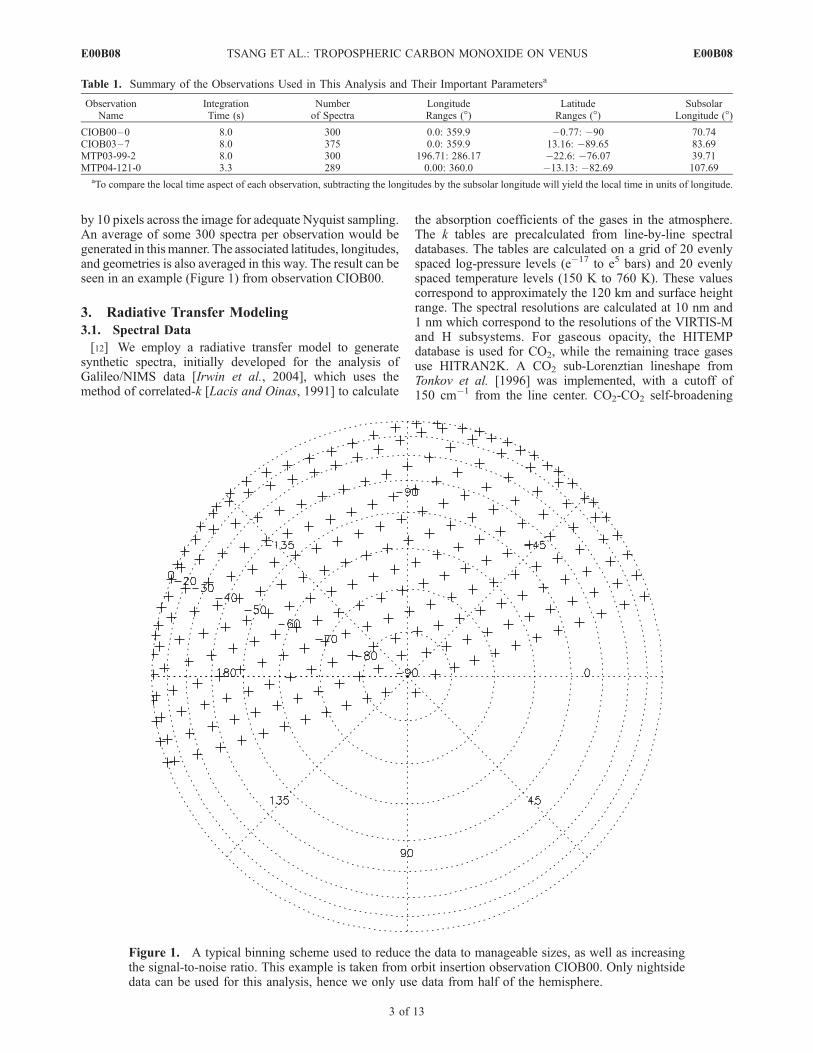
by 10 pixels across the image for adequate Nyquist sampling.An average of some 300 spectra per observation would begenerated in thismanner. The associated latitudes, longitudes,and geometries is also averaged in this way. The result can beseen in an example (Figure 1) from observation CIOB00.

3. Radiative Transfer Modeling

3.1. Spectral Data

[12] We employ a radiative transfer model to generatesynthetic spectra, initially developed for the analysis ofGalileo/NIMS data [Irwin et al., 2004], which uses themethod of correlated-k [Lacis and Oinas, 1991] to calculate

the absorption coefficients of the gases in the atmosphere.The k tables are precalculated from line-by-line spectraldatabases. The tables are calculated on a grid of 20 evenlyspaced log-pressure levels (e�17 to e5 bars) and 20 evenlyspaced temperature levels (150 K to 760 K). These valuescorrespond to approximately the 120 km and surface heightrange. The spectral resolutions are calculated at 10 nm and1 nm which correspond to the resolutions of the VIRTIS-Mand H subsystems. For gaseous opacity, the HITEMPdatabase is used for CO2, while the remaining trace gasesuse HITRAN2K. A CO2 sub-Lorenztian lineshape fromTonkov et al. [1996] was implemented, with a cutoff of150 cm�1 from the line center. CO2-CO2 self-broadening

Table 1. Summary of the Observations Used in This Analysis and Their Important Parametersa

ObservationName

IntegrationTime (s)

Numberof Spectra

LongitudeRanges (�)

LatitudeRanges (�)

SubsolarLongitude (�)

CIOB00–0 8.0 300 0.0: 359.9 �0.77: �90 70.74CIOB03–7 8.0 375 0.0: 359.9 13.16: �89.65 83.69MTP03-99-2 8.0 300 196.71: 286.17 �22.6: �76.07 39.71MTP04-121-0 3.3 289 0.00: 360.0 �13.13: �82.69 107.69

aTo compare the local time aspect of each observation, subtracting the longitudes by the subsolar longitude will yield the local time in units of longitude.

Figure 1. A typical binning scheme used to reduce the data to manageable sizes, as well as increasingthe signal-to-noise ratio. This example is taken from orbit insertion observation CIOB00. Only nightsidedata can be used for this analysis, hence we only use data from half of the hemisphere.


3 of 13

E00B08

half-widths were taken from the HITEMP database, whilethe CO2-H2O foreign half-widths were taken from Delaye etal. [1989]. The other remaining gases use the air-broadenedhalf-widths given in HITRAN2K. CO2 collision induced

absorption is parameterized according to Bezard et al.[1990], with a value of 3.5 � 10�8 cm�1 amagat�2 usedas the opacity factor.

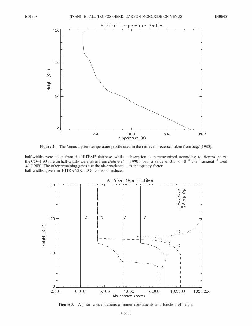
Figure 2. The Venus a priori temperature profile used in the retrieval processes taken from Seiff [1983].

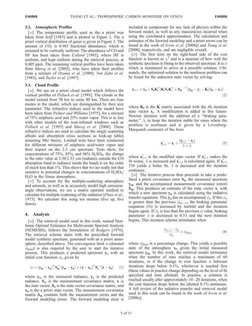
Figure 3. A priori concentrations of minor constituents as a function of height.


4 of 13

E00B08

3.2. Atmospheric Profiles

[13] The temperature profile used as the a priori wastaken from Seiff [1983] and is plotted in Figure 2. The apriori vertical distribution of gases is given in Figure 3. Theamount of CO2 is 0.965 fractional abundance, which isassumed to be vertically uniform. The abundance of CO andHF has been taken from Collard [1993], where HF isuniform, and kept uniform during the retrieval process, at0.005 ppm. The remaining vertical profiles have been takenfrom Marcq et al. [2005], who have taken their profilesfrom a mixture of Oyama et al. [1980], Von Zahn et al.[1983], and Taylor et al. [1997].

3.3. Cloud Profile

[14] We use an a priori cloud model which follows thevertical profiles of Pollack et al. [1993]. The clouds in themodel extend from 50 km to some 80 km. There are fourmodes in the model, which are distinguished by their sizeparameter. The refractive indices used in the model havebeen taken from Palmer and Williams [1975], for a mixtureof 75% sulphuric acid and 25% water vapor. This is in linewith other models of the near-infrared windows such asPollack et al. [1993] and Marcq et al. [2006]. Theserefractive indices are used to calculate the single scatteringalbedo and absorption cross sections as look-up tablesassuming Mie theory. Limited tests have been conductedfor different mixtures of sulphuric acid/water vapor andtheir impact on the 2.3 mm spectrum. Tests show, forconcentrations of 75%, 85%, and 96% H2SO4, the changeto the ratio value at 2.30/2.33 mm (radiance outside the COabsorption band to radiance inside the band) is on the orderof much less than 1%. This shows that we are really not thatsensitive to potential changes in concentrations of H2SO4/H2O in the Venus atmosphere.[15] To account for the multiple-scattering atmosphere

and aerosols, as well as to accurately model high emission-angle observations, we use a matrix operator method tocalculate for multiple scattering of the radiation [Plass et al.,1973]. We calculate this using ten streams (five up, fivedown).

4. Analysis

[16] The retrieval model used in this work, named Non-linear Optimal Estimator for Multivariate Spectral Analysis(NEMESIS), follows the formulation of Rodgers [1976].The retrieval scheme starts with the prescribed forwardmodel synthetic spectrum, generated with an a priori atmo-sphere, described above. The convergence limit f (denotedflimit) is also required by the user to start the iterativeprocess. This produces a predicted spectrum yn with aninitial cost function fi, given by

f ¼ ym � ynð ÞT S�1m ym � ynð Þ þ x� xað ÞT S�1

x x� xað Þ ð1Þ

where ym is the measured radiance, yn is the predictedradiance, Sm is the measurement covariance matrix, x isthe state vector, Sx is the state vector covariance matrix, andxa is the a priori state vector. The measurement covariancematrix Sm contains both the measurement errors and theforward modeling errors. The forward modeling error is

included to compensate for any lack of physics within theforward model, as well as any inaccuracies incurred whenusing the correlated-k approximation. The calculation andestimates of the forward modeling and a priori errors can befound in the work of Irwin et al. [2008a] and Tsang et al.[2008], respectively, and are negligible overall.[17] The first term on the right-hand side of the cost

function is known as c2 and is a measure of how well thesynthetic spectrum is fitting to the observed spectrum. It is fwhich is minimized to arrive at a possible solution. Ulti-mately, the optimized solution to the nonlinear problem canbe found for the unknown state vector by solving

xiþ1 ¼ xa þ SxKTi KiSxK

Ti þ Sm

� ��1ym � yi �Ki xa � xið Þð Þ

ð2Þ

where Ki is the K matrix associated with the ith iterationstate vector xi. A modification is added to this Gauss-Newton iteration with the addition of a ‘‘braking para-meter,’’ l, to keep the iteration stable for cases where theproblem is nonlinear and is given by a Levenberg-Marquardt constraint of the form

x0iþ1 ¼ xi þxiþ1 � xið Þ1þ l

ð3Þ

where x0i+1 is the modified state vector. If x0i+1 makes thefit worse, l is increased and x0i+1 is calculated again. If x0i+1239 yields a better fit, l is decreased and the iterationcontinues.[18] The iterative process then proceeds to take a prede-

fined a priori covariance error Sa, the measured spectrumym, and the accompanied measurement covariance (error)Sm. This produces an estimate of the state vector x, withwhich a new spectrum yn is calculated using the radiativetransfer equations. This yn has an accompanied fn. If this fn

is greater than the previous f(n�1), the braking parameter(equation (3)) is increased by tenfold and the iterationbegins again. If fn is less than the previous f value, brakingparameter l is decreased to 0.3l and the next iterationbegins. This iteration scheme terminates when

fn�1 � fn

fn

< flim it ð4Þ

where flimit is a percentage change. This yields a possiblestate of the atmosphere xi, given the initial measuredspectrum ym. In this work, the retrieval model terminateswhen the number of runs reaches a maximum of 60iterations, or if the change in cost function f betweeniterations drops below 0.1%, whichever is reached first(these values in practice change depending on the level of fitspecified and time allotted). In practice, a solution isreached usually after approximately 10–20 iterations, whenthe cost function drops below the allotted 0.1% minimum.A full review of the radiative transfer and retrieval modelused in this work can be found in the work of Irwin et al.[2008a].


5 of 13

E00B08

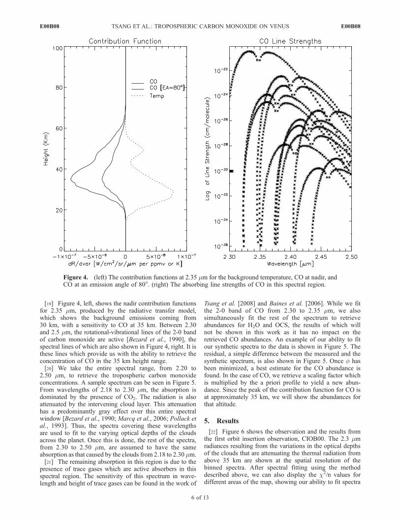
[19] Figure 4, left, shows the nadir contribution functionsfor 2.35 mm, produced by the radiative transfer model,which shows the background emissions coming from30 km, with a sensitivity to CO at 35 km. Between 2.30and 2.5 mm, the rotational-vibrational lines of the 2-0 bandof carbon monoxide are active [Bezard et al., 1990], thespectral lines of which are also shown in Figure 4, right. It isthese lines which provide us with the ability to retrieve theconcentration of CO in the 35 km height range.[20] We take the entire spectral range, from 2.20 to

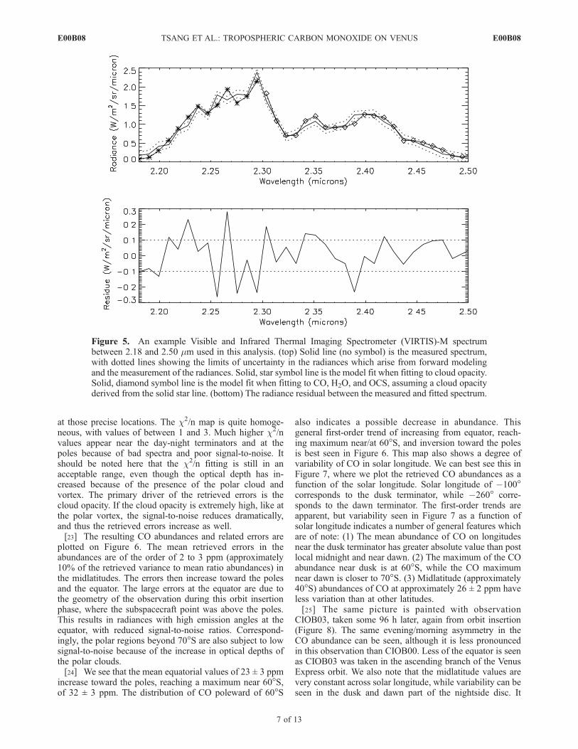
2.50 mm, to retrieve the tropospheric carbon monoxideconcentrations. A sample spectrum can be seen in Figure 5.From wavelengths of 2.18 to 2.30 mm, the absorption isdominated by the presence of CO2. The radiation is alsoattenuated by the intervening cloud layer. This attenuationhas a predominantly gray effect over this entire spectralwindow [Bezard et al., 1990; Marcq et al., 2006; Pollack etal., 1993]. Thus, the spectra covering these wavelengthsare used to fit to the varying optical depths of the cloudsacross the planet. Once this is done, the rest of the spectra,from 2.30 to 2.50 mm, are assumed to have the sameabsorption as that caused by the clouds from 2.18 to 2.30 mm.[21] The remaining absorption in this region is due to the

presence of trace gases which are active absorbers in thisspectral region. The sensitivity of this spectrum in wave-length and height of trace gases can be found in the work of

Tsang et al. [2008] and Baines et al. [2006]. While we fitthe 2-0 band of CO from 2.30 to 2.35 mm, we alsosimultaneously fit the rest of the spectrum to retrieveabundances for H2O and OCS, the results of which willnot be shown in this work as it has no impact on theretrieved CO abundances. An example of our ability to fitour synthetic spectra to the data is shown in Figure 5. Theresidual, a simple difference between the measured and thesynthetic spectrum, is also shown in Figure 5. Once f hasbeen minimized, a best estimate for the CO abundance isfound. In the case of CO, we retrieve a scaling factor whichis multiplied by the a priori profile to yield a new abun-dance. Since the peak of the contribution function for CO isat approximately 35 km, we will show the abundances forthat altitude.

5. Results

[22] Figure 6 shows the observation and the results fromthe first orbit insertion observation, CIOB00. The 2.3 mmradiances resulting from the variations in the optical depthsof the clouds that are attenuating the thermal radiation fromabove 35 km are shown at the spatial resolution of thebinned spectra. After spectral fitting using the methoddescribed above, we can also display the c2/n values fordifferent areas of the map, showing our ability to fit spectra

Figure 4. (left) The contribution functions at 2.35 mm for the background temperature, CO at nadir, andCO at an emission angle of 80�. (right) The absorbing line strengths of CO in this spectral region.


6 of 13

E00B08

at those precise locations. The c2/n map is quite homoge-neous, with values of between 1 and 3. Much higher c2/nvalues appear near the day-night terminators and at thepoles because of bad spectra and poor signal-to-noise. Itshould be noted here that the c2/n fitting is still in anacceptable range, even though the optical depth has in-creased because of the presence of the polar cloud andvortex. The primary driver of the retrieved errors is thecloud opacity. If the cloud opacity is extremely high, like atthe polar vortex, the signal-to-noise reduces dramatically,and thus the retrieved errors increase as well.[23] The resulting CO abundances and related errors are

plotted on Figure 6. The mean retrieved errors in theabundances are of the order of 2 to 3 ppm (approximately10% of the retrieved variance to mean ratio abundances) inthe midlatitudes. The errors then increase toward the polesand the equator. The large errors at the equator are due tothe geometry of the observation during this orbit insertionphase, where the subspacecraft point was above the poles.This results in radiances with high emission angles at theequator, with reduced signal-to-noise ratios. Correspond-ingly, the polar regions beyond 70�S are also subject to lowsignal-to-noise because of the increase in optical depths ofthe polar clouds.[24] We see that the mean equatorial values of 23 ± 3 ppm

increase toward the poles, reaching a maximum near 60�S,of 32 ± 3 ppm. The distribution of CO poleward of 60�S

also indicates a possible decrease in abundance. Thisgeneral first-order trend of increasing from equator, reach-ing maximum near/at 60�S, and inversion toward the polesis best seen in Figure 6. This map also shows a degree ofvariability of CO in solar longitude. We can best see this inFigure 7, where we plot the retrieved CO abundances as afunction of the solar longitude. Solar longitude of �100�corresponds to the dusk terminator, while �260� corre-sponds to the dawn terminator. The first-order trends areapparent, but variability seen in Figure 7 as a function ofsolar longitude indicates a number of general features whichare of note: (1) The mean abundance of CO on longitudesnear the dusk terminator has greater absolute value than postlocal midnight and near dawn. (2) The maximum of the COabundance near dusk is at 60�S, while the CO maximumnear dawn is closer to 70�S. (3) Midlatitude (approximately40�S) abundances of CO at approximately 26 ± 2 ppm haveless variation than at other latitudes.[25] The same picture is painted with observation

CIOB03, taken some 96 h later, again from orbit insertion(Figure 8). The same evening/morning asymmetry in theCO abundance can be seen, although it is less pronouncedin this observation than CIOB00. Less of the equator is seenas CIOB03 was taken in the ascending branch of the VenusExpress orbit. We also note that the midlatitude values arevery constant across solar longitude, while variability can beseen in the dusk and dawn part of the nightside disc. It

Figure 5. An example Visible and Infrared Thermal Imaging Spectrometer (VIRTIS)-M spectrumbetween 2.18 and 2.50 mm used in this analysis. (top) Solid line (no symbol) is the measured spectrum,with dotted lines showing the limits of uncertainty in the radiances which arise from forward modelingand the measurement of the radiances. Solid, star symbol line is the model fit when fitting to cloud opacity.Solid, diamond symbol line is the model fit when fitting to CO, H2O, and OCS, assuming a cloud opacityderived from the solid star line. (bottom) The radiance residual between the measured and fitted spectrum.


7 of 13

E00B08

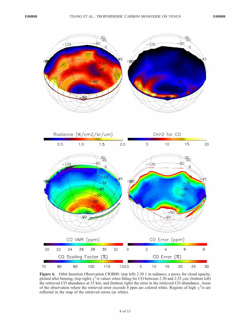
Figure 6. Orbit Insertion Observation CIOB00: (top left) 2.30 1 m radiance, a proxy for cloud opacity,plotted after binning; (top right) c2/n values when fitting for CO between 2.30 and 2.35 mm; (bottom left)the retrieved CO abundance at 35 km; and (bottom right) the error in the retrieved CO abundance. Areasof the observation where the retrieved error exceeds 8 ppm are colored white. Regions of high c2/n arereflected in the map of the retrieved errors (in white).


8 of 13

E00B08

should also be noted that the mean abundances at 60�S forCIOB00 and CIOB03 are 32 and 34 ± 2 ppm, respectively.[26] To investigate some of these features further, to

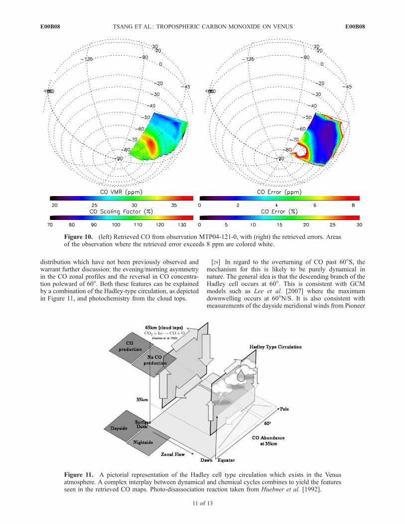
enhance the sampling and to see the if the degree ofvariability of CO concentrations changes over time, we takeobservations from the nominal orbit during ‘‘case 2’’ obser-vations, MTP03-99-2 andMTP04-121-0. These are shown inFigures 9 and 10, respectively. MTP03-99-2 shows a con-stant band of maximum CO abundance of between 35 to 36 ±2 ppm at a latitude of 60�S. Zonal variability at this latitudecan just be made out, with local maxima of CO at �90 and�135�W and a minimum at approximately �112�W, with avalue of 34 ppm. However, it should be noted that theretrieved error is of the order of these fluctuations andtherefore is not entirely without doubt. In addition, themaximum in CO commencing at 60�S continues at a steadyvalue until as high as 70�, where a slight decrease in theabundance past 70�S can be made out. The retrieved errorsin this region have not increased significantly. ObservationMTP04-121-0 shows a similar trend. Again, the CO max-imum is located at 60�S, with mean upper limit of 36 ±3 ppm, but in this instance seems more localized around alongitude of �45�W, decreasing by 3 ppm toward �68�W.However, caution should be taken again as this decrease is

of the order of the retrieved error. The decrease from 65�S inthe CO abundance to 30 ppm toward the poles is matchedby increased error caused by the increase in the cloudoptical depth of the polar vortex, decreasing the signal-to-noise ratio. Therefore, we cannot fully confirm the validityof the overturning from this image alone.

6. Discussion

[27] We first confirm the equator-to-pole increase of COin the troposphere first seen by Collard et al. [1993] fromGalileo/NIMS data, validated by Marcq et al. [2006] fromIRTF/SpeX data. It is also consistent with observationsmade by Marcq et al. [2008], using much higher spectralresolution subsystem of VIRTIS-H, who have shown verysimilar results for both equatorial and polar values of CO.The authors of the above work found a 30 ± 15% in- creasefrom 0� to 60�, corresponding to 24 ± 3 to 31 ± 2 ppm at36 km. This is very consistent with the results of this paper,which show on first order, an increase in the same latituderange of 23 ± 2 to 32 ± 2 ppm at the same altitude.[28] In addition, because of the unique imaging capabil-

ities of the VIRTIS-M subsystem, this analysis has alsopossibly revealed two new features in the tropospheric CO

Figure 7. The retrieved CO gradient versus latitude from CIOB00 observation, plotted as a function ofsolar longitude, interpolated in spacings of 5�. These retrieved CO abundances are referenced to 35 km.Dusk terminator at �100� and dawn terminator at �260�.


9 of 13

E00B08

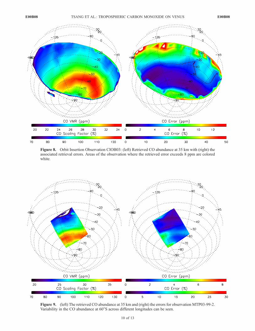
Figure 9. (left) The retrieved CO abundance at 35 km and (right) the errors for observation MTP03-99-2.Variability in the CO abundance at 60�S across different longitudes can be seen.

Figure 8. Orbit Insertion Observation CIOB03: (left) Retrieved CO abundance at 35 km with (right) theassociated retrieval errors. Areas of the observation where the retrieved error exceeds 8 ppm are coloredwhite.


10 of 13

E00B08

distribution which have not been previously observed andwarrant further discussion: the evening/morning asymmetryin the CO zonal profiles and the reversal in CO concentra-tion poleward of 60�. Both these features can be explainedby a combination of the Hadley-type circulation, as depictedin Figure 11, and photochemistry from the cloud tops.

[29] In regard to the overturning of CO past 60�S, themechanism for this is likely to be purely dynamical innature. The general idea is that the descending branch of theHadley cell occurs at 60�. This is consistent with GCMmodels such as Lee et al. [2007] where the maximumdownwelling occurs at 60�N/S. It is also consistent withmeasurements of the dayside meridional winds from Pioneer

Figure 10. (left) Retrieved CO from observation MTP04-121-0, with (right) the retrieved errors. Areasof the observation where the retrieved error exceeds 8 ppm are colored white.

Figure 11. A pictorial representation of the Hadley cell type circulation which exists in the Venusatmosphere. A complex interplay between dynamical and chemical cycles combines to yield the featuresseen in the retrieved CO maps. Photo-disassociation reaction taken from Huebner et al. [1992].


11 of 13

E00B08

Venus which indicate the horizontal convergence of themeridional flow is greatest between 50 and 60� [Limaye,2007]. We expect the maximum downwelling of the Hadleycell to be associated with regions of maximum verticalwinds, and therefore would bring the most CO rich air frommesosphere (>65 km) to the troposphere. If this downwel-ling is greatest at 60�, it implies a poleward decrease in COconcentration past 60�S, and therefore would be consistentwith our observations.[30] The situation with respect to the east-west asymme-

try in the CO abundances is probably a mixture of photo-chemistry and dynamics processes, which is responsible forthe concentration of CO at this altitude since the dominantchemistry occurs way above or way below this 35 kmregion. The supply of CO is governed by the upperatmosphere source. The two options to create this east-westasymmetry in CO at 35 km is either an east-west gradient inthe source of CO in the source region and constant downw-elling, or a constant source of CO in the source region andan east-west gradient in the downwelling across longitudes.It is indeed likely to be a combination of both processes.[31] The evening/morning asymmetry seen in Figures 6

and 8 can be, on first order, simply a function of thephotochemistry which is occurring at the cloud tops at65 km. If we consider what is occurring at the cloud tops,during the early morning, we would expect a minimum inthe early morning with a ramp up of CO production in themorning sunshine due to the photolysis by solar UV, andwould depend on the photolysis rate of CO above theclouds. This would peak in the early evening (before sunsetprobably). Maps of CO on the nightside of Venus above theclouds [Irwin et al., 2008b] indicate enhanced CO at theevening terminator and are consistent with these observa-tions of the tropospheric CO and photochemical mecha-nisms above the clouds. As the photolysis stops because ofthe lack of sunlight, no more CO is produced on thenightside. The meridional circulation, however, will continueto pump mesospheric air into the lower troposphere. At thestart of the evening you would therefore expect highabundances of CO in the lower atmosphere at the locationof the downwelling of the Hadley cell and for this concen-tration to decay as the night progresses, assuming thevertical velocity of this downwelling was constant acrossthe nightside (which is most likely not the case). However,CO is constantly being destroyed by sink reactions, mostnotably by OCS [Pollack et al., 1993] and S2 [Hong andFegley, 1997], and reconverted back to CO2. Therefore, wealso need to know something about the creation anddestruction rates for CO in the lower atmosphere, as wellas the meridional overturning rates (10 m s�1 polewardwinds at 100 mbar). From the observations of Figures 6and 8, a change in the concentration of CO of 2 ppm fromthe evening to morning terminator can be seen. There maybe some problem accounting for this given what is knownabout the reaction rates and atmospheric dynamics.

7. Conclusions

[32] Observations of the nightside of Venus taken fromVenus Express/VIRTIS-M instrument at wavelengths be-tween 2.20 to 2.50 mm have been used to measure and mapthe distribution of CO in the troposphere of Venus. We have

taken spectra from four different observations, two fromorbit insertion, and two from the nominal orbit, which arethen coadded and binned for increased signal-to-noise andhomogeneous spatial sampling. We use a spectral fittingalgorithm to first account for variations in the cloud opticaldepth by fitting spectra from 2.20 to 2.30 mm. This isthen followed by fitting the remaining spectra from 2.30 to2.35 mm, which is sensitive to the 2-0 CO band, by scaling aknown a priori profile.[33] We first confirm the presence of the CO enhance-

ment from equator to pole, with a mean increase of between40% and 45% from 23 ± 2 ppm to 32 ± 2 ppm, which isconsistent with observations made by the Galileo/NIMSflyby of Venus in 1990. We find the peak value of CO tooccur between 55 and 65�S. We also find evidence of twopossibly new features in this CO gradient; decreases of COpoleward of 60�S and variability in longitude.[34] A mixture of photochemistry and dynamics will be

responsible for the concentration of CO at this altitudebecause the dominant chemistry does not occur near 35 km.Advection of CO from below is unlikely because of a lack ofa continuous source, leaving photolysis of CO2 above 60 kmas the most likely source of CO in the lower atmosphere.The CO is then advected into the lower atmosphere,particularly in the downwelling region near 60�, where itis destroyed. Given the need for sunlight to photolyse theCO2, the distribution of CO at the source altitude probablyfollows the solar zenith angle, peaking in the afternoonhemisphere because of the background flow. Polewardadvection in the source region and downwelling at the polesthen transports the CO into the lower atmosphere, produc-ing the observed latitudinal gradient at 35 km. Theseobservations would then place the downwelling branch ofthe Hadley cell near 60�, consistent with observations ofpeak westward flow at 60� and GCM simulations such asLee et al. [2007]. It is also consistent with measurements ofthe dayside meridional winds from Pioneer Venus whichindicate the horizontal divergence (converging air mass) ofthe meridional flow is greatest between 50 and 60� [Limaye,2007]. Poleward of 60�, the vortex ‘‘barrier’’ and decreasingsunlight would contribute to a negative latitudinal gradientin CO, as observed. In addition, the fact that we observe theCO gradient at 35 km, which is a proxy for the returnbranch of the Hadley cell, implies the vertical extent of thecell(s) is at least 40 km.

[35] Acknowledgments. I would like to thank Emmanuel Marcq forhis discussions of CO and his work with VIRTIS-H spectra and its findings.We would also like to thank Frank Mills and Robert Carlson for theirdiscussions on this subject. This work was made possible from fundinggiven by the United Kingdom Science Technology Facilities Council, aswell as the continued support of CNES and ASI.

ReferencesAllen, D., and J. Crawford (1984), Cloud structure on the dark side ofVenus, Nature, 307, 222–224, doi:10.1038/307222a0.

Baines, K., S. Sushil Atreya, R. Carlson, D. Crisp, P. Drossart, V. Formisano,S. Limaye, W. Markiewicz, and G. Piccioni (2006), To the depths ofVenus: Exploring the deep atmosphere and surface of our sister worldwith Venus Express, Planet. Space Sci., 54, 1263–1278, doi:10.1016/j.pss.2006.04.034.

Bezard, B., C. de Bergh, D. Crisp, and J. Maillard (1990), The deep atmo-sphere of Venus revealed by high-resolution nightside spectra, Nature,345, 508–511, doi:10.1038/345508a0.

Carlson, R., K. Baines, T. Encrenaz, F. Taylor, P. Drossart, L. Kamp,J. Pollack, E. Lellouch, and A. Collard (1991), Galileo infrared imaging


12 of 13

E00B08

spectroscopy measurements at Venus, Science, 253, 1541 – 1548,doi:10.1126/science.253.5027.1541.

Collard, A. (1993), Thermal emission from the nightside of Venus, D.Phil.thesis, Univ. of Oxford, UK.

Collard, A., F. Taylor, S. Calcutt, R. Carlson, L. Kamp, and K. Baines(1993), Latitudinal distribution of carbon monoxide in the deep atmo-sphere of Venus, Planet. Space Sci., 41(7), 487–494.

Coradini, A., et al. (1998), VIRTIS: An imaging spectrometer for theRosetta mission, Planet. Space Sci., 46(9–10), 1291–1304.

Counselman, C., S. Gourevitch, R. King, G. Loriot, and E. Ginsberg(1980), Zonal and meridional circulation of the lower atmosphere ofVenus determined by radio interferometry, J. Geophys. Res., 85, 8026–8030, doi:10.1029/JA085iA13p08026.

Delaye, C., J. Hartmann, and J. Taine (1989), Calculated tabulations of H2Oline broadening by H2O, N2, O2, and CO2 at high temperature, Appl.Opt., 28(23), 5080–5087.

Drossart, P., et al. (2007), Scientific goals for the observation of Venus byVIRTIS on ESA/Venus Express mission, Planet. Space Sci., 55, 1653–1672, doi:10.1016/j.pss.2007.01.003.

Fegley, B. J., M. Y. Zolotov, and K. Lodders (1997), The oxidation state ofthe lower atmosphere and surface of Venus, Planet. Space Sci., 125,416–439.

Gierasch, P. (1975), Meridional circulation and the maintenance of theVenus atmospheric rotation, J. Atmos. Sci., 32, 1038–1044, doi:10.1175/1520-0469(1975)032<1038:MCATMO>2.0.CO;2.

Hong, Y., and B. Fegley (1997), Formation of carbonyl sulphide (OCS)from carbon monoxide and sulphur vapour and applications to Venus,Icarus, 130, 495–504, doi:10.1006/icar.1997.5824.

Huebner, W. F., J. J. Keady, and S. P. Lyon (1992), Solar photon rates forplanetary atmospheres and atmospheric pollutants, Astrophys. Space Sci.,195, 1–294, doi:10.1007/BF00644558.

Irwin, P., P. Parrish, T. Fouchet, S. Calcutt, F. Taylor, A. Simon-Miller, andA. Nixon (2004), Retrievals of Jovian tropospheric phosphine fromCassini/CIRS, Icarus, 172, 37–49, doi:10.1016/j.icarus.2003.09.027.

Irwin, P. G. J., N. Teanby, R. de Kok, L. Fletcher, C. Howett, C. C. C.Tsang, C. F. Wilson, S. B. Calcutt, C. Nixon, and P. Parrish (2008a), TheNEMESIS planetary atmosphere radiative transfer and retrieval tool,J. Quant. Spectrosc. Radiat. Transf., 109, 1136–1150, doi:10.1016/j.jqsrt.2007.11.006.

Irwin, P. G. J., R. de Kok, A. Negrao, C. C. C. Tsang, C. F. Wilson,P. Drossart, G. Piccioni, D. Grassi, and F. W. Taylor (2008b), Spatialvariability of carbon monoxide in Venus’ mesosphere from VenusExpress/VIRTIS Visible and Infrared Thermal Imaging Spectrometermeasurements, J. Geophys. Res., 113, E00B01, doi:10.1029/2008JE003093.

Kamp, L., F. Taylor, and S. Calcutt (1988), Structure of Venus’s atmospherefrom modelling of night-side infrared spectra, Nature, 336, 360–362,doi:10.1038/336360a0.

Karaiskou, A. C., C. Vallance, V. Papadakis, I. M. Vardavas, and T. P.Rakitzis (2004), Absolute absorption cross-section measurements ofCO2 in the ultraviolet from 200 to 206 nm at 295 and 373 K, Chem.Phys. Lett., 400, 30–34.

Krasnopolsky, V. A. (2007), Chemical kinetic model for the lower atmo-sphere of Venus, Icarus, 191, 25–37, doi:10.1016/j.icarus.2007.04.028.

Lacis, A., and V. Oinas (1991), A description of the correlated k-distribu-tion method for modeling non-grey gaseous absorption, thermal emissionand multiple scattering in vertically inhomogeneous atmospheres, J. Geo-phys. Res., 96, 9027–9063, doi:10.1029/90JD01945.

Lee, C., S. Lewis, and P. Read (2007), Superrotation in a Venus generalcirculation model, J. Geophys. Res., 112, E04S11, doi:10.1029/2006JE002874.

Limaye, S. (2007), Venus atmospheric circulation: Known and unknown,J. Geophys. Res., 112, E04S09, doi:10.1029/2006JE002814.

Marcq, E., B. Bezard, T. Encrenaz, and M. Birlan (2005), Latitudinal var-iations of CO and OCS in the lower atmosphere of Venus from near-infrared nightside spectro-imaging, Icarus, 179, 375–386, doi:10.1016/j.icarus.2005.06.018.

Marcq, E., T. Encrenaz, B. Bezard, and M. Birlan (2006), Remote sensingof Venus’ lower atmosphere from ground-based spectroscopy: Latitudinaland vertical distribution of minor species, Planet. Space Sci., 54, 1360–1370, doi:10.1016/j.pss.2006.04.024.

Marcq, E., B. Bezard, P. Drossart, and G. Piccioni (2008), A latitudinalsurvey of CO, OCS, H2O and SO2 in the lower atmosphere of Venus:Spectroscopic studies using VIRTIS-H, J. Geophys. Res., doi:10.1029/2008JE003074, in press.

Oyama, V., G. Carle, F. Woeller, J. Pollack, R. Reynolds, and R. Craig(1980), Pioneer Venus gas chromatography of the lower atmosphere ofVenus, J. Geophys. Res., 85, 7891–7902, doi:10.1029/JA085iA13p07891.

Palmer, K., and D. Williams (1975), Optical constants of sulfuric acid;Application to the clouds of Venus?, Appl. Opt., 14(1), 208–219.

Piccioni, G., et al. (2007), VIRTIS: The Visible and Infrared ThermalImaging Spectrometer, ESA Spec. Publ. SP-1295, pp. 1–27, Eur. SpaceAgency, Paris.

Plass, G. N., G. W. Kattawar, and F. E. Catchings (1973), Matrix operatortheory of radiative transfer: 1. Rayleigh scattering, Appl. Opt., 12, 314–329.

Pollack, J., J. Dalton,D.Grinspoon,R.Wattson, R. Freedman,D. Crisp,D.Allen,B. Bezard, C. de Bergh, and L. Giver (1993), Near-infrared light fromVenus’ nightside: A spectroscopic analysis, Icarus, 103, 1 – 42,doi:10.1006/icar.1993.1055.

Rodgers, C. (1976), Retrieval of atmospheric temperature and compositionfrom remote measurements of thermal radiation, Rev. Geophys., 14(4),609–624, doi:10.1029/RG014i004p00609.

Seiff, A. (1983), Thermal structure of the atmosphere of Venus, in Venus,pp. 215–279, Univ. of Ariz., Tucson.

Shemansky, D. E. (1972), CO2 extinction coefficient 1700–3000 A,J. Chem. Phys., 56, 1582–1587, doi:10.1063/1.1677408.

Taylor, F. (1995), Carbon monoxide in the deep atmosphere of Venus, Adv.Space Res., 16(6), 81–88, doi:10.1016/0273-1177(95)00253-B.

Taylor, F., D. Crisp, and B. Bezard (1997), Near-infrared sounding of thelower atmosphere of Venus, in Venus II: Geology, Geophysics, Atmo-sphere, and Solar Wind Environment, pp. 325–351, Univ. of Ariz. Press,Tucson.

Tonkov, M., N. Filippov, V. Bertsev, J. Bouanich, V.-T. Nguyen, C. Brod-beck, J. Hartmann, C. Boulet, and F. Thibault (1996), Measurements andempirical modeling of pure CO2 absorption in the 2.3 mm region at roomtemperature: Far wings, allowed and collision- induced bands, Appl. Opt.,35(24), 4863–4870.

Tsang, C. C. C., P. G. J. Irwin, F. W. Taylor, and C. F. Wilson (2008), Acorrelated-k model of radiative transfer in the near infrared windows ofVenus, J. Quant. Spectrosc. Radiat. Transf., 109, 1118–1135, doi:10.1016/j.jqsrt.2007.12.008.

Von Zahn, U., S. Kumar, H. Niemann, and R. Prinn (1983), Composition ofthe Venus atmosphere, in Venus, pp. 299–430, Univ. of Ariz., Tucson.

��B. Bezard and P. Drossart, LESIA, Observatoire de Paris, 5 place Jules

Janssen, F-92195 Meudon, France.S. Calcutt, R. de Kok, P. G. J. Irwin, F. W. Taylor, C. C. C. Tsang, and

C. F. Wilson, Atmospheric, Oceanic and Planetary Physics, ClarendonLaboratory, Department of Physics, University of Oxford, Parks Road,Oxford OX1 3BH, UK. ([email protected])C. Lee, Geophysics and Planetary Sciences, California Institute of

Technology, MC 150-21, Pasadena, CA 91125, USA.G. Piccioni, INAF-IASF, Via del Fosso del Cavaliere 100, I-00133 Rome,

Italy.


13 of 13

E00B08

tropospheric carbon monoxide concentrations and...

Documents