Effects of the 2006 El Niiio on tropospheric ozone and carbon

monoxide: Implications for dynamics and biomass burning

S. Chandra1>" J. R. ~iemke"'", E3. N. Duncan"" and T. L. Diehll*"

' ~odda rd Earth Sciences and Technology Center, Universitp of Maryland Balti~nore County,

Baltimore, Maryland, USA

'NASA Goddard Space Flight Center, Greenbelt, Maryland, USA

We have studied the effects of the 2006 El Nifio on tropospheric 0 3 and GO at

tropical and sub-tropical latitudes measured from the OM1 and MLS instruments on the Aura

satellite. The 2006 El Niiio-induced h u g h t allowed forest fires set to clear land to burn out of

conh-ol during October and November in the Indonesian region. The effects of these fires are

clearly seen in the enhancement of GO concentration measured from the MLS instrument. We

have used a global model of atmospheric chemistry and h-ansport (GMI CTM) to quantify the

relative irrrportance of biomass burning and large scale transport: in producing observed changes

in tropospheric O3 and 6 0 . The model results show that during October and November both

biomass burning and meteorological changes cofllributed almost equally to the obsemed increase

in tropospheric Q3 in the Indonesian region. The biomass component was 4-6 DU but it was

limited to the Indonesian region where the fires were most intense, The dynamical component

was 4-8 DU but it covered a much larger area in the Indian Ocean extending from South East

Asia in the nordh to western Australia in the south. By December 2006, the effect of biomass

taming was reduced to zero and the obsemed changes in tropospheric O3 were mostly due to

dynamical effects. The model results show an increase of 2-3% in the global burden of

tropospheric ozone. In comparison, the global burdean of GO increased by 8-12%.

https://ntrs.nasa.gov/search.jsp?R=20080047927 2018-05-29T04:18:08+00:00Z

1 Introduction

El Niiio and La Niiia events are major sources of inter-annual and decadal variability in tropical

tropospheric ozone (a3) [e.g., Ziemke et al. 30031. The atmospheric effects of El Nifio events are

generally a change in convection in the tropical troposphere associated with an eastward shift of

the warm SST anomaly and large scale Walker circulation. This shift results in an increase in

tropospheric column O3 in the western Pacific and a decrease in the eastern Pacific relative to

non-El Niiio years. The effect of El Niiio on specific humidity is usually opposite to that of

column ozone [e.g., Chandrcz et al., 1998; 20071. During La Nifia years, dynamical processes are

largely reversed which results in a decrease (increase) of column ozone (specific humidity) in the

western Pacific, The effects of El Nifio on tropospheric composition have been extensively

studied from both satellite and ground based measurements [e.g., ChancIrc~ et al., 1998; Fujiwara

et al., 1999; T?~ompson et al., 20011 and by using global models of atmospheric chemistry and

transport [e.g., Peters et ul., 2001; Sudo and Takahushi, 2001; Chmdru et LII., 2002, 2003;

Dzlncun et al., 2003; Zeng cmd Pyle, 2005; Doherty et al., 20061

Recently Logun et al. [2008] studied the effects of the 2004 and 2006 El Niiio events on

tropospheric profiles of CO, 03, and Hz0 measured from the Tropospheric Emission

Spectrometer (TES) on the Aura satellite. Their findings were generally consistent with the

observed characteristics of O3 and H20 inferred from previous El Niiio events. The changes

during the 2004 El Nifio in tropospheric O3 and Hz0 fiom TES are similar to those inferred from

Ozone Monitoring Instrument (OMI) and Microwave Limb Spectrometer (MLS) flown on the

same satellite [Clgandru et ul., 20071. The 2004 El NiAo was a weak event compared to 2006

and significantly weaker compared to the El NiAo of 1997-1998. This was reflected in the TCO

(tropospheric column ozone) anomaly over the Indonesian region in the western Pacific as

shown in Table 1 of Logan et al. [2008]. For example, the TCO anomaly in November 1997

inferred from EP TOMS was 14.4 Dobson Units (DlJ; 1 DU = 2.69 x 10" molecules-m-*). The

corresponding values from TES for November 2004 and 2006 were 6.6 DU and 1 I . 1 DU. Logan

et ul. [2008] attributed most of these changes to differences in the magnitude of CO emissions

from fires in Indonesia which in these years were estimated to be 193 Tg, 24 Tg, and 82 Tg,

respectively. They also suggested significant contribution fiom NOx production due to lightning

in late No~ember and Ilecember 2006 \then CO prod~tction due to large scale forest fires

decreased significantly. The effects of forest fires in the Indonesian region during the 1997 El

NiAo was studied by Cfiundru ct GI. [2002] using the GEOS-C'HEM global model of chemistry

and transport. Their study suggested that about half of the increase in tropospheric colun~n

07one in the Indonesian region was due to biomass burning and the other half due to dy~lamical

effects. A similar conclusion was arrited by Sndo crnd 7ukclhtr.shi [2001j from their modcl study.

Their conclusion about the contribution of bio~nass burning was indirect since they did not

explicitly include the effect of biomass burning in their model study,

The combined OMI and MLS instruments on the Aura satellite hace been prokiding ncar global

rneasurernents of TCO from August 2004 to present [e.g., Zicmke et ul., 2006; Schocherl ct ul.,

20071 as discussed in Section 2. In addition the hlLS instn~rrlent has been providing daily

measurements of CO at seteral pressure letels in the troposphere and stratosphere [i,ive~cy ef ul.,

20081. The purpose of this paper is to study the effects of the 2006 El Nifio on tropospheric

composition measured f?om the OM1 and MLS instruments on the Aura satellite arid evaluate

specific roles of the karious processes using a global model of chemistry and transport. 'The

global model used in this study is the NASA GMI CTM (Global Modeling Initiative Chemical

Transport Model). It successfully simulates a wide range of observations of chemical

constituents in the troposphere and stratosphere, including data collected by instnltlients on

board satellites. We provide a brief overview of the relevant tropospheric processes in the GMI

CTM in section 3. In our study, the El NiAo related changes in O3 and CO fields based on OM1

and MLS measurements are compared with corresponding changes based on GMI C'TM

simulation to delineate the relative importance of biomass burning and large scale transport.

In the hllowing, section 2 discusses the satellite data, cection 3 the (;MI nod el, and sections 4

and ti compare obsertcd and lneasured 0 1 and CO, respectively. Section 6 discusscs the impact

of biomass burning emissions over Indonesia during the 2006 El Nifio, and section 7 compares

the strength and frcclucncy of the 2006 and recent El NiCo etents with pretious El Nirlo events.

Finally, section 8 proc ides a summary.

2 Measurements from OkIB and ML,S

OM1 is one out of a total of four instruments onboard the Aura spricecraft, which is llown in a

sun-synclironous polar orbit at 705 km altitude uith a 98.2'' inclination. 'rhe spacecraft has an

eclliatorial crossing time of 1 :45 pm (ascending node) with around 98.8 lnit~utes per orbit ( 14.6

orbits per day on average). Oh11 is a nadir-scanning instrument that for cisible (3.50-500 nm)

and UV \tavelength channels (IJV-l: 270-314 run; lJV-3,: 306-380 nm) detects backscattcrcd

solar radiance to measure column o;zonc with near global cokerage (aside from polar night

latitudes) over the Earth with a resolution of 13 km x 24 km at nadir. t3esides ozone OM1 also

tneasltres cloud-top pressure, aerosols and aerosol parameters, NOz, SOz, arid other trace

constituents in the troposphere aritf ctratosphere [L,evrlt et Id., 20061. 'Total ozone from OM1 is

de r i~ed from the TOMS version 8 i~lgorithm. A description of this algorithm may be obtained

from the 'TOMS V8 CU DVD ROM, or iiom the OM1 Algorithm Theoretical Basis Document

(A'TRD) (from the webpage http:/~torns.gsfc.nasa.gov/\ ersion8/~8torns_ittbd.pdf).

There are two standard OM1 total oione products. Here we use data from the collection 3

OMT03 version 8.5 (v8.5) product that is based on the 'Total Ozone Mapping Spectrometer

(TOMS) version 8 (v8) total O3 algorithm. A description o f this algorithm may be obtained from

the '['OMS t 8 DVD or the OhII Algorithm 'Theoretical Basis Document (ATBD) frorn the

TOMS u eb page kttp:,!ton1s.gsfc.n~~c;a.aov/tcrsion8it 8toms ntbd.udf. A main difference

bctvveen t 8 and v8.5 is that t8.5 uses measured cloud pressure whereas v8 and earlier versions

used an infrared-measured climatology for cloud pressure. Another OM1 algorithm based on the

Differential Optical Absorption Spectroscopy Method (ZIOAS) tcchniclue gives similar estimates

of total column omne [Kroon et ul., 2008bl. 'These total column O3 retrievals have been

compared with ground-based data [,McPc~tcrs et ~zl., 20081 and aircraft-based measurements

[ki-onn rt LIE. , 2 OOSa].

O3 protiles from the Aura blicrowate Limb Sounder (MLS) are used to estimate stratospheric

column O1 (SCO). 'The SCO is subtractcd from OM1 total column O 3 frorn OM1 to yield

tropospheric colulnn 0 3 and mcan volume mixing ratio [c.g., Zicwzkt. ct ~ d . , 20061. The mean

coli~~rie mixing ratio (units ppbv) is determined by taking tropospheric column O3 (in [lobson

I 'ritts, I) l i ) and ciitiding thiv by pressure difference (in irrlits hI%a) bctneen surtilcc and

tropop:zrrsr, and thcn nnrtltiplying this by the fitctor 1.27. Valid:ition of MISS \. 2 2 rneasurcrt~ents

is ctix.uc\t.cf by Fi.n;t/cvirz~x cPt LIE. [ZOO81 and i,it*t.scy c7f crl [IlOl)tl]. I he mcasilremcnts of rrierrn

troposphcric O3 from OMIIMLS and upper tropospheric CO from MLS are studied and

compared with simulations froin a global chemical transport rnodel (discussed next).

3 NASA Global Modeling Initiative Chemical 'Transport Model

The <;MI CTM is described and e.caluated in Ziemkc ct ul. [2006], Schoehcrl et 01. 120061,

Str~zhan et a/. [2007] and Dunc.un ct LEI. 12007, 20081. Thc chemical mechanism includes 117

species, 322 chemical reactions, and 81 photolysis reactions to simulate troposphcric and

stratospheric chemistry. It irlcludes a detailed description of 0;-NOx-hydrocarbon chemistry,

updated with rcccnt experimental data. The chenlical Inass balance eq~iations are integrated

using the SMVGEAK 11 algorithm [Jacobson, 19951. Photolysis frequencies are computed using

the Fast-JX radiative transkr algorithm (M. Prather, pcr.sonu1 comrntcrzicution). The algorithm

treats both Rayleigh scattering as kvell as Mie scattering by clouds and aerosol. The CTM

sitnulates the radiati~e and heterogeneous chemical effects of sulfate, dust, sea-salt, organic

carbon and black carbon aerosol on trctpospheric photochen~istry.

Biogenic emissions of isoprene and rnonoterpenes are calculated on-line as described in

Gtlenther et (21. [2006]. The lightning NOx parameterization fits the relationship between tnodel-

calculated convectike mass fluxes and obserced cloud-to-ground flash rates (D. Allen and K.

Pickering, pprsoncrl c.oi?li?2~micution). Tirne-appropriate anthropogcnic and biomass burning

emissions include, surface emissions from industryifossil fuel, biomass burning, biogenic and

biofuel combustions and contributions from aircraFt emissions. They are based on the Global Fire

Emission Database, version 2 (CiFEDv2) and discussed in the GMI CTM papers listcd above.

Monthly total biomass burning of CO and NOx are shown in Table 1 for the later part of 2006

when the Indonesian fires cvere most intense.

Table 1 indicates that the Indonesian fires increased the C'O burden by 69 Tg during the thrce

month period from September to November 2006. It is about 27% of the global CO burden (25 1

Tg) during the same period. The increase in NOx due to Indonesian fires during the Yame period

was 1.19 Tg compared to thc global burden of about 19.4 Tg.

The rneteorologicd fields that drive transport are from the (ioddatd hlc;ldeling and ,2ssimilation

Office (CiMAO) 4iEOS-4 data assimilation system ((;EOS-4-ILdAS) [EElc~om gf LII,, 30051.

Feattarcc of the circttlation, strch as anticyclones. in the (;MI C TM arc;: realistically t-izpresentcd in

the simulations because of the data constraints on rneteorological analyses. The CjEOS-4-IIAS

fields have been regrictded to 42 kertical Ic\icls uith a lid at 0.01 hPa. The horizontal resolution

is 2.5" x 2" (longitude by latitude).

14 validation of the global model tared in this study is; ghcn in the Appendix. Thic analysis

compares the ~ o n a l and seasonal variability of 'TC'O derived frorn the model uith obsened

variability fiom OMIIfMLS.

4 Model comparison of El Nifio related changes in O3 with satellite measurements

As in C'h~intlru tlt (21. [2007] and Logcm ct c r l . [2008], we hate cllosen October, Noventber and

Decembcr 2005 as a baseline for estimating El Nifio-related changes in these months in the

preceding and the following year. Year 2005 was a neutral year from an El Nifio perspectike.

Maps of tropospheric O3 mean mixing ratio are sho-\vn in Figure la for October 2004, 2005, and

2006. 'They show relative changes in oyone in the El NiAo years (upper and lower panels) with

respect to a non El NiAo year (middle panel). All three panels show regions of miriirnum values

near the dateline. Ifowever, both the upper and the lower panels show a greater eastward shift

across the dateline which results in an incrcase of about 6-1 5 ppbv ( 3- 10 IXJ) oter the western

Pacific region and a decrease of smaller magnitude east of the dateline. The increase in O3 mean

mixing ratio is larger in October 2006 (lower panel) which is colisistent with a relatively stronger

El Nifio etent in 2006 compared to 2004. The model (Figure lb) captures most of the zonal

characteristics of TCO shown in Figure la, but it tends to underestimate the obsened \ialues by

5- 10 ppbv over most of the region betwcen i I0 deg. (Figure lc). Outside this region the sign is

reversed and the model is biased higher by about the same magnitude. These pattern shifts in the

model and observation are comparable in November and December months (not shown) arld are

similar to those shown in Figure 2 of Ziernke et crl[2000] h r the 1997 El Nifio event.

The El Niiio related changes in ozone mean mixing ratio in 2006 are clearly discernible in

Figures La, 3b and 2c. 'Thew figures show differences in OhII,'ML,S O3 (top panels) arid the

~nodel 0; (bottom panels) between years 2006 and 2005 for the months of October-Ileccmber.

rhe model 3 r d obser~ed balucs are generally in good agreement except in the \testern F'acitic

region in Octobcr {Figure 22) where the model \ialucs are biased highcr. Ihis bias is also

rctlccteci in C'O as iilcficatcd i r i wction 5 tlnd ic probably d ~ i e to okerestirnation of the cftect of

biomass burning in the Indonesian region in October 2006. In general, obsemvations and model

indicate excellent agreement in characterizing both broad and small scale features including the

dipole nature of ozone anomaly in the tropical Pacific region (Figures 2a and 2c). The large

negative anomaly over eastern A&icdIndian Ocean in December 2006 seen in the data (Figure

2c) is a manifestation of dynamically induced changes and is well produced in the model. We

have analyzed the model results to estimate the contributions of the upper (above 500 hPa) and

the lower troposphere in producing the El Niiio related changes in tropospheric ozone. In

general, the contributions &om the upper and the lower troposphere are almost equal. However,

the large negative anomaly in December In the eastern Akicailndian Ocean (Figure 2c) comes

mostly h m the upper troposphere.

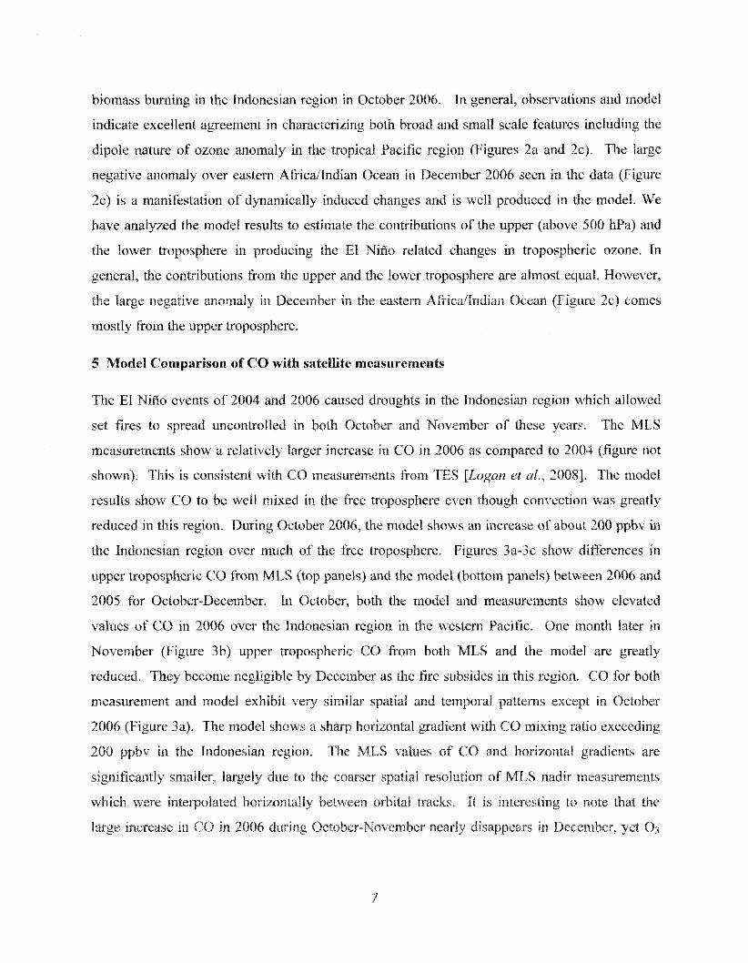
5 Model Comparison of CO with satellite measurements

The El Nilio events of 2004 and 2006 caused droughts in the Indonesian region which allowed

set fires to spread uncontrolled in both October and November of these years. The MLS

measurements show a relatively larger increase in CO in 2006 as compared to 2004 (figure not

shown). This is consistent with CO measurements from TES [Logun et ul., 20081. The model

results show CO to be well mixed in the free troposphere even though convection was greatly

reduced in this region. During October 2006, the model shows an increase of about 200 ppbv in

the Indonesian region over much of the free troposphere. Figures 3a-3c show differences in

upper t-ropospheric CO from MLS (top panels) and the model (bottom panels) between 2006 and

2005 for October-December. In October, both the model and measurements show elevated

values of C 0 in 2006 over the Indonesian region in the western Pacific. One month later in

November (Figure 3b) upper tropospheric GO from both MLS and the model are greatly

reduced. They become negligible by December as the fire subsides in this region. CO for both

measurement and model exhibit very similar spatial and temporal paaems except in October

2006 (Figure 3a). The model shows a sharp horizontal gradient with CO mixing ratio exceeding

204) ppbv in the Indonesian region. The MLS values of GO and horizontal gradients are

significantly smaller, largely due to the coarser spatial resolution of MLS nadir measurements

which were intevolated horizontal8y between orbital tracks. Ht is interesting to note that the

Izge increase in CO in 2006 during October-November nearly disappears in December, yet O3

in Ilecember in the western Pacific remains elevated (Figure 2c). Logan et ul. [2008] attribute

some of these increases in O3 due to lightning NOx in the Indonesian region.

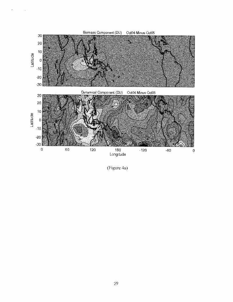
6 Impact of biomass burning during the 2006 El Niiio

In sections 4 and 5 we analyzed the El NiAo related changes in tropospheric O3 and CO in 2006

using both the model and observations. In this section we analyze the model results to estimate

the relatibe importance of biomass burning and large scale transport in producing the El Niiio

related changes in tropospheric 0 3 . Our approach is similar to the one used by C'hundru et al.

[2002] in analyzing the effect of the 1997 El NiHo on tropospheric 0 3 . The model was run in

two modes: The first mode explicitly included the NOx and CO emission rates associated with

the Indonesian fires as given in Table 1. The results of these runs are discussed in sections 4 and

5. In the second mode, the model was run by excluding the contributions from the Indonesian

fires. The model runs in this mode are used to assess the effects of large scale transport on

tropospheric O3 as shown in the bottom panels of Figures 4a-4c. The difference of the two runs

gives the contribution from biomass burning as shown in the upper panels of Figures 4a-4c.

In October 2006 the increase in O1 due to biomass burning is about 4-6 DU (Figure 4a, upper

panel). This increase is limited to a small region comprising the islands of Sumatra, Java and

Borneo in the Indonesian region. It is comparable to 4-8 DU increase caused by changes in

meteorological conditions (Figure 4b, lower panel). The latter, howeker, extends over a much

larger area in the Indian Ocean encompassing regions of the Indian subcontinent and south-east

Asia in the north, to western Australia in the south. These patterns are essentially similar in

November 2006 (Figure 4b). In December, 2006, the O3 increase due to biomass burning is

reduced to zero and the dynamical component of the O3 field is identical to Figure 2c (lower

panel).

Table 2 shows the model simulations of monthly averaged global tropospheric burden of CO, O3

and NOx with and without Indonesian fire emissions. The table shows that during October 2006

the Indonesian tires contributed about 36 Tg which was about 10.7% of the global budget of CO.

The increase in CO during November and December were respectively 12.6?41 and 8.1% of the

global budget. These changes are significant and suggest that the El Nifio related fires in the

Indonesian region may have contributed significantly to global pollution. In comparison the

impact of fire was relatively small (< 3%) on the global O3 burden. Logan et al. [2008] have

suggested NOx production due to lightning as a contributing factor to the positive anomaly in

TGO during December 2006. The NOx production due to lightning is implicitly included in the

model calculations. In the tropical Pacific region (1 2's- 12W, 90°E- 1 70°E), lightning produced a

total of 0.032 Tg NO in October 2006. This value increased to 0.0492 Tg NO in November and

0.0562 Tg NO in December 2006.

"7 The El Nifio of 2006: A long-term perspective

Though the main focus of this study is the El Nifio event of 2006, such events are very eequelal,

and may have simificant impact on global pollution. According to the World Meteorological

Organization (VCIYIO) an El Niiio (La Niria) event is identified when sea surface temperahre

(SST) in the Nifio 3.4 region (5'S-5%, 120°W-17Q0W) is at least OS°C above (below) normal

when averaged over three consecutive months. The relation between ASST and ATCO (the

difference in TGO between eastern and western Pacific) is shown in Figure 5. The ATCO time

series is derived by subtracting TGO in the eastern Pacific (1 5's- 15%, 135'W- 180') from TCO

in the western Pacific ( I 5 " S - 1 ~ ~ , 9j0E-140°E). The time series is deseasonalized and smoothed

with a three-month mn ing average to be compatible with Nil30 3.4 SST. TCO is derived from

29 years (1979-2008) of total column ozone measurements from Nimbus 7 TOMS, Earth Probe

TOMS and OM1 using the convective cloud differential (CCD) method leg., Ziemke et al.,

20051. Figure 5 shows a very robust correlation between ASST and ATCO. Exen though the

1997 El Nirio produced largest pel-turbations in SST and TCO in the tropical Pacific, El Nifio

events like 2006 are more common. They are also episodic. Before 1997 they occurred about

every 3-4 years, but more recently they have occusred every 2 years. A Erequent occurrence of

EI Nifio, similar to 2006, has the potential of increasing the global pollution triggered by the

dryness and the resulting forest fires in the Indonesian region.

8 Summary and Conclusion

We have studied the effects of the 2006 El NiAo on tropospheric 03, and CO at tropical and sub-

tropical latitudes measured from the BMI and MES instruments on the Aura satellite. The zonal

chsnracteristics o f ohsewed changes in these constiguents are similar to those regode8 by Loga~z et

a/. [2008] based on measwements of these cctnstihilents from the TES insmment on the same

satellite. During October and December 2006, both these studies revealed a dipole like structure

in TCO in the tropics with an increase over the western Pacific region and a decrease over the

eastern Pacific region. The dipole structure was weaker during November 2006.

The 2006 El NiAo-induced drought allowed forest fires to spread rapidly during October and

November in the Indonesian region. The effects of these fires are clearly seen in the

enhancement of CO concentration measured from both the MLS and TES instruments. We have

used a global model of atmospheric chemistry and transport (GMI CTM) to quantify the relative

importance of biomass burning and large scale transport in producing observed changes in TCO.

The model results show that during October and November both biomass burning and

meteorological changes contributed almost equally to increases in TCO in the Indonesian region.

The biomass component was 4-6 DU but it was limited to the Indonesian region where the fires

were most intense. The dynamical component was 4-8 DU but it covered a much larger area in

the western Pacific and Indian Ocean extending from South East Asia in the north to western

Australia in the south. During December 2006 the effect of biomass burning was reduced to zero

and the observed changes in TCO were mostly due to dynamical effects. C'l?undru et al. [2002]

have obtained similar results for the 1997 El NiAo using ozone measurements from Earth Probe

TOMS and comparing them with the GEOS-CHEM model. The 1997 El Nifio was significantly

stronger than the 2006 El NiAo and caused greater perturbations in TCO due to both forest fires

and large scale transport. For the 2006 El Niiio the model shows an increase of 2-3% in the

global burden of tropospheric ozone. In comparison, the global burden of CO increased by 8-

12%.

This study shows that the 2006 El NiAo can be characterized from long records of tropospheric

O3 and sea surface temperature as a moderate event, yet still the contribution to pollution from

biomass burning emissions over Indonesia was substantial, both locally and also uhen evaluated

on a global basis. In recent years El NiAo events have occurred with greater frequency than in

previous years dating back to 1979. Both the frequency and scale of emissions from biomass

burning suggests that even relatively moderate El NiAo events can be an important source of

pollution in the troposphere.

Acknowledgments. The authors thank the Aura OMI and MLS instrument and algorithm teams

IkPr the extensive satellite measurements used in this study. 'Fhe OM1 instrumc~at was bttilt by

Dutch-Finnish colfaboration, and is managed by the Royal Netherlands Meteorological Institute

(KNMI). The authors also thank the GMI processing group for their extensive efforts in

producing the GMI CTM. Data used in this study were processed at NASA Coddard Space

Flight Center. Funding for this research was provided in part by Goddard Earth Science

Technology (GEST) grant NGC5-494.

Appendix: Comparisons beween OMZMLS and model O3

Zienzke et al, [2006] compared tropospheric ozone variabiliv derived from OMIiNILS and the

GMI CTM using earlier versions of both the model and measurements. As discussed in section

2, the total ozone data used in this paper is based on the TOMS version 8.5 algorithm instead of

version 8 as used by Ziemke ef al. [2006]. The model also uses different emission sowces and

meteorological fields. In the following we compare the temporaliseasonal and zonal variability

of TCO fields derived &om the model and the measurements under varying conditions.

Figure A1 compares the temporal and seasonal variations of the model and obsewations for three

separate regions: American (left four panels), African (middle four panels), and Indonesian (right

four panels). In each region latitudes extend from north to south with the top panel being

northernmost. In nortliern latitudes tropospheric O3 for the model and measurement maximizes

around March-July. In southern latitudes largest amounts occur in September-November. In

between at low latitudes the seasonal variability is small in comparison. In general the temporal

vajriability in model and measurements are remarkably similar indicating the ability of the model

to capture month-by-month variability in the data. All three top panels in Figure A1 for the

latitude band 3O"N-35% show offset differences of 5-10 DU (with GMI larges than OMliMLS).

For the upper right panel in Figure A1 (corresponding to east China) the model and measured C13

in summer are comparable but the model values are larger than measured values by 5-10 DU in

winter and spring months when STE is greatest,

warti in ef al. [2002] and Chandra et. al. [ZOO21 compared the seasonal variability in eopospheric

O3 from the GEBS-Ckem model and TOMS GCD measurements. A large discrepancy was

fouind between the model and the CCD measurements over low latitudes in northern Africa

including Abidjan (5%, 4"W). The model indicated maximum trogospherie column O3 around

December-Febmary dwing peak time sf the biomass burning 'I-vhereas TOMS shollied greatest

amounts around June-October at a time when there is little or no biomass burning in northern

Africa. Our analysis shows that the OM1 measurements agree much better with model than the

TOMS measurements pertaining to this seasonal variability over Africa. The GMI model

indicates that enhancements in tropospheric 01 over northern Africa from the biomass burning

lie almost entirely below 500 hPa and are highly localized to the relatively small region of

burning emissions.

Figure A2 shows statistical comparisons of model and observations. The three panels in this

figure show their zonal correlations (top panel), mean zonal offset difference (middle panel) and

mean zonal RMS (lower panel). The grey shading in the top panel represents areas that are not

statistically significant at 99.9% confidence level. Figure A2 shows that the positive correlation

between the model and OMIIMLS TCO, extending out to mid-latitudes, drops to negative values

in higher latitudes. Several factors could contribute to near-zero or negative cross-correlations.

Aside from known model uncertainties which include STE, OM1 retrievals become less sensitive

in measuring tropospheric O3 in high latitudes (i.e., high solar zenith angles) and have reduced

sensitivity in measuring 0 3 in the lower troposphere, especially for high solar zenith angles and

large slant columns. The model and observations compare the best in the tropics and subtropics

extending out to latitudes of about k30" to lt35'. This is the latitude range chosen for GMI and

OMIMLS measurements for studying the 2006 El Niiio event.

References

Bloom, S., et al., Documentation and validation of the Coddard Earth Observing System (GEOS)

Data Assimilation System - Version 4, TechnicuE Report Series on Globcrl iModeling and Data

Assimilation 104606, 2005,

Ghandra, S., J. R. Ziemke, 1V. Min, and W. G. Read, Effects of 1997-1998 El Miiio on

tropospheric orone and water vapor, Ceop!~js. Ke,s. Lett., 25, 3867-3870, 1998.

Chandra, S., J. R. Ziemke, Tropical tropospheric ozone: Implications for dynamics and biomass

burning, J Geophjfs. Res., 107(D 141, doi: 10,10291200 1 JD000447,2002.

Ghandra, S., J. R. Ziemke, and R. V. Martin, Tropospheric ozone at tropical and middle latitudes

derived li-om TOMSMLS residual: Comparison with a global model, J Geuphy.~. Res,,

108(D9), 429 1, doi: 10.102912002JD0029 12,2003.

Chandra, S., J. R. Ziemke, M. R. Schoeberl, et al., Effects of the 2004 EX Nifio on tropospheric

ozone and water vapor, Geoph~/s. Res. Left., 34, L06802, doi: 10.10291204)6GL028779,2007.

Doherty, R. M., D. S. Stevenson, C. E. Johnson, et al., Tropospheric ozone and El Nirio-Southern

Oscillation: Influence of atmospheric dynamics, bion~ass buming emissions, and future climate

change, J. Geophys. lies., 11 1, D 19304, doi: 10,102912005 JD006849,2006.

Duncan, B. N., R. V. Martin, A. Staudt, et al., Inter-annual and seasonal variability of biomass

burning emissions constrained by satellite observations, J. Geophys. Res., 108,

doi: 10.1029/2082JD002378,2003.

Duncan, B., et al., Model Study of the Cross-Tropopause Transport of Biomass Burning

Pollution, Atmos. Chem. Phys., 7,37 13-3'736,2007.

Duncan, B., et al., The influence of European pollution on ozone in the Near East and northern

Africa, Atf~o.s. Clzem. Phys., 8, 2267-2283, 2008.

Froidevaux, L., Y. E3. Jiang, A. Lambert, et al., Validation of Aura Microwave Limb Sounder

stratospheric ozone measurements, J Geophys. Rex.. l f 3(D 1 5), D 1 5S20,2008.

Fadcjiwara, IM., K. Mita, S. Kawakami, et al., Tropospheric ozone enhancements dwing the

Indonesian -forest fire events in 1994 and in 1997 as revealed by ground-based observations,

Geophy.~. Res. Let&, 26,24 1 7-2420, 1999.

Guenther, A., T. Karl, P. Harley, et al., Estimates of global terrestrial isoprene emissions using

MEGAN (Mode2 s f Emissions of Gases and Aerosols from Natt~re), Atmos. Chern. PhyYr., 6,

3188-32B0,2006.

Jacobson, M., Computaton of global photochemistry with SMVGEAR 11, Atmos. Environ., 29,

354 1-2536, 1995.

Kroon, M., I. Petropavlovskikh, R. E. Shetter, S. Hall, K. Ullmann, J. P. Veefkind, K. D.

McPeters, E. V, Browell, and P. Levelt, OM1 Total Ozone Column Validation with Aura-AVE

CAFS Observations, J. Geophys. Rex, 113(D16), Dl 5S 13, doi: 10.1029/2007J1)008795,2008a.

Kroon, M., J. P. Veeikind, M. Sneep, R. D. McPeters, P. K. Bhartia, and P. Levelt, Comparing

OMI-TOMS and OMI-DOAS total ozone column data, J. Geophys. Re.s., 113(D 16), D 16S28,

doi: 10.1029/20075D008798,2008b.

Levelt, P. F., et al., Science objectives of the Ozone Monitoring Instrument, IEEE Truns.

Geophys. Remote Sens., 44(5) 1 199- 1208,2006.

Livesey, N. J., M. J. Filipiak, L. Froidevaux, et al., Validation of Aura Microwave Limb Sounder

0 - 3 and CO observations in the upper troposphere and lower stratosphere, Geophys. Res.,

113(D15), D15S02,2008.

Logan, J. A., I. Megretskaia, R. Nassar, et al., Effects of the 2006 Elo Niiio on tropospheric

composition as revealed by data from the Tropospheric Emission Spectrometer (TES), Geophys.

Rw. Lett., 35, L03816, doi: 10.102012007GL03 1698, 2008.

Martin, R.V., D.J. Jacob, J.A. Logan, et al., Interpretation of TOMS observations of tropical

tropospheric ozone with a global model and in-situ observations, J. Geophys. Res,, 107(1)18),

435 1 , doi: 10.102912001 JDO01480, 2002.

McPeters, R. D., M. Kroon, G. J. Labow, E. Brinksma, D. Balis, I. Petropavlovskikh, J. P.

Veefkind, P. K. Bhartia, and P. Levelt, Validation of the Aura Ozone Monitoring Instrument

Total Column Ozone I'roduct, J. Geophys. Res., 113(D1 S), D 15S 14,

doi: 10.1029i2007JD008802,2008.

Peters, W., &I. Krol, F. Dentener, et al., Identification of an El Nino-Southern Oscillation signal

in a multiyear global simulation of tropospheric ozone, J. Geophys. RP~Y., 106(Dl0), 10,398-

10,402, 200 1.

Schoeberl, M. R., B. N. Duncan, A. Douglass J. Waters, N. Livesey, W. Read, M. Filipiak, The

Carbon Monoxide Tape Recorder, Geophys. Res. Lett., 10.102912006GL026 178,2006.

Schoeberl, M. R., J. R. Ziernke, B. Bojkov, N. Livesy, B. N. Duncan, et al., A trajectory-based

estimate sf the tropospheric ozone column using the residual method, 4: Geopkvs. Res., 112,

D24S49, doi: 10.1029/200751)008773,2007.

Strahan, S.E., B.N. Duncan and P. I-loor, Obsemationally-derived diagnostics of transpod in the

lowermost stratosphere and their application to the GMI chemistry transport model, Atmos.

G e m . PA-vs., 7,2435-2445,2007.

Sudo, K., and M. Takahashi, Simulation o f tropospheric ozone changes during 1997- 1998 El

Niiio: Meteorological impact on tropospheric photochernistl-y, Geophys. Res. Lett., 28, 4091-

4094,200 1.

Thompson, A. M., J* C. Witte, R. D. Hudson, et al., Tropical tropospheric ozone and biomass

burning, Science, 291,2 128-2 132,2001.

Zeng, G., and J. A. Pyle, Influence of EI NiBo Southern Oscillation on stratosphereitroposphere

exchange and the global tropospheric ozone budget, Geophys. Res., Lett., 32, L01814,

doi: 10.1 02912004GL02 13 53,2005.

Ziemke, J. R., S. Chandra, and P. IS. Bhartia, A new NASA data product: Tropospheric and

stratospheric column ozone in the tropics derived from TOMS measurements, Bull. Amer.

Meteorol. SOC., 81, 580-583,2000,

Z i e d e , J. R., S. Chandra, and P. K. Bhartia, A 25-year data record of atmospheric ozone &om

TOMS Cloud Slicing: Implications for trends in stratospheric and tropospheric ozone, J.

Geophys. Res., 110, D15 105, doi: 10.102912004JD005687,2005.

Ziernke, J.R., S. Chandra, 13. N. Duncan, L. Froidevaux, P. ti. Bhartia, P. F. Levelt, and 1. W.

Waters, Tropospheric ozone detemined from Ama OM1 and MLS: Evaluation of measurements

and coqarison with the Global Modeling Initiative's Chemical Transport Model, J. Geopbs.

Res., 'L O.'L029/2006J&s007089,2006.

Table 1: Emissions of CO and NO for 2006.

July

September I 18.3 99 0.32 6.8

August

October

16.6 103 0.29 7.4

"Biomass burning emissions only.

November

b~missions from all sources, including fossil fuels, biofuels, and biomass burning, except

biomass burning from Indonesia.

6.3 79 0.1 1 6.3

Table 2. Monthly Averaged Global Tropospheric Burden of 60, 03, and NOx for the Model.

Indonesia

No Indonesia

ACO

AGO (94)

Indonesia

No Indonesia

A 0 3

AQ7 (%)

Indonesia

No Indonesia

AMOx

ANOx 6%)

Sep. Oct. Mov, Dec.

Simulations with ("Indonesia") and without ("No Indonesia") the 2006 Indonesia fire emissions.

Figure Captions.

Figure 1. (a) Tropospheric column ozone measured in DU from OMIiMLS for October 2004

(top panel), October 2005 (middle panel), and October 2006 (bottom panel). (b) Same as (a) but

instead for the GMI model. (c) The difference (GMI minus OMI/MLS) between Figure l a and

Figure lb.

Figure 2. (a) Inter-annual difference (October 2006 minus October 2005) of tropospheric

column ozone measured in DU from OMIIMLS (top panel) and the GMI model (bottom panel).

(b) Same as (a) but instead for November. (c) Same as (a) but instead for December.

Figure 3. (a) Inter-annual annual difference (October 2006 minus October 2005) of 215 hPa GO

from MLS (top panel) and 227 hPa CO from the GMI model (bottom panel). All quantities

represent volume mixing ratio in units ppbv. (b) Same as (a) but instead for November. (c)

Same as (a) but instead for December.

Figure 4. (a) Inter-annual difference (October 2006 minus October 2005) of GMI tropospheric

column ozone (in DU) of the Indonesia biomass burning component (top panel) and the

dynamically driven component (bottom panel). (b) Same as (a) but instead for November. (c)

Same as (a) but instead for December.

Figure 5. OMI/MLS time series ATGO (dark curve) plotted with Nifio 3.4 time series ASST

(light curve). ATCO is measured in DU while ASST is in Celsius degrees and was multiplied by

a factor of three for scaling with ATCO. The ATCO time series is derived by subtracting TCO in

the eastern Pacific (1 5 " ~ - 15%, 135"W- 180") from TCO in the western Pacific (1 5"s- 15"N, 95"E-

140"E). The ATCO time series was deseasonalized and was also smoothed with a three-month

running average to be compatible with the Nifio 3.4 time series.

Figure Al . Monthly time series comparisons of GMI (dotted curves) and OMIMLS (solid

curves) tropospheric column O3 (in DU) for three separate regions: American (left four panels),

African (middle four panels), and Indonesian (right four panels).

Figure 8 2 . (top) Zonal correlations between BMIIMLS and GMl tropospheric column eb3.

(middle) Calculated mean zonal offset difference (CMI minus OMIMLS) measured in DU

between model and obsewation. (bottom) Calculated zonal RIMS of difference (GMI minus

OMIMLS) in DU. For both model and obsewation, fields for similar months (January - December) from 2004 to 2006 where averaged together to derive mean 12-month latihrde-

longitude gridded distributions of tropospheric Oj. All statistical calculations were done zonally

for each latitude band using the 72 gridded longitudinal values from model and obsewation.

0 60 120 1 80 -1 20 - 60 0 Longitude

(Figure la)

GMI 03 (DU) October 2006

0 60 120 1 80 -1 20 - 60 0 Longitude

0 60 120 1 80 -1 20 - 60 0 Longitude

(Figure lc)

GM I Tro~osxdleric Column Ozone IDU) Od06 Minus Od05

0 6 0 120 180 -120 -60 Long~tude

(Figure 2a)

" Longitude

(Figure 2b)

OMMLS Trooodenc Column Ozone IDU) Dec06 M~nus DecO5

0 8 0 120 180 -120 -60 Longitude

(Figure 2c)

Longitude

(Figure 3a)

0 60 120 180 -120 -60 0 Longitude

(Figure 3 b)

Longitude

(Figure 3c)

0 60 120 180 -120 -60 0 Longitude

(Figure 421)

0 60 120 180 -120 -60 0 Longitude

(Figure 4b)

79 81 83 85 87 89 91 93 95 97 99 01 03 05 07 Year

(Figure 5)

Longrtude

(Figure 3b)

Thic . I I r r

Year

(Figure 5)

J F M A M J J A S O N D

-60 J F M A M J J A S O N D

Zonal RMS of Difference Betwpn OMllMLS and GMl I

-60 J F M A M J J A S O N D

Month

(Figure A2)