the case for investing in agriculture · the case for investing in agriculture ... the benefits of...
TRANSCRIPT

The case for investing in agriculture
MACQUARIE AGRICULTURAL FUNDS MANAGEMENT

2
DISCLAIMER
This document does not constitute financial product advice and should not be relied upon as such. The information in this document is for discussion purposes only and is not an offer or solicitation to purchase or sell any securities or financial product. None of the information in this document takes into account any person’s personal objectives, financial situation or needs and you must determine whether the information is appropriate in terms of your particular circumstances. We recommend you obtain financial, legal and taxation advice before making any financial investment decision.
The information contained in this document is strictly confidential. If you are not the intended recipient, you may not disclose or use the information in this document in any way. No liability is accepted for any unauthorised use of the information contained in this document.
This document is not to be distributed to any person or corporation by the recipient. Macquarie Group Limited is the owner of the copyright material in this document unless otherwise specified. Macquarie Group Limited and its worldwide affiliates and subsidiaries accept no liability whatsoever for any direct, indirect, consequential or other loss arising from any use of this document and/or further communication in relation to this document.
This document has been prepared based on information believed to be accurate at the time of the preparation of this document. Subsequent changes in circumstances may occur at any time and may impact the accuracy of the information in this document. Some of the information in this document and the figures that have been quoted, and or used within it, have yet to be confirmed and finalised and consent has not been obtained from all relevant stakeholders. It is important to note that to this extent the document may not be accurate or complete and some of the information could be subject to amendments.
Any forecasts contained in this document are predictive in character and therefore no undue reliance should be placed on the forecast information. Whilst every effort has been taken to ensure that the assumptions on which the forecasts are based are reasonable, the forecasts may be affected by incorrect assumptions or by known or unknown risks and uncertainties. The actual results may differ substantially from the forecasts and some facts and opinions may change without notice on the basis of changing market conditions.
Past performance is no indication of future performance.
Other than Macquarie Bank Limited ABN 46 008 583 542 (MBL), no Macquarie Group entity mentioned in this document is an authorised deposit-taking institution for the purposes of the Banking Act 1959 (Cth) and their obligations do not represent deposits or other liabilities of MBL. MBL does not guarantee or otherwise provide assurance in respect of the obligations of the Macquarie Group entities mentioned in this document.
Executive summary 01
Demand and supply fundamentals – a structural shift 02
The benefits of investing in agricultural assets 10
Making returns from agriculture 12
Conclusion and footnotes 16
Contents

1
Executive summary
The price rises in agricultural commodities which occurred through 2007 and 2008 brought attention to the market dynamics and the drivers of demand and supply for these commodities. There is now increased importance placed on the issue of food security and recognition that trends have developed which have the potential to lead to further, long term price rises in these markets.
Agricultural commodities have three main uses – food, feed and fuel – and demand for each of these uses is increasing. This increase is being driven by global population growth (increasing demand for food), economic growth in emerging markets (demand for feed) and biofuel policies which are being implemented by governments across the globe (demand for fuel).
Whilst this is occurring, increasing supply is becoming more troublesome. The amount of high quality arable land available is under pressure due to urbanisation, land degradation and climate change and, as a result, the global harvested area for key agricultural crops has increased only modestly over recent years. At the same time, growth in global crop yields is decreasing and the ability to increase yields is being impacted by climate change, water scarcity and the reluctance to adopt genetically modified crops. Even if the third factor is overcome, some evidence suggests that the use of these crops doesn’t always cause an increase in yields.
There is no short term solution to overcoming this shifting dynamic and to do so would require a long term, coordinated, global effort to find new solutions. This is what occurred during the Green Revolution, but as stated by Jacques Diouf replicating this effort could be a lot more difficult this time around.
In the lead up to the price spikes of 2008, the long-term demand factors were joined by a set of short-term factors to create a ‘perfect storm’ for agricultural commodity prices. Despite
a severe fall in prices following these spikes, the prices of many commodities have now stabilised above historical levels.
Agricultural assets provide investors with an investment which acts as a hedge against inflation, has low correlations to traditional asset classes and is less impacted by economic slowdowns. In order to gain exposure to this asset class investors can invest directly via agricultural assets (such as land, livestock and crops) or indirectly through listed equities and futures.
The most direct and pure exposure is achieved through investing in real agricultural assets and gaining exposure to farming operations and the underlying land. Listed equities have the advantage of providing liquidity, but are more highly correlated to equity markets, while futures provide a shorter term exposure to price volatility, rather than exposure to the long term fundamentals.
Agricultural investments are exposed to a number of risks, such as drought, pests, disease, desertification, fire, commodity price volatility and political risks. Although it is impossible to remove some of these risks (for example, drought) these risks can be mitigated through good management practices and a sound investment strategy. Geographic and commodity diversification reduce the impact of environmental factors and commodity price volatility, while the adoption of various technologies and management techniques by farm managers can reduce the risks associated with fire, pests and disease.
Finally, it has been shown that achieving scale in agriculture results in reduced volatility in farming returns, due to the benefits scale provides. These include the ability to acquire a portfolio of diversified assets, to negotiate lower unit costs of production, to invest in technology and to acquire highly experienced management teams, as well as providing access to capital for continued growth.
"We not only need to grow an extra one billion tonnes of cereals a year by 2050… but do so from a diminishing resource base of land and water in many of the world’s regions, and in an environment increasingly threatened by global warming and climate change.1”
Jacques Diouf, Director General, Food and Agriculture Organization of the United Nations (FAO)

2
Demand and supply fundamentals – a structural shift
The price rises in agricultural commodities witnessed in 2007 and 2008 brought attention to the structural shift that has been developing in the demand and supply dynamic for these commodities for some time. There is now a growing recognition of the factors that gave rise to these price rises and a realisation that trends have developed which have the potential to deliver longer term, positive price movement for agricultural commodities.
Demand for all uses of agricultural commodities is increasingAgricultural commodities have three main uses: food, feed and fuel. Demand for each of these uses is increasing, putting pressure on supply to meet this demand. The key drivers of this increase in demand are:
Global population growth – increased population ■
results in increased demand for food;
Economic growth in emerging markets – ■
increased GDP per capita and urbanisation are resulting in increased demand for meat and dairy products leading to increased demand for livestock feed; and
Biofuel policies – government policies which ■
set targets for renewable fuels are resulting in the diversion of agricultural output to biofuels.
Global population growth
Population growth is a basic factor that drives an increase in the consumption of agricultural products, as the growing global population is the core base of demand growth for food. The global population has grown substantially over the past few decades, and from its current base of 6.1 billion people, is projected to rise to 8.3 billion by 2030 and 9.1 billion by 2050, resulting in an additional 79 million mouths to feed each year.
Further, in the coming years, population growth is expected to be concentrated in developing and emerging economies, meaning that some countries that have previously been self sufficient will need to start importing foods.
Although, the rate of growth is slowly decelerating, the absolute annual increases are undeniably large. Growth in food demand is reflected in the
growth in demand for wheat, which is one of the primary food grains. Human consumption accounts for approximately 70 per cent of total wheat consumption and, according to the USDA, over the past 20 years worldwide wheat consumption has been growing, on average, at 1 per cent per annum.2
Economic growth in emerging markets
Economic growth in the emerging markets is a source of growth in the demand for agricultural products, as rising per capita incomes and urbanisation are resulting in greater consumption of food, as well as a shift in the dietary patterns in these countries.
Rising GDP per capita and incomes are important drivers of demand growth for agricultural products. As GDP and incomes grow people consume more, but more importantly consumers trade up to higher value foods, such as meat and dairy, as they become wealthier. This change in dietary habits is most pronounced in emerging economies, which is significant because these economies are expected to experience the strongest economic growth going forward.
Urbanisation is also closely linked to economic growth and rising incomes. The factors that underpin urbanisation include the search for employment or higher paying employment, access to better health and education services, and greater entertainment and lifestyle options. Urbanisation often leads to
Figure 1: Global population
1950
1960
1970
1980
1990
2000
2010
2020
2030
2040
2050
10
Billio
ns
9
8
7
6
5
4
3
2
1
■ More developed regions ■ Less developed regions■ Least developed countries
Source: UN Secretariat

3
Figure 3: Growing urban population
1950
1960
1970
1980
1990
2000
2010
2020
2030
2040
2050
10
Billio
ns
■ Rural population ■ Urban population
9
8
7
6
5
4
3
2
1
0
Source: UN Department of Economic and Social Affairs
are most likely to come from intensive production systems in which animals are raised in confinement systems* and reared, to a large extent, on grains. This has an important multiplier effect on grain consumption due to the increased demand for grains which are used as feed for livestock.
To produce one gram of animal weight requires multiple grams of grains to be used as feed. For example, approximately 8.3 grams of grain are required to produce 1 gram of beef, while 3.1 grams of grain are required for 1 gram of pork. Further, the energy produced by one gram of beef is 2.78 kcal, This is much less than the energy produced by the 8.3 grams of grain required to produce it, which is approximately 25 kcal. This multiplier effect means that as dietary patterns shift to include a greater proportion of higher value foods a much greater volume of grains is required to maintain the amount of energy consumed.
a higher per capita income and an increase in living standards which, in turn, results in urban populations consuming a higher number of calories per capita than their rural counterparts and, generally, demanding better quality and a greater variety of food products.
It is estimated that nearly 600 million people in the Asia-Pacific region will move from rural areas to cities by 20203 and by 2030 the number of people living in cities is forecast to grow to 60 per cent of the world’s population, up from around half currently.
As mentioned above, the key change in dietary patterns resulting from increases in GDP, income and urbanisation is the trade up from lower-value foods, such as staple grains, to higher value foods, such as meat, eggs, fish and dairy products.
As arable land available for farming diminishes, substantial gains in production of higher value foods
Table 1: Grains required for animal production
Beef Pork Poultry FishGrains required per gram of animal weight (g) 8.3 3.1 2.0 1.5
Energy yield per gram of meat (kcal) 2.78 3.76 2.13 1.16
Grains required per kcal of energy provision to human 2.99 0.82 0.94 1.29
Source: Goldman Sachs Research
Figure 2: GDP and food consumption
4,000
Prot
ein
Cons
umpt
ion
(kca
l/cap
ita/d
ay)
GDP per Capita (USD/capita)
3,500
3000
2,500
2,000
1,500
1,00010,000 20,000 30,000 40,000 50,000
Source: FAO, IMF (2003)
* The practice of raising livestock in confinement, at high stocking density, where a farm operates as a factory. The main products of this industry are meat, milk and eggs for human consumption.

4
China – Increasing GDP, increasing demand for pork, increasing soybean imports
Over the past decade China’s GDP growth has averaged 12 per cent p.a.4, while their urban population has grown from approximately 450 million (36 per cent of total population) to over 600 million (45 per cent)5. As a result, meat consumption is increasing, as demand from this growing urban population increases and diets shift towards higher value products. Between 2000 and 2009 per capita consumption of pork grew from 31.2 kilograms to 36.4 kilograms6. In addition, the Chinese government has major initiatives underway to grow pig herds, as pork has become a staple of the Chinese diet comprising 60 per cent of total meat intake in 20077.
This increased demand for livestock has an accelerating effect on demand for animal feed, as pigs are unable to digest grass and therefore must be fed a grain intensive diet. Approximately three grams of grain are required to produce one gram of pork meaning as the demand for pork rises, so does the demand for feed8.
Soybean meal is an ideal feed ingredient for commercially raised hogs due to its protein content and its wide availability. The demand for soybeans and soybean meal in China has increased and China is now the world’s largest consumer and importer of soybeans, with up to 63 per cent being crushed and used as livestock feed.
Domestic soybean supply can no longer keep up with China’s rapid growth in consumption and land and water constraints are restricting local production growth. The overall effect is a shift in China’s soybean market dynamics.
China is a major consumer of pork globally, accounting for 47 per cent of global consumption in 2008/09. As pork consumption continues to grow in China further increases in demand for soybeans and additional reliance on imports are expected.
Figure 4: China’s soybean market dynamics Figure 5: Domestic pork consumption
1998
/99
1999
/00
2000
/01
2001
/02
2002
/03
2003
/04
2004
/05
2005
/06
2006
/07
2007
/08
2008
/09
Prod
uctio
n &
cons
umpt
ion
(’000
MT)
Impo
rts (’
000
MT)
60,000
50,000
40,000
30,000
20,000
10,000
45,000
30,000
37,500
22,500
15,000
00
7,500
■ Imports
Production
Domestic consumption
1980
/81
1982
/83
1984
/85
1986
/87
1988
/89
1990
/91
1992
/93
1994
/05
1996
/97
1998
/99
2000
/01
2002
/03
2004
/05
2006
/07
2008
/09
Cons
umpt
ion
(100
0 M
T CW
E)
120,000
100,000
80,000
60,000
40,000
20,000
0
■ World ■ China
Source: USDA Source: USDA
Demand and supply fundamentals – a structural shift

5
The expansion of the biofuel industry results in the diversion of increasing quantities of cereal, sugar, oilseeds and vegetable oils away from their traditional uses as food and animal feed. The diversion effect of biofuels can already be witnessed in the uses for corn in the US. Since 2002, when the USDA’s World Agricultural Supply and Demand Estimates (WASDE) report began including corn consumption for ethanol, the share of corn devoted to ethanol production has risen from less than 10 per cent to the almost 30 per cent projected for the 2009–10 season.
Figure 6: US corn market
1998
/99
1999
/00
2000
/01
2001
/02
2002
/03
2003
/04
2004
/05
2005
/06
2006
/07
2007
/08
2008
/09
2009
/10
Bush
els
(milli
ons)
■ Feed and residual ■ Food, seed and other industrial ■ Exports ■ Ethanol for fuel
Production
14,000
12,000
10,000
8,000
6,000
4,000
2,000
0
Source: Macquarie, USDA
Diversion of output to biofuels
Until recently, demand for agricultural commodities was driven by the demand for food and demand for feed. However, the search for alternative, renewable sources of energy has introduced a third competing use in biofuels. Although, only 4 per cent of global grain and oilseeds were used in the production of biofuels in 2007 and 2008, the recent growth in biofuel production is providing an additional and relatively new driver on the demand side for agricultural commodities.
The two most accessible biofuels are ethanol and biodiesel. Ethanol is produced from a range of agricultural sources including corn, wheat and sugar, while biodiesel is manufactured from oilseed feed stocks, most commonly rapeseed (canola) oil and soybean oil.
The increase in the use of biofuels has resulted from a number of government policies around the world (such as the Renewable Fuel Standard Program in the US) setting targets for the use of renewable fuels. More than forty countries have established policies aimed at promoting the use of biofuels and biodiesel. These policies are expected to have significant impact on the demand for biofuels and the associated inputs, with world ethanol production expected to double from 2008 levels to reach 127 billion litres a year by 2017, while biodiesel production is expected to expand from 11 billion litres in 2007 to about 24 billion litres in 201710.
Biofuel policies
A number of countries currently have policies aimed at increasing the use of biofuels and decreasing reliance on fossil fuels. These are expected to be a significant driver of demand for agricultural commodities in the coming years. Some examples of these policies are set out below.
Country/Country Grouping Targets
Brazil Mandatory blend of 20-25% ethanol with petrol, minimum blending of 3% biodiesel to diesel by July 2008 and 5% (B5) by end of 2010 and 5% (B5) by end of 2010
Canada 5% renewable content in petrol by 2010 and 2% renewable content in diesel fuel by 2012
China 15% of transport energy needs through use of biofuels by 2020
France and Germany 5.75% by 2008, 7% by 2010, 10% by 2015 (voluntary), 10% by 2020 (mandatory EU target)
India Proposed blending mandates of 5-10% for ethanol and 20% for biodiesel
Italy 5.75% by 2010 (mandatory), 10% by 2020 (mandatory EU target)
Japan 500 000 kilolitres, as converted to crude oil by 2010 (voluntary)
UK 5% biofuels by 2010 (mandatory), 10% by 2020 (mandatory EU target)
US 9bn gallons by 2008, rising to 36bn gallons by 2022 (mandatory). Of the 36bn gallons, 21bn to be from advanced biofuels (of which 16bn from cellulosic biofuels)
EU 10% by 2020 (mandatory)
Source: DB Climate Change Advisers

6
Supply factors are constrainedTo meet this increasing demand supply needs to increase. Supply is a function of acreage and yield and can only increase through an increase in one or both of these factors. However, the ability to increase yield and acreage is becoming more and more difficult due to the reasons addressed below.
Reducing availability of arable land
The global harvested area for key agricultural crops has increased only modestly over recent years and between 1961 and 2007 arable land grew at an average annual growth rate of 0.2 per cent 11. In addition, over this period Europe and Northern America experienced contractions in the arable land available for agricultural production. In Europe arable land declined by 0.9 per cent annually, while in Northern America the annual decline was 2 per cent 12. On a per capita basis, over this period, arable land globally has decreased by almost half.
Figure 7: Arable land per capita
0.6
0.7
0.8
■ Americas ■ Europe ■ Africa ■ World ■ Asia
0.5
0.4
0.3
0.2
0.1
1961
1963
1965
1967
1969
1971
1973
1975
1977
1979
1981
1983
1985
1987
1989
1991
1993
1995
1997
1999
2001
2003
2005
2007
Source: FAO
The amount of high quality arable land available is under pressure, due to:
rapid urbanization; ■
accelerating land degradation; and ■
climate change. ■
Urbanisation affects the availability of land, as cities are often built on prime farmland, and nutrients are therefore being transferred from farms to cities with little or no return flow. Urban areas become the source of sewage flows, run-off and other forms of waste that become environmental problems, often affecting surrounding rural areas. For example, in previous years in the US about 400,000 ha of farmland was lost to urbanization annually, while China lost about 5 million ha of farmland to urbanization during the period 1987–9213.
In addition, it has been estimated that 23 per cent of all usable land† on Earth has been affected by degradation to a degree sufficient to reduce its productivity. Land degradation occurs in many forms, including chemical contamination, soil erosion, nutrient depletion and salinity.
Finally, according to some estimates, world agricultural output could decrease by as much as one-sixth by 2020 due to climate change. The increased risk of droughts and floods and environmental damage as a result of climate change could leave large areas of land unsuitable for crops or grazing.
At present agricultural commodities compete for acreage on a global scale with each other. As there is limited arable land available, increasing production of one crop often results in a decrease in the production of another. In order to meet demand in the future more land will need to be brought into production and this will require farmers to push out to new frontiers. This shift into new frontiers gives rise to a number of issues. Firstly, this land is not always prime agricultural land and can lack the necessary infrastructure. As a result, it can require several years of investment to make the land cultivable and develop the necessary infrastructure. In addition, these areas can be located in areas of high environmental sensitivity and bringing this land into production can often be met by resistance from environmentalists. Finally, there may be arable land available in countries of high political risk, such as Zimbabwe. These political risks can prevent farmers entering these areas and bringing more land under cultivation.
Demand and supply fundamentals – a structural shift
† Usable land excludes areas such as mountains and deserts, for example
7
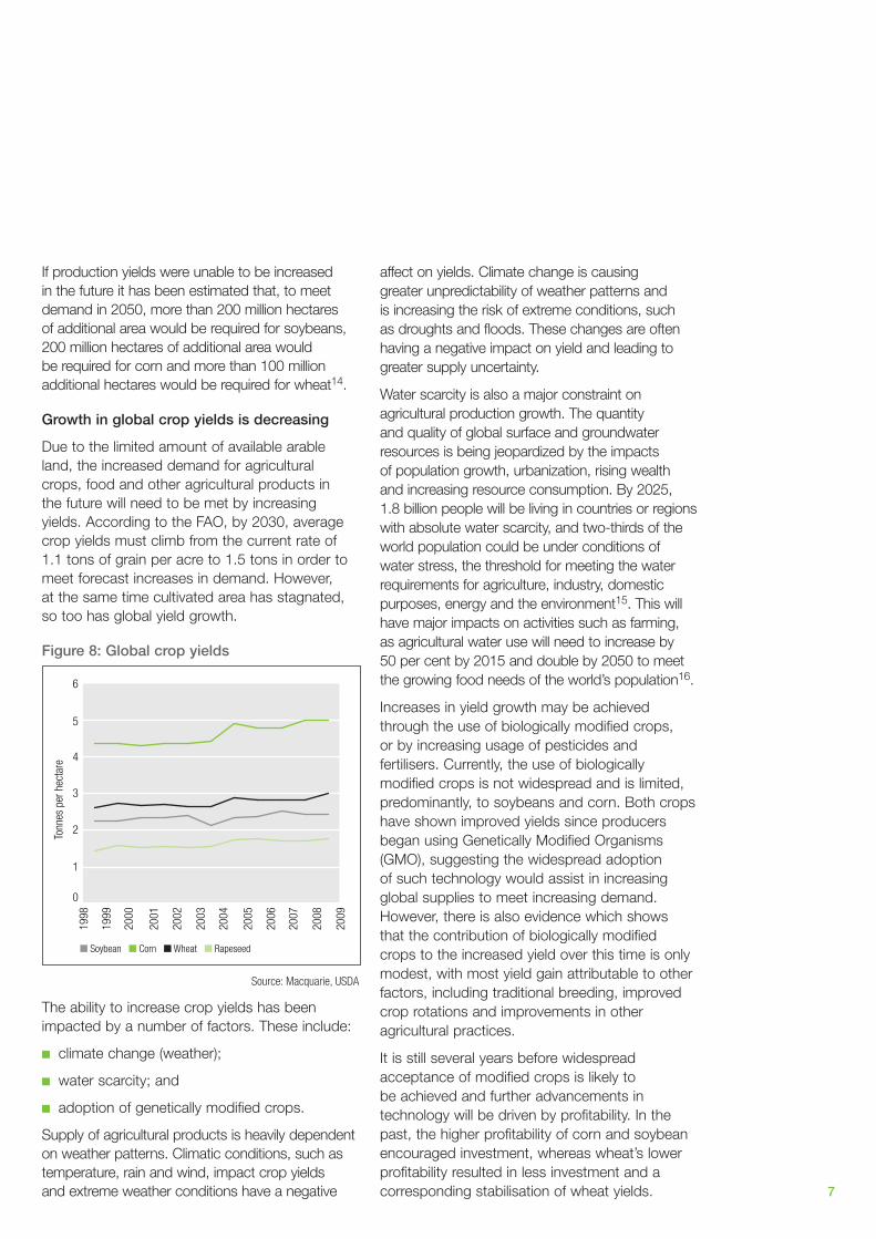
If production yields were unable to be increased in the future it has been estimated that, to meet demand in 2050, more than 200 million hectares of additional area would be required for soybeans, 200 million hectares of additional area would be required for corn and more than 100 million additional hectares would be required for wheat14.
Growth in global crop yields is decreasing
Due to the limited amount of available arable land, the increased demand for agricultural crops, food and other agricultural products in the future will need to be met by increasing yields. According to the FAO, by 2030, average crop yields must climb from the current rate of 1.1 tons of grain per acre to 1.5 tons in order to meet forecast increases in demand. However, at the same time cultivated area has stagnated, so too has global yield growth.
Figure 8: Global crop yields
1998
1999
2000
2001
2002
2003
2004
2005
2006
2007
2008
2009
6
Tonn
es p
er h
ecta
re
■ Soybean ■ Corn ■ Wheat ■ Rapeseed
5
4
3
2
1
0
Source: Macquarie, USDA
The ability to increase crop yields has been impacted by a number of factors. These include:
climate change (weather); ■
water scarcity; and ■
adoption of genetically modified crops. ■
Supply of agricultural products is heavily dependent on weather patterns. Climatic conditions, such as temperature, rain and wind, impact crop yields and extreme weather conditions have a negative
affect on yields. Climate change is causing greater unpredictability of weather patterns and is increasing the risk of extreme conditions, such as droughts and floods. These changes are often having a negative impact on yield and leading to greater supply uncertainty.
Water scarcity is also a major constraint on agricultural production growth. The quantity and quality of global surface and groundwater resources is being jeopardized by the impacts of population growth, urbanization, rising wealth and increasing resource consumption. By 2025, 1.8 billion people will be living in countries or regions with absolute water scarcity, and two-thirds of the world population could be under conditions of water stress, the threshold for meeting the water requirements for agriculture, industry, domestic purposes, energy and the environment15. This will have major impacts on activities such as farming, as agricultural water use will need to increase by 50 per cent by 2015 and double by 2050 to meet the growing food needs of the world’s population16.
Increases in yield growth may be achieved through the use of biologically modified crops, or by increasing usage of pesticides and fertilisers. Currently, the use of biologically modified crops is not widespread and is limited, predominantly, to soybeans and corn. Both crops have shown improved yields since producers began using Genetically Modified Organisms (GMO), suggesting the widespread adoption of such technology would assist in increasing global supplies to meet increasing demand. However, there is also evidence which shows that the contribution of biologically modified crops to the increased yield over this time is only modest, with most yield gain attributable to other factors, including traditional breeding, improved crop rotations and improvements in other agricultural practices.
It is still several years before widespread acceptance of modified crops is likely to be achieved and further advancements in technology will be driven by profitability. In the past, the higher profitability of corn and soybean encouraged investment, whereas wheat’s lower profitability resulted in less investment and a corresponding stabilisation of wheat yields.
Demand and supply fundamentals – a structural shift

8
Why is it different this time? This issue was first identified in 1798 by Thomas Malthus who proposed that “the power of population is indefinitely greater than the power in the earth to produce subsistence for man.” Malthus concluded that, should it remain unchecked, population growth would occur at a much greater rate than the growth in food supply and this would lead to famine and poverty throughout the world.
The issue of feeding the population is not new and in the past new techniques and technology allowed production to increase to meet the demands of the growing population, as was seen through the Green Revolution. However, the key differences today compared with the past are the additional demand being generated by biofuels and the difficulties faced in increasing supply.
The unlikelihood of a second Green Revolution
There is no short term solution to increasing supply and to do so would require a long term, coordinated, global effort to find new solutions. This is what occurred during the Green Revolution.
The Green Revolution refers to the transformation of agricultural practices that began in Mexico in the 1940s and resulted in increased food production to meet increased demand. Changes included:
the use of higher yielding strains of wheat, rice, ■
maize and other cereals;
higher use of hydrocarbon-based pesticides ■
and fertilisers; and
increased investment in dams, reservoirs and ■
canals allowing previously rain-fed land to be irrigated.
The combined effort and the advances of the Green Revolution allowed the world to keep pace with global population growth and, at the same time, provided the platform to increase calorie consumption per day in developing countries by about 25 per cent17.
Difficulty in replicating the Green Revolution stems from a number of factors. Today, increasing the use of fertilisers and chemicals is not only constrained by rising input costs, but also by the
need for ‘greener’ production techniques. Climate change, urbanisation and expansion of industry are making water increasingly scarce, reducing the ability to improve irrigation, while the wide spread acceptance of genetically modified crops is still many years away. Moreover, there is a considerable reduction in the sort of combined effort witnessed in the 1950s and 1960s to increase productivity. Since the 1980s public investment in farm science has stalled, with a sample of 21 first-world countries revealing that real public spending on agricultural research and development had reversed its previously upward path and began to decline at an annual rate of 0.6 per cent in the 1990s18.
In 2006, FAO Director General Jacques Diouf called for a second Green Revolution, but admitted that it may not be easy to replicate. He expressed that not only is there a need to increase production by an extra one billion tonnes of cereals per year by 2050, but that this needs to be achieved using a diminishing resource base of land and water and in an environment increasingly threatened by global warming and climate change.
Why won’t prices revert to historical levels?
Global agricultural commodity prices are cyclical and between 2006 and 2008 average world food prices grew dramatically. From the start of 2006 to early 2008, the price of rice rose by 217 per cent, wheat rose by 136 per cent, corn by 125 per cent and soybeans by 107 per cent. Almost just as swiftly, the price bubble came to an end with the abrupt slowdown in the global economy. Slowing GDP growth, together with indications of high harvest yields in some crops, combined to drive prices down.
In the lead up to 2008, the long-term demand factors described earlier joined a set of shorter-term factors to create a ‘perfect storm’ for agricultural commodity prices.
Over the twelve months to September 2007, ■
world stock markets increased in value by 31 per cent, adding $14 trillion of new stock market wealth to the world economy in just a year19.
The declining US dollar exchange rate ■
made commodities cheaper for non-US dollar denominated consumers, as most commodities are priced in US dollars.
Demand and supply fundamentals – a structural shift

9
Government intervention
Food security and biofuels are two areas which are resulting in government intervention in agricultural markets which, in turn, impacts the supply of agricultural commodities on the global market.
Food security is becoming an increasingly important issue and in order to secure food at reasonable prices for their domestic populations governments are intervening in agricultural markets. This is what occurred in 2007 and 2008 when, faced with rising food prices, many countries adopted policy measures designed to reduce the impact on their domestic populations.
These policies are often ineffective, or even counterproductive, in addressing food security and the impact of high food prices. For example, export restrictions seeking to secure food for the domestic populations appear to be well-intentioned measures, however, these restrictions also contribute to the food supply shortage on the world market and consequently result in higher prices.
Added to these food security policies, the increased focus on renewable fuels has led a number of governments to implement policies mandating the use of biofuels. As countries attempt to implement these policies additional supplies of agricultural commodities will be diverted away from food and feed, while at the same time demand from these sources is increasing.
Demand for oil pushed crude oil prices ■
to new heights of USD140 per barrel by mid-2008, resulting in higher input costs for farmers, but also making biofuels and ethanol more competitive sources of fuel, even without subsidies.
Carryover stocks of major food crops at the ■
beginning of the 2008 harvest were equal to just 62 days of consumption, a near-record low.
Droughts in 2005–07 in major wheat-producing ■
countries such as Argentina, Ukraine and Australia had been well documented and prices became highly sensitive to news of possible supply shortages.
As grain stocks fell and higher prices affected ■
domestic food consumption, governments began implementing policies to secure their own domestic food security. Trade in over-the counter derivatives had ■
expanded to a level, that some suggest, was many times larger than trade in organised exchanges. Finally, speculation at some of the trading ■
desks of global banks and by index traders in commodity futures markets was also a factor.
These factors led commodity prices to over-reach until after July 2008, at which time the exchange rate of the US dollar began a short-term appreciation against other major currencies and energy prices collapsed. Despite a severe decline in prices, the fall in commodity prices has not been as dramatic as its rise and the prices of many commodities have stabilised at about 2007 levels.
The stabilisation of prices at above historical levels indicates that the shift in long term demand and supply factors is causing a structural shift in agricultural prices.
Demand and supply fundamentals – a structural shift

10
Investing in agricultural assets provides a number of benefits to investors. Agricultural assets are real assets, that is, they are tangible assets which provide a hedge against inflation, have low correlations to traditional asset classes and are less impacted by economic slowdowns.
Real assets provide a hedge against inflationAs food prices are closely linked to inflationary trends, owners of agricultural assets and those exposed to farming businesses are likely to possess a hedge against inflation. In Europe, food and other related items account for over a quarter of the Harmonised Index of Consumer Prices (HICP), while in the US, food and beverage accounts for more than 15 per cent of the consumer price index (CPI). In low and middle-income countries the share of food in the CPI is substantially higher.
Figure 9: Consumer price indexes (HICP and US CPI)
Other 84%
Food &beverage
16%
Food 16%
Other 73%
Restaurant& cafés 7%
Alcohol & tobacco4%
Source: Bloomberg (2009)
Total returns from farmland and other real assets have shown positive correlation with inflation. In the US, between 1991 and 2008, correlation between the total returns from farmland and the CPI was above 0.9. In addition, USDA figures suggest that during the high-inflation periods of 1944–47 and 1975–81 farmland returns exceeded US CPI by 2 per cent and 6.6 per cent respectively20.
Low correlation to traditional asset classesMany portfolios significantly weighted with equities or assets highly correlated with equities, suffered severe losses through 2008 and much of 2009. Pension funds were heavily hit by the financial crisis in 2008, recording losses of US$5.4 trillion across OECD countries as a whole21 and, according to the OECD, much of these losses were attributable to high portfolio allocations to equity markets.
Following these losses more focus has been placed on alternative investments in order to access diversified sources of returns. In the US, farmland as an aggregate asset class has been shown to have positive correlation with inflation and low correlation with many other equity classes and corporate debt. Similarly, in an Australian context, the returns from agribusiness have historically been negatively correlated to the returns of other asset classes and industries.
This means that including agricultural investments in a portfolio can provide significant diversification benefits, resulting in an increase in portfolio return or reducing overall portfolio risk.
The benefits of investing in agricultural assets

11
Low relationship to economic cyclesPopulation driven food demand for grains remains the core base of demand for agricultural commodities. The demand for food is relatively inelastic to income, making demand for agricultural commodities less subject to an economic slowdown, as evidenced by the growth in consumption of key agricultural commodities through previous economic downturns.
Wheat, which is one of the primary food grains, has been shown to be relatively inelastic to income and price over a sustained period, with the level of consumption largely unaffected by changes in its price or the price of substitutes (such as rice, maize and oats).
Figure 10 shows that there is little change in the per capita demand for wheat. This data is taken over a number of years and at different price levels, suggesting demand is not impacted by the economic and market conditions.
Figure 10: Price elasticity of wheat demand (1975 – 2009)
600
700
800
900
Pric
e (U
S ce
nts/
bu)
Consumption (kg per capita)
500
400
300
200
100
0 20 40 60 80 100 120
Source: CBOT, USDA

12
Making returns from agriculture
Gaining exposure to the agriculture asset classTo gain exposure to agricultural returns, investors can invest in the following:
Agricultural assets – including farming ■
operations and farmland;
Equities; and ■
Futures. ■
Investors can gain exposure to agricultural returns through these types of investments, with each providing returns differing in nature to those generated by the others.
Investing in agricultural assets provides the most direct exposure
The most direct and pure exposure to agriculture is achieved through the investment in real agricultural assets, such as land, livestock and crops.
Exposure can be achieved through:
Owning farmland; ■
Operating a farming business; or ■
A combination of both (owner-operator). ■
Owning farmland
Investing in farmland provides an investor with exposure to changes in the value of that land. The value of land is dependant on the profitability of the farming business which can be operated on that land and, therefore, will be linked to the long term fundamentals previously outlined. The owner of the land may choose to lease the land to an operating company (the prevalent model for US institutions) or operate their own farming business on this land.
If the owner chooses to lease the land, returns are achieved through rental income and appreciation in the value of the land. Investments in farmland are illiquid and the leasing model poses an inherent tension between maximising short-term returns versus maintaining the productivity of the land over the long-term. Those who rent the land may be incentivised to engage in practices, such as over-intensive farming, that benefit them in the short term at the expense of the long-term quality of the land.
Operating a farming business
Operating a farming business involves, among other things, growing crops or raising livestock on the land. A farming business generates returns through the production and sale of the agricultural commodities which it produces. Where the farming business does not own the land on which it operates, it will benefit in the start up phase as it will require less capital, but will not benefit from any increases in the underlying value of the farmland.
Owner-operator model
Investing in both farmland and the farming business (the owner-operator model) provides investors with exposure to movements in commodity prices and land values, as well as operating efficiencies and improvements in productivity. Returns are generated by a combination of operating profits (from the operating business) and capital gains (from land ownership).
Operating profits result from the sale of agricultural commodities and primarily depend on commodity prices, production and operating expenses. The increasing demand for food and, in emerging economies, for higher value foods should provide support for agricultural commodity prices over the longer term, while the quantity produced by the asset will be dependent on a number of factors, including weather, disease and management. Operating expenses will be dependent on input prices and management techniques which may be used to improve operational efficiencies. Operating revenues can be cyclical but, due to the underlying fundamentals, are expected to trend upwards. The cyclical nature of revenues has less of an impact on operating profit margins as the price of key inputs are often highly correlated to commodity prices, while the adoption of new management techniques and technology can also help stabilise or improve profit margins.
Capital gains are derived through the appreciation of agricultural land, with historical data showing an upward trend in land prices. Capital appreciation can be further strengthened through adopting operating improvements that drive gross margins and improve efficiency, by consolidating smaller farms to provide economies of scale and through
13
associated with these stocks means returns are not always driven by the underlying fundamentals outlined above and therefore, the diversification benefits may not be as pronounced.
Investing via exchange traded funds can also provide exposure to the agricultural asset class and product manufacturers looking to take advantage of investment opportunities in the agricultural sector have brought a number of fund offerings to the market. While these products invest in companies with some links to the agricultural sector, they often use a very broad definition of “agricultural” stocks and, therefore, the return drivers are not always the fundamentals discussed above. For instance, beer manufacturers (which could arguably be considered consumer stocks) are often included, while chemical and fertiliser companies can make up a large portions of certain funds.
Gaining exposure to agriculture through the listed market – DAX Global Agribusiness Index
An example of an agricultural exchange traded fund is the DAX Global Agribusiness Index. This index comprises only 45 companies worldwide.
What is more, the definition of an agribusiness company used by this index is broad, with a number of companies being included in the GICS ‘Food Distributors’ or ‘Packaged Foods & Meats’ sub-industries. Moreover, a high proportion of the companies included in the index are in fact producers of chemicals and fertilisers used in agricultural production or are manufacturers of farm machinery. Agricultural fertiliser and chemical companies account for 45.7 per cent of the Index, with 11 of the 45 companies fitting within this definition, while five of the companies are farm equipment companies and make up 12.2 per cent of the Index†.
Given the above, many of the listed stocks that fall within the index may have closer return and risk correlations with equity markets and consumer stocks. Therefore, investing in this way may provide little real exposure to the demand and supply fundamentals of agriculture and will not result in a significant diversification of the portfolio.
† At 6 April, 2010
development work, such as installing additional watering points for livestock and clearing land for crop-based activities.
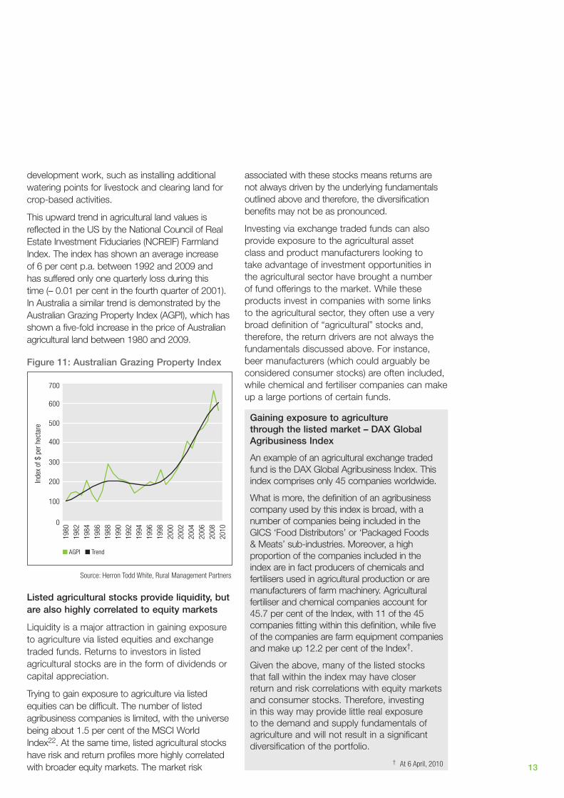
This upward trend in agricultural land values is reflected in the US by the National Council of Real Estate Investment Fiduciaries (NCREIF) Farmland Index. The index has shown an average increase of 6 per cent p.a. between 1992 and 2009 and has suffered only one quarterly loss during this time (– 0.01 per cent in the fourth quarter of 2001). In Australia a similar trend is demonstrated by the Australian Grazing Property Index (AGPI), which has shown a five-fold increase in the price of Australian agricultural land between 1980 and 2009.
Figure 11: Australian Grazing Property Index
700
Inde
x of
$ p
er h
ecta
re
600
500
400
300
100
0
200
1980
1982
1984
1986
1988
1990
1992
1994
1996
1998
2000
2002
2004
2006
2008
2010
■ AGPI ■ Trend
Source: Herron Todd White, Rural Management Partners
Listed agricultural stocks provide liquidity, but are also highly correlated to equity markets
Liquidity is a major attraction in gaining exposure to agriculture via listed equities and exchange traded funds. Returns to investors in listed agricultural stocks are in the form of dividends or capital appreciation.
Trying to gain exposure to agriculture via listed equities can be difficult. The number of listed agribusiness companies is limited, with the universe being about 1.5 per cent of the MSCI World Index22. At the same time, listed agricultural stocks have risk and return profiles more highly correlated with broader equity markets. The market risk

14
Futures only provide exposure to movements in price
Commodity futures provide an alternative to gain exposure to individual soft commodities, a strategy useful for gaining short-term exposure to spot prices. Futures are liquid investments exposed to short term volatility in prices, which are not only influenced by long term fundamentals, but also by a number of short term factors, such as supply forecasts and speculation.
Agricultural commodity prices tend to be cyclical, with long term factors influencing the trend in prices rather than impacting the short term movements. Therefore, as futures are only exposed to movements in prices, their short term and speculative nature means it is possible for an investor to make losses in the short term regardless of the long term expectations and the exposure to the longer-term agriculture theme is limited.
Futures differ to direct investment in agricultural assets, as with a direct investment returns are dependent on production, as well as price. In times where prices decrease the asset can still generate returns as it should produce a crop. However, with futures, if prices move against the investor they will make a loss on that investment.
Understanding and managing the risks to improve returnsAgricultural investments, like any other, are subject to a number of risks. In agriculture the risks include drought, pests, disease, desertification, fire, commodity price volatility and political risks. The majority of these risks can be mitigated through a thorough understanding of the investment, as well as careful due diligence and high quality management practices.
Diversification and asset selection
A portfolio of properties is far less risky than a single property, particularly if the properties are diversified across different climatic zones and commodities. Selecting and acquiring a well diversified portfolio of assets can mitigate the risks faced when investing in agriculture.
Geographic diversification reduces the impact of environmental factors that are impossible to
control, such as droughts and flooding, as well as the impact of pests and diseases. Geographic diversification reduces the likelihood that all farming operations will be adversely affected by extreme weather conditions at the same time. Diversifying across assets which produce different commodities reduces the reliance on any particular commodity, limiting the impact of negative price movements for that particular commodity.
Purchasing properties which show strong historical performance and that are located in well known production regions helps reduce production risk, as well as reducing the risk of declining land values. Experienced managers and proper due diligence procedures assist in ensuring such properties are acquired.
Management teams
Employing an experienced and high quality farm management team helps to mitigate a number of the risks outlined above. Further, these teams can drive operational efficiencies which can also improve returns.
Through the adoption of various technologies and management techniques, farm managers can reduce the risks associated with pests and disease, improve productivity and ensure suitable assets are acquired.
In recent times livestock diseases, such as Bovine spongiform encephalopathy (BSE) or ‘mad cow’ disease, have hit the headlines. These diseases often result from, or are spread through, poor conditions or deficient animal husbandry practices. Similarly, crops are at risk of plagues and diseases. These can cause damage to crops or, in worst case scenarios, result in total destruction.
Effective management can reduce these risks in a number of ways. Measures for managing animal infections include maintaining environmental conditions, maintaining checks on incumbent or recently purchased animals, and limiting herd or flock sizes. Vaccinations for some diseases and parasites and strict management of vaccination within flocks or herd can help to avoid the incidence of various diseases. For crops, the risk of pests and diseases can not always be eradicated completely, but the risk can be mitigated through the appropriate use of integrated pest and crop controls.
Making returns from agriculture

15
Obtaining economies of scale
The agriculture sector is generally characterised by small owner–operators who are unable to achieve economies of scale. Obtaining economies of scale provides a number of opportunities which are generally not presented to the small owner-operator. These opportunities assist in improving returns and managing a number of risks.
It has been shown that achieving scale can reduce the volatility of farming returns. Scale provides the ability to acquire a portfolio of land diversified across regions and capable of producing a variety of crops. Other benefits achieved through scale include:
A reduction in unit costs of production; ■
The ability to invest in technology and genetics ■
to enhance on-farm efficiencies;
Acquisition and operation of multiple, ■
geographically diversified properties;
Investment in a highly experienced ■
management team; and
Access to capital for continued growth. ■
In an Australian context, this has been witnessed in the cattle industry, with larger properties generating higher returns than their smaller counterparts.
Figure 13: Specialist beef producer performance
Farm
cas
h In
com
e/Fa
rm E
quity
Farm Size – Number of Cattle
0.0%
1.00%
2.00%
3.00%
4.00%
<300 300-600 600-1,200 1,200+
Source: ABARE Economics
Improving returns through precision agriculture
Precision agriculture involves matching agronomy with paddock variability and has come about due to the development of GPS technology which allows any position in a paddock to be regularly monitored. This allows farmers to measure variability in soil composition and crop yields. The information can then be used to make adjustments to fertiliser and chemical programs, reducing wastage which would otherwise occur if average rates were applied over the entire production area.
These techniques may require a significant initial financial outlay but, in the long run, should result in both economic and environmental improvements.
Precision agriculture has been shown to result in significant improvements in Brazil, with research on a specific farm showing positive results. The results show that, following the adoption of precision agriculture, yields have
increased by more than 20 per cent on average and operating costs have been reduced by approximately 30 per cent.
Figure 12: Improvements from precision agriculture
600
Pre Precision Ag Post Precision Ag
■ Variable cost ■ Fixed cost ■ Average yield
500
400
300
200
100
Cost
s (B
RL/H
a)
Yiel
d (B
ags/
Ha)
60
50
40
30
20
10
Source: Unigeo Precision Agriculture

16
The price rises in agricultural commodities which occurred through 2007 and 2008 brought attention to the market dynamics and the drivers of demand and supply for these commodities. It is becoming more apparent that the ability of supply growth to keep pace with the growing demand for agricultural commodities is diminishing and the result so far has been a shift in prices. Prices of many agricultural commodities are currently above historical levels and, if the gap between demand and supply continues to grow, further upward pressure will be placed on prices.
Conclusion
1 FAO Newsroom, 13 September 2006, “FAO Director-General appeals for second Green Revolution”, www.fao.org/newsroom/en/news/2006/1000392/index.html 2 USDA Foreign Agricultural Service, April 2010, “Production, Supply and Distribution Online” www.fas.usda.gov/psdonline/psdQuery.aspx 3 USDA Foreign Agricultural Service, March 2005, “Regional Analysis: Pacific Rim Population Growth Offers Export Opportunities”4 International Monetary Fund, October 2009, World Economic Outlook Database5 Population Division of the Department of Economic and Social Affairs of the United Nations Secretariat, “World Urbanization Prospects: The 2009 Revision”6 USDA Foreign Agricultural Service, April 2010, “Production, Supply and Distribution Online” www.fas.usda.gov/psdonline/psdQuery.aspx 7 Macquarie Bank Limited, Agricultural & Energy Commodities Brief, April 2009, “Soybeans: Will China's import demand continue to grow?”8 Ibid9 DB Climate Change Advisers, June 2009, “Investing in Agriculture: Far Reaching Challenge, Significant Opportunity (An Asset Management Perspective)”10 FAO Newsroom, 29 May 2008, “Agricultural commodity prices expected to remain high”, www.fao.org/newsroom/en/news/2008/1000849/index.html11 Organisation for Economic Co-Operation and Development & Food and Agriculture Organization of the United Nations, “Agricultural Outlook 2009-2018” 12 Ibid13 United Nations Environment Programme, February 2002, “Global Environment Outlook 3”, Chapter 2: State of the Environment and Policy Retrospective:
1972-2002 – Land14 Supra, Note 615 United Nations Environment Programme, October 2007, “Global Environment Outlook 4”, Chapter 4: Water 16 Ibid17 Conway, G., 1997, “The Doubly Green Revolution: Food for All in the Twenty-First Century”, Ithaca, NY, Comstock; May, R., 2000, “Melding Heart & Head”,
United Nations Environment Programme, www.unep.org/OurPlanet/imgversn/111/may.html 18 MacKenzie, D., 11 June 2008, “What Price More Food?”, New Scientist 19 World Federation of Exchanges, in Economist Blog, 29 October 2009, “Global stock market capitalisation sets new record”,
www.economistblog.com/2007/10/29/global-stock-market-capitalization-sets-new-record/20 Steward, M., 30 June 2009, “Seed capital”, Investment & Pensions Europe Magazine, www.ipe.com/articles/print.php?id=3210421 Organisation for Economic Co-Operation and Development – Directorate for Employment, Labour and Social Affairs, 2009, “Pensions at a Glance 2009:
Retirement-Income Systems in OECD Countries”, www.oecd.org/els/social/pensions/PAG , Australia: Highlights from OECD Pensions at a Glance 22 Supra, Note 18
Footnotes

18