Parton distribution functions PDFs

YETI06

A.M.Cooper-Sarkar

Oxford

1. What are they?

2. How do we determine them?

3. What are the uncertainties -experimental

-model

-theoretical (see also Thorne’s talk)

4. Why are they important?

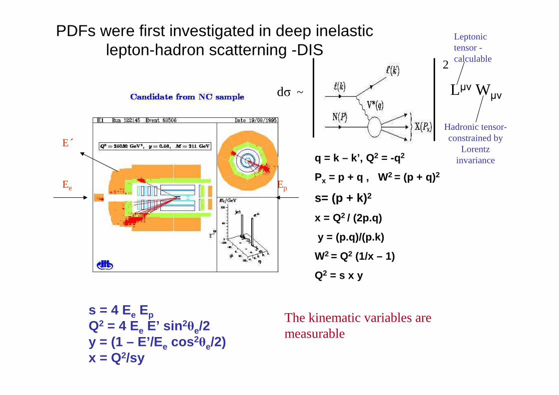
dσ ~

2

Lµν Wµν

Ee

Et

Ep

q = k – k’, Q 2 = -q2

Px = p + q , W2 = (p + q)2

s= (p + k) 2

x = Q2 / (2p.q)

y = (p.q)/(p.k)

W2 = Q2 (1/x – 1)

Q2 = s x y

s = 4 Ee EpQ2 = 4 Ee E’ sin 2θe/2y = (1 – E’/E e cos 2θe/2)x = Q2/sy

The kinematic variables are measurable

Leptonictensor -calculable

Hadronic tensor-constrained by

Lorentz invariance

PDFs were first investigated in deep inelastic lepton-hadron scatterning -DIS

d2σ(e±N) = [ Y+ F2(x,Q2) - y2 FL(x,Q2) ± Y_xF3(x,Q2)], Y± = 1 ± (1-y)2

dxdy

F2, FL and xF3 are structure functionswhich express the dependence of the cross-section

on the structure of the nucleon–The Quark-Parton model interprets these structure functions as related to the momentum distributions of quarks or partons within the nucleon AND the measurable kinematic variable x = Q2/(2p.q) is interpreted as the FRACTIONAL momentum of the incoming nucleon taken by the struck quark

(xP+q)2=x2p2+q2+2xp.q ~ 0

for massless quarks and p2~0

so

x = Q2/(2p.q)

The FRACTIONAL momentum of the incoming nucleon taken by the struck

quark is the MEASURABLE quantity x

4

22

Q

sπα

Completely generally the double differential cross-section for e-N scattering

Leptonic part hadronic part

e.g. for charged lepton beamsF2(x,Q2) = Σi ei

2(xq(x) + xq(x)) – Bjorken scalingFL(x,Q2) = 0 - spin ½ quarksxF3(x,Q2) = 0 - only γ exchange

However for neutrino beamsxF3(x,Q2)= Σi (xq(x) - xq(x)) ~ valence quark

distributions of various flavours

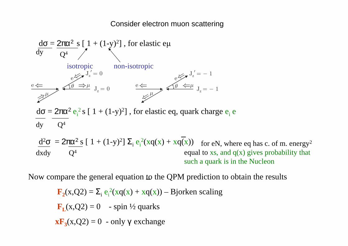
dσ = 2πα2 ei2 s [ 1 + (1-y)2] , for elastic eq, quark charge ei e

Q4dy

d2σ = 2πα2 s [ 1 + (1-y)2] Σi ei2(xq(x) + xq(x))

dxdy Q4

for eN, where eq has c. of m. energy2

equal to xs, and q(x) gives probability that such a quark is in the Nucleon

isotropic non-isotropic

Now compare the general equation to the QPM prediction to obtain the results

F2(x,Q2) = Σi ei2(xq(x) + xq(x)) – Bjorken scaling

FL(x,Q2) = 0 - spin ½ quarks

xF3(x,Q2) = 0 - only γ exchange

Consider electron muon scattering

dσ = 2πα2 s [ 1 + (1-y)2] , for elastic eµQ4dy

Compare to the general form of the cross-section for νννν/νννν scattering via W+/-

FL (x,Q2) = 0

xF3(x,Q2) = 2Σix(qi(x) - qi(x))

Valence

F2(x,Q2) = 2Σix(qi(x) + qi(x))

Valence and Sea

And there will be a relationship between F2

eN and F2νΝνΝνΝνΝ

Also NOTE ν,νν,νν,νν,ν scattering is FLAVOUR sensitive

νµµµµ-

d

uW+

W+ can only hit quarks of charge -e/3 or antiquarks -2e/3

σ(νp) ~ (d + s) + (1- y)2 (u + c)

σ(νp) ~ (u + c) (1- y)2 + (d + s)

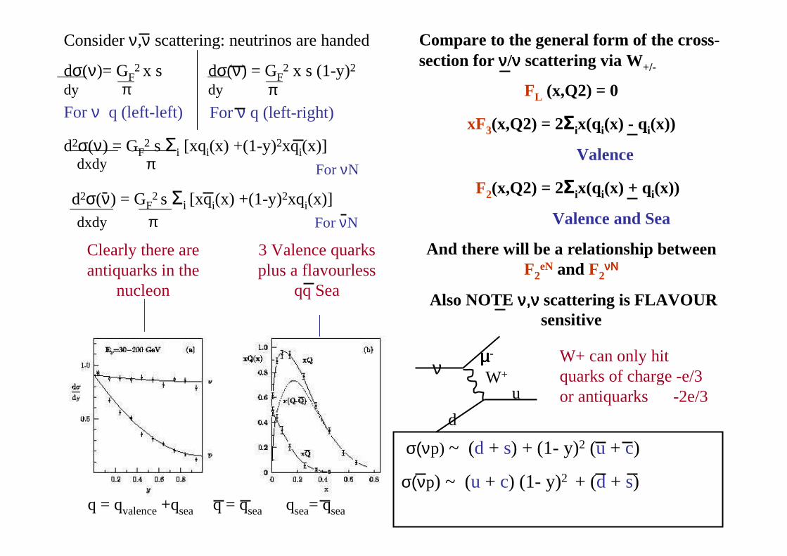
Consider ν,ν scattering: neutrinos are handed

dσ(ν)= GF2 x s dσ(ν) = GF

2 x s (1-y)2dy dyπ πFor ν q (left-left) For ν q (left-right)

d2σ(ν) = GF2 s Σi [xqi(x) +(1-y)2xqi(x)]

dxdy π For νN

d2σ(ν) = GF2 s Σi [xqi(x) +(1-y)2xqi(x)]

dxdy π For νN

Clearly there are antiquarks in the

nucleon

3 Valence quarks plus a flavourless

qq Sea

q = qvalence+qsea q = qsea qsea= qsea

)(9

4)(

9

1)(

9

1)(

9

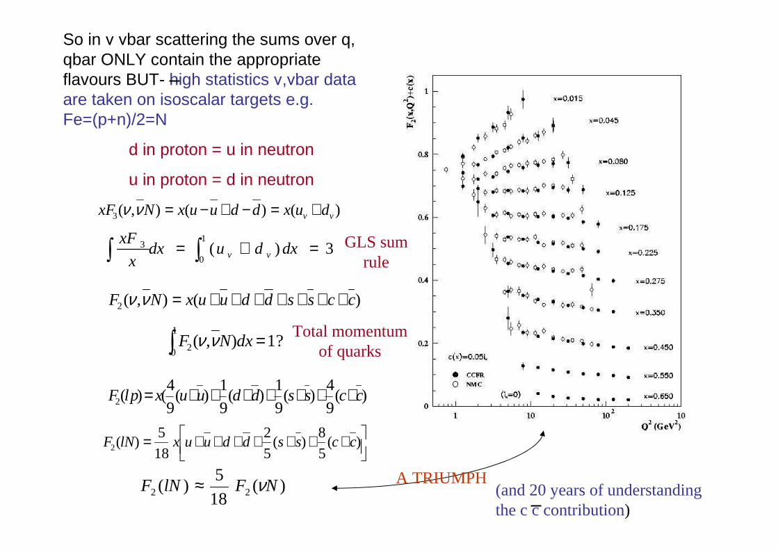
4()(2 ccssdduuxplF +++++++=

)()(),(3 vv duxdduuxNxF +=−+−=νν

So in ν νbar scattering the sums over q, qbar ONLY contain the appropriate flavours BUT- high statistics ν,νbar data are taken on isoscalar targets e.g. Fe=(p+n)/2=N

d in proton = u in neutron

u in proton = d in neutron

A TRIUMPH(and 20 years of understanding the c c contribution)

3)(1

0

3 =+= ∫∫ dxdudxx

xFvv

)(),(2 ccssdduuxNF +++++++=νν

∫ =1

0 2 ?1),( dxNF νν

+++++++= )(5

8)(

5

2

18

5)(2 ccssdduuxlNF

)(18

5)( 22 NFlNF ν≈

GLS sum rule

Total momentum of quarks

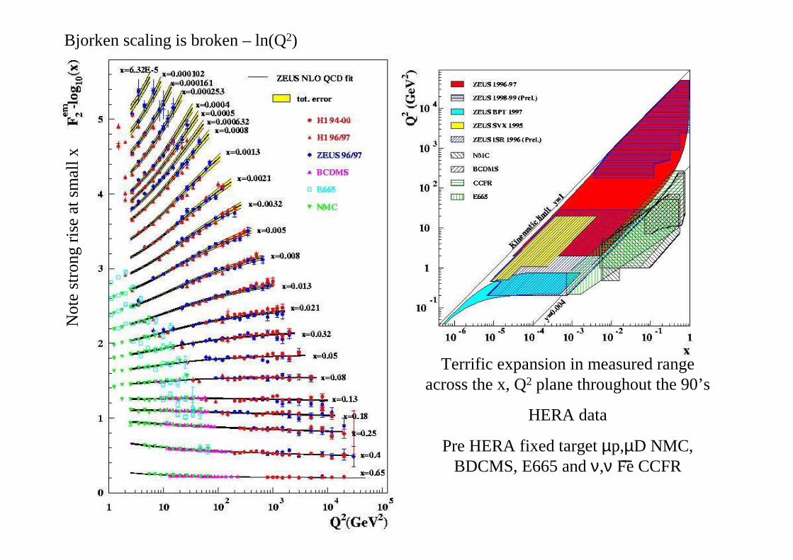
Terrific expansion in measured range across the x, Q2 plane throughout the 90’s

HERA data

Pre HERA fixed target µp,µD NMC, BDCMS, E665 and ν,ν Fe CCFR

Bjorken scaling is broken – ln(Q2)

Not

e s

tron

g ris

e a

t sm

all

x

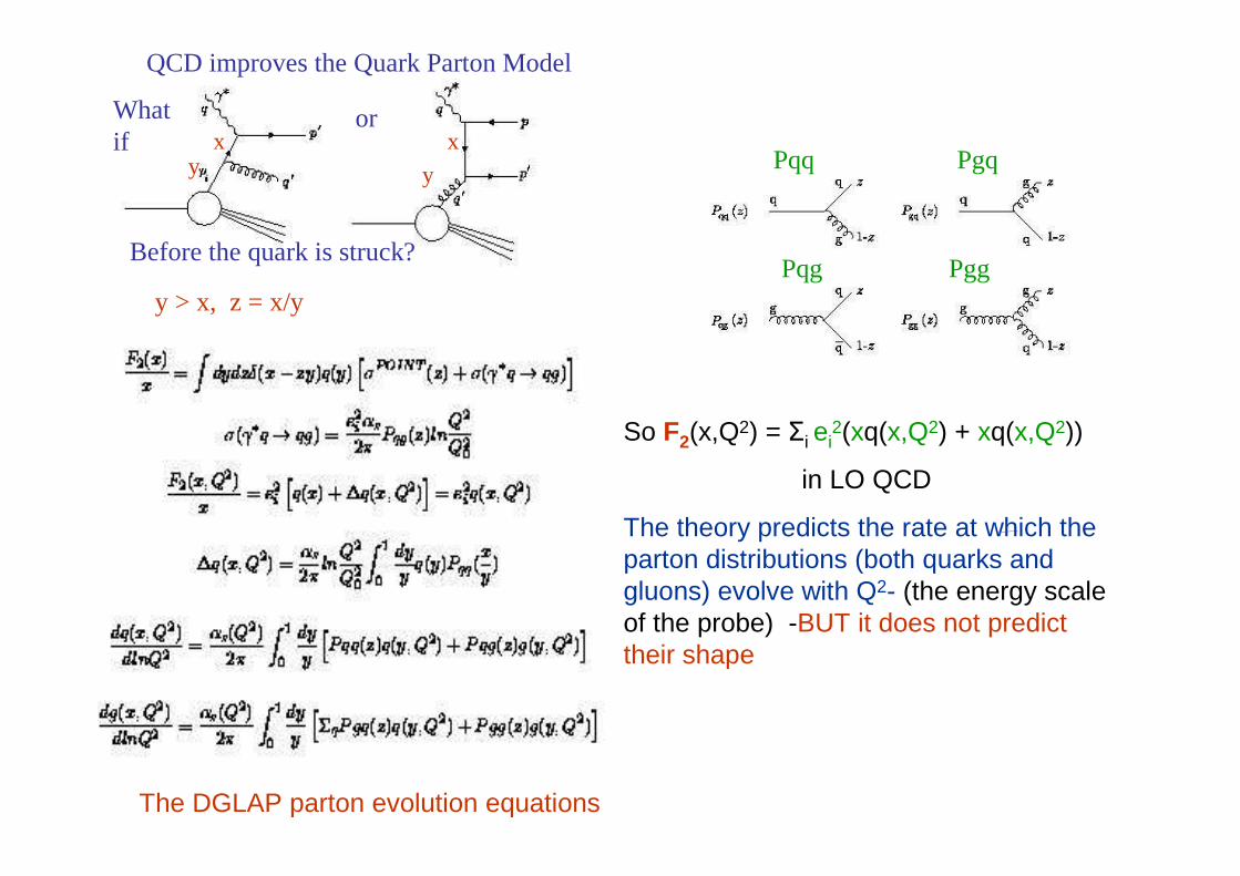
QCD improves the Quark Parton Model

What if

or

Before the quark is struck?

Pqq Pgq

Pqg Pgg

The DGLAP parton evolution equations

x xy y

y > x, z = x/y

So F2(x,Q2) = Σi ei2(xq(x,Q2) + xq(x,Q2))

in LO QCD

The theory predicts the rate at which the parton distributions (both quarks and gluons) evolve with Q2- (the energy scale of the probe) -BUT it does not predict their shape

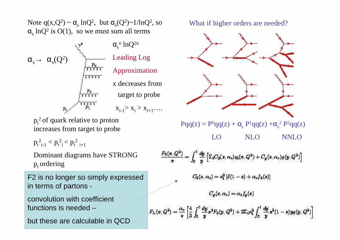
What if higher orders are needed?

Pqq(z) = P0qq(z) + αs P1qq(z) +αs2 P2qq(z)

LO NLO NNLO

Note q(x,Q2) ~ αs lnQ2, but αs(Q2)~1/lnQ2, so

αs lnQ2 is O(1), so we must sum all terms

αsn lnQ2n

Leading Log

Approximation

x decreases from

αs→ αs(Q2)

target to probe

xi-1> xi > xi+1….

pt2 of quark relative to proton

increases from target to probe

pt2i-1 < pt

2i < pt

2i+1

Dominant diagrams have STRONG pt ordering

F2 is no longer so simply expressed in terms of partons -

convolution with coefficient functions is needed –

but these are calculable in QCD

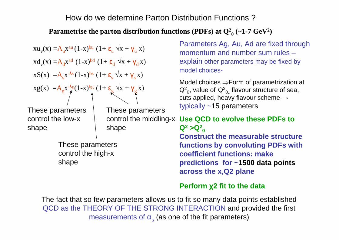
xuv(x) =Auxau(1-x)bu (1+ εu √x + γu x)

xdv(x) =Adxad (1-x)bd (1+ εd √x + γd x)

xS(x) =Asx-λs (1-x)bs (1+ εs √x + γsx)

xg(x) =Agx-λg(1-x)bg (1+ εg √x + γg x)

The fact that so few parameters allows us to fit so many data points established QCD as the THEORY OF THE STRONG INTERACTION and provided the first

measurements of αs (as one of the fit parameters)

These parameters control the low-x shape

Parameters Ag, Au, Ad are fixed through momentum and number sum rules –explain other parameters may be fixed by model choices-

Model choices ⇒Form of parametrization at Q2

0, value of Q20,, flavour structure of sea,

cuts applied, heavy flavour scheme →typically ~15 parameters

Use QCD to evolve these PDFs to Q2 >Q2

0Construct the measurable structure functions by convoluting PDFs with coefficient functions: make predictions for ~ 1500 data pointsacross the x,Q2 plane

Perform χ2 fit to the data

These parameters control the high-x shape

These parameters control the middling-x shape

How do we determine Parton Distribution Functions ?

Parametrise the parton distribution functions (PDFs) at Q20 (~1-7 GeV2)

Assuming u in proton = d in neutron – strong-isospin

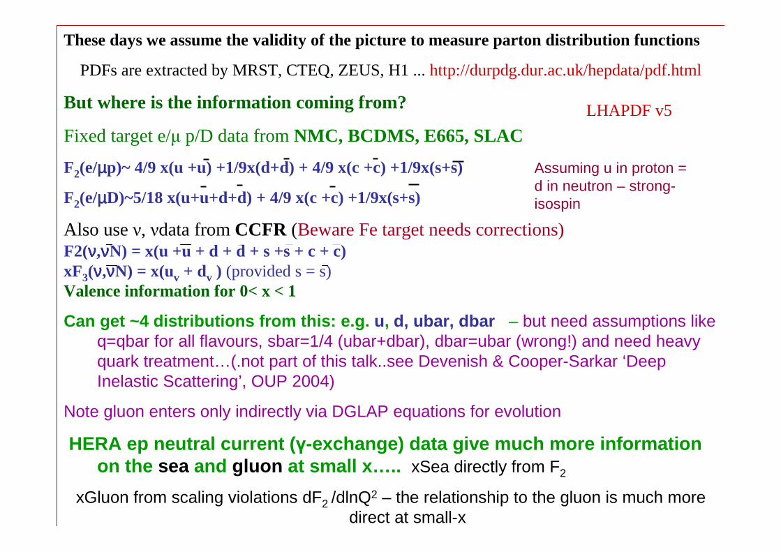
These days we assume the validity of the picture to measure parton distribution functions

PDFs are extracted by MRST, CTEQ, ZEUS, H1 ... http://durpdg.dur.ac.uk/hepdata/pdf.html

But where is the information coming from?

Fixed target e/µ p/D data from NMC, BCDMS, E665, SLAC

F2(e/µµµµp)~ 4/9 x(u +u) +1/9x(d+d) + 4/9 x(c +c) +1/9x(s+s)

F2(e/µµµµD)~5/18 x(u+u+d+d) + 4/9 x(c +c) +1/9x(s+s)

Also use ν, νdata from CCFR (Beware Fe target needs corrections)F2(νννν,ννννN) = x(u +u + d + d + s +s + c + c)xF3(νννν,ννννN) = x(uv + dv ) (provided s = s) Valence information for 0< x < 1

Can get ~4 distributions from this: e.g. u, d, ubar, dbar – but need assumptions like q=qbar for all flavours, sbar=1/4 (ubar+dbar), dbar=ubar (wrong!) and need heavy quark treatment…(.not part of this talk..see Devenish & Cooper-Sarkar ‘Deep Inelastic Scattering’, OUP 2004)

Note gluon enters only indirectly via DGLAP equations for evolution

HERA ep neutral current ( γ-exchange) data give much more information on the sea and gluon at small x….. xSea directly from F2

xGluon from scaling violations dF2 /dlnQ2 – the relationship to the gluon is much more direct at small-x

LHAPDF v5

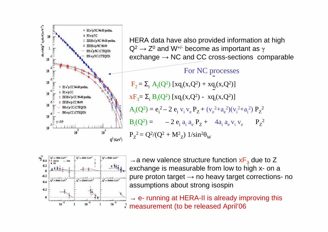
HERA data have also provided information at high Q2 → Z0 and W+/- become as important as γexchange → NC and CC cross-sections comparable

For NC processes

F2 = Σi A i(Q2) [xqi(x,Q2) + xqi(x,Q2)]

xF3= Σi Bi(Q2) [xqi(x,Q2) - xqi(x,Q2)]

A i(Q2) = ei

2 – 2 ei vi vePZ + (ve2+ae

2)(vi2+ai

2) PZ2

Bi(Q2) = – 2 ei ai ae PZ + 4ai aevi ve PZ

2

PZ2 = Q2/(Q2 + M2

Z) 1/sin2θW

→a new valence structure function xF3 due to Z exchange is measurable from low to high x- on a pure proton target → no heavy target corrections- no assumptions about strong isospin

→ e- running at HERA-II is already improving this measurement (to be released April’06

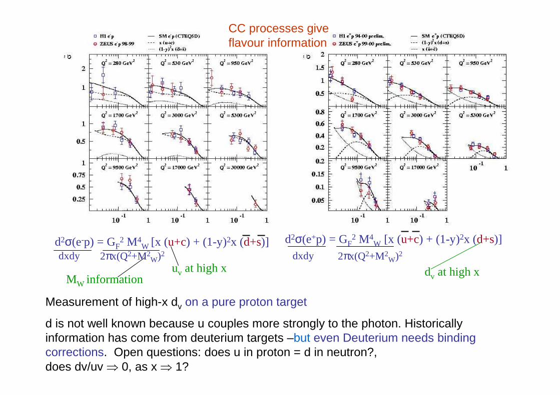
CC processes give flavour information

d2σ(e-p) = GF2 M4

W [x (u+c) + (1-y)2x (d+s)] dxdy 2πx(Q2+M2

W)2

d2σ(e+p) = GF2 M4

W [x (u+c) + (1-y)2x (d+s)]dxdy 2πx(Q2+M2

W)2

MW informationuv at high x dv at high x

Measurement of high-x dv on a pure proton target

d is not well known because u couples more strongly to the photon. Historically information has come from deuterium targets –but even Deuterium needs binding corrections. Open questions: does u in proton = d in neutron?, does dv/uv ⇒ 0, as x ⇒ 1?

ZEUS

0

0.1

0.2

0.3

0.4

0.5

0.6

0.7

0.8

10-3

10-2

10-1

1

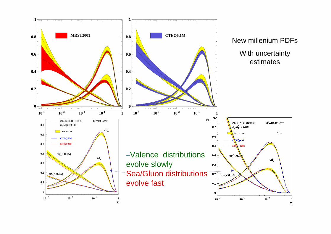
ZEUS NLO QCD fit

αs(MZ2) = 0.118

tot. error

CTEQ 6M

MRST2001

Q2=10 GeV2

xuv

xdv

xg(× 0.05)

xS(× 0.05)

x

xf

10 10 10 10 1 10 10 10 10 1

0

0.2

0.4

0.6

0.8

1

-410 -310 -210 -110 1

0

0.2

0.4

0.6

0.8

1

MRST2001

0

0.2

0.4

0.6

0.8

1

-410 -310 -210 -110 1

0

0.2

0.4

0.6

0.8

1

CTEQ6.1M

0

0.2

0.4

0.6

0.8

1

x

–Valence distributions evolve slowly Sea/Gluon distributions evolve fast

New millenium PDFs

With uncertainty estimates

So how certain are we? First, some quantitative measure of the progress made over 20 years of PDF fitting ( thanks to Wu-ki Tung)

22642361205301378MRST01/2

20291231595081239CTQ6M 02

23962271116591398MRS98 ~’98

25132062276661414CTQ4M ~’98

579121330237791497GRV94 ~’94

30542312499831590MRSA ~’94

364222464612411531CTQ2M ~’94

1038128057777091815KMRS ~‘90

833321885737073551MoTu ~‘90

15187275159950058308DuOw ‘84

219293312373775011475EHLQ ‘84

18221231454841070# Expt pts.

TotalJetsDY-WHERAFixed-tgt

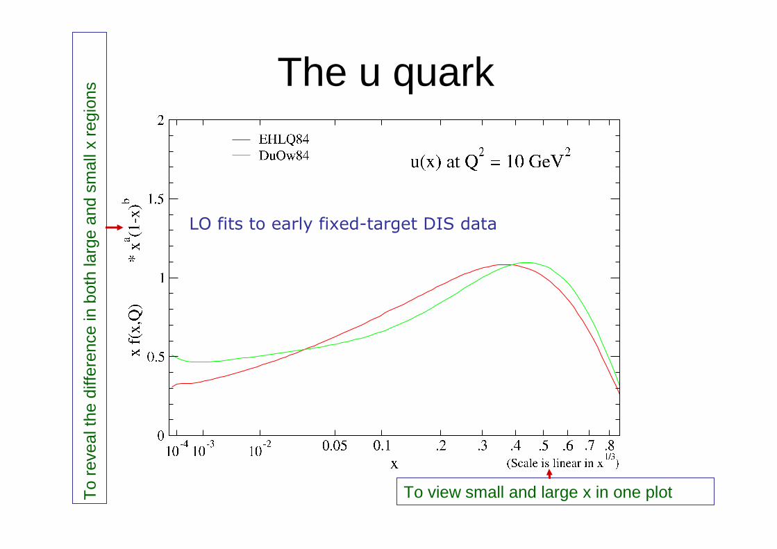
The u quark

LO fits to early fixed-target DIS data

To view small and large x in one plotTo

reve

al th

e di

ffere

nce

in b

oth

larg

e an

d sm

all x

reg

ions

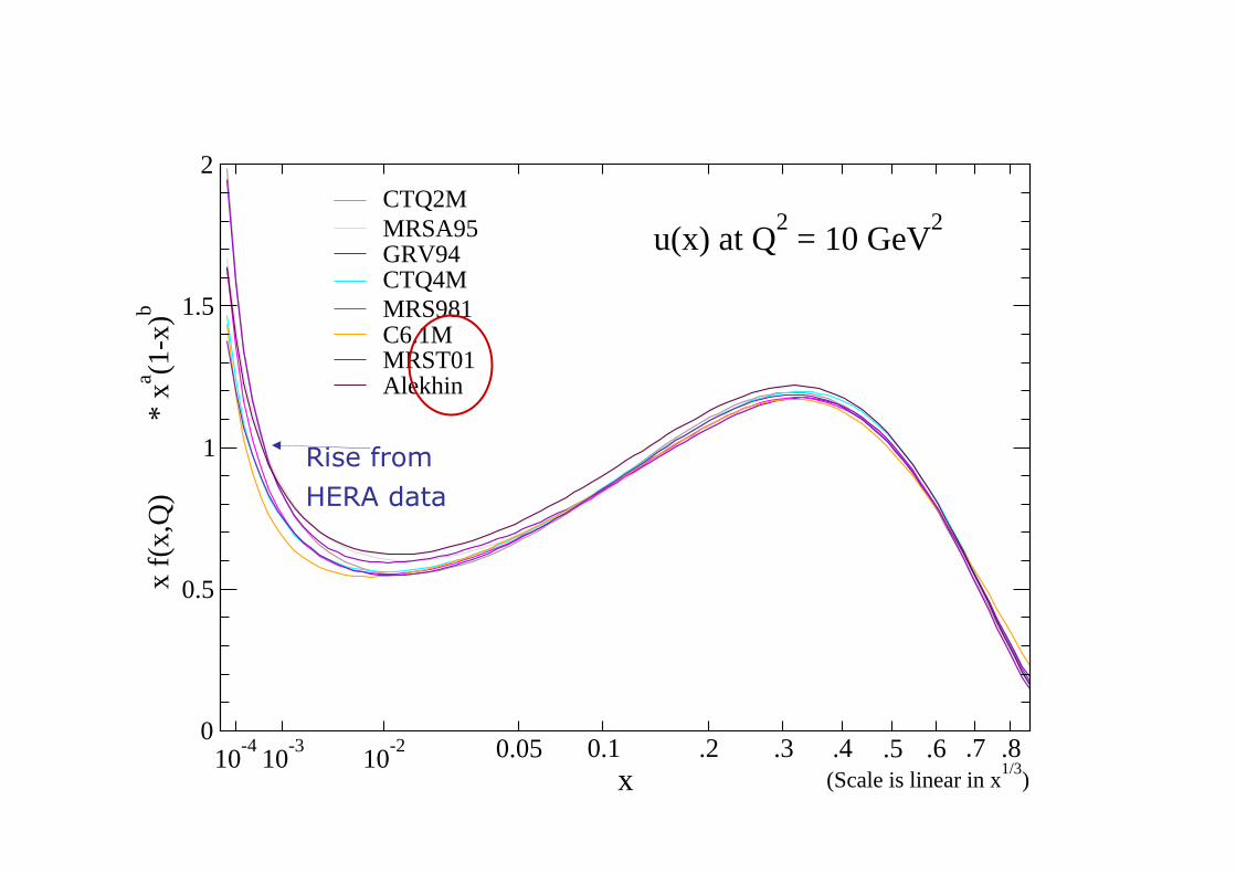
10-4

10-3

10-2 0.05 0.1 .2 .3 .4 .5 .6 .7 .8

x

0

0.5

1

1.5

2x

f(x,

Q)

*

xa (1-x

)b

CTQ2MMRSA95GRV94CTQ4MMRS981C6.1MMRST01Alekhin

(Scale is linear in x1/3

)

u(x) at Q2 = 10 GeV

2

Rise from

HERA data

10-4

10-3

10-2 0.05 0.1 .2 .3 .4 .5 .6 .7 .8

x

0

0.5

1

f(x,

Q)

*

xa (1-x

)b

EHLQ84DuOw84MoTu90KMRS90CTQ2MMRSA95GRV94CTQ4MMRS981C6.1MMRST01Alekhin

(Scale is linear in x1/3

)

D quark at Q2 = 10 GeV

2

The old and the new

d quark

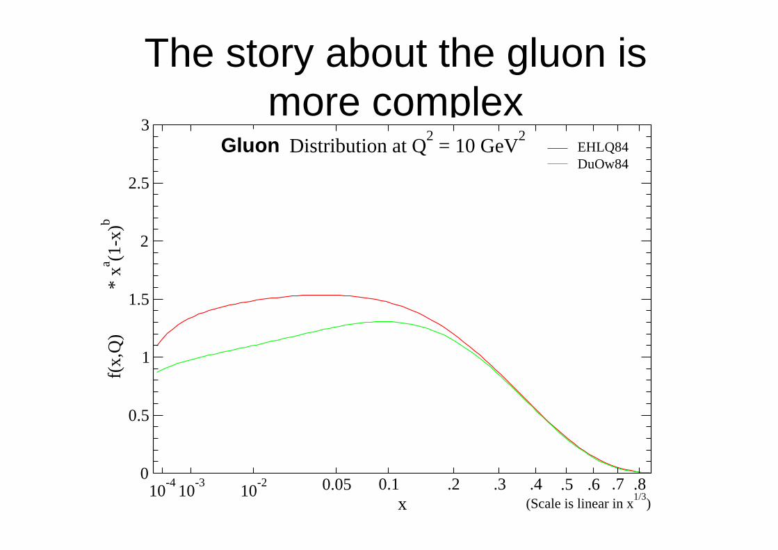
The story about the gluon is more complex

10-4

10-3

10-2 0.05 0.1 .2 .3 .4 .5 .6 .7 .8

x

0

0.5

1

1.5

2

2.5

3f(

x,Q

)

* xa (1

-x)b

EHLQ84DuOw84

(Scale is linear in x1/3

)

Gloun Distribution at Q2 = 10 GeV

2Gluon

Gluon

HERA

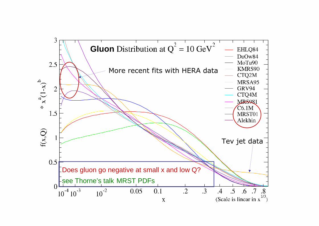
Gluon

Does gluon go negative at small x and low Q?

see Thorne’s talk MRST PDFs

More recent fits with HERA data

Tev jet data

ZEUS

1

10

10 2

10 3

10 4

10 5

10-4

10-3

10-2

10-1

1

<2%<4%<10%>10%

y=1

y=10-1

y=10-2

y=10-3

Kinematic limit

θe=177o

E' e=8 GeV

W=20GeV

x

Q2 (

GeV

2 )Statistical Uncertainty

1

10

10 2

10 3

10 4

10 5

10-4

10-3

10-2

10-1

1

<2%<4%<10%>10%

y=1

y=10-1

y=10-2

y=10-3

Kinematic limit

θe=177o

E' e=8 GeV

W=20GeV

x

Q2 (

GeV

2 )

Systematic Uncertainty

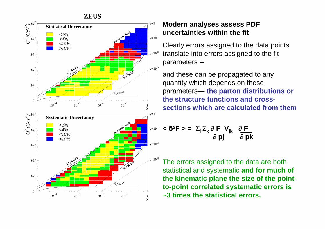
Modern analyses assess PDF uncertainties within the fit

Clearly errors assigned to the data points translate into errors assigned to the fit parameters --

and these can be propagated to any quantity which depends on these parameters— the parton distributions or the structure functions and cross-sections which are calculated from them

< б2F > = Σj Σk ∂ F Vjk ∂ F∂ pj ∂ pk

The errors assigned to the data are both statistical and systematic and for much of the kinematic plane the size of the point-to-point correlated systematic errors is ~3 times the statistical errors.

0

10

20

30

10-3

10-2

10-1

0

10

20

30

10-3

10-2

10-1

0

20

40

10-3

10-2

10-1

0

20

40

10-3

10-2

10-1

-20

-10

0

10

20

10-3

10-2

10-1 -20

-10

0

10

20

10-3

10-2

10-1

-4

-2

0

2

4

10-3

10-2

10-1

-4

-2

0

2

4

1 10 102

103

ZEUSUncorrelated sys. uncertainty

y

Unc

erta

inty

(%

)

Total systematic uncertainty

yStatistical uncertainty

y

Stat.⊕ Sys. uncertainty

y

PHP ±35% { 9}

y

Cells at low Y { 10}

yRCAL energy ±2% { 7}

y

RCAL halves ±2 mm { 2}

Q2 (GeV2)

Q2<50GeV2

50<Q2<500GeV2

Q2>500GeV2

What are the sources of correlated systematic errors? Normalisations are an obvious

exampleBUT there are more subtle cases- e.g.

Calorimeter energy scale/angular resolutions can move events between x,Q2 bins and thus change the shapeof experimental distributions

Vary the estimate of the photo-production background

Vary energy scales in different regions of the calorimeter

Vary position of the RCAL halves

Why does it matter?

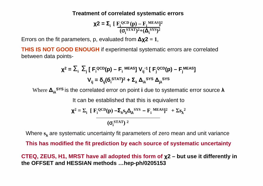
Treatment of correlated systematic errors

χ2 = Σi [ FiQCD (p) – Fi

MEAS]2

(σσσσiSTAT)2+(∆i

SYS)2

Errors on the fit parameters, p, evaluated from ∆χ2 = 1,

THIS IS NOT GOOD ENOUGH if experimental systematic errors are correlated between data points-

χ2 = Σi Σj [ F iQCD(p) – F i

MEAS] V ij-1 [ F j

QCD(p) – F jMEAS]

Vij = δij(бiSTAT)2 + Σλ ∆iλ

SYS ∆jλSYS

Where ∆iλSYS is the correlated error on point i due to systematic error source λ

It can be established that this is equivalent to

χ2 = Σi [ FiQCD(p) –Σλsλλλλ∆∆∆∆iλλλλ

SYS – FiMEAS]2 + Σsλλλλ

2

(σσσσiSTAT) 2

Where sλ are systematic uncertainty fit parameters of zero mean and unit variance

This has modified the fit prediction by each source of systematic uncertainty

CTEQ, ZEUS, H1, MRST have all adopted this form of χ2 – but use it differently in the OFFSET and HESSIAN methods …hep-ph/0205153

How do experimentalists usually proceed: OFFSET met hod

1. Perform fit without correlated errors (s λ = 0) for central fit

2. Shift measurement to upper limit of one of its sy stematic uncertainties (s λ = +1)

3. Redo fit, record differences of parameters from t hose of step 1

4. Go back to 2, shift measurement to lower limit (s λ = -1)

5. Go back to 2, repeat 2-4 for next source of syste matic uncertainty

6. Add all deviations from central fit in quadrature (positive and negative deviations added in quadrature separately)

7. This method does not assume that correlated systema tic uncertainties are Gaussian distributed

Fortunately, there are smart ways to do this (Pasca ud and Zomer LAL-95-05, Botje hep-ph-0110123)

A1

Slide 25

A1 Cooper-Sarkar, 15/03/2004

There are other ways to treat correlated systematic errors- HESSIAN method (covariance method)

Allow s λ parameters to vary for the central fit.

If we believe the theory why not let it calibrate t he detector(s)? Effectively the theoretical prediction is not fitted to the central values of published experimental data, but allows these data points to move collectively according to their correlated systematic uncertainties

The fit determines the optimal settings for correl ated systematic shifts such that the most consistent fit to all data sets is ob tained. In a global fit the systematic uncertainties of one experiment will correlate to those of another through the fit

The resulting estimate of PDF errors is much smalle r than for the Offset method for ∆χ2 = 1

We must be very confident of the theory to trust it for calibration – but more dubiously we must be very confident of the model choices we made in setting boundary conditions

We must check that superficial changes of model choice (values of Q20, form of

parametrization…) do not result in large changes of sλ

We must also check that |s λ| values are not >>1, so that data points are not shifted far outside their one standard deviation er rors - Data inconsistencies!

200

220

240

260

280

0.116 0.118 0.12 0.122

χ2 − n

o. p

ts

Total (2097 pts)

0

20

40

60

0.116 0.118 0.12 0.122

D0 jet (82 pts)

CDF1B jet (31 pts)

Total jet (113 pts)

60

80

100

120

140

0.116 0.118 0.12 0.122

χ2 − n

o. p

ts

E605 (136 pts)

0

20

40

60

80

0.116 0.118 0.12 0.122

BCDMS F2µp (167 pts)

BCDMS F2µd (155 pts)

-40

-20

0

20

40

0.116 0.118 0.12 0.122

αs(MZ2)

χ2 − n

o. p

ts

NMC F2µp (126 pts)

NMC F2µd (126 pts)

SLAC F2 ep (53 pts)

SLAC F2 ed (54 pts)

-40

-20

0

20

0.116 0.118 0.12 0.122

αs(MZ2)

CCFR F2νN (74 pts)

CCFR xF3νN (105 pts)

H1 (400 pts)

ZEUS (272 pts)

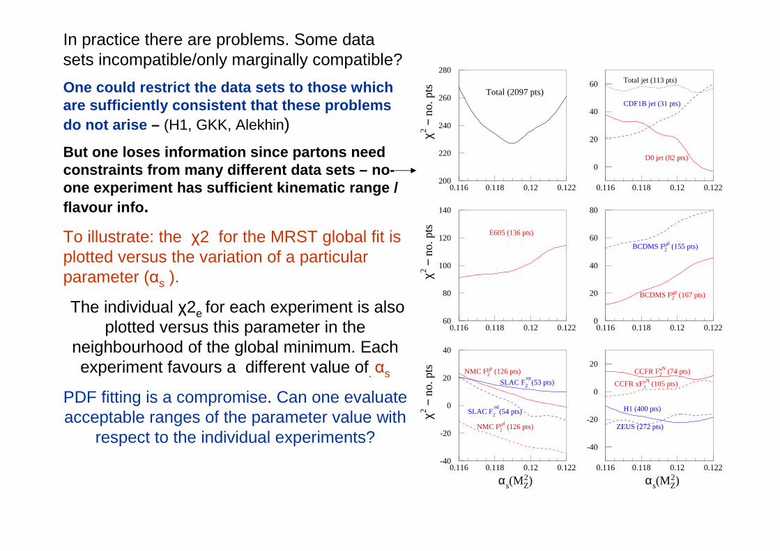
In practice there are problems. Some data sets incompatible/only marginally compatible?

One could restrict the data sets to those which are sufficiently consistent that these problems do not arise – (H1, GKK, Alekhin)

But one loses information since partons need constraints from many different data sets – no-one experiment has sufficient kinematic range / flavour info .

To illustrate: the χ2 for the MRST global fit is plotted versus the variation of a particular parameter (αs ).

The individual χ2e for each experiment is also plotted versus this parameter in the

neighbourhood of the global minimum. Each experiment favours a different value of. αs

PDF fitting is a compromise. Can one evaluate acceptable ranges of the parameter value with

respect to the individual experiments?

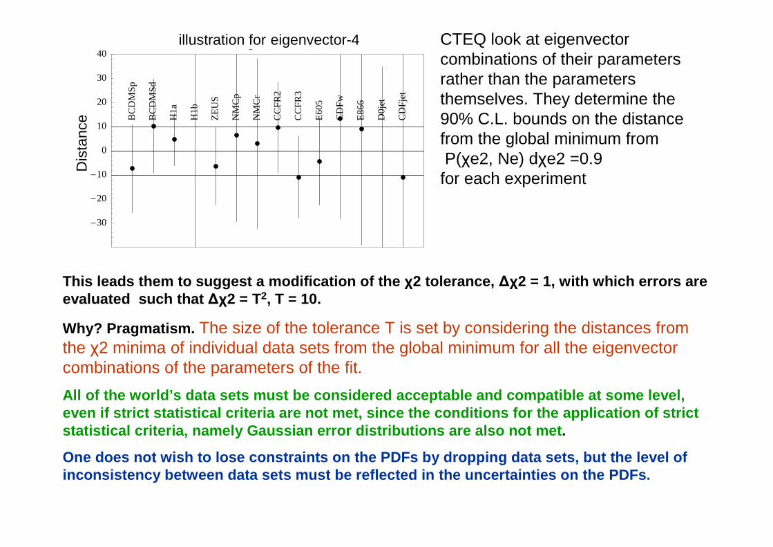
This leads them to suggest a modification of the χ2 tolerance, ∆χ2 = 1, with which errors are evaluated such that ∆χ2 = T2, T = 10.

Why? Pragmatism. The size of the tolerance T is set by considering the distances from the χ2 minima of individual data sets from the global minimum for all the eigenvector combinations of the parameters of the fit.

All of the world’s data sets must be considered acc eptable and compatible at some level, even if strict statistical criteria are not met, si nce the conditions for the application of strict statistical criteria, namely Gaussian error distrib utions are also not met .

One does not wish to lose constraints on the PDFs by dropping data sets, but the level of inconsistency between data sets must be reflected i n the uncertainties on the PDFs.

-30

-20

-10

0

10

20

30

40Eigenvector 4

BC

DM

Sp

BC

DM

Sd

H1a

H1b

ZE

US

NM

Cp

NM

Cr

CC

FR

2

CC

FR

3

E60

5

CD

Fw

E86

6

D0j

et

CD

Fje

t

CTEQ look at eigenvector combinations of their parameters rather than the parameters themselves. They determine the 90% C.L. bounds on the distance from the global minimum fromP(χe2, Ne) dχe2 =0.9

for each experiment

illustration for eigenvector-4

Dis

tanc

e

Offset method Hessian method T=1

Compare gluon PDFs for Hessian and Offset methods fo r the ZEUS fit analysis

Hessian method T=7

The Hessian method gives comparable size of error b and as the Offset method, when the tolerance is raised to T ~ 7 – (similar ball park to CTEQ, T=10)

Note this makes the error band large enough to encompass reasonable variations of model choice. (For the ZEUS global fit √2N=50, where N is the number of degrees of freedom)

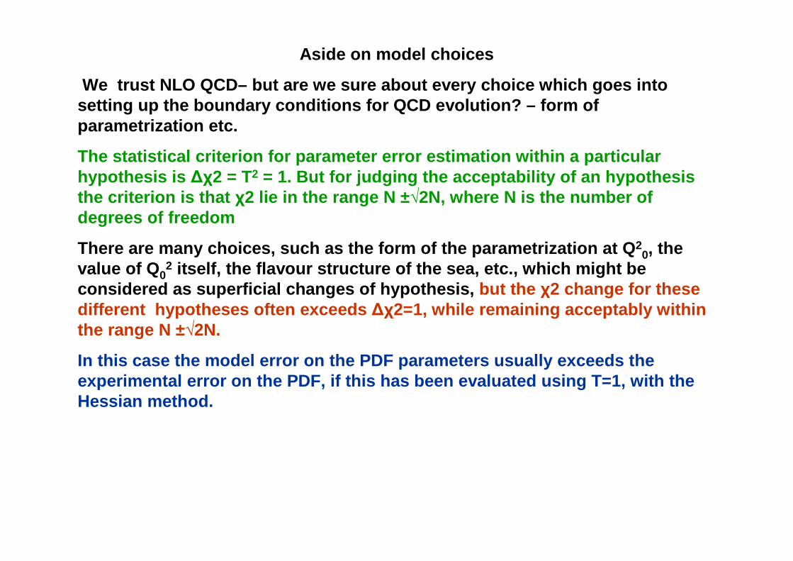
Aside on model choices

We trust NLO QCD– but are we sure about every choic e which goes into setting up the boundary conditions for QCD evolutio n? – form of parametrization etc.

The statistical criterion for parameter error estim ation within a particular hypothesis is ∆χ2 = T2 = 1. But for judging the acceptability of an hypoth esis the criterion is that χ2 lie in the range N ± √2N, where N is the number of degrees of freedom

There are many choices, such as the form of the par ametrization at Q 20, the

value of Q 02 itself, the flavour structure of the sea, etc., whic h might be

considered as superficial changes of hypothesis, but the χ2 change for these different hypotheses often exceeds ∆χ2=1, while remaining acceptably within the range N ± √2N.

In this case the model error on the PDF parameters usually exceeds the experimental error on the PDF, if this has been eva luated using T=1, with the Hessian method.

CTEQ6.1MRST2001

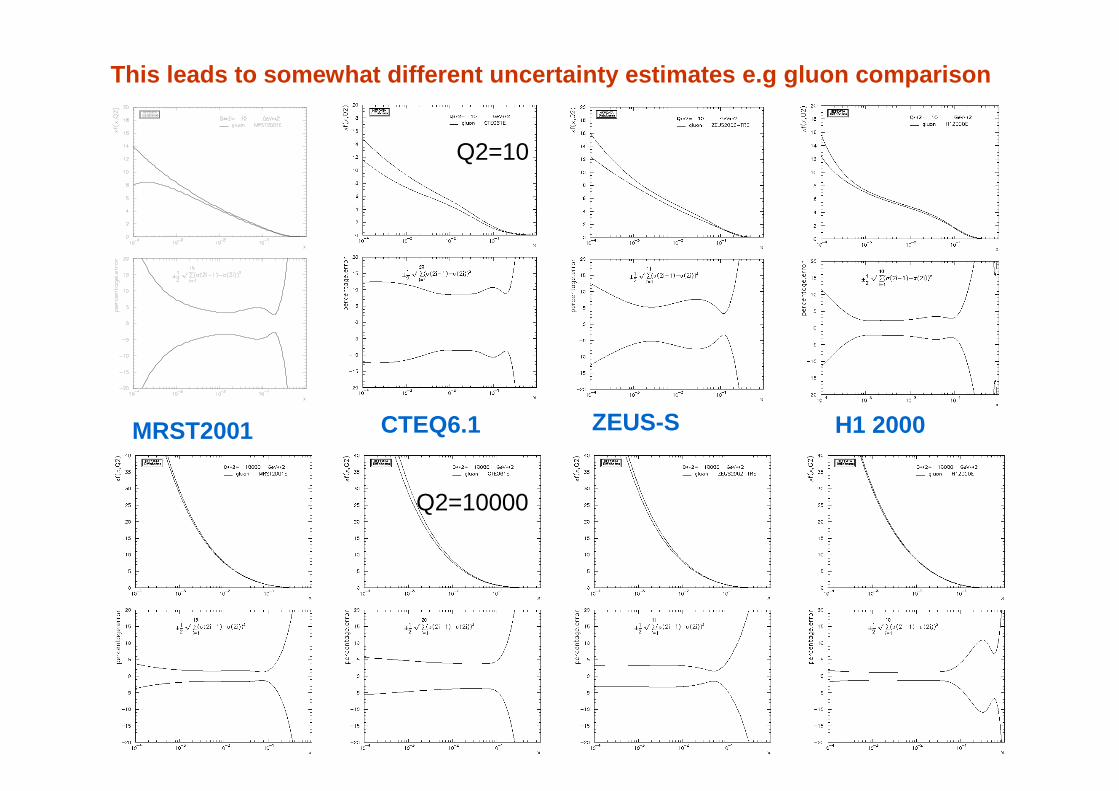
This leads to somewhat different uncertainty estima tes e.g gluon comparison

Q2=10

Q2=10000

ZEUS-S H1 2000

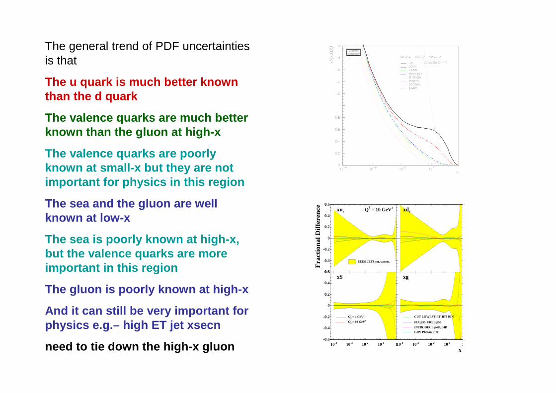
The general trend of PDF uncertainties is that

The u quark is much better known than the d quark

The valence quarks are much better known than the gluon at high-x

The valence quarks are poorly known at small-x but they are not important for physics in this region

The sea and the gluon are well known at low-x

The sea is poorly known at high-x, but the valence quarks are more important in this region

The gluon is poorly known at high-x

And it can still be very important for physics e.g.– high ET jet xsecn

need to tie down the high-x gluon

vxu 2 = 10 GeV2Q

ZEUS-JETS tot. uncert.

vxd

xS

2 = 4 GeV20 Q

2 = 10 GeV20 Q

xg

CUT LOWEST-ET JET BIN

FIX p3S, FREE p5S

INTRODUCE p4U, p4D

GRV Photon PDF

-410 -310 -210 -110 1 -410 -310 -210 -110 1-0.6

-0.4

-0.2

0

0.2

0.4

0.6-0.6

-0.4

-0.2

0

0.2

0.4

0.6

x

Fra

ctio

nal D

iffer

ence

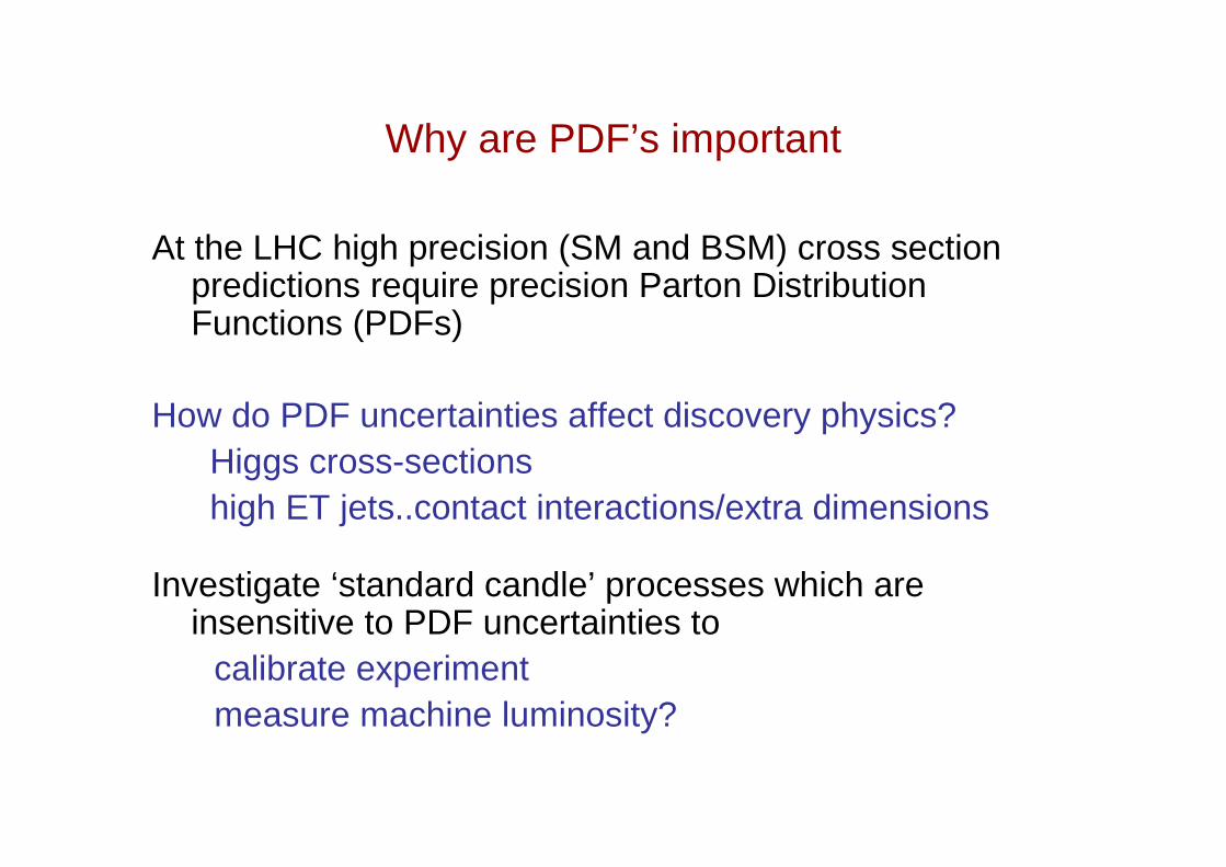
Why are PDF’s important

At the LHC high precision (SM and BSM) cross section predictions require precision Parton Distribution Functions (PDFs)

How do PDF uncertainties affect discovery physics?Higgs cross-sectionshigh ET jets..contact interactions/extra dimensions

Investigate ‘standard candle’ processes which are insensitive to PDF uncertainties to

calibrate experiment measure machine luminosity?

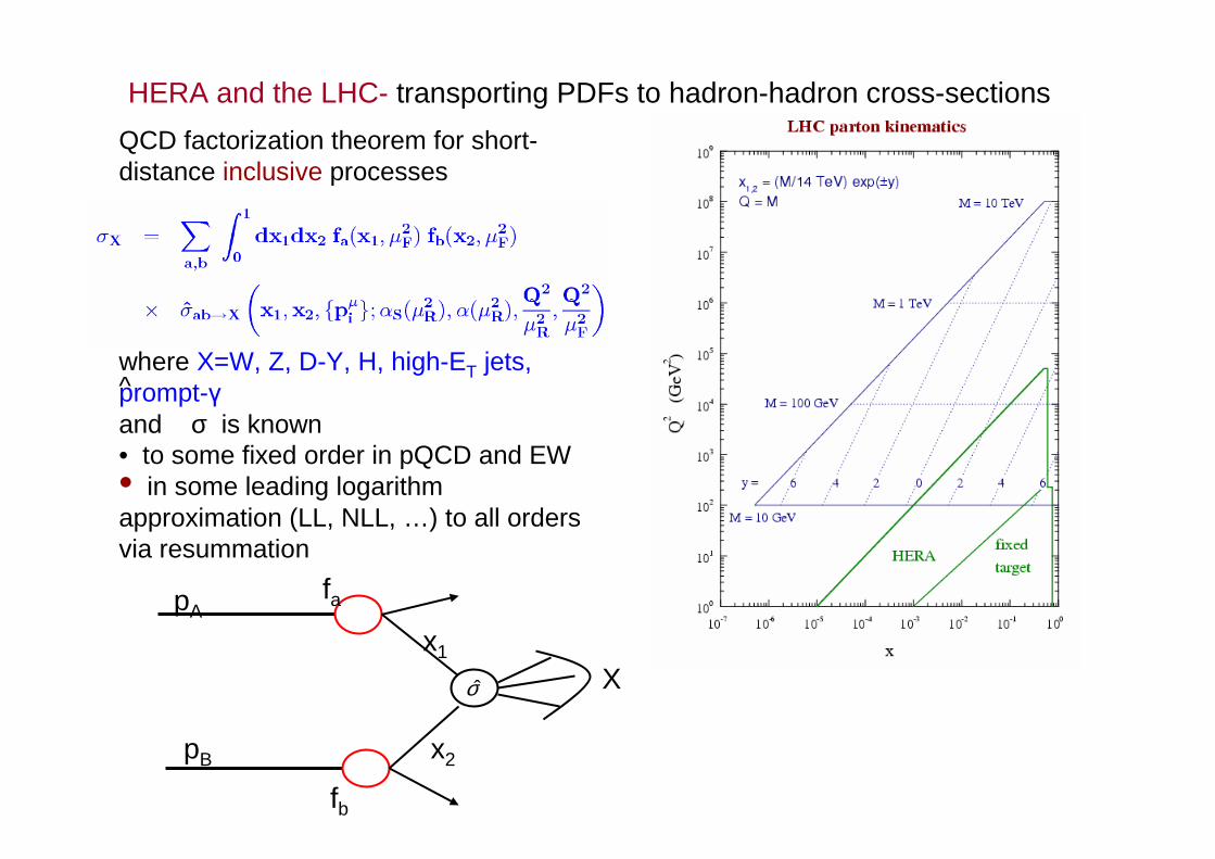
HERA and the LHC- transporting PDFs to hadron-hadron cross-sections

QCD factorization theorem for short-distance inclusive processes

where X=W, Z, D-Y, H, high-ET jets, prompt-γand σ is known • to some fixed order in pQCD and EW• in some leading logarithm approximation (LL, NLL, …) to all orders via resummation

^

pA

pB

fa

fb

x1

x2

σ̂ X

0 100 200 300 400 500-1.5

-1

-0.5

0

0.5

1

1.5

0 100 200 300 400 500-1.5

-1

-0.5

0

0.5

1

1.5

data uncertainty

(MRST2002)

(GeV)TE

(dat

a-th

eory

)/th

eory

CDF ~ 0.25η MRST ~ 0.74η

~ 1.23η ~ 1.72η

0 100 200 300 400 5000 100 200 300 400 500-1.5

-1

-0.5

0

0.5

1

1.5-1.5

-1

-0.5

0

0.5

1

1.5

(GeV)TE

(da

ta-t

he

ory

)/th

eo

ry

D0

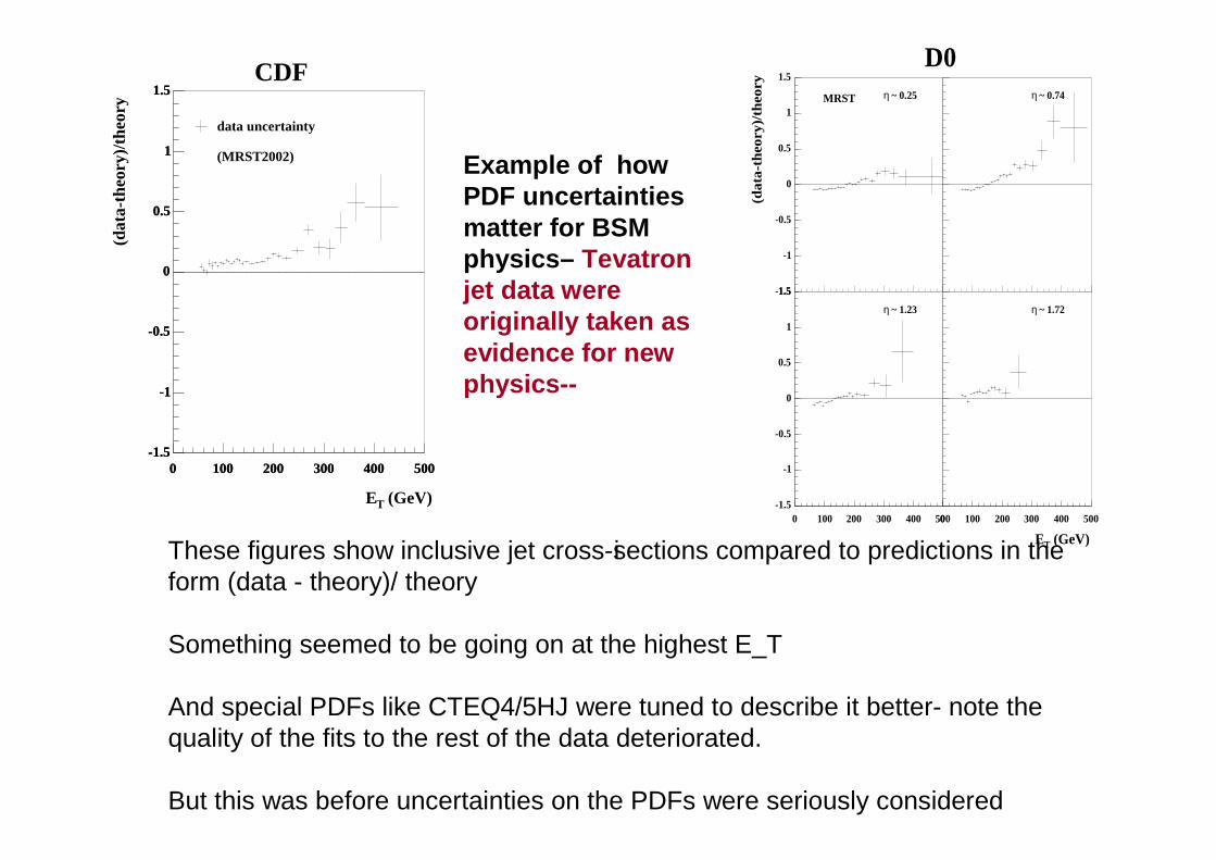
Example of how PDF uncertainties matter for BSM physics– Tevatronjet data were originally taken as evidence for new physics--

iThese figures show inclusive jet cross-sections compared to predictions in the form (data - theory)/ theory

Something seemed to be going on at the highest E_T

And special PDFs like CTEQ4/5HJ were tuned to describe it better- note the quality of the fits to the rest of the data deteriorated.

But this was before uncertainties on the PDFs were seriously considered

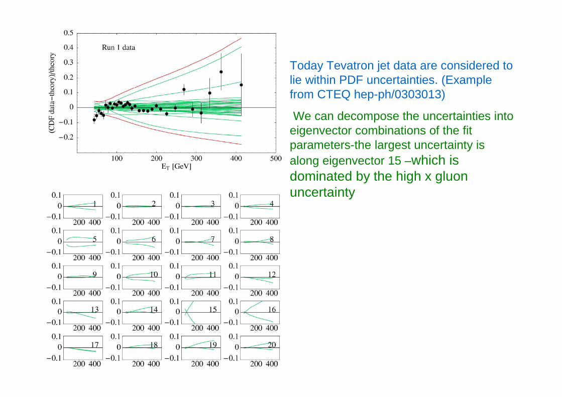
Today Tevatron jet data are considered to lie within PDF uncertainties. (Example from CTEQ hep-ph/0303013)

We can decompose the uncertainties into eigenvector combinations of the fit parameters-the largest uncertainty is along eigenvector 15 –which is dominated by the high x gluon uncertainty

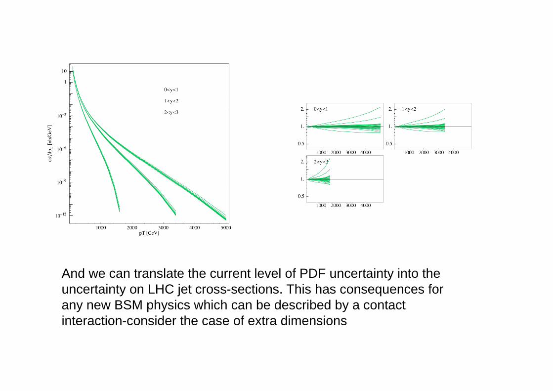
And we can translate the current level of PDF uncertainty into the uncertainty on LHC jet cross-sections. This has consequences for any new BSM physics which can be described by a contact interaction-consider the case of extra dimensions

2XD

4XD

6XD

SM

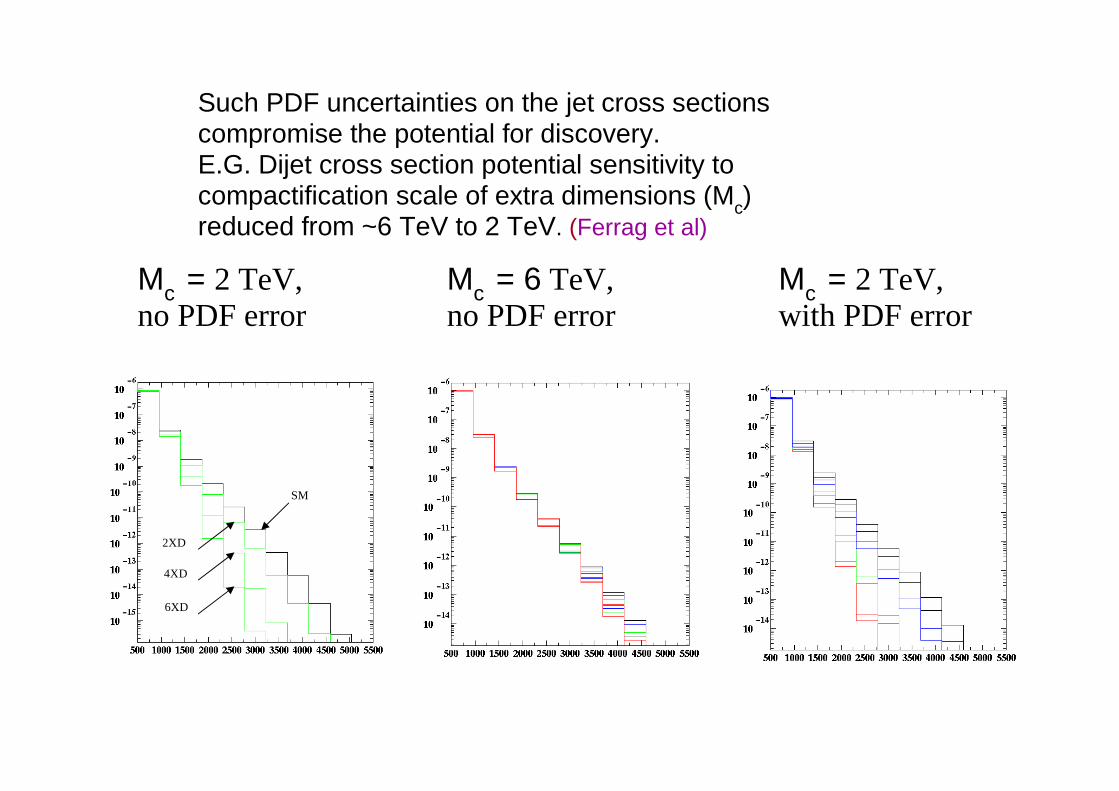
Such PDF uncertainties on the jet cross sections compromise the potential for discovery.E.G. Dijet cross section potential sensitivity to compactification scale of extra dimensions (Mc) reduced from ~6 TeV to 2 TeV. (Ferrag et al)

Mc = 2 TeV,no PDF error

Mc = 2 TeV,with PDF error

Mc = 6 TeV,no PDF error

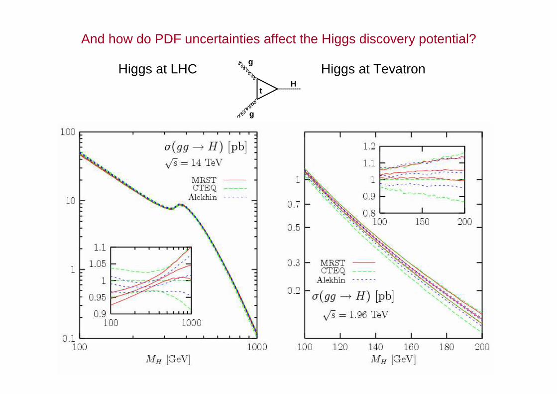
Higgs at LHC Higgs at Tevatron

And how do PDF uncertainties affect the Higgs discovery potential?

g

g

Ht

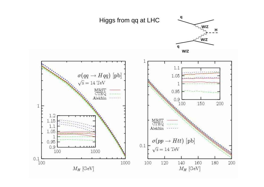
Higgs from qq at LHC

q

q

W/Z

W/Z

W/Z

H

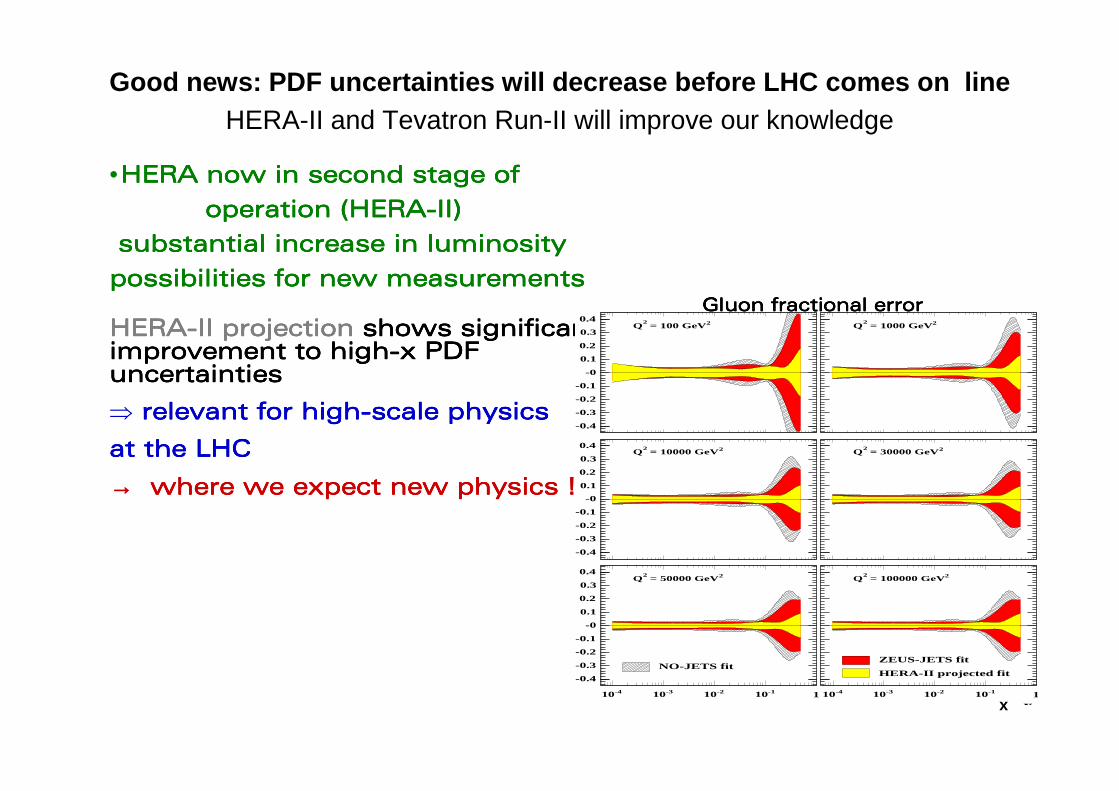
•HERA now in second stage of HERA now in second stage of HERA now in second stage of HERA now in second stage of

operation (HERAoperation (HERAoperation (HERAoperation (HERA----II)II)II)II)

substantial increase in luminositysubstantial increase in luminositysubstantial increase in luminositysubstantial increase in luminosity

possibilities for new measurementspossibilities for new measurementspossibilities for new measurementspossibilities for new measurements

HERAHERAHERAHERA----II projectionII projectionII projectionII projection shows significant shows significant shows significant shows significant improvement to highimprovement to highimprovement to highimprovement to high----x PDF x PDF x PDF x PDF uncertainties uncertainties uncertainties uncertainties

⇒ relevant for highrelevant for highrelevant for highrelevant for high----scale physics scale physics scale physics scale physics

at the LHC at the LHC at the LHC at the LHC

→→→→ where we expect new physics !!where we expect new physics !!where we expect new physics !!where we expect new physics !!

2 = 100 GeV2

Q 2 = 1000 GeV2

Q

2 = 10000 GeV2Q 2 = 30000 GeV2Q

NO-JETS fit

2 = 50000 GeV2Q

ZEUS-JETS fit

HERA-II projected fit

2 = 100000 GeV2Q

-410 -310 -210 -110 1 -410 -310 -210 -110 1

-0.4

-0.3

-0.2

-0.1

-0

0.1

0.2

0.3

0.4

-0.4

-0.3

-0.2

-0.1

-0

0.1

0.2

0.3

0.4

-0.4

-0.3

-0.2

-0.1

-0

0.1

0.2

0.3

0.4

x

gluon

fracti

onal

error

Gluon fractional errorGluon fractional errorGluon fractional errorGluon fractional error

x

Good news: PDF uncertainties will decrease before LHC comes on lineHERA-II and Tevatron Run-II will improve our knowledge

MRST PDF

NNLO corrections small ~ few%NNLO residual scale dependence < 1%

-6 -4 -2 0 2 4 60

1

2

3

4

5

x1 = 0.0003x2 = 0.12

x1 = 0.12x2 = 0.0003

x1 = 0.006x2 = 0.006

yW

MRST2002-NLO LHCdσ

W/d

y W .

Blν

(nb

)

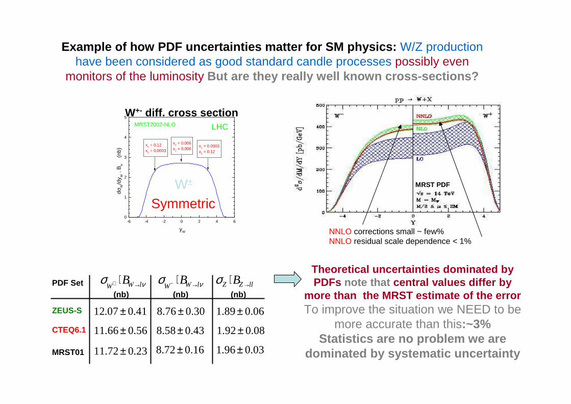
W±

Symmetric

W+- diff. cross section

Theoretical uncertainties dominated by PDFs note that central values differ by

more than the MRST estimate of the errorTo improve the situation we NEED to be

more accurate than this:~3%Statistics are no problem we are

dominated by systematic uncertainty

PDF Set

ZEUS-S

CTEQ6.1

MRST01

νσ lWWB →⋅+ νσ lWW

B →⋅− llZZ B →⋅σ

41.007.12 ±(nb) (nb) (nb)

30.076.8 ± 06.089.1 ±

56.066.11 ± 43.058.8 ± 08.092.1 ±

23.072.11 ± 16.072.8 ± 03.096.1 ±

Example of how PDF uncertainties matter for SM phys ics: W/Z production have been considered as good standard candle processes possibly even

monitors of the luminosity But are they really well known cross-sections?

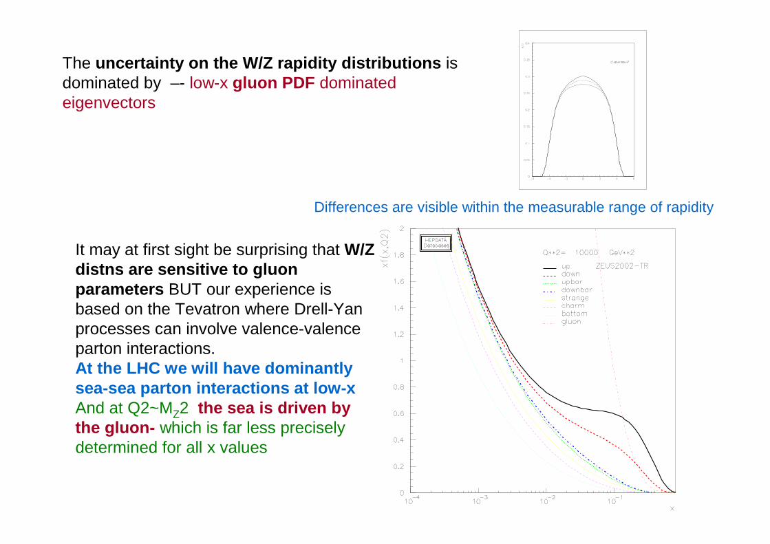
The uncertainty on the W/Z rapidity distributions is dominated by –- low-x gluon PDF dominated eigenvectors

It may at first sight be surprising that W/Z distns are sensitive to gluon parameters BUT our experience is based on the Tevatron where Drell-Yanprocesses can involve valence-valence parton interactions. At the LHC we will have dominantly sea-sea parton interactions at low-xAnd at Q2~MZ2 the sea is driven by the gluon- which is far less precisely determined for all x values

Differences are visible within the measurable range of rapidity

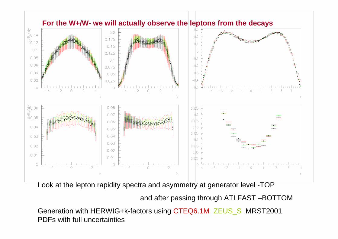
Look at the lepton rapidity spectra and asymmetry at generator level -TOP

and after passing through ATLFAST –BOTTOM

Generation with HERWIG+k-factors using CTEQ6.1M ZEUS_S MRST2001 PDFs with full uncertainties

For the W+/W- we will actually observe the leptons f rom the decays

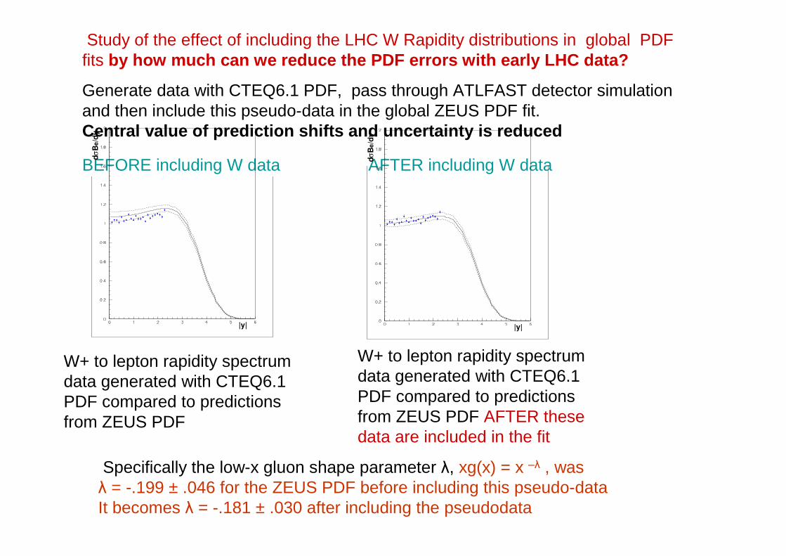
Study of the effect of including the LHC W Rapidity distributions in global PDF fits by how much can we reduce the PDF errors with early LHC data?

Generate data with CTEQ6.1 PDF, pass through ATLFAST detector simulation and then include this pseudo-data in the global ZEUS PDF fit.Central value of prediction shifts and uncertainty is reduced

W+ to lepton rapidity spectrum data generated with CTEQ6.1 PDF compared to predictions from ZEUS PDF

BEFORE including W data AFTER including W data

W+ to lepton rapidity spectrum data generated with CTEQ6.1 PDF compared to predictions from ZEUS PDF AFTER these data are included in the fit

Specifically the low-x gluon shape parameter λ, xg(x) = x –λ , wasλ = -.199 ± .046 for the ZEUS PDF before including this pseudo-dataIt becomes λ = -.181 ± .030 after including the pseudodata

|y|

dσ

Be/d

y

|y|

dσ

Be/d

y

LHC is a low-x machine (at least for the early years of running)

Low-x information comes from evolving the HERA data

Is NLO (or even NNLO) DGLAP good enough?

The QCD formalism may need extending at small-x

BFKL ln(1/x) resummation

High density non-linear effects etc.

(Devenish and Cooper-Sarkar, ‘Deep Inelastic Scattering’, OUP 2004, Section 6.6.6 and Chapter 9 for details!)

Thorne will talk about this

MRST have produced a set of PDFs derived from a fit without low-x data –ie do not use the DGLAP formalism at low-x- called MRST03 ‘conservative partons’. These give VERY different predictions for W/Z production to those of the ‘standard’ PDFs.

MRST02

MRST03

Z

Z

W+

W+

W-

W-

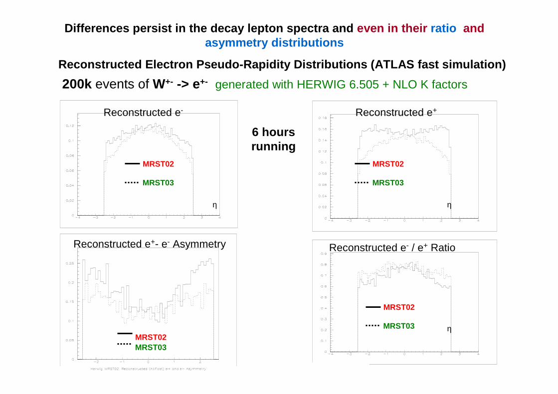
Reconstructed e- Reconstructed e+

Reconstructed e- / e+ Ratio

MRST02

MRST03

MRST02

MRST03

MRST02MRST03

η

η

η

Reconstructed e+- e- Asymmetry

MRST02

MRST03

Reconstructed Electron Pseudo-Rapidity Distribution s (ATLAS fast simulation)

200k events of W+- -> e+- generated with HERWIG 6.505 + NLO K factors

Differences persist in the decay lepton spectra and even in their ratio and asymmetry distributions

6 hours running

Note of caution. MRST03 conservative partons DO NOT describe the HERA data for x< 5 10-3 which is not included in the fit which produces them. So there is no reason why they should correctly predict LHC data at non-central y, which probe such low x regions.

What is really required is an alternative theoretical treatment of low-x evolution which would describe HERA data at low-x, and could then predict LHC W/Z rapidity distributions reliably – also has consequences for pt distributions.

The point of the MRST03 partons is to illustrate that this prediction COULD be very different from the current ‘standard’ PDF predictions. When older standard predictions for HERA data were made in the early 90’s they did not predict the striking rise of HERA data at low-x. This is a warning against believing that a current theoretical paradigm for the behaviour of QCD at low-x can be extrapolated across decades in Q2 with full confidence.

→ The LHC measurements may also tell us something new about QCD

Parton distributions are extracted from NLOQCD fits to DIS data- But they are needed for predictions of all cross-sections involving hadrons.

I have introduced you to the history of this in order to illustrate that it’s not all cut and dried- our knowledge evolves continually as new data come in to confirm or confound our input assumptions

You need to appreciate the sources of uncertainties on PDFs – experimental, model and theoretical- in order to appreciate how reliable predictions for interesting collider cross-sections are.

At the LHC high precision (SM and BSM) cross section predictions require precision Parton Distribution Functions

We will improve our current knowledge from the HERA data, and the Tevatrondata, before the LHC turns on

We can begin LHC physics by measuring ‘standard candle’ processes which are insensitive to PDF uncertainties

We can even use early LHC measurements, at low scales where BSM physics is not expected, to increase precision on PDFs and thus improve limits for discovery physics

But there is some possibility that the Standard Model is wrong not due to exciting exotic physics, but because the standard QCD framework is not fully developed at small-x, hence we may first learn more about QCD!

Summary