collection and interpretation of pavement structural ... · pavement structural parameters using...

Collection and Interpretation of

Pavement Structural Parameters using Deflection Testing

ParT II: ProjeCT level

March 2013

Tonkin and Taylor

Collection and Interpretation of

Pavement Structural Parameters using Deflection Testing

ParT II: ProjeCT level

March 2013

4 ColleCtion and interpretation of pavement StruCtural parameterS uSing defleCtion teSting part ii: projeCt level

abbreviaTions

ac Asphaltic Concrete

arrb Australian Road Research Board

cbr California Bearing Ratio

caPTiF Canterbury Accelerated Pavement Testing Indoor Facility

eLMoD Evaluation of Layer Moduli and Overlay Design

esa Equivalent Standard Axles

FLea Finite Layer Elastic Analysis

FWD Falling Weight Deflectometer

GMP General Mechanistic Procedure

hsD High Speed Data

hWD Heavy Weight Deflectometer

iri International Roughness Index

LWD Light Weight Deflectometer

LTPP Long Term Pavement Performance

Mesa Millions of Equivalent Standard Axles

naasra National Association of Australian State Road Authorities

nDM Nuclear Density Meter

nZTa NZ Transport Agency

Qa Quality Assurance

rLT Repeated Load Triaxial

rWD Rolling Wheel Deflectometer

shrP Strategic Highway Research Program

TsD Traffic Speed Deflectometer

WMaPT Weighted Mean Annual Pavement Temperature

5ColleCtion and interpretation of pavement StruCtural parameterS uSing defleCtion teSting part ii: projeCt level

conTenTsabbreviations 4

1. inTroDucTion 7

1.1 General 7

1.2 Network versus Project Level Evaluation 7

2. DeFLecTion TesTinG 9

2.1 General 9

2.2 Falling Weight Deflectometer 10

2.3 Heavy Weight Deflectometer 10

2.4 Light Weight Deflectometer 11

2.5 Deflection Testing Equipment Comparison 12

2.5.1 Austroads Correlations 12

2.5.2 Correlation between FWD and Instrumented Beam 13

2.5.3 Correlation between FWD and LWD 17

2.6 Accuracy 17

3. FWD TesT ProceDures 18

3.1 General 18

3.2 Loading 18

3.3 Selecting Offset Distances 18

3.4 Sampling Intervals 18

3.5 Field Recording 19

3.6 Unbound Basecourse with Chip Seal Surfacing 20

3.7 Asphaltic Concrete 20

3.8 Seal Extension 20

3.9 Widening, New Construction and Construction Monitoring 20

4. QuaLiTy assurance anD DeFLecTion boWL FieLD inTerPreTaTion 21

4.1 Repeatability 21

4.2 Rational Deflection Bowl Shapes 21

4.3 Surface Moduli Plot, Subgrade Modulus, CBR and Soil Type 21

5. PaveMenT DeFLecTion MechanisTic anaLysis 25

5.1 General 25

5.2 Data requirements 25


5.3 Pavement Analysis Methodology 26

5.3.1 Preliminary (Inferred Layer) Pavement Analysis 26

5.3.2 Finalised (Recorded Layer) Pavement Analysis 27

5.4 Software 27

5.4.1 General 27

5.4.2 EFROMD2 and CIRCLY 28

5.4.3 MODULUS 28

5.4.4 ELMOD 28

5.5.5 Limitations and Advantages of Software Features 29

5.5 Layer Moduli 32

5.5.1 Basic Calculations 32

5.5.2 Dependence of Moduli on Layer Thicknesses 33

5.5.3 Validity of Back-Calculated Elastic Pavement Material Properties 34

5.5.4 Unbound Granular Materials 34

5.5.5 Relating In situ FWD or Laboratory Moduli to CBR and DCP 37

5.5.6 Moduli of Stabilised Basecourses in New Zealand 41

5.5.7 Seasonal Effects 42

5.5.8 Layer Thickness Sensitivity 43

5.5.9 Rigid Base Condition 44

5.5.10 Anisotropy 44

6. rehabiLiTaTion TreaTMenT: MechanisTic DesiGn 47

6.1 General 47

6.2 Mechanistic Diagnosis of Pavement Distress 48

6.3 Unbound Granular Pavement Rehabilitation 49

6.4 Basecourse Stabilisation 50

6.5 Presentation 52

6.6 Design Review 55

7. MechanisTic DesiGn: neW PaveMenTs 56

7.1 Unbound Granular Pavements 56

7.2 Pavements with Multiple Bound Layers 58

8. consTrucTion QuaLiTy assurance anD DesiGn LiFe veriFicaTion 59

8.1 Predicting Design Life 59

8.2 Application 60

9. bibLioGraPhy 64


1. introduction1.1 GeneraLPavement deflection testing is undertaken as the primary means for establishing structural parameters. Part I of this set of two reports discusses “Network Level” deflection testing for asset management purposes. This report, Part II, addresses “Project Level” testing and interpretation for rehabilitation treatment of specific road lengths, or quality control during construction. Typical parameters established from deflection testing on New Zealand roads, including the NZ Transport Agency’s (NZTA) Long Term Pavement Performance (LTPP) benchmark sites, are presented.

The Falling Weight Deflectometer (FWD) allows rapid non-destructive structural evaluation of pavements. Where less accuracy and limited bowl profiles are required, the Benkelman Beam or Deflectograph may be utilised. Also in some countries (particularly the United Kingdom and Italy), national standards have been developed for the more portable Light Weight Deflectometer (LWD).

Obtaining deflection data at highway speed has been attempted seriously since about 2000; with the Rolling Wheel Deflectometer (RWD) in the United States, and more recently the Danish Traffic Speed Deflectometer (TSD). As the FWD is regarded as the benchmark for structural testing (in view of its inherently greater accuracy), it is the focus of this Guide.

Much of the material in this report was originally prepared for mechanistic design lectures for pavement rehabilitation given when deflection testing (measuring the full deflection bowl) was first introduced to New Zealand in the early 1990’s in conjunction with Transfund1 research. This update includes subsequent developments and findings from FWD deflection testing of New Zealand pavements over the last 20 years.

1.2 neTWork versus ProjecT LeveL evaLuaTionNetwork level management is concerned with the present and future condition of roading assets. The reason for determining the pavement structural condition throughout each network is to determine pavement life expectancy and maintenance requirements. This level of testing is discussed in detail within Part I of this series and is mainly concerned with more widely spaced tests throughout the full roading network with resulting lower level of scrutiny when compared to project level testing.

Part II of the series is focused on individual lengths of pavement that have reached a terminal condition and require rehabilitation, or have been recently treated and structural evaluation is required as a quality control tool for contractual reasons. New Zealand studies of case histories for new construction projects demonstrate the effectiveness of the FWD in this context (Section 7). The intensity of the analysis applied also sets project level analysis apart from network level analysis: project level analysis, for instance, also requires more detail regarding layer thicknesses, prior traffic volumes, as well as the intended design traffic.

The distinction between network and project level testing is discussed further by Austroads2 in Section 2, Part 5 of the Guide to Pavement Technology: Mechanistic Design.

1 Transfund was the precursor to the current New Zealand Transport Agency (NZTA). 2 Austroads is the association of Australian and New Zealand road transport and traffic authorities.


Austroads and the NZTA have adopted the mechanistic design procedure for pavement rehabilitation treatments.3

Mechanistic design typically involves using computer software (such as CIRCLY4) to analyse the reaction of various pavement layer configurations (modelled as multiple layers of linear elastic materials) under a standard wheel load. Some programs (such as ELMOD5) include allowance for non-linear elastic material or more generalised behaviour with finite element methods. The acceptable designs are those that meet or exceed specific performance criteria for asphalt, cemented or unbound granular layers and the subgrade.

Mechanistic design allows a range of rehabilitation treatments to be designed. These include strengthening the existing pavement layers (stabilisation), granular overlay, asphalt overlay, or any combination of these.

The requirement to determine each pavement layer’s elastic material properties for mechanistic design is now a principal issue for pavement designers. Measuring deflection bowls provides a simple and cost effective means of establishing the relevant properties.

Most overseas documentation on deflection testing relates to structural asphaltic pavements. This Guide draws on local experience with unbound granular pavements used in roads throughout New Zealand, as well as documentation from various local and international sources.

3 Austroads Guide to Pavement Technology (2011-2012) Pavement Part 2 – Section 8.4 CIRCLY (Mincad Systems 2004) -refer to section 6.3.2 of this report.5 ELMOD® (Evaluation of Layer Moduli and Overlay Design) – refer section 5.2.4 of this report.


2. Deflection Testing 2.1 GeneraLBack-analysis of a measured deflection bowl is a widely accepted method for estimating the existing pavement materials’ elastic properties - this is required for undertaking the rehabilitation treatments’ mechanistic design. Both the FWD and instrumented Benkelman Beam are used in New Zealand to measure the deflection bowl. The instrumented Beam, LWD, Deflectograph and TSD are briefly mentioned in this report for comparison with the FWD.

The FWD developed from the déflectométre à boulet originally devised by Bretonniere.6 A force pulse applied to the road surface by a specially designed loading system representing the dynamic short-term loading of a heavy wheel load. This produces an impact load of 25-30 ms duration, and a peak force of up to 120 kN (adjustable). The pavement’s deflection bowl response is measured with a set of nine precision geophones at a range of distances from the loading plate.

The Benkelman Beam, instrumented for automatic recording of the full bowl shape, measures responses under a slower and variable loading time. As the wheel load is positioned close to the point of maximum deflection during set up, the effective load duration is longer at close offsets than at the more distant points.

The Deflectograph is, in essence, a pair of automated Benkelman Beams mounted under a truck. This enables point testing at user-specified locations in the outer and/or inner wheel paths.

The LWD is a portable device that applies the same type of stress pulse acting on a 300 mm diameter plate (similar to the FWD), but the maximum stress is generally not greater than 200 kPa, and usually only the central deflection is measured - however, some devices now include additional offset geophones. There are two testing styles: the first measures the deflection of the plate under the impact of a known weight with known drop height, while the second has a small hole in its centre (as per the FWD) so that the central geophone is in direct contact with the soil, and a load cell records the stress pulse.

Austroads7 discusses in detail the relative attributes of the FWD, Benkelman Beam and Deflectograph.

The RWD and TSD have the advantage of speed and reading frequency, however initial models could not accurately define the full deflection bowl. Furthermore, they produced useable accuracy for peak deflection only by averaging a large number of readings along the wheeltrack. Results are obtainable only along straight sections of road, although improvements are steadily being made to remove this limitation. The RWD/TSD method is expected to become an effective network evaluation tool. It is discussed further in Part I of this Guide.

6 Bretonniere, S. (1963). Etude d’un deflectometre a boulet.7 Austroads Guide to Pavement Technology (2008-2009) Part 5, Section B.4.


2.2 FaLLinG WeiGhT DeFLecToMeTer The Falling Weight Deflectometer (FWD) is currently the most practical system for accurately measuring a pavement’s deflection response when it is subject to a dynamic load. It uses a set of weights, which may be dropped from various heights onto a load-cell-incorporated circular loading plate that has a number of geophones (deflection sensors) spaced in a line radiating out from the point of impact.

Figure 2.1 - The FWD trailer showing deflection bowl recorded at geophone offsets.

The geophones determine the deflection bowl produced by the falling weight’s impulse. These data, combined with the measured impact load, may be back-analysed (using layered elastic theory) to determine the stiffnesses (e.g. dynamic moduli – E1, E2) of the various layers, and the subgrade (ESG).

2.3 heavy WeiGhT DeFLecToMeTerThe Heavy Weight Deflectometer (HWD) operates on an identical principle to the FWD, but with additional weights for simulating higher loads typically required of heavy duty pavements. It is capable of applying a dynamic force, depending on the stiffness of the pavement structure, of up to approximately 240 kN. The HWD can be configured to produce similar impulse loading as the FWD, but it is important to apply appropriate filtering and calibration to FWD.


2.4 LiGhT WeiGhT DeFLecToMeTerThe Light Weight Deflectometer (LWD) is becoming used increasingly in the United Kingdom and Italy, particularly for new pavement construction. When testing on a stripped subgrade or lower subbase, the stress level applied by the LWD should generally be comparable with the eventual in-service vertical stress expected from a 1 Equivalent Standard Axle (ESA) loading after load spread through the upper layers, although the confining stresses will be less for the LWD. The United Kingdom standard IAN73, indicates that the modulus for LWD tests will be a partially confined value. For unbound materials, this can be approximately 60% of that expected when confined beneath a finished pavement. For this reason, the LWD may then have a relevant role in new pavement construction when checking design moduli assumptions. The LWD was found to be of use as a QA tool, but inherent sources of difference needed to be kept in mind by operators and analysts when validating and applying the test results. These included the variable number of seating blows, variable plate-ground contact, and lower test impulses.

Early LWD testing (e.g. once stripping to subgrade level has been done) can quickly identify (in relative terms at least) where any local soft spots are and can help quantify any necessary depth of undercut; thus it provides an additional QA tool for stiffness measurement, particularly when testing during construction, directly on the subgrade or subbase. It should not be regarded as a substitute for compaction testing, but rather as an additional tool because it will quickly indicate the areas of any layer that should be included for focussed nuclear density testing (NDM).

If possible, expected target values for layer moduli and deflection values should be recommended in advance of testing. This enables the LWD operator to appropriately set up the test impulse by altering the drop height or plate size. Full time histories of the peak deflection and response should ideally be electronically recorded and immediately reviewed after the test to ensure an adequate impulse has been produced and a meaningful result has been obtained.

To overcome limitations of the LWD regarding plate-ground contact, current practice in the United Kingdom includes measures such as removing the top 100 mm of material prior to testing, using the LWD on a maximum gradient of 5%, and spreading a thin bedding layer of moist sand between the LWD and testing surface.


Figure 2.2 - The LWD device configuration.

2.5 DeFLecTion TesTinG eQuiPMenT coMParison2.5.1 austroads Correlations

Table 2.1 describes the comparative means of finding:

§ Standardised central deflection (D0),

§ Standardised deflection at 200 mm offset (D200)

§ Curvature function (D0 – D200).

ParaMeTer FWD DeFLecToGraPh benkeLMan beaM

Central Deflection (D0) Maximum recording taken at each test site.

Total deflection minus residual deflection (which is the rebound deflection, see Figure 2.3).

Deflection Bowl & Curvature Function (CF)

The deflection bowl is measured directly.

Estimated using the principle of superposition from a series of deflection readings taken at a specific point on the pavement as the load approaches or recedes from that point.*

* For example, the deflection at a point 200 mm from the point of maximum deflection is assumed equal to the deflection at a specific test point when the moving test load is 200 mm away. The shape of the deflection bowl is obtained by plotting recorded deflection against the distance between the test point and the load for a series of positions of the load.

Table 2.1 - Comparison between FWD, Deflectograph and Benkelman Beam.


Figure 2.3 - Maximum, standard and residual (Benkelman Beam) deflection.8

2.5.2 Correlation between FWD and Instrumented Beam

The ideal duration of a pavement test load should correspond to that of a moving wheel at a velocity of 60 to 80 km/hr. The velocity is important because it affects the load duration (and therefore the measured deflections) which relates to the visco-elastic characteristics of any asphalt layers and the elasto-plastic response of the subgrade.

The response of the pavement structure to the FWD, Beam and to loading by a moving wheel load has been compared on several instrumented test roads.9 In that research, stresses, strains and deflections were measured under comparative conditions. Because of the FWD loading system’s design, the responses under the FWD and moving wheel load are practically identical. On the other hand, Ullidtz’s study has shown that no simple correlation exists between the Benkelman Beam and the moving wheel load. The relation is very dependent upon the specific visco-elastic responses governed by the asphalt layers’ and subgrade’s dynamic characteristics.

Therefore, if the deflection bowl is measured under an FWD test, with the theory of elasticity then being used to determine the moduli of the individual layers, a useable model can be developed. The resulting layer moduli will then be representative of the pavement materials under moving traffic loads. Because of its longer loading period, the instrumented Benkelman Beam cannot be used as directly as this.

Using a dynamic loading device is clearly preferable. Ideally, the analysis should also be dynamic and research has been continuing into this aspect. As yet, however, there is no widely used dynamic analysis procedure – partly because of the computational time required10. As long as the current form of pseudo-static analysis is used for establishing stresses and strains, there is little practical benefit in using more rigorous static analysis methods. However, when dynamic analysis methods come into common use, it will then be necessary to abandon the traditional static analysis strain criteria and develop a new set calibrated to the dynamic analyses.

There is no universal comparison. This is because the ratio of Benkelman Beam to FWD central deflection is a function of the pavement composition (elastic properties of the pavement materials and the subgrade). It is however possible to obtain consistent ratios on any one pavement type.

8 Austroads Guide to Pavement Technology (2008-2009). Pavement Part 5 figure B.4.9 Ullidtz, Per (1973). En studie af to dybdeasfaltbefaesterlser.10 Ullidtz, P. & Coetzee, N.F. (1995). Analytical Procedures in Non-destructive Testing Pavement Evaluation.


Paterson11 reports:

» The loading applied by FWD is currently considered to be more similar to traffic loading in both the load and the time domains than either the Benkelman Beam test (which applies similar loads at creep speed) or the light-loading, high frequency devices. Under similar applied loads, the ratio of FWD to Benkelman Beam deflections ranges from 0.8 to 1.35 for asphalt-surfaced pavements. Thus a reasonable first approximation, in the absence of specific local correlations, is to equate FWD deflection (after correction for the applied load) to the Benkelman Beam deflection.

Paterson apparently drew his conclusions from the work of Tholen et al.12 who collated data from a number of projects using different pavement types, but found no systematic correlation.

A comparison between the central deflections measured by the Benkelman Beam and FWD is important in order that the substantial body of experience and empirical relationships obtained with the Benkelman Beam can be carried forward. The simplified methods can still be used as a broad check on interpretations made using the full deflection bowls measured by either the FWD or Instrumented Beam.

To examine the theoretical relationship between the two loading devices, calculation checks were undertaken using CIRCLY and the finite element program FLEA13 .

A 40 kN load was initially applied to two discrete circles spaced 330 mm between centres, and the deflection was calculated midway between the loads to simulate the dual wheels of a Benkelman Beam truck. The same 40 kN load was then applied over a 300 mm circular area with a central hole to simulate the FWD loading plate. The deflections between the dual wheels and directly under the FWD loading plate were computed for comparison.

Both methods of analysis produced a theoretical Beam: FWD ratio of much less than 1 (slightly dependent on layer moduli). This was a surprising result in view of the generally accepted higher correlations. It is important to appreciate that these analyses relate to a continuum (i.e. a material that is continuous rather than the assemblage of discrete particles as found in a granular layer). Therefore, the theoretical results may be expected to be more appropriate to very dense pavements (with low deflections) than unbound granular layers.

As part of ongoing research in New Zealand, Beam:FWD ratios were also determined for one unbound granular pavement with thin friction course surfacing, and one structural asphaltic pavement at the Canterbury Accelerated Pavement Testing Indoor Facility (CAPTIF) test track. The results gave Beam:FWD ratios of 1.05 and 1.22 respectively. The CAPTIF data, obtained from research at the University of Canterbury, allowed precise positioning of both Beam and FWD, and produced a high correlation.

Using data from Tholen et al.12, together with local information, there appears to be a slight trend for greater Beam:FWD ratios with greater overall deflection (Figure 2.4 - Comparison of Benkelman Beam and FWD central deflections (using a 40 kN load).). This result is not expected when the difference between the loading times and mass-inertia effects are considered. This result is discussed in Section 3.4.

11 Paterson, W.D.O (1987). Road Deterioration and Maintenance Effects.12 Tholen, O., Sharma, J. & Terrel, R.L (1985). Comparison of Falling Weight Deflectometer with other

Deflection Testing Devices.13 FLEA (Finite Element Programme,University of Sydney 1994).


Figure 2.4 - Comparison of Benkelman Beam and FWD central deflections (using a 40 kN load).

The data support others’ conclusions that there is no real correlation (even when plotted logarithmically), and site-specific correlations should be undertaken. Ideally, this correlation should be made by direct reading. Indirect correlations could be carried out using a program such as CIRCLY, FLEA or ELMOD, but limited experience suggests that such theoretical approaches can yield Beam:FWD ratios that are lower than achieved in practice. As an interim guide, the following approximations taken from Figure 2.4 - Comparison of Benkelman Beam and FWD central deflections (using a 40 kN load). are suggested from New Zealand experience for unbound granular pavements with no thick structural AC.

Where deflections are less than 1 mm under a 40 kN FWD impact load, use:

Beam:FWD ratio = 1.1

Where deflections exceed 1 mm, the ratio is likely to be in excess of 1.1, and related to deflection as defined by:

Beam:FWD ratio = 1.1 x (FWD deflection in mm) 0.4 ( 1 )

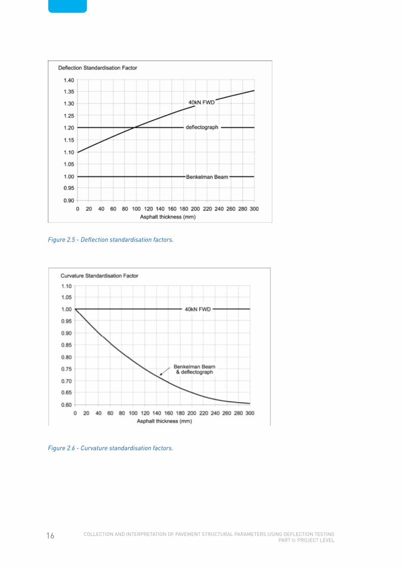
Austroads14 discusses the correlation between FWD, Deflectograph and Benkelman Beam and gives curves based on Australian experience (Figure 2.5 - Deflection standardisation factors. and Figure 2.6 - Curvature standardisation factors.) for AC pavements.

14 Austroads – Guide to Pavement Technology (2008-2009). Part 5 Section E.2, figures E.3 and E.4.


Figure 2.5 - Deflection standardisation factors.

Figure 2.6 - Curvature standardisation factors.


2.5.3 Correlation between FWD and lWD

The LWD loading system is conceptually the same as the FWD. In theory, the same stress and central deflection should be obtainable if the same drop weights, buffers, and plate size are used (see Figure 2.2 - The LWD device configuration.).

Intuitively, changing one or more of the weight, buffer resilience or plate size characteristics will affect the test impulse load; therefore particular attention when comparing results should be paid to ensuring the LWD setup is identical to the FWD setup. If there are even slight differences in the resulting stress pulses, then calibration will be needed. Differences in material composition, compaction state, layer thickness and so on should also be accounted for when correlating test results of different sites or test methods.

The Dynatest LWD routinely uses the same plate size (300 mm) as the FWD, but the plate stress is generally of a lesser magnitude making it less suitable for effective testing of completed (full depth) pavements. Where the layer moduli are stress dependent (explained in further detail in section 4.3), the LWD is likely to over-predict moduli for cohesive soils and under-predict the moduli for thick granular layers (assuming the FWD test stress is representative of the in-situ stress under in-service traffic). Unless the LWD can impose realistic stresses and strains at depth (comparable to maximum traffic loadings), the accuracy of the device will be debatable.

2.6 accuracyBecause no reference point or support is needed for FWD deflection bowl measurement, the deflections can be measured with high accuracy. Ullidtz15 indicates a typical accuracy of 0.5% ± 1 µm. This accuracy is necessary because the subgrade modulus must often be determined from deflections of only 20-30 µm. The accuracy of the geophones can be readily checked at any time in the field by setting all sensors vertically above one another in a special test frame (tower) to confirm identical amplitudes and responses.

The accuracy of deflections is further ensured by carrying out measurements at least two or three times at each point to assess repeatability. This will allow the effects of different loadings to be evaluated and identify any external factors that may have affected results, such as passing vehicles, or the effects of loose surfacing. Thick structural AC pavements are usually tested three times at each point. Aged unbound granular pavements with thin seal surfacings tend to compact progressively with each blow, so results appear considerably more favourable after multiple blows. To assess the actual condition more realistically, a limit of two tests at any one location is preferable with these pavements.

Calibration is carried out on a monthly basis (relative calibration of all deflection sensors) and annually for reference calibration. Both European and United States protocols for calibration have been carried out in New Zealand. Further information is available on the US Department of Transportation website.16

The Benkelman Beam test has somewhat lesser accuracy and repeatability in practice, owing to the effects of proximity of its supporting legs, load reversal and accuracy in repositioning. Because usually only one beam test is done at each test point, there is no verification or easy means of checking for faulty tests (such as when the probe tip has been dislodged during the test without the tester being aware of the fact).

15 Ullidtz, Per (1987). Pavement Analysis.16 http://www.fhwa.dot.gov/publications/research/infrastructure/pavements/ltpp/07040/index.cfm

http://www.fhwa.dot.gov/publications/research/infrastructure/pavements/ltpp/07040/index.cfm


3. FWD Test Procedures

3.1 GeneraLDuring a normal FWD operation, the total test sequence is controlled from the front seat of the towing vehicle. Results are automatically stored electronically for subsequent uploading and processing. Typically 200 to 300 points may be tested during one day, i.e. up to 15 lane kilometres of testing at project level (50 m centres), or more for network level appraisals.

3.2 LoaDinGThe FWD load is normally adjusted in the field to between 35 and 50 kN, to produce maximum deflections towards the upper limit of the geophone capacity (i.e. about 2 mm). Results are then standardised to a 40 kN load (or adjusted to Benkelman Beam values as discussed above). Alternatively, as at least one seating load pulse and two or three recordings are made at each site, a sequence of 35, 40 and 50 kN impacts may be automatically applied to examine stress dependence more closely. The effective impact can be altered by varying the drop height (determined by a set of proximity sensors manually placed next to the falling weight guide mechanism), or by specifically defining target loads in the field program.

For heavy-duty pavements, higher loads may be specified (up to about 240 kN).

3.3 seLecTinG oFFseT DisTances On the FWD, geophones are clamped in the required positions at the desired offset from the centre of the loading plate. For the instrumented Benkelman Beam, progressive recording of offsets is required.

Recommended offset distances for determining a pavement’s elastic properties depend on the pavement layers’ overall stiffness. For a typical New Zealand unbound granular pavement, deflections should be recorded at: 0, 200, 300, 450, 600, 750, 900, 1200 and 1500 mm distances from the centre of the load.

For very thick granular pavements, cement-stabilised basecourses, or thick asphaltic concrete pavements, greater spacings may be required. This will ensure the three outermost measurement points are positioned to obtain a subgrade response (as explained in Section of this report).

If bowl shapes are required at different offsets, specific values may be determined using curvilinear interpolation (e.g. the Lagrange method), provided the full bowl shape is reflected about the y axis, and with the assumption that the central deflection occurs continuously over a 60 mm radius circle.

3.4 saMPLinG inTervaLsProject level testing is carried out for either pavement structural rehabilitation, or for undertaking quality assurance on a new construction. The standard spacing of FWD tests is 50 m centres in the left wheeltrack of each lane (staggered across lanes), with additional tests on any highly distressed locations at the discretion of the operator. A minimum of 30 tests in any one section is recommended to reliably assess the 5th or 10th percentile parameters usually adopted for design or acceptance testing.


3.5 FieLD recorDinGBy default, the FWD records the maximum impact load from a stress sensor above the loading plate and the peak deflection bowl from the geophone sensors.

The FWD may also be configured to record the full time history of stress and deflection by sampling each of the sensors at 0.1 millisecond intervals (an example is shown below in Figure 3.1 - Typical FWD record of geophone displacement (microns) v. time (milliseconds).).

2000

1500

1000

500

0

-500

Plate Stress

Deflection d600

Deflection d0

Deflection d750

Deflection d200

Deflection d900

Deflection d300

Deflection d1200

Deflection d450

Deflection d1500

Time (milliseconds)

Full Time History

Pla

te S

tres

s (k

Pa)

and

Def

lect

ion

(mic

rons

)

10 20 30 40 50

Figure 3.1 - Typical FWD record of geophone displacement (microns) v. time (milliseconds).

This test on a thin unbound granular pavement shows the outer geophones hardly begin to respond before the stress pulse reduces to almost zero. It is clear that the mass inertia of the pavement layers above the subgrade makes a significant contribution to the deflection bowl response to impact loading.

Considerable theoretical investigation of this effect, comparing the frequency response functions obtained from FWD load-time histories with those calculated using sophisticated elasto-dynamic models of layered systems, has been undertaken, but implementing these models for pavement design has proven too demanding for routine evaluation.10,17

Recent developments in processing FWD deflection data including the full time histories have provided simple methods for substantially increasing pavement performance prediction reliability.18 These methods are based on sampling the full FWD recording at 0.1 millisecond intervals, using one seating drop then two drops at 40 kN for chipseal or thin AC pavements, or one seating drop then three drops at 40 kN on thick structural AC. This should be standard practice where the principles of NZTA RR 401 are adopted. NZTA specify a target load of 650 kPa for some contracts (section 8).

17 Stolle D & Peiravian, F. (1996). Falling Weight Deflectometer Data Interpretation using Dynamic Impedance.18 Salt, G & Stevens D. (2010). Rationalisation of the Structural Capacity Definition and Quantification of

Roads based on Falling Weight Deflectometer Tests (NZTA Research Report 401) http://www.nzta.govt.nz/resources/research/reports/401/docs/401.pdf

http://www.nzta.govt.nz/resources/research/reports/401/docs/401.pdf

http://www.nzta.govt.nz/resources/research/reports/401/docs/401.pdf


3.6 unbounD basecourse WiTh chiP seaL surFacinGProject level testing of unbound basecourse is normally undertaken in the left wheelpath at 50 m intervals, or at shorter intervals where anomalies are detected. Closer spacing is also used on short sections in an attempt to obtain a minimum of 30 tests for analysis. When testing in the opposite lane, test locations are staggered evenly between those in the initial lane to allow pavement-wide coverage at 25 m centres.

With the FWD, at least two drops are undertaken at each site with checks made for repeatability, consistency of bowl shapes and surface moduli (discussed in Section 4).

Beam readings are not normally repeated, but test spacing may be closer (at 20 m in each lane) to compensate for this lack of repeatability.

3.7 asPhaLTic concreTeTesting AC or other bound asphaltic surfacing is similar to procedures for unbound basecourse. However, the temperature of the asphalt is measured regularly with results recorded in the FWD data file. Three drops per test site are recommended.

3.8 seaL exTensionTesting unsurfaced (loose gravel) roads or subgrades is quite practical with the FWD or LWD, because repeated tests are undertaken in quick succession until consistent results are obtained. Testing is the same as for unbound basecourses.

The Beam is limited to very firm surfaces, as local heave between the loaded dual wheels can readily invalidate results and repeat testing each site is not normally undertaken.

3.9 WiDeninG, neW consTrucTion anD consTrucTion MoniTorinG

Testing for widening is undertaken in the same way as for seal extensions, although testing is carried out in the area to be widened rather than in the existing wheelpath. Tests in the left wheelpath may also be useful for determining the effectiveness of the existing design in estimating likely equilibrium values for subgrade moduli beneath the new widening.

Similarly, for new construction or construction monitoring, testing is undertaken in the same way as for seal extensions. However, judgement regarding likely seasonal changes in subgrade stiffness is required during analysis.

New pavements also show relatively low moduli for the basecourse (and subbase) even though they may be thoroughly compacted. Further densification with substantial improvement in basecourse moduli will occur in an unbound granular pavement during the first 10,000 to 20,000 Equivalent Standard Axles (ESA) of trafficking. Somewhat longer trafficking may be required to achieve full densification beneath a structural asphaltic surfacing or in subbase materials.


4. Quality assurance and Deflection bowl Field interpretation

4.1 rePeaTabiLiTyRepeating tests in the same position is routinely undertaken for FWD surveys. Usually, results will be within a few per cent, i.e. inconsequential in relation to differences caused by a shift in test location of less than a metre (substantial variability over small distances is inherent in pavement materials). The FWD field program automatically displays the successive deflection bowls so anomalies can be identified on site. This also enables the test to be rejected and repeated until successive consistent readings are obtained prior to moving on to the next test location.

4.2 raTionaL DeFLecTion boWL shaPesA normal deflection bowl will have decreasing deflections with increasing distance from the load. The FWD field program alerts the operator at the time of the test if this criterion is not met, and the test may be rejected and repeated. Readings are also rejected if any of the geophone readings are affected by vibrations; these are occasionally significant when a heavy vehicle passes while the test is in progress.

4.3 surFace MoDuLi PLoT, subGraDe MoDuLus, cbr anD soiL TyPe

The most effective means for undertaking the field data’s quality assurance is to inspect the composite moduli plot corresponding to each test drop (these are displayed graphically by the FWD field program). The composite modulus is the “weighted mean modulus” of an equivalent half space of a material with uniform modulus. The concept of “overall apparent stiffness” at any point is important for the analyst’s understanding of the pavement, and for the designer.

The composite modulus (or “surface modulus” in European terms – which must not be confused with the modulus of a surface layer) is calculated from the surface deflections at each geophone using Boussinesq’s equations:

Eo(0) = 2 (1 - µ2) σo a / D(0) ( 2 )

Eo(r) = (1 - µ2) σo a2 / (r D(r)) ( 3 )

where:

Eo(r) = Surface modulus at a distance r from the centre of the loading plate, µ = Poisson’s ratio (usually set equal to 0.35) σo = Contact stress (assumed uniform) under the loading plate a = Radius of the loading plate, and D(r) = Deflection at the distance, r.

The central composite modulus Eo(0) (equation 2) is also used in the LWD test.


The subgrade modulus plot (Eo versus r) provides at the time of test:

§ An estimate for subgrade modulus (usually regarded as approximately equal to 10 x CBR)

§ Immediate determination of whether the subgrade modulus is linear elastic or non-linear, giving an indication of likely soil type

§ Confirmation of the geophone settings’ adequacy (as shown in the following three figures).

Figure 4.1 - Composite modulus plot with linear elastic subgrade modulus. shows an example of a composite modulus plot from a pavement with linear elastic subgrade, as evidenced by the outer three geophones showing essentially the same composite modulus (approximately 300 MPa). At relatively large distances (generally more than 600 mm) from the loading plate, all compressive strain will occur in the subgrade (rather than in the pavement layers, which lie outside the stress bulb). For this reason, the outer deflections will be uninfluenced by the pavement structure; the composite modulus will tend to the modulus of the subgrade alone. Linear elastic materials tend to be sands and gravels; the subgrade at this location is likely to be a compacted sand or gravel.

Figure 4.1 - Composite modulus plot with linear elastic subgrade modulus.

Figure 4.2 - Composite modulus plot with non-linear subgrade modulus. shows an example of a composite modulus plot from a pavement with moderately non-linear elastic subgrade. The three outer geophones show an apparently increasing modulus with increasing distance (i.e. decreasing stress). The subgrade modulus is approximately 80 MPa which, with the non-linear response, suggests a firm silt or clay.

Results showing moderate or high subgrade moduli, together with a highly non-linear response, may represent poor drainage at the top of the subgrade. Very low subgrade moduli, together with strongly non-linear responses, are indicative of soft clays or peat. The stress dependence of subgrade soils has been quantified by Ullidtz15, ELMOD19 in terms of a subgrade non-linearity exponent (n) which ranges from a value of 0 (for linear elastic soils) to -0.6 or less (for subgrades with highly non-linear moduli). Further details are given in Section 5.3.5.

19 Dynatest Engineering A/S (1989). ELMOD (Evaluation of Layer Moduli and Overlay Design) Users Manual.


Figure 4.2 - Composite modulus plot with non-linear subgrade modulus.

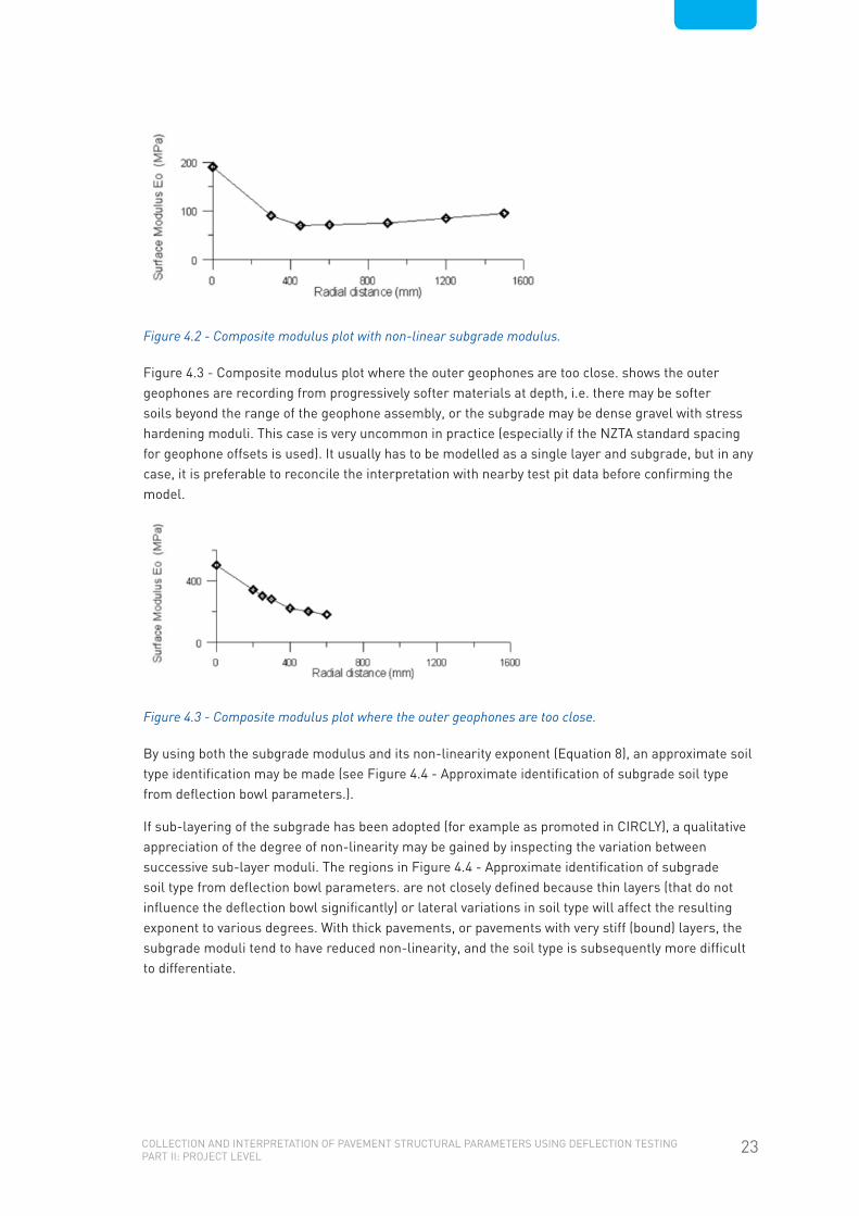
Figure 4.3 - Composite modulus plot where the outer geophones are too close. shows the outer geophones are recording from progressively softer materials at depth, i.e. there may be softer soils beyond the range of the geophone assembly, or the subgrade may be dense gravel with stress hardening moduli. This case is very uncommon in practice (especially if the NZTA standard spacing for geophone offsets is used). It usually has to be modelled as a single layer and subgrade, but in any case, it is preferable to reconcile the interpretation with nearby test pit data before confirming the model.

Figure 4.3 - Composite modulus plot where the outer geophones are too close.

By using both the subgrade modulus and its non-linearity exponent (Equation 8), an approximate soil type identification may be made (see Figure 4.4 - Approximate identification of subgrade soil type from deflection bowl parameters.).

If sub-layering of the subgrade has been adopted (for example as promoted in CIRCLY), a qualitative appreciation of the degree of non-linearity may be gained by inspecting the variation between successive sub-layer moduli. The regions in Figure 4.4 - Approximate identification of subgrade soil type from deflection bowl parameters. are not closely defined because thin layers (that do not influence the deflection bowl significantly) or lateral variations in soil type will affect the resulting exponent to various degrees. With thick pavements, or pavements with very stiff (bound) layers, the subgrade moduli tend to have reduced non-linearity, and the soil type is subsequently more difficult to differentiate.


Figure 4.4 - Approximate identification of subgrade soil type from deflection bowl parameters.

Further explanation on calculating non-linear stress dependence is given in section 5.4.1.

Because the composite modulus is computed directly (no layer information or back-calculation routines are required), this parameter can be readily inspected in the field as testing progresses.

Besides identifying soil type and possible subsurface drainage problems, an additional subgrade modulus plot function provides designers with quality control during processing. The composite modulus plot is normally inspected so irregular deflection bowl shapes can be rationally assessed and discounted if they are appropriate. It is usually straightforward to identify bowls that, for instance, have been located over a culvert or approach slab, or have one geophone suspended over a pothole.


5. Pavement Deflection Mechanistic analysis

5.1 GeneraLA large standardised central deflection usually indicates a thin pavement on a soft subgrade with associated rutting potential. The shape of the deflection bowl allows a detailed structural analysis of the pavement to be undertaken: the outer deflections define the subgrade stiffness, while the bowl shape close to the loading plate represents the stiffness of the near surface layers. A broad bowl with little curvature indicates the pavement’s upper layers are stiff in relation to the subgrade. Conversely, a bowl with the same central deflection but high curvature around the loading plate indicates that the moduli of the upper layers are relatively low. With the critical layer identified in this manner, existing or potential distress mechanisms can be identified, and therefore the most appropriate treatment may be determined and designed for.

5.2 DaTa reQuireMenTs The various categories of data for evaluating structural performance at project level, and their relative importance, are given in the following table. Ideally, all the items in italics should be provided to the pavement structural analyst, although as indicated below, the analyst can also deduce some of these.

1. Essential § FWD peak deflection data, peak plate stress

§ Pavement temperature at time of test (only used for asphaltic layers)

§ Nature and thickness of any bound layers (for new pavement QA and life prediction)

§ Traffic (ESA/lane/year) growth, lane distribution

§ Intended design life

2. Essential (but can be inferred by the FWD structural analyst)

§ Top structural layer type

§ Subgrade type (volcanic ash or otherwise)

3. Important (but can be identified or recorded by the FWD operator)

§ Surfacing type

§ Percentage of road in a terminal condition

§ Distress (approximate visual severity)

§ Full time history (dynamic record of all sensors while the FWD load is applied)

4. Preferable (but can be inferred by the FWD structural analyst)

§ Pavement profile (test pit logs, subgrade DCP)

§ Nature and thickness of any bound layers (for rehabilitation), or depth to subgrade (if only unbound granular layers)

§ Weighted mean annual pavement temperature (WMAPT °C)

5. Preferable (should be readily available in RAMM)

§ Dates of last construction and surfacing

§ Past traffic (ESA), or Future/Past traffic ratio

6. Desirable to verify model § HSD rut depths

§ HSD roughness (IRI or NAASRA counts)

Table 5.1 Information categories for pavement structural analysis.


For sites due for rehabilitation, precise pavement profiles are not always essential, however where there are bound layers, and QA of new construction is required, it is imperative that reliable as-built profiles are provided.

5.3 PaveMenT anaLysis MeThoDoLoGy5.3.1 Preliminary (Inferred layer) Pavement analysis

FWD data (pressures/deflections) are gathered in the field and processed by a pavement structural analyst. The data are corrected when there are obvious anomalies (usually due to non-uniformity of the pavement layering or unstable (cracked) surfacing) and then are back-analysed through appropriate software (such as Dynatest’s ELMOD20) to return a set of layer moduli. The resulting data are processed using a number of different routines to determine parameters (such as remaining life, structural number/indices, overlay and rehabilitation options) from which the analyst may make recommendations regarding the pavement’s current and future serviceability.

During the analysis phase, some understanding of the existing pavement structure is required. An iterative procedure adjusts the moduli of the layers to best match the input deflections for a nominated set of layer thicknesses; therefore, it is preferable that the model is derived from as-builts, and/or test pit observations stored within RAMM.

However, if neither exist, then a systematic preliminary analysis is adopted, trialling various layer thicknesses (this may be termed the “rational modular ratio” procedure for logically inferring probable layer thicknesses). Normally, the operator will record the pavement surface type in the field, but little else below the surface can be identified at the time of testing. In many highway situations where there clearly is a chip seal surfacing, an unbound granular pavement can be assumed initially. In that situation, the modulus of each unbound layer is dependent on the modulus of the underlying layer (as described in the Austroads Pavement Design Guide); the pavement layer thicknesses are adjusted and the back analysis of the multi-layer model is carried out iteratively until the Austroads modular ratios are satisfied. (These are the established values relating the modulus of each layer to the modulus of the underlying layer coupled with the specific layer thicknesses.) In this manner, the probable layering of unbound pavements can be inferred with reasonably good reliability.

From studies of the New Zealand national Long Term Pavement Performance (LTPP) sites, it has been established that the Austroads modular ratios are directly applicable to New Zealand conditions. The quantification has been found to be remarkably reliable, demonstrating the well-recognised practical viewpoint that the stiffness of any granular layer (how well it can be compacted) relates directly to how good an “anvil” is present beneath it.

If there is a bound layer forming the uppermost layer of the pavement, then the magnitude of the moduli of the top layer are governed by whether the layer is heavily bound (cemented or concrete), asphaltic concrete, lightly bound, or still in an effectively unbound state (lime/cement modified). In the latter case, the range of moduli may overlap those of untreated granular aggregates.

If any top layer moduli are unusually high, the analyst will need to revise any initial assumption that the top layer is unbound, and should make enquiries to determine if there is any knowledge of the layer type. If there are stiff intermediate layers (e.g. cement bound subbase), analyses can have low reliability. Such “upside down” pavements are relatively rare in New Zealand, and where they are present, there is usually good as-built information.

20 ELMOD® (Evaluation of Layer Moduli and Overlay Design) is a Dynatest licensed product.


5.3.2 Finalised (recorded layer) Pavement analysis

When as-built data or information from test pits is available (usually from RAMM), the model can readily be established at individual chainages that coincide with test pit locations. However, judgment is still required to establish where changes in layer thicknesses should be applied between the specific chainages where the profile is known. The modular ratios are used (using the principles described above) to find the transition points to use for the model layering (i.e. structural sectioning).

Typically, the relevant data stored in RAMM are simply Layer Type (surfacing, pavement layer or subgrade), Layer Thickness, and Depth to Subgrade. The data for each section may be developed into either a one, two or three layer model (depending on the total depth to subgrade), and the layer thicknesses adjusted after each iteration whilst maintaining the total pavement depth.

However, the inclusion of recorded pavement layer information may not necessarily produce a more realistic model. Further explanation is given in section 5.4.2.

5.4 soFTWare5.4.1 General

A large selection of software is now available for determining the stresses, strains and deflections within a layered elastic system. A back-analysis procedure is generally adopted to determine moduli from an observed deflection bowl. The iterative procedure adjusts the trial layer moduli until the computed deflection bowl approximates the measured deflection bowl. When the multi-layered elastic model is established, forward-analysis is undertaken to determine strains for use in rehabilitation treatment designs. Some packages (e.g. EFROMD221, EVERCALC, PADAL, and CIRCLY) are supplied as separate programs, while others (eg. ELMOD) combine both back- and forward-analyses into a single program.

Ullidtz & Coetzee10 summarise the properties of several back-calculation programs. Most of the forward analysis programs (including CIRCLY, BISAR22 and MODULUS23) are based on multi-layer elastic theory with numerical integration or finite element analysis (e.g. FLEA), while a few (eg. ELMOD) include options for the very rapidly executing Odemark-Boussinesq transformed section approach, which are popular due to their reduced processing time.

Comparisons of the results obtained for the same deflection data analysed with different programs are given by Lytton24 and Ullitdz.15 The adopted seed moduli can affect outcomes but most differences will arise from the operator’s choice of consistent layer thicknesses. Any misjudgement in the adopted layer thicknesses during back-analysis will tend to cancel out when determining overlay thickness during forward-analysis, however appropriate model layering is important when evaluating likely distress mechanisms. Features and advantages of some software packages are discussed in Section 5.3.5.

21 EFROMD2 - Pavement Analysis programme developed by the Australian Road Research Board (ARRB) – refer to section 6.3.2. of this report.

22 BISAR –Pavement Analysis programme as discussed within the Shell Pavement Design Manual.23 MODULUS - (Texas Transportation Institute) refer section 6.3.3 of this report.24 Lytton, R L, (1988). Backcalculation of Pavement Layer Properties, Nondestructive Testing of Pavements and

Backcalculation of Moduli.


5.4.2 eFroMD2 and CIrClY

The Australian Road Research Board (ARRB) developed EFROMD2. It uses CIRCLY iteratively to provide elastic layer moduli corresponding to a given deflection bowl.

Field data from either the FWD or Instrumented Benkelman Beam may be used, and the program will apply one or two loading circles accordingly. The program also corrects for secondary effects if the beam support points are affected by the deflection bowl.

When an appropriate model of the existing pavement is established, CIRCLY is used again in the forward analysis to evaluate rehabilitation options. For materials where the modulus is strongly dependent on stress levels, sublayering is recommended to improve modelling accuracy.

Seed moduli are required for EFROMD2, and maximum/minimum credible moduli can be specified. CIRCLY uses numerical integration and is one of the few programs which will accommodate materials with anisotropic moduli.

5.4.3 MoDUlUS

MODULUS, provided by the Texas Transportation Institute, matches a deflection bowl to a library of bowl shapes with corresponding layer stiffnesses. This greatly increases the speed over iterative numerical integration methods. Furthermore, it allows only isotropic moduli to be considered. It was the originally selected back-analysis program of choice by the Strategic Highway Research (Program SHRP). It can therefore be expected that MODULUS will gain increasing support in the United States.

5.4.4 elMoD

Evaluation of Layer Moduli and Overlay Design (ELMOD) is supplied by Dynatest. It carries out back- and forward-analysis within the one program, originally using the Odemark-Boussineq transformed section approach. Integrated into the ELMOD core program, FEM/LET/MET gains the advantages of Finite Element Method, Linear Elastic Theory and Method of Equivalent Thicknesses Theory by seeding one value into the next, providing a very accurate analysis. A facility is incorporated to find the appropriate adjustment factors so Odemark-Boussineq solutions can fit more closely with numerical integration methods if required. It also allows modulus bounds to be applied.

Unlike most other software, it has the capacity to analyse non-linear subgrade moduli as stress dependent (rather than depth dependent from sublayering). It has been widely used in Europe, Asia and North America. Currently, ELMOD will analyse only isotropic materials.


5.5.5 limitations and advantages of Software Features

anisoTroPy

Historically, most empirical strain criteria (e.g. Shell25) have been associated with back-analysis of isotropic materials, principally those involved in the AASHO Road Test. It is therefore necessary to ensure that forward-analysis relates to the same assumptions. The Austroads strain criterion is based on back-analysis of CBR pavement thickness design curves assuming anisotropic moduli, and therefore the same anisotropy should be used for overlay design. This assumption limits the available software for Austroads mechanistic design to CIRCLY only, unless appropriate translations are adopted. Further discussion is given in Section 6.4.8 of this report.

seeD MoDuLi anD MoDuLi LiMiTs

Most programs require seed moduli to begin the back-analysis iterations. This provides another area where the modelling results will be operator-dependent. Maximum and minimum credible moduli can also be input. Where moduli are unconstrained, unrealistic solutions will draw attention to the problem and layer thickness will need to be adjusted further.

sPeeD oF execuTion

ELMOD processes a specific series of points, all having the same layer thicknesses, very rapidly as a batch.

EFROMD2 and CIRCLY require test points to be analysed individually by the operator, making the analysis more time consuming. Usually, representative points giving a range of low and high strength pavement materials and subgrades are selected for analysis.

non-Linear MoDuLi

Only a few of the available packages provide for analysis of non-linear moduli. Ullidtz26 considers this feature to be of particular importance:

» Many subgrade materials are highly non-linear, and if this is neglected, very large errors may result in evaluation of the moduli of the pavement materials... It should be noted that in a non-linear material, the modulus increases with distance from the load, both in the vertical and in the horizontal direction. If one of the linear elastic programs is used to calculate the pavement response, then the vertical increase in modulus may be approximated by subdividing the layer into a number of layers with increasing modulus, or by introducing a stiff layer at some depth. However, this will not imitate the horizontal increase in modulus, and the deflection profiles derived will be quite different from those found on a non-linear material.

For New Zealand state highways, assuming the national Benchmark (LTPP) sites provide a representative sample of the pavements nationwide, back analysis of FWD results indicates that while approximately one third of the tests are on subgrades exhibiting linear or nearly linear moduli, almost two thirds of the tests are on non-linear subgrades.

25 Shell (1978). Shell Pavement Design Manual : Asphalt Pavements and Overlays for Road.26 Ullidtz, P (1998). Modelling Flexible Pavement Response and Performance.


Figure 5.1 - Relative proportions of non-linear moduli on NZTA’s Benchmark (LTPP) sites.

The FWD tests need to be modelled in a manner which gives due regard to this characteristic. Because the subgrade modulus is computed first, and the difference in deflection is used to calculate the moduli of the pavement layers, any error in the subgrade modulus will translate directly into larger errors in the opposite sense in the upper layers; moduli. Errors are magnified whenever the upper layers are thinner than the effective thickness of the subgrade. Non-linearity (where present) is therefore particularly important to:

§ Obtain realistic moduli in all layers

§ Understand distress mechanisms meaningfully

§ Allow rational and informed pavement designs based on the most realistic parameters

Where analysis is for asset management using the NZTA RR 40118 principles, it is important to use the same software (ELMOD) and non-linear assumptions used in that report, or an equivalent that is shown to correctly model non-linear behaviour.


DynaMic anaLysis

The commonly used programs are based on static analyses. All the mechanistic design methods in general use assume the loading is static, the materials are in uniform, continuous, homogenous layers, and have simple stress-strain relationships. The static analysis assumes the deflections at all offsets from the load occur at the same instant in time – which is clearly not true. For example, the typical full time FWD test history in figure 3.1 shows the outer geophone at 1.5 m offset has a peak deflection occurring much later than the peak central deflection, in fact the central deflection has rebounded almost to zero by the time that the outer geophone reaches its peak. Furthermore, traditional elastic theory assumes there is no limitation on the tensile stress that can develop in a layer, although unbound granular materials are limited to the soil suction value.

Another common assumption is that peak horizontal strains occur at the base of a bound layer, yet often they can be at higher levels, depending on the layer thickness and modular ratios.

More realistic analysis methods that address dynamic loading have been developed for research but are rarely used in practice10. Additional parameters would need to be defined and measured, such as for example, visco-elastic properties and densities. However, including additional parameters will not necessarily have any benefit because the mechanistic procedure will remain an analytical-empirical one - the induced strains are determined analytically but an empirical relationship is still used to determine allowable strains at nominated locations. If true dynamic strains were calculated at all levels in a pavement, this would simply shift the problem to that of determining new allowable dynamic strain criteria at other specified locations.

conTinuuM Theory For ParTicuLaTe MaTeriaLs

Even if a dynamic analysis became practical, the calculated parameters would still be only “pseudo moduli” and apply only to a theoretical continuum. This is because all flexible pavements are particulate; they are comprised of an assemblage of discrete particles that will experience much lower stresses/strains within individual particles. They will also have much higher compressive stresses/strains at particle contact points, and where a region of tensile stress is inferred in an unbound material with minimal soil suction, there will be separation of particles but near-zero stress/ strain within those particles. In other words, “correct” analysis methods can provide only an average of the combination of strains that occur in practice. The problem is naturally compounded by the inherently variable constitution from place to place that must occur in any material with a range of different sized particles. The pavement life in these cases is governed by a combination of (i) the most adversely performing clusters of particles (local variations in particle size distributions) that must statistically occur, and (ii) the added variation that results from segregation during the construction process.

The following puts the difference between currently used mechanistic analysis programs in perspective, and considers the implication of material variability inherent in pavement engineering:

» A 1-metre shift along the road for any given FWD test point is likely to produce greater variation in moduli than variations relating to any of the recognised software packages.

Changing the analysis program or relevant assumptions such as modulus anisotropy or modulus non-linearity may however, cause systematic shifts in predicted moduli. Therefore, for any one network it is important to ensure systematic processing is adopted throughout the analysis and all fatigue criteria are developed (or at least verified) using the same processing methodology.


5.5 Layer MoDuLi5.5.1 Basic Calculations

During the back-calculation procedure, the calculated deflection bowl is iteratively calculated to best fit the measured deflection bowl (in conjunction with assumed or measured layer thicknesses) to determine moduli, stresses and strains in each layer.

Some packages provide for approximate non-linear subgrade analyses by generating additional sub-layers with gradational elastic properties. ARRB suggest that in this case (for example when using EFROMD2) the subgrade should be modelled as four sub-layers with thicknesses from top to bottom of 250, 350, 500 mm, and infinite thickness.

The ELMOD package requires only one subgrade layer because it uses the deflections to calculate C and n in the non-linear subgrade modulus relationship:

E = C (σz/σ’)n ( 4 )

where: C is a constant n is a constant exponent σz is the vertical stress and σ› is a reference stress.

The reference stress is introduced to make the equation correct with respect to dimensions; E (modulus of elasticity) and C then both take dimensions of stress. This approach allows quick and accurate modelling, and has the additional benefit of being able to broadly identify the subgrade soil type.

The exponent n is a measure of the subgrade modulus’s non-linearity. If n is zero, the material is linear elastic (for example hard granular materials). Soft cohesive soils may be markedly non-linear with n being between -0.3 and -0.6 with occasionally lower values.

The exponent n therefore defines the departure from Hooke’s Law, as shown below:

Figure 5.2 - Typical subgrade moduli and stress-dependency determined from back-analysis of deflection bowls.


The moduli of a stiff upper layer, and of an intermediate layer if present, are then determined through an iterative process using the total central deflection and the shape of the deflection bowl under the loading plate. The subgrade modulus is adjusted according to the stress level, the outer deflections are then checked, and a new iteration carried out if necessary.

To provide the most realistic model, a preliminary analysis is normally undertaken using the available data. A check is then made for consistency with visual examination and expected performance in the region. After incorporating all findings, and including any further fieldwork, re-analysis is carried out for detailed design. Calculations for specific conditions, for example layer thickness, rigid bases, anisotropy, and subgrade CBR, are described in the following sections.

5.5.2 Dependence of Moduli on layer Thicknesses

It is usually important to know the thickness of any structural AC layer if the adopted method of analysis calculates tensile strains at the base of that layer. It is less important if the method uses only the curvature function; however, the tensile strains at the bottom of that layer will necessarily depend on both the thickness and curvature.

If thicknesses of the granular layers are not known, sensitivity analyses may be carried out for a series of possible thicknesses to find out what differences in overlay requirements are indicated. The analyses will also determine layer thicknesses that result in moduli consistent with the values typically achieved in subbase and basecourse materials, acknowledging modular ratio limitations. Comparisons with moduli found in the layers of other pavements in the same area are also used to arrive at likely layer thicknesses. Although some test pit information or as-builts are desirable, they are not always essential.

In some instances, test pit information from old roads may not fit closely with the back-analysed model. This could be because the test pit may relate only to an isolated section of a road of variable construction, or intrusion of one layer into another may cause a shift in the effective boundaries between layers (especially where an open graded granular subbase meets a fine grained cohesive subgrade). Large variations in depth to subgrade can also occur over short lateral offsets where a pavement has been widened.

In very thick pavements (as an extreme example, consider a 3 m thick granular fill embankment on a soft subgrade), the true subgrade is too deep to have any significant impact on the deflection bowl shape. The analysis will show that the deepest material affected by the loading is the granular fill (i.e. the “subgrade modulus” listed in the output from the analysis will in fact be the modulus of the granular layer). This is the correct way to model the pavement, as the strains in the granular fill will be much higher than in the true subgrade. In many cases, this is the reason that the analyst will decrease the total pavement thickness reported by test pit logs to sometimes no more than 500 or 600 mm.

There are cases where the converse applies: in unweathered volcanic ash subgrades, particularly those in the central North Island where there may be relatively thin pavements (often less than 300 mm), traffic compaction tends to densify the top of the natural subgrade. This gives it a substantially higher modulus than the underlying soil. Where the analyst sees this has a detectable effect on the deflection bowl, the total pavement thickness must be increased by including another layer. This extra layer may be regarded as an effective “subgrade improvement layer” (SIL).


All the above comments demonstrate the importance of appreciating that the analyst must apply some judgement in several cases. “Virtual subgrades” and “virtual SILs” will give much more realistic models than rigidly applying the layer information as logged visually from a test pit. It is important to check to ensure the back-analysed model does not give unrealistically conservative or unconservative results as a result of adhering too strictly to any given test pit profile.

There are also practical limitations in modelling thin layers close to the FWD loading plate (which has a diameter of 300 mm). Layers thinner than about 75 mm need to be combined with the underlying layer in the model for back-analysis. Alternatively, the modulus of a thin layer (for example 30 mm AC surfacing) can be assigned from typical values, and the underlying layer modulus can be calculated separately. The back-analysed moduli for any bound layer should be regarded as providing relative stiffnesses rather than absolute values; appropriate judgement with primary dependence on the visual survey is important, especially when the top layer is cement stabilised or thin AC.

5.5.3 validity of Back-Calculated elastic Pavement Material Properties

A number of sensitivity analyses are required to gain an appreciation of any pavement modelled as multiple layers of linear elastic materials. Layer thicknesses are normally varied over the likely range, or found from test pits, and the resulting moduli and required overlays compared.

To obtain maximum reliability using the fast Odemark- Boussinesq routine, the pavement structure should meet the following conditions15,27:

§ The structure should contain only one stiff layer (E1 /Esubgrade > 5). If the structure contains more than one stiff layer, these should be combined for the purpose of structural evaluation.

§ Moduli should be decreasing with depth (Ei/Ei+1 > 2).

§ The thickness of the uppermost layer should be larger than half the radius of the loading plate (i.e. usually larger than 75 mm). For three layer structures, the thickness of the uppermost layer should be less than the diameter of the loading plate (i.e. less than 300 mm usually) and the thickness of Layer 1 should be less than that of Layer 2.

§ When testing near a joint or a large crack or on gravel road, the structure should be treated as a two-layer system.

If the structure does not comply with these limitations, the analysis can still be used but precision will not be as high.

Other checks on model validity may be made by comparing moduli with values typically found in materials of a similar nature. Standard recommendations are given by Austroads28.

5.5.4 Unbound Granular Materials

A complication in pavements with unbound granular surfacing is the non-linearity of the basecourse modulus. Brown and Pell29 suggested the use of the now widely adopted relationship:

E = K1 θK2 ( 5 )

where: θ is the sum of the principal stresses at maximum deviatoric stress K1 and K2 are material parameters.

27 Dynatest Engineering A/S (1989). ELMOD (Evaluation of Layer Moduli and Overlay Design). Users Manual.28 Austroads – Guide to Pavement Technology (2008-2009). Part 2, Table 6.3.29 Brown, S.F and Pell, P.S. (1967). An Experimental Investigation of the Stresses, Strains and Deflections in a

Layered Pavement Structure Subjected to Dynamic Loads.


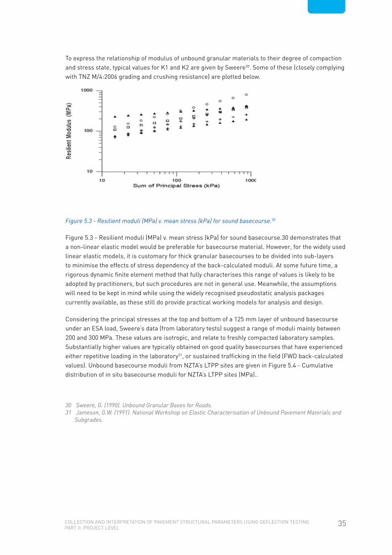
To express the relationship of modulus of unbound granular materials to their degree of compaction and stress state, typical values for K1 and K2 are given by Sweere30. Some of these (closely complying with TNZ M/4:2006 grading and crushing resistance) are plotted below.

Figure 5.3 - Resilient moduli (MPa) v. mean stress (kPa) for sound basecourse.30

Figure 5.3 - Resilient moduli (MPa) v. mean stress (kPa) for sound basecourse.30 demonstrates that a non-linear elastic model would be preferable for basecourse material. However, for the widely used linear elastic models, it is customary for thick granular basecourses to be divided into sub-layers to minimise the effects of stress dependency of the back-calculated moduli. At some future time, a rigorous dynamic finite element method that fully characterises this range of values is likely to be adopted by practitioners, but such procedures are not in general use. Meanwhile, the assumptions will need to be kept in mind while using the widely recognised pseudostatic analysis packages currently available, as these still do provide practical working models for analysis and design.

Considering the principal stresses at the top and bottom of a 125 mm layer of unbound basecourse under an ESA load, Sweere’s data (from laboratory tests) suggest a range of moduli mainly between 200 and 300 MPa. These values are isotropic, and relate to freshly compacted laboratory samples. Substantially higher values are typically obtained on good quality basecourses that have experienced either repetitive loading in the laboratory31, or sustained trafficking in the field (FWD back-calculated values). Unbound basecourse moduli from NZTA’s LTPP sites are given in Figure 5.4 - Cumulative distribution of in situ basecourse moduli for NZTA’s LTPP sites (MPa)..

30 Sweere, G. (1990). Unbound Granular Bases for Roads.31 Jameson, G.W. (1991). National Workshop on Elastic Characterisation of Unbound Pavement Materials and

Subgrades.


100

90

80

70

60

50

40

30

20

10

0

Basecourse Modulus (MPa)

All NZ National Highway LTPP Sites

Per

cent

age

of s

ampl

es <

x

100 1000 10000 100000

LTPP Sites

Figure 5.4 - Cumulative distribution of in situ basecourse moduli for NZTA’s LTPP sites (MPa).

The LTPP sites include mostly mature unbound granular pavements with multiple chip seal layers, which result in higher moduli (10th percentile of 500 MPa for FWD back-calculated isotropic values) than newly constructed basecourses.

It is important to appreciate that the modulus of any unbound layer is not simply a function of the component material, but is also dependent to a large degree on the stiffness of the underlying material. In a multi-layer system, Heukelom and Foster32 found (using linear elastic analyses) that the ratio of the modulus of an unbound base layer (Ei) to that of the underlying soil (Ei+1) was limited to Ei / Ei+1 < 2.5. Their rationale was that an unbound material cannot be properly compacted on a soft subgrade.

Alternatively, if a stiff dense unbound granular layer overlies a yielding foundation, then horizontal tensile strains will occur and the upper layer will de-compact. Heukelom and Foster supported this practical explanation theoretically, showing that tensile horizontal stresses would tend to be induced at the bottom of layer i if the Ei / Ei+1 ratio exceeded 2.4. Under repeated loading, de-compaction of the overlying unbound layer would occur until its stiffness reduced to a limiting value at which tensile stresses would not occur.

Subsequently, the Shell Pavement Design Manual33 used the concept of modular ratio limitations in successive unbound layers in the relationship:

Ei / Ei+1 = 0.2 hi 0.45 and 2 < Ei / Ei+1 < 4 ( 6 )

where: hi is the thickness (in mm) of the overlying layer.

32 Heukelom, W. & Foster, C.R. (1960). Dynamic Testing of Pavements.33 Shell (1978). Shell Pavement Design Manual: Asphalt Pavements and Overlays for Road.


Subsequently, Brown and Pappin34 found, using more rigorous non-linear finite element analyses, that the above limitations were too restrictive and reported:

1.5 < Ei / Ei+1 < 7.5 ( 7 )

Austroads Design Manual35 requires the granular materials placed directly on the subgrade are sub-layered using, as constraints, sub-layer thicknesses that must be approximately in the range of 50-150 mm and that the ratio of moduli of adjacent sublayers does not exceed two. Moffat & Jameson36 used sub-layering in multi-layer linear elastic models to refine the original AUSTROADS procedures for mechanistic design of new unbound granular pavements, and proposed the following:

§ Divide the granular materials into five layers of equal thickness

§ Adopt the vertical modulus for the top sub-layer from (but not exceeding tabulated upper bounds for the materials):

§ Ev top of base = Ev subgrade x 2(total granular thickness/125) ( 8 )

§ Determine the modular ratio of successive sub-layers from:

§ R = [Ev top of base / Ev subgrade] 1/5 ( 9 )

§ Calculate the modulus of each overlying layer starting with the subgrade of known modulus

The modular ratios implied by Equations 8 and 9 are intended for forward design. However, back-analysed moduli should be checked using the above criteria to ensure a reasonable pavement model has been obtained when carrying out sensitivity analyses of different layer thicknesses. Only unbound layer moduli are treated in this manner, as the moduli of strongly bound materials are influenced much less by the stiffnesses of underlying layers.

5.5.5 relating In situ FWD or laboratory Moduli to CBr and DCP

Most researchers have difficulty in obtaining any consistent correlation between dynamic modulus and CBR for unbound aggregates, e.g. Sweere30.

Figure 5.5 - Laboratory resilient modulus (Mr) versus CBR for unbound basecourses.30

34 Brown, S. F. and Pappin, J. W. (1985) Modelling of Granular Materials in Pavements.35 Austroads (2008-2009). Austroads – Guide to Pavement Technology.36 Moffat, M.A. & Jameson, G.W. (1998). Characterisation of Granular Material and Development of a Subgrade

Strain Criterion.


If the assumption is made for Sweere’s data that (i) there is a linear relationship, and (ii) any correlation should pass through the origin, then the equation would be (very approximately) E = 1 x CBR.

Similar difficulty with correlations has been found for fine grained soils (George & Uddin, 2000):

Figure 5.6 - Laboratory dynamic modulus vs dynamic cone penetration index (and hence CBR) for fine grained subgrades.37

When CBR is estimated by penetrometer, then the variation in predicted modulus is further compounded by a factor of about two, as evidenced by the spread of data obtained when the method was developed38. Some correlation was found in a New Zealand study of recent volcanic subgrade soils, but only after categorising into discrete soil types.

Figure 5.7 - In situ modulus vs in situ CBR for NZ recent volcanic soils.39

37 George, K.P. & W. Uddin.(2000). Subgrade Characterization Study for Highway Pavement Design. 38 Scala A. J (1956). Simple Methods of Flexible Pavement Design Using Cone Penetrometers.39 Bailey, R. & Patrick, J.E. (2001). Determination of the Structural Number of Pavements on Volcanic

Subgrades.


By categorising soil types, local relationships were established for the in situ isotropic dynamic moduli (EISO) of North Island volcanic soils. These are tabled below, along with some of the more traditional equations:

Sandy pumice Bailey & Patrick (2001) EISO = 1 CBR

Silty volcanic soils and brown ash Bailey & Patrick (2001) EISO = 3 CBR

Clayey ash soils Bailey & Patrick (2001) EISO = 10 CBR

Sweere (1990) for coarse granular EISO = 1 CBR

Traditional Limits EISO = 5 to 20 CBR

Austroads anisotropic modulus for subgrades Austroads (2008) Implied Austroads isotropic case (see section 5.4.9)

EANISO = 10 CBR

EISO = 6.7 CBR

Original study for fine grained non-expansive soils using field tests with instrumented vibratory compactor

Heukelom & Klomp (1962) or “Shell”

EISO = 10 CBR

(to a factor of 2)

TRRL LR 1132, Powell, Potter, Mayhew & Nunn (1984) EISO = 17.6 CBR 0.64

NAASRA (1950) CBR<5

CBR>5

EISO = 16.2 CBR 0.7

EISO = 22.4 CBR 0.5

South African Council of Scientific and Industrial Research (CSIR) EISO = 20.7 CBR 0.64

U.S. Army Corps of Engineers. Green & Hall, (1975) EISO = 37 CBR 0.71

EISO = 1 CBR

Table 5.2- Modulus versus CBR Relationships.

It is clear that a local, material specific calibration is required. The generally accepted reason for the level of correlation shown above is that the dynamic modulus is a measure of low strain, rapid, elastic deformation, while the CBR is a high strain, slow, plastic deformation test. The former simulates traffic loading on a pavement, while the latter is more of an index test; therefore there can be little expectation of any consistent correlation.

Furthermore, most cohesive soils have highly stress-dependent moduli, i.e. their stress-strain curves are markedly non-linear as illustrated in Figure 5.2 - Typical subgrade moduli and stress-dependency determined from back-analysis of deflection bowls.. It can be seen on this diagram that the modulus (i.e. slope of the stress-strain curve) for a given cohesive soil evidently varies by a factor of two or three depending on the effective load spread (i.e. depth to the subgrade and stiffnesses of pavement layers). All modulus-CBR correlations for cohesive soils must therefore be defined at a specific applied stress level, and the factors in the above table will increase by up to threefold as the total thickness of granular layers increases from, say, 200 mm to 700mm.

The advantage of deflection testing and mechanistic design is that the dynamic modulus is obtained directy, and at no stage is conversion from modulus to CBR required. This applies to both the design process, and construction verification. The conversion from CBR to modulus is required only when attempting to reconcile destructive test data with deflection analyses. This section highlights the importance of establishing local correlations that include material type and pavement thickness

(applied stress), rather than assuming a nominal factor of 10.

For unbound granular basecourses, NZTA suggests using the following relationship (an approximation based on observations of moduli determined on basecourses that have a known CBR of at least 80) to estimate the CBR of an unbound granular basecourse material:

Ev (MPa) = 5 CBR with anisotropy Ev/Eh = 2 ( 10 )

where Ev and Eh are the vertical and horizontal moduli respectively.

The equivalent relationship for an isotropic basecourse is approximately:

Eisotropic (MPa) = 4 CBR for Ev/Eh = 1 ( 11 )

Sweere30 presents data which are consistent with the above relationships (to within a factor of two) provided the applied stresses (sum of principal stresses) are about 750 kPa. However, the constant of proportionality in the above equations decreases by a factor of four as the applied stresses reduce to 50 kPa. For sands (e.g. subbase materials), the constant of proportionality was found to be about three to four times higher than for gravels. Therefore, the above equations should apply (very approximately) for either basecourses close to the wheel load, or sandy subbase at depth.

Moduli for unbound granular materials are clearly very sensitive to test conditions, requiring close replication of in-service density, water content, grading, applied stresses and underlying support for meaningful measurement of modulus or correlation with CBR.

The large variation is shown graphically below, to highlight the issues addressed in this section.


Figure 5.8 – Published dynamic modulus - CBR relationships.

The above chart provides a significant illustration of the precision and level of reliance that can be placed on any modulus-CBR relationship that is not calibrated for a specific material type and associated environment, applied stress and confinement. This is the principal reason why in situ moduli from deflection tests frequently cannot be reconciled with DCP or in situ CBR results.

However, in practice, pavement design can still be carried out reliably when using either of the more common methods (DCP or FWD) individually, and it is seldom essential to correlate between them anyway.

5.5.6 Moduli of Stabilised Basecourses in New Zealand

Moduli of cement or bitumen stabilised basecourses that have sufficent cement to constitute a bound layer are considered to be less dependent on the modulus of the underlying layer. However, various limitations are applied to the maximum modular ratio that should be used in design.

Because stabilisation in New Zealand is not always comparable with that in Australia or South Africa, specific moduli and modular ratios obtained in an ongoing study (FWD tests have been collected on many recently constructed pavements, mostly in the North Island, for an NZTA research project40) are summarised below. These findings are interim only.

40 Gray et al. (2011). Characterisation and Use of Stabilised Basecourse Materials in Transport Projects in New Zealand.


100

90

80

70

60

50

40

30

20

10

0

Basecourse Modulus (MPa)

All NZ Stabilisation Sites

Perc

enta

ge o

f sam

ples

< x

100 1000 10000 100000

Cement Stabilised

Foamed Bitumen Stabilised

Figure 5.9 - Cumulative plot of basecourse modulus for all New Zealand cement and foamed bitumen stabilisation study sites.

The reason for the wider range of cement stabilised moduli, is that while many of the sites are intended to be only modified (so that the basecourse does not become bound and susceptible to cracking), there are also sites with higher cement contents which may be pre-cracked, or intentionally bound. Note the majority of the stabilised sites are relatively young; for mature sites, the 10th percentile will increase and the 90th percentile will reduce.

5.5.7 Seasonal effects

The back analysis of a deflection bowl provides results for the specific water content at the time of testing. Seasonal variations in moduli must therefore be considered before calculating residual life and overlay requirements. Software packages vary in the way seasonal effects are incorporated. One option is to increase deflections by a multiplier in the range of 1.1 to 1.6 if measurements are not taken during a wet period. Another approach is to assume an annual sinusoidal variation in moduli between a maximum and minimum value (usually, the subgrade modulus alone would be varied but the factor could be applied to all unbound layers, with a similar outcome).

In a long-term study of deflection changes with seasons in Australia, Rallings & Chowdhury41 found a generally sinusoidal variation in peak deflection each year, and concluded that a seasonal adjustment factor of 1.1 would be appropriate for deflection measurements made between mid-summer and the end of autumn. The data they obtained include both “wet” and “dry” rainfall areas; there is clearly more seasonal deflection fluctuation in dry areas. If the design condition for the subgrade were taken towards the wetter state rather than at the median condition, then an adjustment factor of about 1.3 would be indicated by the data.

41 Rallings R. & Chowdhury, F. (1995). Seasonal Variations in Pavement Deflections.


Another similar study undertaken at Delft University42 produced comparable sinusoidal seasonal fluctuations in subgrade moduli from FWD measurements taken over a two-year period, but no specific guidelines for generally assessing seasonal effects were indicated.

A considerable degree of judgment will be required to assess seasonal adjustment factors for specific sites. Factors listed in Table 5.3 - Seasonal adjustment factors for deflection testing (after Rallings & Chowdhury41& van de Pol et al42). are suggested as provisional guides for temperate climates, such as New Zealand. This table draws on the above references and is supported by studies in progress. The subgrade water content at the time of testing should be assessed relative to expected ranges in that locality.

subGraDe conDiTion aT TiMe oF TesTinG

Mean Annual Rainfall * Very wet Wet Dry Very dry

500 mm 0.95 1 1.15 1.3

1000 mm 0.95 1 1.1 1.2

* interpolate or extrapolate in proximity

Table 5.3 - Seasonal adjustment factors for deflection testing (after Rallings & Chowdhury41& van de Pol et al42).

5.5.8 layer Thickness Sensitivity

The Odemark43 method primarily considers the stiffness of the various layers rather than moduli directly, i.e. for isotropic layer moduli (E), the overall layer stiffness is proportional to:

h3 E/(1-µ2) ( 12 )

where h is the layer thickness and µ is Poisson’s ratio.

Therefore, when back-analysing to find the layer modulus E from an assumed layer thickness h, a small error in layer thickness will translate to a large error in modulus. The same sensitivity occurs in the other analysis methods that use numerical integration (e.g. CIRCLY). The expression is relatively invariant to the ranges of Poisson’s ratio μ found in practice.

However, it is important to consider only the approximate magnitude of basecourse and subbase layer moduli (as any one interval of “uniform” road will exhibit a wide range of moduli within each layer). Results should not be regarded as precise. This comment does not apply to subgrade moduli, as these values are determined explicitly and results will generally be more reliable, provided any non-linearity of the modulus is taken into account.

Also in the later stage (when determining overlay requirements), it is effectively the layer stiffness (given by the product of the layer thickness and the cube of its modulus) rather than the layer modulus which is used in the calculation, and hence when assessing subgrade strains, the design overlay thickness is affected minimally by reasonable assumptions regarding layer thicknesses.

42 Van de Pol et al. (1991). Seasonal Variations of Subgrade Response.43 An approximate method of calculating stresses and strains in multiplayer pavement systems by

transforming this structure into an equivalent one-layer system with equivalent thicknesses but one elastic modulus.


5.5.9 rigid Base Condition

An apparently non-linear subgrade modulus (or linear elastic sub-layers becoming stiffer with depth) could be incorrectly inferred from the composite modulus plot because of a very stiff layer located at depth. For this reason, noting any outcrops and regional geology is important. If rock is present within about 3 m of the pavement surface, an “infinitely stiff” boundary must be used in the model. If this is not done, overlay results can be speculative. Some software packages provide options for computing the depth to a rigid base automatically from the response of the outer geophones (e.g. ELMOD).

5.5.10 anisotropy

Austroads44 suggests that unbound pavement materials may be anisotropic (i.e. they have a vertical to horizontal modular ratio, Ev/Eh, that may be greater than 1). In particular, a degree of anisotropy of 2 is used for design of unbound granular materials and subgrade layers45. Bound granular materials, on the other hand, are considered isotropic, i.e. they are assigned a degree of anisotropy of 1.

However, other than CIRCLY and FLEA, very few software packages use anisotropy. Furthermore, there is substantial worldwide experience founded on analyses that assume only isotropic conditions for all material types.

To ensure the comparative results from software programs using isotropic moduli and those using anisotropy are valid, it is necessary to determine the applicable modulus constant (Ki-a) in the relationship:

Ev,n=1 = Ki-a * Ev,n=2 ( 13 )

Where: Ev,n is the vertical modulus with modular ratio of n.

Logically, it would be expected that the equivalent isotropic modulus (E v,n=1) for a material with modular ratio n =Ev/Eh=2 must be somewhere between the extremes,

i.e. 0.5 < Ki-a < 1 ( 14 )

Ullidtz46 gives the analytical solutions for anisotropy. The comparison between pavement structures which are anisotropic and their isotropic equivalents cannot be determined directly; however, Ullidtz’s equations can be solved iteratively to provide the theoretical relationships. The constant Ki-a is found to be independent of stress, but is very slightly dependent on the depth below the surface, Poisson’s ratio, and the loaded area. The relevant values for highway situations beneath a 1 ESA load range from about 0.67 to 0.75 for anisotropy of 2.

For subgrade material (at a depth of say 0.3 to 0.5 m or more, and Poisson’s ratio of 0.45), a value of 0.67 to 0.85 for Ki-a provides a practical equivalent, i.e. a subgrade with anisotropic modulus (Ev,n=2 = 100 MPa) could be modelled as a material with an isotropic modulus of approximately 67 to 85 MPa.

For basecourse material (say 100 to 150 mm thick with Poisson’s ratio of 0.35), Ki-a will be about 0.70 to 0.85. A typical M/4 modulus of about Ev,n=2 = 500 MPa is equivalent to a material with isotropic modulus of 350 MPa.

44 Austroads – Guide to Pavement Technology (2008-2009) Part 2, Table 6.3.45 Austroads – Guide to Pavement Technology (2008-2009) Part 5 ,Section E.3.3.46 Ullidtz, Per (1987). Pavement Analysis. Table 3.2.


However, recent trials using the FLEA program suggest generally higher factors closer to 0.85, rather than 0.7. This would suggest a typical isotropic basecourse modulus of about 425 MPa.

Figure 5.4 - Cumulative distribution of in situ basecourse moduli for NZTA’s LTPP sites (MPa). shows the cumulative distribution of isotropic basecourse moduli determined from FWD testing on unbound granular basecourses in NZTA’s LTPP sites. This shows a 10 percentile value of 500 MPa.

Note again that the issue does not arise with cemented (bound) materials or asphalt; Austroads indicates isotropic moduli (a degree of anisotropy of 1) should be used for these materials.

The majority of software packages for back-analysing FWD deflection bowls10 assume isotropic moduli for all layers. The practical reason for this is that only vertical deflections are measured with commonly available equipment. The horizontal moduli (transverse and along the wheelpath) and horizontal components of Poisson’s ratio are usually unknown and cannot be readily determined.

Little information is presented in the Austroads Guide on sensitivity of analyses to anisotropy. Anisotropy remains as one factor in the stiffness expression that is determined by the back-analyses and cannot be deduced explicitly. The rationale for assuming a lower horizontal modulus may be because unbound granular materials will generally not be able to withstand tension, yet most layered elastic software packages assume a constant modulus so that negative stresses will develop with any negative strain. Negative strains might conceivably be modelled with less error by assuming large anisotropy: for a value of 10, Ki-a would be about 0.45. In the anisotropic model, it is still necessary to assume three other variables (Poisson’s ratio and layer thickness as well as modular ratio), to determine in-situ vertical modulus.

Adding variable anisotropy capability has been considered for a future ELMOD upgrade, but is not receiving high priority. Ullidtz (pers. comm.) comments:

» “Including anisotropy would introduce one more unknown parameter, and a parameter that is very difficult to measure, but it would be uncertain whether this would bring you closer to or further away from the actual stresses and strains in the pavement.”

The anisotropy Austroads uses has significant implications with regard to allowable subgrade strains, because the relationships resulting are:

Ev = 10 CBR, Eh = 5 CBR ( 15 ) (because modular anisotropy of 2 is adopted).

Therefore, from the discussion on anisotropy (Section 6.4.8), the equivalent isotropic subgrade modulus is:

E isotropic = 7 CBR (rather than 10 CBR) ( 16 )

This assumes the subgrade is at a depth of about 300 mm and has a Poisson’s Ratio of 0.45, although there is very little sensitivity to these parameters. Equations 15 and 16 clearly differ from relationships for estimating the subgrade modulus from CBR that most organisations around the world have adopted.


The same applies with regard to the Austroads perspective on modulus anisotropy. The compensating consequence of these differences is that the Austroads subgrade strain criterion (derived by back-analysing subgrade CBR design curves) appears considerably more optimistic than subgrade strain criteria recognised by other organisations, as can be seen by its distinctive separation in Figure 5.10 below.

Figure 5.10 – Subgrade Strain Criteria.


6. rehabilitation Treatment: Mechanistic Design

6.1 GeneraLAfter completing the deflection bowl back-analysis and determining layer moduli, rehabilitation options should be evaluated (preferably with the same software used for forward-analysis). Suitable treatments can be modelled, and checks made to confirm that strains within all layers are acceptable for the number of ESA loadings intended in the design life. Using the Austroads recommended general mechanistic procedure (GMP), the compressive vertical strains induced by a 1 ESA loading at the top of the subgrade and the horizontal tensile strains at the bottom of any bound layers are computed and compared with empirical allowable strains for the design traffic.

Some organisations also specify fatigue criteria for unbound granular layers.15 These are typically based on allowable vertical stresses or strains at specified depths, and include limits based on either repeated load triaxial (RLT) testing or in situ tests. RLT and FWD are seen as complimentary tests; the RLT can quickly explore the effects of a regional variation from a standard basecourse, while the FWD provides a field check on factors such as in situ stress, delays between loading cycles and environmental impacts.

Given that the in situ FWD testing on a mature pavement should be on materials that are appropriately conditioned, three of the more relevant parameters to consider when assessing basecourse life are:

§ The quality of aggregate within each layer

§ The basal support provided to that layer

§ The thickness of the layer

Deflection testing on New Zealand’s LTPP sites and case histories from pavements with unbound basecourses exhibiting severe distress have been used to establish a dual criterion which addresses the first two factors:

§ the vertical compressive strain at the centre of the layer will be directly related to the modulus of the aggregate; therefore it is used to characterise aggregate quality

§ the horizontal tensile strain at the base of the layer is used to characterise the effectiveness of the support provided by the underlying layer(s)

This model is undergoing continual development as relevant field test data is collected.


6.2 MechanisTic DiaGnosis oF PaveMenT DisTressVisual assessments are the primary means of assessing distress. However, where there has been recent surfacing maintenance, deflection testing is often a cost effective means of diagnosing potential distress modes and residual life (as described in Part 1 of this Guide).

If the distress is visually apparent but the precise origin uncertain, comprehensive diagnosis can be carried out by having an observer on site to direct the FWD operator. The aim is to ensure the load plate and geophone spread is located entirely within identified segments of wheelpath distress where the severity is relatively uniform over the length of the spread (1.5 m). The observer then logs the exact distress at the test point. Testing is not necessarily carried out at uniform spacing, instead it is carried out selectively to encompass all distressed segments and a selection of undistressed segments. The severity and mode of distress are both logged at each of the FWD test points. The modes are appropriate to the forms of distress, and the severity is a numeric code as per Table 6.1.

sTrucTuraL DisTress MoDe

severiTy severiTy coDe

Rutting None 0

Cracking Initial 1

Pumping Advanced 2

Shoving Severe 3

Patching Terminal 4

Table 6.1 – Distress logging codes.

It is preferable to have just one person logging, as it is the relative severity that is important in the subsequent analysis. Where practical, rutting is usually measured quantitatively by the observer using a 2 m straight edge and wedge immediately behind the load plate.

After processing, the data can then be interrogated using diagnostic comparisons. For example this could involve plotting the severity of either cracking or shoving distress against basecourse parameters (such as modulus), then trying other parameters relating to the intermediate layers or the subbase to discern which layer provides any correlation. Plotting the subgrade modulus exponent versus rutting or cracking severity will sometimes provide an indication of whether subsoil drainage is a problem. Rutting can be plotted against the modulus of each layer or subgrade to discover whether any one layer is contributing to deformation more than the others.

If there are suitable as-builts, then rutting depth versus pavement depth would confirm whether the pavement depth is significant. In this way, causes can be distinguished between, for example, a construction fault (i.e. degree of compaction of a granular layer), versus an engineering issue with a subgrade for which the stiffness has been over-estimated with consequent under-design of the pavement thickness. Similar distinctions can be made by examining the measured modular ratios with respect to Austroads standard values.


6.3 unbounD GranuLar PaveMenT rehabiLiTaTionThe New Zealand Supplements to the Austroads Guide promote mechanistic methods for rehabilitating all pavement types to make use of the existing pavements’ measured properties. However for new full depth unbound granular pavements (including widening), only the subgrade properties can be measured in situ. This is why the traditional CBR thickness design method is recommended. Design CBR should consider values exhibited by nearby established pavements on similar terrain wherever practicable.

A fundamental improvement to the mechanistic design of rehabilitation treatments is the use of precedent strain analysis to assess the most appropriate strain criterion for a given situation. This “precedent performance” design process has been used in New Zealand using the same fundamental concept since the 1970s. NZTA strongly promotes it as the primary design method for rehabilitation treatments, provided the terminal distress mode is the result of subgrade strain. The New Zealand Supplement precedent method requires substantial adaption before it can be used to evaluate pavement designs where either chip seal cracking or shallow shear (shoving) is the dominant distress mode.

The back-calculated strains from deflection testing are ideal for applying the precedent strain method. There are two alternatives given in the Supplement47, but when there is thorough FWD data, it is important to use the Supplement’s Equation 10.4 as this gives the more efficient and reliable design.

The two components of the current New Zealand Supplement (one for new pavements and one for rehabilitation) are currently being revised. Nevertheless, the precedent performance method using deflection testing is likely to remain the preferred method for rehabilitation design where it is applicable. The reasons for this are:

§ It implicitly takes full account of the long term average support the subgrade provides – i.e. it is relatively insensitive to the season in which the rehabilitation section happens to be tested.

§ It is insensitive to the absolute value of measured traffic and assumption of ESA’s per heavy for a particular route, as it depends only on that route’s long term growth.

§ It acknowledges the inherent variability of natural materials and does not require that all subgrades will necessarily follow the same strain criterion as determined by Austroads from Australian experience. In practice, the allowable strain on some New Zealand subgrades (particularly recent unweathered volcanic ashes) in the central North Island may be 1.5-2.0 times higher.

The method also has important limitations that must be taken into account - these are likely to be included in the next upgrade to the Supplement.

47 Transit New Zealand, TNZ (2000). New Zealand Supplement to the Austroads Pavement Design Guide.


6.4 basecourse sTabiLisaTion On the basis of the typical moduli for cement stabilised basecourses given in Figure 5.9 - Cumulative plot of basecourse modulus for all New Zealand cement and foamed bitumen stabilisation study sites., a 10th percentile design isotropic modulus of 400 MPa might be envisaged for stabilised basecourses. However, design moduli of 2000 or 5000 MPa are sometimes specified. NZTA classifies stabilised basecourse moduli of up to 1500 MPa as modified with similar design characteristics (anisotropic moduli and Poisson’s ratio of 0.35) as for unbound aggregates. Between 1500 MPa and 5000 MPa is regarded as lightly bound, while over 5000 MPa is heavily bound. All cement bound materials (whether intact or cracked) are regarded as isotropic with Poisson’s ratio of 0.2).

For foamed bitumen stabilisation, the NZTA Supplement to the Austroads Guide gives recommendations of 800 MPa anisotropic modulus with Poisson’s ratio of 0.3 and no sublayering. The typical New Zealand cement content is 1.0 to 1.5% with 2.7 to 3.0% foamed bitumen.

There is little published information showing how the in situ moduli of stabilised layers relate (if at all) to the modulus of the underlying layer. Relevant parameters from all New Zealand stabilisation study sites are given below (note these use isotropic moduli in all cases, because in situ anisotropy cannot be deduced from any simple low cost test such as the FWD).

Figure 6.1 - Stabilised layer modulus (MPa) vs standard central deflections (mm) for all New Zealand cement stabilisation study sites.


Figure 6.2 - Stabilised layer modulus (MPa) vs standard central deflections (mm) for all New Zealand foamed bitumen stabilisation study sites.

Both material types show moduli that apparently decrease as the standard central deflection increases. These are not independent variables because clearly any layer with intrinsically good stiffness will provide better loadspread and hence produce less deflection. Simplistically however, a line can be drawn through the lower 5th-10th percentile of the data set to generate an equation that will define a “characteristic” design modulus for various support conditions. This indicates what should be readily achievable in practice. Designers can work through an iterative process (such as the following) using any layered elastic mechanistic design program:

§ Adopt an initial pavement profile using Austroads sublayering for unbound granular aggregates for the given subgrade modulus, setting the thickness of the top layer equal to the local preference for stabilised layer depth (typically 200 mm)

§ Calculate the standard central deflection (under a 40 kN FWD load) using layered elastic theory

§ Read off the expected characteristic design modulus from the above figure (or equations shown there, but not exceeding NZTA New Zealand Supplement limits)

§ Substitute the FBS design modulus into the pavement model, optimise layer thicknesses (and consequent moduli) for a minimum cost design, iterating as required to obtain satisfactory cumulative damage factors in the usual way.

More rigorous means for designing pavements that are stabilised (bound and modified, cement or FBS) based on the in situ testing results from the New Zealand stabilisation study sites have been documented48. As the procedure involves a number of steps, these have been automated into a mechanistic design spreadsheet. Note: the stabilisation not only reduces subgrade strains, but also minimises permanent deformation in the stabilised layer itself where appropriate mix design has been carried out.

48 von Pein et al. (in prep). Characterisation of Stabilised Basecourse Materials.


6.5 PresenTaTionSoftware packages produce a range of display outputs, but most include options that can be transported into spreadsheets and graphed to suit individual project requirements.

Spreadsheet files of FWD information can be readily supplied electronically and viewed graphically. Graphical reports can show the inferred moduli and relevant parameters against the overlay requirements or depth of basecourse stabilisation using the mechanistic procedures described in the New Zealand Supplement. It is generally useful to compare the overlay design methods using both the Austroads subgrade strain criterion and the NZTA precedent strain criterion.

The visual condition assessment and known performance of local materials must then be used to check the appropriateness of the preliminary analytical model. Any inconsistencies must be addressed, the layer thicknesses adjusted according to the destructive test information, and a final model developed.

An example of a final report presentation of parameters is provided below in Figure 6.3 - Pavement structural analysis from state highway section FWD survey.. This shows a number of parameters plotted against road chainage. Working from the top down, these parameters are:

§ The overlay thickness required (assuming that there is no level constraint, and the appropriate overlay design method has been selected, e.g. Austroads Simplified, Austroads GMP, or New Zealand Supplement).

§ The depth of stabilisation of the existing basecourse with cement or FBS, if that option were to be considered, using the New Zealand Supplement tensile strain criterion.

§ The remaining life of the pavement model using the strain criteria applicable for the selected overlay method, and the traffic since construction.

§ The calculated moduli for each of the test points back-analysed from the pavement deflection bowls. Colour coding enables the various layers to be readily identified.

§ The ESA (in millions) that the pavement is expected to endure over its design life.

§ The critical layer; the layer that governs the pavement’s design life according to the adopted strain criterion.

§ The adjusted structural number (SNP).

§ The subgrade strain ratio, which is defined as the calculated subgrade strain divided by the allowable subgrade strain. Values greater than 1 indicate that the subgrade strain is greater than that required to meet the design life.

§ The subgrade modulus non-linearity exponent, which enables the likely soil type to be identified in the subgrade (as per the previous discussion in this report) and points to poor subsurface drainage when it could be a factor.

§ The normalised modular ratio.

§ The normalised curvature, defined as the ratio of the measured curvature to the allowable curvature from Austroads.

§ the actual dynamic deflections (corrected to standard temperature for an eight tonne equivalent design axle loading).

§ the layer thicknesses used in the model.

To analyse sensitivity to layer thicknesses, separate back-analyses are required. This will allow variations in ESA, overlay modulus or thickness, alternative strain criteria, and basecourse stabilisation to be considered.


When a satisfactory model is developed, the individual results should be grouped into structurally uniform sub-sections, showing the practical intervals for individual forms of treatment specified for construction. This vital step ensures a cost-effective approach, ensuring the design life is achieved without superfluous overlay. The emphasis is placed on obtaining comprehensive in-situ test data so structurally deficient sections can be clearly delineated from areas requiring no strengthening. This avoids the over-design that can result where a single form of treatment is applied to an extended length of pavement.

Figure 6.3 - Pavement structural analysis from state highway section FWD survey.


The above example was taken from a road in which shallow shear was the principal distress mode. In this case, the Austroads strain criterion would normally be adopted for the subgrade, as the precedent subgrade strain method would tend to be over-conservative. Safeguarding against future shallow shear would be the principal design consideration. Further documentation about this this issue is being prepared.

Although the ELMOD software was used in this instance, EFROMD2 together with CIRCLY will produce the same set of parameters except for the subgrade modulus exponent (n). Limitations of the various analysis methods are given in Section 2.3 of this report.

The above road could be interpreted in distinct subsections, as shown in the following table.

chainaGe Layer 1 MoDuLus n subGraDe MoDuLus

ssr* criTicaL Layer

overLay (MM)

FroM To MeDian 10%iLe MeDian MeDian 10%iLe MeDian

0.010 0.163 952 662 -0.3 91 54 0.73 5 0

0.163 0.488 504 334 -0.4 58 34 1.22 5 80

0.488 0.823 772 371 -0.3 84 61 0.82 5 0

0.823 1.410 505 327 -0.4 52 29 1.38 5 100

1.410 2.263 1008 681 -0.3 64 20 0.81 5 0

2.263 2.763 561 373 -0.8 21 12 1.26 5 80

2.763 2.913 417 194 -1.1 22 7 1.95 5 180

2.913 2.963 279 279 -2.5 4 4 9.65 5 570

2.963 3.100 537 383 -0.7 19 12 1.33 5 80

* Subgrade Strain Ratio – values less than 1 indicate that calculated strains are less than the allowable strain.

Table 6.2 - Sub sectioning for uniform intervals of the road analysed for Figure 6.3 - Pavement structural analysis from state highway section FWD survey. (above).

Section 1 - shows relatively high basecourse and subgrade moduli. No surface distress was apparent. The subgrade strain ratio is much less than one, i.e. strains are already much lower than required by Austroads and hence no overlay is required.

Sections 2 & 4 - show much greater variability in the basecourse moduli; including some very low values. Layer 1 is shown to be critical, i.e. the analysis indicates that in several places the basecourse will be experiencing higher strains than in the subgrade: there would be clear potential for shallow shear. (The latter was markedly evident from visual survey). Using the Austroads strain criterion an overlay of 100 mm of unbound basecourse is required.

Sections 3 & 5 - show only minor structural deficiency and it is evident that the basecourse modulus is uniformly high. No structural overlay is needed. Apart from several localised points, the subgrade strain ratios are slightly less than one, i.e. marginally less than required. (For new pavements, a


subgrade strain ratio much less than one gives a measure of the over-design incorporated.)

Sections 6-9 - indicates that the subgrade CBRs are lower than elsewhere on the site and the basecourse moduli are also poor and highly variable – especially at the two points in section 8. The greatest strains are occurring in the subgrade in part and in the basecourse for the remainder, (critical layers are 1 and 4). The subgrade modulus non-linearity exponent, n, is unusually low (i.e. highly non-linear), suggesting that the potential for improving subsurface drainage should be checked here.

Where precedent subgrade strain information is required, the appropriate strain ratio can be selected from the graph (Figure 6.3 - Pavement structural analysis from state highway section FWD survey.) for any subsection, and the actual precedent strains calculated directly from the Austroads subgrade strain relationship.

6.6 DesiGn revieWAt completion of deflection testing and visual assessment, the designer should review all raw data and the preliminary interpretation in order to assess the need for (and locations of) destructive testing (e.g. coring, test pits, or penetration tests).

In Figure 6.3 - Pavement structural analysis from state highway section FWD survey. and Table 6.2 - Sub sectioning for uniform intervals of the road analysed for Figure 6.3 - Pavement structural analysis from state highway section FWD survey. (above)., where shallow shear was evidently the principal distress mode, the test points showing the lowest basecourse moduli (or where basecourse strains are higher than subgrade strains) should be selected for test pitting and CBR testing. This should follow the guidance in Section 10.3 of the New Zealand Supplement. A test pit at approximately chainage 1.000 would identify the weakest basecourse and confirm the typical subgrade stiffness for the first three sub-sections.

For sub-section four, basecourse quality should be investigated around chainage 2.750. However, care is needed to identify the more adverse areas visually as the results show marked fluctuation in stiffnesses. The subgrade CBR here could be significantly lower than at the first test pit site at chainage 1.000.

Re-analyses for final design are normally undertaken to incorporate destructive testing information. Geometric constraints need to be considered (for example kerb and drain levels) and then comparisons may be made to determine the most cost effective treatment. These could include, for example, local digouts, overlay, cement stabilisation or reconstruction. In this example, costs for overlays of 100 to 120 mm of M/4 are compared with those for cement stabilisation of about 250 mm to give the same design life. However, the example shows some points where very deep stabilisation would be required, and where the subgrade may be too weak for this option.


7. Mechanistic Design: new Pavements

7.1 unbounD GranuLar PaveMenTsEmpirical chart design is the standard method for unbound granular pavements where design is usually based on soaked CBR samples. In some cases (such as widening design, or where a new road is being constructed on the same subgrade in close proximity to other roads), deflection testing can be used to assess an applicable subgrade modulus for mechanistic design.

A question commonly arising in these situations is “how many tests are necessary to define an appropriately conservative design value for a given homogeneous treatment length?” The design value, or “characteristic” value for each treatment length, is generally taken as the 10th percentile. This is a commonly adopted reliability level for highways (Austroads49). Note: the 5th percentile has been implied in some New Zealand contracts, while higher percentile values may be appropriate for arid climates, or roads of lesser importance.

The advantage of non-destructive testing (e.g. FWD) is that the method allows a large number of values to be obtained quickly for each treatment length, whereas if field CBR tests (or Scala Penetrometer approximations) are utilised, then the number of tests per treatment length will often be as low as three. Conducting fewer than 10 tests will affect the 10th percentile design value assessment, as even the lowest value may be an over-optimistic (unconservative) estimate of the characteristic value. Attempting to determine a 10th percentile based on normal (Gaussian) distribution is therefore often invalid. (CBR and modulus often tend to be skewed distributions, and are commonly log-normal rather than normal.)

To address this issue, studies were undertaken in several New Zealand regions to obtain large numbers of tests in many treatment lengths. The objective was to assess the typical range of subgrade support within each treatment length. The results for cumulative distributions of CBR (inferred from FWD moduli) from each treatment length in one of the regions studied is shown below:

49 Austroads Guide to Pavement Technology (2008-2009). Part 2 Section 5.5


Figure 7.1 - Distribution of CBR values per treatment length in one New Zealand region.

Notably, the curves have generally similar total ranges and distributions. The modulus and CBR have approximately similar distributions (irrespective of what correlation may be argued for each region or treatment length). Therefore, these data can be used to propose a simplistic guideline for establishing characteristic subgrade support values where there are fewer than 10 tests (either CBR, DCP or FWD) per treatment length.

The approach suggested from inspecting the cumulative distributions is as follows. Each characteristic value should be able to be reasonably approximated as a constant factor (C10%) multiplied by the median value from that treatment length, e.g.:

CBR Design = C10% x CBR Median ( 17 )

where C10% is the appropriate factor to reduce the median value to the 10th percentile value in that region. The same factor applies to determine the 10th percentile modulus direction from limited FWD results.

The New Zealand study has so far been limited to only three regions, but many treatment lengths in each region have been included giving the following values.

reGion 5Th PercenTiLe FacTor

(c5% )

10Th PercenTiLe FacTor

(c10% )

Auckland 0.58 0.61

Wellington 0.58 0.65

Taranaki and Wanganui 0.63 0.70

Table 7.1 - Median to percentile reduction factors for subgrade support value.


The results do not differ too widely between this limited number of regions. Interim values for any New Zealand region seem to be about 0.6 and 0.65 for C5% and C10% respectively.

In practice, when budget for site investigation limits the number of non-destructive test points to less than 10, applying this method would entail:

§ Determining the median stiffness value from a minimum of three test results, preferably five or more. (Note: if they are in situ tests, the Austroads Guide indicates they should be done at a time of year when soil water content is relatively adverse.) The in situ tests may be CBR, DCP or FWD/LWD if the subgrade is exposed. Laboratory testing (soaked CBR) will be the only option if in situ testing cannot be carried out when the subgrade is significantly drier than its design condition (usually late winter/early spring).

§ Evaluating which percentile is warranted (depending on the region and the road’s importance level), or if unclear simply adopt C10% = 0.65.

§ Calculating the characteristic design subgrade stiffness from the product of the reduction factor and the median stiffness.

The resulting design should enable more reliable and systematic design for small projects where funding for comprehensive site investigation is not always available. It will also make it more likely that post-construction deflection testing for verifying design life will relate to the parameters adopted for design.

7.2 PaveMenTs WiTh MuLTiPLe bounD LayersIn these cases, mechanistic design to standard Austroads principles can allow innovative design of a large variety of permutations. An efficient means of assessing the design CBR is given in section 7.1. The concepts are covered comprehensively in the Austroads Guide and New Zealand Supplement. For new stabilised layers, information from FWD studies on New Zealand pavements is given in section 6.3.


8. construction Quality assurance and Design Life verification

8.1 PreDicTinG DesiGn LiFe The future performance (expected life) of a new or rehabilitated pavement is most practically verified by non-destructive methods (e.g. deflection tests), in conjunction with as-built information. NZTA’s requirement is typically that 90 to 95% of the pavement should not reach a terminal condition until it has been in use for at least 25 years. Specific test requirements have been established for NZTA’s Performance Based Rehabilitation Contracts.50 A readily appreciated way of demonstrating life is with cumulative distribution curves for pavement parameters, and noting the relevant percentile values.

Until recently, the only measure in common use was to determine if the standard central deflection complied with the empirical Austroads allowable values for unbound granular pavements. However, because each potential distress mechanism is not considered, the reliability of the prediction is limited. For bound layers, curvature of the bowl would also be considered, but the thickness of the bound layer is also significant.

Mechanistic analysis provides a much more fundamental approach when a check of future pavement life can be made for each of the various structural distress modes (rutting, roughness, flexure, cracking and shoving). Austroads’ most basic approach is to check at least rutting (from vertical compressive strain at the top of the subgrade) and cracking of any bound layer (from horizontal tensile strain at the base of that layer).

The life prediction process can be applied to new full depth constructions or newly rehabilitated pavements. Ideally, quality assurance testing should be completed after bedding in (i.e. traffic of at least 10,000 ESA should be applied), but before surfacing so that any necessary intervention can be completed. Another application for life prediction is when assurance is sought for a minimum life expected before the need for any structural maintenance prior to a change of ownership of an existing road.

NZTA50 recommends FWD testing is carried out at least one year after construction to verify the design life of newly constructed pavements. Contractually, prediction accuracy can be an issue. NZTA’s perspective is the information now readily obtainable from deflection testing,

» “poses a challenge for establishing a fair and consistent evaluation method for the assessment of post-construction structural capacity. In this respect, it has to be recognized that the inclusion of a structural assessment in a performance-based contract is a ground-breaking concept and that a learning curve should therefore be anticipated.”

50 NZ Transport Agency (2003). Guidelines for Performance Based Rehabilitation Contracts. Revised Feb 2012.


NZTA’s key questions to be answered by the structural analysis are:

§ “Were the design assumptions generally realised/achieved during construction?”

§ “What is the expected structural capacity of the constructed pavement?”

8.2 aPPLicaTionThe method is applied using the mechanistic principles described in section 5, with appropriate fatigue criteria for each distress mode of interest. For a new pavement, the total life is calculated, while for those with some trafficking already, the remaining life is calculated. In this manner, a test of both under and over-design is available.

A case history of an existing pavement where remaining life had to be determined is shown in Figure 7.1 - Distribution of CBR values per treatment length in one New Zealand region.. As minor distress had developed, the high-speed data for rut depth and roughness were collected and incorporated into the calculation of remaining life. The figures show the remaining pavement life (assuming a 10% cut-off) is predominantly governed by flexure (top down cracking initiation), and given its current condition, the road is assessed to have a remaining life of 0.3 MESA.

If cracking could be controlled by frequent reseals in the problem interval (which is not usually economic), it would be possible to extend the life to over 1 million ESA before both rutting and roughness would become terminal, and rehabilitation becomes necessary. A targeted programme of overlays might also be considered, as this could be used to extend the life for all three primary failure mechanisms.

Figure 8.1 - Pavement life assessment for each distress mode, by chainage and ESA.


Figure 8.2 - Cumulative distribution of remaining life for each distress mode and governing life.

In Figure 8.2, the dashed line shows the “governing” life, i.e. the minimum life from each of the distress modes considered. This graph shows that where more than one mode of distress is critical along any road length, the cumulative distribution of governing life will be lower than in an equivalent case where only one distress mode occurs.

A useful technique in construction QA, particularly for unbound granular pavements, is to determine the modular ratio of successive layers and compare these with Austroads expectations. In the following case histories, the measured modular ratio at each test point is compared with the ratio expected by Austroads. The resulting ratio is plotted as the normalised modular ratio – i.e. values of at least 1 are as expected while those less than one provide a clear indicator that compaction is likely to be inadequate. Typical results from two satisfactory pavements are given in Figure 8.3.


Figure 8.3 - Cumulative normalised modular ratio distributions for newly trafficked pavements.

The cases shown in Figure 8.3 are from unbound granular pavements where some trafficking has been experienced allowing bedding in of the granular layers. Where only construction compaction has occurred, modular ratios can be expected to be lower. One recent case of a new construction monitored the first compaction attempt on the basecourse.

Figure 8.4 - Increase in normalised modular ratio with additional compaction.


Figure 8.4 shows normalised modular ratios in the range of 0.8 to 0.9. Sealing was deferred and further compaction applied giving a marked increase in modular ratios with only about 10% less than unity. After trafficking, further shakedown would be expected, i.e. it is likely that ratios may increase by 10-30% in the early life of most unbound granular pavements, depending on how well they have been compacted during construction.

Further research on this aspect is in progress, but untrafficked, unbound granular pavements with 10th percentile normalised modular ratios lower than 0.9 may, if already sealed, show some early life rutting due to ongoing densification of the granular layers. The modular ratio, therefore, can serve as an indicator as to whether any deficiency is an issue for the contractor or the designer. The contractor would be responsible if the modular ratios were significantly less than 1.0, (i.e. compaction would be less effective than normally achieved by other contractors). On the other hand, the designer would be responsible if the modular ratios are predominantly greater than 1.0 and the subgrade strain is excessive, (i.e. the designed pavement thickness is inadequate for the 10th percentile subgrade modulus).

If such testing and analysis were undertaken on the subbase layer (or at least on the basecourse prior to sealing), timely intervention can avoid the cost and other issues associated with premature distress. Standard construction should seldom require other than the standard tests in the NZTA B/2 Specification, but where weather conditions have been adverse, or materials appear marginal, or heavy-duty pavements are required, deflection testing can substantially reduce the primary source of risk.

For cement bound or structural asphaltic pavements, the normalised modular ratio still provides an effective quality control measure. It is most readily assessed from FWD testing immediately prior to laying the asphalt or other bound layers.

LiMiTaTions

Structural analysis is not always definitive because in some cases there may be more than one way to interpret the non-destructive data, or it may point to the need for confirmatory intrusive investigation. For this reason, deflection testing alone (while giving a good indication of probable performance) should not be used to conclude unequivocally that the life of a specific pavement would not achieve its design value. Rather, it should be used to flag potential problems that may not yet be evident from visual inspection. (Life in absolute terms will naturally depend on factors other than moduli, principally waterproofing and durability.)

However, in relative terms, structural analysis usually has good reliability, and it will indicate which chainages of the pavement are likely to first experience distress and the probable distress mode that will ultimately result in a terminal condition. Therefore, inspection just before the end of the maintenance period can be focussed on chainages of interest. If there is any distress at the critical chainages, then the model can be readily calibrated for an informed re-evaluation of residual life for the full length of the rehabilitated section.


9. bibliographyAASHO (1961). Interim Guide for the Design of Flexible Pavement Structures.

AASHTO (1986). AASHTO Guide for Design of Pavement Structures. American Association of State Highway and Transportation Officials, Washington.

Austroads (2008-2009). Austroads – Guide to Pavement Technology.

Bailey, R. & Patrick, J.E. (2001). Determination of the Structural Number of Pavements on Volcanic Subgrades. Transfund New Zealand Research Report No. 213, pp 95.

Bretonniere, S. (1963). Etude d’un deflectometre a boulet. Bulletin de Liaison des Laboratorires Routieres, No. 2, Paris.

Browne, A. (2011). 6 Years of Foamed Bitumen Stabilisation in New Zealand – A Performance Review and Comparison to Overseas Practice. 10th Conference on Asphalt Pavements for Southern Africa.

Brown, S.F & Pell, P.S. (1967). An Experimental Investigation of the Stresses, Strains and Deflections in a Layered Pavement Structure Subjected to Dynamic Loads. Proc. 2nd Int. Conf. Structural Design of Asphalt Pavements. Ann Arbor, USA, pp 487 - 504.

Brown, S. F. & Pappin, J. W. (1985). Modelling of Granular Materials in Pavements. Transp. Res. Rec. 1022. Transportation Research Board, Washington, D.C., 45-51.

Dynatest Engineering A/S (1989). ELMOD (Evaluation of Layer Moduli and Overlay Design). Users Manual.

Edwards, P. E. & Fleming, P. F. (2009). LWD Good Practice Guide (Working Draft – under review). Dynatest Engineering, http://www.dynatest.cl/Good%20Practice%20Guide%20-070709-Training%20Day%20Issue.pdf, accessed 20/02/2013.

George, K.P. & W. Uddin.(2000). Subgrade Characterization Study for Highway Pavement Design. Final Report - Sponsored Research Study SS 131, The University of Mississippi, for the Mississippi Department of Transportation, Report No. FHWA/MS-DOT-RD-00-131, December 2000.

Gray, W, Frobel, T, Browne, A, & Salt, G and Stevens, D (2011). Characterisation and Use of Stabilised Basecourse Materials in Transport Projects in New Zealand NZTA Research Report 461.

Green, J.L. & Hall, J.W., Jr. (1975). Nondestructive Vibratory Testing of Airport Pavements. Report No. FAA-RD-73-205, Volume I, NTIS, Washington, D.C.

Heukelom, W. & Foster, C.R. (1960). Dynamic Testing of Pavements. Journal of Structural Division ASCE SM1.

Heukelom, W. & Klomp, A.J.G. (1962). Dynamic Testing as a Means of Controlling Pavement during and after Construction. Proceedings of the 1st International Conference on the Structural Design of Asphalt Pavement. University of Michigan, Ann Arbor, MI.

Jameson, G.W. (1966). Origins of Austroads Design Procedures for Granular Pavements. ARRB Transport Research Report ARR 292.

http://www.dynatest.cl/Good%20Practice%20Guide%20-070709-Training%20Day%20Issue.pdf

http://www.dynatest.cl/Good%20Practice%20Guide%20-070709-Training%20Day%20Issue.pdf


Jameson, G.W. (1991). National Workshop on Elastic Characterisation of Unbound Pavement Materials and Subgrades. Austroads Pavement Research Group Report No. 3. ARRB.

Lytton, R L, (1988). “Backcalculation of Pavement Layer Properties”, Nondestructive Testing of Pavements and Backcalculation of Moduli, ASTM STP 1026, A J Bush III and G Y Baladi, Eds.,ASTM, Philadelphia, pp 7-38.

Moffatt, M. et al (1997). Improved ASMOL Overlay Design Using Falling Weight Deflectometer ARRB Transport Research Ltd WD-R97/011.

Moffat, M.A. & Jameson, G.W. (1998). Characterisation of Granular Material and Development of a Subgrade Strain Criterion. ARRB WD-R98/005. ARRB Transport Research, Australia.

NZ Transport Agency (2003). Guidelines for Performance Based Rehabilitation Contracts. Revised Feb. 2012.

Paterson, W.D.O (1987). Road Deterioration and Maintenance Effects. The Highway Design and Maintenance Standards Series. World Bank. John Hopkins University Press.

Paterson, W.D.O. (1991). Summary Models of Paved Road Deterioration Based on HDM III. Transportation Research Record 1344, pp 99-105.

Powell, W.D., Potter, J.F., Mayhew, H.C., and Nunn, M.E. (1984). The Structural Design of Bituminous Roads. TRRL Report LR 1132, 62pp.Rallings R. & Chowdhury, F. (1995). Seasonal Variations in Pavement Deflections. Road & Transport Research, Vol. 4, No. 1, pp 91-93.

Rohde, GT & Hartman A. (1996) Comparison of Procedures to Determine Structural Number from FWD Deflections. Proc Roads ’96 Conference, New Zealand, pp 99-115.

Salt, G & D Stevens (2002) Modular Ratios for Unbound Granular Pavement Layers. http://www.pavementanalysis.com/index.php?option=com_content&view=article&id=62&Itemid=71

Salt, G & D Stevens (2010). Rationalisation of the Structural Capacity Definition and Quantification of Roads based on Falling Weight Deflectometer Tests.

Scala A. J (1956) Simple Methods of Flexible Pavement Design Using Cone Penetrometers, New Zealand Engineering Journal.

Shabbir Hossain, M. and Apeagyei, A. K. Evaluation of the Lightweight Deflectometer for In-situ Determination of Pavement Layer Moduli. Virginia Transportation Research Council (Virginia Department of Transportation). http://www.virginiadot.org/vtrc/main/online_reports/pdf/10-r6.pdf, accessed 20/02/2013.

Shell (1978), Shell Pavement Design Manual : Asphalt Pavements and Overlays for Road.

Shepard, W.J. (1989). Guidelines for Selection, Design and Construction of Thin Flexible Bituminous Surfacings in New Zealand. Road Research Unit Bulletin 79. N.R.B., Wellington, New Zealand.

Stolle D & Peiravian, F. (1996). Falling Weight Deflectometer Data Interpretation using Dynamic Impedance. Can. J. Civ. Eng. 23:1-8.

Sparks, GH & Potter, DW 1982, An Investigation into the Relationship between California Bearing Ratio and Modulus for Two Clays, Internal Report AIR 295-1, Australian Road Research Board, Vermont South, Vic.

http://www.virginiadot.org/vtrc/main/online_reports/pdf/10-r6.pdf


Sweere, G. (1990). Unbound Granular Bases for Roads. Doctorate Thesis, University of Delft.

Tholen, O., Sharma, J. & Terrel, R.L (1985) Comparison of Falling Weight Deflectometer with other Deflection Testing Devices. Transportation Research Record 1007. Transportation Research Board, Washington, D.C., pp 20 - 26.

Thompson, M.R. & Quentin, L.R. (1976). Resilient Properties of Subgrade Soils, Final Report, Project IHR-063, Illinios Co-Operative Highway and Transportation Research Program, University of Illinois, Chicago.

Tonkin & Taylor (2012). CBR Selection for Pavement Design: Evaluation of characteristic parameters from a small number of subgrade tests. Internal Report.

Transit New Zealand (1989). State Highway Pavement Design and Rehabilitation Manual. National Roads Board, Wellington, New Zealand.

Transit New Zealand, TNZ (2000). New Zealand Supplement to the Austroads Pavement Design Guide.

Ullidtz, Per (1973). En studie af to dybdeasfaltbefaesterlser, Ph.D. Dissertation, The Institute of Roads, Transport and Town Planning, The Technical Institute of Denmark.

Ullidtz, P., (1978). “Computer Simulation of Pavement Performance”, Report No 18, The Institute of Roads, Transport and Town Planning, The Technical University of Denmark, 1989.

Ullidtz, Per (1987). Pavement Analysis. Developments in Civil Engineering 19. Elsevier.

Ullidtz, P. & Coetzee, N.F. (1995). Analytical Procedures in Non-destructive Testing Pavement Evaluation, Transporation Research Record 1482: pp 61-66.

Ullidtz, P. (1998) “Modelling Flexible Pavement Response and Performance”, Polyteknisk Forlag, Lyngby 1998.

Van de Pol, G. J., van Gurp, C.A.P.M., Houben, L.J.M. & Molenaar, A.A.A. (1991). Seasonal Variations of Subgrade Response. Delft University. Faculty of Engineering Report 7-91-203-8.

von Pein, J., Wong, S., Stevens, D., Salt, G.(in prep). Characterisation of Stabilised Basecourse Materials. In Situ Testing and Analyses from New Zealand Highways – Developments Subsequent to NZTA Research Report 461 (& 498).

Wardle L.J. (1980). PROGRAM CIRCLY, A Computer Program for the Analysis of Multiple Complex Circular Loads on Layered Anisotropic Media.

collection and interpretation of pavement structural ... · pavement structural parameters using...

Documents