reactor physics: the diffusion of neutrons - …nuceng.ca/ep4d3/text/3-diffusion-r1.pdfreactor...

Reactor Physics: The Diffusion of Neutrons 1

Reactor Physics: The Diffusion of Neutrons prepared by

Wm. J. Garland, Professor, Department of Engineering Physics, McMaster University, Hamilton, Ontario, Canada

[Based on Chapter 5 of Lamarsh since the treatment there is good]

More about this document Summary:

Neutron movement is modelled herein as a diffusion process. Mono-energetic neutrons are used for illustration purposes. Analytical solutions of the neutron distribution are sought for some simple cases involving fixed sources.

Table of Contents 1 Introduction............................................................................................................................. 3

1.1 Learning Outcomes......................................................................................................... 4 2 Why Diffusion ........................................................................................................................ 5 3 Interaction Rates and Neutron Flux ........................................................................................ 5 4 Neutron Current Density......................................................................................................... 8 5 Equation of Continuity............................................................................................................ 9 6 Fick’s Law ............................................................................................................................ 10

6.1 Derivation ..................................................................................................................... 10 6.2 Validity of Fick’s Law.................................................................................................. 13

7 Question: What about the Conservation of Momentum and Energy? ................................. 15 8 The Diffusion Equation......................................................................................................... 16 9 Boundary Conditions for the Steady State Diffusion Equation............................................ 17

9.1 Boundary Conditions at Surfaces ................................................................................. 17 9.2 Boundary Conditions at an Interface ............................................................................ 18 9.3 Other Conditions........................................................................................................... 18 9.4 Summary of Boundary Conditions ............................................................................... 19

10 Elementary Solutions of the Steady State Diffusion Equation ......................................... 20 10.1 Infinite Planar Source ................................................................................................... 20 10.2 Point Source in an Infinite Medium.............................................................................. 22 10.3 Systems with a Free Surface ......................................................................................... 24 10.4 Multi-region Problems.................................................................................................. 26

11 Diffusion Length............................................................................................................... 28

List of Figures Figure 1 Course Map ...................................................................................................................... 3 Figure 2 Superposition of interactions............................................................................................ 5 Figure 3 Differential beam.............................................................................................................. 6

E:\TEACH\EP4D3\text\3-diffusion\diffusion-r1.doc 2004-08-17 Figure 4 Neutron current................................................................................................................. 8

Reactor Physics: The Diffusion of Neutrons 2 Figure 5 Scattered neutrons .......................................................................................................... 10 Figure 6 Fick's Law shell integration............................................................................................ 11 Figure 7 Extrapolated length......................................................................................................... 17 Figure 8 Flux distribution for a planar source .............................................................................. 20 Figure 9 Current "pill box" ........................................................................................................... 21 Figure 10 Point source .................................................................................................................. 22 Figure 11 Planar source in a finite slab......................................................................................... 24 Figure 12 Diffusion Length .......................................................................................................... 28

List of Tables Error! No table of figures entries found.

E:\TEACH\EP4D3\text\3-diffusion\diffusion-r1.doc 2004-08-17


1 Introduction 1.1 Overview

ReactorPhysics

basicdefinitions

nuclearinteractions

neutronbalance

onespeed

diffusion

numericalmethods

chainreactions

1-dreactor

numericalcriticality

MNR

Poison

depletion

multigroup

ptkinetics

cellcalculations

heattransfer

thermalhydraulics

CANDU

basics statics kinetics dynamics systems

feedback

You are here

Figure 1 Course Map

• We will consider one speed diffusion • This is a simple model that illustrates many concepts without too many complications. • Will represent neutrons of energy range 10-3 to 107 eV by one speed! • Itinerary:

- Derivation of balance equation - Fick’s law and its limitations - B.C. - Analytical solutions for non-multiplying media



1.1 Learning Outcomes The goal of this chapter is for the student to understand:

• physical process of diffusion of neutrons • limitations of diffusion

• the neutron balance equation

• analytical solutions to the one speed neutron diffusion equation

• boundary condition rationale



2 Why Diffusion Movement of neutrons is similar to movement of gas particles. Transport theory provides the general transport equation or the Boltzmann equation. This is good material for graduate courses and as a means of providing a unified approach from which the many approximations can be derived. However, much practical reactor design work is done using a simplification called diffusion theory. Once the general principles have been covered, the many ideas can be unified. It turns out that it is better to go from the particular to the general rather than from the general to the particular when learning this material; it doesn’t strain the mind as much as it is much more conclusive to obtaining a feel for the subject. One velocity (i.e. speed) neutrons are considered for the moment.

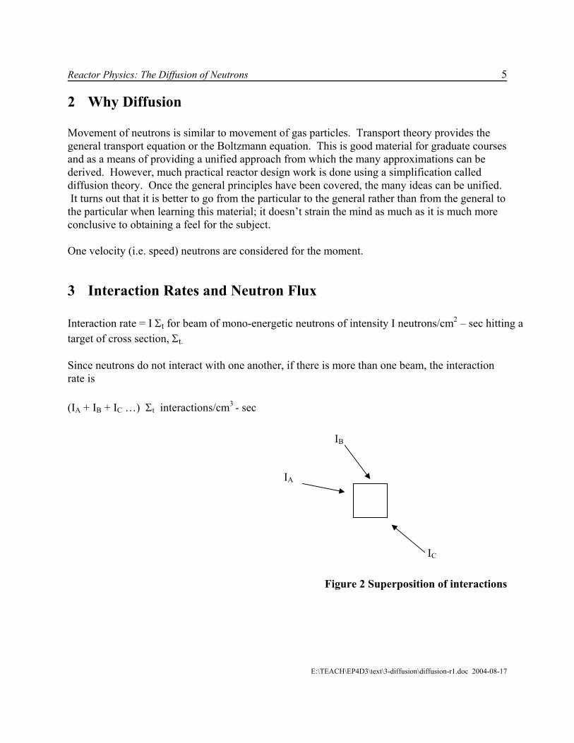
3 Interaction Rates and Neutron Flux Interaction rate = I Σt for beam of mono-energetic neutrons of intensity I neutrons/cm2 – sec hitting a target of cross section, Σt. Since neutrons do not interact with one another, if there is more than one beam, the interaction rate is (IA + IB + IC …) Σt interactions/cm3 - sec

IB IA IC

Figure 2 Superposition of interactions


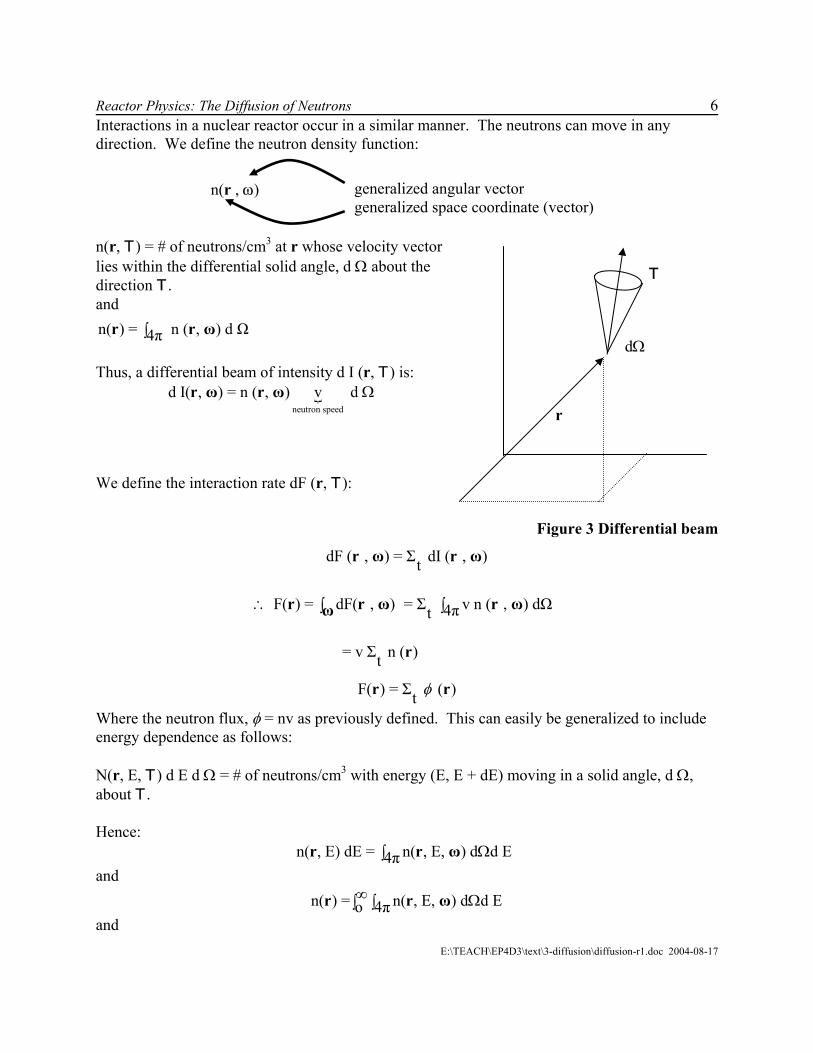
Reactor Physics: The Diffusion of Neutrons 6 Interactions in a nuclear reactor occur in a similar manner. The neutrons can move in any direction. We define the neutron density function:

n(r , ω) generalized angular vector

generalized space coordinate (vector) n(r, T) = # of neutrons/cm3 at r whose velocity vector lies within the differential solid angle, d Ω about the direction T. and

n( ) = n ( , ) d Ω4π∫r r ω Thus, a differential beam of intensity d I (r, T) is:

utron speed

v d ne

d I( , ) = n ( , ) Ωr ω r ω

r

T

dΩ

We define the interaction rate dF (r, T):

Figure 3 Differential beam

dF ( , ) = Σ dI ( , )tr ω r ω

F( ) = dF( , ) = Σ v n ( , ) dΩ 4πt∴ ∫ ∫r r ω r ωω

= v Σ n ( )t r

F( ) = Σ ( )t φr r

Where the neutron flux, φ = nv as previously defined. This can easily be generalized to include energy dependence as follows: N(r, E, T) d E d Ω = # of neutrons/cm3 with energy (E, E + dE) moving in a solid angle, d Ω, about T. Hence:

n( , E) dE = n( , E, ) d d E 4π Ω∫r r ω and

n( ) = n( , E, ) d d Eo 4π∞ Ω∫ ∫r r ω

and E:\TEACH\EP4D3\text\3-diffusion\diffusion-r1.doc 2004-08-17

Reactor Physics: The Diffusion of Neutrons 7 F( , E)dE = (E)n( , E)v(E)dEtΣr r

= number of interactions occurring per cm3 per sec at r in the energy interval dE.

= (E) ( , E)dEt φΣ r

Finally, F( ) = (E) ( , E)dE o t

∞Σ∫r rφ

Thus knowing the material properties, Σt, and the neutron flux, φ, as a function of space and energy, we can calculate the interaction rate throughout the reactor. We can similarly arrive at interaction rates for scattering, etc.

F (r) = (E) ( , E)dE , etc.oS S φ∞ Σ∫ r

Note: φ, neutron flux, is a scalar; whereas, most fluxes (ie. heat flux) are vectors. φ is not the flow of neutrons. There may be no flow of neutrons, yet many interactions may occur. The neutrons move in a random fashion and hence may not flow. φ is more closely related to densities. Just as mass and heat flow when there is a density difference in space, neutrons will exhibit a net flow when there are spatial differences in density. Hence we can have a flux of neutron flux!



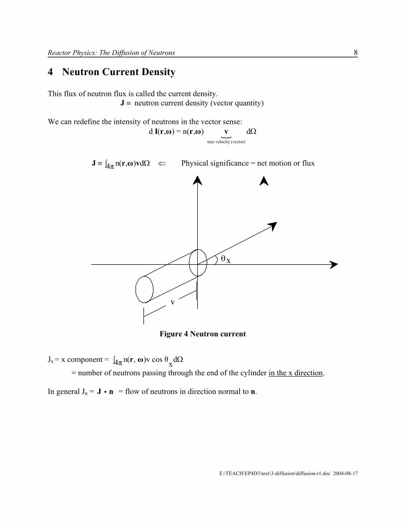
4 Neutron Current Density This flux of neutron flux is called the current density.

≡J neutron current density (vector quantity) We can redefine the intensity of neutrons in the vector sense:

true velocity (vector)

d ( , ) = n( , ) dΩI r ω r ω v

n( , ) d 4π≡ Ω∫J r ω v ⇐ Physical significance = net motion or flux

v

xθ

Figure 4 Neutron current

Jx = x component = n( , )v cos θ d4π x Ω∫ r ω

= number of neutrons passing through the end of the cylinder in the x direction. In general Jn = = flow of neutrons in direction normal to n. J ni



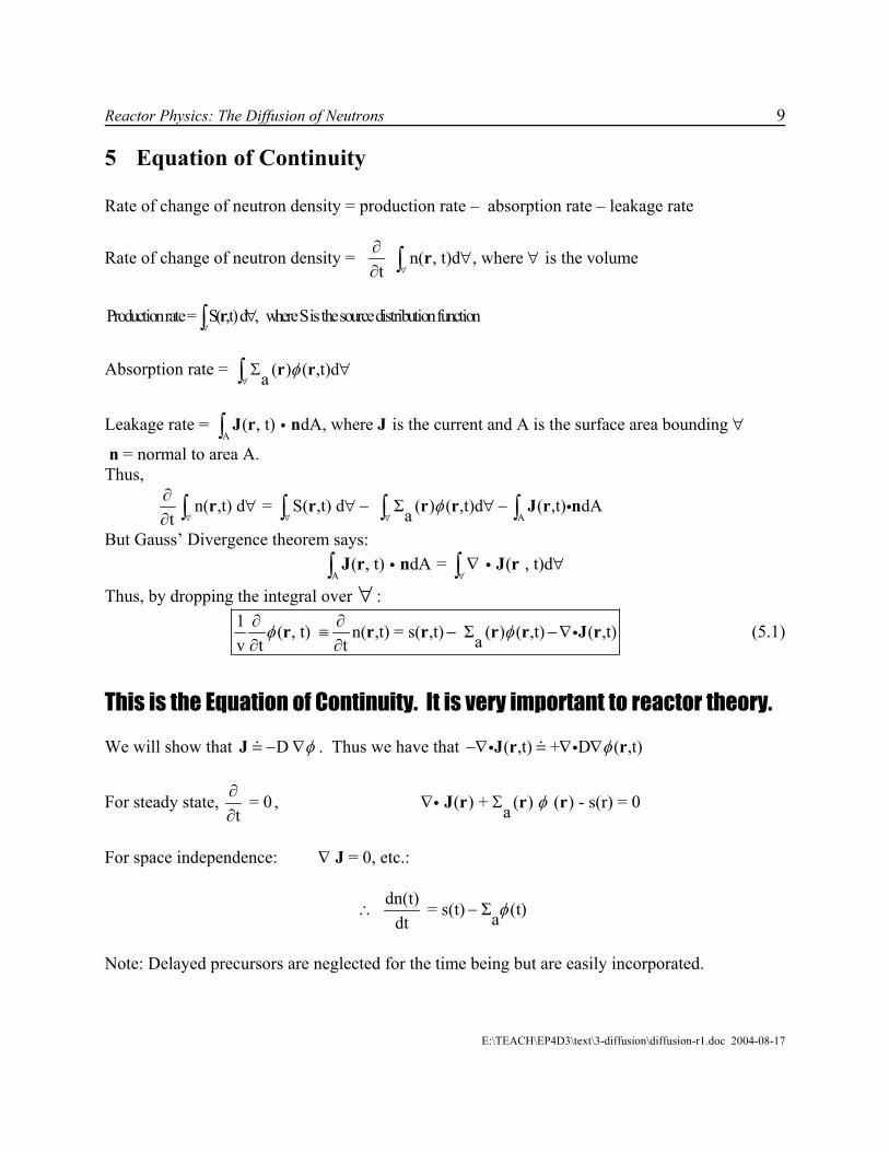
5 Equation of Continuity Rate of change of neutron density = production rate – absorption rate – leakage rate

Rate of change of neutron density = n( , t)d , where is the volumet ∀

∂∀ ∀

∂ ∫ r

Production rate = S( ,t) d , where S is the source distribution function

∀∀∫ r

Absorption rate = ( ) ( ,t)da∀

Σ ∀∫ r rφ

Leakage rate =

A( , t) dA, where is the current and A is the surface area bounding ∀∫ J r n Ji

n = normal to area A. Thus,

A

n( ,t) d = S( ,t) d Σ ( ) ( ,t)d ( ,t) dAat ∀ ∀ ∀

∂∀ ∀− ∀−

∂ ∫ ∫ ∫ ∫r r r r J r iφ n

But Gauss’ Divergence theorem says:

A( , t) dA = ( , t)d

∀∇ ∀∫ ∫J r n J ri i

Thus, by dropping the integral over ∀ : 1 ( , t) n( ,t) = s( ,t) Σ ( ) ( ,t) ( ,t)av t t∂ ∂

≡ − −∇∂ ∂

r r r r r Jiφ rφ (5.1)

This is the Equation of Continuity. It is very important to reactor theory. We will show that D − ∇J φ . Thus we have that ( ,t) + D ( ,t)−∇ ∇ ∇J r ri i φ

For steady state, = 0t∂∂

, ( ) + ( ) ( ) - s(r) = 0a φ∇ ΣJ r r ri

For space independence: ∇ J = 0, etc.:

dn(t) = s(t) Σ (t)adt

φ∴ −

Note: Delayed precursors are neglected for the time being but are easily incorporated.



6 Fick’s Law We apply Fick’s Law (from diffusion in liquids, gases, etc.) to the neutrons in order to supply a relationship between J and known quantities.

6.1 Derivation Fick’s Law was developed under the following assumptions:

1. The medium is infinite; 2. The medium is uniform, ie. ( );Σ ≠ Σ r 3. There are no neutron sources in the medium;

4. Scattering is isotropic in the laboratory coordinate system;

5. The neutron flux is a slowly varying position of position;

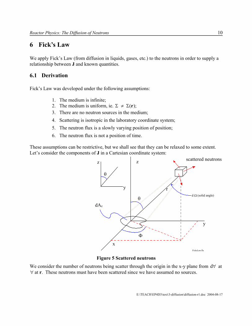
6. The neutron flux is not a position of time. These assumptions can be restrictive, but we shall see that they can be relaxed to some extent. Let’s consider the components of J in a Cartesian coordinate system:

z

y

x

z

y

scattered neutrons

FicksLaw.fla

r

dAz

θ

Φ

θ

d (solid angle)Ω

Figure 5 Scattered neutrons

We consider the number of neutrons being scatter through the origin in the x-y plane from d∀ at at r. These neutrons must have been scattered since we have assumed no sources. ∀


Reactor Physics: The Diffusion of Neutrons 11 The number of collisions/sec at r is: slowly varying

Σ ( ) ( )d = Σ ( )ds sφ φ∀ ∀r r r

assumed space independence Since the scattering is isotropic:

Zcos θ dA dΣ ( )s 24 r

∀rφπ

neutrons/sec

Head towards dAz from d∀ at r

But some are removed en route ( . (Note: As usual, we assume no buildup factor.) -Σ rte )

Thus cos dA-Σtr ( )(e ) ds 24 r

ZΣθ

φπ

∀r pass through the area dAz.

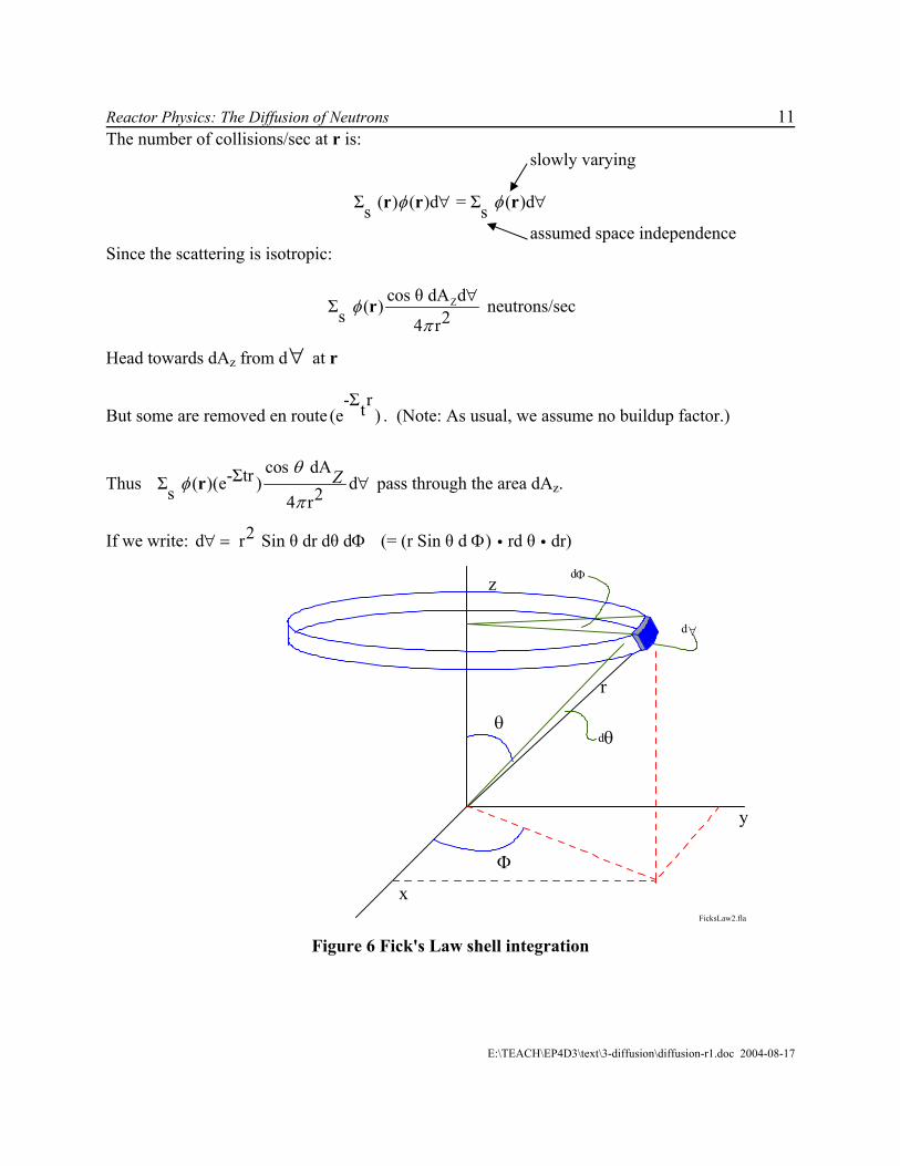
If we write: d r (= (r S2 Sin θ dr dθ d∀ = Φ in θ d ) rd θ dr)Φ i i

z

y

xFicksLaw2.fla

r

θ

Φ

θ

dΦ

d

∀d

Figure 6 Fick's Law shell integration


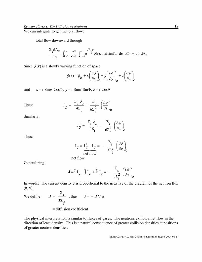
Reactor Physics: The Diffusion of Neutrons 12 We can integrate to get the total flow: total flow downward through

2 π/2Z

Z Z0 0 = 0

Σ dA -Σ r -s t e (r)cos sin dr d d J d4π

∞

Φ= =Φ =∫ ∫ ∫r

π

θφ θ θ θ A

Since φ (r) is a slowly varying function of space:

( ) = + x + y + zo x yo oo zφ φ φφ φ ∂ ∂ ∂

∂ ∂ ∂ r

and x = r Sin Cos , y = r Sin Sin , z = r Cosθ θ θΦ Φ

Thus: Σ Σs o sJ + Z 24Σ z6Σ ot t

∂ − = ∂

φ φ

Similarly: Σ Σs o sJ Z 24Σ z6Σ ot t

φ φ∂ + = − ∂

Thus: ΣaJ J J Z Z Z 2 z3Σ otnet flow

∂ + −= − = − ∂ φ

net flow Generalizing:

Σsi J + j J + k J x y z 2 z3Σ ot

∂ = = − ∂ J φ

In words: The current density J is proportional to the negative of the gradient of the neutron flux (n, v).

We define 2

ΣsD 3Σ

t

= , thus = D φ− ∇J

= diffusion coefficient The physical interpretation is similar to fluxes of gases. The neutrons exhibit a net flow in the direction of least density. This is a natural consequence of greater collision densities at positions of greater neutron densities.


Reactor Physics: The Diffusion of Neutrons 13 6.2 Validity of Fick’s Law We re-evaluate each assumption in turn: 1. Infinite medium. This assumption was necessary to allow integration over all space but

flux contributions are negligible beyond a few mean free paths due to the factor,

Thus as long as we are at least a few mean free paths from the reactor extremities, all is okay. Corrections can be made at the reactor surfaces as shown later in this chapter.

-Σ rte .

2. Uniform medium. A non-uniform medium ( requires a re-evaluation of the

derivation of Fick’s Law. Now the interaction rate, Σ

Σ = Σ ( ))s s r

S φ, is a function of space due to both φ and Σ variations in space. Detailed calculations show, however, that the extra current (ie. scattering) contributions caused by a locally larger ΣS are exactly cancelled by larger

attenuations ((e-Σ r -(Σ + Σ )rt s a= e ) iff (if and only if) or /s a s t∑ >> ∑ ∑ ∑ = constant.

It should be noted however that ΣS (r) can lead to large values of ( )∂∂

rrφ which violates

assumption (e).

3. Sources. As per assumption (a), we can get away with sources as long as they are more

than a few mean free paths away. 4. Isotropic scattering. Anisotropic scattering can be corrected for by detailed

considerations of transport theory in which D is re-evaluated:

Σ + Σ /DΣ 1 + 3DΣ µD t as s ln 2 Σ 1 + 3DΣ µ Σ Σ /Da st a

= −

Where µ cosθ≡ (average of the scattering angle in the lab system)

23A

=

Expanding the equation in D, above: 1D =

3Σ (1 µ)(1 4Σ /5Σ +...) t a− − t



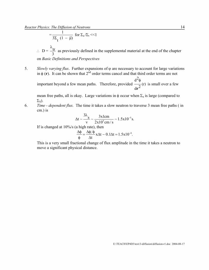
= 13Σ (1 µ)t −

for Σa /Σt <<1

λ tr D = 3

∴ as previously defined in the supplemental material at the end of the chapter

on Basic Definitions and Perspectives

5. Slowly varying flux. Further expansions of ϕ are necessary to account for large variations in φ (r). It can be shown that 2nd order terms cancel and that third order terms are not

important beyond a few mean paths. Therefore, provided 2d

(r)2d

φ

r is small over a few

mean free paths, all is okay. Large variations in φ occur when Σa is large (compared to ΣS).

6. Time - dependent flux. The time it takes a slow neutron to traverse 3 mean free paths ( in cm.) is

55

3 3x1cmst 1v 2x10 cm / s

−.5x10 s.λ

∆ ∼ ∼ ∼

If is changed at 10%/s (a high rate), then

6x t 0.1 t 1.5x10 .t

−∆φ ∆φ φ= ∆ ∆ =

φ ∆∼

This is a very small fractional change of flux amplitude in the time it takes a neutron to move a significant physical distance.



7 Question: What about the Conservation of Momentum and Energy?

Question: This neutron balance equation:

n( , t) s(r , t) Σ (F) ( , t)atφ∂

= −∂r r + D( ) ( , t)φ∇ r ri

Is similar to the conservation of mass in fluids: ρ S ρvt

∂= −∇

∂i

Why do we not also consider the conservation of momentum and energy? Solution: Conservation of momentum and energy is used on a neutron-nucleus interaction level. Recoils, etc. lead to cross sections, which are input into the neutron balance equation. Compare this to fluid mechanics. The neutrons don’t interact with each other but fluid particles do. Hence the fluid mass, energy, and momentum equations are tightly linked. The neutrons affect each other only via temperature changes, etc., brought about by fissioning, whereas, fluid particles shear off each other and with the walls. This is a fundamental difference. In short:

1. Because of treatment of Σ as effective area of interaction

2. Too complicated.

3. Neutrons do not interact with each other!



8 The Diffusion Equation We return now to the neutron balance equation:

n( ,t) = s( ,t) Σ ( ) ( ,t) ( ,t)at∂

− φ −∇∂

r r r r J ri (8.1)

and substitute = D ( ,t)− ∇φJ r

to give

n( ,t) = s( ,t) Σ ( ) ( ,t)+ D ( ,t)at∂

− φ ∇ ∇φ∂

r r r r ri

If D = constant w.r.t. r then (using n v = φ) 2

a1 ( , t) = S( ,t) Σ ( ) ( , t) + D ( ,t)v t

∂φ − φ ∇

∂r r r r φ r ←Neutron diffusion equation

For steady state 1 ( ,t) = 0v t

∂φ

∂r . This steady state diffusion equations is also known as the

“scalar Helmholtz equation”. If s (r) = 0 as well, it is sometimes called the “buckling equation” in analogy to the equation governing the buckling of beams in strength of materials. It is also known as the “wave equation” in analogy to vibrating strings, etc.



9 Boundary Conditions for the Steady State Diffusion Equation For this type of equation the following applies: On the boundaries of a region in which φ satisfies the differential equation, either φ, or the normal derivative of φ, or a linear combination of the two must be specified. Both φ and its normal derivative cannot be specified independently.

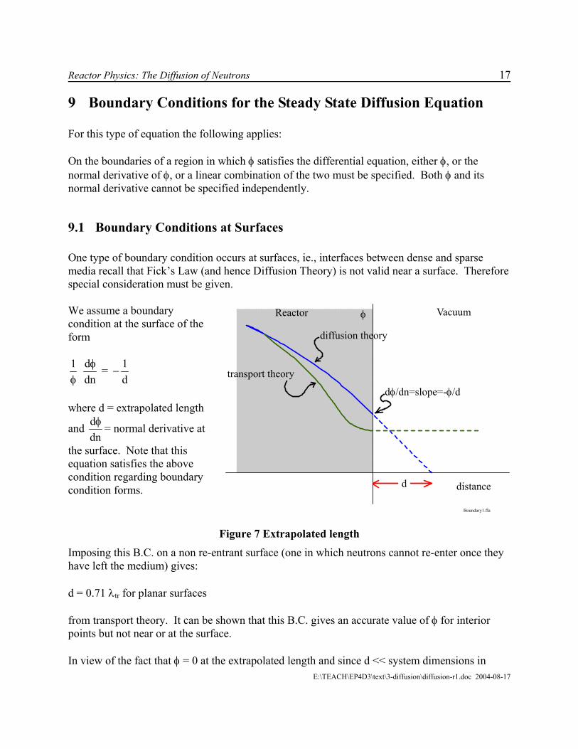
9.1 Boundary Conditions at Surfaces One type of boundary condition occurs at surfaces, ie., interfaces between dense and sparse media recall that Fick’s Law (and hence Diffusion Theory) is not valid near a surface. Therefore special consideration must be given. We assume a boundary condition at the surface of the form

Reactor Vacuum

distanced

φ

diffusion theory

transport theory

dφ/dn=slope=-φ/d

Boundary1.fla

1 d 1 =

dn dφ

−φ

where d = extrapolated length

and ddnφ = normal derivative at

the surface. Note that this equation satisfies the above condition regarding boundary condition forms.

Figure 7 Extrapolated length

Imposing this B.C. on a non re-entrant surface (one in which neutrons cannot re-enter once they have left the medium) gives: d = 0.71 λtr for planar surfaces from transport theory. It can be shown that this B.C. gives an accurate value of φ for interior points but not near or at the surface.

E:\TEACH\EP4D3\text\3-diffusion\diffusion-r1.doc 2004-08-17 In view of the fact that φ = 0 at the extrapolated length and since d << system dimensions in

Reactor Physics: The Diffusion of Neutrons 18 practical situations, the above B.C. is replaced with little error by: The solution to the diffusion equation vanishes at the extrapolation distance beyond the edge of a free surface. The assumptions inherent in the above should be carefully noted.

Since D = diffusion coefficient = λ tr3

and D ~ 1 cm,

d = .71 λ ~.71 3 ~ 2 cm << reactor size (meters)tr∴ ×

(surface) 0∴ φ ≈

9.2 Boundary Conditions at an Interface At an interface, there is no accumulation of neutrons. Therefore:

(JA)n = (JB)n where n=normal direction

ie. the neutron current in region A = that of B Also, n (r, t, …) and φ (r, t, …) are continuous across the interface.

9.3 Other Conditions Physical requirements:

1. A negative or imaginary flux has no meaning. Hence: the solution to the diffusion equation must be real, non-negative and single valued in those regions where the equation applies.

2. φ ≠ ∞ except for singular points of source distributions. These two constraints

serve to eliminate extraneous functions from the solution.



9.4 Summary of Boundary Conditions

1. φ = φ at an interface

2. J = J

3. φ defined at a surface

4. J = defined

5. φ finite

6. φ > 0 and real



10 Elementary Solutions of the Steady State Diffusion Equation We have previously shown the Steady State Diffusion Equation to be

20 S( ) Σ ( ) ( )+D ( )a= − φ ∇ φr r r r

Defining D2 2L = [cm ]; L diffusion lengthΣa

≡ ≡

12 = 2 DL

S∇ φ− φ − (10.1)

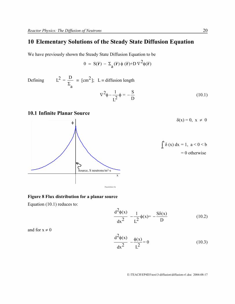
10.1 Infinite Planar Source δ(x) = 0, x 0≠

Source, S neutrons/m2-sx

φ

PlanarInfinite1.fla

b

aδ (x) dx = 1, a < 0 < b

= 0 otherwise∫

Figure 8 Flux distribution for a planar source

Equation (10.1) reduces to: 2d (x) 1 S (x)= 2 2 Ddx L

φ (x)δ− φ − (10.2)

and for x ≠ 0 2d (x) (x) = 02 2dx L

φ φ− (10.3)


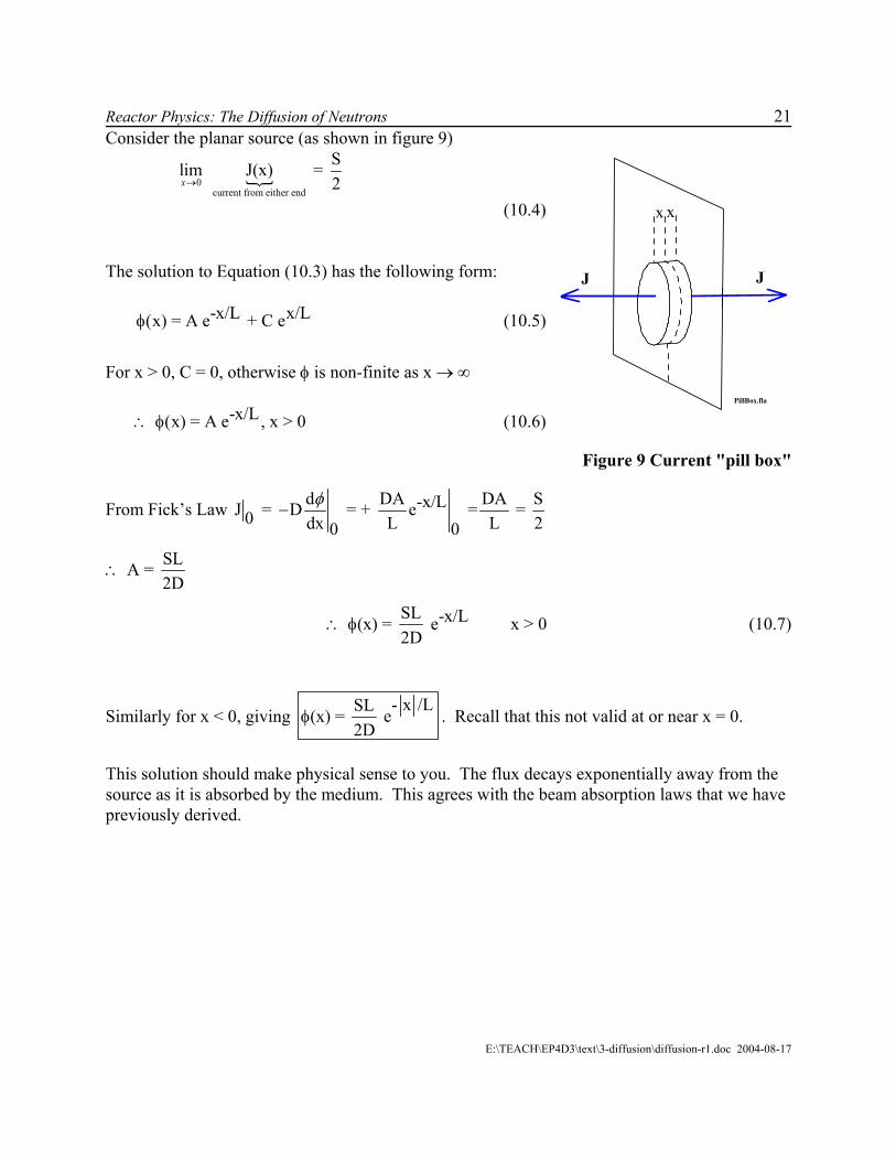
Reactor Physics: The Diffusion of Neutrons 21 Consider the planar source (as shown in figure 9)

0current from either end

lim J(x) =→x

-x/L x/L(x) = A e + C eφ

-x/L (x) = A e , x > 0

S 2

(10.4)

PillBox.fla

x x

JJ

The solution to Equation (10.3) has the following form:

(10.5)

For x > 0, C = 0, otherwise φ is non-finite as x → ∞

(10.6) ∴ φ

Figure 9 Current "pill box"

From Fick’s Law d DA DA-x/LJ = D = + e = = 0 dx L L 20 0

φ−

S

SL A = 2D

∴

SL -x/L (x) = e x > 02D

∴ φ (10.7)

Similarly for x < 0, giving - x /LSL(x) = e

2Dφ . Recall that this not valid at or near x = 0.

This solution should make physical sense to you. The flux decays exponentially away from the source as it is absorbed by the medium. This agrees with the beam absorption laws that we have previously derived.



10.2 Point Source in an Infinite Medium For a point source, it is appropriate to work in spherical coordinates:

surface area = 4πr2

r

Sδ(r)

Source1.fla

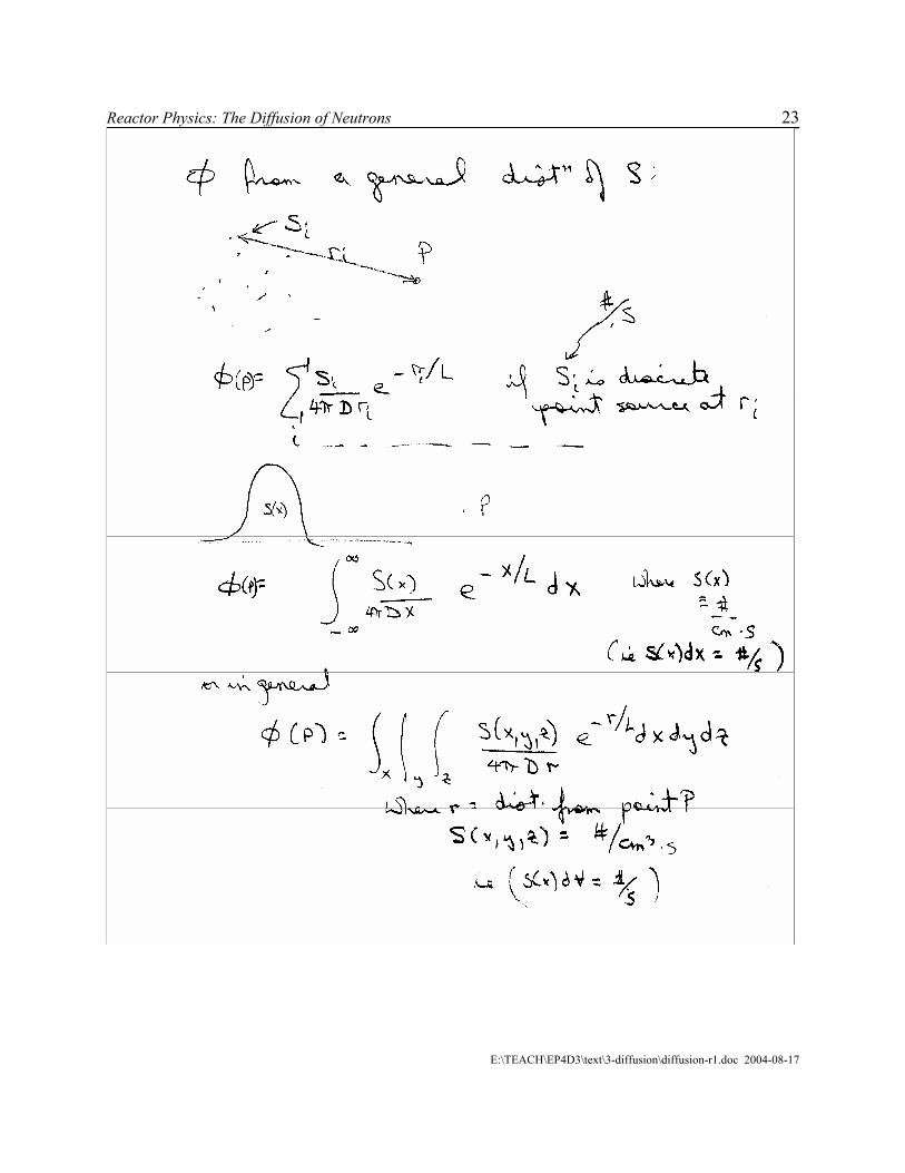
22 21 d d 1r

dr drr Lφ− φ = δS (r) (10.8)

where the source, S, is at r = 0.

Figure 10 Point source

Now 24 r J(r) S (r) Sπ = δ =

2r 0

Slim r J(r)4δ →

∴ =π

(10.9)

We define a change of variable

2

2 2ω 1ω=r - ω=0

r L∂

φ⇒∂

(10.10)

and, therefore, as before: -r/L r / L=Ae Ceω +or

-r/L r/Le e=A +C and C=0 as before.r r

φ

Now,

r / L2

d 1 1J=-D DA edx rL r

−φ = +

2 r / L 0 / Lr 0

r 0

r Sr J DA 1 e DAe DAL 4

− −=

=

∴ = + = = = π

r / LS SA= , = e4πD 4 Dr

−∴ ∴ φπ

Note: In the above two cases, as in most reactor cases, the flux, φ, is proportional to the source strength, S.



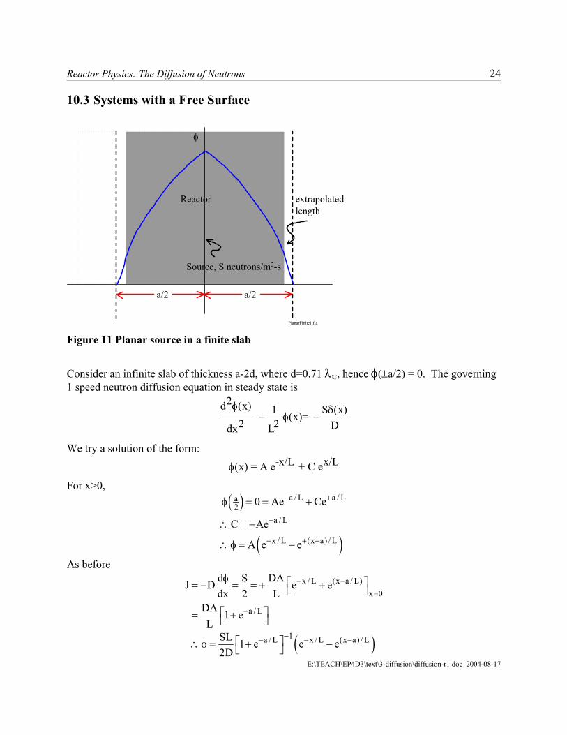
10.3 Systems with a Free Surface

Reactor

Source, S neutrons/m2-s

extrapolated length

a/2

φ

PlanarFinite1.fla

a/2

Figure 11 Planar source in a finite slab

Consider an infinite slab of thickness a-2d, where d=0.71 λtr, hence φ(±a/2) = 0. The governing 1 speed neutron diffusion equation in steady state is

2d (x) 1 S (x)= 2 2 Ddx L

φ (x)δ− φ −

We try a solution of the form: -x/L x/L(x) = A e + C eφ

For x>0,

( )

( )

a / L a / La2

a / L

x / L (x a) / L

0 Ae Ce

C Ae

A e e

− +

−

− + −

φ = = +

∴ = −

∴φ = −

As before

x / L (x a / L)x 0

a / L

d S DAJ D e edx 2 L

DA 1 eL

− −=

−

φ = − = = + +

= +


( )1a / L x / L (x a) / LSL 1 e e e2D

−− − − ∴φ = + −

Reactor Physics: The Diffusion of Neutrons 25 From symmetry, we conclude

( )( )

( )

1 x / L ( x a) / La / LSL 1 e e e2D

sinh a 2 x / 2LSL2D cosh a / 2L

− − −− ∴φ = + −

− =

We could have started with A cosh(x / L) Csinh(x / L)φ = +to get the same answer. Lamarsh suggests using hyperbolic trial solutions for finite media and exponentials for infinite media for the following reasons:

1. Sinh x has a zero – good for finite media 2. at x = ∞ - good for infinite media xe− → 03. sinh x and cosh x →∞ at x = ∞ - bad for infinite media 4. cosh x is an even function – good for symmetry.

When working with distributed sources, solutions usually are:

1. Cosine, sine for Cartesian coordinates 2. Bessel for cylindrical geometry.

Math aside:

x / L (x a )L a / 2L x / L (x a ) / L

a / L a / 2L a / 2L

(a 2x) / 2L (a 2x) / 2L

e e e (e e )1 e e ee e sinh[(a 2x) / 2L)]

2cosh(a / 2L) cosh(a / 2L)

− − − −

− −

− −

− −=

+ −− − −

= =

x x x xe e e esinh x , cosh x

2 2

− −− += =



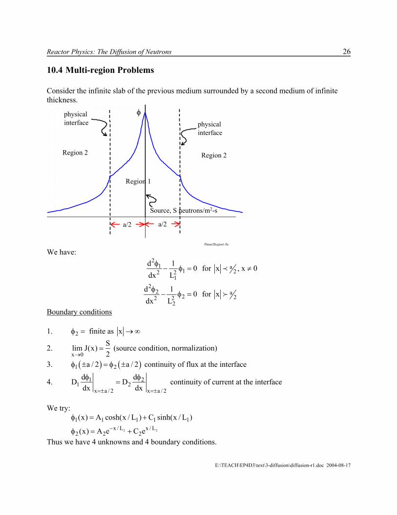
10.4 Multi-region Problems Consider the infinite slab of the previous medium surrounded by a second medium of infinite thickness.

Region 1

Source, S neutrons/m2-s

Region 2 Region 2

physicalinterface

physicalinterface

a/2

φ

Planar2Region1.fla

a/2

We have:

21 a

1 22 21

22 a

2 22 22

d 1 0 for x , x 0dx L

d 1 0 for xdx L

φ− φ = ≠

φ− φ =

≺

Boundary conditions 1. 2 finite as xφ = →∞

2. x 0

Slim J(x) (source condition, normalization)2→

=

3. ( ) ( )1 2a / 2 a / 2 continuity of flux at the interfaceφ ± = φ ±

4. 1 21 2

x a / 2 x a / 2

d dD D continuity of current at the interfacedx dx=± =±

φ φ=

We try:

2 2

1 1 1 1x / L x / L

2 2 2

(x) A cosh(x / L ) C sinh(x / L )

(x) A e C e−

φ = +

φ = +

1

Thus we have 4 unknowns and 4 boundary conditions.


Reactor Physics: The Diffusion of Neutrons 27 Immediately: C2=0 from B.C. (1) above. From (2):

1 1 1 1x / L x / L x / L x / L

1 1 1 1 11

1 10 x 0 x 0

S d D A e e D C e eJ(0) D2 dx L 2 L 2

− −

= =

φ − += = − = − −

1

11

SLC2D

∴ = −

From B.C. (3)

2a / 2L11 2

1 1 1

a SL aA cosh sinh A e2L 2D 2L

−− + =

From B.C. (4)

2a / 2L1 1 2 2

1 1 1 2

D A a S a D Asinh cosh eL 2L 2 2L L

−− + =

2 equations in 2 unknowns Solve for A1 and A2

Solving gives:

1 1 2 1 2 1 11

1 2 1 1 1 2 1

SL D L cosh(a / 2L ) D L sinh(a / 2L )A2D D L cosh(a / 2L ) D L sinh(a / 2L )

+=

+

1a / 2L

1 22

2 1 1 1 2 1

SL L eA2 D L cosh(a / 2L ) D L sinh(a / 2L )

=+

Therefore, we know φ1 and φ2 . Notes:

1. φ1 and φ2 are proportional to S. 2. It can be shown that φ is continuous at ±a/2 and that dφ/dx is not

continuous but D dφ/dx is. This results from the boundary conditions imposed. Only if D1=D2 is continuous.



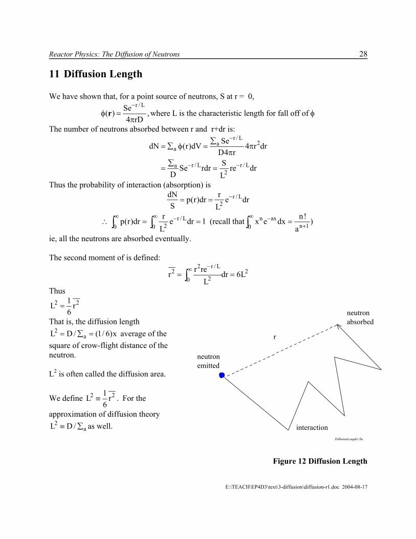
11 Diffusion Length We have shown that, for a point source of neutrons, S at r = 0,

r / LSe( ) , where L is the characteristic length for fall off of

4 rD

−φ =

πr φ

The number of neutrons absorbed between r and r+dr is:

r / L2a

a

r / L r / La2

SedN (r)dV 4 r drD4 rSSe rdr re dr

D L

−

− −

∑= ∑ φ = π

π∑

= =

Thus the probability of interaction (absorption) is

r / L2

dN rp(r)dr e drS L

−= =

r / L n ax2 n0 0 0r np(r)dr e dr 1 (recall that x e dx )

L a∞ ∞ ∞− −

+1!

∴ = = =∫ ∫ ∫

ie, all the neutrons are absorbed eventually. The second moment of is defined:

2 r / L

2 220

r rer dL

−∞= =∫ r 6L

Thus 2 21L r

6=

neutronemitted

interaction

neutron absorbed

r

DiffusionLength1.fla

That is, the diffusion length average of the

square of crow-flight distance of the neutron.

2aL D / (1/ 6)= ∑ = x

L2 is often called the diffusion area.

We define 2 1L6

≡

a∑

2r . For the

approximation of diffusion theory as well. 2L D /≡

Figure 12 Diffusion Length




About this document: back to page 1

Author and affiliation: Wm. J. Garland, Professor, Department of Engineering Physics, McMaster University, Hamilton, Ontario, Canada Revision history: Revision 1.0, 2001.07.10, initial creation from hand written notes. Revision 1.1 2004.08.17, typo correction. Source document archive location: D:\TEACH\EP4D3\text\3-diffusion\diffusion-r1.doc Contact person: Wm. J. Garland Notes:

reactor physics: the diffusion of neutrons - …nuceng.ca/ep4d3/text/3-diffusion-r1.pdfreactor...

Documents