University of Rhode Island University of Rhode Island

DigitalCommons@URI DigitalCommons@URI

Open Access Dissertations

2018

Diffusion of Ultra-Cold Neutrons in Randomly Rough Channels Diffusion of Ultra-Cold Neutrons in Randomly Rough Channels

Sarah Elizabeth Brent University of Rhode Island, sbrent@uri.edu

Follow this and additional works at: https://digitalcommons.uri.edu/oa_diss

Recommended Citation Recommended Citation Brent, Sarah Elizabeth, "Diffusion of Ultra-Cold Neutrons in Randomly Rough Channels" (2018). Open Access Dissertations. Paper 720. https://digitalcommons.uri.edu/oa_diss/720

This Dissertation is brought to you for free and open access by DigitalCommons@URI. It has been accepted for inclusion in Open Access Dissertations by an authorized administrator of DigitalCommons@URI. For more information, please contact digitalcommons@etal.uri.edu.

DIFFUSION OF ULTRA-COLD NEUTRONS IN RANDOMLY ROUGH

CHANNELS

BY

SARAH ELIZABETH BRENT

A DISSERTATION SUBMITTED IN PARTIAL FULFILLMENT OF THE

REQUIREMENTS FOR THE DEGREE OF

DOCTOR OF PHILOSOPHY

IN

PHYSICS

UNIVERSITY OF RHODE ISLAND

2018

DOCTOR OF PHILOSOPHY DISSERTATION

OF

SARAH ELIZABETH BRENT

APPROVED:

Dissertation Committee:

Major Professor Alexander Meyerovich

Leonard Kahn

David Freeman

Nasser H. Zawia

DEAN OF THE GRADUATE SCHOOL

UNIVERSITY OF RHODE ISLAND

2018

ABSTRACT

This thesis deals with ultra cold neutrons, or, more precisely, with beams

of ultra-cold neutrons. ultra-cold neutrons are longwave particles produced in a

reactor from which they are coming to experimental cells through narrow channels.

The beams are collimated so that the distribution of longitudinal and transverse

velocities is narrow. The energies of the neutrons that we consider as ultra cold

are somewhere around 100neV .

Neutrons with such low energies have long wavelengths; λ ∼ 100nm. Neutral

particles with such large wavelengths exhibit nearly (locally) specular reflection

when reflected by the solid surfaces at almost any angle of incidence.

The number of ultra-cold neutrons available for experiment is extremely small.

Therefore, a major experimental challenge is not to lose any particles while they

travel from the reactor to the lab. Some of the main losses occur in the chan-

nel junctions when the neutrons disappear into the gaps between the overlapping

channels. We explore the possibility of recovering some of these otherwise ”lost”

neutrons by making the inside surfaces of the junctions rough: scattering by the

surface roughness can send some of the neutrons back out of the gap. This prac-

tical goal made us to re-examine diffusion of neutrons through rough channels

which is by itself an interesting problem. We assume that the correlation func-

tion of random surface roughness is either Gaussian or exponential and investigate

the dependence of the mean free path on the correlation radius R of the surface

inhomogeneities. My results show that in order to ensure better recovery of the

”lost” neutrons the walls of the junction should be made rough with the exponen-

tial correlation function of surface roughness with as small a correlation radius as

possible. The results also show that the diffusion coefficient and the mean free

path of UCN in rough channels exhibit a noticeable minimum at very small values

of the correlation radius. This minimum sometimes has a complicated structure.

The second goal is the study of UCN in Earth’s gravitational field. One of the

most interesting features of ultra-cold neutrons is a possible quantization of their

vertical motion by the Earth’s gravitational field: the kinetic energies are so low

that they become comparable to the energy of neutrons in Earth’s gravitational

field. This results in quantization of neutron motion in the vertical direction. The

energy discretization occurs on the scale of several peV.

In the first part of my thesis I ignore the presence of the gravitational field

and look at the transport of neutrons through rough waveguides in the absence of

gravity. The effects of gravity are be explored in the last part. To streamline the

transition I use the common notations suitable for both types of problems.

More specifically, I am studying the diffusion of ultra-cold neutrons in the

context of the experiments done at ILL in Grenoble in the frame of the multi-

national GRANIT collaboration. The parameters used in numerical calculations

are the ones most common to ILL experiments. I will be calculating the diffusion

coefficient and the mean-free path (MFP) under the conditions of the quantum

size effect. Specifically I look at the dependence of the diffusion coefficient and the

MFP on the correlation radius of surface inhomogeneities. R. In the second and

third parts of the thesis I include the study of the neutron diffusion accompanied

by slow continuous disappearing of neutrons as a result of penetration into the

channel walls. This includes calculating the number of neutrons N(t = τex, h, R),

where τex is the experimental value of the time of flight in GRANIT experiments

and h is the channel width. I look not only at the square well geometry, but will

also include the effects of the Earth gravitational field. The results show that while

the neutrons in the square well potential disappear almost immediately, the small

perturbation near the bottom of the well caused by the presence of the Earth’s

gravitational field drastically changes the results and is solely responsible for the

observed exit neutron count in GRANIT experiments. The shape of the curves

describing the exit neutron count on the width of the waveguide is extrememly

robust. Out brute force calculations also confirms that the earlier biased diffusion

approximation is quite accurate.

ACKNOWLEDGMENTS

I would like to acknowledge first and foremost my thesis adviser, Professor

Alexander Meyerovich. I am deeply grateful for the guidance, advice, tremendous

insight and immeasurable patience and support that you provided to me over the

past 6 years.

I would also like to acknowledge Professor Leonard Kahn for the wonderful

teacher that he is, for the encouragement that he provided even at times when I

had doubts, and for the many informal conversations we had on a vast array of

topics.

Sincere thanks go out to Professor Gerhard Muller, for all the physics tools

he gave me over the past 6 years, as well as the many enjoyable and insightful

conversations.

Thanks to Professor Peter Nightingale, for the crazy difficult classes that

provided me with great challenges, as well as for his wit and generosity in sharing

knowledge about music, history and other topics outside of physics.

Thank you to Professor Richard McCorkle for being a great support to me in

my function as a TA, as well as always having a pleasant outlook on life.

Thank you to Linda Connell for always cleaning up my administrative messes,

as well as being a great friend and support over the last 6 years.

Thank you to Steve Pellegrino for helping me with countless technology and

computer problems, as well as for his friendship.

Thank you to David Notorianni for always fixing anything that went wrong

in the labs or offices, as well as for having a kind heart behind the rough exterior.

Thank you to Professor Donna Meyer, for introducing me to engineering which

has become another passion of mine, as well as for being a great role model for a

woman in the hard sciences. I have great admiration for you.

v

Thank you to Professor Stephen Barber, who though not a disciple of the

sciences, I have learned so much from, not only in English literature, theory and

history but from who you are as a person. You are one of the most generous and

loving people I know, thank you for sharing yourself with me, I’m a better person

because of it.

Thank you to my dear friend Mauricio Escobar, who has always been a stellar

friend as well as a confident and support, even after he himself was done with his

Ph.D.

Thank you to Eden Uzrad and the entire Uzrad family in Israel, whom I got to

know very well over the course of my Ph.D. Thank you for all the support you gave

me, for your generosity, and for opening my eyes about your beautiful country.

Thank you to the woman of my life, Cecile Cres, whom I’ve been lucky to have

known since high school. You always encouraged me to pursue my passions, and

I thank you so much for being my greatest confident, as well as source of comfort

and support in my life.

Lastly, but certainly not least, a huge thank you to my parents for the educa-

tion they gave me, for always allowing me to follow my dreams, and providing me

with endless support in all my endeavors. In particular I would like to thank my

mom, who has always had my back 100 percent of the time, even at times when

she didn’t agree with my decisions. I wouldn’t be the person I am today without

you

vi

DEDICATION

This thesis is dedicated to the two most important women in my life who

have loved and encouraged me always. To my incredibly strong and bright mother,

Antoinette Duymovitsh, whom I admire so much, and to whom I owe everything.

And to my partner Cecile who encourages and supports me unconditionally on this

wild and fun ride called life, and from whom I learn daily.

vii

Contents

ABSTRACT ii

Acknowledgements vi

List of Tables xii

List of Figures xiii

Chapter 1. Introduction 1

1.1. Preliminary Comments 1

1.2. GRANIT Experiment 8

1.3. Notations and Dimensionless Variables 14

1.4. Theoretical Background 17

Chapter 2. Di¤usion Coe¢ cient and Mean Free Path in a Rough Waveguide 26

2.1. Introductory Comments 26

2.2. The Di¤usion Coe¢ cient 27

2.3. Mean Free Path 28

2.4. Numerical Results 29

2.5. Conclusions 37

viii

Chapter 3. Neutron Beams between Absorbing Rough Walls: Square Well

Approximation 44

3.1. Description of Problem 44

3.2. Wavefunction for the Square Well 48

3.3. Transition Probabilities and Neutron Count 50

3.4. Numerical Results 52

3.5. Conclusions 60

Chapter 4. Neutrons in the Rough Waveguide in the Presence of Gravity 67

4.1. Gravity-Imposed Changes: Similarities and Di¤erences with the

Previous Chapter 67

4.2. Results from the Preceding Work: the Biased Di¤usion Approximation 70

4.3. Exact Calculation of the Absorption Time 75

4.4. Numerical Results 78

4.5. Conclusions 85

Chapter 5. Summary and Conclusions 96

5.1. Main Conclusions 96

5.2. Recommendations for Future Work 99

Appendix A. Dimensionless Transition Probabilities 101

Appendix B. Asymptotic Expansion for Transition Probabilities for Surfaces

with Exponential Roughness Correlator 103

ix

Appendix C. Diagonal Elements of Transition Probabilities for the Biased

Di¤usion Approximation 105

Bibliography 107

x

List of Figures

1.1 Sketch of the experimental cell with a neutron beam between

two plates. The neutrons bounce between the "rough" ceiling

and "smooth" �oor. The neutrons with low vertical velocity,

which do not reach the ceiling get to the detector. 9

1.2 The GRANIT experiment: a more technical sketch of the

experiment as a whole. The experimental cell is on the right. 11

1.3 "Rough" ceiling mirror. The patches 1-5 represent the spots

where the roughness has been measured using vertical scanning

interferometry. 13

2.1 Minima of the di¤usion coe¢ cient d(r) as a function of the

correlation radius for the Gaussian inhomogeneities. The

di¤usion coe¢ cient starts growing again at larger r. 32

2.2 Di¤usion coe¢ cient d (r) for the Gaussian surface correlator

over large range of r. The minima in d (r) cannot be resolved

on this scale. 33

xi

2.3 The next �gure (Fig.[2:4]) shows the di¤usion coe¢ cient for

the exponential correlation function of surface roughness. 34

2.4 Di¤usion for the surface inhomogeneities with the exponential

correlation function over large range of r. 35

2.5 Mean free path l (r) for the surface with Gaussian roughness

over wider range of r. 36

2.6 Mean free path for the surface with exponential roughness over

wider range of r. 37

2.7 Mean-free path l (r) for both Gaussian and exponential

correlation functions for small r. 38

2.8 MFP for Gaussian correlation function for various channel

widths h = 16, 8, 4. 39

2.9 MFP for Gaussian (1) and exponential (2) surface correlation

functions over a wide range of r. 40

2.10 Power law �tting for the MFP l (r) surfaces with the Gaussian

correlation function for r from 20 to 40. 41

2.11 The power law �t for MFP l (r) for Gaussian inhomogeneities

over the range of r from 40 to 60 42

2.12 Power law �t for d (r) the exponential surface correlation

function over a large range of r. 43

xii

3.1 Sketch of neutron beam entering the experimental cell: the

neutrons pass between rough "ceiling" and smooth "�oor". 45

3.2 Square well levels. 47

3.3 Coe¢ cients bj(h) Ref[3.3] as a function of the width of the

channel h for the square well. 50

3.4 Ne as a function of the cuto¤ parameter S1 for h = 8 and

r = 0:65. Here we can see the initial increase. 54

3.5 Neutron count as a function of the size of the matrix S1 for

h = 8 and r = 0:65. We can see how it saturates nicely, at

about S1 = 300. In this plot we are looking at Ne over a larger

scale. 55

3.6 Ne as a function of the size of the matrix S1 for h = 5 and

r = 0:65. We are looking at Ne closer scale, so that we can see

the inital increase and gradual saturation. 55

3.7 Saturation of the neutron count as a function of the size of the

matrix S1, for h = 5 and r = 0:65. 56

3.8 Ne as a function of the matrix size S1 for h = 3 and r = 0:65.

We are looking at Ne closer scale, so that we can see the inital

increase and gradual saturation. 56

3.9 Neutron count as a function of the cuto¤ parameter S1 and

r = 0:65 for h = 3. 57

xiii

3.10 Ne (h) as a function of h for r = 0:1. 58

3.11 Ne (h) as a function of h for r = 1. 59

3.12 Ne (h) as a function of h for r = 5. 60

3.13 Ne (h) as a function of h for r = 10. 61

3.14 Ne (h) as a function of h for r = 30. 62

3.15 Total neutron count Ne as a function of di¤erent correlation

radii r for small well width h = 3. 63

3.16 Total neutron count Ne as a function of di¤erent correlation

radii r for well width h = 5. 64

3.17 Total neutron count Ne as a function of di¤erent correlation

radii r for well width h = 7. 65

3.18 Total neutron count Ne as a function of di¤erent correlation

radii r for well width h = 9. 66

4.1 Sketch of the gravitational well as a function of z. 68

4.2 The �rst three eigenvalues for both the square well and the

gravitational well as a function of the well width h. For better

comparison, the bottom of the square well is chosen in the

middle of the bottom of the gravitational well, mgh=2, and is

drifting with h. The eigenvalues for the gravitational well are

the lower curves, for the SW-the upper. 69

xiv

4.3 A few coe¢ cients bj�s as a function of well width size h for

both the square (lower curves) and the gravitational wells

(upper curves). 70

4.4 The �rst nine coe¢ cients bj as a function of the width of the

channel h for the gravitational well. The lowest curve is b1 and

the highest b9. 71

4.5 The transition probabilities W1j0 as a function of j0exhibit the

peak around j0 = 100. 78

4.6 Potential with Earth�s gravity �eld. 80

4.7 Neutron exit count as a function of h, for experimental

parameters. 82

4.8 Neutron count as a function of h for correlation radius radius

of roughness r = 0:1. 83

4.9 Neutron count as a function of h for correlation radius of

roughness r = 1. This is approximately twice the experimental

value of r. 84

4.10 Neutron count as a function of h for correlation radius of

roughness r = 5. 85

4.11 Neutron count as a function of h for correlation radius of

roughness r = 10. 86

xv

4.12 Neutron count as a function of h for correlation radius of

roughness r = 20. 87

4.13 Neutron count as a function of h for correlation radius of

roughness r = 30. 88

4.14 Neutron count as a function of h for correlation radius of

roughness r = 50. 89

4.15 Neutron count as a function of h for correlation radius of

roughness r = 100. 90

4.16 Neutron count as a function of h for correlation radius of

roughness r = 500. 91

4.17 Neutron count as a function of h for correlation radius of

roughness r = 1000. 92

4.18 Neutron exit count for �xed well width at h = 9, over a large

range of r. 93

4.19 Neutron exit count for �xed well width at h = 5, over a large

range of r. 94

4.20 Neutron exit count for �xed well width at h = 3, over a large

range of r. 95

xvi

CHAPTER 1

Introduction

1.1. Preliminary Comments

The main goal of this thesis is to provide a rigorous theoretical description for

the di¤usion of ultra cold neutrons (UCN) through narrow rough channels, which

is based on the theory of quantum transport in systems with rough boundaries

formulated by Meyerovich et al.[1]-[12]. We look at two separate problems: dif-

fusion of the neutrons through rough waveguides on the way from the reactor to

the experimental cell and the neutron count for neutrons exiting experimental cell

with absorbing walls.

We use numerical computations to investigate the e¤ect of two types of random

roughness on the di¤usion coe¢ cient and use numerical methods to evaluate the

neutron count using the experimental values of input parameters. We analyze two

types of potentials inside the cell: one the idealized square well potential (SW)

and the other the SW potential with an addition of the gravitational �eld. The

experimental parameters were provided for us by our experimental collaborators

at the Institute Laue-Langevin (ILL) in Grenoble, France in the frame of the

GRANIT project.

1

2

The purpose of this multinational collaborative experimental and theoretical

work is two-fold: to investigate the quantization of the motion of UCN by the

Earth gravitational �eld and to create UCN with well-de�ned energies in the peV

range necessary for studies of fundamental forces in quantum �eld theory.

Typical UCN coming out of the reactor have large wavelengths, � s 100 nm.

Neutral particles with such large wavelengths exhibit nearly (locally) specular re-

�ection when re�ected by the solid surfaces at almost any angle of incidence. One

of the most interesting features of ultra-cold neutrons is their quantization in the

Earth gravitational �eld: the particle kinetic energies can be so low (� 1 peV)

that they become comparable to the gravitational energy of neutrons in Earth�s

gravitational �eld. This results in quantization of neutron motion in the vertical

direction. This discretization is illustrated in the sketch below showing the discrete

energy levels of neutrons in the Earth gravitational �eld. The energy discretization

occurs on the scale of several peV. The �rst experimental observation of such a

quantization was done by Nesvizhevsky et al. Ref.[14]-[24] by using the GRANIT

spectrometer (see below).

Ultra-cold neutrons are longwave particles produced in a reactor from which

they are coming to experimental cells through narrow channels containing various

mirrors and collimators. The UCN beams are collimated so that the distribution

of longitudinal and transverse velocities is narrow. The energies of the neutrons

that we consider as ultra-cold are somewhere around 100 neV, and below.

3

The particles in the beam that reach the cell have a relatively large horizontal

velocity and much smaller vertical velocities. Still standard collimation and cooling

methods are insu¢ cient to limit the vertical energies to the peV scale comparable

to gravitational energies. The typical UCN beam brought to the experimental cell

contains neutrons in thousands of occupied gravitational states making it virtually

impossible to study the quantization of vertical motion.

The purpose of the GRANIT spectrometer is to eliminate the particles in higher

gravitational states and leave only the ones in the few lowest states. This allows

one to achieve both goals: to study the quantization of neutron motion in the

gravitational �eld and to produce neutrons with well-de�ned energies in the peV

range.

The lower surface of the spectrometer is as close as possible to being perfectly

smooth, in order to make it to be a perfect re�ector which specularly re�ects the

UCN. The upper surface of the GRANIT cell has microscale roughness. This

"rough" ceiling scatters the UCN in higher gravitational states, which can reach

it. The scattered neutrons from the higher gravitational states eventually acquire

large vertical velocities su¢ cient to trigger penetration through the walls and dis-

appearance from the system. Due to this setup, only the UCN in low gravitational

states, which do not reach the rough ceiling, can continue bouncing along the �at

�oor and arrive at the exit neutron detector.

The use of rough mirrors as quantum state selectors is possible because the

very large horizontal velocities in the beam and peculiarities of quantization of the

4

vertical motion in the gravitational �eld. This kind of state selector is used or

is planned to be used, in numerous other applications not exclusive to GRANIT

experiments or to UCN beams. Some examples of these potential applications

include: the observation of quantum gravitational states for other ultra-cold par-

ticles and anti-particles in the context of the GBAR project at CERN [[28]-[32]];

the resolution of centrifugal quantum states in UCN in the "whispering gallery"

[[26],[27]]; the search for fundamental forces at extra-short range as predicted by

the grand uni�cation theory [[33]-[41]]; the test of the weak equivalence principle

[[39]-[42]]; the continual extension of understanding of quantum mechanics. Addi-

tionally, these GRANIT-like experiments could potentially be used to measure the

electric dipole moment of a neutron [[46],[47]], if it exists, help to search for the

potential neutron charge [[48],[49]], and make a precise measurement of neutron

lifetime [[50]].

The resolution and the quality of the observed quantum gravitational states of

UCN rely on the quality of the roughness of the upper surface of the GRANIT

cell. Meyerovich et al.. developed a theoretical framework in which they analyzed

the particle di¤usion along the random rough walls and linked it to the roughness

parameters of the rough mirror. The theory generally agrees with the experimental

results despite uncertainty in certain parameters.

Additionally, Meyerovich et al. [[52]-[55]] discovered that the shape of the

correlation function of surface inhomogeneities (CF) plays a very important role

in the di¤usion of UCN along rough walls. It turns out that the roughness-driven

5

transition probabilities between the states are directly proportional to the Fourier

image (the so-called power spectrum) of the CF. In previous work, Escobar et al.

[[8]] showed that within the biased di¤usion approximation all the information

about the surface imperfections can be accounted for in the neutron count as

a single parameter �, which is a complicated integral of the power spectrum.

However, in practice, it is impossible to create imperfections with a predetermined

CF on real surfaces, and even if it were possible it would be highly non-trivial to

identify this CF.

In order to increase the resolution of the observed quantum gravitational states

of the UCN in the GRANIT spectrometer, proper identi�cation of the surface

correlator is paramount. If one can establish a superior way to control the necessary

random roughness of the scatterer and absorber mirror, it will contribute greatly

to the optimization of results from the GRANIT experiment.

In the context of the theoretical background and numerical experiments, we

designate the shape of the CF explicitly, and analyze its potential impact on phys-

ical variables. In previous papers, Meyerovich et al. [[9]] have analyzed the gener-

ated rough surface by measuring it with the computational analog of STM needle

(scanning tunneling microscope). Unlike the CF used to generate the surface,

the correlator was extracted by direct computation and analyzed using various

�tting functions. Alternatively, the extracted correlator was fed directly into the

equations for the observables without the �tting functions. The reason for the im-

portance of the numerical experiments with the simulated surfaces lies in showing

6

how to avoid certain limitations that might stymie the dependable identi�cation

of a surface correlator for a real surface.

There is also a supplementary practical issue. The number of ultra-cold neu-

trons available for experiment is extremely small. Therefore, a major experimental

challenge is not to lose many particles while they travel from the reactor to the

lab. The main losses occur in the channel junctions when the neutrons get into

the gaps between the overlapping channels. Therefore the minimization of losses

in channel junctions becomes an important goal which will also be approached in

this thesis.

This thesis is arranged as follows:

In the remainder of Chapter 1, we will provide a fairly detailed description of

the experiment and its setup used by GRANIT to observe the quantum gravita-

tional states of the ultra cold neutrons. In particular we will describe the GRANIT

cell, and introduce the important parameters that are used to describe the rough-

ness of the surfaces of the GRANIT mirror. In section 2 we will discuss the details

of the mirror used in the newer experiments including the design and providing a

description of how they made the roughness. In section 3 we introduce the main

parameters and dimensionless variables. And, �nally, in section 4, we will pro-

vide the main equations and the theoretical framework for the quantum transport

equation and di¤usion.

In Chapter 2, we will explore the possibility of recovering these "lost" neutrons

that we discussed above by making the inside surfaces of the junctions rough:

7

scattering by the surface roughness can turn some of the neutrons back. This

practical goal made us to re-examine di¤usion of neutrons through rough channels

which is by itself an interesting general problem. We assume that the correlation

function of surface roughness is either Gaussian or exponential (see below) and

investigate the dependence of the mean free path on the correlation radius R. Our

conclusion is that if ideally we could create the type of roughness we want, it would

be better to use exponential roughness.

In Chapter 3, we will be discussing the exit neutron count in an idealized con-

dition, in the square-well potential without gravity. This involves solving large sets

of equations with complicated coe¢ cients which tie together neutrons in thousands

of quantum states. We �rst look to investigate the exit neutron count as a function

of matrix size, in order to assess the value of the possible cuto¤. The matrix size

here being the number of equations we are solving. In other words, to reduce the

computation time, we deduce what size of the matrix is su¢ cient for our compu-

tations to be accurate. We then cut o¤ the matrix at the cuto¤ parameter and

proceed to extract the neutron count and its dependence on the width of well H.

In the case of the square well potential we will see that the neutron count should

go quickly to zero.

In Chapter 4, we will be doing something very similar to Chapter 3, except

this time we take into account the gravitational potential. To simplify the com-

putations, we assume that the matrix of the interstate transition probabilities has

a block structure. The �rst block contains the transitions between the lowest

8

(gravitational) states. Since for the higher states there is practically no di¤erence

between the gravitational and square well states, the other three blocks describe

the transitions between the square well states and between the gravitational and

square well states. From this we derive the neutron count.

In the last chapter we will summarize the results presented earlier, and discuss

some suggestions for what can be done looking towards the future.

1.2. GRANIT Experiment

1.2.1. Description of the Actual GRANIT Experiment

Neutrons are elementary particles with no charge and a relatively long lifetime

(� 900 s) compared to many other elementary particles, such as mesons (� 10�17 � 10�8 s).

This makes neutrons quite a good candidate for experimental observation of quan-

tum mechanical bound states in the weak Earth�s gravitational �eld [[59]]. The

quasi-classical estimation of energy levels of bouncing quantum mechanical parti-

cles on an ideal horizontal surface in the Earth gravitational �eld gives a spectrum

of a few peV for the lowest energy states of the neutrons [[56]-[58]]. Such low en-

ergies make the observation of gravitational quantum bound states very di¢ cult.

The primary reason for this is the weakness of the gravitational �eld compared to

the electromagnetic and nuclear forces.

9

z

x

y rough mirror "ceiling"

flat mirror "floor" detector

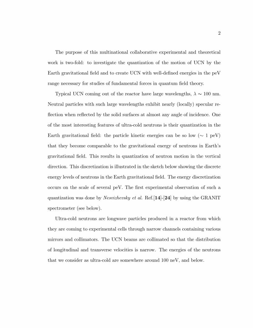
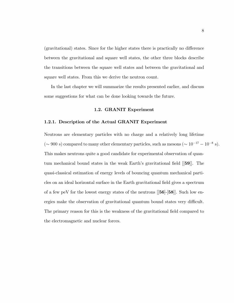
Figure 1.1. Sketch of the experimental cell with a neutron beam be-tween two plates. The neutrons bounce between the "rough" ceilingand "smooth" �oor. The neutrons with low vertical velocity, whichdo not reach the ceiling get to the detector.

The �rst experimental observation of quantum mechanical bound states of neu-

trons in the Earth�s gravitational �eld was made by Nesvizhevsky et al. in 2002

[[14]-[24]] after a series of experiments in high precision neutron gravitational spec-

trometry (GRANIT). The GRANIT experiment uses the fact that neutrons have

a relatively long lifetime by sending a collimated beam of UCN to the cell through

a long complicated waveguide with re�ective walls.

One can visualize in a simple way the observation of gravitationally induced

quantum states of UCN experiment. There is a collimated beam entering an

experimental cell (see Fig.1.1) consisting of a smooth "�oor" and a rough "ceiling".

More details of the GRANIT experiment will be discussed below [[14]-[24]].

More explicitly, we have a collimated beam of UCN with a large horizontal

velocity on the order of � (5� 15)m/s and a small vertical velocity of a few cm/s

10

propagating between two parallel horizontal sapphire mirrors. The bottom mirror

or "�oor" is made as close to perfect as possible. This ensures high probability of

specular re�ection for the bouncing neutrons. The upper mirror or "ceiling" has

a rough surface which is made rough by simply scratching the surface [[16],[61]] .

This rough mirror e¤ectively serves as a selector for the vertical component of the

velocity of the neutrons. The scattering by the rough ceiling makes the velocity

vector turn, which increases the vertical component of velocity and, therefore, the

probability of absorption of the neutrons by the wall material. When the vertical

velocity exceeds a certain critical value (� 4 m/s) as a result of scattering by

roughness, the neutrons penetrate the wall and disappear. Only the neutrons with

a low vertical velocity do not reach the rough ceiling, do not scatter and, therefore,

survive.

11

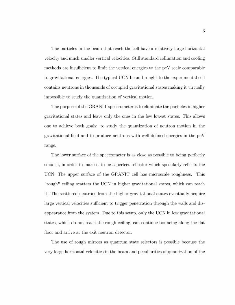
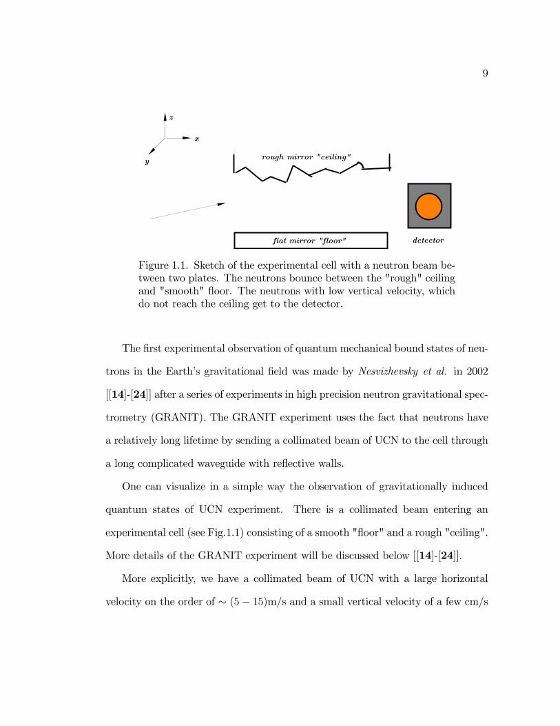
Figure 1.2. The GRANIT experiment: a more technical sketch ofthe experiment as a whole. The experimental cell is on the right.

The location of the waveguide is in the uppermost part of the spectrometer.

The reason for this is to isolate it from the e¤ects of external vibrations and from

electromagnetic �elds. The mirrors in the waveguide can be moved or even in-

terchanged. The positions can be adjusted vertically and horizontally depending

on what is needed in the experiment [[23]-[25]]. The con�guration that we use in

this thesis is the one shown in the �gure above in which the edges of the mirrors

are perfectly aligned and are of the order of 10cm long. The length represents the

minimum horizontal distance covered by the UCN inside the cell; the estimated

�ight time is about 20 ms. Additionally, the vertical separation between the mir-

rors (the width of the waveguide H) can be changed. The minimal width of the

waveguide is � 15 �m, which is comparable to the semi-classical amplitude of the

bounces of UCN in the ground state. The quantization of the UCN by the Earth�s

12

gravitational �eld translates into the quantization of the amplitudes of the bounces

from the �oor mirror.

Ideally, the neutron count at the location of the detector should be a step

function of the width H of the waveguide. The reason why we should have a

stepwise type function is because of the quantum size e¤ect. The quantum size

e¤ect occurs from a gravity-induced perpendicular quantization of the motion to

the bottom of the mirror, and leads to a split in the energy spectrum into mini-

bands. It is interesting to note that the sharpness of the quantum size e¤ect in

neutron count is related to the increase in roughness of amplitude l rather than

the correlation radius of roughness R (see below).

The roughness of the imperfections of the ceiling mixes the gravitational states

and broadens the energy levels. Below, we provide a quantitative description of

the roughness parameters governing the surface inhomogeneities.

1.2.2. Experimental Analysis of the Mirror Roughness

13

75mm 75mm 75mm 75mm

20mm

20mm

300mm

90mm

1

2

3

4

5

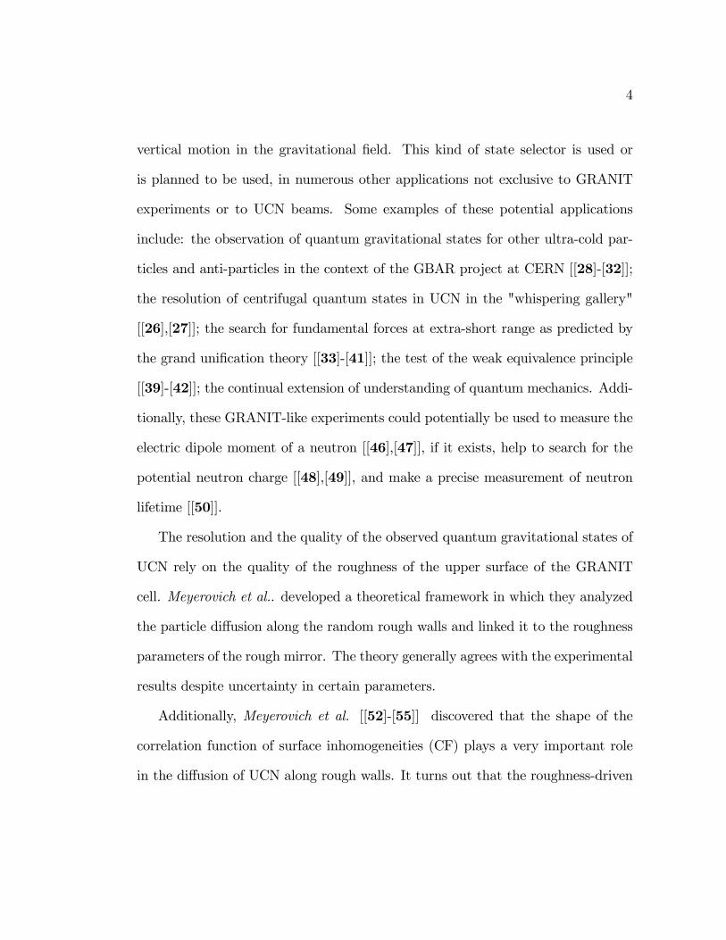
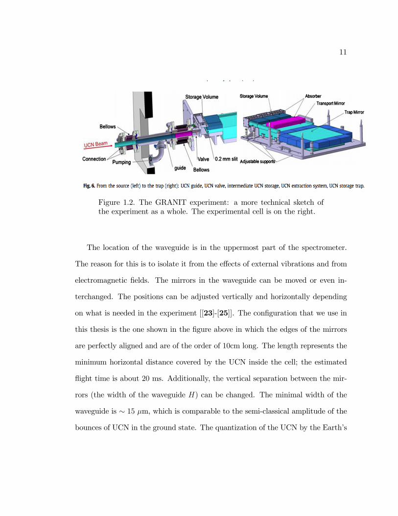
Figure 1.3. "Rough" ceiling mirror. The patches 1-5 represent thespots where the roughness has been measured using vertical scanninginterferometry.

One of the main goals of the GRANIT project is to continuously re�ne the

observation of the UCN spectrum. Since the �rst experiments in 2002, there have

been improvements made to the GRANIT spectrometer in order to reduce uncer-

tainties in the waveguide. Various parameters such as the correlation radius of

roughness R, amplitude of roughness l, and the oscillation frequency for neutrons

in the gravitational well � 0 have been adjusted and measured more accurately.

The latest improvement was the installation of a new large rough mirror on the

"ceiling".

The dimensions of the mirror are shown in the Fig.[1:3]. The UCN are propa-

gated along the 90mm long edge. The �ve square patches in the �gure represent

14

the areas where the mirror roughness has been measured. Each patch in the Figure

represents 0:504 � 0:504 mm2 and consists of a matrix of � 2500 � 2500 experi-

mental data points for which the surface position with respect to a mean reference

plane was measured. The surface roughness was measured using Vertical Scanning

Interferometry (VSI) technique. The surface was scanned using a light source that

splits into two coherent light beams. One of the two beams is sent towards a mirror

which is coupled with a di¤erent light beam that has been re�ected from a sample

(amplitude of roughness of 0.5 Å). The interference patterns are then analyzed

using a CCD camera and provide a surface pro�le. Unfortunately however, this

technique is not perfect. For example, the measurement fails if some peak is too

sharp and therefore the beam doesn�t re�ect back onto the detector. The experi-

mental data on the surface pro�le were analyzed numerically. It was determined

that the roughness correlation function most likely has an exponential shape. [9]

This technique though is more appropriate then other scanning techniques such

as the Atomic Force Spectroscopy. One of the reasons that VIS is better is that

the scanned surface is considerably larger than the correlation radius.

1.3. Notations and Dimensionless Variables

For the purpose of this work it is useful to introduce some uniform notations

for the calculations in both presence and absence of gravitational �eld. Some of

the parameters below will be used to make the equations dimensionless. We are

looking at the e¤ects of gravity on the transport of the UCN.

15

1. In this case it is useful to measure all lengths is units of:

(1.1) l0 =

�~

2m2g

�1=3� 5:87 �m;

This is the amplitude of the particle bouncing in the lowest quantum state in the

presence of the Earth gravitational �eld.

2. The energy scale is de�ned by:

(1.2) e0 = mgl0 � 0:602 peV;

This is the gravitational energy of the neutron in the ground state.

3. The velocity scale is de�ned by:

(1.3) v0 =p2gl0 =

~ml0

� 1:1� 10�2m/s:

4. The time scale is given by:

(1.4)1

� 0=

p2�

4m

~l20� 1149s�1:

This is roughly the frequency of bounces in the lowest state.

5.The width of the waveguide H in units of l0 is:

(1.5) h =H

l0:

16

6.The roughness correlation radius R expressed as a dimensionless variable is:

(1.6) r =R

l0:

7. Similarly, the amplitude of roughness l as a dimensionless variable is ex-

pressed as:

(1.7) � =l

l0:

8. The quantized energy levels Ej of the ultra-cold neutrons in the gravitational

well are given by:

(1.8) �j =Eje0:

9. The absorption threshold Uc of the mirror material is given by:

(1.9) uc =Uce0;

where Uc � 100 neV, and, therefore, uc � 1:4� 105.

10. The �ight time for the ultra-cold neutrons through the waveguide of the

length L is given by:

(1.10) �L =L

vx;

In experimental conditions �L � 2� 10�2s. In dimensionless units �L=� 0 � 26:

17

11. The neutron momenta are measured in units of:

(1.11) q0 =~l0:

1.4. Theoretical Background

1.4.1. Quantum Size E¤ect (QSE)

Ultra-cold neutrons (UCN) are longwave particles. We are looking at UCN in

narrow waveguides in which the width is comparable to the wavelength and the

motion across the waveguide is quantized. This QSE automatically discretizes the

initially continuous equations. This quantization turns out to be very fortuitous as

it helps in numerical calculations: if we were working with a continuous system, we

would need to discretize the problem anyway. QSE leads to a split of the energy

spectrum �(p) into a set of minibands �j(q) such that �(px;q) �!�j(q), where p

is the 3D momentum, and q is the 2D momentum in the plane of the surface.

More explicitly, an initially parabolic spectrum, �(p) = p2=2m becomes

(1.12) �j(q) =1

2m[(�~jH)2 + q2j ]

and the 2D momentum for miniband j becomes

(1.13) q2j = [2mE�(�~jH)2]

18

where E is the overall kinetic energy of particles, m is the mass of the neutrons,

H is the width of the channel.

In an ideal waveguide, the quantum levels are well de�ned and the states are

not mixing. Scattering by random surface inhomogeneities leads to inter- and

intraband transitions and eventually mixes and broadens the quantum states.

Sometimes, as in experiments performed at ILL (Grenoble), the waveguides,

or, more precisely, one of the neutron mirrors, are made rough on purpose.

1.4.2. Transport Equation

Studies on the e¤ect of random surface roughness on wave or particle scattering

describe the di¤usion �ows of UCN along a rough waveguide. Meyerovich et al.

[[1]-[8]] developed a rigorous theoretical framework of quantum transport theory in

system with random rough boundaries. This framework incorporates the boundary

scattering directly into the bulk transport equation. It includes the roughness

of the walls explicitly into the roughness-driven transition probabilities between

quantum states. The transport equation for distribution functions nj (q) in a

miniband j has the form

(1.14)dnjdt(q) = 2�

Xj0

ZWjj0(nj � nj0)�(�jq � �j0q0)

d2q0

(2�)2

19

where nj (q) is the distribution function of the particles, �jq is the energy spectrum,

q is the momentum in the plane parallel to the surface, and Wjj0 (q;q0) are the

scattering-driven probabilities of transitions between the states �j (q) and �j0 (q0).

The probabilities of direct transitions from the lowest states to the continuous

spectrum above the threshold Uc are negligible and such transitions can be disre-

garded. After integration over the energies, the transport equation acquires the

following form:

(1.15)@Nj

@t=m

2�

Xj0

Zd�Wjj0 (jqj � qj0j) (Nj0 �Nj)

where Nj is the number of neutrons in the state j, and � is the angle between qj

and qj0.

Our goal is to �nd the di¤usion coe¢ cient and the mean-free path, which is

proportional to the di¤usion coe¢ cient. After standard transformations (a more

detailed derivation can be found in the Appendices) the transport equation reduces

to a set of linear equations for �j (qj):

(1.16) Qj = �mXj0

�j0(qj0)

� jj0;

Here Qj is the momentum, the transition times � jj0 are given below by Eq.(1:24),

and �j is the �rst angular harmonic of the distribution function n(1)j = �j�(�� �F )

20

at q = qj, Ref.[[4],[5]]. The equations can be made dimensionless using

(1.17) qjq0 = �mXj0

e�j0�0e� jj0� 0which leads to

(1.18) qj = �m�0q0� 0

Xj0

e�j0e� jj0 ;where

(1.19) qj =Qjq0, e�j = �j

�0and e� jj0 = � jj0

� 0:

Finally, the dimensionless transport equation acquires the form:

(1.20) qj = �ml20~� 0

Xj0

f�j0(qj0)e� jj0 :

1.4.3. Transition Probabilities

The roughness-driven transition probabilities between quantized states have the

following form:

(1.21) Wjj0 = �j j(h)j2j j0(h)j2U2c

if the absorption threshold Uc is �nite. Alternatively,

(1.22) Wjj0 =1

4m2�j 0j(h)j2j 0j0(h)j2

21

when the absorption threshold Uc ! 1. Here j and j0 are the miniband indices,

� is the correlation function of surface homogeneities (see below), j(h) is the

wavefunction at the surface.

In the case of the square well potential this equation becomes the following :

(1.23) Wjj0(q;q0) =

~m2L2

�

��~jL

�2��~j0

L

�2:

The transitions times in the transport equation are directly related to the angular

harmonics of these transition probabilities as follows:

(1.24)2

� jj0= m

Xj00

h�jj0W

(0)jj00 � �j0j00W

(1)jj0

i1.4.3.1. Correlation Function of Roughness. The correlation function of sur-

face roughness (CF) is de�ned as:

(1.25) � (jsj) = h�(s1)�(s1 + s)i�A�1Z�(s1)�(s1 + s)ds1;

(1.26) � (jpj) =Zd2seiq:s� (jsj) = 2�

Z 1

0

� (s) J0 (qs) sds;

where � (jsj) is the exact pro�le of the wall and A is the area over which the

averaging is done. The mathematical form of the CF cannot be found theoretically

except in very few instances in which we have exactly solvable models of surface

22

roughness. It is usually assumed that the CF has the following general form:

(1.27) � (x) = l2' (x=R)

with some function ' (x=R), where l and R are the average amplitude and corre-

lation radius. However, nothing prevents the CF to acquire a more complicated

form, for example, with several correlation scales Rc. In calculations we assume

that we know the shape of the CF. The most commonly used correlation functions

have either the Gaussian

(1.28) � (s) = l2 exp(�s2=2R2);

(1.29) � (q) = 2�l2R2 exp��q2R2=2

�;

or exponential

(1.30) � (s) = l2 exp(�s=R)

(1.31) � (q) =2�l2R2

(1 + q2R2)3=2

forms. Sometimes people also use a CF with a power law shape. Here R is the

correlation radius of surface inhomogeneities., r = R=l0, and the dimensionless

23

amplitude is de�ned as � = l=l0. There are reasons to believe that the correlation

function in Grenoble experiments might be exponential, Ref.[[9]].

The angular harmonics of the Gaussian correlation function are

(1.32) �(0) = 4�l2R2he�qq

0�r2I0(qq0 � r2)

ie�r

2=2(q�q0)2

(1.33) �(1) = 4�l2R2he�qq

0�r2I1(qq0 � r2)

ie�r

2=2(q�q0)2

This means the transition probabilities W , Eq(1.23), are equal to Ref.[[4]]:

(1.34) W(0)jj0 =

}m2L2

��j

L

�2��j0

L

�24�l2R2

he�qq

0�r2I0(qq0 � r2)

ie�r

2=2(q�q0)2

(1.35) W(1)jj0 =

}m2L2

��j

L

�2��j0

L

�24�l2R2

he�qq

0�r2I1(qq0 � r2)

ie�r

2=2(q�q0)2

In dimensionless variables,

(1.36) w(0)jj0 =

8�r2p2�h

��j

h

�2��j0

h

�2 he�qq

0�r2I0(qq0 � r2)

ie�r2=2(q�q0)2

(1.37) w(1)jj0 =

8�r2p2�h

��j

h

�2��j0

h

�2 he�qq

0�r2I1(qq0 � r2)

ie�r2=2(q�q0)2

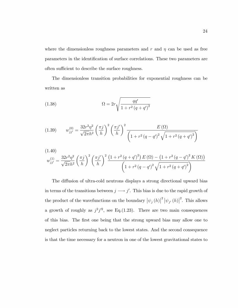
24

where the dimensionless roughness parameters and r and � can be used as free

parameters in the identi�cation of surface correlations. These two parameters are

often su¢ cient to describe the surface roughness.

The dimensionless transition probabilities for exponential roughness can be

written as

(1.38) = 2r

sqq0

1 + r2 (q + q0)2

(1.39) w(0)jj0 =

32r2�2p2�h2

��j

h

�2��j0

h

�2E ()�

1 + r2 (q � q0)2q1 + r2 (q + q0)2

�(1.40)

w(1)jj0 =

32r2�2p2�h2

��j

h

�2��j0

h

�2 �1 + r2 (q + q0)2�E ()�

�1 + r2 (q � q0)2K ()

��1 + r2 (q � q0)2

q1 + r2 (q + q0)2

�The di¤usion of ultra-cold neutrons displays a strong directional upward bias

in terms of the transitions between j �! j0. This bias is due to the rapid growth of

the product of the wavefunctions on the boundary�� j (h)��2 �� j0 (h)��2. This allows

a growth of roughly as j2j02, see Eq.(1.23). There are two main consequences

of this bias. The �rst one being that the strong upward bias may allow one to

neglect particles returning back to the lowest states. And the second consequence

is that the time necessary for a neutron in one of the lowest gravitational states to

25

di¤use upward towards the absorption barrier is spent almost entirely on the �rst

transition.

In the next chapter we will examine more closely the process of di¤usion, and

expand upon and develop a more detailed theoretical approach.

CHAPTER 2

Di¤usion Coe¢ cient and Mean Free Path in a Rough

Waveguide

2.1. Introductory Comments

Let us examine the transition probabilities which for the sake of the numerical

computations need to be made dimensionless. Furthermore, we are going to de-

�ne some parameters used in the numerical computations. In the context of our

research, we want to look at both Gaussian and exponential roughness associated

with the correlation functions �, which together with the wavefunctions at the wall

form the transition probabilities, Eq.(1:36)-Eq.(1:37) , and Eq.(1:39)- Eq.(1:40).

The transition probabilities are proportional to the square of the amplitude of

roughness �. Therefore, the scaling of the results with the roughness amplitude �

is trivial and in most of the computations we simply assume � = 1. The scaling of

the results with the correlation radius r = R=l0 is complicated and is not known

beforehand. One of our main goals is to �nd out the dependence of the di¤usion

parameters on r.

In relevant experiments the width of the channels leading to the cell is H = 50

�m, and the particle energy is E = 150 neV; this makes h = 8:52, and e = 2:49�105.

The highest occupied quantum level jmax satis�es the inequality,

26

27

(2.1) e� �2j2maxh2

� 0

Solving for jmax we get

(2.2) jmax =

reh2

�2= 1352

which means that the transport equation in this case reduces to a set of 1352

coupled equations.

2.2. The Di¤usion Coe¢ cient

The main purpose of this section of the work was to �nd the di¤usion coe¢ cient

and the mean free path for UCN in rough channels. We are trying to examine how

the di¤usion coe¢ cient changes under di¤erent conditions. More explicitly, we

are interested in its dependence on r. Di¤usion is a process that originates from

random motion of particles when there is a net �ow from one region to another. As

a result, in our case, in the presence of a concentration gradient r� the di¤usion

equation reduces to

(2.3)1

Smr� �Qj = �

Xj0

�j0

� jj0;

28

where � is the particle density. Its concentration gradient r� is a simple scal-

ing parameter, which, in the end, cancels out from the equation for the di¤usion

coe¢ cient. After this cancellation, the di¤usion coe¢ cient D becomes

(2.4) D = � 1m

Xj0

Qj0�j0

The dimensionless di¤usion coe¢ cient

d = D=d0 =Xj0

dj;

dj = qj e�j;d0 = ~=m = 6:3 � 10�8m=s2:

The dimensionless distributions e�j = �j=l0 are obtained from numerically solving

the transport equation.

2.3. Mean Free Path

We also want to calculate the particle mean-free path (MFP) in a rough

waveguide. The mean free path in very basic terms is the average distance traveled

between collisions. Here we de�ne it with respect to the di¤usion coe¢ cient as

(2.5) L =D=v;

29

where v is the velocity. The dimensionless velocity

ev = 1

v0

r2e0m

pe

where v0 = 1:5 � 10�2m=s. The dimensionless mean free path ` = L=l0,

` =2d0l0v0

dev = 2d0l0

rm

2e0

dpe:

As one can clearly see the MFP is intimately related to the di¤usion coe¢ cient.

2.4. Numerical Results

Before presenting the results, let us summarize the dimensionless equations

from above. The transport equation ,

(2.6) qj = �ml20~� 0

Xj0

e�j0(qj0)e� jj0 ;

contains the transition times

(2.7)2e� jj0 = m

Xj00

h�jj0w

(0)jj00 � �j0j00w

(1)jj0

i:

The dimensionless harmonics of the transition probabilities for the exponential and

Gaussian roughness correlators are given in explicit detail in the Appendix A.

For the overall and "partial" di¤usion coe¢ cients d and dj the dimensionless

equations are as follows

30

d = D=d0 =Xj0

dj;

dj = qje�j:Finally, the MFP is

(2.8) ` =2d0l0

rm

2e0

dpe:

Using the dimensionless equations for the transition probabilities from the pre-

vious section, we are now able to perform computations to get the di¤usion coef-

�cient and MFP. The computations are done in Mathematica, where we use the

function LinearSolve [m,b] which �nds an x that solves the matrix equation

m.x==b. to get the � values. This is the part of the program that is compu-

tationally the longest as it essentially solves a system of 1352 linear equations

with complicated coe¢ cients and varied parameters. After that, we calculate the

dimensionless partial di¤usion coe¢ cients,

(2.9) dj = e�jqjand sum them to get the overall di¤usion coe¢ cient. We easily get the MFP by

by using Eq. (2:8).

31

In our numerical simulations we were using a �xed channel width h = 8:52

(the number given to us by GRANIT experimentalists) and were changing the

correlation radius of surface inhomogeneities r. Before we go into the descriptions

of the various curves, it is important to note that all the curves for d (r) are

expected to have the minimum at, approximately, qr s 1 for both Gaussian and

exponential surface correlators. The experimental value of the particle energy is

E = 150 neV, i.e., e t 2:5 � 105, which makes q1 t 500. This means that the

minimum corresponds to very small values of r, r s 0:002, and cannot be resolved

on many of the curves below. The explanation for this minimum is rather simple.

The scattering by surface inhomogeneities is most e¤ective at qr s 1 leading to a

minimum in the di¤usion coe¢ cient d (r). There could be several small minima at

qjr s 1 but all corresponding values of r are small. For this reason, below we will

show mostly the results for noticeably larger values of r, i.e., to the right of the

minimum.

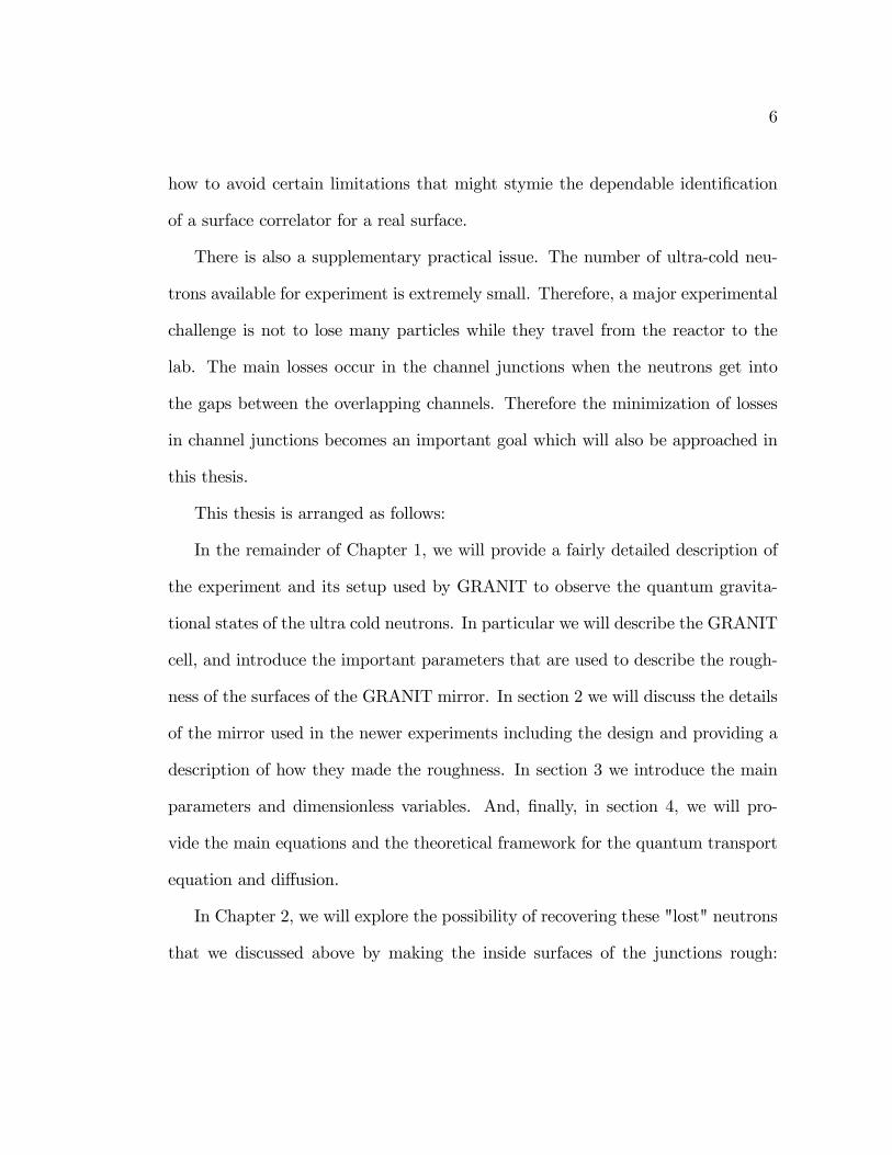
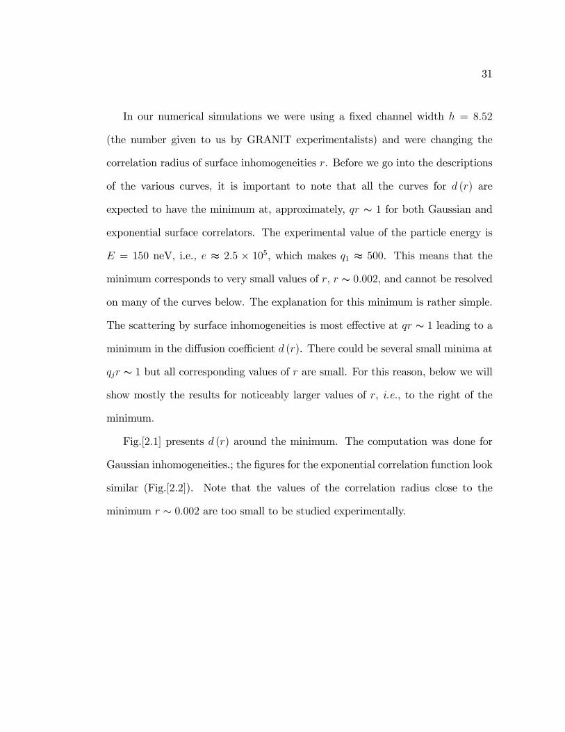
Fig.[2:1] presents d (r) around the minimum. The computation was done for

Gaussian inhomogeneities.; the �gures for the exponential correlation function look

similar (Fig.[2:2]). Note that the values of the correlation radius close to the

minimum r � 0:002 are too small to be studied experimentally.

32

r0.000 0.002 0.004 0.006 0.008 0.0100

d(r) 106

1

2

3

4

5

Figure 2.1. Minima of the di¤usion coe¢ cient d(r) as a function ofthe correlation radius for the Gaussian inhomogeneities. The di¤u-sion coe¢ cient starts growing again at larger r.

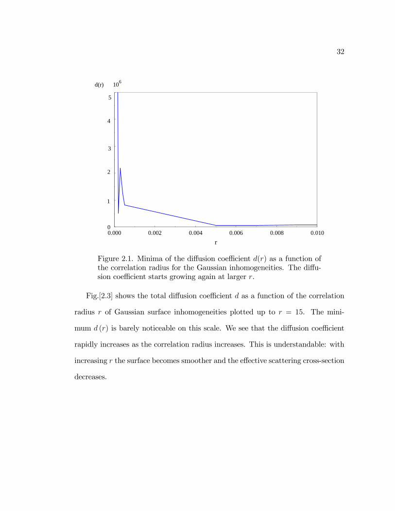
Fig.[2:3] shows the total di¤usion coe¢ cient d as a function of the correlation

radius r of Gaussian surface inhomogeneities plotted up to r = 15. The mini-

mum d (r) is barely noticeable on this scale. We see that the di¤usion coe¢ cient

rapidly increases as the correlation radius increases. This is understandable: with

increasing r the surface becomes smoother and the e¤ective scattering cross-section

decreases.

33

r0 5 10 15

0

d(r) 108

20

15

10

5

Figure 2.2. Di¤usion coe¢ cient d (r) for the Gaussian surface corre-lator over large range of r. The minima in d (r) cannot be resolvedon this scale.

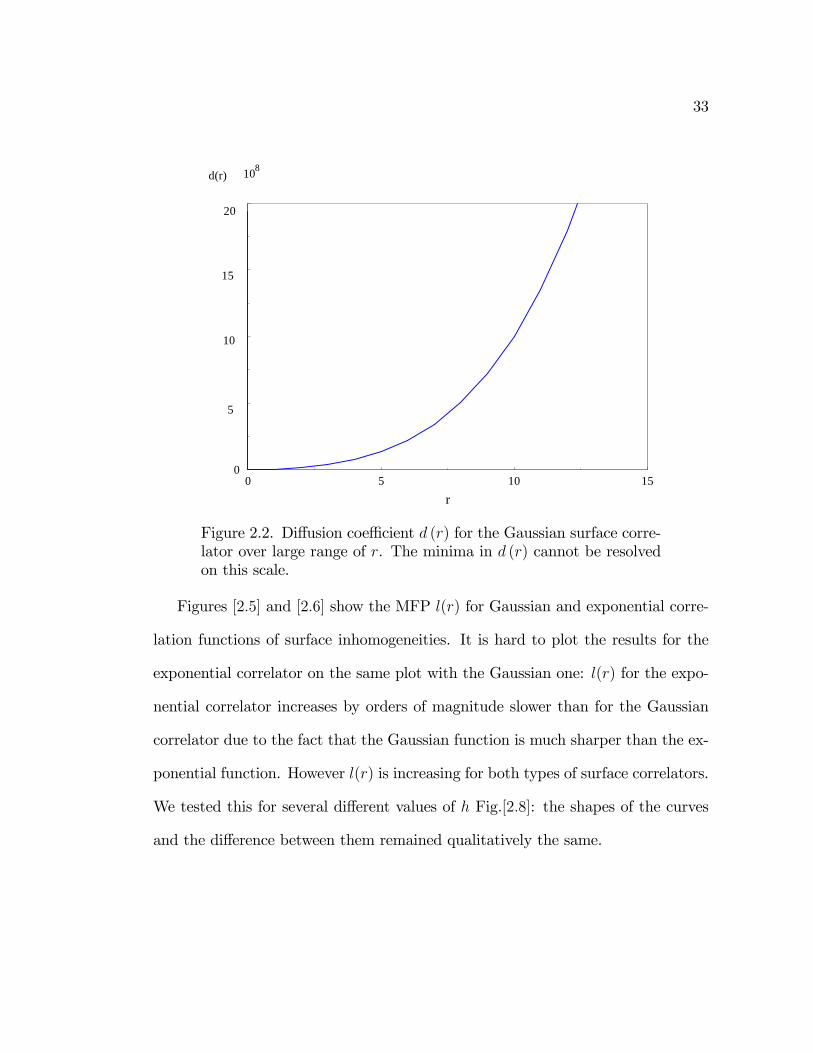
Figures [2:5] and [2:6] show the MFP l(r) for Gaussian and exponential corre-

lation functions of surface inhomogeneities. It is hard to plot the results for the

exponential correlator on the same plot with the Gaussian one: l(r) for the expo-

nential correlator increases by orders of magnitude slower than for the Gaussian

correlator due to the fact that the Gaussian function is much sharper than the ex-

ponential function. However l(r) is increasing for both types of surface correlators.

We tested this for several di¤erent values of h Fig.[2:8]: the shapes of the curves

and the di¤erence between them remained qualitatively the same.

34

r0.0 0.1 0.1 0.2 0.2 0.3 0.3 0.4 0.4 0.5 0.5

0

d(r)

x 104

5

10

15

20

Figure 2.3. The next �gure (Fig.[2:4]) shows the di¤usion coe¢ cientfor the exponential correlation function of surface roughness.

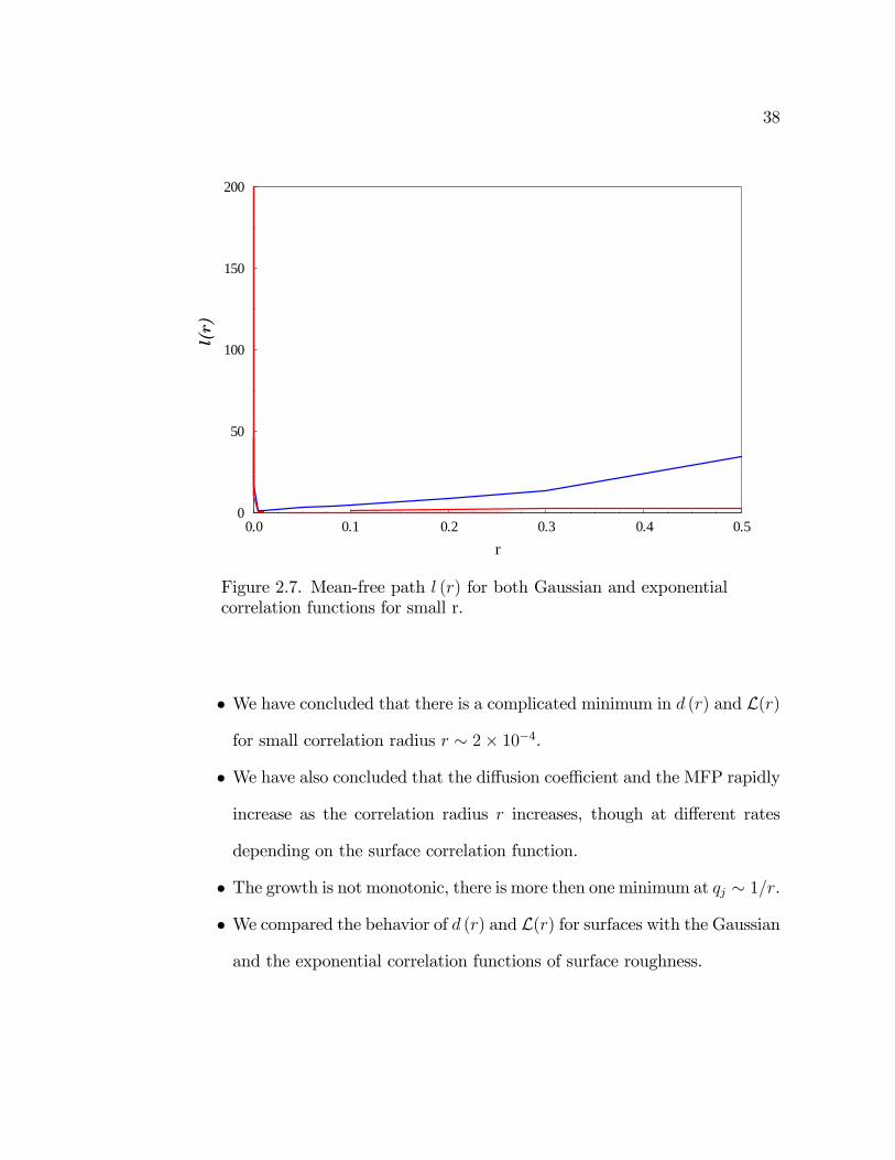
Figure [2:7] compares the MFP for Gaussian and exponential surface correlation

functions for a small range of r.

35

r0 10 20 30 40 50 60

0

d(r)

2

4

6

8

10

x106

Figure 2.4. Di¤usion for the surface inhomogeneities with the expo-nential correlation function over large range of r.

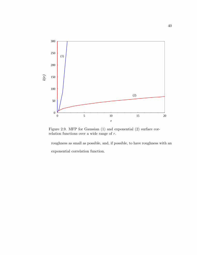
Similarly, Figure [2:9] illustrates the fact that the MFP l(r) for the Gaussian

and exponential correlation functions is more or less the same up to r � 2. Starting

from this point the result for the Gaussian correlation function increases much

faster than for the exponential function. We think the reason is that the Gaussian

function decays much faster than the exponential which manifests itself at large

values of r.

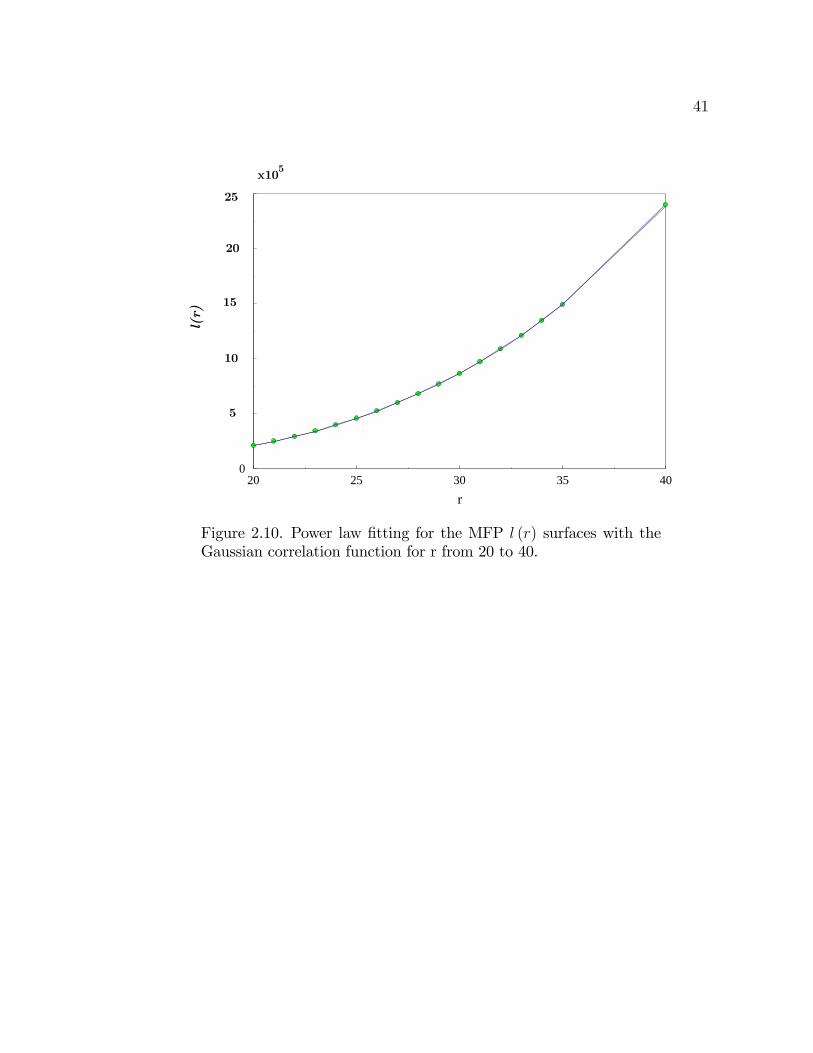
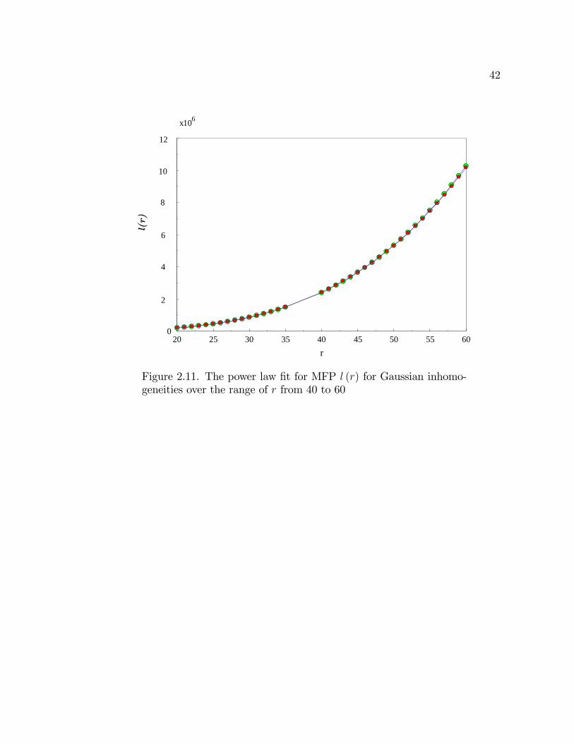
The next few curves, Figures.[2:10� 2:12], illustrate �tting of the MFP curves

for l(r) by the power law functions. If we look at the Gaussian correlation function

36

r0 10 20 30 40 50 60 70 80

l(r)

0

5

10

15

20

25

30

Figure 2.5. Mean free path l (r) for the surface with Gaussian rough-ness over wider range of r.

d (r) in the ranges of r from 1 to 20 we get a pretty good �t using the power function

d (r) / rp with the index p = 2:7.

37

r0 10 20 30 40 50 60 70 80

l(r)

0

500

1000

1500

2000

Figure 2.6. Mean free path for the surface with exponential rough-ness over wider range of r.

Looking at d (r) in the range of r s 20 � 60, we also get a good �t using the

power law, with the power p = 3:5. Looking at the exponential correlation function

d (r) in the ranges of r from 1� 40, we see that we get a good �t using the power

law, with the power p = 2:95.

2.5. Conclusions

� We calculated the di¤usion coe¢ cient and the mean free path for ultra-

cold neutrons in narrow channels with random rough walls.

38

r0.0 0.1 0.2 0.3 0.4 0.5

l(r)

0

50

100

150

200

Figure 2.7. Mean-free path l (r) for both Gaussian and exponentialcorrelation functions for small r.

� We have concluded that there is a complicated minimum in d (r) and L(r)

for small correlation radius r � 2� 10�4.

� We have also concluded that the di¤usion coe¢ cient and the MFP rapidly

increase as the correlation radius r increases, though at di¤erent rates

depending on the surface correlation function.

� The growth is not monotonic, there is more then one minimum at qj � 1=r.

� We compared the behavior of d (r) and L(r) for surfaces with the Gaussian

and the exponential correlation functions of surface roughness.

39

r0 10 20 30 40 50 60 70 80

l(r)

0

x107

1

2

3

4

Figure 2.8. MFP for Gaussian correlation function for various chan-nel widths h = 16, 8, 4.

� The function d (r) behaves roughly as r3, though the exponent slightly

drifts with r. This seems to be an important conclusion, though we do

not have an explanation for this functional dependence.

� The computations were done for realistic values of the channel width h =

8:52. At di¤erent values of h the results were qualitatively the same.

� The growth of d (r) and L(r) for the Gaussian surface correlation function

is much slower than for the exponential correlation function.

� If one wants to e¤ectively turn back the neutrons which got into the gaps

in the channel junctions, one should make the correlation radius of surface

40

r0 5 10 15 20

l(r)

0

50

100

150

200

250

300

(2)

(1)

Figure 2.9. MFP for Gaussian (1) and exponential (2) surface cor-relation functions over a wide range of r.

roughness as small as possible, and, if possible, to have roughness with an

exponential correlation function.

41

r20 25 30 35 40

l(r)

0

5

10

15

20

25

x105

Figure 2.10. Power law �tting for the MFP l (r) surfaces with theGaussian correlation function for r from 20 to 40.

42

r20 25 30 35 40 45 50 55 60

l(r)

0

x106

2

4

6

8

10

12

Figure 2.11. The power law �t for MFP l (r) for Gaussian inhomo-geneities over the range of r from 40 to 60

43

0 5 10 15 20 25 300

500000

1000000

1500000

2000000

2500000

d(r)

r

Figure 2.12. Power law �t for d (r) the exponential surface correla-tion function over a large range of r.

CHAPTER 3

Neutron Beams between Absorbing Rough Walls: Square

Well Approximation

3.1. Description of Problem

In this Chapter we deal with a slightly di¤erent UCN di¤usion problem which

is more directly related to the GRANIT experiments in the ILL, Grenoble. In

experiments the UCNs travel between rough absorbing walls and the number of

UCNs exiting the cell is measured as a function of the distance between the walls.

We start from discussing the case without gravity because it is simple and will

serve as a good reference point. By comparing numerical results obtained with

and without gravity we will understand what part of the experimental results

should be directly attributed to the Earth�s gravitational �eld.

The neutrons in the cell are passing between the two mirrors, the perfectly

smooth bottom mirror ("�oor"), and the randomly rough upper mirror ("ceiling").

44

45

z

x

y rough mirror "ceiling"

flat mirror "floor" detector

Figure 3.1. Sketch of neutron beam entering the experimental cell:the neutrons pass between rough "ceiling" and smooth "�oor".

The UCNs entering the cell have a large horizontal velocity (� 5� 15 m/s)

and very small vertical velocities. When the neutrons scatter o¤ the rough ceiling,

the velocity vector with large horizontal component turns thus increasing the ver-

tical component of the velocity. If the vertical velocity exceeds a certain velocity

threshold (the critical velocity is � 4 m=s), the neutrons penetrate the wall, are

absorbed, and do not reach the detector. The neutrons which manage to make

it through the cell without reaching the critical vertical velocity are not absorbed

and reach the neutron detector at the end of the cell.

The parameter that can be easily manipulated in experiment (and, of course,

in calculations) is the cell width H. In computations we look at about 1000 values

of dimensionless h = H=l0 between 0 and 9. This problem di¤ers from the setup

mentioned in the section above where we are studying the di¤usion coe¢ cient d (r)

46

and the MFP not only in the fact that we are now measuring the exit neutron

count, but also in the fact that we are now dealing with absorbing walls and

time-dependent numbers of neutrons. Again, the main di¤erence with regard to

the previous chapter on di¤usion is that previously we were letting the neutrons

just bounce around without disappearing (they decay naturally at around 900 s).

Now the neutrons disappear forever as the component of the velocity normal to

the wall reaches a threshold valuep2mUc and the number of neutrons becomes

time-dependent as well.

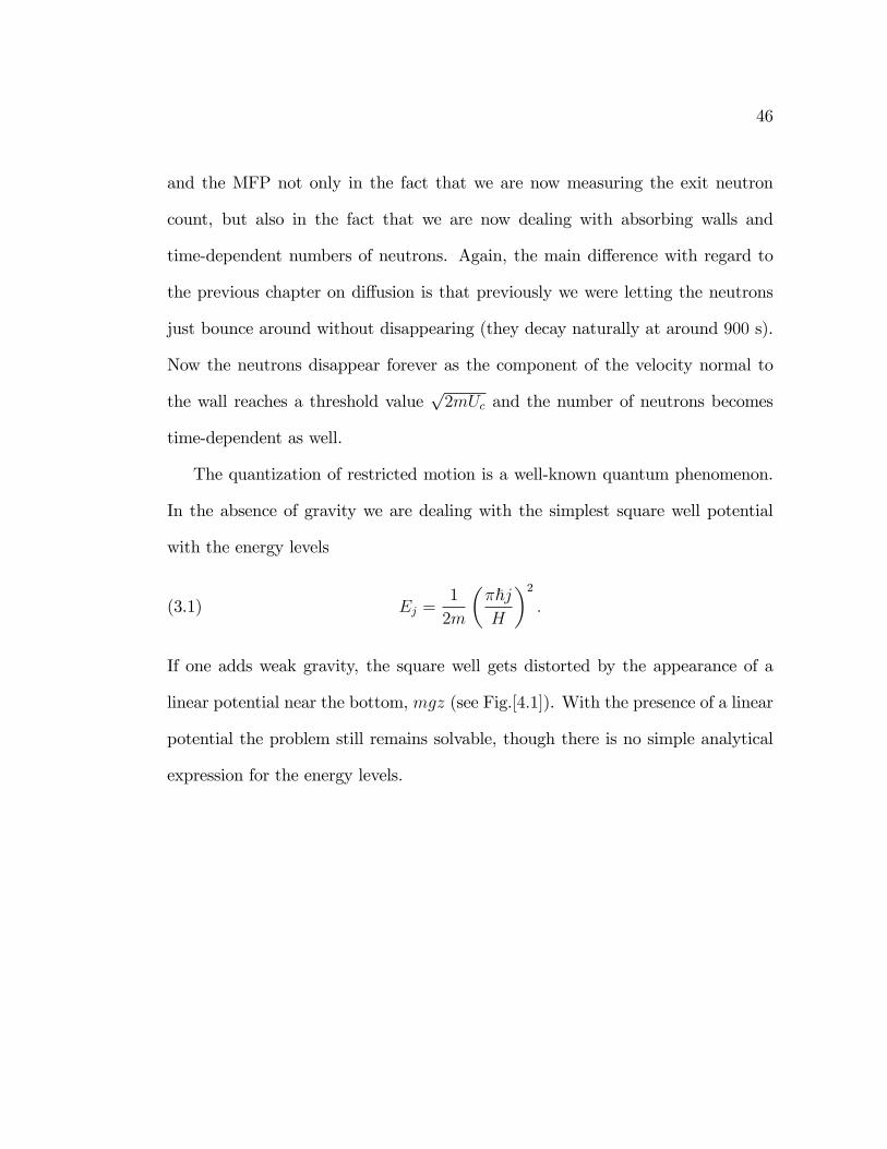
The quantization of restricted motion is a well-known quantum phenomenon.

In the absence of gravity we are dealing with the simplest square well potential

with the energy levels

(3.1) Ej =1

2m

��~jH

�2:

If one adds weak gravity, the square well gets distorted by the appearance of a

linear potential near the bottom, mgz (see Fig.[4:1]). With the presence of a linear

potential the problem still remains solvable, though there is no simple analytical

expression for the energy levels.

47

n=1

n=2

n=3

n=4

n=5

Figure 3.2. Square well levels.

To recap from the experiment brie�y, we are dealing with a collimated beam

being sent between two horizontal solid plates (one which is an almost ideal mirror

and the other is rough) that are at a distance of several micrometers apart. We

know that the neutrons hitting the wall with the normal velocity above 4 m/s get

absorbed by the plates. Below this threshold velocity the neutrons get re�ected.

The re�ection is specular locally.

First, we will neglect the presence of gravity. The e¤ects of gravity will be

introduced later, in the next chapter.

48

3.2. Wavefunction for the Square Well

We start by introducing the equation for the wavefunction on the wall in the

square well,

(3.2) j (H) =

r2

Hsin

��j~Hqj

�

where H is the width of the waveguide. Below we will use the same dimensionless

variables as in the previous chapter.

To determine the roughness-driven transition probabilities, Eq.(3:7), we need

the value of the square of the wavefunction at the upper wall. The equations that

we are using can be written in terms of bj Eq.(3:3) and since it is the quantity that

has been used throughout the years in the papers by Meyerovich et al, Ref.[[1]-[8]]

it is also the notation that we will be using from here on out in this thesis. Hence,

we de�ne the bj in dimensionless units as follows,

(3.3) bj (H) = 105 l0

2 (H)

2:

In the case of the square well this reduces to

(3.4) bj = 105 �jh uc

;

49

where �j is de�ned as

(3.5) �j =

��j

h

�2:

The values of bj�s in the gravitational potential we will get from the Airy functions,

which will be discussed more in the next section. The constant 105 is here merely

as a scaling factor to avoid dealing with very small numbers.

50

0 2 4 6 8 100

500

1000

1500

2000

2500

3000

bj(h)

h

Figure 3.3. Coe¢ cients bj(h) Ref[3.3] as a function of the width ofthe channel h for the square well.

In Fig.[3:3] we see the values of wavefunctions squared on the wall as a function

of the width of the channel h.

3.3. Transition Probabilities and Neutron Count

As mentioned above, we are dealing with the same set of transport equations

as in the previous Chapter of di¤usion and mean-free path. Here again, we start

51

with the transport equation,

(3.6)@Nj

@t=m

2�

Zd� Wjj0 (jqj � qj0j) (Nj0 �Nj) :

In this section we are looking only at the exponential correlation function of the

surface inhomogeneities and are not interested in the potential Gaussian correla-

tions. The reason for this is that recent analysis of the surface roughness of the

new "rough" mirror have led us to believe that the surface roughness is exponen-

tial rather than Gaussian Ref.[9] We therefore use the transition probabilities with

the exponential correlation function. Since we previously introduced the transition

probabilities, we will write them directly in dimensionless variables,

(3.7) w(0)jj0 =

32r2�2p2�h2

��j

h

�2��j0

h

�2E ()�

1 + r2 (q � q0)2q1 + r2 (q + q0)2

�(3.8)

w(1)jj0 =

32r2�2p2�h2

��j

h

�2��j0

h

�2 �1 + r2 (q + q0)2�E ()�

�1 + r2 (q � q0)2

�K ()�

1 + r2 (q � q0)2q1 + r2 (q + q0)2

� ;

where

(3.9) = 2r

sqq0�

1 + r2 (q + q0)2� :

and E () and K () are elliptical integrals.

52

As above we use the transition probabilities to get the dimensionless transition

frequencies ��1jj0 ,

(3.10)1

� jj0=Xj00

h�jj0w

(0)jj00 � �j0j00w

(1)jj00

iwe can now write the neutron exit count in terms of these relaxation times in a

simple form

(3.11)Ne (L)

N0=Xjj0

exp

�� tL� j

�;

where tL is the time of �ight of the UCN between the mirrors and � j are the

eigenvalues of Eq: (3:10).

3.4. Numerical Results

Initially, we want to start o¤ by de�ning and discussing the parameter that we

introduce, S1. The S1 parameter is a cuto¤ parameter. If we were to numerically

solve the above equations for the whole system, we would be solving more than 103

coupled linear equations with complicated coe¢ cients. Solving a system of that

many equations is computationally very expensive time-wise even with modern

computers, as each value takes approximately 30 min, and we do 900 iterations

over values of h from 9 to 1 for each r. Therefore, we wanted to examine if

there were a reasonable cuto¤, which would keep enough equations to not lose

much accuracy in the calculations, while also being much less expensive time-wise

53

computationally. To identify the S1 cuto¤, we simply run the computations using

more and more equations until we see that there is a saturation in the results. The

saturation point becomes our cuto¤point. We de�ne that parameter as S1: In this

section we are presenting some of our numerical results.

As we see in the �gures below, Fig.[3.4]-Fig.[3:9], we are plotting the number of

neutrons exiting the waveguide as a function of the size of the matrix S1. As one

can see from all these �gures presenting the exit neutron count as a function of S1

for various values of r and h, in all the cases S1 � 300 can serve as a good cuto¤

parameter. From this point onward, we choose in all computations S1 � 300 and

just occasionally check the results for larger matrices.

As a next step, we compute the dependence of the exit neutron count Ne on r

and h. The following �gures showNe (h) for r = 1; 5; 10; 30. The data in the �gures

show that, in principle, the neutron count is very sensitive to both r and h. The

common feature is that the exit neutron count is always extremely small except for

very small values of h and large values of r. For practical purposes this means that

taking into account the small number of ultra-cold neutrons entering the waveguide,

we should not expect any neutrons exiting at all. The obvious conclusion is that

the existence of neutrons exiting the cell in the Grenoble experiments is due only to

the Earth gravitational �eld (see the next section). Though this gravitational �eld

is extremely weak, without it the neutron count would have shown zero neutrons

exiting the cell with rough walls.

54

100 200 300 400 5005.9375

5.9380

5.9385

5.9390

5.9395

Nex10­39

S1

h = 8

Figure 3.4. Ne as a function of the cuto¤ parameter S1 for h = 8and r = 0:65. Here we can see the initial increase.

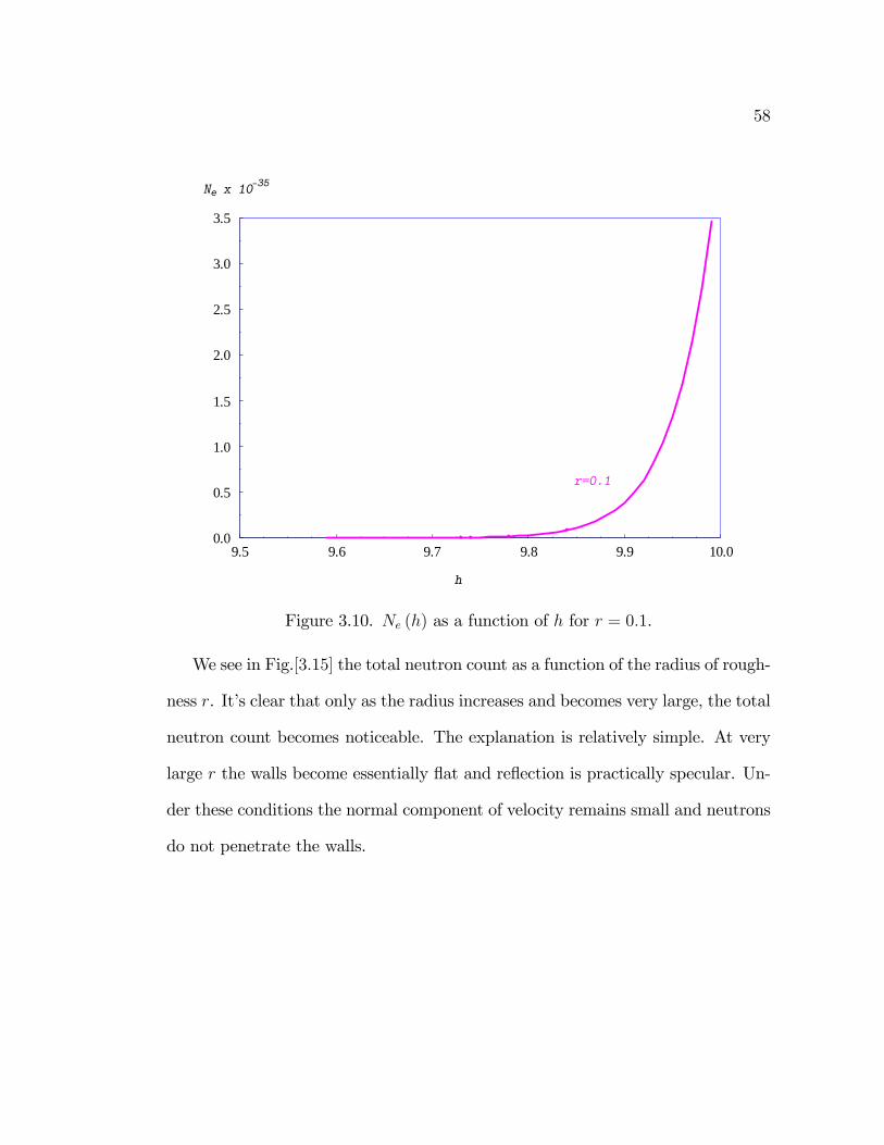
As we can see from the plot, Fig.[3:10], representing the total neutron count as

a function of h for very small r = 0:1, already at large h the number of surviving

neutrons goes to zero almost immediately when we have such a small correlation

radius.

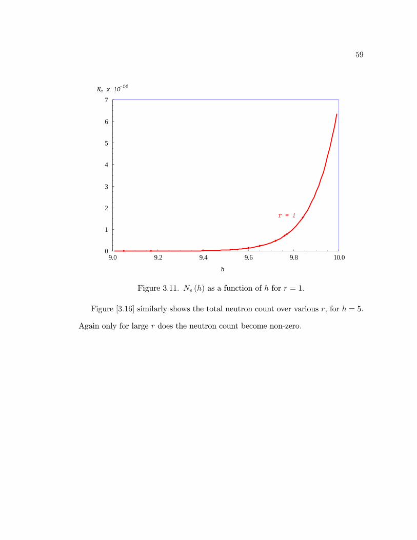
For r = 1, Fig.[3:11], we see that the depletion of the total neutron count to

zero is slightly less rapid, though it also goes to zero very quickly around h = 9:4.

Though again, if one pays attention to the Ne(h) axis, we see that the number

starts from what is essentially zero to begin with.

55

100 200 300 400 5005.937

5.938

5.939

5.940

5.941

5.942

5.943

5.944

5.945

Nex10­39

S1

h = 8

Figure 3.5. Neutron count as a function of the size of the matrix S1for h = 8 and r = 0:65. We can see how it saturates nicely, at aboutS1 = 300. In this plot we are looking at Ne over a larger scale.

0 100 200 300 400 500 6001.668

1.669

1.670

1.671

1.672

1.673

1.674

S1

Ne x 10­128

h=5

Figure 3.6. Ne as a function of the size of the matrix S1 for h = 5and r = 0:65. We are looking at Ne closer scale, so that we can seethe inital increase and gradual saturation.

56

0 100 200 300 400 500 6001.665

1.670

1.675

1.680

1.685

1.690

S1

Ne x 10­128

h=5

Figure 3.7. Saturation of the neutron count as a function of the sizeof the matrix S1, for h = 5 and r = 0:65.

50 100 150 200 250 300 350 4001.530

1.532

1.534

1.536

1.538

1.540

h=3

S1

Ne x10­589

Figure 3.8. Ne as a function of the matrix size S1 for h = 3 andr = 0:65. We are looking at Ne closer scale, so that we can see theinital increase and gradual saturation.

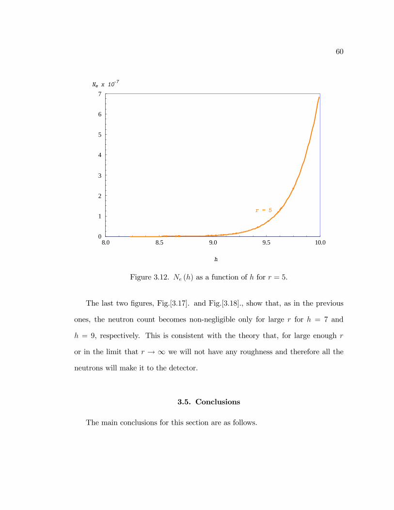
The results for the total neutron count for r = 5, Fig.[3:12] are consistent with

the above results, though now the neutron count goes to zero for the width size of

h = 8:7 .

57

0 50 100 150 200 250 300 350 400

1.535

1.540

1.545

1.550

1.555

1.560

h=3

S1

N(t)x10­589

Figure 3.9. Neutron count as a function of the cuto¤ parameter S1and r = 0:65 for h = 3.

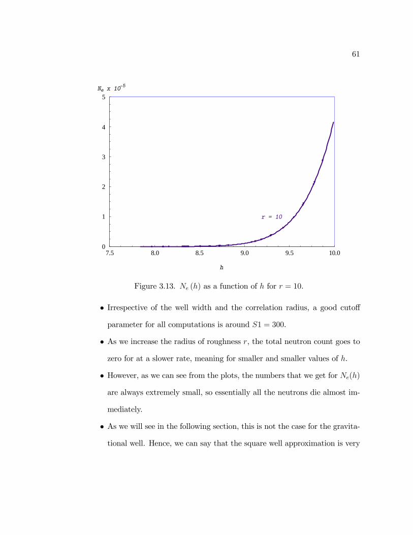
In the last two plots, we are computing the total neutron count Ne (h) over

the full range of h for r = 10 (Fig.[3:13]) and r = 30 (Fig.[3:14]). As with all the

results that we presented previously for varying r, we observe again that as we

increase the radius of roughness the total neutron count goes to zero slower which

here means at a smaller width size h.

58

9.5 9.6 9.7 9.8 9.9 10.00.0

0.5

1.0

1.5

2.0

2.5

3.0

3.5

r=0.1

Ne x 10­35

h

Figure 3.10. Ne (h) as a function of h for r = 0:1.

We see in Fig.[3:15] the total neutron count as a function of the radius of rough-

ness r. It�s clear that only as the radius increases and becomes very large, the total

neutron count becomes noticeable. The explanation is relatively simple. At very

large r the walls become essentially �at and re�ection is practically specular. Un-

der these conditions the normal component of velocity remains small and neutrons

do not penetrate the walls.

59

9.0 9.2 9.4 9.6 9.8 10.00

1

2

3

4

5

6

7

r = 1

h

Ne x 10­14

Figure 3.11. Ne (h) as a function of h for r = 1.

Figure [3:16] similarly shows the total neutron count over various r, for h = 5.

Again only for large r does the neutron count become non-zero.

60

8.0 8.5 9.0 9.5 10.00

1

2

3

4

5

6

7

r = 5

Ne x 10­7

h

Figure 3.12. Ne (h) as a function of h for r = 5.

The last two �gures, Fig.[3:17]. and Fig.[3:18]., show that, as in the previous

ones, the neutron count becomes non-negligible only for large r for h = 7 and

h = 9, respectively. This is consistent with the theory that, for large enough r

or in the limit that r ! 1 we will not have any roughness and therefore all the

neutrons will make it to the detector.

3.5. Conclusions

The main conclusions for this section are as follows.

61

7.5 8.0 8.5 9.0 9.5 10.00

1

2

3

4

5

r = 10

Ne x 10­5

h

Figure 3.13. Ne (h) as a function of h for r = 10.

� Irrespective of the well width and the correlation radius, a good cuto¤

parameter for all computations is around S1 = 300.

� As we increase the radius of roughness r, the total neutron count goes to

zero for at a slower rate, meaning for smaller and smaller values of h.

� However, as we can see from the plots, the numbers that we get for Ne(h)

are always extremely small, so essentially all the neutrons die almost im-

mediately.

� As we will see in the following section, this is not the case for the gravita-

tional well. Hence, we can say that the square well approximation is very

62

6.5 7.0 7.5 8.0 8.5 9.0 9.5 10.00.0

0.5

1.0

1.5

2.0

2.5

3.0

3.5

h

Ne x 10­3

r = 30

Figure 3.14. Ne (h) as a function of h for r = 30.

poor for this particular problem: though the weak Earth gravitational

�eld introduces only a small distortion near the bottom of the potential

well, its e¤ect on the neutron survival rate is very profound.

63

0 40 80 120 160

7

Ne(r) x 10­18

h=3

6

5

4

3

2

1

Figure 3.15. Total neutron count Ne as a function of di¤erent corre-lation radii r for small well width h = 3.

64

0 40 80 120 1600.00000

0.00005

0.00010

0.00015

0.00020

0.00025

Ne(r)

r

h=5

Figure 3.16. Total neutron count Ne as a function of di¤erent corre-lation radii r for well width h = 5.

65

0 40 80 120 1600.000

0.005

0.010

0.015

0.020

h=7

r

Ne(r)

Figure 3.17. Total neutron count Ne as a function of di¤erent corre-lation radii r for well width h = 7.

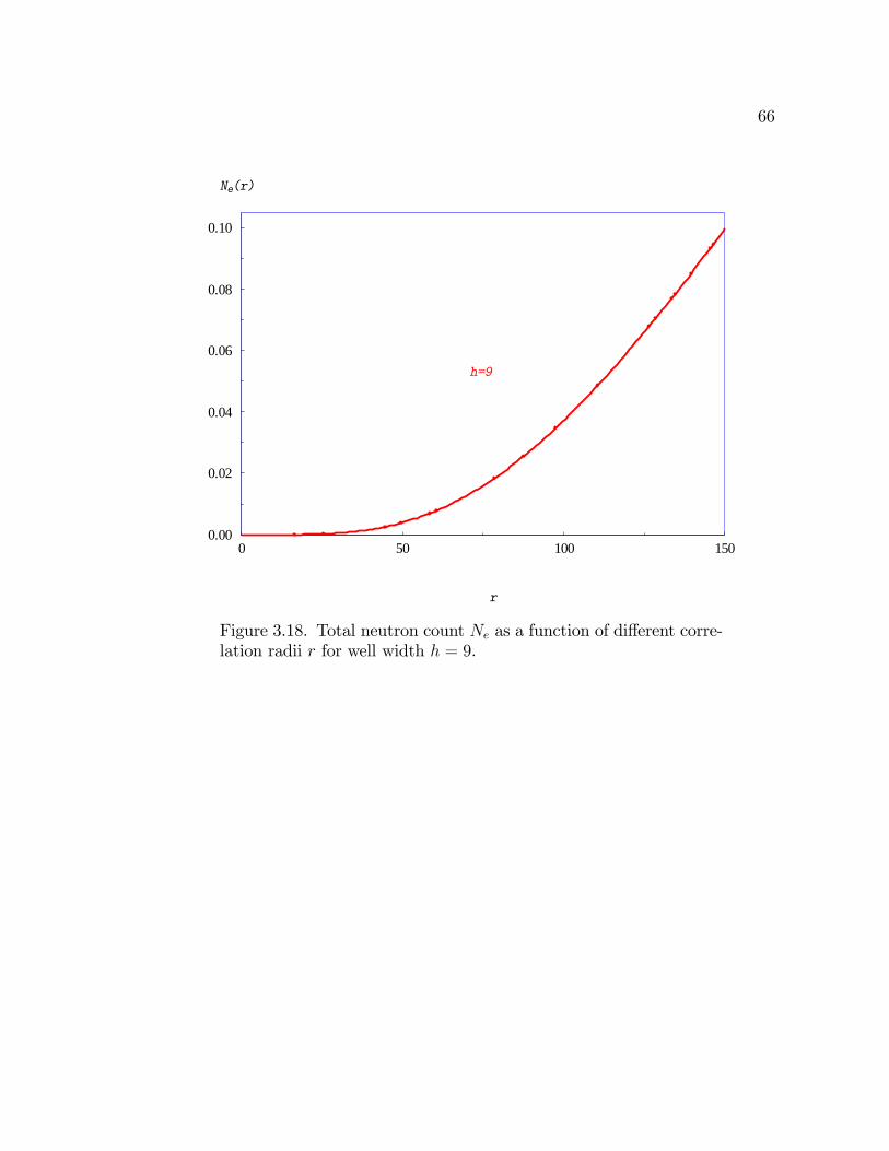
66

0 50 100 1500.00

0.02

0.04

0.06

0.08

0.10

r

Ne(r)

h=9

Figure 3.18. Total neutron count Ne as a function of di¤erent corre-lation radii r for well width h = 9.

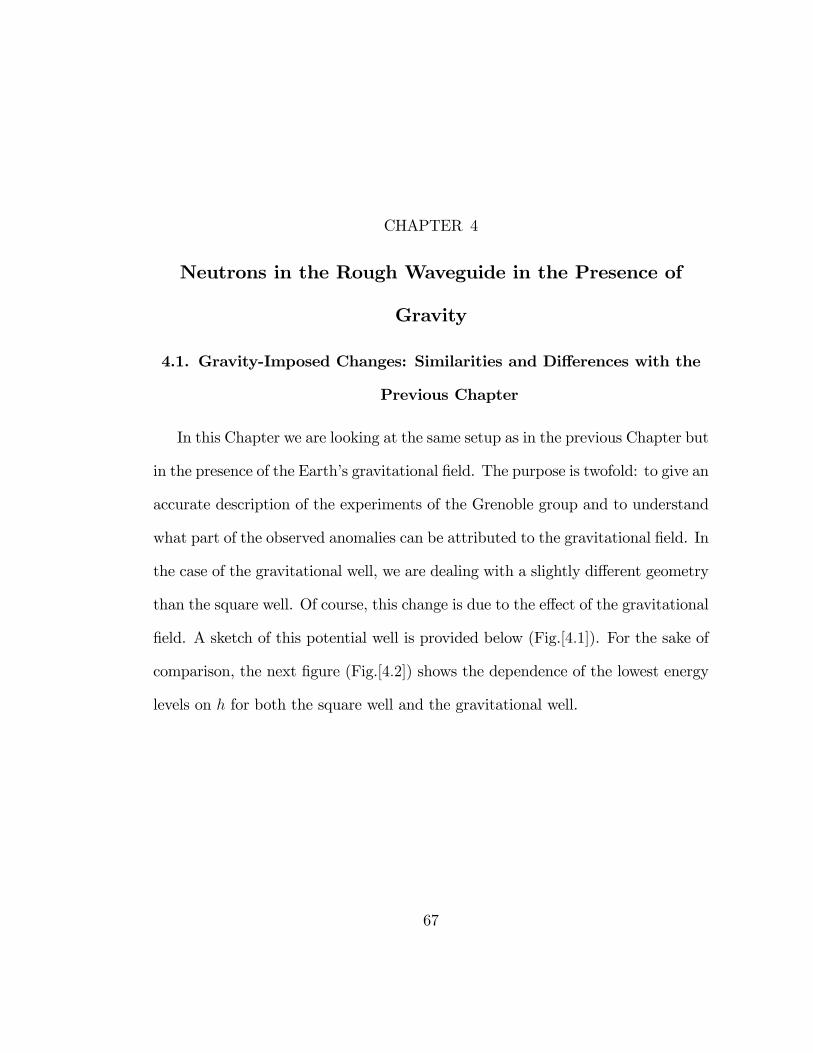
CHAPTER 4

Neutrons in the Rough Waveguide in the Presence of

Gravity

4.1. Gravity-Imposed Changes: Similarities and Di¤erences with the

Previous Chapter

In this Chapter we are looking at the same setup as in the previous Chapter but

in the presence of the Earth�s gravitational �eld. The purpose is twofold: to give an

accurate description of the experiments of the Grenoble group and to understand

what part of the observed anomalies can be attributed to the gravitational �eld. In

the case of the gravitational well, we are dealing with a slightly di¤erent geometry

than the square well. Of course, this change is due to the e¤ect of the gravitational

�eld. A sketch of this potential well is provided below (Fig.[4:1]). For the sake of

comparison, the next �gure (Fig.[4:2]) shows the dependence of the lowest energy

levels on h for both the square well and the gravitational well.

67

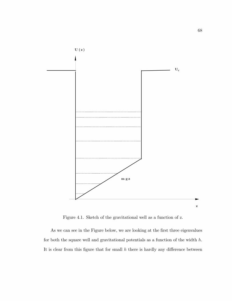
68

U (z )

z

m g z

Uc

Figure 4.1. Sketch of the gravitational well as a function of z.

As we can see in the Figure below, we are looking at the �rst three eigenvalues

for both the square well and gravitational potentials as a function of the width h.

It is clear from this �gure that for small h there is hardly any di¤erence between

69

2 3 4 5 6 7 8 9 100

2

4

6

8

10

λj(h)

h

λ1

λ2

λ3

Figure 4.2. The �rst three eigenvalues for both the square well andthe gravitational well as a function of the well width h. For bettercomparison, the bottom of the square well is chosen in the middle ofthe bottom of the gravitational well, mgh=2, and is drifting with h.The eigenvalues for the gravitational well are the lower curves, forthe SW-the upper.

the lowest eigenvalues of these two potentials; for larger h the di¤erences become

signi�cant.

Formally the transport equations for the rough waveguides with and without

gravity are the same as Eq.(1:14). However, the transition probabilities are dif-

ferent. This di¤erence, though signi�cant, is related mostly to the values of the

wavefunctions on the walls, i.e., to the coe¢ cients bj (h), Eq.(4:2).

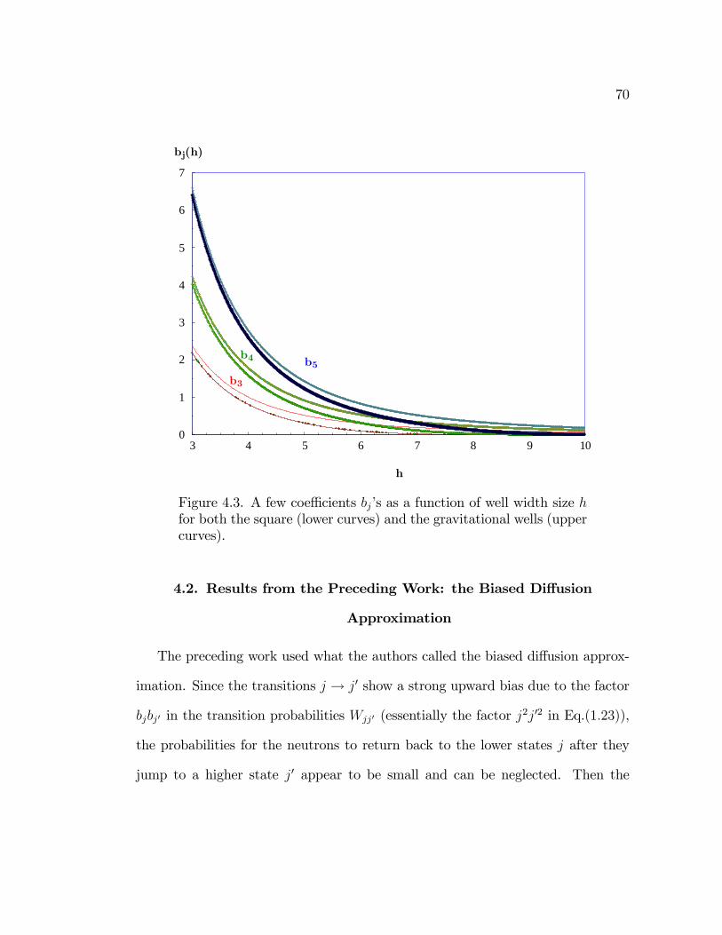
70

3 4 5 6 7 8 9 100

1

2

3

4

5

6

7

bj(h)

h

b5b4

b3

Figure 4.3. A few coe¢ cients bj�s as a function of well width size hfor both the square (lower curves) and the gravitational wells (uppercurves).

4.2. Results from the Preceding Work: the Biased Di¤usion

Approximation

The preceding work used what the authors called the biased di¤usion approx-

imation. Since the transitions j ! j0 show a strong upward bias due to the factor

bjbj0 in the transition probabilities Wjj0 (essentially the factor j2j02 in Eq.(1:23)),

the probabilities for the neutrons to return back to the lower states j after they

jump to a higher state j0 appear to be small and can be neglected. Then the

71

0 2 4 6 8 100

500

1000

1500

2000

2500

3000

λj(h)

h

Figure 4.4. The �rst nine coe¢ cients bj as a function of the widthof the channel h for the gravitational well. The lowest curve is b1and the highest b9.

absorption times � j are

(4.1)1

� j= m

Xj>j0

Zd�

2�Wjj0 (jqj � qj0j) ;

where � is the angle between qj and qj0. Note, that since the absorption threshold

uc is very high (� 105), direct transitions from the lower levels over the threshold

are negligible.

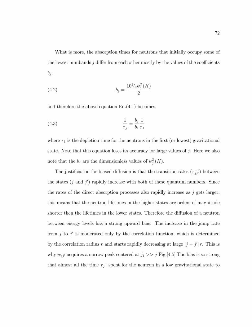
72

What is more, the absorption times for neutrons that initially occupy some of

the lowest minibands j di¤er from each other mostly by the values of the coe¢ cients

bj,

(4.2) bj =105l0

2j (H)

2

and therefore the above equation Eq.(4:1) becomes,

(4.3)1

� j=bjb1

1

� 1

where � 1 is the depletion time for the neutrons in the �rst (or lowest) gravitational

state. Note that this equation loses its accuracy for large values of j. Here we also

note that the bj are the dimensionless values of 2j (H).

The justi�cation for biased di¤usion is that the transition rates (��1jj0) between

the states (j and j0) rapidly increase with both of these quantum numbers. Since

the rates of the direct absorption processes also rapidly increase as j gets larger,

this means that the neutron lifetimes in the higher states are orders of magnitude

shorter then the lifetimes in the lower states. Therefore the di¤usion of a neutron

between energy levels has a strong upward bias. The increase in the jump rate

from j to j0 is moderated only by the correlation function, which is determined

by the correlation radius r and starts rapidly decreasing at large jj � j0j r. This is

why wjj0 acquires a narrow peak centered at j1 >> j Fig.[4:5] The bias is so strong

that almost all the time � j spent for the neutron in a low gravitational state to

73

transition up to higher states and over the absorption barrier is spent in the �rst

transition upwards.

The values of � j determine the depletion time of each quantum state. The

overall exit neutron count is

(4.4) Ne =X

Nj =X

Nj (0) exp (�L=vj� j) ;

where Nj (0) is the number of neutrons in a state j entering the waveguide of

length L. Additionally, for the lowest levels the velocities vj are almost the same,

vj �p"v0. The equation above can be rewritten using vj �

p"v0 and we can

directly get all the � j. Then it is easy for us to get the total neutron count which

is just a sum over all j. In the end, in the biased di¤usion approximation all the

pertinent parameters of roughness and the waveguide entering the exit neutron

count collapse into a single variable � Ref[8] and we get an analytical solution,

(4.5)Ne (h)

N0=Xj

exp (��bj (h))

where � is a complicated weighted integral of the correlation function that is

dependent on the correlation radius. If the roughness is two-dimensional,

(4.6) � = A2�2r2Z 1

0

z2 2 (y1; y (z)) dz

74

and

(4.7) A2 =

�2

�

�3=2� 10�5 tL

� 0uc�

3=2;

where 2 (y1; y) is the dimensionless zeroth harmonic of the correlation function

� (jqj � qj0j) over the angle between the vectors qj and qj0, and y1 = rp", y (z) =

y1p1� z2.

We can write the relaxation time � 1 for the lowest gravitational state as

(4.8)1

� 1= m

XZd�

2�W1j0

���q1�qj0��� ;where � is the angle between the vectors q1 and qj0. Finally, after replacing the

summation by the integration.

(4.9)� 0� 1= 2� 10�5u2c

��r

�2b1 (h)F2 (r; h) :

where

(4.10) F2 (r; h) ' r4r2uc��3

Z 1

0

dz z2 2 (y1; y) :

When we combine the equations Eq.(4:9) and Eq.(4:10) we get the following equa-

tion,

(4.11) � (�; r) = A2�2r2Z 1

0

dz z2 2 (y1; y)

75

This concludes the description of the preceding work, which provides the approx-

imate analytical expression to the exit neutron count. We will now describe how

we deal with the same problem computationally without relying on the biased

di¤usion approximation.

4.3. Exact Calculation of the Absorption Time

In our case we are not using the biased di¤usion approximation, but actually

using the brute force technique to solve the full set of transport equations numer-

ically.

As a result, we do not get a nice analytical solution to the problem. Instead we

use the full matrix, meaning the matrix with transitions upwards and downwards,

for which we can only get a numerical solution. The structure of the diagonal and

o¤-diagonal elements in the matrix transport equations is di¤erent. The diagonal

elements have the structure de�ned below in Eq.(4:12), where for an element in

row j we are summing over all the elements j0. The o¤-diagonal elements are

simpler: these are simply wjj0. We rewrite the transition probabilitiesWjj0 de�ned

in Eq.(1:22) that represent the diagonal elements of the matrix, in a notation that

is closer to the one that was used in the most recent papers in this �eld. Therefore

speci�cally for diagonal elements of our matrices, when j = j0, we write,

(4.12) Fj (r; h) =

r2

�� 10�5r4bj

Xj0 6=j

bj0 2 (y1; yj0) ;

76

where 2 (y1; yj0) here also represents the dimensionless zeroth harmonic of the

correlation function over the angles between the vectors qj and qj0. Since we

are not working under the context of biased di¤usion, we can only perform our

computations numerically.

We have o¤-diagonal elements in our matrix for square well are de�ned in

dimensionless units as

(4.13) wjj0 =32r2�2p2�h2

��j

h

�2��j0

h

�2E ()�

1 + r2 (q � q0)2q1 + r2 (q + q0)2

� ;where

(4.14) = 2r

sqq0�

1 + r2 (q + q0)2� :

Hence our total matrix, which we will call Mjj0 looks like

(4.15) Mjj0 =

0BBBBBBBBBBB@

F11 w12 :: : w1smax

w21 : : : w2smax

: : : : :

: : : : :

w2smax : : : Fsmax;smax

1CCCCCCCCCCCA:

More detailed mathematics regarding the Fjj0 = Fj (r; h) for the discrete case

will be available in Appendix C.

77

We do not have a simple analytical description of the gravitational states sim-

ilar to that for the square well states in the previous chapter. However, for the

states with high index j, and especially at small h, the di¤erence between the

gravitational and square well states is negligible. Therefore, for higher states we

can replace the gravitational states by the square well states.

As a result, our square matrix of transition probabilities acquires a block struc-

ture. One block representing the transitions between gravitational states, two of

the blocks represent the transitions between the lower gravitational states and

higher square well states, and the third block represents the transitions between

higher square well states. Once we have the total matrix with all the block compo-

nents, we are numerically computing the eigenvalues and eigenvectors of the total

matrix. We can write the neutron exit count in terms of these absorption times � j

in quite a simple form,

(4.16)Ne (h)

N0=Xj

exp

�� tL� j (h)

�;

where tL is the time of �ight of the UCNs between the mirrors. Note that the

above equation was introduced in the previous section and chapter as it is a general

equation that can be used with and without the biased di¤usion approximation.

It is interesting to note that the center of the peak of the transition probabilities

Wjj0 for transitions from j to j0 is located at some j1 >> j, see Fig.[4:5] for example.

78

0 100 200 300 400 500 600 7000

50

100

150

200

250

300

j'

W1j'

h = 7

Figure 4.5. The transition probabilities W1j0 as a function ofj0exhibit the peak around j0 = 100.

The peak is very high and relatively narrow.

4.4. Numerical Results

In this section we present the main results of the thesis as pertaining to the

Grenoble experiments. As in the previous section regarding the square well poten-

tial, we are now looking at the exit neutron count in the gravitational potential.

The gravitational potential was introduced in a previous chapter. However, we will

reproduce a schematic �gure here. In this �gure, the particles on the lowest three

levels "classically" do not reach the rough ceiling, do not scatter, and survive for a

79

long time. The particles from the higher levels are actively scattered on the rough

ceiling, go rapidly upwards, and get absorbed by the walls. When the width of

the waveguide h becomes smaller, all the levels are rapidly squeezed up (see Fig.

below).

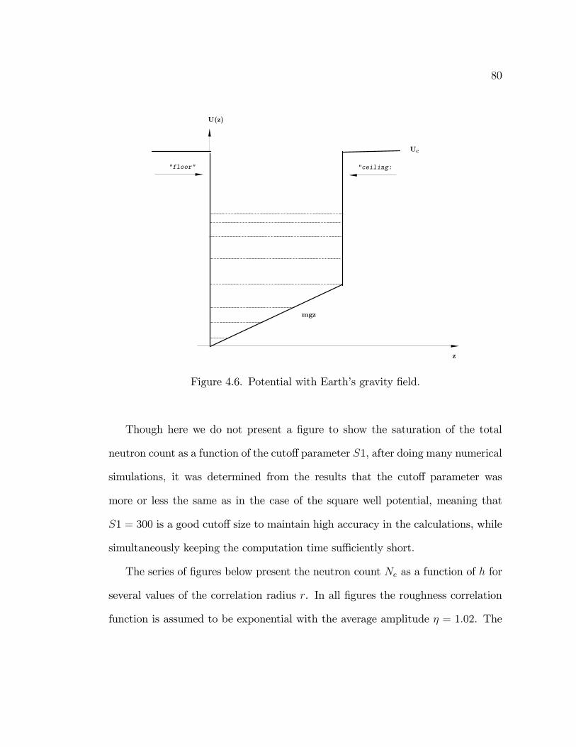
80

U(z)

z

mgz

Uc

"floor" "ceiling:

Figure 4.6. Potential with Earth�s gravity �eld.

Though here we do not present a �gure to show the saturation of the total

neutron count as a function of the cuto¤parameter S1, after doing many numerical

simulations, it was determined from the results that the cuto¤ parameter was

more or less the same as in the case of the square well potential, meaning that

S1 = 300 is a good cuto¤ size to maintain high accuracy in the calculations, while

simultaneously keeping the computation time su¢ ciently short.

The series of �gures below present the neutron count Ne as a function of h for

several values of the correlation radius r. In all �gures the roughness correlation

function is assumed to be exponential with the average amplitude � = 1:02. The

81

current rough mirror used by the Grenoble group probably has r = 0:65 and

� = 1:02. As one can see, all the �gures are similar, though the curves slowly shift

to the left with increasing r. This is understandable: the surface becomes �atter

with increasing r and the neutrons survive longer.

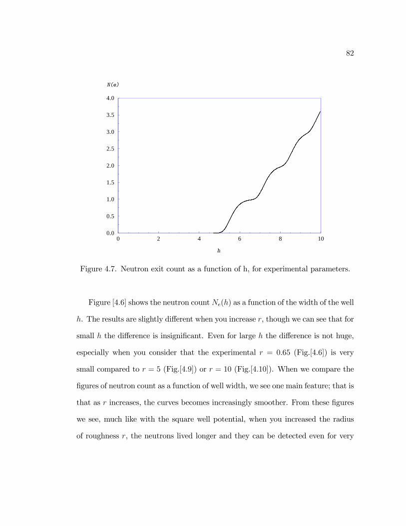
82

0 2 4 6 8 100.0

0.5

1.0

1.5

2.0

2.5

3.0

3.5

4.0

h

N(e)

Figure 4.7. Neutron exit count as a function of h, for experimental parameters.

Figure [4:6] shows the neutron countNe(h) as a function of the width of the well

h. The results are slightly di¤erent when you increase r, though we can see that for

small h the di¤erence is insigni�cant. Even for large h the di¤erence is not huge,

especially when you consider that the experimental r = 0:65 (Fig.[4:6]) is very

small compared to r = 5 (Fig.[4:9]) or r = 10 (Fig.[4:10]). When we compare the

�gures of neutron count as a function of well width, we see one main feature; that is

that as r increases, the curves becomes increasingly smoother. From these �gures

we see, much like with the square well potential, when you increased the radius

of roughness r, the neutrons lived longer and they can be detected even for very

83

0 2 4 6 8 100.0

0.5

1.0

1.5

2.0

2.5

3.0

3.5

h

N(e)

r = 0.1

Figure 4.8. Neutron count as a function of h for correlation radiusradius of roughness r = 0:1.

small width h. This is happening as well in the case of the gravitational potential.

We see that as the radius of roughness gets larger and larger, the neutrons survive

for smaller and smaller well width sizes.

For very large r, for example in the �gures where r = 500 (Fig.[4:15]) and

r = 1000 (Fig.[4:16]), we see that the curve �attens and we don�t have the well

de�ned steps that we see at smaller values of r, implying that the discrete energy

levels cannot be detected so easily as with smaller r. However, it should be noted

that this �attening happens only for unrealistically large r. In general the steps

on the curves are very robust and the �rst bump remains detectable even for very

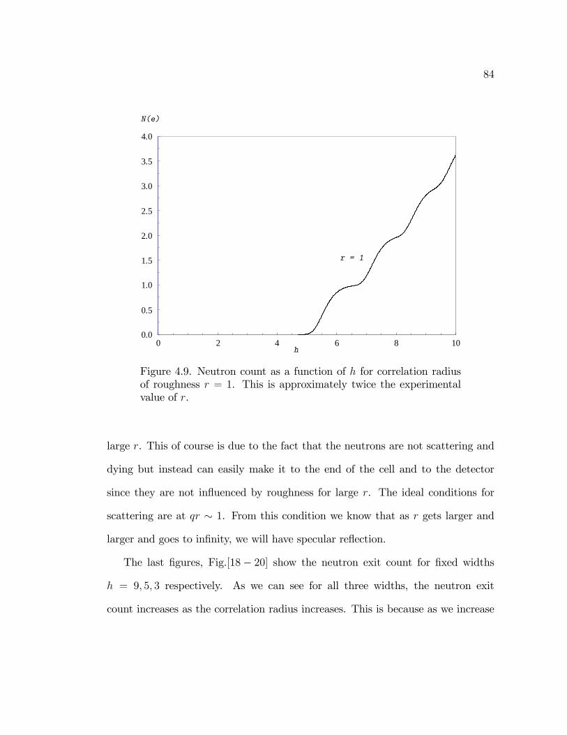
84

0 2 4 6 8 100.0

0.5

1.0

1.5

2.0

2.5

3.0

3.5

4.0

r = 1

h

N(e)

Figure 4.9. Neutron count as a function of h for correlation radiusof roughness r = 1. This is approximately twice the experimentalvalue of r.

large r. This of course is due to the fact that the neutrons are not scattering and

dying but instead can easily make it to the end of the cell and to the detector

since they are not in�uenced by roughness for large r. The ideal conditions for

scattering are at qr � 1. From this condition we know that as r gets larger and

larger and goes to in�nity, we will have specular re�ection.

The last �gures, Fig.[18� 20] show the neutron exit count for �xed widths

h = 9; 5; 3 respectively. As we can see for all three widths, the neutron exit

count increases as the correlation radius increases. This is because as we increase

85

0 2 4 6 8 100.0

0.5

1.0

1.5

2.0

2.5

3.0

3.5

4.0

r = 5

h

N(e)

Figure 4.10. Neutron count as a function of h for correlation radiusof roughness r = 5.

the correlation radius, the ceiling becomes smoother, and therefore there is less

scattering and absorbtion by the rough wall.

4.5. Conclusions

It is interesting to compare these results with the previous results without

gravity in the square well section.

� The dependence of the exit neutron count on r was much more signi�cant

in the case of the square well potential: Ne (r) at �xed h changed by many

orders of magnitude.

86

0 2 4 6 8 100.0

0.5

1.0

1.5

2.0

2.5

3.0

3.5

4.0

N(e)

h

r = 10

Figure 4.11. Neutron count as a function of h for correlation radiusof roughness r = 10.

� It is interesting to note that the ratio of the relaxation times for the

diagonal case (in which we do not take into account the transitions between

the states, meaning the cases where j 6= j0) and the case described in this

section (where we allow all the transitions, and not just the biased ones, to

be taken into account) � diag=� full is close to 1. This was rather unexpected.

� It is also interesting to note that the ratio of the results for the matrix in

the square well potential and the matrix in the gravity potential goes to

one as h goes to 0, � jSqwell=� jgrav ! 1 as h ! 0 since all the levels are

87

0 2 4 6 8 100.0

0.5

1.0

1.5

2.0

2.5

3.0

3.5

4.0

r = 20

h

N(e)

Figure 4.12. Neutron count as a function of h for correlation radiusof roughness r = 20.

being squeezed up and the di¤erence in potentials near the bottom of the

well looses its signi�cance.

� The major result of this section is the exit neutron count in the presence

of gravity. It illustrates the total neutron count Ne(h) as a function of

the width of the channel h. When comparing this result to the work done

previously using the biased di¤usion approximation, we see that the curves

are similar. This means that the biased di¤usion approximation is indeed

a very robust approximation.

88

0 2 4 6 8 100.0

0.5

1.0

1.5

2.0

2.5

3.0

3.5

4.0

N(e)

h

r=30

Figure 4.13. Neutron count as a function of h for correlation radiusof roughness r = 30.

� In almost all computations the exit neutron count as a function of cell

width Ne (h) retained the step-wise nature. This may be considered as a

unequivocal proof of quantization of neutron motion by the Earth gravi-

tational �eld.

89

0 2 4 6 8 100

1

2

3

4

5

N(e)

h

r = 50

Figure 4.14. Neutron count as a function of h for correlation radiusof roughness r = 50.

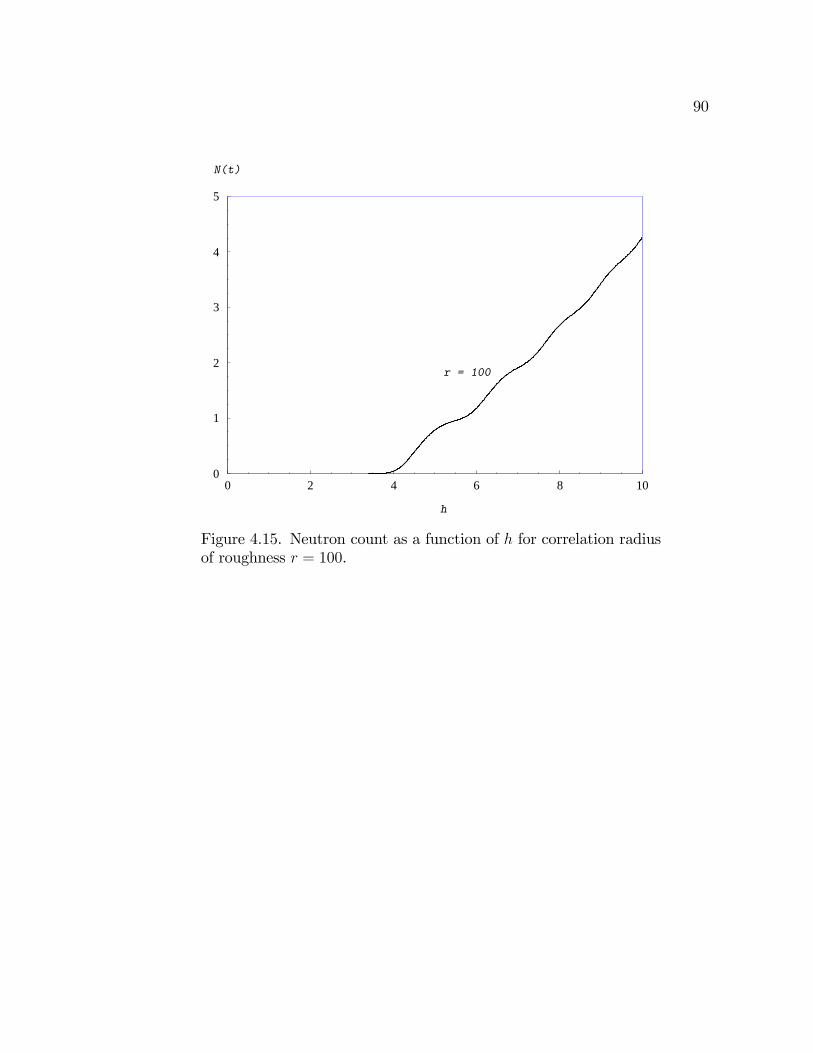
90

0 2 4 6 8 100

1

2

3

4

5

r = 100

h

N(t)

Figure 4.15. Neutron count as a function of h for correlation radiusof roughness r = 100.

91

0 2 4 6 8 100

1

2

3

4

5N(e)

h

r = 500

Figure 4.16. Neutron count as a function of h for correlation radiusof roughness r = 500.

92

0 2 4 6 8 100

1

2

3

4

5

6

r = 1000

h

N(e)

Figure 4.17. Neutron count as a function of h for correlation radiusof roughness r = 1000.

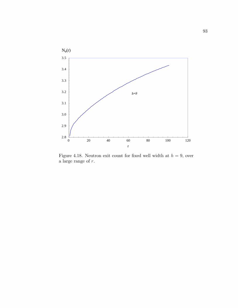
93

r0 20 40 60 80 100 120

2.8

2.9

3.0

3.1

3.2

3.3

3.4

3.5

Ne(r)

h=9

Figure 4.18. Neutron exit count for �xed well width at h = 9, overa large range of r.

94

r0 20 40 60 80 100 120

0.0

0.1

0.2

0.3

0.4

0.5

0.6

0.7

0.8

h=5

Ne(r)

Figure 4.19. Neutron exit count for �xed well width at h = 5, overa large range of r.

95

r

0 50 100 150 2000.0

0.2

0.4

0.6

0.8

1.0

Ne(r)

h=3

Figure 4.20. Neutron exit count for �xed well width at h = 3, overa large range of r.

CHAPTER 5

Summary and Conclusions

5.1. Main Conclusions

In summary, the main goal of this thesis was to provide a rigorous theoretical

description for the di¤usion of ultra cold neutrons (UCN) through narrow rough

channels. We used the general transport theory of particles along rough surfaces to

the gravitationally quantized di¤usion of UCN in a rough waveguide. We looked at

two separate problems: di¤usion of the neutrons through rough waveguides on the

way from the reactor to the experimental cell and the neutron count for neutrons

exiting experimental cell with absorbing walls in the square well potential as well

as the gravitational potential. We used numerical calculations to investigate the

e¤ect of two types of random roughness on the di¤usion coe¢ cient, as well as

to evaluate the neutron count using the experimental input parameters in both

potentials.

The main content of Chapter 2 is the calculations of the di¤usion coe¢ cient

and the mean free path for ultra-cold neutrons in narrow channels with random

rough walls. We determined that if one wants to e¤ectively turn back the neutrons

which got into the gaps in the channel junctions, one should make the correlation

radius of surface roughness as small as possible. We compared the behavior of d (r)

96

97

and l(r) for surfaces with the Gaussian and the exponential correlation functions

of surface roughness. We found that there is a complicated minimum in d (r)

and l(r) for small correlation radius r � 2 � 10�4. Additionally we found that

the di¤usion coe¢ cient and the MFP rapidly increase as the correlation radius r

increases, though at di¤erent rates depending on the surface correlation function.

The growth of the di¤usion coe¢ cient and MFP is not monotonic, there is more

then one minimum at qj � 1=r. We saw that at large r the function d (r) behaves

roughly as r3, where the exponent slightly drifts with r. The computations were

done for realistic values of the channel width h = 8:52. At di¤erent values of h the

results were qualitatively the same. The growth of d (r) and l(r) for the Gaussian

surface correlation function is much faster than for the exponential correlation

function. As a result, it is preferable to have the junction walls with exponential

correlation of inhomogeneities.

The conclusions for Chapter 3 regarding the UCN in the square well potential

are as follows: Irrespective of the well width and the correlation radius, a good

cuto¤ parameter for all computations is around S1 = 300. We see that as the

radius of roughness r increases, the total neutron count goes to zero for smaller

and smaller values of h. However, as we can see from the plots, the numbers

that we get for Ne(h) are always extremely small, so essentially all the neutrons

die almost immediately. As we will see in this Chapter, this is not the case for

the gravitational well. Hence, we can say that the square well approximation is

very poor for this particular problem: though the weak Earth gravitational �eld

98

introduces only a small distortion near the bottom of the potential well, its e¤ect

on the neutron survival rate is very large.

The main conclusion for Chapter 4 is the exit neutron count in the presence

of gravity. It illustrates the total neutron count Ne(h) as a function of the width

of the channel h. When comparing this result to the work done previously using

the biased di¤usion approximation, we see that the curves are similar. This means

that the biased di¤usion approximation is a very robust approximation. This result

was a somewhat surprising result. Other conclusions include the following. The

dependence of the exit neutron count on r was much more signi�cant in the case

of the square well potential where Ne (r) at �xed h changed by many orders of

magnitude. It is interesting to note that the ratio of the relaxation times for the

diagonal case (in which we do not take into account the transitions between the

states, meaning the cases where j 6= j0) and the case described in this Chapter

(where we allow all the transitions, and not just the biased ones to be taken

into account) � diag=� full is close to 1. This was rather unexpected. It is also

interesting to note that the ratio of the results for the square well potential and

the gravitational potential goes to one as h goes to 0, � jSqwell=� jgrav ! 1 as h! 0

since all the levels are being squeezed up and the di¤erence in potentials near the

bottom of the well loses its signi�cance, see Figure above.

99

5.2. Recommendations for Future Work

Using rough mirrors as a quantum state selector can be extended beyond this

series of GRANIT experiments. Some of the more exciting experiments include

the observation of quantum gravitational states for other ultra-cold particles and

anti-particles in the context of the GBAR experiment at CERN.

One of the main goals of the GBAR experiments is to measure the acceleration

in free fall of ultra-cold neutral anti hydrogren atoms in the Earth�s gravitational

�eld. The experiment entails using anti hydrogen ions, which consist of one an-

tiproton supplied by the ELENA deceleration ring at CERN and two positrons

created by the linac, and cooling them below 10 �K with Beryllium plus ions.

Their positive charge makes them easier to manipulate. Using lasers, their veloc-

ity can be reduced to half a meter per second. Once they are trapped by an electric

�eld, one of their positrons will be removed with laser, which will make it neutral.

Hence, at this point the Earth�s gravitational �eld will be the only force acting

upon them, and they will be able to free fall a given distance, and their time of fall

could be measured. The results of this experiment are much anticipated, because

it could potentially mean that gravity might have a di¤erent e¤ect on antimatter

then it does on matter.

For the past 60 years, there has also been an ongoing search for the neutron

electric dipole moment (nEDM). Over the course of the decades the accuracy of

(negative) results has been improved by many orders of magnitude. The nEDM

100

potentially violates CP symmetry, meaning that it violates the presumption that

if a particle and a respective anti particle are interchanged, while their spatial

coordinates are inverted, then the laws of physics should remain the same. The

goal of these ongoing and future nEDM experiments is to improve the sensitivity

for detection nEDM by orders of magnitude. One of the experiments being done

at Oak Ridge National Laboratory is to create a three-component �uid described

as isotopically puri�ed Helium-4, a trace amount of spin-polarized Helium-3, and

spinpolarized ultra-cold neutrons. Then once that �uid has been created, it should

be exposed to a small but homogeneous magnetic �eld and a large electric �eld.

The nEDM could then be measured by looking at the neutron precession frequency

which is linearly dependent on the magnitude of the electric �eld strength, and

whose sign is dependent on the alignment between the magnetic and electric �elds.

Above are just examples of the experiments that are ongoing or planned for the

near future, however, our theoretical work on the use of rough mirrors as quantum

state selectors are well suited for dealing with these and similar applications.

APPENDIX A

Dimensionless Transition Probabilities

In this Appendix we make the equations for the harmonics of the transition

probabilities dimensionless. According to Ref.[[2]], the angular harmonics of the

transition probabilities for surfaces with Gaussian correlations of surface inhomo-

geneities. are

(A.1)

W(0;1)jj0 =

}m2H2

��j

H

�2��j0

H

�24�l2R2I0(QQ

0)Exp(�QQ0)Exp(�12(Q�Q0)2):

Then

(A.2)

W(0;1)jj0 �w0 =

}m2H2

��j

h

�2��j0

h

�24��2r2I0(QQ

0)Exp(�QQ0)Exp(�12(Q�Q0)2)

where w0 = m� 0, with � 0 = (4ml20)=(p2�}). As a result the dimensionless equa-

tions become

(A.3)

w(0;1)jj0 =

}m2H2

��j

h

�2��j0

h

�24��2r2

�m4ml20p2�}

�I0(QQ

0)Exp(�QQ0)Exp(�12(Q�Q0)2)

101

102

(A.4)

w(0;1)jj0 =

4l20p2�H2

(4��2r2)

��j

h

�2��j0

h

�2I0(QQ

0)Exp(�QQ0)Exp(�12(Q�Q0)2)

(A.5) w(0;1)jj0 =

8��2r2p2�h2

��j

h

�2��j0

h

�2I0(QQ

0)Exp(�QQ0)Exp(�12(Q�Q0)2)

Therefore, our �nal equation for the transition probability for the Gaussian

correlator becomes

(A.6)

w(0;1)jj0 =

8�p2�

� rh

�2��jh

�2��j0

h

�2I(0,1)(QQ

0)Exp(�QQ0)Exp(�12(Q�Q0)2)

Note that in computations we assume the scaling parameter � = 1.

Additionally, in the same way, we derive the dimensionless transition probabil-

ities for the exponential roughness,

(A.7) w(0)jj0 =

32r2p2�h2

��j

h

2�2�

�j0

h

�2 E(2rq

qjqj0

(1+r2(qj+qj0 )2))

(1 + r2(qj � qj0)2)(p1 + r2(qj + qj0)2)

(A.8)

w(1)jj0 =

16p2�h2

��j

h

�2��j0

h

�2�(1 + r2(q2j + q2j0))E(2r

qqjqj0

(1+r2(qj+qj0 )2))� (1 + r2(qj � qj0)

2)K(2rq

qjqj0

(1+r2(qj+qj0 )2))

(1 + r2(qj � qj0)2)(p1 + r2(qj + qj0)2)

;

APPENDIX B

Asymptotic Expansion for Transition Probabilities for

Surfaces with Exponential Roughness Correlator

Here we present an asymptotic expansion for the transition probabilities for

the surfaces with the exponential roughness correlator.

We need an asymptotic expression for:

(B.1) Exp(�x2) � (I0(x2)� I1(x2))

At large x,

(B.2) I0(x2) s

Exp(�x2)p2�x2

�1�

��18x2

�+

�(�1)(�9)2!(8x)2

�� :::

�

since

(B.3) I0(x2) s

Exp(�x2)p2�x2

�1 +

�1

8x2

��

and,

(B.4) I1(x2) s

Exp(�x2)p2�x2

�1�

�4� 18x2

�+

�(4� 1)(4� 9)4 � 64 � x4

�� :::

�

103

104

(B.5) I1(x2) s

Exp(�x2)p2�x2

�1�

�3

8x2

��

As a result,

(B.6)

w(0;1)jj0 =

8�p2�

� rh

�2��jh

�2��j0

h

�2I(0;1)(QQ

0)Exp(�QQ0)Exp(�12(Q�Q0)2)

If we replace the exact transition probabilities by these asymptotic expansions,

we get almost identical numerical results. We tried using this expansion to see if

we could speed up computation time

APPENDIX C

Diagonal Elements of Transition Probabilities for the

Biased Di¤usion Approximation

In this Appendix we try to replace the summation over discrete states in

Eq.(4:12) by integration. Starting from the equation, Eq.(4:12) and using the

following de�nitions,

bj = 105�jh uc

;(C.1)

�j =�2j2

h2;(C.2)

F2 (r; h) =

r2

�� 10�5r4

Xj0>1

bj0 2 (y1; yj0)

we can rewrite this expression in the following way

F2 (r; h) =

r2

�� 10�5r4

Xj0>1

105�jh uc

2 (y1; yj0)(C.3)

=

r2

�r4Xj0>1

�jh uc

2 (y1; yj0)(C.4)

=

r2

�r4�

�2

h3uc

�Xj0>1

j02 2 (y1; yj0)(C.5)

105

106

Now note that N =h�"12 , and � = uc

", therefore we know that N =h

�

�uc�

� 32. It

should also be noted that we can write�

�2

h3uc

�as follow,

��2

h3uc

�=

���3=2

u1=2c

��1���3=2

u1=2c

���2

h3uc

�(C.6)

=u1=2c

��3=2

!��3�3=2

h3u3=2c

�(C.7)

=u1=2c

��3=2

!�1

N

�(C.8)

hence we can rewrite F2 (r; h) as,

(C.9) F2 (r; h) =

r2

�r4

u1=2c

��3=2

!1

N 3

Xj0>1

j02 2 (y1; yj0)

Now to make this a continuous function we can replace the sum by an integral,

(C.10) F2 (r; h) =

r2

�r4

u1=2c

��3=2

!1

N 3

Z N

1

j02 2 (y1; yj0)

where we substitute z = jN and dj

N = dz and then we can write z2 = j2

N 2 . The

above equation now becomes,

F2 (r; h) =

r2

�r4

u1=2c

��3=2

!1

N 3

Z 1

0

z2N 2 dzN 2 (y1; yj0)(C.11)

=

r2

�r4

u1=2c

��3=2

!Z 1

0

dz z2 2 (y1; yj0) ;(C.12)

which is Eq.(4:10) in the main text. This equation was used in Ref??.

Bibliography

[1] A. Meyerovich and V. V. Nesvizhevsky, "Gravitational quantum states ofneutrons in a rough waveguide," Phys. Rev. A, vol. 73, 063616, June 2006.

[2] R. Adhikari, Y. Cheng, and A. E. Meyerovich, "Quantum size e¤ect andbiased di¤usion of gravitationally bound neutrons in a rough waveguide,"Phys. Rev.A, vol. 75, 063613, June 2007.

[3] A. E. Meyerovich and A. Stepaniants, "Quantized systems with randomlycorrugated walls and interfaces," Phys. Rev. B, vol. 60, no. 12, p. 9129, 1999.

[4] A. E. Meyerovich and A. Stepaniants, "Transport equation and di¤usion inultrathin channels and �lms," Phys. Rev. B, vol. 58, p. 13 242, Nov. 1998.

[5] A. E. Meyerovich and A. Stepaniants, "Transport phenomena at rough bound-aries," Phys. Rev. Lett., vol. 73, no. 2, p. 316, July 1994.

[6] Y. Cheng and A. E. Meyerovich, "Mode coupling in quantized high-quality�lms," Phys. Rev. B, vol. 73, 085404, Feb. 2006.

[7] A. E. Meyerovich and I. V. Ponomarev, "Surface roughness and size e ects inquantized �lms," Phys. Rev. B, vol. 65, 155413, 2002.19

[8] M. Escobar and A. Meyerovich, "Beams of gravitationally bound ultra-coldneutrons in a rough waveguide," Phys. Rev. A, vol. 83, 033618, Mar. 2011.

[9] M. Escobar and A. Meyerovich, "Applications and identi�cation of surfacecorrelations," arXiv:1404.1291, 2014.

[10] M. Escobar and A. Meyerovich, "Quantized ultra-cold neutrons in roughwaveguides: GRANIT experiments and beyond," Advances in High EnergyPhysics, vol. 2014, Article ID: 185414, July 2014.

107

108

[11] M. Escobar, F. Lamy, A. E. Meyerovich, and V. V. Nesvizhevsky, "Roughmirror as a quantum state selector: analysis and design," Advances in HighEnergy Physics, vol. 2014, Article ID: 764182, Aug. 2014.

[12] M. Escobar and A. E. Meyerovich, "Quantum transport equation for systemswith rough surfaces and its application to ultra-cold neutrons in a quantizinggravity �eld," Journal of Experimental and Theoretical Physics, vol. 119, no.6, pp. 1123{1133, 2014.

[13] M. Escobar, "Quantum Di¤usion Of Ultra-Cold Neutrons in a RoughWaveguide in a Gravity Field", University of Rhode Island, 2015.

[14] V. V. Nesvizhevsky, H. G. Borner, A. K. Petukhov, H. Abele, S. Baessler, F.J. Rueb, T. Stoferle, A. Westphal, A. M. Gagarski, G. A. Petrov, and A. V.Strelkov, "Quantum states of neutrons in Earth�s gravitational �eld,"Nature,vol. 415, pp. 297{299, Nov. 2002.

[15] V. V. Nesvizhevsky, "Investigation of quantum neutron states in the terrestrialgravitational �eld above a mirror," Physics-Uspekhi, vol. 47 (5), p. 515, 2004.

[16] V. V. Nesvizhevsky, H. G. Borner, A. M. Gagarski, A. K. Petoukhov, G. A.Petrov, H. Abele, S. Baessler, G. Divkovic, F. J. Rueb, T. Stoferle, A. West-phal, A. V. Strelkov, K. V. Protasov, and A. Y. Voronin, "V. V. Nesvizhevsky,"Investigation of quantum neutron states in the terrestrial gravitational �eldabove a mirror," Phys. Rev. D, vol. 67, 102002, 2003.

[17] V. V. Nesvizhevsky, A. K. Petukhov, H. G. Borner, T. A. Baranova, A. M.Gagarski, G. A. Petrov, K. V. Protasov, A. Y. Voronin, S. Baessler, H. Abele,A. Westphal, and L. Lucovac, "Study of the neutron quantum states in thegravity �eld," Eur. Phys. J. C, vol. 40, pp. 479{491, 2005.

[18] V. V. Nesvizhevsky, H. Borner, A. M. Gagarski, G. A. Petrov, A. K. Petukhov,H. Abele, S. Baessler, T. Stoferle, and S. M. Soloviev, "Search for quantumstates of neutron in a gravitational �eld: gravitational levels," Nuclear Instru-ments and Methods in Physics Research A, vol. 440, pp. 754{759, 2000.

[19] V. V. Nesvizhevsky and K. V. Protasov, Trends in Quantum Gravity Re-search.Nova Science Publishers, Inc., 2006.20

109

[20] I. Antoniadis, S. Baessler, O. Bertolami, D. Dubbers, A. Meyerovich, V.V. Nesvizhevsky, K. Protasov, and S. Reynaud, C. R. Physique 12, vol. 8,pp.703{706, Oct. 2011.

[21] S. Baessler, M. Beau, M. Kreuz, V. N. Kurlov, V. V. Nesvizhevsky, G. Pignol,K. V. Protasov, F. Vezzu, and A. Y. Voronin, "The GRANIT spectrometer,"C. R. Physique, vol. 12, pp. 707{728, 2011.

[22] S. Baessler, A. M. Gagarski, E. V. Lychagin, A. Mietke, A. Y. Muzychka,V. V.Nesvizhevsky, G. Pignol, A. V. Strelkov, B. P. Toperverg, and K. Zher-nenkov, "New methodical developments for GRANIT," C. R. Physique, vol.12, pp.729{754, 2011.

[23] A. Westphal, "Quantum Mechanics and Gravitation," Ph.D. disserta-tion,University of Heidelberg, 2001. [Online]. Available: arxiv.org/pdf/gr-qc/0208062.

[24] C. Krantz, "Quantum States of Neutrons in the GravitationalField,"Ph.D. dissertation, University of Heidelberg, 2006. [Online].Available:http://www.physi.uni-heidelberg.de/Publications/

[25] A. Y. Voronin, H. Abele, S. Baessler, K. V. Protasov, and A. West-phal,"Quantum motion of a neutron in a wave-guide in the gravitational�eld,"Phys. Rev. D, vol. 73, 044029, Feb. 2006.

[26] V. V. Nesvizhevsky, K. Petukhov, K. V. Protasov, and A. Y. Voronin, "Cen-trifugal quantum states of neutrons," Phys. Rev. A, vol. 78, 033616, 2008.

[27] V. V. Nesvizhevsky and A. Y. Voronin, "Centrifugal quantum states of neu-trons," C. R. Physique, vol. 12, pp. 791{795, 2011.

[28] A. Y. Voronin, P. Froelich, and V. V. Nesvizhevsky, "Gravitational quantumstates of antihydrogen," Phys. Rev. A, vol. 83, 032903, Mar. 2011.

[29] A. Y. Voronin, V. V. Nesvizhevsky, and S. Reynaud, "Whispering-gallery ofantihydrogen near a curved surface," Phys. Rev. A, vol. 85, 014902.

[30] G. Dufour, P. Debu, A. Lambrecht, V. V. Nesvizhevsky, S. Reynaud, and A.Y. Voronin, "Shaping the distribution of vertical velocities of antihydrogen inGBAR," arXiv:1312.5534v1 [quant-ph], 2002.

110

[31] P. Crivelli, V. V. Nesvizhevsky, and A. Y. Voronin, "Can we ob-serve the gravitational quantum states of Positronium?" arXiv:1408.7051v1[physics.atomph], 2014.

[32] A. Y. Voronin, V. V. Nesvizhevsky, and S. Reynaud, "Whispering-gallerystates of antihydrogen near a curved surface," Nature Physics, vol. 6, 114-1172010.21

[33] I. Antoniadis, S. Baessler, M. Buchner, V. V. Fedorov, S. Hoedl, A. Lambrecht,V. V. Nesvizhevsky, G. Pignol, K. V. Protasov, S. Reynaud, and Y. Sobolev,"Short-range fundamental forces," C. R. Physique, vol. 12, pp. 775{778, 2011.

[34] S. Baessler, V. V. Nesvizhevsky, G. Pignol, K. V. Protasov, and A. Y. Voronin,"Constraints on spin-dependent short-range interactions using gravitationalquantum levels of ultra-cold neutrons," arXiv:0902.3139, 2009.

[35] M. Kreuz, V. V. Nesvizhevsky, P. Schmidt-Wellenburg, T. Soldner, M.Thomas, H. G. Borner, F. Naraghi, G. Pignol, K. V. Protasov, D. Rebreyend,F. Vezzu, R. Flaminio, C. Michel, N. Morgado, L. Pinard, S. Baessler, A. M.Gagarski, L. A. Grigorieva, T. M. Kuzmina, A. E. Meyerovich, L. P. Mezhov-Deglin, G. A. Petrov, A. V. Strelkov, and A. Y. Voronin, "A method tomeasure the resonance transitions between the gravitationally bound quan-tum states of neutrons in the GRANIT spectrometer," Nucl. Instrum. Meth.A, vol. 611, pp. 326{330, 2009.

[36] T. Jenke, P. Geltenbort, H. Lemmel, and H. Abele, "Realization ofa gravityresonance-spectroscopy technique," Nature Physics, vol. 7, pp.468{472, 2011.

[37] G. L. Greene and V. Gudkov, "Neutron interferometric method to provideimproved constraints on non-newtonian gravity at the nanometer scale," Phys.Rev. C, vol. 75, 015501, 2007.

[38] V. V. Nesvizhevsky, G. Pignol, and K. V. Protasov, "Neutron scattering andextra-short-range interactions," Phys. Rev. D, vol. 77, 034020, 2008.

[39] T. Jenke, G. Cronenberg, J. Burgdorfer, L. A. Chizova, P. Geltenbort, A.N. Ivanov, T. Lauer, T. Lins, S. Rotter, H. Saul, U. Schmidt, and H.Abele,"Gravity Resonance Spectroscopy Constrains Dark Energy and DarkMatter Scenarios," Phys. Rev. Lett., vol. 112, p. 151105, 2014.

111

[40] S. Schleich and E. Rasel, nNeutrons knock at the cosmic door," Physics, vol.7, no. 39, Apr. 2014.

[41] O. Bertolami and F. M. Nunes, "ultra-cold neutrons, quantum e¤ects of grav-ity and the weak equivalence principle," arXiv:hep-ph/0204284, 2002.

[42] T. Bourdel, M. Doser, A. D. Ernest, A. Y. Voronin, and V. V. Voronin, "Quan-tum phenomena in gravitational eld," C. R. Physique, vol. 12, pp.779{790,2011.

[43] O. Bertolami, J. G. Rosa, C. M. L. de Aragao, P. Castorina, and D. Zap-pala,"Noncommutative gravitational quantum well," Phys. Rev. D, vol. 72,025010, July 2005.

[44] O. Bertolami, "Nonlinear corrections to quantum mechanics from quantumgravity," Phys. Lett. A, vol. 154, pp. 225{229, Apr. 1991. 22

[45] P. Brax and G. Pignol, "Strongly coupled chameleons and the neutronic quan-tum bouncer," Physics Review Letters, vol. 107, p. 111301.

[46] J. H. Smith, E. M. Purcell, and N. F. Ramsey, "Experimental limit to theelectric dipole moment of the neutron," Phys. Rev., vol. 108, no. 1, Oct. 1957.

[47] C. A. Baker, D. D. Doyle, K. Green, M. G. D. van der Grinten, P. G. Harris,P. Iadjiev, S. N. Ivanov, D. J. R. May, J. M. Pendlebury, J. D. Rischardson, D.Shiers, and K. F. Smith, "Improved experimental limit on the electric dipolemoment of the neutron," Phys. Rev. Lett, vol. 97, 131801, Sept. 2006.

[48] H. F. Dylla and J. C. King, "Neutrality of Molecules by a New Method,"Phys.Rev., vol. A7, pp. 1224{1229, 1973.

[49] K. Durstberger-Rennhofer, T. Jenke, and H. Abele, "Probing neutron�s elec-tric neutrality with ramsey spectroscopy of gravitational quantum states ofultra-cold neutrons," Phys. Rev. D, vol. 84, 036004, 2011.

[50] A. T. Yue, M. S. Dewey, D. M. Gilliam, G. L. Greene, A. B. Laptev, J. S. Nico,W. M. Snow, and F. E. Wietfedt, "Improved Determination of the NeutronLifetime," Phys. Rev. Lett., vol. 111, 22501, Nov. 2013.

112

[51] J. A. Ogilvy, Theory of wave scattering from random surfaces. IOP Publishing,1991.

[52] J.A. Ogilvy and J. R. Foster, "Rough surfaces: gaussian or exponential sta-tistics?" J. Phys. D: Appl. Phys., vol. 22, pp. 1243{1251, 1989.

[53] R. C. Munoz, G. Vidal, G. Kremer, L. Moraga, and C. Arenas, "Surfaceinduced resistivity of gold lms on mica: comparison between the classical andthe quantum theory," J. Phys.: Condens. Matter, vol. 11, pp. L299{L307,1999.

[54] R. C. Munoz, G. Vidal, G. Kremer, L. Moraga, and C. Arenas, "Surfaceroughness and surface-induced resistivity of gold �lms on mica: in�uence ofroughness modelling," J. Phys.: Condens. Matter, vol. 12, pp. 2903{2912,2000.

[55] R. C. Munoz, A. Concha, F. Mora, and R. Espejo, "Surface roughness andsize e¤ects of thin gold lms on mica," Phys. Rev. B, vol. 61, no. 7, p. 4514,Feb. 2000.

[56] J. Gea-Banacloche, "A quantum bouncing ball," Am. J. Phys., vol. 67, p.776,1999.

[57] M. N. Berberan-Santos, E. N. Bodunov, and L. Pogliani, "Classical and quan-tum study of the motion of a particle in a gravitational eld," Journal of Math-ematical Chemistry, vol. 37, no. 2, 2005 23

[58] S. Flugge, Practical Quantum Mechanics I. Springer-Verlag, 1999.

[59] V. I. Luschikov and A. I. Frank, JETP Lett., vol. 28, p. 59, 1978.

[60] V. V. Nesvizhevsky, "Polished sapphire for ultra-cold-neutron guides," Nu-clear Instruments and Methods in Physics Research A, vol. 557, pp. 576{579,2006.

[61] V. V. Nesvizhevsky, G. Pignol, K. V. Protasov, G. Quemener, D. Forest,P. Ganau, J. M. Mackowski, C. Michel, J. L. Montorio, N. Morgado, L.Pinard, and A. Remillieux, "Comparison of specularly re�ecting mirrors forGRANIT," Nuclear Instruments and Methods in Physics Research A, vol. 578,pp. 435{438, 2007.

113

[62] R. Golub, D. Richardson, and S. K. Lamoreaux, ultra-cold neutrons. IOPPublishing, 1991.

[63] R. Golub and J. M. Pendlebury, "Ultra-cold neutrons," Rep. Prog. Phys., vol.42, p. 3, 1979.

[64] V. V. Nesvizhevsky, A. K. Petukhov, H. G. Borner, T. Soldner, P. Schmidt-Wellenburg, M. Kreuz, G. Pignol, K. V. Protasov, D. Rebreyend, F. Vezzu, D.Forest, P. Ganau, J. M. Mackowski, C. Michel, J. L. Montorio, N. Morgado, L.Pinard, A. Remillieux, A. M. Gagarski, G. A. Petrov, A. M. Kusmina, A. V.Strelkov, H. Abele, S. Baessler, and A. Y. Voronin, "GRANIT project: a trapfor gravitational quantum states of ultra-cold neutrons," arXiv:0708.2541v1,2007.

[65] D. Roulier, F. Vezzu, S. Baessler, B. Cl ement, D. Morton, V.Nesvizhevsky,G. Pignol, and D. Rebreyend, "Status of the GRANIT facility,"arXiv:1410.1376v1[physics.ins-det], 2014.

[66] I. Kurganskaya, A. Luttge, and A. R. Barron, "The application of VSI to theStudy of Crystal Surface Proceses ," Connexions, 2009. [Online]. Available:http://cnx.org/content/m22326/1.4/

[67] G. Fishman and D. Calecki, "In�uence of surface roughness on the con-ductivity of metallic and semiconducting quasi-two-dimensional structures,"Phys.Rev. B, vol. 43, no. 14, 1991.

[68] G. Fishman and D. Calecki, "Surface-induced resistivity of ultrathin methallic�lms: a limit law," Phys. Rev. Lett., vol. 62, no. 11, 1989.

[69] S. M. Goodnick, D. K. Ferry, C. W. Wilmsen, Z. Liliental, D. Fathy, and O.L. Krivanek, "Surface roughness at the Si(100)-SiO2 interface," Phys. Rev.B,vol. 32, no. 12, Dec. 1985.

[70] F. G. Bass and I. M. Fuks, "Wave scattering from statistically rough sur-faces".Pergamon, New York, 1979.24

[71] S. K. Sinha, E. B. Sirota, S. Garo , and H. B. Stanley, "X-ray and neutronscattering from rough surfaces," Phys. Rev. B, vol. 38, no. 4, p. 2297, 1998.