Geoderma 289 (2017) 150–160

Contents lists available at ScienceDirect

Geoderma

j ourna l homepage: www.e lsev ie r .com/ locate /geoderma

Rapid assessment of petroleum-contaminated soils withinfrared spectroscopy

Wartini Ng ⁎, Brendan P. Malone, Budiman MinasnyCentre for Carbon, Food & Water, Faculty of Agriculture & Environment, University of Sydney, NSW 2006, Australia

⁎ Corresponding author.E-mail address: wartini.ng@sydney.edu.au (W. Ng).

http://dx.doi.org/10.1016/j.geoderma.2016.11.0300016-7061/© 2016 Elsevier B.V. All rights reserved.

a b s t r a c t

a r t i c l e i n f o

Article history:Received 15 April 2016Received in revised form 24 October 2016Accepted 22 November 2016Available online 14 December 2016

Soil sensing using infrared spectroscopy has been proposed as an alternative to conventional soil analysis to de-tect soil contamination. This study evaluated the use offield portable and laboratory benchtop infrared spectrom-eters in both the near infrared (NIR) and mid infrared (MIR) region for rapid, non-destructive assessment ofpetroleum contaminated soils. A laboratory study of soils spiked with petroleum products showed that severalfactors can affect the infrared absorbance. These include soil texture, organic matter content, and the types andconcentrations of contaminants. Despite these factors, infrared regions that are affected by hydrocarbon contam-ination can be readily found in 2990–2810 cm−1 in the MIR range, and 2300–2340 nm in the NIR range. Usingcontinuum-removed spectra, the effects of soil and contaminant factors on the absorbance peaks were isolated.This study also created statistical models to predict total recoverable petroleum hydrocarbons concentration insoils by utilizing the absorption features found in the mid-infrared region spectra. Subsequently, three differentapproaches were tested for the prediction of Total Recoverable Hydrocarbon (TRH) concentration on 72 fieldcontaminated samples: (i) linear regression using only 1 infrared region, (ii) multiple linear regression (MLR)using 4 regions in the MIR, and (iii) partial least square regression (PLSR) which use the whole spectra. Themodel created usingMLR approach for portableMIR spectrometer outperformed the benchtopMIR spectrometerwith a coefficient of determination (R2) of 0.71 and 0.53 respectively. While PLSR model for portable spectrom-eter show a better prediction for TRH prediction (R2 = 0.75), the MLR can also achieve a similar performance(R2 = 0.71) by using only 4 regions in the MIR spectra as predictors.

© 2016 Elsevier B.V. All rights reserved.

Keywords:Soil contaminationSoil sensingPetroleum hydrocarbonSpectroscopyMid infrared

1. Introduction

Petroleum contamination in soil has been recognized as a globallysignificant issue. It poses health risks to humans and wildlife in the sur-rounding environment. Petroleum contamination in soil is mostly dueto the process of production, storage and distribution of the petroleumproducts. If the contamination levels exceed regulatory standards,clean-up measures need to be considered. Health Screening Levels(HSL) and Ecological Screening Levels (ESL) for petroleum productshave been developed to address the risks associated with petroleumcontamination on human health and ecosystems respectively (NEPC,2011a). With millions of potentially contaminated soil sites in theworld (CRCCARE, 2015), there needs to be rapid and efficient on-site as-sessment technologies that are able to analyse the concentration of thepetroleum hydrocarbons.

Conventionalmethods to analyse soil contamination in the laborato-ry is not only time consuming, but also expensive (Viscarra Rossel et al.,2011; Okparanma andMouazen, 2013a; Chakraborty et al., 2015; Horta

et al., 2015). The most commonly used analytical method for determin-ing petroleum hydrocarbons in soil is extraction using chemical sol-vents, where the extracts are subjected to a gas chromatography (GC)system equipped with a flame ionization detector (FID) following USEPA method 8015B (Sadler and Connell, 2003). The cost to analyse asample using this conventional method starts from $100 per sample,and requires a significant investment of time and technical skills(Chakraborty et al., 2015). Furthermore, it is often found for repeatedmeasurements that there can be considerable variation within lab, andparticularly inter-lab variability for the same phenomena (Schwartz etal., 2012; Chakraborty et al., 2015).

To successfully distinguish petroleum contamination in soil, sensingwith optical and radiometric sensors is preferred (Viscarra Rossel et al.,2010). Optical and radiometric sensors utilize electromagnetic energyto characterize soil, particularly those in the near-infrared and mid-in-frared region. Infrared (IR) spectroscopy could be a viable alternativein soil sensing to provide measurements in a timely and cost-effectivemanner (Chakraborty et al., 2015; Horta et al., 2015). A number of stud-ies have investigated the feasibility of infrared technologies for the rapidassessment of Total Petroleum Hydrocarbons (TPH) concentration insoil. Some of these include studies conducted by Forrester et al.

Table 1Band assignments observed in the MIR spectra.

Wavenumber (cm−1) Band assignments

1630–1580a Aromatic C, C_C conjugated with C_O1930–1840a Aromatic CH, C=O acid anhydrides2060–1930a Cumulative C _C bonds, aromatic CH2990–2810a (2930–2850b, 3000–2600c) Aliphatic\\CH2 or\\CH3

3630–3620b Clay minerals (smectite and illite)3690–3620b Clay minerals (kaolinite)

a Band assignments after Hobley et al. (2014).b Band assignments after Soriano-Disla et al. (2014).c Band assignments after Forrester et al. (2013).

151W. Ng et al. / Geoderma 289 (2017) 150–160

(2013), Okparanma and Mouazen (2013a), Schwartz et al. (2012), andHorta et al. (2015). Although the infrared technologies had been usedsince the 1960s, it has gained much popularity in the last 20 years.This trend has coincided with the development of portable infrared in-struments, chemometrics and statistical methods (Viscarra Rossel et al.,2011; Okparanma andMouazen, 2013a). Sample scanningwith infraredspectrometers only takes a matter of seconds, requires no chemicals,and facilitates the possibility to infer a number of soil properties simul-taneously (Okparanma and Mouazen, 2013b; Horta et al., 2015).

TPH is a term used to describe the quantity of petroleum-based hy-drocarbon products in the environment, such as crude oil and its deriv-atives. Currently in Australia, hydrocarbon contamination is reported asTotal Recoverable Hydrocarbons (TRH) instead of TPH. This change isadopted to provide reliable site contamination assessments becauseTRH reflects what can be extracted, while TPH indicates what is actuallypresent in the soil (NEPC, 2011b). Different soil components createunique interactions with the hydrocarbons, preventing them to be ex-tracted completely. The strength of hydrocarbon sorption in the soil isaffected by the nature of the hydrocarbon, organic matter content andsoil minerals (Sadler and Connell, 2003).

The objectives of this study were to: 1) determine which spectrumrange could be used to quantitatively assess petroleum hydrocarbonsusing the laboratorymid-infrared (MIR), portableMIR (pMIR), and por-table Visible-NIR (pNIR) spectrometers, 2) observe the effect of soil tex-ture and organic matter on the peak intensities of spectra, 3) observethe effect of various types and concentrations of petroleum hydrocar-bons on the spectra, 4)monitor the degradation of petroleumhydrocar-bons through time, 5) construct theoretical models to quantify theamount of petroleum hydrocarbon contamination based on significantNIR and/orMIR spectra bands, and validate themwith field contaminat-ed samples.

2. Materials and methods

This study comprised of two experiments. The first experiment ex-amined the effect of soil type, organicmatter content, and concentrationof two types of petroleum on the near- and mid-infrared reflectancespectra. The study was done under laboratory conditions, where aknown concentration of hydrocarbon material was added to the soil.In the second part of the experiment, we used field contaminated soilswhich had been contaminated with petroleum, with the aim to createand validatemodels which can predict TRH concentration from infraredspectra data.

2.1. Laboratory contaminated soils

The soil samples used in this part of experimentwere obtained fromUniversity of Sydney Lansdowne Farm (34°02′S, 150°66′E) in NSW,Australia. This study was conducted on a total of 126 samples with fac-tors and levels as follows: 2 soil texture types (clayey, sandy), 3 levels oforganic matter addition (0%C, 1%C, 3%C), 2 types of organic contami-nants (diesel, motor oil) at 3 concentration levels (0 ppm, 5000 ppm,10,000 ppm, 30,000 ppm) in replicates of three.

The clayey soil (Red Chromosols according to Australian Soil Classi-fication System (ASC) or Alisols according to World Reference Base forSoil Resources (WRB)) contained 48% sand (20–2000 μm), 13% silt (2–20 μm), and 39% clay (b2 μm)bymass, with claymineralogy dominatedby kaolinite. The sandy soil (Orthic Tenosols (ASC) or Arenosols (WRB))contained 88% sand, 4% silt, and 9% clay by weight, dominated by SiO2

and kaolinite.Soil samples were first air-dried at 40 °C for 3 days, then ground and

sieved to pass through a 2-mm sieve. Moisture content of the sampleswas determined by drying the soil at 105 °C for 16 h in the oven. Fromthe moisture content analysis, the dry weight of the soil is determined.An equivalent of 25 g of oven-dry soil of each soil type was then placedinto the designated petri dishes.

Soil organic carbon content was determined using Vario MAX CNSAnalyzer (Elementar, Langenselbold, Germany). The clayey soil andthe sandy soil contained 0.60% and 0.15% organic carbon by mass, re-spectively. Organic matter in the form of organic compost (PMR0320,RichGro, Jandakot, WA, Australia) was added onto the samples untilthe increase of 1, and 3% in C was achieved.

These soil samples were then wetted to 75% field capacity to main-tain their moisture and incubated for 3 weeks before being spikedwith the petroleum hydrocarbons. Aliquots of 0, 0.15, 0.30 and0.60mL ofmotor oil and diesel fuel weremixedwith 10mL of cyclohex-ane (Sigma Aldrich, Castle Hill, NSW, Australia) to give soils with TPHconcentration ranging from0, 5000, 10,000 to 30,000ppm. Cyclohexanewas used as a solvent to ensure even distribution of petroleum hydro-carbons throughout the samples (Forrester et al., 2010). The petri disheswere left open to allow spiked samples dry overnight to remove tracesof cyclohexane. The motor oil used was Valvoline 2-stroke engine oil.The experiment was carried out at a room temperature of ~25 °C for11 weeks after soil was spiked. Measurement using infrared spectrom-eters was conducted every 2–3 weeks. After each measurement, thesamples were re-wetted and covered to observe the effect of time onthe petroleum degradation.

2.2. Spectral measurements

The reflectance spectra of each samplewere obtained using a bench-topMIR, a portableMIR and a portable NIR spectrometer. To remove theeffect of moisture, the samples were left open to dry overnight at labo-ratory temperature of ~25 °C prior to measurement. The samples werethen mixed thoroughly and tamped flat. The spectra were obtained asan average of 2 replicate scans in a different spot to ensure the hetero-geneity of samples was captured.

2.2.1. MIR spectral acquisitionThe MIR spectrum covers the range of 4000–400 cm−1 (2500–

25,000 nm). Resulting spectra from the absorbed and transmitted infra-red radiation by the sample correspond to the fundamental molecularvibration of the sample. Laboratory benchtop MIR spectra were obtain-ed from FTIR TENSOR 37 (Bruker Optics, Ettlingen, Germany) equippedwith HTX-XT micro-plate reader automated sampler, with a spectralrange acquisition between 3996 and 599 cm−1 at 4 cm−1 resolutionand ~2 cm−1 sampling interval. Potassium bromide (KBr) was used asa standard in this MIR spectrometer. The portable MIR spectra were ob-tained from the RemScan (Ziltek Pty Ltd., Adelaide, Australia) or equiv-alent to Agilent 4100 ExoScan (Agilent Technologies, Santa Clara, CA,United States) which collected reflectance between 6000 cm−1 and650 cm−1 at 8 cm−1 resolution and ~2 cm−1 sampling interval. This in-strument was calibrated with the standard background and a referencecap provided by the manufacturer.

2.2.2. NIR spectral acquisitionThe NIR region covers the range between 780 and 2500 nm. Spectra

in this region correspond to combinations and overtones of the funda-mental molecular vibration bands (2000–2500 nm) found in the mid

152 W. Ng et al. / Geoderma 289 (2017) 150–160

infrared region. The intensity of the derived absorption decreases whenthe overtone increases. Band intensities observed in NIR are usuallymuch weaker and broader than the corresponding bands found in theMIR.

The portable Vis-NIR spectra were obtained from AgriSpec Vis-NIR(Analytical Spectral Devices, Boulder, CO, United States) with a spectralrange of 350 to 2500 nmwith 1 nm sampling interval and resolution of3 nm (at 700 nm) to 10 nm (at 1400 nm). Soils were illuminated with a4.5Wbuilt-in halogen light source, and the reflected lightwas transmit-ted to the spectrometer. A Spectralon (Labsphere Inc., North Sutton, NH,USA) white standard was used for instrument calibration, and mea-sured every 10 scans for baseline correction. Although NIR spectrawere difficult to interpret, attempts were made to extract indicativebands for hydrocarbons by chemometric methods.

2.2.3. Spectral data analysisAll collected spectra were converted from reflectance (R) to absor-

bance by log (1/R), smoothed using the Savitzky-Golay (SG) algorithmwith a window size of 21 and polynomial of order 2, and followed byStandard Normal Variate (SNV) transformations. SG algorithm is usedto remove instrument noise within the spectra by smoothing the datausing the polynomial regression, while SNV is used to normalize thespectra, scaling it to zero mean and unit standard deviation (Rinnan etal., 2009).

To address the effect of organicmatter, spectra of soil without organ-icmatter additionwas subtracted from the spectra of soilwith added or-ganic matter. In the NIR spectra, where changes in the absorbance peakwere hard to be observed, the first-derivative of the spectra was used tofind the indicative wavelengths.

To quantify the TRH concentration, a continuum removal techniquewas used to enhance absorption features in the spectra (Clark andRoush, 1984). A continuum-curve was created by fitting a convex hull

4000 3500 3000 2

−2

−1

01

2

Wavenum

Nor

mal

ized

Abs

orba

nce

4000 3500 3000 2

−2

−1

01

2

Wavenum

Nor

mal

ized

Abs

orba

nce

Fig. 1. Absorbance spectra of different types of soil samples spiked with 30,000 ppm of mo

over the top of the local maxima of the absorbance spectra. The absor-bance spectra were then subtracted by the continuum-curve, creatingnew continuum-removed baseline spectra. From the new continuum-removed spectra, absorption features for certain peaks were isolatedand used for comparison (Clark, 1999). The effect of different test pa-rameters was compared based on the position, band width, banddepth and areas between continuum-curve and the continuum-re-moved spectra. All computations were performed in the open sourcesoftware R (R Core Team, 2016).

2.3. Field contaminated samples for model validation

To be able to predict petroleum contamination on the field contam-inated samples, attempts to create calibration statistical models weremade from bothMIR andNIR spectra analysis of laboratory contaminat-ed samples. The models would be based on integrated areas under var-ious peaks thatwere affected by TRHconcentration andother functionalgroups which were identified by Hobley et al. (2014).

A total of 72 soil samples obtained from a soil recycling facility inNew SouthWales, Australia were used to test the validity of the statisti-calmodels. These sampleswere scanned in the samemanner as the lab-oratory contaminated samples. All samples were collected from thesame undisclosed locations taken at different times. These sampleshad been contaminated with petroleum and undergone treatment bythe addition of organic matter in the remediation processes. Conven-tional laboratory analysis of the samples were obtained from the Na-tional Measurement Institute (North Ryde, NSW, Australia) whichanalysed the Total Recoverable Hydrocarbons (TRH) that representedamounts of extracted petroleum hydrocarbons by selected solvents.

The sampleswere analysed in a certified laboratory followingUSEPASW846 8270D method. Total recoverable hydrocarbons in the C6–C9

fraction, including Benzene, Toluene, Ethylbenzene and Xylene (BTEX)

500 2000 1500 1000

bers (cm−1)

Sandy Clayey

(a)

500 2000 1500 1000

bers (cm−1)

Sandy Clayey

(b)

tor-oil, scanned by using (a) portable and (b) laboratory benchtop MIR spectrometer.

1200 1400 1600 1800 2000 2200 2400

−1.

0−

0.6

−0.

20.

00.

2

Wavelength (nm)

Nor

mal

ized

Abs

orba

nce

(a)

Blank 5000 ppm 10000 ppm 30000 ppm

1200 1400 1600 1800 2000 2200 2400

−1.

0−

0.6

−0.

20.

00.

2

Wavelength (nm)

Nor

mal

ized

Abs

orba

nce

(b)

Blank 5000 ppm 10000 ppm 30000 ppm

Fig. 2. NIR spectra of (a) sandy and (b) clayey soil spiked with various concentrations of diesel. Peaks on combination (2220–2460 nm) and first overtone region (1650–1800 nm) wereidentified to be related to the TRH concentrations.

153W. Ng et al. / Geoderma 289 (2017) 150–160

were analysed using the Purge& TrapGC/MSmethod. FractionsC10–C16,C15–C28 and C29–C36 were first extracted using dichloromethane/ace-tone then analysed byGas Chromatography and detection by flame ion-ization. TRH is expressed as a sum of all the fractions (C6–C36) (NEPC,2011b). The TRH values of these samples ranged from 0 to17,240 ppm with a median concentration of 4620 ppm.

Linear Regression (LR),Multiple Linear Regression (MLR) and PartialLeast Squares Regression (PLSR) models were compared. The LR modelusing NIR region utilized bands between 2300 and 2340 nm, while theLR model in MIR region only utilized the bands between 2990 and2810 cm−1, which is directly correlated with the aliphatic \\CH2

groups. A stepwise linear regression approach was used in the MLRmodel to select significant predictors for TRH from a range of functionalgroups identified byHobley et al. (2014). The PLSRmodelswere derivedfrom re-sampled spectra (averaging the spectra every 10th wave-length) based on the full spectra to reduce data dimension. A leave-one-out cross-validation approach was used to select the number ofcomponents for the PLSR.

The accuracy of the models was assessed with the R2, (coefficient ofdetermination), and RMSE (root mean squared error). For model per-formance and selection, the leave-one-out cross validation (cv)method,which repeatedly single out an observation as a validation set and usethe remaining observations as the training set, was used (Hastie et al.,2009). In addition, another model selection criteria which considersthe complexity of models (number of parameters) and goodness of fit,Akaike's Information Criterion (AIC; Akaike, 1974), was calculated. AICis defined as:

AIC ¼ N ln ∑N

i¼1Yi−Y i

� �2þ 2 np ð1Þ

whereN is the number of observations, Yi is the observed value, Y i is thepredicted value, and np is the number of parameters used to create themodel. The preferred model is the one that has the smallest AIC. AIC ac-knowledges the goodness offit of amodel, but it also penalises the num-ber of parameters used in the model. Thus, AIC discourages models thatoverfit the data. Both cross validation and AIC techniques have benefitsand shortcomings in model selection (Arlot and Celisse, 2010).

3. Results and discussion

3.1. Characteristics of the infrared spectra on laboratory contaminatedsamples

The absorptions peaks in themid-infrared spectral range weremorepronounced compared to those in the near-infrared spectral range. Theabsorption peaks inMIR can be associatedwith known soil componentsand functional groups (Table 1).

The absorption peaks obtained from the portable MIR spectrometerand the laboratory benchtop MIR spectrometer were similar, as seen inFig. 1 although the relative intensity of the peak might be different dueto the different characteristics of the instruments. The absorption in theNIR region was due to the overtones of fundamentals molecular vibra-tion bands; thus, the absorption features were weak and undefined(Fig. 2).

3.1.1. Petroleum hydrocarbons peak characteristicsTo be able to observe the effect of different variables clearly, known

soil components were assigned to the specific wavelength region, asshown in Table 1. The absorption spectra in the MIR region for both

4000 3500 3000 2500 2000 1500 1000

−1

01

2

Wavenumbers (cm−1 )

Nor

mal

ized

Abs

orba

nce

(a)

Blank 5000 ppm 10000 ppm 30000 ppm

4000 3500 3000 2500 2000 1500 1000

−1

01

2

Wavenumbers (cm−1 )

(b)

Blank 5000 ppm 10000 ppm 30000 ppm

Nor

mal

ized

Abs

orba

nce

Fig. 3. Portable MIR spectra of (a) sandy and (b) clayey soil spiked with various concentrations of diesel. Peaks between 2990 and 2810 cm−1 were identified to be related to TRHconcentration (aliphatic\\CH2,\\CH3).

154 W. Ng et al. / Geoderma 289 (2017) 150–160

sandy and clayey soil spiked with diesel at various concentrations canbe seen in Fig. 3.

After the spectra were pre-processed, the background spectrum ofsoil was subtracted. From this, derived absorbance in the peaks around2990–2810 cm−1 could be clearly observed. This peak was directly re-lated to the concentration of the petroleum hydrocarbons applied tothe soil. The higher the concentration of hydrocarbon contaminationwas, the higher the absorption peaks. Larger absorption of the motoroil contaminated soils is due to the larger amount of hydrocarbons inmotor oil compared to those in diesel fuel.

Absorbancewasmore prominent in the sandy soil than clayey soil asseen in Figs. 1 and 3. This was due to the effect of the particle size onlight scattering. Clayey soil, which has finer particles scatter more ofthe light; therefore, reducing the absorbance. A study conducted byForrester et al. (2010) showed that porous clay minerals resulted in aweaker signal compared to non-porous sand. Clay minerals reflectedmore of the sorbed TPH spectra signal because it shielded the TPHwith-in the soil structure.

For the NIR spectrophotometer, absorptions corresponded to theovertones and combinations of the fundamental bands. In the NIR spec-tra, the effect of hydrocarbon can be observed in the combination regionaround 2220 nm (Forrester et al., 2013; Chakraborty et al., 2015) and2460 nm (Forrester et al., 2013), as well as the first overtone regionaround 1645 nm and 1752 nm, which is attributed to C\\H stretchingof ArCH, and C\\H stretching of saturated CH2 group (Chakraborty etal., 2015). This value is close to those reported by Okparanma andMouazen (2013a) for hydrocarbon contaminated soil (1647, 1712 and1759 nm). Because with increasing overtones, the absorption intensitydecreased and band overlap increased, only the combination region

bands in 2300–2340 nm was analysed. An example of NIR spectra ob-tained in this study is shown in Fig. 3. Since soil texture is not active inthe Vis-NIR region, the moisture was used as surrogate to relate thesoil texture with clay content (Okparanma and Mouazen, 2013a). Dueto the swelling characteristics of clay minerals, the higher the clay con-tent, the higher the absorption peak is in the 950, 1450 and 1950 nm(Okparanma and Mouazen, 2013a). However, the addition of clay min-erals decreases the TRH spectra signal in combination region.

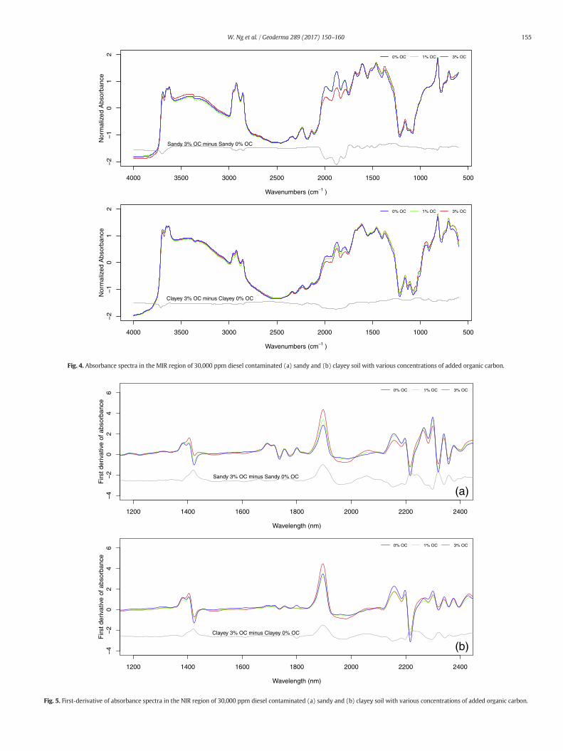
3.1.2. The effect of organic matterRemediation of petroleum-contaminated soil usually involves an ad-

dition of organicmatter to enhance the breakdown of the hydrocarbons.The effect of organic carbon addition is miniscule in the 2990–2810 cm−1 region (the region related to the aliphatic groups/TRH con-centration). However, it affected the region between 2100 and1700 cm−1 (in particular the peaks at 1980, 1870, 1790 cm−1 region,seen in Fig. 4) which is attributed to the quartz overtone. To the bestof our knowledge, the effect of decreasing absorbance in the quartzovertone region due to an increase in organic carbon content has notbeen analysed in other studies. However, this decrease is most likelydue to the formation of mineral and organic carbon complexes in thesoil. This complex has low sorption affinity for hydrocarbons, whichmight cause decrease absorption.

In the NIR region, visually, no specific peak on the absorption spectracan be seen to be affected by the organic matter. Thus, the first deriva-tive of the absorption spectra was used to determine the affected wave-length (seen in Fig. 5), particularly in the 1400, 1900, and 2200–2400 nm region. From the derivative spectra, it can be deduced that ad-dition of organic matter affected the region for hydroxides (1400,

4000 3500 3000 2500 2000 1500 1000 500

−2

−1

01

2

Wavenumbers (cm−1 )

0% OC 1% OC 3% OC

Nor

mal

ized

Abs

orba

nce

Sandy 3% OC minus Sandy 0% OC

4000 3500 3000 2500 2000 1500 1000 500

−2

−1

01

2

Wavenumbers (cm−1 )

0% OC 1% OC 3% OC

Nor

mal

ized

Abs

orba

nce

Clayey 3% OC minus Clayey 0% OC

Fig. 4. Absorbance spectra in the MIR region of 30,000 ppm diesel contaminated (a) sandy and (b) clayey soil with various concentrations of added organic carbon.

1200 1400 1600 1800 2000 2200 2400

−4

−2

02

46

Wavelength (nm)

0% OC 1% OC 3% OC

Firs

t der

ivat

ive

of a

bsor

banc

e

Sandy 3% OC minus Sandy 0% OC

(a)

1200 1400 1600 1800 2000 2200 2400

−4

−2

02

46

Wavelength (nm)

0% OC 1% OC 3% OC

(b)

Firs

t der

ivat

ive

of a

bsor

banc

e

Clayey 3% OC minus Clayey 0% OC

Fig. 5. First-derivative of absorbance spectra in the NIR region of 30,000 ppm diesel contaminated (a) sandy and (b) clayey soil with various concentrations of added organic carbon.

155W. Ng et al. / Geoderma 289 (2017) 150–160

2850 2900 2950

0.0

0.2

0.4

0.6

0.8

1.0

1.2

(a)

Wavenumber

Pro

ject

ed A

bsor

banc

e

2850 2900 2950

0.0

0.2

0.4

0.6

0.8

1.0

1.2

(b)

Wavenumber

Pro

ject

ed A

bsor

banc

e

2850 2900 2950

0.0

0.2

0.4

0.6

0.8

1.0

1.2

(c)

Wavenumber

Pro

ject

ed A

bsor

banc

e

2850 2900 2950

0.0

0.2

0.4

0.6

0.8

1.0

1.2

(d)

Wavenumber

Pro

ject

ed A

bsor

banc

e

2850 2900 2950

0.0

0.2

0.4

0.6

0.8

1.0

1.2

(e)

Wavenumber

Pro

ject

ed A

bsor

banc

e

2850 2900 2950

0.0

0.2

0.4

0.6

0.8

1.0

1.2

(f)

Wavenumber

Pro

ject

ed A

bsor

banc

e

2850 2900 2950

0.0

0.2

0.4

0.6

0.8

1.0

1.2

(g)

Wavenumber

Pro

ject

ed A

bsor

banc

e

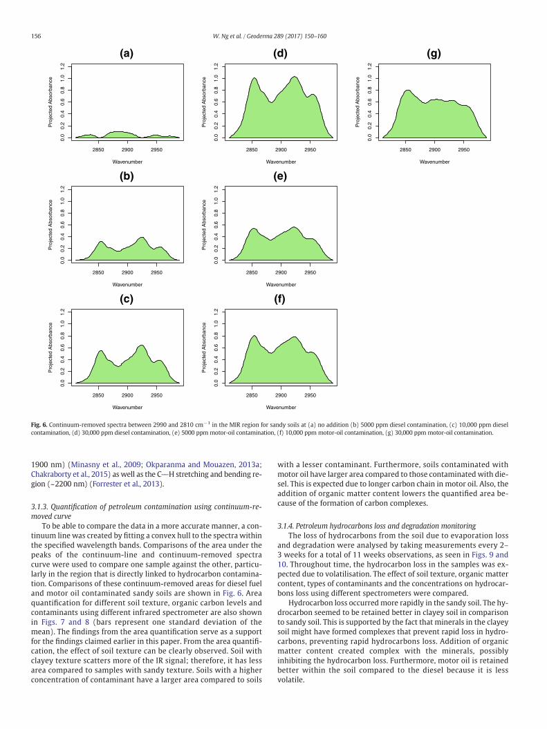
Fig. 6. Continuum-removed spectra between 2990 and 2810 cm−1 in the MIR region for sandy soils at (a) no addition (b) 5000 ppm diesel contamination, (c) 10,000 ppm dieselcontamination, (d) 30,000 ppm diesel contamination, (e) 5000 ppm motor-oil contamination, (f) 10,000 ppm motor-oil contamination, (g) 30,000 ppm motor-oil contamination.

156 W. Ng et al. / Geoderma 289 (2017) 150–160

1900 nm) (Minasny et al., 2009; Okparanma and Mouazen, 2013a;Chakraborty et al., 2015) as well as the C\\H stretching and bending re-gion (~2200 nm) (Forrester et al., 2013).

3.1.3. Quantification of petroleum contamination using continuum-re-moved curve

To be able to compare the data in a more accurate manner, a con-tinuum line was created by fitting a convex hull to the spectra withinthe specified wavelength bands. Comparisons of the area under thepeaks of the continuum-line and continuum-removed spectracurve were used to compare one sample against the other, particu-larly in the region that is directly linked to hydrocarbon contamina-tion. Comparisons of these continuum-removed areas for diesel fueland motor oil contaminated sandy soils are shown in Fig. 6. Areaquantification for different soil texture, organic carbon levels andcontaminants using different infrared spectrometer are also shownin Figs. 7 and 8 (bars represent one standard deviation of themean). The findings from the area quantification serve as a supportfor the findings claimed earlier in this paper. From the area quantifi-cation, the effect of soil texture can be clearly observed. Soil withclayey texture scatters more of the IR signal; therefore, it has lessarea compared to samples with sandy texture. Soils with a higherconcentration of contaminant have a larger area compared to soils

with a lesser contaminant. Furthermore, soils contaminated withmotor oil have larger area compared to those contaminated with die-sel. This is expected due to longer carbon chain in motor oil. Also, theaddition of organic matter content lowers the quantified area be-cause of the formation of carbon complexes.

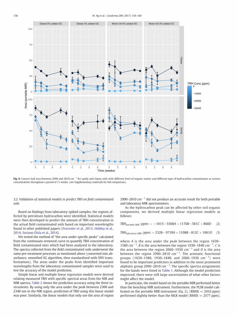
3.1.4. Petroleum hydrocarbons loss and degradation monitoringThe loss of hydrocarbons from the soil due to evaporation loss

and degradation were analysed by taking measurements every 2–3 weeks for a total of 11 weeks observations, as seen in Figs. 9 and10. Throughout time, the hydrocarbon loss in the samples was ex-pected due to volatilisation. The effect of soil texture, organic mattercontent, types of contaminants and the concentrations on hydrocar-bons loss using different spectrometers were compared.

Hydrocarbon loss occurredmore rapidly in the sandy soil. The hy-drocarbon seemed to be retained better in clayey soil in comparisonto sandy soil. This is supported by the fact that minerals in the clayeysoil might have formed complexes that prevent rapid loss in hydro-carbons, preventing rapid hydrocarbons loss. Addition of organicmatter content created complex with the minerals, possiblyinhibiting the hydrocarbon loss. Furthermore, motor oil is retainedbetter within the soil compared to the diesel because it is lessvolatile.

Fig. 7. Convex hull area between 2990 and 2810 cm−1 for sandy and clayey soils with different level of organic matter and different type of hydrocarbon contaminants at variousconcentrations using the portable MIR spectrometer. (Error bars represents ± 1SD).

Fig. 8. Convex hull area between 2300 and 2340 nm for sandy and clayey soils with different level of organic matter and different type of hydrocarbon contaminants at variousconcentrations using portable vis-NIR spectrometers. (Error bars represents ± 1SD).

157W. Ng et al. / Geoderma 289 (2017) 150–160

Diesel 0% added OC Diesel 3% added OC Motor Oil 0% added OC Motor Oil 3% added OC

0

25

50

75

100

0

25

50

75

100

Cla

yey

0 3 6 9 0 3 6 9 0 3 6 9 0 3 6 9

Time (weeks)

Area (

porta

ble

MIR

)

−30000

−20000

−10000

0

TRH Conc.(ppm)

Fig. 9. Convex hull area between 2990 and 2810 cm−1 for sandy and clayey soils with different level of organic matter and different type of hydrocarbon contaminants at variousconcentrations throughout a period of 11 weeks. (see Supplementary materials for full comparison).

158 W. Ng et al. / Geoderma 289 (2017) 150–160

3.2. Validation of statistical models to predict TRH on field contaminatedsoils

Based on findings from laboratory-spiked samples, the regions af-fected by petroleum hydrocarbon were identified. Statistical modelswere then developed to predict the amount of TRH concentration inthe actual field contaminated soils based on important wavelengthsfound in other published papers (Forrester et al., 2013; Hobley et al.,2014; Soriano-Disla et al., 2014).

We tested the method of “the area under specific peaks” calculatedfrom the continuum-removed curve to quantify TRH concentration offield contaminated sites which had been analysed in the laboratory.The spectra collected from the field contaminated soils underwent thesame pre-treatment processes as mentioned above (converted into ab-sorbance, smoothed SG algorithm, then standardized with SNV trans-formations). The areas under the peaks from identified importantwavelengths from the laboratory contaminated samples were used totest the accuracy of the model prediction.

Simple linear and multiple linear regression models were derivedrelating measured TRH with specific spectral areas from the NIR andMIR spectra. Table 2 shows the prediction accuracy using the three in-struments. By using only the area under the peak between 2300 and2340 nm in the NIR region, prediction of TRH using this linear modelwas poor. Similarly, the linear models that only use the area of region

2990–2810 cm−1 did not produce an accurate result for both portableand laboratory MIR spectrometers.

As the hydrocarbon peak can be affected by other soil organiccomponents, we derived multiple linear regression models asfollows:

TRHportable MIR ppmð Þ ¼ −1015−5500Aþ 1176B−581C þ 860D ð2Þ

TRHlaboratory MIR ppmð Þ ¼ 2328−9739Aþ 1108B−812C þ 1061D ð3Þ

where A is the area under the peak between the region 1630–1580 cm−1, B is the area between the region 1930–1840 cm−1, C isthe area between the region 2060–1930 cm−1 and D is the areabetween the region 2990–2810 cm−1. The aromatic functionalgroups (1630–1580, 1930–1840, and 2060–1930 cm−1) werefound to be important predictors in addition to the more prominentaliphatic group 2990–2810 cm−1. The specific spectra assignmentsfor the bands were listed in Table 1. Although the model predictionimproved, there were still large uncertainties of what other factorsmight affect the model.

In particular, the model based on the portableMIR performed betterthan the benchtop MIR instrument. Furthermore, the PLSR model cali-brated on the portable MIR instrument (Eq. 2), (RMSE = 2416 ppm)performed slightly better than the MLR model (RMSE = 2577 ppm).

Diesel 0% added OC Diesel 3% added OC Motor Oil 0% added OC Motor Oil 3% added OC

0

1

2

3

4

5

0

1

2

3

4

5

Cla

yey

Sa

nd

y

0 3 6 9 0 3 6 9 0 3 6 9 0 3 6 9

Time (weeks)

Are

a (

po

rta

ble

NIR

)

−30000

−20000

−10000

0

TRH Conc.(ppm)

Fig. 10. Convex hull area between 2300 and 2340 nm for sandy and clayey soils with different level of organic matter and different type of hydrocarbon contaminants at variousconcentrations throughout a period of 11 weeks. (see Supplementary materials for full comparison).

159W. Ng et al. / Geoderma 289 (2017) 150–160

Importantly, this error is lower than the Health Screening Level (HSL)for direct soil contact in residential areas of 18,500 ppm, and ESL of3400–7540 ppm (NEPC, 2011a).

Table 2Prediction of Total Recoverable Hydrocarbon (TRH) using spectra from different instruments ansion, PLSR is partial least squares regression, R2 is coefficient of determination, RMSE is root me(cal), and leave-one-out cross validation (cv).

Instrument Predictors np R2 cal

Portable NIR LR (2300–2340 nm) 2 0.25Portable NIR PLSR (500–2450 nm)

N components = 9196 0.84

Portable MIR LR 2990–2810 cm−1 2 0.57Portable MIR MLR

1630–1580 cm−1

1930–1840 cm−1

2060–1930 cm−1

2990–2810 cm−1

5 0.75

Portable MIR PLSR (4000–650 cm−1)N components = 8

180 0.89

Laboratory MIR LR2990–2810 cm−1

2 0.38

Laboratory MIR MLR1630–1580 cm−1

1930–1840 cm−1

2060–1930 cm−1

2990–2810 cm−1

5 0.59

Laboratory MIR PLSR (4000–650 cm−1)N components = 9

177 0.89

Here, the models are compared in terms of cross validated R2 andRMSE, and also AIC values. In terms of cross validation, the PLSRmodelsgenerally showed good prediction (Table 2). However, we are also

d different number of predictors (np). LR is linear regression,MLR ismultiple linear regres-an squared error, and AIC is the Akaike Information Criterion calculated on calibration data

RMSE cal (ppm) AIC cal R2 cv RMSE cv (ppm)

4135 1511 0.17 44491881 1786 0.58 3383

3138 1477 0.54 32332393 1438 0.71 2577

1592 1730 0.75 2416

3754 1492 0.34 3862

3037 1457 0.53 3263

1601 1724 0.77 2308

160 W. Ng et al. / Geoderma 289 (2017) 150–160

aware that themodelmaybe overfitting the data (Anderssen et al., 2006).Large numbers of parameters are used to create the PLSR model, com-paredwith only 4 parameters used to create theMLRmodel. The PLSR co-efficients for the portable and laboratory MIR (results presented inSupplementary materials) show different parts of the spectra as impor-tant predictors. More importantly, the PLSR models loadings and coeffi-cients did not consider petroleum hydrocarbon peaks (2990–2810 cm−1) as useful predictors. The PLSR models are able to fit thedata better as they use a higher number of parameters as opposed tothe linear model. It is notable that although the leave-one-out cross vali-dation (cv) has higher RMSE values compared to calibration data (cal),theperformance ranking for both cv and cal are the same (Table 2). Essen-tially cross validation provided the same information as calibration. Crossvalidation is known to provide an over-optimistic estimates ofmodel per-formance and also can cause overfitting (Anderssen et al., 2006; Faber andRajko, 2007; Esbensen and Geladi, 2010).

As an alternative, we evaluated the performance of the models tak-ing into account their complexity or number of parameters. The resultsfor laboratory MIR (Table 2) show that although the PLSR models pro-duce the bestfit in terms of R2 andRMSE values, however the highnum-ber of parameters does not compensate for the improvement in RMSEvalues as calculated by AIC. The multiple linear models which use only4 regions in the MIR consistently have lower AIC values, indicatingthat simpler models are preferred. This theoretical model quantificationof TRH can be improved when more observations are collected.

4. Conclusions

This research exploredmethods for rapid detection of petroleum con-tamination in soils and demonstrated that infrared spectrometry can beutilized. In the laboratory experiment where soil samples were spikedwith different concentrations of petroleum products, it was found thatthe portable mid-infrared spectrometer collected similar spectra as thelaboratory benchtop mid-infrared spectrometer. Therefore, the portableMIR spectrometer could be used as a reliable soil sensor. The importantinfrared regions to quantify hydrocarbon contamination are near 2990–2810 cm−1 (MIR), and 2300–2340 nm (NIR). The clay and carbon con-tents were found to decrease the TRH spectra signal. The laboratory con-taminated soil study showed that throughout the study period of11 weeks, hydrocarbon losses due to volatilisation and degradationwere negligible compared to other factors, such as soil texture, organiccarbon content and types of contaminants.

Based on the laboratory results, attempts were made to predict pe-troleum hydrocarbon concentration on field contaminated soils fromNIR and MIR spectra. It was found that TRH can be predicted with amultiple linearmodel developed using only 4 regions in theMIR spectra(R2portable MIR = 0.71; R2

lab MIR= 0.53). There is an indication that com-monly-used PLSRmodels potentially overfit the data by utilizing a largenumbers of parameters. Therefore, future development ofmodels basedon infrared spectra should consider the fundamental bands as predic-tors. Although more datasets are needed to build a more robustmodel, an initial estimation of petroleum contamination can be obtain-ed from this multiple linear regression model approach. Further workwill look into the predictability of different carbon fractions of the TRH.

Acknowledgements

The authors acknowledge Environmental Earth Sciences for provid-ing the field contaminated samples. This work is part of an ARC LinkageProject LP150100566 - Optimised field delineation of contaminatedsoils.

Appendix A. Supplementary data

Supplementary data to this article can be found online at http://dx.doi.org/10.1016/j.geoderma.2016.11.030.

References

Akaike, H., 1974. A new look at the statistical model identification. IEEE Trans. Autom.Control 19, 716–723.

Anderssen, E., Dyrstad, K., Westad, F., Martens, H., 2006. Reducing over-optimism in var-iable selection by cross-model validation. Chemom. Intell. Lab. Syst. 84 (1–2), 69–74.

Arlot, S., Celisse, A., 2010. A Survey of Cross-validation Procedures for Model Selection.pp. 40–79.

Chakraborty, S., Weindorf, D.C., Li, B., Aldabaa, A.A.A., Ghosh, R.K., Paul, S., Ali, M.N., 2015.Development of a hybrid proximal sensing method for rapid identification of petro-leum contaminated soils. Sci. Total Environ. 514, 399–408.

Clark, R.N., 1999. Spectroscopy of rocks and minerals, and principles of spectroscopy. Re-mote sensing for the earth science. Manual of Remote Sensing, third ed. vol. 3. JohnWiley and Sons, New York.

Clark, R.N., Roush, T.L., 1984. Reflectance spectroscopy: quantitative analysis techniquesfor remote-sensing applications. J. Geophys. Res. 89 (B7), 6329–6340.

CRCCARE (Cooperative Research Centre for Contamination Assessment and Remediationof the Environment), 2015s. Annual Report 2014–2015. Cooperative Research Centrefor Contamination Assessment and Remediation of the Environment, Newcastle, Aus-tralia. (Available at:). http://www.crccare.com/files/dmfile/CRCCARE_AnnualReport_2014-15.pdf.

Esbensen, K.H., Geladi, P., 2010. Principles of proper validation: use and abuse of re-sam-pling for validation. J. Chemom. 24 (3–4), 168–187.

Faber, N.M., Rajko, R., 2007. How to avoid over-fitting in multivariate calibration - the con-ventional validation approach and an alternative. Anal. Chim. Acta 595 (1–2), 98–106.

Forrester, S.T., Janik, L., Mc Laughlin, M., 2010. An Infrared Spectroscopic Test for Total Pe-troleum Hydrocarbon (TPH) Contamination in Soils. Proceedings of the 19th WorldCongress of Soil Science, Soil Solutions for a Changing World, Brisbane, Australia.

Forrester, S.T., Janik, L.J., McLaughlin, M.J., Soriano-Disla, J.M., Stewart, R., Dearman, B.,2013. Total petroleum hydrocarbon concentration prediction in soils using diffuse re-flectance infrared spectroscopy. Soil Sci. Soc. Am. J. 77 (2), 450–460.

Hastie, T., Tibshirani, R., Friedman, J., 2009. The Elements of Statistical Learning. second ed.Springer Series in StatisticsSpringer-Verlag, New York (Data mining, inference, andprediction).

Hobley, E., Willgoose, G.R., Frisia, S., Jacobsen, G., 2014. Vertical distribution of charcoal ina sandy soil: evidence from DRIFT spectra and field emission scanning electron mi-croscopy. Eur. J. Soil Sci. 65 (5), 751–762.

Horta, A., Malone, B., Stockmann, U., Minasny, B., Bishop, T.F.A., McBratney, A.B., Pallasser,R., Pozza, L., 2015. Potential of integrated field spectroscopy and spatial analysis forenhanced assessment of soil contamination: a prospective review. Geoderma 241,180–209.

Minasny, B., McBratney, A.B., Pichon, L., Sun, W., Short, M.G., 2009. Evaluating near infra-red spectroscopy for field prediction of soil properties. Aust. J. Soil Res. 47 (7),664–673.

NEPC (National Environment Protection Council), 2011a. Schedule B1 - Guideline on In-vestigation Levels for Soil and Groundwater. National Environment Protection (As-sessment of Site Contamination) Measure (NEPM), Canberra, Australia (StandingCouncil on Environment and Water. Available at: http://www.scew.gov.au/system/files/resources/93ae0e77-e697-e494-656f-afaaf9fb4277/files/schedule-b1-guideline-investigation-levels-soil-and-groundwater-sep10.pdf).

NEPC (National Environment Protection Council), 2011b. Schedule B3 - Guideline on Lab-oratory Analysis of Potentially. Contaminated Soils, National Environment Protection(Assessment of Site Contamination) Measure (NEPM), Canberra, Australia (StandingCouncil on Environment and Water. Available at: http://www.scew.gov.au/system/files/resources/93ae0e77-e697-e494-656f-afaaf9fb4277/files/schedule-b3-guideline-laboratory-analysis-potentially-contaminated-soils-sep10.pdf).

Okparanma, R.N., Mouazen, A.M., 2013a. Visible and near-infrared spectroscopy analysisof a polycyclic aromatic hydrocarbon in soils. Sci. World J. vol. 2013, 160360 (9pages, 2013).

Okparanma, R.N., Mouazen, A.M., 2013b. Determination of total petroleum hydrocarbon(TPH) and polycyclic aromatic hydrocarbon (PAH) in soils: a review of spectroscopicand nonspectroscopic techniques. Appl. Spectrosc. Rev. 48 (6), 458–486.

R Core Team, 2016. R: A Language and Environment for Statistical Computing. R Founda-tion for Statistical Computing, Vienna, Austria Available at:. https://www.R-project.org/.

Rinnan, A., van den Berg, F., Engelsen, S.B., 2009. Review of the most common pre-pro-cessing techniques for near-infrared spectra. TrAC Trends Anal. Chem. 28 (10),1201–1222.

Sadler, R., Connell, D., 2003. Analytical Methods for the Determination of Total PetroleumHydrocarbons in Soil. Proceedings of the 5th National Workshop on the Assessmentof Site Contamination, May 2003NEPC Serv. Corp., Adelaide, SA, Australia.

Schwartz, G., Ben-Dor, E., Eshel, G., 2012. Quantitative analysis of total petroleum hydro-carbons in soils: comparison between reflectance spectroscopy and solvent extrac-tion by 3 certified laboratories. Appl. Environ. Soil Sci.

Soriano-Disla, J.M., Janik, L.J., Rossel, R.A.V., Macdonald, L.M., McLaughlin, M.J., 2014. Theperformance of visible, near-, and mid-infrared reflectance spectroscopy for predic-tion of soil physical, chemical, and biological properties. Appl. Spectrosc. Rev. 49(2), 139–186.

Viscarra Rossel, R.A., Adamchuk, V.I., Sudduth, K.A., McKenzie, N.J., Lobsey, C., 2011. Prox-imal soil sensing: an effective approach for soil measurements in space and time. Adv.Agron. 113, 237–282.

Viscarra Rossel, R.A., Raphael, A., McBratney, A.B., Minasny, B., 2010. Proximal soil sensing.Progress in soil scienceSpringer, Dordrecht; New York.